HUMAN STRATEGIES IN THE CONTROL OF TIME CRITICAL UNSTABLE SYSTEMS

by

Mircea Florian Lupu

Bachelor of Science in Automation and Computer Engineering,

“Politehnica” University of Timisoara, Romania, 2007

Submitted to the Graduate Faculty of

Swanson School of Engineering in partial fulfillment

of the requirements for the degree of

Master of Science in Electrical Engineering

University of Pittsburgh

201

0

UNIVERSITY OF PITTSBURGH

SWANSON SCHOOL OF ENGINEERING

This thesis was presented

by

Mircea Florian Lupu

It was defended on

November 20, 2009

and approved by

Zhi-Hong Mao, PhD, Assistant Professor, Electrical and Computer Engineering

Patrick Loughlin, PhD, Professor, Bioengineering and Electrical and Computer Engineering

Mingui Sun, PhD, Professor, Neurological Surgery

Thesis Advisor: Zhi-Hong Mao, PhD, Assistant Professor, Electrical and Computer Engineering

ii

Copyright © by Mircea Florian Lupu

2010

iii

HUMAN STRATEGIES IN THE CONTROL OF TIME CRITICAL UNSTABLE SYSTEMS

Mircea Florian Lupu, M.S.

University of Pittsburgh, 2010

The purpose of this study is to investigate the human manual control strategy when balancing an

inverted pendulum under time critical constraints. The strategy was assessed through the

quantification and evaluation of human response while performing tasks that require fast reaction

from the human operator. The results show that as the task becomes more difficult due to

increased time delay or shortened pendulum length, the human operator adopts a more discrete-

type strategy. Additionally, dissimilarities between control of a short pendulum and a delayed

pendulum are identified and discussed. Finally, the discrete-control mechanism is interpreted by

relating the observed human responses to human-performance models. These results can be

applied to systems requiring human interaction, such as teleoperation, which could be designed

to maximize human response.

iv

TABLE OF CONTENTS

ACKNOWLEDGEMENTS ........................................................................................................ X

1.0 INTRODUCTION....................................................................................................... 1

1.1 BACKGROUND ................................................................................................ 1

1.2 MOTIVATION .................................................................................................. 4

2.0 METHODS .................................................................................................................. 5

2.1 INVERTED PENDULUM SYSTEM............................................................... 5

2.2 EXPERIMENT DESCRIPTION...................................................................... 7

3.0 RESULTS .................................................................................................................... 9

3.1 BALANCING THE INVERTED PENDULUM WITH TIME DELAY ...... 9

3.1.1 Movement velocity ...................................................................................... 12

3.1.2 Magnitude of angular sway........................................................................ 13

3.1.3 Frequency of angular sway ........................................................................ 14

3.1.4 Reaction time............................................................................................... 15

3.1.5 Precision of corrective movements ............................................................ 16

3.2 BALANCING A SHORT-LENGTH PENDULUM...................................... 18

3.2.1 Movement velocity ...................................................................................... 19

3.2.2 Magnitude of angular sway........................................................................ 20

3.2.3 Frequency of angular sway ........................................................................ 21

3.2.4 Reaction time............................................................................................... 22

v

3.2.5 Precision of corrective movements ............................................................ 23

4.0 DISCUSSION ............................................................................................................ 26

4.1 DIFFERENT STRATEGIES OF DISCRETE CONTROL......................... 27

4.2 HUMAN PERFORMANCE MODELING.................................................... 28

4.2.1 Human operator as a PD controller with three-state relay and time delay ............................................................................................................ 28

4.2.2 Human operator as an act-and-wait controller........................................ 34

4.3 EVALUATION OF THE EXPERIMENT .................................................... 36

5.0 CONCLUSION ......................................................................................................... 38

APPENDIX.................................................................................................................................. 40

BIBLIOGRAPHY....................................................................................................................... 42

vi

LIST OF TABLES

Table 3-I Standard deviations of the distribution of Γ and γ relative to time delay .................... 18

Table 3-II Standard deviations of the distribution of Γ and γ relative to pendulum length......... 24

Table 4-I Required mental computation for evaluation of movement.......................................... 29

Table 4-II Parameters of the PD controller with three-state relay and time delay resembling the average behavior of the human operator..................................................................... 30

Table A-I Description of the inverted pendulum parameters. ...................................................... 40

vii

LIST OF FIGURES

Figure 2.1 The inverted pendulum system adapted from [18]........................................................ 6

Figure 2.2 The inverted pendulum computer simulation [18]. ....................................................... 8

Figure 3.1 Inverted pendulum control with (a) no delay, (b) 150ms, (c) 300ms, and (d) 500ms time delay.................................................................................................................... 11

Figure 3.2 Movement velocity relative to time delay. .................................................................. 12

Figure 3.3 Magnitude of the angular sway increased with time delay. ........................................ 13

Figure 3.4 Frequency of angular sway relative to time delay....................................................... 15

Figure 3.5 Reaction time of human operator to the angle deviation............................................. 16

Figure 3.6 Reaction time between consecutive movements. ........................................................ 16

Figure 3.7 Distribution of the pendulum angle when movement starts Γ, and when movement ends γ. ......................................................................................................................... 17

Figure 3.8. Inverted pendulum control of a long beam (a), and a short beam (b). ....................... 19

Figure 3.9 Average movement velocity........................................................................................ 20

Figure 3.10 Magnitude of angular sway of the long pendulum and the short pendulum. ............ 21

Figure 3.11 Frequency of angular sway of the long pendulum and the short pendulum.............. 22

Figure 3.12 Reaction time between consecutive movements. ..................................................... 23

Figure 3.13 Distribution of the pendulum angle when movement starts Γ, and when movement ends γ. ...................................................................................................................... 24

Figure 4.1 Inverted pendulum control model from [8]. ................................................................ 29

viii

Figure 4.2 Pendulum angle trajectory of long pendulum control with (a) no delay, (b) 150ms, (c) 300ms, and (d) 500ms time delay, from experiment (left), and simulation (right). ... 33

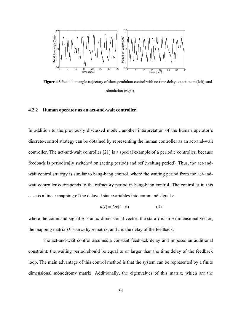
Figure 4.3 Pendulum angle trajectory of short pendulum control with no time delay: experiment (left), and simulation (right)........................................................................................ 34

ix

x

ACKNOWLEDGEMENTS

This thesis could not have been accomplished without the motivation and inspiration provided by

my advisor Dr. Zhi-Hong Mao. I would like to thank him for his full support, and his contagious

optimistic and dynamic view on this extraordinary combined field of control theory and human

interaction. I would also like to thank Professor Luis Chaparro and Professor Alex Jones, who

have had a significant impact on my development as a graduate student and who have made my

experiences as a teaching assistant very enjoyable. I still have a great deal to learn from the

exceptional faculty of the Electrical and Computer Engineering Department of the Swanson

School of Engineering, and I am looking forward to interacting with many other people as my

work continues throughout the coming years.

I would also like to express my humble gratitude to my parents who have supported and

encouraged my every decision, even now from far away. Additionally, I would like to thank my

best friend Ana, whose patience and critical eye have enriched my work, and with whom I will

share all my wonderful and difficult moments from now on.

This effort would not have been as pleasant without my lab colleagues, Robert, Vikram,

Ang, Greg, Seda, Shuang, Hao, Massimo, and Brandon, and without all of my other wonderful

friends who help to make Pittsburgh a great place to call “home”.

1.0 INTRODUCTION

Evaluation of human manual control when performing a difficult task is important for

understanding human movement behavior as well as for identifying human limitations. This

study investigates the manual control of an inverted pendulum, which is an unstable system.

Experimental results have shown that when the control task is difficult and demands a fast

response, such as in the case of a short length pendulum or when time delay affects the task, the

human operator adopts a discrete-type control strategy (i.e. the human response is intermittent

rather than continuous). The objective of this study is to identify and analyze the

continuity/intermittency characteristics of human manual control. Classifying human control

strategies is valuable for characterizing and quantifying human performance, and can aid in the

design of systems that take maximum advantage of the human control movement.

1.1 BACKGROUND

Research into human control started in the late 1940’s with the pioneering work of Tustin [1],

who attempted to improve the servomechanism response of gun turrets by replacing the human

controller with a transfer function. In the next two decades, seminal research was conducted on

the evaluation of human performance, and on the development of correspondent theoretic models

of the human operator [2]-[8]. Birmingham and Taylor [2] used evidence that human operators

1

achieve better results when they perform simple control tasks to suggest solutions for improving

the man-machine control system by reducing the contribution of the human operator to a simple

amplifier. Simpler control tasks imply less complex mental computation by the human operator.

The idea that complex mental computation required by the task directly affects the performance

of the human operator will also be discussed in this study in chapter 4.0 . McRuer [3] followed

the direction of Tustin, focusing on the identification of a more general transfer function

representation of the human operator that would reproduce the advantages of human control. Jex

[4] and Smith [5] evaluated the performance of the human operator when performing tasks at the

limit of stability. The results were then related to the values of the parameters of the transfer

function representation of the human operator, and the boundaries of these values were

graphically displayed and interpreted. Meanwhile, Kleinman [6] concentrated on representing the

human operator as an optimal controller. A historical overview of the progress made in manual

control research is provided by Pew [7], who states that most of the models developed in the

1950’s and 1960’s are still used today, and that no significant innovation has been done since

then. Despite great technological progress in the past decades, which has made possible the

implementation of complex human operator models, there are still important tasks that require

direct human intervention. Characteristics of human control such as adaptation, learning

capabilities, and decision making skills require the human operator to continue to perform certain

manual tasks that are too complicated to be accomplished by machines.

The control of inherently unstable systems such as unstable aircraft, booster rockets, and

the inverted pendulum has attracted significant attention and research efforts [8]-[12] due to its

challenging properties. Young and Meiry [8] discussed manual control of high-order unstable

systems, and noted that human subjects tended to adopt a discrete, or bang-bang strategy in this

2

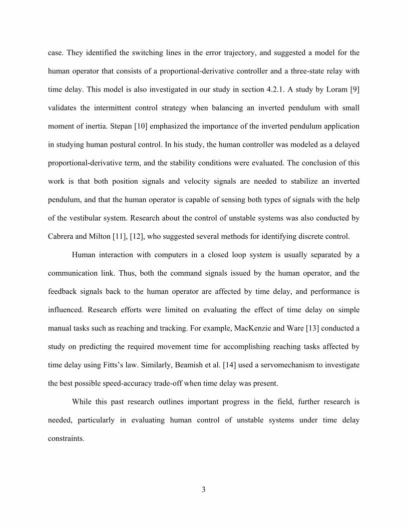
case. They identified the switching lines in the error trajectory, and suggested a model for the

human operator that consists of a proportional-derivative controller and a three-state relay with

time delay. This model is also investigated in our study in section 4.2.1. A study by Loram [9]

validates the intermittent control strategy when balancing an inverted pendulum with small

moment of inertia. Stepan [10] emphasized the importance of the inverted pendulum application

in studying human postural control. In his study, the human controller was modeled as a delayed

proportional-derivative term, and the stability conditions were evaluated. The conclusion of this

work is that both position signals and velocity signals are needed to stabilize an inverted

pendulum, and that the human operator is capable of sensing both types of signals with the help

of the vestibular system. Research about the control of unstable systems was also conducted by

Cabrera and Milton [11], [12], who suggested several methods for identifying discrete control.

Human interaction with computers in a closed loop system is usually separated by a

communication link. Thus, both the command signals issued by the human operator, and the

feedback signals back to the human operator are affected by time delay, and performance is

influenced. Research efforts were limited on evaluating the effect of time delay on simple

manual tasks such as reaching and tracking. For example, MacKenzie and Ware [13] conducted a

study on predicting the required movement time for accomplishing reaching tasks affected by

time delay using Fitts’s law. Similarly, Beamish et al. [14] used a servomechanism to investigate

the best possible speed-accuracy trade-off when time delay was present.

While this past research outlines important progress in the field, further research is

needed, particularly in evaluating human control of unstable systems under time delay

constraints.

3

1.2 MOTIVATION

Teleoperation is an attractive field due to important potential benefits, including handling objects

or performing services in locations that are either hostile or impossible to reach for humans.

Sheridan [15] identifies some of the current applications of manual control in teleoperation. He

recognizes the importance of teleoperation in operating vehicles and systems in outer space. An

example is provided by the remote manipulator system (RMS) which is controlled by a human

operator with the help of two three-axis joysticks in order to move heavy loads outside a space

shuttle. By 1980, remote operated vehicles (ROV) were widely used for underwater operations.

Such robots play an important role in the offshore oil and gas industry, including inspection of

underwater welds, monitoring pipelines, or placing anodes. Marine biologists rely on remote

vehicles for investigating the undersea fauna. Teleorobotics is also used in military operations to

provide extended vision for soldiers in highly dangerous locations, navigate over mine fields,

and observe enemy operations.

An important emerging field centered on human manual control is telesurgery [16], [17].

The use of teleoperation in surgical procedures has many promising benefits because it allows

physicians to provide medical expertise without traveling to the location of the patient.

Additionally, the surgeon can rely on telerobotics to reach places not accessible by the human

hands. Our investigation in this study can be of importance in the field of telesurgery, where the

human operator performs a task that requires high precision over a network channel which

induces significant amount of time delay.

Some of the above mentioned systems are unstable [8]-[12], which poses a greater

challenge for the human operator. Our study is focused on balancing an inverted pendulum,

which is an inherently unstable system.

4

2.0 METHODS

An experiment was conducted to evaluate the strategies of the human operators when controlling

an unstable system such as the inverted pendulum. In this chapter the dynamics of the inverted

pendulum are introduced, and the experiment setup is described.

2.1 INVERTED PENDULUM SYSTEM

The human-controlled inverted pendulum system [18] considered in the study is shown in Figure

2.1. The dynamics of the inverted pendulum are described by the following differential equation

2 2 2

2 2cos sin3 2 2

mL d mL d x mgLdt dtθ θ θ+ = (1)

where is the mass of the pendulum, is the length of the pendulum, m L θ is the angle of the

pendulum relative to the vertical position, x is the displacement of the bottom tip of the

pendulum, and is the gravitational acceleration (please refer to the g Appendix for a complete

derivation of the equation).

5

Figure 2.1 The inverted pendulum system adapted from [18].

By approximating the nonlinear terms in (1) such that cos 1θ ≈ , and sinθ θ≈ for small values

of the angle θ , the inverted pendulum transfer function is simplified to the form

( ) ( )

2 2

2

1( )( )( ) 1 1

s ss g gH s

X s Ts Tss

α

α

− −Θ

= = =+ −−

(2)

where 3 2g Lα = , s is the Laplace variable, and 1 2T α= = 3L g is the time constant of the

inverted pendulum system which varies with the length of the pendulum L.

The above obtained linear time-invariant system has as input the displacement x , and as

output the angle of the pendulum relative to the vertical position θ . The poles of the transfer

function are α±=2,1s . Hence, the system is unstable due to the real positive pole. In order to

simulate the inverted pendulum dynamics on the computer, the discrete transfer function with a

sample time of Ts = 50 ms was obtained from (2), and written in state space form

1 0[ 1] [ ] [

1

[ ] 0 [ ] [ ]

s

s

T]

s

x k x kT T

y k x k u kg g

α

α α

⎧ ⎡ ⎤ ⎡ ⎤+ = +⎪ ⎢ ⎥ ⎢ ⎥

⎪ ⎣ ⎦ ⎣ ⎦⎨

⎡ ⎤⎪ = − −⎢ ⎥⎪ ⎣ ⎦⎩

u k (3)

where [ ] [ ][ ] ,Tx k kθ θ⎡ ⎤= ⎦⎣& k .

6

2.2 EXPERIMENT DESCRIPTION

In order to observe the human control strategies when balancing an inverted pendulum, an

experiment with seven subjects was conducted. A planar inverted-pendulum system was

considered in this study [Figure 2.1]. Instead of physical implementation of the inverted

pendulum, a real-time simulation in Matlab/Simulink was used following the idea of Bodson

[18] [Figure 2.2]. The subjects balanced the inverted pendulum using a Logitech ATK3 joystick

connected to a computer whose screen provided visual feedback to the subjects. Artificial delays

were introduced in the simulation to emulate transport delays in teleoperation.

The subjects were asked to try their best to maintain a long pendulum of 20 m in the

upright position under zero delay and under a delay of 150, 300, and 500 ms. The subjects were

also asked to balance a short pendulum of 5 m without time delay. Note that the pendulum length

considered for the computer simulation should not be regarded as corresponding to the

pendulum-balancing task in the real environment because in the experiment the human operator

did not experience the force feedback from the inverted pendulum. Moreover, in the computer

simulation the movement of the joystick corresponded to the bottom tip displacement of the

pendulum which was proportional to the pendulum length. However, using the simulated

pendulum system, the difficulty of the stabilization task was still closely related to the length of

the pendulum. When the pendulum was long enough and under zero time delay, the human

operator experienced no difficulty in control, but when the pendulum was sufficiently short (i.e.

5 m), the human operator was challenged.

For each considered scenario, five successful trials were recorded in which the pendulum

was balanced without falling. Each trial was 45 seconds long, and the trials were tested in a

random order with a 15 second break between successive trials.

7

Figure 2.2 The inverted pendulum computer simulation [18].

The quantitative measures of the human performance that were considered in our study

are the following:

• Velocity of hand movement

• Magnitude of the pendulum’s angular sway

• Frequency of the pendulum’s angular sway (i.e. number of times the pendulum crossed

the upright position in one second)

• Reaction time of the human operator to the angle deviation of the pendulum

• Pendulum angle when the correction movement started, and when the correction

movement stopped.

8

3.0 RESULTS

It was observed that, as the balancing task became more difficult, the subjects adjusted their

strategy in order to keep the pendulum in the stable upright position. When balancing the long-

length pendulum without time delay, the subjects experienced no difficulties, and they exhibited

a more continuous type of control. However, as the time delay increased, the human operators

exhibited more apparent discrete-type, or bang-bang-like actions in their control. A similar type

of control was identified when balancing the short-length pendulum.

3.1 BALANCING THE INVERTED PENDULUM WITH TIME DELAY

The trajectory of the pendulum angle, the time derivative of the pendulum angle, and the velocity

of the movement of a representative subject (Subject 4) are shown in Figure 3.1 for comparison

between manual control strategies with different time delays. Although a recorded trial was 45

seconds long, the figures do not include the first 10 seconds of the trial, when the subjects tended

to make use of the initial upright position of the pendulum. The subjects waited during this time

period for the pendulum to start falling to one side before triggering any corrective movement. In

order to perceive the change of strategy of the human operator as the time delay increased, the

case when no time delay affected the task [Figure 3.1 (a)] is shown first. The human operator

strategy in this case yields characteristics of more continuous control. An important

9

characteristic of this type of control is that movements are not time critical (i.e. the pendulum

system has a large time constant), which allows the human operator enough time to initiate the

balancing movement, and then to make corresponding corrections if needed. This behavior can

be noticed in Figure 3.1 (a) in the velocity profile of the movement between 18 and 23 seconds

or between 27 and 31 seconds, where the subject executes 3 - 4 consecutive tiny movements in

the same direction to correct the displacement of the pendulum form the upright position. The

small magnitudes of the angle velocity and the movement velocity reveal that a smoother hand

movement trajectory was exhibited when no time delay was present, compared to the behavior

affected by time delay.

As the amount of time delay increased, the performance of the human operator was

affected, and a change in the control strategy could be recognized. Figure 3.1 (b)-(d) show the

adopted human operator control approach when time delay was 150 ms, 300 ms, and 500 ms,

respectively. As the time delay was increased, spike-form profiles of the movement velocity

became more apparent. This indicates that the human operator tended to make more sudden

moves. The magnitude of these peaks increased with time delay, such that when the time delay

was 500 ms, one corrective movement was enough to cause the pendulum to pass the stable

upright position to the opposite side.

The average trend of the movement velocity, angular sway, angular sway rate and the

reaction time of the human operator will be investigated in the next sections.

10

0 5 10 15 20 25 30 35-50

0

50

Time (Sec)

Ang

le (D

eg)

0 5 10 15 20 25 30 35-10

-5

0

5

10

Time (Sec)

Ang

le V

eloc

ity (D

eg/S

ec)

0 5 10 15 20 25 30 35-4

-2

0

2

4

Time (Sec)Car

t Vel

ocity

(Met

er/S

ec)

0 5 10 15 20 25 30 35-50

0

50

Time (Sec)

Ang

le (D

eg)

0 5 10 15 20 25 30 35-10

-5

0

5

10

Time (Sec)

Ang

le V

eloc

ity (D

eg/S

ec)

0 5 10 15 20 25 30 35-4

-2

0

2

4

Time (Sec)C

art V

eloc

ity (M

eter

/Sec

)

(a) (b)

0 5 10 15 20 25 30 35-50

0

50

Time (Sec)

Ang

le (D

eg)

0 5 10 15 20 25 30 35

-10

-5

0

5

10

Time (Sec)

Ang

le V

eloc

ity (D

eg/S

ec)

0 5 10 15 20 25 30 35-4

-2

0

2

4

Time (Sec)

Car

t Vel

ocity

(Met

er/S

ec)

0 5 10 15 20 25 30 35-50

0

50

Time (Sec)

Ang

le (D

eg)

0 5 10 15 20 25 30 35-10

-5

0

5

10

Time (Sec)

Ang

le V

eloc

ity (D

eg/S

ec)

0 5 10 15 20 25 30 35-4

-2

0

2

4

Time (Sec)

Car

t Vel

ocity

(Met

er/S

ec)

(c) (d)

Figure 3.1 Inverted pendulum control with (a) no delay, (b) 150ms, (c) 300ms, and (d) 500ms time delay.

11

3.1.1 Movement velocity

The hand movement velocity exhibited by all the seven subjects and the average movement

velocity are shown in Figure 3.2. Most subjects followed a similar trend, with movements

becoming faster with increasing time delay. Thus, the human operator tried to compensate for the

effect of delay by making faster and more sudden hand movements. Subject 2 slowed down the

control movements when the time delay was 150 ms, and Subjects 3, 5 and 7 slowed down their

movement when the time delay was 300 ms. However, Subject 1 did not seem to follow the

average tendency and can be identified as an exception for which we will try to find an

explanation later in the study.

0 100 200 300 400 5000

0.05

0.1

0.15

0.2

0.25

0.3

0.35

0.4

Delay (ms)

Car

t vel

ocity

(m/s

)

Subject 1Subject 2Subject 3Subject 4Subject 5Subject 6Subject 7Average

Figure 3.2 Movement velocity relative to time delay.

12

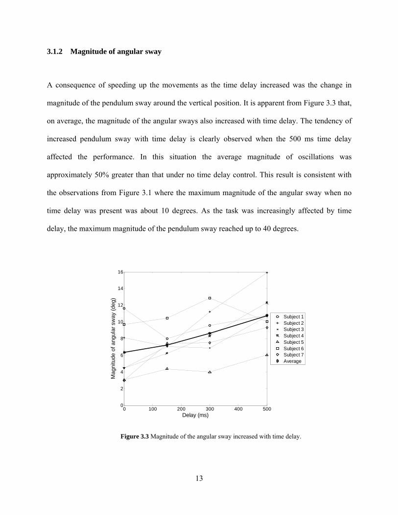
3.1.2 Magnitude of angular sway

A consequence of speeding up the movements as the time delay increased was the change in

magnitude of the pendulum sway around the vertical position. It is apparent from Figure 3.3 that,

on average, the magnitude of the angular sways also increased with time delay. The tendency of

increased pendulum sway with time delay is clearly observed when the 500 ms time delay

affected the performance. In this situation the average magnitude of oscillations was

approximately 50% greater than that under no time delay control. This result is consistent with

the observations from Figure 3.1 where the maximum magnitude of the angular sway when no

time delay was present was about 10 degrees. As the task was increasingly affected by time

delay, the maximum magnitude of the pendulum sway reached up to 40 degrees.

0 100 200 300 400 5000

2

4

6

8

10

12

14

16

Delay (ms)

Mag

nitu

de o

f ang

ular

sw

ay (d

eg)

Subject 1Subject 2Subject 3Subject 4Subject 5Subject 6Subject 7Average

Figure 3.3 Magnitude of the angular sway increased with time delay.

13

Individually, each subject exhibited in general an increased magnitude of pendulum sway

as the time delay increased. The performance of Subject 4 is consistent with the average

tendency of the magnitude of the pendulum sway as time delay increased. Subjects 1 and 2 have

a slight decrease in the pendulum sway at 150 ms time delay, and Subjects 3, 5 and 7

experienced the same tendency at 300 ms. The magnitude of the pendulum sway of Subject 6

increased when time delay was 150 ms and 300 ms, but when time delay was 500 ms, it was

comparable to the case when no time delay affected the task. It is important to note how these

results are in concordance with the individual performances of the subjects presented in the

previous section.

3.1.3 Frequency of angular sway

Both the magnitude of the angular sway and the frequency of oscillations of the pendulum

around the upright position are affected by the amount of time delay. Figure 3.4 shows the

frequency of the angular sway over the different time delays of all the subjects averaged over all

trials. For Subjects 1 and 5 a decrease in the frequency of the angular sway with each time delay

was obvious, but Subjects 2, 3, 4 and 7 exhibited only a general trend of decrease in the

frequency of oscillation. However, Subject 6 proved once again to be an exception to the average

trend, as the frequency of the angular sway increased slightly with time delay. The average

frequency of oscillation, which is shown with the bold line in Figure 3.4, changed inversely with

the amount of time delay. This result is expected as we observed that the magnitude of angular

sway increased with time delay. Thus, the observed manual strategy of balancing an inverted

pendulum under time delay resembled less frequent movements of larger magnitude as the delay

increased.

14

0 100 200 300 400 5000

0.1

0.2

0.3

0.4

0.5

0.6

0.7

0.8

0.9

Delay (ms)

Freq

uenc

y of

ang

ular

sw

ay (H

z)

Subject 1Subject 2Subject 3Subject 4Subject 5Subject 6Subject 7Average

Figure 3.4 Frequency of angular sway relative to time delay.

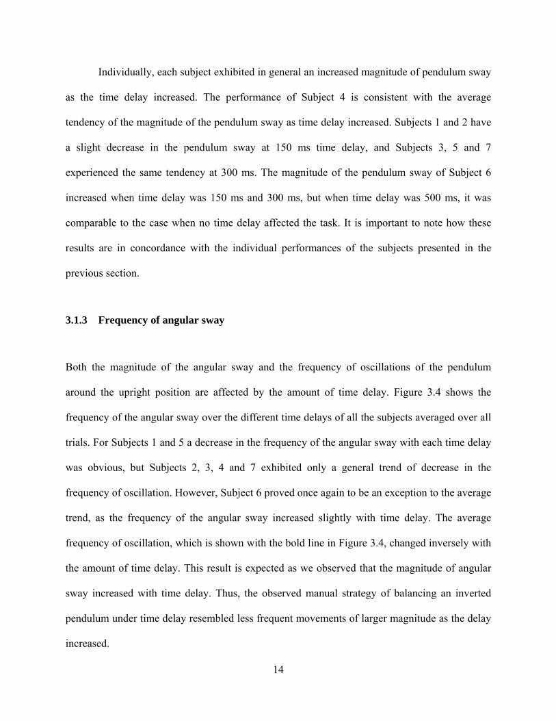
3.1.4 Reaction time

The human operator reaction time is defined in this study as the time interval between two

consecutive corrective movements (Figure 3.5). Figure 3.6 presents the average reaction time

over all trials and over all subjects as the subjects experienced different time delays. The average

reaction time was observed to decrease when time delay was 150 ms, but seemed to follow an

increasing trend as time delay increased to 300 ms and 500 ms. The large value for the reaction

time when no time delay was present is caused by the performance of the Subjects 1 and 6 which

can be considered exceptions. The increasing trend of the reaction time with the amount of time

delay supports the argument that movements become less frequent as time delay increases.

15

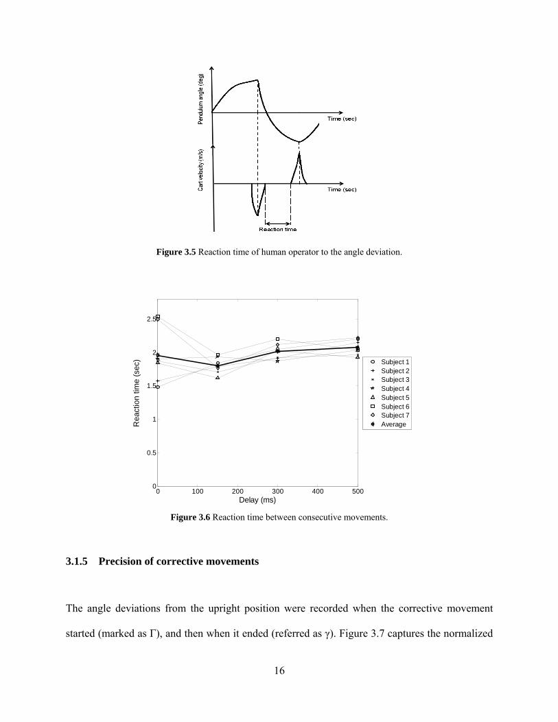
Figure 3.5 Reaction time of human operator to the angle deviation.

0 100 200 300 400 5000

0.5

1

1.5

2

2.5

Delay (ms)

Rea

ctio

n tim

e (s

ec)

Subject 1Subject 2Subject 3Subject 4Subject 5Subject 6Subject 7Average

Figure 3.6 Reaction time between consecutive movements.

3.1.5 Precision of corrective movements

The angle deviations from the upright position were recorded when the corrective movement

started (marked as Γ), and then when it ended (referred as γ). Figure 3.7 captures the normalized

16

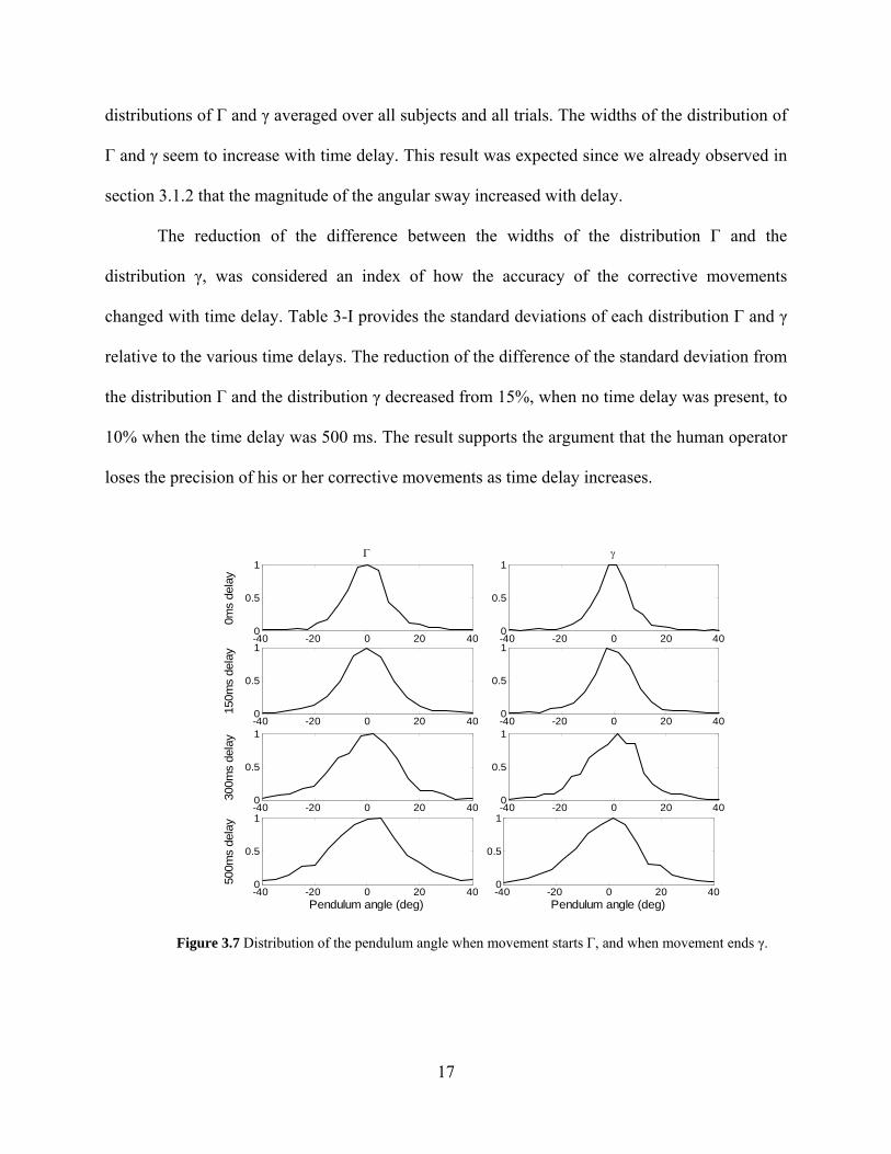
distributions of Γ and γ averaged over all subjects and all trials. The widths of the distribution of

Γ and γ seem to increase with time delay. This result was expected since we already observed in

section 3.1.2 that the magnitude of the angular sway increased with delay.

The reduction of the difference between the widths of the distribution Γ and the

distribution γ, was considered an index of how the accuracy of the corrective movements

changed with time delay. Table 3-I provides the standard deviations of each distribution Γ and γ

relative to the various time delays. The reduction of the difference of the standard deviation from

the distribution Γ and the distribution γ decreased from 15%, when no time delay was present, to

10% when the time delay was 500 ms. The result supports the argument that the human operator

loses the precision of his or her corrective movements as time delay increases.

-40 -20 0 20 400

0.5

1

0ms

dela

y

Γ

-40 -20 0 20 400

0.5

1γ

-40 -20 0 20 400

0.5

1

150m

s de

lay

-40 -20 0 20 400

0.5

1

-40 -20 0 20 400

0.5

1

300m

s de

lay

-40 -20 0 20 400

0.5

1

-40 -20 0 20 400

0.5

1

500m

s de

lay

Pendulum angle (deg)-40 -20 0 20 400

0.5

1

Pendulum angle (deg)

Figure 3.7 Distribution of the pendulum angle when movement starts Γ, and when movement ends γ.

17

Table 3-I Standard deviations of the distribution of Γ and γ relative to time delay

0 ms delay 150 ms delay 300 ms delay 500 ms delay

Stv( )Γ 0.21 0.22 0.24 0.31

Stv( )γ 0.17 0.18 0.21 0.25

Stv( )-Stv( ) *100Stv( )

γΓΓ

15.02% 14.48% 13.84% 10.55%

3.2 BALANCING A SHORT-LENGTH PENDULUM

We also conducted an experiment to observe the human strategy when a short pendulum

was balanced for the purpose of comparing the results with those of the time delay control. A

simulated pendulum of length 5 m was determined empirically to be short enough to challenge

the human operator. Similarities and differences between the two strategies will be examined.

The trajectory profile of the pendulum angle, velocity of the pendulum angle, and

velocity of the movement of a representative subject (the same as in Figure 3.1) are illustrated in

Figure 3.8. It is apparent that the profile of the movement velocity exhibits a very similar spike-

form pattern (a characteristic of discrete control) as the one in Figure 3.1 (d). The magnitude of

these spikes is much smaller than that of the spikes which represent controlling the pendulum

under time delay [refer to Figure 3.1 (b)-(d)], but comparable with the magnitude of the

movement velocity when a long pendulum without time delay was balanced. Due to the short

length of the pendulum, each of the peaks observed in the movement velocity profile

corresponded to a sway of the pendulum on the other side relative to the upright position.

Therefore, the frequency of the angular sway is expected to be higher for the shorter pendulum

18

than for the long pendulum. Moreover, the frequency of the spikes in the velocity profile seemed

greater when a short pendulum was balanced. Thus, when balancing a short pendulum, the

human operator appeared to make sudden movements similar to those made when balancing a

delayed pendulum, but the movements were quicker and of smaller magnitude. This result will

be investigated for validation in the next sections.

0 5 10 15 20 25 30 35-50

0

50

Time (Sec)

Ang

le (D

eg)

0 5 10 15 20 25 30 35-10

-5

0

5

10

Time (Sec)

Ang

le V

eloc

ity (D

eg/S

ec)

0 5 10 15 20 25 30 35

-0.5

0

0.5

Time (Sec)

Car

t Vel

ocity

(Met

er/S

ec)

0 5 10 15 20 25 30 35-50

0

50

Time (Sec)

Ang

le (D

eg)

0 5 10 15 20 25 30 35-10

-5

0

5

10

Time (Sec)

Ang

le V

eloc

ity (D

eg/S

ec)

0 5 10 15 20 25 30 35

-0.5

0

0.5

Time (Sec)

Car

t Vel

ocity

(Met

er/S

ec)

(a) (b)

Figure 3.8. Inverted pendulum control of a long beam (a), and a short beam (b).

3.2.1 Movement velocity

The average movement velocity is shown in Figure 3.9, which indicates that the average

movement velocity when balancing a short pendulum is similar to the hand movement velocity

when balancing a pendulum without time delay. Subjects 1 and 6 are again exceptions. The fact

that the average movement velocity when balancing a long pendulum without time delay is close

19

to the average movement velocity when balancing a short pendulum seems counterintuitive.

However, we have to recall that, because the human subjects made use of a joystick to control

the pendulum and the pendulum lengths differ in the two situations, the former case resembles a

similar spike-form velocity profile, but the spikes are not alternating as in the latter case.

To be noticed that the average hand movement velocity of all subjects was measured to

be 0.1 m/s when controlling a short pendulum, which was less than any average movement

velocity measured under time delay [refer to Figure 3.2].

Figure 3.9 Average movement velocity.

3.2.2 Magnitude of angular sway

The averaged absolute value of the magnitude of angular sway over all subjects when controlling

a short pendulum is illustrated in Figure 3.10. Disregarding the results of Subjects 1 and 6, the

magnitude of the angular sway of all other subjects was larger when controlling a short

pendulum than when controlling a long pendulum. Averaged over all subjects, this tendency was

clear as the magnitude of the short pendulum sway was 9 deg, and the magnitude of the long

20

pendulum sway was 6 deg. This result was expected since in the previous section we noticed that

the magnitude of the movement velocity when balancing a short pendulum was similar to the

magnitude of the movement velocity when balancing a long pendulum. When applying similar

force to balance pendulums of different lengths, it makes sense that the short pendulum would

expose larger magnitude sway.

When comparing these results with those obtained when controlling the delayed

pendulum, we can observe that the magnitude of sway of the short pendulum was smaller than

that of the pendulum under 500 ms delay (11 deg), but similar to that of the pendulum under 300

ms time delay (approximately 9 deg).

Figure 3.10 Magnitude of angular sway of the long pendulum and the short pendulum.

3.2.3 Frequency of angular sway

The average frequency of crossing the upright position is shown in Figure 3.11 for all subjects.

By omitting the performance of Subjects 1 and 6, it is evident that the frequency of the angular

sway was higher when controlling a short pendulum (0.8 Hz) than when controlling a long

pendulum (0.6 Hz). This result is predictable, as the frequency of occurrence of the “peaks” in

21

the movement velocity profile of the short pendulum was higher than that of the peaks from the

movement velocity of the long pendulum.

The frequency of the angular sway when controlling a short pendulum (0.8 Hz) was

visibly higher than the frequency of the angular sway when time delay was involved (from

Figure 3.4: 150 ms time delay – 0.6 Hz, 300 ms time delay – 0.55 Hz, 500 ms time delay – 0.5

Hz). This observation confirms the idea that different types of discrete control can be

distinguished.

Figure 3.11 Frequency of angular sway of the long pendulum and the short pendulum.

3.2.4 Reaction time

The reaction time of all subjects when controlling a short pendulum and a long pendulum are

illustrated in Figure 3.12. The reaction time was noticeably smaller when controlling a short

pendulum than when controlling a long pendulum. The averaged reaction time of all subjects

was 1.2 seconds when controlling a short pendulum, and 1.9 seconds when controlling a long

pendulum. As we have already observed, the reaction time increased as time delay affected the

performance. Hence, the human operator was making quicker movements when controlling a

22

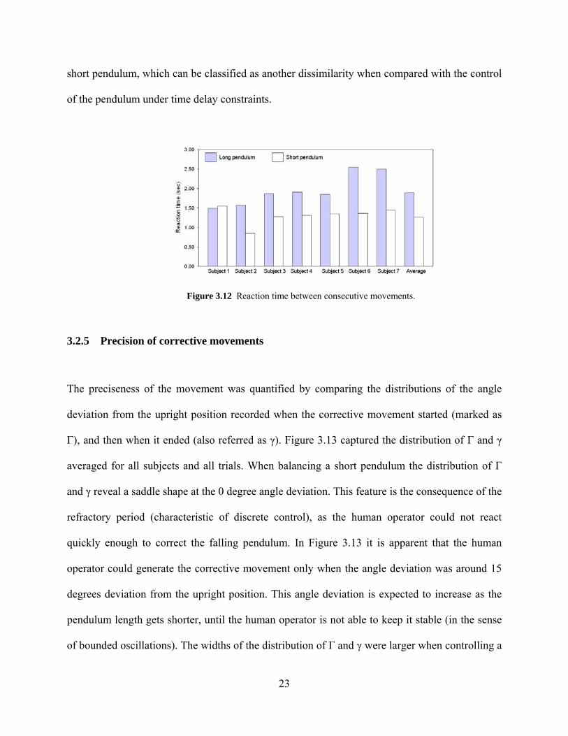
short pendulum, which can be classified as another dissimilarity when compared with the control

of the pendulum under time delay constraints.

Figure 3.12 Reaction time between consecutive movements.

3.2.5 Precision of corrective movements

The preciseness of the movement was quantified by comparing the distributions of the angle

deviation from the upright position recorded when the corrective movement started (marked as

Γ), and then when it ended (also referred as γ). Figure 3.13 captured the distribution of Γ and γ

averaged for all subjects and all trials. When balancing a short pendulum the distribution of Γ

and γ reveal a saddle shape at the 0 degree angle deviation. This feature is the consequence of the

refractory period (characteristic of discrete control), as the human operator could not react

quickly enough to correct the falling pendulum. In Figure 3.13 it is apparent that the human

operator could generate the corrective movement only when the angle deviation was around 15

degrees deviation from the upright position. This angle deviation is expected to increase as the

pendulum length gets shorter, until the human operator is not able to keep it stable (in the sense

of bounded oscillations). The widths of the distribution of Γ and γ were larger when controlling a

23

short pendulum as compared to both the control of a long pendulum without time delay, and the

control of the pendulum under any time delay.

-40 -20 0 20 400

0.2

0.4

0.6

0.8

1Lo

ng p

endu

lum

Γ

-40 -20 0 20 400

0.2

0.4

0.6

0.8

1γ

-40 -20 0 20 400

0.2

0.4

0.6

0.8

1

Sho

rt pe

ndul

um

Pendulum angle (deg)-40 -20 0 20 400

0.2

0.4

0.6

0.8

1

Pendulum angle (deg)

Figure 3.13 Distribution of the pendulum angle when movement starts Γ, and when movement ends γ.

Table 3-II Standard deviations of the distribution of Γ and γ relative to pendulum length.

Long pendulum Short pendulum

Stv( )Γ 0.21 0.31

Stv( )γ 0.17 0.23

Stv( )-Stv( ) *100Stv( )

γΓΓ

15.02% 26.79%

The reduction of the difference between the widths of the distribution Γ and the

distribution γ, is shown in Table 3-II. Particularly, the reduction of the difference of the standard

deviation between the distribution Γ and γ increased from 15%, as in the case of the long

24

pendulum, to 26.8% as in the case of the short pendulum. From these results, it appears that the

human operator achieves more precise movements when controlling a short pendulum, which is

partially true. However, it is important to keep in mind that the standard deviation of Γ was

larger when controlling the short pendulum (0.31) than in all the other cases (no delay – 0.21;

150 ms delay – 0.22; 300 ms delay – 0.24; 500 ms delay – 0.28). Also, the standard deviation of

γ (0.23) was comparable with the cases when time delay was 300 ms (0.21) and 500 ms (0.25).

Thus, the corrective movements of the human operator when balancing a short pendulum,

although generated at a larger angle deviation, are similar to the corrective movements generated

when time delay affected the movement.

25

4.0 DISCUSSION

The experimental results show that, when the task of balancing an inverted pendulum becomes

more difficult, human control becomes more discrete. The human operators did not experience

major difficulties when balancing a sufficiently long pendulum with no delay. The long

pendulum with large a time constant allowed the human subjects enough time to prepare the

movement before actually performing it. However, when the task became more difficult due to

increased time delay or shortened pendulum length, the subjects adopted a discrete, or bang-

bang, type of control. This has a certain “open-loop” nature for each stroke or pulse of

movement, because the feedback information cannot be evaluated in time in order to generate the

best possible performance. Discrete or bang-bang control is known to appear in minimum-time

tasks and to exhibit an abrupt change between two states [19]. Another relevant characteristic of

discrete control is the occurrence of a refractory period between switching states [11], [12].

In the rest of this section we will compare the discrete-type strategies between the control

of the pendulum with time delay and the control of a short pendulum. We will also consider

different human-performance models to suggest possible explanations for the discrete control of

the human operator. Finally, we will evaluate the conducted experiment.

26

4.1 DIFFERENT STRATEGIES OF DISCRETE CONTROL

The pendulum-angle and movement-velocity profiles in Figure 3.1 (d) (subject to a time delay of

500 ms) exhibit strong similarities with the corresponding profiles in Figure 3.8 (b), where the

human operator controlled a short pendulum. In both cases, the pendulum swayed in a range of

±40 deg, and the maximum amplitude of the angle velocity was about 5 deg/s. However, there

are dissimilarities between the two cases in certain aspects of discrete control.

First, the average movement velocity in balancing the short pendulum was smaller than

those observed in control of the long pendulum with time delays, but close to the average

movement velocity seen when balancing the long pendulum without time delay. Second, the

frequency with which the pendulum crossed the upright position (with or without time delay)

was smaller than the frequency observed when balancing the short pendulum without delay.

Moreover, the average reaction time when controlling a short pendulum is smaller than the

reaction time when controlling any of the long pendulums, and is approximately half the average

reaction time when controlling the long pendulum with the maximum considered time delay.

The above differences are characteristics that can help to distinguish between different

types of discrete control. When balancing the long pendulum with time delay, the task is difficult

because it demands the ability of the human operator to make predictions in order to compensate

for the delayed perception of system responses. Here the adopted strategy for discrete control is

to create sudden faster but less frequent movements. On the other hand, when the balancing task

is difficult due to the shortened length of the pendulum (with reduced time constant), faster

reactions of lesser intensity are required to stabilize the pendulum. In this case, the movements

are discrete in such a way that more frequent switching is exhibited. Note that Loram [9] reached

the same results on the inverted pendulum balancing task when the moment of inertia was very

27

small (i.e. the moment of inertia is directly proportional with the square of the length of the

pendulum).

4.2 HUMAN PERFORMANCE MODELING

In human manual control, the neural system needs time to plan and execute a movement. This

process is constrained not only by the latency in sensory feedback and muscle activation but also

by the mental computation required for generating the desired command signal for the muscles.

When the task becomes difficult due to the fast dynamics of the system under control (the short

pendulum) or to the demanded capability of motion prediction (control under time delay), mental

computation is challenged and the discrete-control strategy can be considered a solution to

resolve these challenges.

4.2.1 Human operator as a PD controller with three-state relay and time delay

Young and Meiry [8] revealed a direct relationship between the characteristics of discrete control

and the required mental computation. They suggested that when the generation of human force

involves evaluation of displacements or velocities, the human controller has to mentally compute

at least one integration operation [refer to Table 4-I]. The complex integration operation is time

consuming. When performing an easy balancing task, the human controller has sufficient time to

perform the mental computation and to prepare relatively accurate continuous movements.

However, when the system dynamics require fast action, the human controller does not have

enough time to perform the complex computation for integration and to implement a smooth

28

continuous-type control. Rather, the human controller can adopt a discrete-type control to reduce

the complexity of the mental computation. A pulse-like force pattern makes the mental-

integration process much easier to implement, because the area of the exerted force requires only

the computation of the duration of the action, assuming that the magnitude of the pulses is

constant [Table 4-I]. These are the characteristics exhibited by the discrete control as can be seen

in Figure 3.1 and Figure 3.8.

Table 4-I Required mental computation for evaluation of movement.

Controller Force ΔVelocity Required Mental Computation

Continuous

Full Integration

0

( )t

V F dτ τΔ = ∫

Discrete

Count pulses

ONV r tΔ = ⋅∑

Adapted from [8]

Figure 4.1 Inverted pendulum control model from [8].

Young and Meiry [8] further proposed a human-performance model for manual control as

shown in Figure 4.1. The model consists of a proportional-derivative (PD) controller, a three-

state relay, and a delay component.

29

In order to gain insight into how the human operators may internally adjust their strategy

according to the task difficulty, we implemented the above model in Simulink/Matlab. The

inverted pendulum system used in the simulation was the same discrete state space model

representation that was used for the experiments with the human subjects. For the simulation, the

discrete corresponding components of Figure 4.1 were implemented with the same sample time

of 50 ms seconds as in the experiments.

Table 4-II Parameters of the PD controller with three-state relay and time delay resembling the average

behavior of the human operator.

Pendulum length 20 m 5 m

Time delay τ 0 ms 150 ms 300 ms 500 ms 0 ms a 0.12 0.35 0.53 0.7 0.7 K 9 23 22 18 47 TL 0.2 0.5 0.8 1.35 0.35

The parameters of the PD controller were adjusted such that the response of the system

yielded similar behavior to the average human movement strategy observed in the experiments.

The average response of the human operator is characterized by the frequency within which the

pendulum crosses the vertical upright position, and by the pendulum’s magnitude sway for each

scenario. Table 4-II shows the values of all parameters of the considered human operator model.

To illustrate intuitive parameter tuning we refer to the following procedure: the value a of the

three-state relay (an angle deviation of more than a radians generated a pulse of magnitude K,

and an angle deviation of less than –a radians generated a pulse of magnitude –K) was set for

each scenario to the corresponding angle deviation when the human generated a corrective

movement; afterward, the values of K and TL were generated exhaustively to yield the average

30

human performance regarding the frequency and the magnitude of the angular sway of the

pendulum for each scenario. The value of a is given in radians, as the entire simulation uses this

unit of measure for the pendulum angle.

Figure 4.2 and Figure 4.3 illustrate a comparison between the trajectories of the

pendulum angle from the experiments (on the same subject as in Figure 3.1) and from

simulations using the proposed model for the human operator. A careful inspection of the values

for the human operator model showed in Table 4-II reveals a certain tendency. When balancing a

delayed pendulum, the parameter TL that produced the desired behavior of the proposed human

operator model increased with time delay, while the value of K decreased as time delay

increased. When controlling a short pendulum, the value for TL was smaller than in the cases

where a delayed pendulum was balanced, and was comparable with TL of the long pendulum

without time delay. The value K for the same case was much larger than all the rest. It is

important to note that the parameters of the PD controller are consistent with the stability

conditions of the delayed inverted pendulum system presented by Stepan [10].

The three-state relay switches its output –K/0/K relative to the magnitude of the input a,

which can be regarded as the weighted sum of the angle deviation and the velocity of the angle

deviation from the upright position. To achieve similar performance with the human operator,

the coefficient of the angle velocity TL appeared to increase with the time delay. When the time

delay was 500 ms, the value of derivative gain TL exceeded the unity weight coefficient of the

pendulum angle. This result demonstrates that as time delay affected the task, the human

operator had a tendency to rely increasingly on the changing rate of the error signal (i.e. angle

velocity of the pendulum) to generate the control signal (i.e. the corrective balancing movement).

This prediction capability is consistent with the intuitive idea that the human operator tends to

31

use predictive behavior in order to compensate for latency. Neurological studies identified the

cerebellum to serve as a motion predictor in movement control [20].

The parameter K of the output of the three-state relay generates pulses corresponding to

the amplitude of the force applied on the pendulum (as mentioned in Table 4-II). As the input to

the inverted pendulum system was the displacement of the bottom tip of the pendulum (2), the

force pattern had to be integrated twice. The integration operation is linear and, therefore, the

magnitude of the force is directly related to the magnitude of the displacement of the pendulum’s

bottom tip. Because the parameter a is limiting the magnitude of the angular sway, the parameter

K directly correlates with the frequency of oscillations of the pendulum around the upright

position. To resemble the human operator performance, the value of the parameter K was noted

to decrease with time delay. This result is consistent with the observation that the frequency of

the angular sway decreases with time delay.

When controlling the short pendulum, the parameters of the human operator model

reinforce the idea that the task is difficult due to the need to make quick movements in order to

keep the pendulum balanced. The strategy exhibited by the subjects is consistent with the

tendency observed in the parameter values of the human operator model. The derivative gain TL

is comparable with the case where a long pendulum was balanced without time delay, invoking

limited prediction capabilities in performing the task. Moreover, the parameter K is larger than in

any other scenario, which is in concordance with the high frequency of the angular sway

observed in the experiments from chapter 3.2.

32

0 5 10 15 20 25 30 35

-10

-5

0

5

10

Time (Sec)

Pen

dulu

m a

ngle

(Deg

)

0 5 10 15 20 25 30 35

-10

-5

0

5

10

Time (Sec)

Pen

dulu

m A

ngle

(Deg

)

(a)

0 5 10 15 20 25 30 35-30

-20

-10

0

10

20

30

Time (Sec)

Pen

dulu

m a

ngle

(Deg

)

0 5 10 15 20 25 30 35-30

-20

-10

0

10

20

30

Time (Sec)

Pen

dulu

m A

ngle

(Deg

)

(b)

0 5 10 15 20 25 30 35-50

0

50

Time (Sec)

Pen

dulu

m a

ngle

(Deg

)

0 5 10 15 20 25 30 35-50

0

50

Time (Sec)

Pen

dulu

m A

ngle

(Deg

)

(c)

0 5 10 15 20 25 30 35-50

0

50

Time (Sec)

Pen

dulu

m a

ngle

(Deg

)

0 5 10 15 20 25 30 35-50

0

50

Time (Sec)

Pen

dulu

m A

ngle

(Deg

)

(d)

Figure 4.2 Pendulum angle trajectory of long pendulum control with (a) no delay, (b) 150ms, (c) 300ms,

and (d) 500ms time delay, from experiment (left), and simulation (right).

33

0 5 10 15 20 25 30 35-50

0

50

Time (Sec)

Pen

dulu

m a

ngle

(Deg

)

0 5 10 15 20 25 30 35-50

0

50

Time (Sec)

Pen

dulu

m a

ngle

(Deg

)

Figure 4.3 Pendulum angle trajectory of short pendulum control with no time delay: experiment (left), and

simulation (right).

4.2.2 Human operator as an act-and-wait controller

In addition to the previously discussed model, another interpretation of the human operator’s

discrete-control strategy can be obtained by representing the human controller as an act-and-wait

controller. The act-and-wait controller [21] is a special example of a periodic controller, because

feedback is periodically switched on (acting period) and off (waiting period). Thus, the act-and-

wait control strategy is similar to bang-bang control, where the waiting period from the act-and-

wait controller corresponds to the refractory period in bang-bang control. The controller in this

case is a linear mapping of the delayed state variables into command signals:

( ) ( )u t Dx t τ= − (3)

where the command signal u is an m dimensional vector, the state x is an n dimensional vector,

the mapping matrix D is an m by n matrix, and τ is the delay of the feedback.

The act-and-wait control assumes a constant feedback delay and imposes an additional

constraint: the waiting period should be equal to or larger than the time delay of the feedback

loop. The main advantage of this control method is that the system can be represented by a finite

dimensional monodromy matrix. Additionally, the eigenvalues of this matrix, which are the

34

poles of the closed-loop system, depend on the values of the control matrix D. Thus, the

elements of the matrix D are chosen such that the response of the system is not only stable, but

also allows the system to deliver a good performance. Adaptive or optimal control theory

methods may be used to determine such a control matrix. As in the previous model, the human

operators are assumed to possess capabilities to adjust some internal gains in order to adapt their

movement given the constraints of time delay and small time constant of the controlled system.

Moreover, the act-and-wait controller not only simplifies pole placement of the closed-loop

system but can also stabilize systems that cannot be stabilized by autonomous controllers [21].

This suggests that the act-and-wait control method may be superior compared to other control

methods, and may provide an explanation for why the human operator adopts a discrete-type

control strategy when the task is constrained by time delay.

Beyond the proposed human operator models, many other models have been suggested in

the literature [1]-[5], [10], [21]. They all have in common the idea that adjustments of some

parameters have to be performed in order for the task to be controlled. An adaptive adjustment

process of such parameters to yield the desired human performance could also give insight into

the mechanism involved in obtaining the parameters. Applying control dependent noise in the

considered strategy of the human controller would explain variation in human performance on

each trial.

35

4.3 EVALUATION OF THE EXPERIMENT

The average behavior and the individual performances of the subjects in the conducted

experiment provide evidence that human subjects adopt specific strategies in manual control.

However, certain aspects may have interfered with the obtained results. The subjects did not

know ahead of time how difficult the task would be, as the length of the pendulum and the time

delay of each scenario were not apparent to them. Therefore, they had to use their intuition to

estimate these features after the first few balancing movements. Additionally, the requirement

was to successfully balance the pendulum for 45 seconds, and no trial was recorded when the

pendulum fell in this time period. Each subject had some failed trials, which relates to the

individual capacity of learning the task. As the subjects started to become familiar with the task,

the balancing movements sometimes appeared to become slower not only when the time delay

increased, but also when the pendulum length was shorter. This is due to the capacity of humans

to adapt to the task and continuously improve their performance. This aspect was not accounted

for in our experiment, as we would have liked to evaluate human manual performance at its

limits. The embodiment of such properties in the design of a human controller has been the

aspiration of many researchers in the past decades, and is still an important current research field,

and we may regard this direction for future investigation.

As previously mentioned, two of the seven subjects (Subjects 1 and 6) have proven to be

exceptions in comparison to the other subjects. On one hand, Subject 1 displayed unusually fast

movements, the highest frequency of angular sway, and the smallest reaction time when the

pendulum was long and no time delay was included. On the other hand Subject 6 illustrated the

lowest frequency of angular sway, and the largest reaction time. Additionally, the two largest

sway magnitudes of the pendulum were recorded from these two subjects. These results show

36

that Subject 1 exhibited characteristics of the behavior expected when balancing a short

pendulum. A possible interpretation for this behavior could be the subject’s inability to discern

between a long pendulum and a short pendulum. Subject 6 was observed to have a slow reaction

to the angle deviation of the pendulum. The movements were triggered late such that large

angular sway and large reaction times were recorded. Moreover, Subject 6 had the most

difficulties with the task, as double the time was needed to accomplish the experiment.

37

5.0 CONCLUSION

The analysis of the experiment performed in this study shows that human operators tend to adopt

a discrete control strategy when the task is difficult due to time delay, or small time constant.

When the task of balancing the inverted pendulum became difficult due to time delay constraints,

the discrete-type control method was observed, and subjects exhibited less frequent switching

but with higher speed. This is slightly different from the task of controlling a shorter pendulum

with no delay, where the human operator switched more frequently.

A simple nonlinear model for the human controller was implemented in order to interpret

the discrete-control mechanism. The proposed manual model (consisting of a PD controller, a

delay component, and a three-state relay) resembled general characteristics of discrete-type

control of human operators. The parameters of the PD controller for each scenario were adjusted

such that the response of the system yielded a similar response to that observed in the conducted

experiments. This gave insight into how the human operator adopts the control strategy relative

to the challenging index of the task and the required performance. The derivative gain TL was

increased as time delay increased, implying on one hand that the human operators relied on the

rate of change of the pendulum angle when shaping their corrective balancing movement, and on

the other hand that the pendulum angle had an attenuating role in determining the movement.

This observation confirms the hypothesis that human operators tend to adjust their predictive

gains in order to compensate for latency. Another possible explanation for the human strategy of

38

discrete control can be obtained via a model of act-and-wait control. This theory assumes that the

human operator is capable of adjusting the elements of the matrix that maps the state variables

into command signals in order to stabilize an unstable system.

The results of our study not only reflect the human performance when dealing with

challenging manual control tasks, but also provide a source for investigation of new control

theoretic models that can improve or even reproduce human performance. This exploration is of

great relevance in the field of teleoperation, where human performance plays a key role.

Further research is required to quantify the information content of the human hand

movements in order to provide a qualitative measurement of human performance, and to identify

the limits of manual control. Moreover, the investigation of the information rate achieved by the

human operator has to be made relative to the amount of time delay and the length of the

pendulum.

39

APPENDIX

INVERTED PENDULUM DYNAMICS

The inverted pendulum dynamics are derived with the Lagrangian method. The inverted

pendulum is shown in Figure A.1, and the description of the parameters are given in Table A-I.

Table A-I Description of the inverted pendulum parameters.

Parameter Description

(x0, y0) Coordinates of the bottom tip of the pendulum

(x1, y1) Coordinates of the center of gravity of the pendulum

θ Angle of the pendulum

L Length of the pendulum

m Mass of the pendulum

J Moment of inertia of the pendulum Figure A.1 Inverted pendulum system

The Lagrangian is defined as

.

gL T V= − (A1)

where T is the translational and rotational kinetic energy, and V is the potential energy. Both

quantities are defined at the center of gravity (x1,y1) of the pendulum. The derivation yields

40

( )2 2 21 1

2 22

0

2 22

0

22 2 2

0 0

1 12 2

1 1sin cos2 2 2 2

1 1cos sin2 2 2 2

1 1 1cos2 2 4 2 2

T m x y J

d L d Lm xdt dt

L Lm x J

L Lmx m mx J

θ

Jθ θ θ

θ θ θ θ θ

θ θ θ θ

= + +

⎧ ⎫⎡ ⎤ ⎡ ⎤⎪ ⎪⎛ ⎞ ⎛ ⎞= + +⎨ ⎬⎜ ⎟ ⎜ ⎟⎢ ⎥ ⎢ ⎥⎝ ⎠ ⎝ ⎠⎣ ⎦ ⎣ ⎦⎪ ⎪⎩ ⎭⎧ ⎫⎪ ⎪⎡ ⎤ ⎡ ⎤= + + +⎨ ⎬⎢ ⎥ ⎢ ⎥⎣ ⎦ ⎣ ⎦⎪ ⎪⎩ ⎭

= + + +

&& &

&

& & &&

& & && &

+

(A2)

cos2LV mg θ= (A3)

Due to readability purposes, the notation x dx dt=& was used for the first time derivative of x, and

22x d x dt=&& for the second time derivative of x. Thus, the Lagrangian becomes

22 2 2

0 01 1 1cos cos2 2 4 2 2 2g

L L LL mx m mx J mgθ θ θ θ= + + + −& & && & θ (A4)

The equation that describe the dynamics of the inverted pendulum system were obtained by

computing the Euler-Lagrange equation

0gLL ddtθ θ

∂⎛ ⎞∂− ⎜ ⎟∂ ∂⎝ ⎠&

= (A5)

Which yields 0 sin sin2 2

gL L Lmx mgθ θ θθ

∂= − +

∂&& (A6)

2

0 cos4 2

gL L Lm mx Jθ θθ

∂= + +

∂& &

&θ& (A7)

2

0 0cos sin4 2 2

gLd L L Lm mx mxdt

Jθ θ θ θθ

∂⎛ ⎞= + − +⎜ ⎟∂⎝ ⎠

&& & &&&& &&

θ (A8)

Substituting (A6) and (A8) into (A5)

2 2 2

2 2( ) cos si4 2 2L d mL d x mgLJ m

dt dtθ nθ θ+ + = (A9)

After substituting the moment of inertia 2 12J mL= into (A9), and rearranging the terms, the

relation (1) from section 2.1 is obtained.

41

BIBLIOGRAPHY

[1] A. Tustin, “The nature of the human operator’s response in manual control and its implication for controller design”, Journal of the Institution of Electrical Engineers, vol. 94, pp. 190–201, 1947.

[2] H. P. Birmingham and F. V. Taylor, “A design philosophy for man-machine control systems”, Proceedings of the I.R.E., vol. 42, pp. 1748–1758, December 1954.

[3] D. T. McRuer and E. S. Krendel, “Dynamic response of human operators”, Wright Air Development Center (WADC) TR-56-523 OH, Air Material Command, USAF, 1957.

[4] H. R. Jex, J. D. McDonnell, and A. V. Phatak, “A ‘critical’ tracking task for manual control research”, IEEE Transactions on Human Factors in Electronics, vol. HFE-7, no. 4, pp. 138–145, Dec. 1966.

[5] R. L. Smith, “On the limits of manual control”, IEEE Transactions on Human Factors in Electronics, vol. HFE-4, no. 1, pp. 56–59, 1963.

[6] S. Baron and D. L. Kleinman, “The human as an optimal controller and information processor”, IEEE Transactions on Man-Machine Systems, vol. MMS-10, pp. 9–17, 1969.

[7] R. W. Pew, “More than 50 years of history and accomplishment in human performance model development”, Human Factors, vol. 50, no. 3, pp. 489–496, June 2008.

[8] L. R. Young and J. L. Meiry, “Bang-bang aspects of manual control in high-order systems”, IEEE Transactions on Automatic Control, vol. 10, no. 3, pp. 336–341, July 1965.

[9] I. D. Loram, P. J. Gawthrop, and M. Lakie, “The frequency of human, manual adjustments in balancing an inverted pendulum is constrained by intrinsic physiological factors” Journal of Physiology, vol. 577, pp. 417–432, Nov. 2006.

[10] G. Stepan and L. Kollar, “Balancing with reflex delay”, Mathematical and Computer Modelling, vol. 31, no. 4-5, pp. 199–205, 2000.

[11] J. L. Cabrera and J. G. Milton, “On-off intermittency in a human balancing task”, Physical Review Letters, vol. 89, no. 15, pp. 158 702–1–158 702–4, Oct. 2002.

42

43

[12] J. L. Cabrera, C. Luciani, and J. Milton, “Neural control on multiple time scales: insights from human stick balancing”, Condensed Matter Physics, vol. 9, no. 2, pp. 373–383, 2006.

[13] I. S. MacKenzie and C. Ware, “Lag as a determinant of human performance in interactive systems”, Proceedings of the INTERACT 1993 and CHI 1993 Conference on Human Factors in Computing Systems, pp. 448–493, 1993.

[14] D. Beamish, S. Bhatti, J. Wu, and Z. Jiang, “Performance limitations from delay in human and mechanical motor control”, Biological Cybernetics, vol. 99, no. 1, pp. 43–61, July 2008.

[15] T. B. Sheridan, “Telerobotics”, Automatica, vol. 25, no. 4, pp. 487–507, July 1989.

[16] R. Rayman et al., “Long-distance robotic telesurgery: a feasibility study for care in remote environments”, International Journal of Medical Robotics and Computer Assisted Surgery, vol. 2, pp. 216–224, 2006.

[17] J. M. Thompson, M. P. Ottensmeyer and T. B. Sheridan, “Human factors in tele-inspection and tele-surgery: cooperative manipulation under asynchronous video and control feedback”, Proceedings of the First International Conference on Medical Image Computing and Computer-Assisted Intervention, pp. 368–376, 1998.

[18] M. Bodson, “Fun control experiments with matlab and a joystick”, in Proc. IEEE Conf. Decision and Control, vol. 3, Maui, HI, USA, Dec. 2003, pp. 2508–2513.

[19] F. L. Lewis and V. L. Syrmos, “Optimal Control” (2nd Edition). New York, USA: John Wiley & Sons, Inc., 1995.

[20] R. C. Miall, D. J. Weir, D. M. Wolpert, and J. F. Stein, “Is the cerebellum a smith predictor?”, Journal of Motor Behavior, vol. 25, no. 3, pp. 203–216, Sept. 1993.

[21] T. Insperger, “Act-and-wait concept for continuous-time control systems with feedback delay”, IEEE Transactions on Control Systems Technology, vol. 14, no. 5, pp. 974–977, Sept. 2006.