Department of Construction Sciences

Solid Mechanics

ISRN LUTFD2/TFHF-16/5211-SE(1-51)

Cylinder Volume Deviation

for Heavy Duty Combustion Engines

Master’s Dissertation by

Ivan Anagrius West

Supervisors:

Ola Stenlåås, Scania

Ralf Denzer, Div. of Solid Mech. LTH

Examiner:

Matti Ristinmaa, Div. of Solid Mech. LTH

Copyright © 2016 by the Division of Solid Mechanics

and Ivan Anagrius West

Printed by Media-Tryck AB, Lund, Sweden

For information, address:

Division of Solid Mechanics, Lund University, Box 118, SE-221 00 Lund, Sweden

Webpage: www.solid.lth.se

I

Abstract The automotive industry is a field of enormous competition. Customers and regulations demand

economical and sustainable products. To achieve maximum efficiency, engine systems require

detailed control. To increase the accuracy of the models that describe the combustion process, a

demand has arisen at Scania for an exact prediction of the combustion chamber volume.

During engine operation, the components surrounding the combustion chamber are exposed

thermal forces, pressure forces and mass forces from the reciprocating components. Due to these

forces, the components will deform and the volume of the combustion chamber will deviate from its

ideal volume.

During this master thesis, simulations have been carried out to calculate the mechanical

deformations and approximate the combustion chamber volume deviation. The impact from

production variations on the combustion chamber volume have been investigated. Based on the

results from the simulations, a model has been implemented that approximates the combustion

chamber volume based on linearized relations.

The finished model gives reasonable results that are well in accordance with the time consuming

simulations. The production variations have a relatively large impact on the combustion chamber

volume and define the tolerances of the model.

II

Acknowledgements This master thesis has been done at Scania CV AB in Södertälje, Sweden. I am thankful for all the time

and resources the people at Scania have committed to help me succeed.

First of all, I want to thank my supervisor at Scania, Ola Stenlåås. Without him, this thesis would not

have been possible. Fredrik Haslestad and Ola Jönsson have also been providing me with crucial

support and valuable comments throughout the process.

I would also like to thank Carlos Jorques Moreno, Soheil Salehpour and David Norman for their

important feedback and help. And I want to thank my desk neighbours and master thesis colleagues

Amanda El Rayes and Michail Korres and all of NESC for making my stay here at Scania enjoyable.

And finally I want to thank my supervisor at LTH, Ralf Denzer who has been following my progress

and provided me with valuable feedback.

III

Abbreviations

BDC Bottom Dead Center – Position of the piston when it is nearest to the crankshaft.

CAD Crank Angle Degree – Unit equal to one degree, to measure the piston position and orientation of the crankshaft. CAD is locally defined as zero at TDCC.

CFD Computational Fluid Dynamics

DOF Degree Of Freedom

FE Finite Element

FEM Finite Element Method

LL Lower Limit – The lower limit of an assembly tolerance.

MBS Multibody Simulation

RPM Revolutions Per Minute – Rotational speed of the crankshaft.

RSS Root Sum Square

TDC Top Dead Center - Position of the piston when it is farthest away from the crankshaft.

TDCC Top Dead Center Combustion – TDC between the compression stroke and the power stroke.

TDCGE Top Dead Center Gas Exchange – TDC between the Exhaust stroke and the intake stroke.

UL Upper Limit – The upper limit of an assembly tolerance.

IV

Contents Abstract .................................................................................................................................................... I

Acknowledgements ................................................................................................................................. II

Abbreviations ......................................................................................................................................... III

1 Introduction ..................................................................................................................................... 1

1.1 Background .............................................................................................................................. 1

1.2 Problem formulation ............................................................................................................... 1

1.3 Method .................................................................................................................................... 2

1.4 Delimitations ........................................................................................................................... 2

1.5 Related work ........................................................................................................................... 3

1.6 Outline ..................................................................................................................................... 4

2 Production variations ...................................................................................................................... 5

2.1 Measurements included in stack-up analysis .......................................................................... 7

2.2 Treatment of radial clearances................................................................................................ 8

2.3 Results of the tolerance stack-up analysis .............................................................................. 8

3 Theory of simulations .................................................................................................................... 10

3.1 Dynamic reduction ................................................................................................................ 10

3.2 Connecting rod and piston .................................................................................................... 12

3.3 Couplings of components ...................................................................................................... 12

4 Simulations and post-processing ................................................................................................... 13

4.1 Static deformations ............................................................................................................... 13

4.1.1 Finite Element-model .................................................................................................... 13

4.1.2 Boundary conditions and loads ..................................................................................... 14

4.1.3 Finite element analysis .................................................................................................. 14

4.1.4 Post-processing results .................................................................................................. 14

4.1.5 Volume calculation ........................................................................................................ 15

4.1.6 The ideal piston path ..................................................................................................... 17

4.1.7 The compensated piston path ....................................................................................... 18

4.2 Dynamic deformations .......................................................................................................... 19

4.2.1 External loads on model ................................................................................................ 19

4.2.2 Post-processing the results from the displacement of the connecting rod .................. 19

4.2.3 Post-processing the results of the displacements of the cylinder head ....................... 20

5 Results of simulations .................................................................................................................... 22

5.1 Volume difference due to cold liner distortion ..................................................................... 22

V

5.2 Volume difference due to hot distortion .............................................................................. 23

5.3 Volume increase due to displacement of piston ................................................................... 24

5.4 Volume increase due to deformation of cylinder head ........................................................ 25

6 Model ............................................................................................................................................ 26

6.1 Modelling displacement of the crank-slider mechanism due to mass forces and cylinder

pressure ............................................................................................................................................. 26

6.1.1 Relating deformations to the calculated forces ............................................................ 27

6.1.2 Position of the piston in z-direction .............................................................................. 33

6.2 Modelling the displacements of the crank-slider mechanism due to thermal forces .......... 34

6.3 Deformation of cylinder head due to pressure ..................................................................... 34

6.4 Deformation of cylinder head due to thermal forces ........................................................... 35

6.5 Deformation of cylinder liner due to thermal load ............................................................... 35

6.6 Mechanical tolerances .......................................................................................................... 36

6.7 The final model ...................................................................................................................... 36

7 Results and discussion ................................................................................................................... 37

7.1 Error analysis ......................................................................................................................... 39

7.2 Future work ........................................................................................................................... 40

8 Conclusions .................................................................................................................................... 42

9 Bibliography ................................................................................................................................... 43

1

1 Introduction

1.1 Background The automotive industry is a field of enormous competition. Customers and regulations demand

economical and sustainable products. To achieve maximum efficiency, engine systems require

detailed control. With faster and cheaper computational power and increasing knowledge of the

combustion process, there is potential to improve todays models and achieve an even higher

accuracy in the engine control.

In order to control the engines performance accurately, the combustion process is quantified. This is

today done by a combination of real and virtual sensors, measuring quantities such as pressure,

temperature and mass flow. Due to the difficulty of taking measurements inside the cylinder in a

reliable and non-intrusive way, some events of the combustion are approximated with

thermodynamic models. In the thermodynamic models a number of assumptions are today applied.

One of these assumptions concerns the in-cylinder volume. The in-cylinder volume is calculated as

the volume of a perfect geometrical cylinder plus the volume of the piston bowl. This assumption

neglects production variations and deformation of the cylinder and the slider-crank mechanism. The

question of whether this assumption has a significant impact is the foundation of this master thesis.

1.2 Problem formulation The quantification of the combustion process is central in engine control. It is usually done by

approximation with thermodynamic models. In most of these models a heat release analysis is an

essential part. The most common way of expressing the heat release is in the following equation:

𝜕𝑄

𝜕𝜃=

𝛾

𝛾 − 1𝑝

𝜕𝑉

𝜕𝜃+

1

𝛾 − 1𝑉

𝜕𝑝

𝜕𝜃+

𝜕𝑄𝐻𝑇

𝜕𝜃+

𝜕𝑄𝐶𝑟𝑒𝑣𝑖𝑐𝑒

𝜕𝜃 (1.1)

Where 𝜃 is the crank angle, 𝛾 is the specific heat ratio, 𝑝 is the cylinder pressure, 𝑉 is the cylinder

volume, 𝑄 is the heat released from the combustion, 𝑄𝐻𝑇 is the heat transfer losses and 𝑄𝐶𝑟𝑒𝑣𝑖𝑐𝑒 is

the energy losses due to flow out of the cylinder. [1]

When applying the heat release analysis, one common assumption is to idealize the cylinder volume,

𝑉 in Eq. (1.1), and calculate it as the volume of a perfect geometrical cylinder plus the volume of the

piston bowl. The height of the cylinder is calculated from the position of the piston which in turn is a

function only of the crank angle. This assumption will be referred to as the Idealized cylinder volume

assumption throughout this report.

This Master Thesis aims to develop a model of the true cylinder volume as a function of crank angle,

engine load and engine speed. And to investigate how the true cylinder volume deviates from the

ideal cylinder volume.

To calculate the true cylinder volume, three main sources of deviations will be taken into account.

Production variations.

Static distortion of the cylinder liner.

Dynamic deformation of the cylinder and crank mechanism.

The results of this Master Thesis will bring light on the significance of the idealized cylinder volume

assumption. This knowledge will primarily be of use when applying a heat release analysis. However,

it is not precluded that the result will be of use for other applications within engine control.

2

1.3 Method The overall methodology for this Master Thesis will have a deductive, quantitative, approach. The

solution process will be analytical and theoretical.

The problem in this thesis have an interdisciplinary character, several different contributing factors

have to be considered. Therefor the process to obtain results will include gathering data from

research that has been done and combining it with results from simulations carried out during this

Thesis. The theoretical depth will be emphasised on the latter part.

The volume deviation from the ideal cylinder volume will in this Master Thesis be broken down into

three main parts: Production variations, static deformation of the cylinder liner and dynamic

deformation of the cylinder and crank mechanism.

Production variations. The strategy of investigating the manufacturing variance will involve

reviewing technical drawings and carrying out a tolerance analysis. The approach of the

tolerance analysis that will be applied is the worst-case and the root-sum-square tolerance

accumulation models that are covered in a wide range of literature.

Static deformation of the cylinder liner. Static forces, including residual tension from the

bolts in the cylinder block and thermal forces during operation, will cause the cylinder liner

to deform (usually referred to as cold and hot liner distortion). As this area already has been

subjected to substantial research, I will in this Master Thesis make use of existing results.

Dynamic deformation of the cylinder and crank mechanism. Dynamic forces from the

combustion cycle, including in-cylinder pressure and reciprocating masses, will cause the

cylinder and crank mechanism to deform. The methods to analyse this part will include

Finite Element Analysis, Finite Element dynamic reduction and multibody simulation.

At the point where all results from the three main parts are acquired a post-processing procedure

will be developed to combine the results to a final model. Supporting theory for this part will be

found in literature handling solid mechanics, material behaviour and structural mechanics.

The final model will be based on simulations that are previously validated through experiments,

however no experiments will be carried out during the course of this Master Thesis.

The method of obtaining result will follow this basic path:

1. Problem description

2. Data collection and literature study

3. Definition of goals and delimitations

4. Obtain substantive theory

5. Gather result data and carry out simulations

6. Combine results and describe finalized model

1.4 Delimitations The following delimitations will be applied over the course of this Master Thesis:

The crank angle will be defined locally for each cylinder. The torsion of the crankshaft will not

be considered.

The pressure trace is considered known and synchronized with the crank angle.

The cylinder pressure will be considered uniform.

3

The engine for analysis is a Scania 13 litre in-line 6-cylinder diesel engine without EGR.

However, the process of obtaining results will be clearly outlined to facilitate future analysing

of other engines.

Only specific steady-state operating points will be analysed.

o For static analysis:

1800 RPM and high reference load

o For dynamic analysis:

800 RPM and high reference load

1200 RPM and low reference load

1200 RPM and medium reference load

1200 RPM and high reference load

1600 RPM and high reference load

1900 RPM and high reference load

Effects of blow-by will not be considered.

Effects of wear will not be considered.

1.5 Related work The impact of mechanical deformation on the in-cylinder volume trace has been investigated at Lund

University, however this investigation concerned an optical engine of Bowditch Design [2], [3]. The

result of this study showed that the impact was significant for the heat-release calculation. One

conclusion of this article was that the distorted volume-trace also is of importance for all-metal

engines, but it was not investigated by the authors.

A previous master thesis project at Scania has investigated the torsion of the crankshaft and

developed a model to calculate the true crank angle [4]. The thesis is closely related to this master

thesis as the crank angle for each cylinder is essential in the calculation of the true cylinder volume.

A lot of research has been conducted on cylinder liner distortion [2], [3]. This research has mainly had

the focus of investigating blow-by and cylinder friction. However, the results of this research include

the deformation of the cylinder liner and will therefore be useful in this Master Thesis.

The dynamics of the piston assembly has been in focus for research [5]. This study in particular has

had the purpose of investigating the secondary motion of the piston assembly. As the reciprocating

masses will have influence on the volume trace, these results are of interest for this Master Thesis.

Other parts directly adjacent to the cylinders have been analysed with different purposes. These

includes the cylinder head gasket [6] and the cylinder head and exhaust valves [7]. As these

components are directly adjacent to the cylinder, the results of these analyses are valuable for this

Master Thesis.

Analyses of interest has been done on the cylinder block, investigating strain and stress distributions

[8].

The external sources include analyses on engine specific parts. As the stress and strain distributions

are directly dependent on the exact geometry and material as well as engine specific boundary

4

conditions, specific results such as magnitudes of deformations and temperature distributions cannot

be applied in this Master Thesis. However, the results are still of interest because they can provide an

idea of the characteristics and impact of the deformations on different engine components.

Eventually, the results used directly in this Master Thesis will come from internal reports and

simulations on parts that are included in the precise engine configuration that is analysed in this

Master Thesis.

1.6 Outline This master thesis report will be outlined like following; The first chapter will introduce the reader to

the problem. The second chapter will consist of the tolerance analysis that has been done within the

scope of this master thesis. The third chapter will cover the basics of the underlying theory of the

dynamic simulations. In the fourth chapter, the method of obtaining results are presented. It includes

post-processing of results from simulations and analytical approximations of thermal expansion. In

Chapter five, all results will be presented that the final model will be built upon. Chapter six will

describe the final model of the true cylinder volume. Chapter 7 will consist of a discussion of what

has been achieved, and how the model can be improved in the future and other related subjects. The

final chapter will list the conclusions from this master thesis.

5

2 Production variations When calculating the true cylinder volume, very small deformations are considered. Because of this it

is necessary to evaluate the impact of production variations. During production of components it is

always desirable that the finished product match the drawing accurately. However, due to factors

such as wear on tools, operator errors and machine errors, variations from the drawings will occur

[9]. Depending on the production method and whether a specific measurement is critical for the

function of the component, different magnitudes of variations are acceptable. The magnitude of

acceptable variations is referred to as tolerance and are always indicated on the drawing of a

component.

For an assembly of components, the tolerances will stack up. There are different methods to

calculate the total tolerance of an assembly. The most common methods, that will be applied in this

master thesis are the worst-case method and the root-sum-square method. To explain these methods

a simple example will be studied, see Figure 2.1.

Figure 2.1. Measurements related to example of tolerance stack-up calculation

Table 2.1. Variables corresponding to Figure 2.1

True value Nominal value Tolerance

x1 𝜆1 𝑇1

x2 𝜆2 𝑇2

x3 𝜆3 𝑇3

x4 𝜆4 𝑇4

c 𝛾 𝑇𝑎𝑠𝑠𝑦

In Figure 2.1, four measurements are marked as x1-x4, and a gap is marked c. The gap, c, is the

assembly criterion of interest, the goal is to calculate the possible magnitudes of c. If the

measurements 𝑥1 − 𝑥4 are the true lengths of the components, the gap c will have the length:

𝑐 = 𝑥1 − 𝑥2 − 𝑥3 − 𝑥4

The corresponding nominal values will be:

𝛾 = 𝜆1 − 𝜆2 − 𝜆3 − 𝜆4

For a measurement of a component, the variations from the nominal value is defined as:

휀𝑖 = |𝑥𝑖 − 𝜆𝑖|

In this example, the magnitude of the variation for the gap is of interest, 𝑐 − 𝛾. Using

equations (2.1), (2.2) and (2.3) this can be written as:

𝑐 − 𝛾 = (𝑥1 − 𝜆1) − (𝑥2 − 𝜆2) − (𝑥3 − 𝜆3) − (𝑥4 − 𝜆4) = 휀1 − 휀2 − 휀3 − 휀4

(2.1)

(2.2)

(2.3)

(2.4)

6

The variations are bounded by the acceptable tolerances: 휀𝑖 = |𝑥𝑖 − 𝜆𝑖| < 𝑇𝑖. Using this, it

must be true that:

|𝑐 − 𝛾| < 𝑇1 + 𝑇2 + 𝑇3 + 𝑇4

In other words, the tolerance of the gap is the sum of the tolerances of the stacked up

measurements. The arbitrary formulation of this is:

𝑇𝑎𝑠𝑠𝑦𝑎𝑟𝑖𝑡ℎ = 𝑇1 + 𝑇2 + ⋯ + 𝑇𝑛

The superscript, arith, indicates that this is the arithmetic method of calculating the tolerance of a

gap. This method is more known as the worst-case method. This method is useful because, as the

name indicates, it regards the absolute worst-case scenario. As shown above, assuming that all

components are within their allowed tolerances, it is impossible that the assembly variation is

smaller or greater than the arithmetic tolerance, [10]

The main disadvantage with the worst-case method is that it is considered overly conservative, [10].

By doing two assumptions, a more realistic method of calculating the variance can be applied. These

assumptions are, [10]:

The variation of 𝑥𝑖 is randomly distributed according to a normal distribution centred

around the nominal value 𝜆𝑖 and that 𝜆𝑖 ± 𝑇𝑖 represents ±3𝜎 of this normal

distribution.

All parts in the assembly are normally distributed independently of each other.

Under these assumption, the root-sum-square method can be applied – short the RSS method – with

the formula:

𝑇𝑎𝑠𝑠𝑦𝑅𝑆𝑆 = √𝑇1

2 + 𝑇22 + ⋯ + 𝑇𝑛

2

𝑇𝑎𝑠𝑠𝑦𝑅𝑆𝑆 now represents the range of ±3𝜎 for the normal distribution of the assembly variation, [9],

[10]. ±3𝜎 corresponds to a probability of approximately 99.73 %. In other words, if the assembly

tolerance is calculated with the RSS Method, the gap will be within the tolerance of 𝑇𝑎𝑠𝑠𝑦𝑅𝑆𝑆 with a

certainty of 99.73 %. With equations (2.6) and (2.7) in mind, it is clear that 𝑇𝑎𝑠𝑠𝑦𝑅𝑆𝑆 < 𝑇𝑎𝑠𝑠𝑦

𝑎𝑟𝑖𝑡ℎ. If a

specific tolerance for a gap is acceptable, the included components can have higher tolerances if the

RSS method is applied, which makes the components less expensive to produce. The drawback of the

RSS method is of course the possibility that a finished assembly that does not fall into the 99.73 %

probability.

While the worst-case method is considered to be overly conservative, the RSS method has, in

practice, been shown to be overly optimistic. The RSS method is not fulfilling the 99.73 % probability

rate, [10]. The reason for this could be that one of the above mentioned assumptions are not holding

up. For example, if a variation is caused by wear on a tool it is likely that this error is repeated on

several components, which would mean that the variations are not independent of each other. To

account for this different methods have been suggested:

The Bender correction factor. The Bender correction factor was first suggested by Arthur Bender in

1962, [10]. The formula for the assembly tolerance including this correction factor is:

𝑇𝑎𝑠𝑠𝑦𝑅𝑆𝑆,𝐵𝑒𝑛𝑑𝑒𝑟 = 1.5√𝑇1

2 + 𝑇22 + ⋯ + 𝑇𝑛

2

(2.5)

(2.6)

(2.7)

(2.8)

7

The Bender correction factor is fixed, and does not depend on the magnitude of the tolerances or the

number of tolerances included in the analysis. However, it is simple to apply and has been proven

useful and it is therefore popular, [10].

The six sigma method. As mentioned above, the RSS method is built upon the assumption that 𝜆𝑖 ±

𝑇𝑖 corresponds to ±3𝜎 of the normal distribution. For some, high quality, production

processes it can be assumed that 𝑇𝑖 actually corresponds to ±6𝜎. If this assumption can be

applied a more accurate assembly tolerance can be calculated, with lower standard

deviation. It is also sometimes possible to predict that the mean of the distribution will drift

from the centre of the tolerance. It is called mean shift and can typically be caused by wear

on tools.

With knowledge of the standard deviation for the components included in the stack-up

analysis and with knowledge of the mean shift a more accurate method to calculate the

assembly standard deviation can be formulated, [9]:

𝜎𝑎𝑠𝑠𝑦 = √∑ (𝑇𝑖

3𝐶𝑝,𝑖(1 − 𝑘𝑖))

2

Where 𝑘 is the mean shift and 𝐶𝑝,𝑖 is the Process capability index calculated as:

𝐶𝑝,𝑖 =𝑈𝐿𝑖 − 𝐿𝐿𝑖

6𝜎𝑖

𝑈𝐿𝑖 is the upper limit of the tolerance and 𝐿𝐿𝑖 is the lower limit of the tolerance. If the mean shift, 𝑘,

is zero and 𝑈𝐿𝑖 − 𝐿𝐿𝑖 = 6𝜎𝑖 (same as: 𝜆𝑖 ± 𝑇𝑖 = ±3𝜎) the process capability index will be one

and (2.9) will give the same assembly tolerance as (2.7). If instead the tolerance is

considered to correspond to ±6𝜎 it follows that 𝑈𝐿𝑖 − 𝐿𝐿𝑖 = 12𝜎𝑖. According to (2.10) 𝐶𝑝,𝑖 will

now equal 2.

It is clear from (2.9) that the higher the Process capability index is, the lower will the assembly

standard deviation be. This method is useful if statistics from the actual production process is known,

and a more accurate prediction is necessary, [9]. In this master thesis no statistics from the

production process are available, so at this stage the six sigma method cannot be applied. But the

method is still worth mentioning, as it could be implemented in the future if a more accurate

prediction of production variations should prove to be necessary.

In this master thesis the RSS method with the Bender factor will be used, as it is widely used and is

referenced in literature.

2.1 Measurements included in stack-up analysis The measurement of interest for this Master Thesis will be the gap between the piston and the

cylinder head when the piston is at TDC, in other words the gap that is defining the height of the

cylinder, when the cylinder is at its smallest (this is when the production variations will have the

largest influence). To calculate the magnitude of this gap, the tolerances of fourteen measurements

on eight parts have to be included in the analysis:

Cylinder block (two measurements)

o Height of cylinder block

(2.9)

(2.10)

8

o Diameter of main bearing tunnel

Crank shaft (three measurements)

o Diameter of main journal

o Diameter of crankpin

o Crank radius

Connecting rod (three measurements)

o Big end diameter

o Small end diameter (including small end bushing)

o Length of connecting rod

Piston bolt (one measurement, diameter)

Piston (two measurements)

o Height of piston

o Diameter of hole mating with piston pin

Cylinder head gasket (one measurement, thickness)

Main bearing (one measurement, thickness)

Connecting rod bearing (one measurement, thickness)

2.2 Treatment of radial clearances Where a shaft is fitted into a hole, there is always a radial clearance. To handle this in the stack-up

analysis, two scenarios have to be considered; Either the components are pushed outwards from the

combustion chamber, or the components are pulled towards the combustion chamber. This is

governed by the magnitudes of the inertia and pressure forces in the crank-slider mechanism. The

difference between these two scenarios might be significant for the outcome of the calculations.

Figure 2.2 illustrates the difference when calculating the distance from reference plane A to

reference plane B.

Figure 2.2. Illustration of how the distance between reference plane (A) and (B) is calculated depending on which direction the components are pushed against.

2.3 Results of the tolerance stack-up analysis The results will be presented for both cases of the radial clearance (components pushed upwards

and the components pushed downwards, explained in section 2.2). Note that – as described in

section 2.1 – the tolerance analysis is done with regards to the gap between the piston and cylinder

head when the piston is at TDC.

9

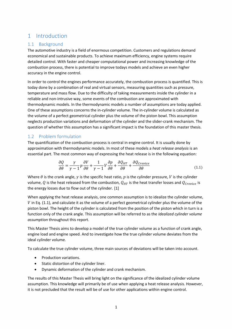
Figure 2.3. Relative impact of tolerances when components are pushed outwards from the combustion chamber

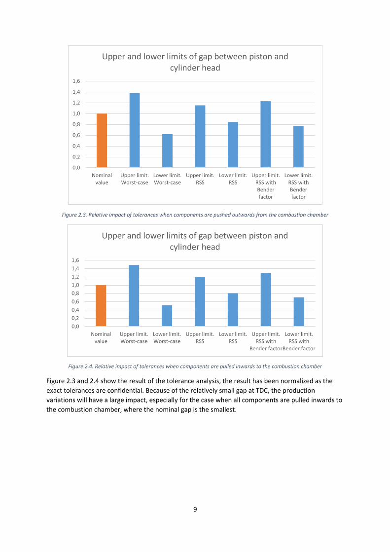
Figure 2.4. Relative impact of tolerances when components are pulled inwards to the combustion chamber

Figure 2.3 and 2.4 show the result of the tolerance analysis, the result has been normalized as the

exact tolerances are confidential. Because of the relatively small gap at TDC, the production

variations will have a large impact, especially for the case when all components are pulled inwards to

the combustion chamber, where the nominal gap is the smallest.

0,0

0,2

0,4

0,6

0,8

1,0

1,2

1,4

1,6

Nominalvalue

Upper limit.Worst-case

Lower limit.Worst-case

Upper limit.RSS

Lower limit.RSS

Upper limit.RSS withBenderfactor

Lower limit.RSS withBenderfactor

Upper and lower limits of gap between piston and cylinder head

0,0

0,2

0,4

0,6

0,8

1,0

1,2

1,4

1,6

Nominalvalue

Upper limit.Worst-case

Lower limit.Worst-case

Upper limit.RSS

Lower limit.RSS

Upper limit.RSS with

Bender factor

Lower limit.RSS with

Bender factor

Upper and lower limits of gap between piston and cylinder head

10

3 Theory of simulations In this chapter a brief summary of the underlying theory of the dynamic simulations will be

presented. The dynamic reduction and recovery is done in the FEM simulation software MSC

NASTRAN, and the multibody simulations are done in the software AVL Excite. For detailed theory,

the reader is referred to the theory manual of Nastran [11] and AVL Excite [12].

The purpose of the dynamic simulations is to investigate the structural behaviour of the crank-slider

mechanism as well as the cylinder head and cylinder liner when the components are exposed to the

forces associated with different operating points of the engine. With the deformations and

displacements known, the in-cylinder volume can be calculated with post-processing scripts. The

post-processing scripts will calculate the volume of only one of the six cylinders, but to obtain valid

results a full engine model is required.

3.1 Dynamic reduction The parts of the engine that are included in the model are described with FE-models. For each part

the corresponding mass matrix, 𝑴, dampening matrix, 𝑫, and stiffness matrix 𝑲, are generated. If 𝜽

is a vector containing all degrees of freedom (DOFs), the general equation of motion can be written

as:

𝑴 + 𝑫 + 𝑲𝜽 = 𝑭

Where 𝑭 is the applied loads. The full model, with all parts and corresponding degrees of freedom

will be very large, and to obtain a time based solution with fine resolution would be extremely

computational heavy. To solve this issue, a dynamic reduction is conducted to reduce the number of

DOFs in the system.

To understand the reduction process it is necessary to be familiar with the meaning of natural

frequencies and modal responses. A modal response represents a sinusoidal movement that

corresponds to a certain natural frequency of the system of DOFs. A system of DOFs always have the

same number of natural frequencies (and modal responses) as the number of DOFs. The natural

frequencies and corresponding mode can be obtained by solving the eigenvalue problem:

−Ω𝑝2𝑴 + 𝑖Ω𝑝𝑫 + 𝑲𝑩𝒑 = 𝟎

Where Ω𝑝 is the natural frequency and 𝑩𝒑 is the corresponding modal movement. If a system of

DOFs is subject to an external load that coincide with a natural frequency, the modal response is not

always high. If, for example, the external force is perpendicular to the modal movement, the

response will be zero. A scaling factor is defined for each mode, 𝑝, with the external load 𝑭𝑘 that has

the frequency 𝜔𝑘:

𝑞𝒌𝒑

=𝑩𝑝

𝑇𝑭𝑘

𝑚𝑚𝑜𝑑𝑎𝑙,𝑝(Ω𝑝2 − 𝜔𝑘

2) + 𝑖𝜔𝑘𝑑𝑚𝑜𝑑𝑎𝑙,𝑝

Where 𝑚𝑚𝑜𝑑𝑎𝑙,𝑝 = 𝑩𝑝𝑇𝑴𝑩𝑝 and 𝑑𝑚𝑜𝑑𝑎𝑙,𝑝 = 𝑩𝑝

𝑇𝑫𝑩𝑝.

The modal scaling factor, 𝑞𝑝, and the corresponding modal movements, 𝑩𝑝, will be important in the

dynamic reduction. The dynamic reduction is practically a change of base for the DOFs. The original

DOFs can be expressed in the reduced DOFs as:

𝜽 = 𝑪𝜶

(3.1)

(3.2)

(3.3)

(3.4)

11

Where 𝑪 is the change of base matrix and 𝜶 is the reduced DOFs. 𝑪 will have equally many rows as

the original number of DOFs and equally many columns as the reduced number of DOFs. The goal is

to find the solution with the reduced base that as close as possible satisfy the global energy balance.

The global energy is obtained by multiplying Eq. (3.1) from left with 𝑇 and integrating:

1

2𝑇𝑴 + ∫ 𝑇𝑫 𝑑𝑡 +

1

2𝜽𝑇𝑲𝜽 = ∫ 𝑇𝑭 𝑑𝑡

(3.5) corresponds to: Kinetic energy + dissipated energy + Strain energy = Applied energy. Expressed

in the reduced base the global energy balance becomes:

1

2𝑻𝑪𝑻𝑴𝑪 + ∫ 𝑻𝑪𝑻𝑫𝑪 𝑑𝑡 +

1

2𝜶𝑻𝑪𝑻𝑫𝑪𝜶 = ∫ 𝑻𝑪𝑻𝑭 𝑑𝑡

By comparing equations (3.4), (3.5) and (3.6) we can define the reduced system matrices as:

𝑴𝑟𝑒𝑑 = 𝑪𝑻𝑴𝑪 𝑫𝑟𝑒𝑑 = 𝑪𝑻𝑫𝑪 𝑲𝑟𝑒𝑑 = 𝑪𝑻𝑲𝑪 𝑭𝑟𝑒𝑑 = 𝑪𝑻𝑭

To determine 𝑪 the Craig-Bampton method is used. The original set of DOFs, 𝜽, is split into two sets

of DOFs, 𝜽𝐴 and 𝜽𝐵. 𝜽𝐴 includes the DOFs that are to be left after the reduction and 𝜽𝐵 are the DOFs

that are to be reduced. All DOFs that are subject to applied forces need to be included in 𝜽𝐴.

In addition to 𝜽𝐴 all modes that are to be included in the reduced model are saved in a set with the

corresponding scaling factor 𝒒. Typically the modes are limited at a certain frequency, so that the

modes corresponding to higher frequencies are neglected, as they contain a very small amount of

energy. The classic Craig-Bampton change of base matrix on block-matrix form is:

𝜽 = [𝜽𝐴

𝜽𝐵] = [

𝑰 𝟎𝑺 𝑩

] [𝜽𝐴

𝒒] = 𝑪𝐶𝐵𝜶

Where 𝑰 is the identity matrix and 𝑺 and 𝑩 are matrices that need to be determined. To determine

the matrices 𝑺 and 𝑩, equation (3.1) are rewritten in terms of 𝜽𝐴 and 𝜽𝐵, the dampening term is

here set to zero, but has normally the same form as the mass term.

[𝑴𝐴𝐴 𝑴𝐴𝐵

𝑴𝐵𝐴 𝑴𝐵𝐵] [

𝐴

𝐵

] + [𝑲𝐴𝐴 𝑲𝐴𝐵

𝑲𝐵𝐴 𝑲𝐵𝐵] [

𝜽𝐴

𝜽𝐵] = [

𝑭𝐴

𝟎]

𝑺 is the matrix that relates the physical displacements of 𝜽𝐵 to the displacements of 𝜽𝐴. By fixing the

modal DOFs and consider the static part of (3.9), 𝑺 can be determined:

𝑲𝐵𝐴𝜽𝐴 + 𝑲𝐵𝐵𝜃𝐵 = 𝟎 → 𝜽𝐵 = −𝑲𝐵𝐵−𝟏𝑲𝐵𝐴𝜽𝐴 → 𝑺 = −𝑲𝐵𝐵

−𝟏𝑲𝐵𝐴

𝑩 is the matrix that gives the physical displacements of 𝜽𝐵 that corresponds to the modal responses,

𝒒. By fixing the physical DOFs that are left after reduction, 𝜽𝐴, equation (3.9) and (3.8) reduces to:

𝑴𝐵𝐵𝐵 + 𝑲𝐵𝐵𝜽𝐵 = 𝟎 , 𝜽𝐵 = 𝑩𝒒

𝑺 and 𝑩 are now known and the reduction can be carried out, leaving the reduced system to be

solved:

𝑴𝑟𝑒𝑑 + 𝑫𝑟𝑒𝑑 + 𝑲𝑟𝑒𝑑𝜶 = 𝑭𝑟𝑒𝑑

(3.5)

(3.6)

(3.7)

(3.8)

(3.9)

(3.10)

(3.11)

(3.12)

12

Typically, an original set of over a million DOFs can be reduced to a couple of thousands. Saving a

considerable amount of computational capacity with a very small loss of accuracy. Once a solution

for the reduced system is found, the original full set of DOFs can be obtained by applying equation

(3.8).

3.2 Connecting rod and piston In the multibody simulations that has been done in this master thesis, the piston is assumed to be a

rigid body. This assumption was necessary given the resources available for this master thesis.

Another simplification that has been done in the multibody simulation is that the connecting rod is

modelled as a two-node bar element, instead of a reduced mesh. The mass of the piston is added to

the upper node of the connecting rod. These assumptions be discussed in Chapter 7.

3.3 Couplings of components When all components are dynamically reduced they are coupled to each other with different types of

joints. The joints can be hydrodynamic bearings, springs, gears and other types. The different types

of joints, and how they are modelled in AVL Excite can be read in the AVL Excite theory manual [12].

The radial bearings are modelled as non-linear spring-dampeners, that is approximating the

behaviour of the oil films in the bearings. The contact between the piston (in this model, the upper

node of the connecting rod) and the cylinder liner is modelled as a linear spring following a centreline

defined by the cylinder liner nodes. Figure 3.1 shows a block scheme view of the Excite model with all

components and joints.

Figure 3.1. Block scheme view of Excite model

13

4 Simulations and post-processing

4.1 Static deformations The static deformations of the cylinder include all deformations of the cylinder that does not directly

depend on time. Scania has been investigating the static deformations in detail. Investigations of

cylinder liner distortion have been done mainly with regard to cylinder friction, blow-by and oil

consumption [13], [14]. The results from these analyses include the distortion of the inner surface of

the cylinder and can therefore be used in this Master Thesis to determine the difference in volume

caused by the static deformations.

Because of the fact that the simulations are not included in the scope of this Master Thesis, the

theory behind them will be explained only briefly. However, the post-processing of the results from

the simulations was done in this Master Thesis and will thus be explained in more depth.

The static loads on the cylinder liner and cylinder head can be divided into two main categories, [14]:

Tension from the bolts that connects the cylinder head to the cylinder block and pins the

cylinder liner in position.

Thermal load from the heat distribution caused by the combustion.

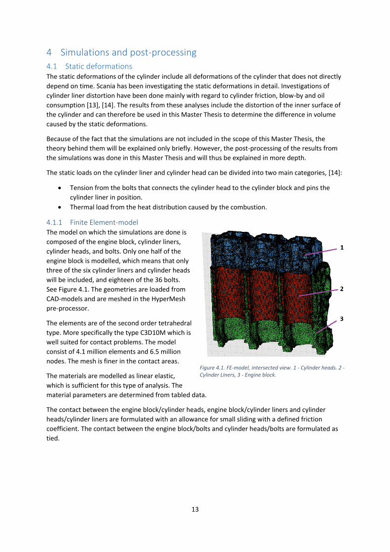
4.1.1 Finite Element-model The model on which the simulations are done is

composed of the engine block, cylinder liners,

cylinder heads, and bolts. Only one half of the

engine block is modelled, which means that only

three of the six cylinder liners and cylinder heads

will be included, and eighteen of the 36 bolts.

See Figure 4.1. The geometries are loaded from

CAD-models and are meshed in the HyperMesh

pre-processor.

The elements are of the second order tetrahedral

type. More specifically the type C3D10M which is

well suited for contact problems. The model

consist of 4.1 million elements and 6.5 million

nodes. The mesh is finer in the contact areas.

The materials are modelled as linear elastic,

which is sufficient for this type of analysis. The

material parameters are determined from tabled data.

The contact between the engine block/cylinder heads, engine block/cylinder liners and cylinder

heads/cylinder liners are formulated with an allowance for small sliding with a defined friction

coefficient. The contact between the engine block/bolts and cylinder heads/bolts are formulated as

tied.

Figure 4.1. FE-model, intersected view. 1 - Cylinder heads. 2 - Cylinder Liners, 3 - Engine block.

14

In Figure 4.2, a significant difference between the FE-model and the reality is highlighted. In the FE-model the top of the cylinder liners are in level with the top of the engine block. This is not the case in reality. The cylinder liners are actually in a level slightly above the engine block. The reason for this is that when the cylinder heads are mounted with the bolts to the engine block, the cylinder liner will receive a part of this tension and be pinned in place between the engine block and cylinder heads. This will cause the cylinder liner to deform. This deformation is referred to as cold cylinder liner distortion. In the FE-model, this gap is not included due to convergence issues. Instead the gap is included in the contact formulation between the cylinder heads and the cylinder liners, where it is defined as a negative clearance of δ mm (δ is the magnitude of this protrusion). In the deformed FE-model, the cylinder liners appear to be in a level beneath the engine block, but in reality they are in the same level. This has to be accounted for in the post-processing procedure.

4.1.2 Boundary conditions and loads The boundary conditions applied at the model are symmetry on the cut-through plane, and zero

displacement on nodes adjacent to the bearings (lower part of figure 4.1).

The tension from the bolts are included in the model as forces parallel to the respective bolt.

The heat distribution is dependent on the engine operating conditions. In this case the heat

distribution is simulated from a steady state engine operation at 1800 RPM and high reference load.

The CFD simulation is mapped onto the FE-model.

4.1.3 Finite element analysis Once the FE-model is completed according to the description above, the loads are applied. First the

tension from the bolts and secondly the thermal loads from the heat distribution. The analysis is

done in the Abaqus software.

4.1.4 Post-processing results The post-processing of the results from the FE-analysis has the purpose of calculating the in-cylinder

volume difference between the original geometry and the deformed geometry. All nodes on the

Figure 4.2. Illustration of difference between FE-model and reality, regarding cylinder liner overlap. All deformations are magnified.

15

inner surfaces of the cylinder liner and the cylinder head are exported from Abaqus. The result files

include original coordinates and displacements for each node.

The result file is loaded into MATLAB, where the post-processing will be done. Figure 4.3 – 4.4 show

how the surfaces adjacent to the in-cylinder volume is transferred to MATLAB.

First action of the post-processing script is to transform the nodal coordinates and displacements

from cartesian to cylindrical coordinates. First a coordinate origin is defined in the middle of the

original geometry of the cylinder liner, specifically somewhere along the centreline of the cylinder

liner. All coordinates are transformed to cylindrical coordinates according to:

𝑟 = √𝑥2 + 𝑦2

𝜃 = 𝑡𝑎𝑛−1 (𝑦

𝑥)

𝑧 = 𝑧

𝜃 = 𝜃 + 𝜋 𝑖𝑓 𝑥 < 0 𝑎𝑛𝑑 𝜃 = 𝜃 + 2𝜋 𝑖𝑓 𝜃 < 0

4.1.5 Volume calculation In order to calculate the volume of the original and deformed cylinder liner, a new uniform grid will

be defined, on which the grid from the result data will be mapped. The volume will be divided into

two zones (see Figure 4.5). The zones are separated by the z-value of a specific node. Before

deformation, all nodes on the upper border of the cylinder liner has the same z-value. During

deformation, the nodes will be displaced differently in upwards direction. The z-value of the node

that has been displaced the least amount will define the separation between the two zones. The

reason for this will be explained below.

Figure 4.3a. Cylinder liner, inner surface extracted and plotted in MATLAB (to the right)

Figure 4.3b. Deformed cylinder liner extracted and plotted in MATLAB (to the right). (Displacements magnified 500 times)

Figure 4.4a. Lower surface of cylinder head (called firedeck) extracted and plotted in MATLAB (to the right)

Figure 4.4b. Deformed firedeck extracted and plotted in MATLAB (to the right). (Displacements magnified 500 times)

(4.1)

16

Figur 4.5. Illustration of the upper and lower zones during volume calculation. Note that in reality the upper zone is around 0.02 mm thick and the lower zone is around 250 mm

4.1.5.1 Lower zone

In the lower zone, all nodes are fixed in angular and axial directions. To map the deformed grid from

the result file to the new defined grid, an interpolated surface is created in MATLAB. The surface is

defining the function 𝑟 = 𝑟(𝜃, 𝑧). The nodes are now spread uniformly in 𝑧- and 𝜃-directions, and the

r-direction depends on the deformation. This method makes the displacements in 𝑧- and 𝜃-directions

unknown, but as these displacement-directions do not have influence on the volume it is not a

concern. Only on the top boundary is the displacements in z-direction of importance. That is the

reason for dividing the volume into two zones. The z-displacements of the upper boundary are in

contact with the firedeck and will therefore be included when calculating the volume difference for

the displacements of the upper zone.

The volume of the lower zone can now be integrated using the trapezoidal method. The volume can

be expressed as:

𝑉 =1

2∬ 𝑟(𝜃, 𝑧)2𝑑𝜃𝑑𝑧

𝐴𝑠𝑢𝑟𝑓

= ∫ 𝐴(𝑧)𝑑𝑧

ℎ

0

𝑤ℎ𝑒𝑟𝑒 𝐴(𝑧) =1

2∫ 𝑟(𝜃, 𝑧)2𝑑𝜃

2𝜋

0

Where ℎ = 𝑧𝑚𝑎𝑥 − 𝑧𝑚𝑖𝑛. The volume can be determined numerically using the trapezoidal method

for the inner and outer integral according to:

𝐴(𝑧) =1

2∫ 𝑟(𝜃, 𝑧)2𝑑𝜃 =

∆𝜃

4∑(𝑟(𝜃𝑖+1, 𝑧)2 + 𝑟(𝜃𝑖, 𝑧)2)

𝑁𝑖

𝑖=1

2𝜋

0

𝑉 = ∫ 𝐴(𝑧)𝑑𝑧 =∆𝑧

2∑(𝐴(𝑧𝑗+1) + 𝐴(𝑧𝑗))

𝑁𝑗

𝑗=1

ℎ

0

Where 𝑁𝑖 is number of nodes in angular direction and ∆𝜃 = 2𝜋/𝑁𝑖. 𝑁𝑗 is the number of nodes in

axial direction and ∆𝑧 = ℎ/(𝑁𝑗 − 1).

4.1.5.2 Upper zone

In the upper zone, a uniform grid is defined with fixed nodes in radial and angular directions. A

surface is interpolated that defines the function 𝑧 = 𝑧(𝑟, 𝜃). The outer radius is defines as the mean

radius of the nodes on the top border of the lower zone.

(4.3)

(4.4)

(4.2)

17

The volume of the upper zone is calculated in a similar way as the lower zone. The difference is that

in this case the axial displacement is interpolated instead of the radial displacement. This will mean

that the radial displacement is unknown, and the top of the cylinder is assumed circular.

A uniform grid is defined with fixed nodes in radial and angular directions. A surface is interpolated

that defines the function 𝑧 = 𝑧(𝑟, 𝜃). The volume can now be calculated with the trapezoidal

method:

𝑉 = ∬ 𝑧(𝑟, 𝜃)𝑑𝐴 = ∑ ∑∆𝐴(𝑟𝑖,𝜃𝑗)

4[𝑧(𝑟𝑖, 𝜃𝑗) + 𝑧(𝑟𝑖+1, 𝜃𝑗) + 𝑧(𝑟𝑖, 𝜃𝑗+1) + 𝑧(𝑟𝑖+1, 𝜃𝑗+1)]

𝑁𝑗

𝑗=1𝑁𝑖𝑖=1𝐴𝑠𝑢𝑟𝑓

Where 𝑁𝑖 is the number of nodes in radial direction and 𝑁𝑗 is the number of nodes in angular

direction. ∆𝐴(𝑟𝑖, 𝜃𝑗) is the area of the element that is enclosed by 𝑟𝑖 , 𝑟𝑖+1 , 𝜃𝑗 and 𝜃𝑗+1.

∆𝐴(𝑟𝑖, 𝜃𝑗) =𝜃𝑗+1 − 𝜃𝑗

2(𝑟𝑖+1

2 − 𝑟𝑖2)

4.1.6 The ideal piston path During operation of the engine, the piston moves along the cylinder liner in the four strokes. During

the power stroke, the piston is forced downwards due to the high pressure in the combustion

chamber. The piston is connected to the connecting rod by the piston bolt, and the connecting rod is

connected to the crankshaft. When the piston is forced downwards, the crankshaft will rotate, see

Figure 4.6. This system of components is called the slider-crank mechanism.

Figure 4.6. Schematic illustration of the slider-crank mechanism. 𝑙 notes the connecting rod, r notes the crankpin, s is the stroke length, and x is the distance from TDC to the top of the connecting rod.

It is necessary to relate the linear movement of the piston to the rotation of the crankshaft. From Figure 4.6 it can be derived that the distance, 𝑥, from TDC to the small end of the connecting rod can be expressed in terms of α, [15]:

𝑥(𝛼) = 𝑟 (1 − cos(𝛼) +1

λ(1 − √1 − λ2𝑠𝑖𝑛2(𝛼)))

Where 𝛼 is the crank angle, r is the crank radius, λ is the ratio between the crank radius and the

length of the connecting rod; λ =𝑟

𝑙. All these quantities are noted in Figure 4.6.

(4.5)

(4.6)

(4.7)

18

Figure 4.7. The ideal piston path

Figure 4.7 shows a plot of Eq. (4.7). This path will in this report be called the ideal piston path.

4.1.7 The compensated piston path In the FE-model used to analyse the static deformations, only the components listed in section 4.1.1

are included. What is lacking in this model is the crank-slider mechanism. When the engine is heated

up, the parts of the crank-slider mechanism will also be heated up. It is of importance to understand

how the parts of the crank-slider mechanism will expand as this will have an influence on the in-

cylinder volume.

In this master thesis the expansion of the components of the slider-crank mechanism will be

approximated analytically. The length of the crank radius, the connecting rod and the piston will be

considered. As the pressure inside the cylinder and the inertia forces will be analysed later, the

thermal expansions of these magnitudes will be treated as one-dimensional free thermal expansions,

and calculated using the free thermal strain, [16]:

𝜖 = 𝛼∆𝑇

Where 𝜖 is the non-dimensional normal strain defined as 𝜖 =𝑙−𝑙0

𝑙0. 𝑙0 is the original length and 𝑙 is

the length after the thermal expansion. 𝛼 is a material constant called the coefficient of linear

thermal expansion with the unit [1

°𝐶]. ∆𝑇 is the difference in temperature from the reference

temperature for which the length is 𝑙0 (in this case 20°𝐶), the unit of ∆𝑇 is [°𝐶].

With the approximated length of the magnitudes a new compensated piston path can be calculated.

The volume of the combustion chamber after the cold and the warm distortion can now be

calculated as a function of crank angle. The results are presented in Chapter 5.

4.1.7.1 Approximation of temperatures in the slider-crank mechanism

The crank shaft is approximated to have the same temperature as the oil surrounding it. The oil

temperature measured at the operating point of 1900 RPM and high reference load is 107.8°𝐶. This

operating point is not exactly the one that is simulated, which is – as mentioned in section 4.1.2 –

1800 RPM and high reference load. But as measured data is lacking for the simulated operating

point, this data is considered sufficiently accurate.

The temperature measured below the first ring groove in the piston is around 175°𝐶. This

temperature is measured – like the oil temperature – at the operating point of 1900 RPM and high

load.

(4.8)

19

The temperature will in this analysis be approximated to vary linearly from the measuring point on

the piston down to the crank shaft. This approximation should be sufficient for this analysis.

The coefficient of linear thermal expansion, 𝛼, is gathered from tabled data in [17]. For the piston,

which is made of steel , 𝛼 have the value of 1310−6𝑚

𝑚∗𝐾. The materials of the crank shaft and the

connecting rod are made of similar compositions and will here be assumed to have the same 𝛼 as the

piston.

The average temperatures for the components together with corresponding thermal expansions are

listed in table 4.1.

Component Dimension Approximated temperature

Original length Length after thermal expansion

Crank shaft Crank radius 108°𝐶 80 mm 80.1 mm

Connecting rod Length of connecting rod

116°𝐶 255 mm 255.3 mm

Piston Length of piston 170°𝐶 82 mm 82.4 mm Table 4.1. Results of analytical approximation of thermal expansion of slider-crank mechanism.

These results will define the compensated piston path which is used to approximate the volume

difference over the scope of one engine rotation (360 degrees).

4.2 Dynamic deformations The dynamic deformations are calculated in a dynamically reduced model of the engine. The theory

behind the model is presented in Chapter 3. In this section it will be explained how the loads are

applied on the model and results are gathered. The results will be presented in chapter 5.

4.2.1 External loads on model The external loads on the model will consist of the pressure traces of cylinder one and six. Because of

phenomena such as torsion of the crankshaft, the pressure traces will differ in the six cylinders [4]. As

cylinder six is closest to the flywheel where the power is taken out of the engine, and cylinder one is

furthest away from the flywheel, these two cylinders will represent the extreme cases of the

difference in the pressure traces. The influence from the torsion of the crankshaft will be smallest at

cylinder six [4] and will therefore be in focus during this master thesis.

The pressure trace that is used as input to the Excite model is taken from measurements during the

experimental phase of a previous master thesis work at Scania, the procedure is described in [4].

4.2.2 Post-processing the results from the displacement of the connecting rod The results from the simulation are extracted in form of the displacements of the nodes of the

model. The nodes are illustrated in figure 4.8. Each node has six degrees of freedom, three

translational and three rotational.

20

Figure 4.8. Schematic illustrations of the nodes of interest when analysing the displacements of the crank-slider mechanism.

For each of the six operating points and for each crank angle degree, the displacements of these

nodes are saved. With the information of the nodal displacements, the deformations can be related

to the forces acting on the nodes. This will be done in Chapter 6, when the final model is established.

Eventually, the node of interest to calculate the in-cylinder volume is node 5, because of the fact that

the piston is considered a rigid body in the multibody simulation model, node 5 will – together with

an offset representing the piston height – define the bottom of the combustion chamber.

4.2.3 Post-processing the results of the displacements of the cylinder head The top side of the cylinder is defined by 133 nodes. These nodes form a surface that is originally flat,

but when exposed to the high in-cylinder pressure will deform outwards, making the in-cylinder

volume larger. This section will explain how the deformed volume is calculated.

The set of nodes defining the top of the cylinder is gathered from the recovery of the FE-model

explained in Chapter 3. For each node, the original coordinates as well as the displacements for every

degree of crank angle are known.

Figure 4.9. Original and displaced nodes of the inner surface of the cylinder liner. Displacements in the right figure are magnified 1000 times.

Figure 4.9 shows the nodes that are defining the inner surface of the cylinder, the original nodal

coordinates to the left and the displaced nodal coordinates to the right, with the displacements

magnified 1000 times. It is visible how the top of the cylinder is deformed outwards, as expected,

due to the high pressure in the cylinder. It is also visible that the cylinder liner has a protrusion to the

left, this is due to the force of the piston acting on the cylinder liner close to TDC. The last

observation that can be made from Figure 4.11, is the fact that the whole cylinder is tilting. This is

due to the rigid body motion of the engine against the engine suspension. The reciprocating masses

21

and rotating shafts in the engine, will cause the engine to vibrate. In the current state of Figure 4.10

the engine block is tilting slightly to the left. To calculate the volume increase due to the deformation

of the cylinder top, the rigid body motions need to be excluded.

To find, and eventually filter out, the rigid body motions, a centreline of the cylinder will be defined.

The centreline will be defined by the displacements of the nodes that are not exposed to pressure

forces, in other words, the nodes that are purely displaced due to the rigid body motion. These nodes

will be the nodes on the bottom half of the cylinder liner.

Once the centreline is defined and is following the rigid body motion, the displaced nodes on the top

of the cylinder is orthogonally projected on the centreline. This way, the pure deformation of the

cylinder top can be extracted from the displacements and no longer include the rigid body

movement. Using Matlab, a surface is interpolated over the nodes of the top of the cylinder, see

Figure 4.10.

Figure 4.10. Interpolated surface over the nodes defining the top of the cylinder. Displacements are magnified 30 times.

The interpolated surface is made of a net of 33x33 squares. By taking the average z-coordinate of the

square and the area of the squares, the volume under the surface can be approximated with

satisfying accuracy. The results of this analysis is presented in Chapter 5.

22

5 Results of simulations

5.1 Volume difference due to cold liner distortion Before the cylinder head is mounted on the cylinder block during assembly, the cylinder liner has a

small protrusion over the cylinder block. When the cylinder block is mounted and fixed with the six

bolts per cylinder, the top of the cylinder liner is forced to the same level as the top of the cylinder

block. This will leave a residual tension in the assembly that will deform the components. The

deformation is referred to as cold liner distortion, as it is in effect even when the engine is cold.

Using the post-processing script described in part 4.1.5 the volume of the cylinder is calculated. As

neither the crankshaft, the connecting rod, the piston bolt or the piston is affected by the cold liner

distortion, the piston is assumed to follow its ideal path. The ideal path is explained in section 4.1.6.

The result of the cold distortion is here presented in two plots, the first plot presents the absolute

difference in volume over one engine cycle and the second plot represents the percentage difference

in volume over one engine rotation.

Figure 5.1. Absolute volume difference due to cold liner distortion, where 100 % is the undeformed result. TDC at 0 and 360 degrees and BDC at 180 degrees.

Figure 5.2. Relative volume difference due to cold liner distortion. TDC at 0 and 360 degrees and BDC at 180 degrees.

23

The absolute difference shows that the largest difference in absolute volume between the deformed

cylinder and the non-deformed cylinder is located at BDC (±180°). This is because the cold distortion

makes the cylinder radius slightly larger, and the cylinder will have the largest surface area at BDC. It

is also worth noting that there is an absolute volume increase at TDC, this is because the cylinder

head has deformed slightly which has increased the dead volume.

The relative difference in volume will, contrary to the absolute difference, be smallest at BDC. This is

because even though the absolute difference is largest here, the total cylinder volume will also be at

its largest, and the absolute difference will have a very small impact.

5.2 Volume difference due to hot distortion When the engine is operating, it will become warm and cause all components to expand. Along with

the description in section 4.1 this has been simulated.

As described in section 4.1.7, the slider-crank mechanism is not included in the simulation and has

therefore been approximated analytically. The results of these approximations are presented in

Table 4.1.

The results of this simulation is presented below in the same way as for the cold distortion.

Figure 5.3. Absolute volume difference due to hot liner distortion, where 100 % is the undeformed result.. TDC at 0 and 360 degrees and BDC at 180 degrees.

Figure 5.4. Relative volume difference due to hot liner distortion. TDC at 0 and 360 degrees and BDC at 180 degrees.

24

What is most interesting to note is the fact that the deformed volume becomes smaller than the non-

deformed volume, when the piston is between ±70° from TDC. The percentage difference is largest

at TDC. This is because the components of the slider-crank mechanism expand more than the engine

block, according to the analytical approximation explained in 4.2.7.

5.3 Volume increase due to displacement of piston In this section the results from the dynamic simulations will be presented as the total volume

displacement caused by the displacement of the piston, over an engine cycle for different operating

points.

Figure 5.5. Absolut volume displacement as a function of crank angle degree

Figure 5.5 shows the absolute volume displacement over one cycle for three different operating

points. For most of the cycle, the upper node of the connecting rod is displaced in negative direction,

which results in an absolute volume increase of the combustion chamber compared to the ideal

piston path. The relative volume increase can be seen in Figure 5.6.

Figure 5.6. Relative volume displacement in percent. Displaced volume/ideal volume

25

The relative volume increase is a comparison between the volume calculated with the displaced

piston and the volume calculated with the ideal piston path.

5.4 Volume increase due to deformation of cylinder head In this section the results from the dynamic simulations will be presented as the total volume

displacement caused by the deformation of the cylinder head, over a range of crank angle degree for

different operating points.

The fine mesh necessary to calculate the displaced volume due to deformation of the cylinder head,

was only recovered for a CAD range of TDCc±30°. It can be concluded that the volume displacement

due to deformation of the cylinder head is small compared to the volume displaced due to

displacement of the piston.

Figure 5.7. Absolute volume displacement due to deformation of the cylinder head

26

6 Model The objective of the model is to combine all results from the simulations to create a model that

based on the in-cylinder pressure, the crank angle degree and the engine speed can estimate the in-

cylinder volume. As the eventual purpose of the model is to be implemented in the Electrical Control

Unit on board a vehicle, with limited computational capacity, the model will calculate the volume

without iterating and without solving nonlinear differential equations.

In Chapter 5 all displacements that contribute to the volume change are summarised. The first step

of creating the model is to formulate relations between the displacements and the in-parameters.

These relations will be based on the physical constitutive relations that can be found in literature.

The model will be created with a grey box approach, so that when the displacements seen in the

simulations cannot be explained satisfactory with only the in-parameters, those will be

complimented with reasonable assumptions. Whenever this is the case, it will be stated clearly.

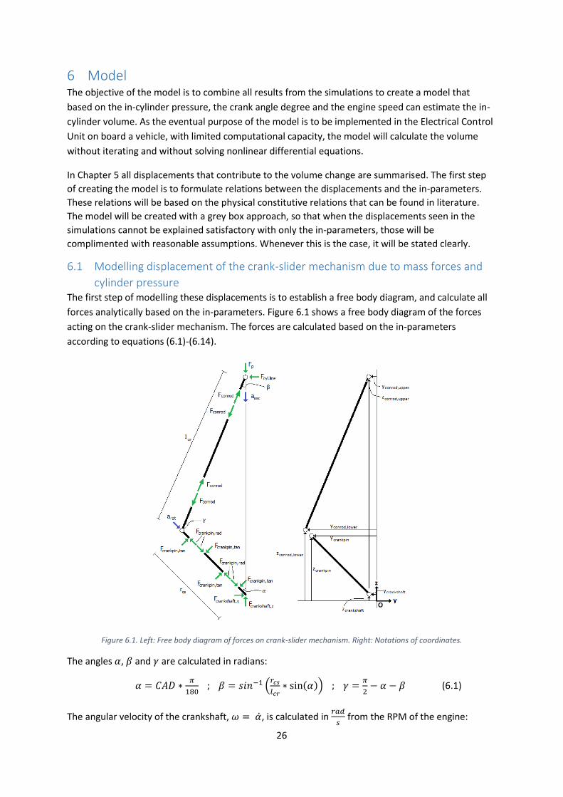
6.1 Modelling displacement of the crank-slider mechanism due to mass forces and

cylinder pressure The first step of modelling these displacements is to establish a free body diagram, and calculate all

forces analytically based on the in-parameters. Figure 6.1 shows a free body diagram of the forces

acting on the crank-slider mechanism. The forces are calculated based on the in-parameters

according to equations (6.1)-(6.14).

Figure 6.1. Left: Free body diagram of forces on crank-slider mechanism. Right: Notations of coordinates.

The angles 𝛼, 𝛽 and 𝛾 are calculated in radians:

𝛼 = 𝐶𝐴𝐷 ∗𝜋

180 ; 𝛽 = 𝑠𝑖𝑛−1 (

𝑟𝑐𝑠

𝑙𝑐𝑟∗ sin(𝛼)) ; 𝛾 =

𝜋

2− 𝛼 − 𝛽 (6.1)

The angular velocity of the crankshaft, 𝜔 = , is calculated in 𝑟𝑎𝑑

𝑠 from the RPM of the engine:

27

𝜔 = 𝑅𝑃𝑀 ∗2𝜋

60 (6.2)

The forces and accelerations are calculated based on the angles, engine speed and cylinder pressure:

𝐹𝑝 = 𝑃𝑐𝑦𝑙 ∗ 𝐴𝑝𝑖𝑠𝑡 (6.3)

Where 𝐴𝑝𝑖𝑠𝑡 is the area of the piston facing the combustion chamber.

𝐹𝑜𝑠𝑐 = 𝑚𝑜𝑠𝑐𝑎𝑜𝑠𝑐 (6.4)

𝑎𝑜𝑠𝑐 = −𝑟𝑐𝑠(𝜔2 ∗ cos(𝛼) +𝑟𝑐𝑠

𝑙𝑐𝑟∗ 𝜔2 ∗ cos(2 ∗ 𝛼)) (6.5)

𝐹𝑟𝑜𝑡 = 𝑚𝑟𝑜𝑡𝑎𝑟𝑜𝑡 (6.6)

𝑎𝑟𝑜𝑡 = −𝑟𝑐𝑠 ∗ 𝜔2 (6.7)

𝐹𝑐𝑜𝑛𝑟𝑜𝑑,𝑧 = 𝐹𝑜𝑠𝑐 − 𝐹𝑝 (6.8)

𝐹𝑐𝑜𝑛𝑟𝑜𝑑 =𝐹𝑐𝑜𝑛𝑟𝑜𝑑,𝑧

cos(𝛽) (6.9)

𝐹𝑐𝑜𝑛𝑟𝑜𝑑,𝑦 = 𝐹𝑐𝑜𝑛𝑟𝑜𝑑 ∗ sin(𝛽) (6.10)

𝐹𝑐𝑟𝑎𝑛𝑘𝑝𝑖𝑛,𝑟𝑎𝑑 = 𝐹𝑟𝑜𝑡 + 𝐹𝑐𝑜𝑛𝑟𝑜𝑑 ∗ sin(𝛾) (6.11)

𝐹𝑐𝑟𝑎𝑛𝑘𝑝𝑖𝑛,𝑡𝑎𝑛 = 𝐹𝑐𝑜𝑛𝑟𝑜𝑑 ∗ cos(𝛾) (6.12)

𝐹𝑐𝑟𝑎𝑛𝑘𝑠ℎ𝑎𝑓𝑡,𝑧 = 𝐹𝑐𝑟𝑎𝑛𝑘𝑝𝑖𝑛,𝑟𝑎𝑑 ∗ cos(𝛼) + 𝐹𝑐𝑟𝑎𝑛𝑘𝑝𝑖𝑛,𝑡𝑎𝑛 ∗ sin(𝛼) (6.13)

𝐹𝑐𝑟𝑎𝑛𝑘𝑠ℎ𝑎𝑓𝑡,𝑦 = −𝐹𝑐𝑟𝑎𝑛𝑘𝑝𝑖𝑛,𝑟𝑎𝑑 ∗ sin(𝛼) + 𝐹𝑐𝑟𝑎𝑛𝑘𝑝𝑖𝑛,𝑡𝑎𝑛 ∗ cos(𝛼) (6.14)

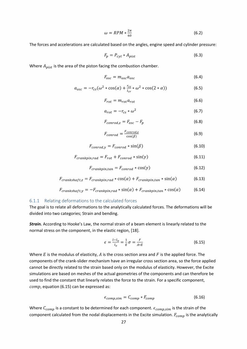
6.1.1 Relating deformations to the calculated forces The goal is to relate all deformations to the analytically calculated forces. The deformations will be

divided into two categories; Strain and bending.

Strain. According to Hooke’s Law, the normal strain of a beam element is linearly related to the

normal stress on the component, in the elastic region, [18].

𝜖 =𝑙−𝑙𝑜

𝑙𝑜=

1

𝐸𝜎 =

𝐹

𝐴∗𝐸 (6.15)

Where 𝐸 is the modulus of elasticity, 𝐴 is the cross section area and 𝐹 is the applied force. The

components of the crank-slider mechanism have an irregular cross section area, so the force applied

cannot be directly related to the strain based only on the modulus of elasticity. However, the Excite

simulations are based on meshes of the actual geometries of the components and can therefore be

used to find the constant that linearly relates the force to the strain. For a specific component,

𝑐𝑜𝑚𝑝, equation (6.15) can be expressed as:

𝜖𝑐𝑜𝑚𝑝,𝑠𝑖𝑚 = 𝐶𝑐𝑜𝑚𝑝 ∗ 𝐹𝑐𝑜𝑚𝑝 (6.16)

Where 𝐶𝑐𝑜𝑚𝑝 is a constant to be determined for each component. 𝜖𝑐𝑜𝑚𝑝,𝑠𝑖𝑚 is the strain of the

component calculated from the nodal displacements in the Excite simulation. 𝐹𝑐𝑜𝑚𝑝 is the analytically

28

calculated force on the component, from equations (6.1) to (6.14).

Figure 6.2. Bending of beam

Bending. According to the Bernoulli beam theory, the deflection of a beam that is anchored in one

end and loaded perpendicular in the other end, see Figure 6.2, can be described by, [18]:

𝑤 = 𝐹∗𝐿3

3∗𝐸∗𝐼 (6.17)

The deflection, 𝑤, is related to the angle, 𝛿, as sin(𝛿) =𝑤

𝑙, see Figure 6.2. As 𝑤 will be small

compared to 𝑙𝑐𝑠 , the following approximation can be done: 𝛿 ≈ sin (𝛿). Equation (6.17) can be

expressed as:

𝛿𝑐𝑜𝑚𝑝,𝑠𝑖𝑚 ≈ 𝐶𝑐𝑜𝑚𝑝 ∗ 𝐹𝑐𝑜𝑚𝑝 (6.18)

Where 𝐶𝑐𝑜𝑚𝑝 is a constant to be determined for each component. 𝛿𝑐𝑜𝑚𝑝,𝑠𝑖𝑚 is the angular bending

of the component, calculated from the nodal displacements in the Excite simulation. 𝐹𝑐𝑜𝑚𝑝 is the

analytically calculated force on the component, from equations (6.1) to (6.14).

The constants that relates the deformations to the analytical forces will now be determined for each

of the components.

Strain of the connecting rod. The strain of the connecting rod can be calculated from the

displacements of nodes 4 and 5 as defined in Figure 4.8. The relation between 𝐹𝑐𝑜𝑛𝑟𝑜𝑑 and

𝜖𝑐𝑜𝑛𝑟𝑜𝑑,𝑠𝑖𝑚 is plotted in Figure 6.3.

Figure 6.3. Deformation of connecting rod

The result shows a perfectly linear relation between the analytically calculated force and the strain in

the Excite simulation. For the connecting rod, Equation (6.16) is written as:

29

𝜖𝑐𝑜𝑛𝑟𝑜𝑑,𝑠𝑖𝑚 = 𝐶𝑐𝑜𝑛𝑟𝑜𝑑 ∗ 𝐹𝑐𝑜𝑛𝑟𝑜𝑑 (6.19)

With the data presented in Figure 6.3, 𝐶𝑐𝑜𝑛𝑟𝑜𝑑 can be determined.

Strain of crankpin. The strain of the crankpin can be calculated from the displacements of nodes 1, 2

and 3, as defined in Figure 4.8. The relation between 𝐹𝑐𝑟𝑎𝑛𝑘𝑝𝑖𝑛,𝑟𝑎𝑑 and 𝜖𝑐𝑟𝑎𝑛𝑘𝑝𝑖𝑛,𝑠𝑖𝑚 is plotted in

Figure 6.4.

Figure 6.4. Radial deformation of crankpin

The relation between the force and the strain is not perfectly linear and differs between the

operating points. On the left plot in Figure 6.4, an oscillation can be seen that cannot be related to

the force. This is likely due to the fact that the length of the crankpin is calculated from two different

nodes on the crankshaft, and as the crankshaft is subjected to bending and torsion, the length of the

crankpin appears to oscillate. With a relatively small error the relation between the strain and the

force can be approximated to be linear. For the crankpin, Equation (6.16) is written as:

𝜖𝑐𝑟𝑎𝑛𝑘𝑝𝑖𝑛,𝑠𝑖𝑚 = 𝐶𝑐𝑟𝑎𝑛𝑘𝑝𝑖𝑛,𝑟𝑎𝑑 ∗ 𝐹𝑐𝑟𝑎𝑛𝑘𝑝𝑖𝑛,𝑟𝑎𝑑 (6.20)

𝐶𝑐𝑟𝑎𝑛𝑘𝑝𝑖𝑛,𝑟𝑎𝑑 is determined to fit the simulated data as accurately as possible.

Bending of crankpin. The bending of the crankpin can be calculated from the displacements of nodes

1, 2 and 3, as defined in Figure 4.8. The relation between 𝐹𝑐𝑟𝑎𝑛𝑘𝑝𝑖𝑛,𝑡𝑎𝑛 and 𝛿𝑐𝑟𝑎𝑛𝑘𝑝𝑖𝑛,𝑠𝑖𝑚 is plotted in

Figure 6.5.

30

Figure 6.5. Bending of crankpin

It is noted that the relation between the angular bending and the tangential force in this case is far

from linear. In the left plot in Figure 6.5 it can be seen that the tangential displacement has not one

clear peek corresponding the analytically calculated tangential force, it has peeks repeating exactly

every 120 degrees. It is assumed that these peeks in angular bending can be explained with the

torsion of the crankshaft that occurs during the combustion in the other five cylinders. To account for

this, the tangential force is calculated not once as originally intended, but six times with an offset of

120 degrees for each calculation and with the corresponding in-cylinder pressure. The tangential

force acting on the crankpin will be the sum of these calculated forces, where each of the five

contributing tangential forces are scaled with a factor depending on how much it should influence

the resulting tangential force. For the bending of the crankpin, Equation (6.18) is written as:

𝛿𝑐𝑟𝑎𝑛𝑘𝑝𝑖𝑛,𝑠𝑖𝑚 ≈ 𝐶𝑐𝑟𝑎𝑛𝑘𝑝𝑖𝑛,𝑡𝑎𝑛 ∗ 𝐹𝑐𝑟𝑎𝑛𝑘𝑝𝑖𝑛,𝑡𝑎𝑛𝑟𝑒𝑠 (6.21)

Where 𝐹𝑐𝑟𝑎𝑛𝑘𝑝𝑖𝑛,𝑡𝑎𝑛𝑟𝑒𝑠 is the resultant tangential force after adding the influence of the other five

cylinders:

𝐹𝑐𝑟𝑎𝑛𝑘𝑝𝑖𝑛,𝑡𝑎𝑛𝑟𝑒𝑠 = 𝐹𝑐𝑟𝑎𝑛𝑘𝑝𝑖𝑛,𝑡𝑎𝑛 + ∑ 𝐶𝑖𝑛𝑓𝑙𝑢𝑒𝑛𝑐𝑒

𝑐𝑦𝑙∗ 𝐹𝑐𝑟𝑎𝑛𝑘𝑝𝑖𝑛,𝑡𝑎𝑛

𝑐𝑦𝑙5𝑐𝑦𝑙=1 (6.22)

Where 𝐹𝑐𝑟𝑎𝑛𝑘𝑝𝑖𝑛,𝑡𝑎𝑛𝑐𝑦𝑙

is the tangential force calculated with an angular offset for each cylinder with

the corresponding in-cylinder pressure. 𝐶𝑖𝑛𝑓𝑙𝑢𝑒𝑛𝑐𝑒𝑐𝑦𝑙

is a factor determining how much influence each

cylinder will have on the resultant tangential force. The result of this approach is shown in Figure 6.6.

31

Figure 6.6. Bending of crankpin with 6-cylinder contribution

In the left plot of Figure 6.6, it can be seen that the behaviour of the Excite simulation are captured

when adding the force from the other five cylinders. The corresponding force-displacement relation

(seen in the right plot of Figure 6.6) can now be assumed to be linear and is approximated with Eq.

(6.21) and (6.22), the constants are determined to fit the Excite simulation data as well as possible.

Displacement of top of connecting rod in y-direction. The displacement of the top of the connecting

rod in y-direction will be considered linearly related to the force in y-direction.

∆𝑦 = 𝐶𝑐𝑜𝑛𝑟𝑜𝑑,𝑡𝑜𝑝,𝑦 ∗ 𝐹𝑐𝑜𝑛𝑟𝑜𝑑,𝑦 (6.23)

Where 𝐶𝑐𝑜𝑛𝑟𝑜𝑑,𝑡𝑜𝑝,𝑦 is a constant that is determined based on data from Excite simulations. Figure

6.7 shows the relation.

Figure 6.7. Displacement of top of the connecting rod in y-direction.

The operating point of 1900 RPM high reference load is deviating significantly from the other

operating points. The probable cause for this is that the analytical force is not calculated correctly

because the angle 𝛽, is wrongly approximated. The displacements alter the forces, and the

32

calculations does not account for this, as it would require iterating. This error is expected to be larger

when the engine speed is higher, as the inertia forces will be larger. The error will eventually be of

small significance, as the y-displacement of the connecting rod is not greatly influencing the z-

displacement of the connecting rod. Also, the magnitudes of the displacements in y-direction that

reach almost 1.5 mm, are not reasonable. It would indicate that the stiffness of the cylinder wall

probably is too low in the simulations. This will be discussed in Chapter 7.

Radial bearings. The radial bearings on the connections between the crankshaft and the cylinder

block (main bearing) and the crankshaft and the connecting rod (big end bearing) will be modelled as

if the shafts move freely in the radial clearings.

∆𝑧 =𝐹𝑧

𝐹𝑡𝑜𝑡∗ 𝜇𝑚𝑏 ; ∆𝑦 =

𝐹𝑦

𝐹𝑡𝑜𝑡∗ 𝜇𝑚𝑏 (6.24a ; 6.24b)

Where 𝐹𝑡𝑜𝑡is the total force acting on the shaft. 𝐹𝑧 and 𝐹𝑦 are the z- and y-component of 𝐹𝑡𝑜𝑡. 𝜇𝑚𝑏 is

the radial clearance for the main bearing. The radial clearance for the big end bearing is exactly the

same, with the radial clearance 𝜇𝑏𝑒. Figure 6.8 and 6.9 shows plots of the z- and y-displacements of

the shafts in the main bearing and the big end bearing compared to the Excite simulations.

Figure 6.8. Radial clearance main bearing

Figure 6.9. Radial clearance big end bearing

In the Excite simulation, the contact between the shafts and the holes are modelled as non-linear

33

spring-dampeners, to capture the oil film behaviour. The approach of this model, where the shafts

move freely in the holes, neglects the oil film behaviour. This simplification is necessary to avoid

solving non-linear differential equations, which would be time consuming and interfere with the

purpose of the model. In the model, the magnitude of the force has no influence on the

displacement of the shaft, only the direction of the force determines the displacement. Close to TDCc

the magnitude of the force is large, and for the Excite simulation, it is visible how the shaft is

displaced downwards due to this, while in the model, it is on the same level as before because the

direction of the force has not changed. Another difference is the oscillating behaviour of the Excite

simulation on the main bearing. This is caused by torsion and bending of the crankshaft.

6.1.2 Position of the piston in z-direction Once the deformations of the connecting rod and the crankpin is approximated along with the radial

clearances, the position of the top of the connecting rod can be calculated.

𝑧𝑐𝑟𝑎𝑛𝑘𝑠ℎ𝑎𝑓𝑡 = −𝐹𝑐𝑟𝑎𝑛𝑘𝑠ℎ𝑎𝑓𝑡,𝑧

𝐹𝑐𝑟𝑎𝑛𝑘𝑠ℎ𝑎𝑓𝑡∗ 𝜇𝑚𝑏 ; 𝑦𝑐𝑟𝑎𝑛𝑘𝑠ℎ𝑎𝑓𝑡 = −

𝐹𝑐𝑟𝑎𝑛𝑘𝑠ℎ𝑎𝑓𝑡,𝑦

𝐹𝑐𝑟𝑎𝑛𝑘𝑠ℎ𝑎𝑓𝑡∗ 𝜇𝑚𝑏

𝑟𝑐𝑠 = 𝐹𝑐𝑟𝑎𝑛𝑘𝑝𝑖𝑛,𝑟𝑎𝑑 ∗ 𝐶𝑐𝑟𝑎𝑛𝑘𝑝𝑖𝑛,𝑟𝑎𝑑 ∗ 𝑟𝑐𝑠,0 + 𝑟𝑐𝑠,0

𝛿𝑐𝑟𝑎𝑛𝑘𝑝𝑖𝑛,𝑡𝑎𝑛 = 𝐹𝑐𝑟𝑎𝑛𝑘𝑝𝑖𝑛,𝑡𝑎𝑛 ∗ 𝐶𝑐𝑟𝑎𝑛𝑘𝑝𝑖𝑛,𝑡𝑎𝑛

𝑧𝑐𝑟𝑎𝑛𝑘𝑝𝑖𝑛 = 𝑧𝑐𝑟𝑎𝑛𝑘𝑠ℎ𝑎𝑓𝑡 + 𝑟𝑐𝑠 ∗ cos (𝛼 + 𝛿𝑐𝑟𝑎𝑛𝑘𝑝𝑖𝑛,𝑡𝑎𝑛)

𝑦𝑐𝑟𝑎𝑛𝑘𝑝𝑖𝑛 = 𝑦𝑐𝑟𝑎𝑛𝑘𝑠ℎ𝑎𝑓𝑡 + 𝑟𝑐𝑠 ∗ sin (𝛼 + 𝛿𝑐𝑟𝑎𝑛𝑘𝑝𝑖𝑛,𝑡𝑎𝑛)

𝑧𝑐𝑜𝑛𝑟𝑜𝑑,𝑙𝑜𝑤𝑒𝑟 = 𝑧𝑐𝑟𝑎𝑛𝑘𝑝𝑖𝑛 −𝐹𝑐𝑜𝑛𝑟𝑜𝑑,𝑧

𝐹𝑐𝑜𝑛𝑟𝑜𝑑∗ 𝜇𝑏𝑒

𝑦𝑐𝑜𝑛𝑟𝑜𝑑,𝑙𝑜𝑤𝑒𝑟 = 𝑦𝑐𝑟𝑎𝑛𝑘𝑝𝑖𝑛 −𝐹𝑐𝑜𝑛𝑟𝑜𝑑,𝑦

𝐹𝑐𝑜𝑛𝑟𝑜𝑑∗ 𝜇𝑏𝑒

𝑙𝑐𝑟 = 𝐹𝑐𝑜𝑛𝑟𝑜𝑑 ∗ 𝐶𝑐𝑜𝑛𝑟𝑜𝑑 ∗ 𝑙𝑐𝑟,0 + 𝑙𝑐𝑟,0

𝑦𝑐𝑜𝑛𝑟𝑜𝑑,𝑦𝑝𝑝𝑒𝑟 = 𝐹𝑐𝑜𝑛𝑟𝑜𝑑,𝑦 ∗ 𝐶𝑐𝑜𝑛𝑟𝑜𝑑,𝑡𝑜𝑝,𝑦

𝑧𝑐𝑜𝑛𝑟𝑜𝑑,𝑢𝑝𝑝𝑒𝑟 = 𝑧𝑐𝑜𝑛𝑟𝑜𝑑,𝑙𝑜𝑤𝑒𝑟 + √𝑙𝑐𝑟2 − (𝑦𝑐𝑜𝑛𝑟𝑜𝑑,𝑢𝑝𝑝𝑒𝑟 − 𝑦𝑐𝑜𝑛𝑟𝑜𝑑,𝑙𝑜𝑤𝑒𝑟)

2

Together with the length of the piston, 𝑧𝑐𝑜𝑛𝑟𝑜𝑑,𝑢𝑝𝑝𝑒𝑟 defines the bottom surface of the cylinder. The

results of the model can now be compared with the results from the Excite simulation. Below is a

comparison of the operating points of 1200 RPM low reference load and 1200 RPM, high reference

load.

(6.25)

(6.26)

(6.27)

(6.28)

(6.29)

(6.31)

(6.32)

(6.33)

(6.30)

(6.34)

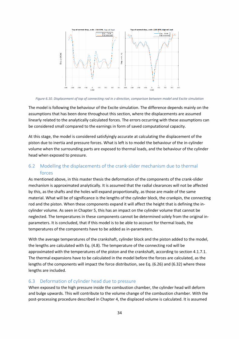
34

Figure 6.10. Displacement of top of connecting rod in z-direction, comparison between model and Excite simulation

The model is following the behaviour of the Excite simulation. The difference depends mainly on the

assumptions that has been done throughout this section, where the displacements are assumed

linearly related to the analytically calculated forces. The errors occurring with these assumptions can

be considered small compared to the earnings in form of saved computational capacity.

At this stage, the model is considered satisfyingly accurate at calculating the displacement of the

piston due to inertia and pressure forces. What is left is to model the behaviour of the in-cylinder

volume when the surrounding parts are exposed to thermal loads, and the behaviour of the cylinder

head when exposed to pressure.

6.2 Modelling the displacements of the crank-slider mechanism due to thermal

forces As mentioned above, in this master thesis the deformation of the components of the crank-slider

mechanism is approximated analytically. It is assumed that the radial clearances will not be affected

by this, as the shafts and the holes will expand proportionally, as those are made of the same

material. What will be of significance is the lengths of the cylinder block, the crankpin, the connecting

rod and the piston. When these components expand it will affect the height that is defining the in-

cylinder volume. As seen in Chapter 5, this has an impact on the cylinder volume that cannot be

neglected. The temperatures in these components cannot be determined solely from the original in-

parameters. It is concluded, that if this model is to be able to account for thermal loads, the

temperatures of the components have to be added as in-parameters.

With the average temperatures of the crankshaft, cylinder block and the piston added to the model,

the lengths are calculated with Eq. (4.8). The temperature of the connecting rod will be

approximated with the temperatures of the piston and the crankshaft, according to section 4.1.7.1.

The thermal expansions have to be calculated in the model before the forces are calculated, as the

lengths of the components will impact the force distribution, see Eq. (6.26) and (6.32) where these

lengths are included.

6.3 Deformation of cylinder head due to pressure When exposed to the high pressure inside the combustion chamber, the cylinder head will deform

and bulge upwards. This will contribute to the volume change of the combustion chamber. With the

post-processing procedure described in Chapter 4, the displaced volume is calculated. It is assumed

35

that the displaced volume due to the deformation of the cylinder head is directly related to the in-

cylinder pressure. The relationship is plotted in Figure 6.11.

Figure 6.11. Volume displacement due to deformation of cylinder head

It is clear in the right plot of Figure 6.11 that the relationship between the displaced volume and the

in-cylinder pressure has linear characteristics. In this master thesis, the displaced volume will be

assumed directly proportional to the in-cylinder pressure, according to:

𝑉𝑑𝑖𝑠𝑝,𝑝𝑟𝑒𝑠𝑠𝑢𝑟𝑒 = 𝐶𝑑𝑖𝑠𝑝,𝑝𝑟𝑒𝑠𝑠𝑢𝑟𝑒 ∗ 𝑃𝑐𝑦𝑙

Where 𝑉𝑑𝑖𝑠𝑝,𝑝𝑟𝑒𝑠𝑠𝑢𝑟𝑒 is the displaced volume due to pressure forces, 𝑃𝑐𝑦𝑙 is the in-cylinder pressure,

and 𝐶𝑑𝑖𝑠𝑝,𝑝𝑟𝑒𝑠𝑠𝑢𝑟𝑒 is a constant that is determined from the data set to best fit the simulated

behaviour.

6.4 Deformation of cylinder head due to thermal forces It was described in Chapter 4 that the FE-simulation calculating the deformations of the cylinder head

is using a heat distribution as load. This heat distribution is calculated from a CFD-simulation. Only

the results of one simulation of a specific operating point has been available during this master

thesis. With the limited amount of data available for the heat distribution and the corresponding

deformation, assumptions have to be made. In the model it will be assumed that the bulging of the

cylinder head is directly proportional to the average temperature in the cylinder liner.

𝑉𝑑𝑖𝑠𝑝,𝑡ℎ𝑒𝑟𝑚𝑎𝑙 = 𝐶𝑑𝑖𝑠𝑝,𝑡ℎ𝑒𝑟𝑚𝑎𝑙 ∗ ∆𝑇

Where 𝑉𝑑𝑖𝑠𝑝,𝑡ℎ𝑒𝑟𝑚𝑎𝑙 is the displaced volume due to thermal forces, ∆𝑇 = 𝑐𝑦𝑙𝑖𝑛𝑑𝑒𝑟 ℎ𝑒𝑎𝑑 − 𝑇𝑟𝑒𝑓 is the

difference in temperature between the mean temperature in the cylinder head and the reference

temperature for which the deformations are zero (room temperature). 𝐶𝑑𝑖𝑠𝑝,𝑡ℎ𝑒𝑟𝑚𝑎𝑙 is a constant

that is determined from the simulated operating point, where temperatures and displacements are

known.

6.5 Deformation of cylinder liner due to thermal load Similarly to the deformation of the cylinder head due to thermal load, the deformation of the

cylinder liner due to thermal load is hard to model accurately with the limited data available. For the

simulated operating point and the corresponding FE-simulation the mean radial strain is known. The

cylinder liner is made of cast iron which has a coefficient of linear thermal expansion of 10.8 10−6𝑚

𝑚∗𝐾.

With the equation of free thermal strain, 𝜖 = 𝛼∆𝑇, the temperature difference corresponding to the

(6.35)

(6.36)

36

strain can be calculated. The temperature difference calculated this way is in accordance with the

temperature from the simulated operating point. In the model of this master thesis, the radial

expansion will be approximated with the equation of free thermal strain.

6.6 Mechanical tolerances The volume of the combustion chamber that is calculated as described in sections 6.1-6.5 will be

considered the expected value of the volume. The mechanical tolerances will define the range of

errors corresponding to the expected value. The mechanical tolerances will be calculated with the

RSS-method with the Bender factor, as described in Chapter 2. In Chapter 2, the tolerances were

calculated when the piston is located at TDC. In the model, the tolerance chain will be calculated as a

function of the crank angle degree. When the crank angle differs from 0 ± 𝑛 ∗ 180° (where 𝑛 is any

integer), the tolerance chain will be altered due to the tilting of the crankpin and connecting rod. The

method here is to project all tolerances onto the z-axis of the cylinder, to find the possible range of

heights the piston can have for a given crank angle.

6.7 The final model After investigating the contribution to the volume change of the different parts, the final model can

be established. Figure 6.12 shows a block scheme of the procedure to calculate the volume.

Figure 6.12. Block scheme of model. Numbers, 6.x refer to the section where respective block is explained.

The first action of the model is to calculate the linear thermal expansions of the connecting rod, the

radius of the crankshaft, the piston and the cylinder block. The mass and pressure forces and

corresponding displacements are calculated with the lengths and the crank angle, RPM and pressure,

the z-coordinate of the piston can be calculated. The volume displacement due to the deformation of

the cylinder head is calculated from the pressure and the temperature of the cylinder head. The

mechanical tolerances are calculated from the crank angle, and the upper and lower limits of the

piston z-coordinate can be determined. Finally, the expected volume, together with upper and lower

limits, are calculated from the length of the cylinder block, the radius of the cylinder liner, the

displaced volume due to deformation of the cylinder head, and the z-coordinate of the piston.

37

7 Results and discussion In this chapter, results obtained with the model will be presented and discussed. The plots will show

a comparison between the volume obtained with the model and the volume obtained from the ideal

piston path. The result will be presented for the operating point of 1200 RPM and high reference

load.

Figure 7.1. Absolute and relative volume difference for a cold engine

Figure 7.2. Absolute and relative volume displacement of a warm engine.

Table 7.1. Approximated temperatures in the warm engine

Component Temperature

Cylinder block 105°𝐶 Cylinder liner 92°𝐶

Crankshaft 108°𝐶 Piston 170°𝐶 Cylinder head 90°𝐶

For the volume difference in the cold engine, Figure 7.1, all temperatures are at reference level, in

other words no thermal expansions are present. For the volume difference in the warm engine,

Figure 7.2, temperatures are approximated according to Table 7.1. The in-cylinder volume that is

calculated with the model differs from the ideal volume, typically within a range of a few percent. It

is interesting to note the difference in characteristics of the volume trace between the cold engine

and the warm. In the cold engine, the major difference between the modelled volume trace and the

ideal volume trace is located at TDCC. When the engine is warm, this volume displacement due to

pressure and inertia forces is counteracted by the expansion of the crank-slider mechanism, and the

largest difference in volume trace is located at TDCGE.

38

The mechanical tolerances can be concluded to have a large impact on the volume trace. At 1200

RPM high reference load and warm engine, it cannot be said with certainty whether the true in-

cylinder volume will be larger or smaller than the ideal volume trace. For the cold engine, the same

conclusion can be made for TDCGE.

To demonstrate the behaviour of the model when load and RPM change, Figure 7.3 and 7.4 show the

volume difference for different loads and engine speeds, for the cold engine. In Figure 7.3, it is clear

that the difference between the modelled volume and the ideal volume increase when the load

increases. In Figure 7.4, the correlation between the engine speed and the volume displacement is

not clear. During the gas exchange strokes (CAD < -180° and CAD > 180°) the displacement is seen to

increase with increased engine speed. However, between TDCc -180° and TDCc +180°, the pressure

forces is dominating and the engine speed is less relevant to the total volume difference.

Figure 7.3 Absolute and relative volume displacement for different loads

Figure 7.4 Absolute and relative volume displacement for different engine speeds

For the cold engine, it is of interest to identify the main causes of deviation from the ideal piston

path. One at the time, each cause for volume deviation will be neglected and the total relative

deviation will be calculated at TDCc and TDCc + 20°. The impacts of each cause for volume deviation

are listed below. TDCc is where the combustion chamber volume is at its smallest and TDCc + 20° is

the point where the total volume deviation is largest.

Table 7.3. Percentage contribution of the different causes for volume deviation for the cold engine. (Values are rounded off)

39

Cause of volume deviation Percent contribution to total volume deviation

at TDCc

Percent contribution to total volume deviation

at TDCc + 20°

Strain of connecting rod 55 % 41 %

Strain of crankpin 15 % 9 %

Bending of crankpin 0 % 7 %

Cylinder head deformation 11 % 8 %

Main bearing clearance 5 % 4 %

Big end bearing clearance 5 % 4 %

Displacement of top of connecting rod in y-dir. 0 % 25 %

The columns in Table 7.3 do not add up to 100 %, this is because of some combination effects from

different deformations that cannot be described by this method. The table will give a general idea of

the different contributions. At both TDCc and TDCc + 20°, the largest cause of volume deviation is the

strain of the connecting rod. This is especially of interest as the connecting rod in the Excite model is

considered a bar element. To increase the accuracy of the model, the behaviour of the connecting

rod needs to be further analysed. As suggestion of how to do this, is to simply apply forces to a FE-

model of the connecting rod, and determine the stress-strain relationship.

A large contributor to the total volume deviation at TDCc + 20° is the displacement of the top of the

connecting rod in y-direction. It is mentioned before that this displacement is unreasonable large in

the Excite simulation and it would be advisable to investigate this further to improve the accuracy of

the model.

7.1 Error analysis The model is approximating the volume based on linearized relations. The advantage of this is that

the model never iterates, and never solves any non-linear equations and can therefor calculate the

volume in real time. The disadvantage is of course the loss of accuracy compared with a FE-solver or

MBS program. The error that occurs when the model is approximating the position of the piston in z-

direction for a cold engine can be quantified by comparing with the Excite simulation, see Figure 7.5.

Figure 7.5. Relative error between model and Excite simulation relative to the ideal volume trace

Figure 7.5 shows plots with the relative volume difference between the model and the Excite

simulation. The relative errors are, as expected, largest around TDCC and TDCGE (where the total

volume is smallest) with values < 1 % of the cylinder total volume. The error tends to be larger with

larger load and higher RPM.

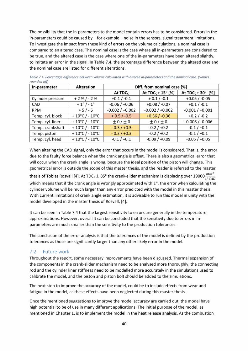
40

The possibility that the in-parameters to the model contain errors has to be considered. Errors in the

in-parameters could be caused by – for example – noise in the sensors, signal treatment limitations.

To investigate the impact from these kind of errors on the volume calculations, a nominal case is

compared to an altered case. The nominal case is the case where all in-parameters are considered to

be true, and the altered case is the case where one of the in-parameters have been altered slightly,

to imitate an error in the signal. In Table 7.4, the percentage difference between the altered case and

the nominal case are listed for different alterations.

Table 7.4. Percentage difference between volume calculated with altered in-parameters and the nominal case. (Values rounded off)

In-parameter Alteration Diff. from nominal case [%]

At TDCC At TDCC + 15° [%] At TDCC + 30° [%]

Cylinder pressure + 2 % / - 2 % +0.1 / -0.1 + 0.1 / -0.1 +0.05 / -0.05

CAD + 1° / - 1° -0.06 / +0.06 +0.08 / -0.07 +0.1 / -0.1

RPM + 5 / - 5 -0.002 / +0.002 -0.002 / +0.002 -0.001 / +0.001

Temp. cyl. block + 10°C / - 10°C + 0.5 / -0.5 +0.36 / -0.36 +0.2 / -0.2

Temp. cyl. liner + 10°C / - 10°C ± 0 / ± 0 ± 0 / ± 0 +0.006 / -0.006

Temp. crankshaft + 10°C / - 10°C - 0.3 / +0.3 -0.2 / +0.2 -0.1 / +0.1

Temp. piston + 10°C / - 10°C - 0.3 / +0.3 -0.2 / +0.2 -0.1 / +0.1

Temp. cyl. head + 10°C / - 10°C -0.1 / +0.1 -0.09 / +0.09 -0.05 / +0.05

When altering the CAD signal, only the error that occurs in the model is considered. That is, the error

due to the faulty force balance when the crank angle is offset. There is also a geometrical error that

will occur when the crank angle is wrong, because the ideal position of the piston will change. This

geometrical error is outside the scope of this master thesis, and the reader is referred to the master

thesis of Tobias Rosvall [4]. At TDCc ± 85° the crank-slider mechanism is displacing over 19000𝑚𝑚3

1° 𝐶𝐴𝐷,

which means that if the crank angle is wrongly approximated with 1°, the error when calculating the

cylinder volume will be much larger than any error predicted with the model in this master thesis.

With current limitations of crank angle estimation, it is advisable to run this model in unity with the

model developed in the master thesis of Rosvall, [4].

It can be seen in Table 7.4 that the largest sensitivity to errors are generally in the temperature

approximations. However, overall it can be concluded that the sensitivity due to errors in in-

parameters are much smaller than the sensitivity to the production tolerances.

The conclusion of the error analysis is that the tolerances of the model is defined by the production

tolerances as those are significantly larger than any other likely error in the model.

7.2 Future work Throughout the report, some necessary improvements have been discussed. Thermal expansion of

the components in the crank-slider mechanism need to be analysed more thoroughly, the connecting

rod and the cylinder liner stiffness need to be modelled more accurately in the simulations used to

calibrate the model, and the piston and piston bolt should be added to the simulations.

The next step to improve the accuracy of the model, could be to include effects from wear and

fatigue in the model, as these effects have been neglected during this master thesis.

Once the mentioned suggestions to improve the model accuracy are carried out, the model have

high potential to be of use in many different applications. The initial purpose of the model, as

mentioned in Chapter 1, is to implement the model in the heat release analysis. As the combustion

41

chamber volume, as well as the volume derivative is included in the heat release equation, the

accuracy of the heat release analysis could be improved with the model.

The model is not restricted to work only for the heat release analysis, all models that describes the

combustion and/or the chemical process in the combustion chamber and include the in-cylinder

volume have the potential to be more accurate if this model is implemented.

42

8 Conclusions In this brief chapter, the conclusions made from this master thesis will be listed.

1. With the developed model, the combustion chamber volume can be approximated with

linearized relations, based on crank angle degree, in-cylinder pressure and temperatures of

certain components.

2. The combustion chamber volume approximated with the model differs from the ideal

combustion chamber volume typically within a range of a few percent. The relative volume

difference is for all cases largest at TDC. The volume difference tends to decrease as the

engine becomes warmer, as the thermal expansions counteract the deformations due to

inertia and pressure forces.

3. For the cold engine, the deformation of the connecting rod is the largest contribution to the

total volume difference. The displacement of the connecting rod in y-direction is also a large

contribution to the total volume difference.

4. Errors in the volume calculation caused by errors in the in-parameters and errors between

the model and the simulations are small compared to the mechanical tolerances. The

production tolerances will define the tolerance of the model.

5. To increase the accuracy of the model, the thermal expansions, the strain of the connecting

rod and the stiffness of the cylinder liner need to be analysed more thoroughly. Also the

piston bolt and the piston should be added to the model as flexible bodies.

6. The production tolerances of the length of the cylinder block and the length of the crankpin

are together corresponding for over 65 % of the assembly tolerance.

7. The model developed in this master thesis has potential to increase the accuracy of the heat

release analysis model and other models that describes the combustion and/or the chemical

process in the combustion chamber and include the in-cylinder volume.

43

9 Bibliography

[1] C. R. Ferguson and A. T. Kirkpatrick, Internal Combustion Engines: applied thermodynamics -

2nd. ed., New Jersey: John Wiley & Sons, Inc., 2001.

[2] U. Aronsson et al., “Impact of Mechanical Deformation due to Pressure, Mass, and Thermal

Forces on the In-Cylinder Volume Trace in Optical Engines of Bowditch Design”, Lund

University, Lund, Sweden, SAE Tech. Paper 2011-26-0082, 2011, doi:10.4271/2012-01-2011-26-

0082.

[3] U. Aronsson et al., “Analysis of Errors in Heat Release Calculations Due to Distortion of the In-

Cylinder Volume Trace from Mechanical Deformation in Optical Diesel Engines,” Lund

University, Lund, Sweden, SAE Tech. Paper 2012-01-1604, 2012, doi:10.4271/2012-01-1604.

[4] T. Rosvall, “Master Thesis: Design of Virtual Crank Angle Sensor based on Torque Estimation,”

Kungliga Tekniska Högskolan, Stockholm, 2015.

[5] R. R. Malagi, et al., “Finite Element Study on Piston Assembly Dynamics in Multicylinder Internal

Combustion Engine,” Gogte Inst. of Technology, Karnataka, India, SAE Tech. Paper 2011-01-

1075, 2011, doi:10.4271/2011-01-1075.

[6] C. Hebert and W. Webster, “Cylinder Head Gasket Simulation in Finite Element Analysis” in Int.

Congr. and Expo., Detroit, MI, USA, SAE Tech. Paper 980843, 1998, doi:10.4271/980843.

[7] T. R. Meyer and R. A. White, “The Effects of Cylinder Head Deformation and Asymmetry on

Exhaust Valve Thermo-Mechanical Stresses”, in Int. Congr. and Expo., Detroit, MI, USA, SAE

Tech. Paper 981034, 1998, doi:10.4271/981034.

[8] E. Oanta and D. Taraza, ” Experimental Investigation of the Strains and Stresses in the Cylinder

Block of a Marine Diesel Engine” in SAE 2000 World Congr., Detroit, MI, USA, SAE Tech. Paper

2000-01-0520, 2000, doi:10.4271/2000-01-0520.

[9] K. W. Chase, “BASIC TOOLS FOR TOLERANCE ANALYSIS OF MECHANICAL ASSEMBLIES,” in

MANUFACTURING ENGINEERING HANDBOOK, New York, McGraw-Hill, 2004, pp. 7.1-7.12.

[10] F. Scholz, “Tolerance Stack Analysis Methods,” Boeing Information & Support Services, Seattle,

1995.

[11] MSC Software Corp., Dynamic Analysis User's Guide, Newport Beach, CA, USA: MSC Software

Corp., 2014.

[12] AVL LIST GmbH, Theory AVL EXCITE POWER UNIT VERSION 2014, Graz, Austria: AVL LIST GmbH,

2014.

[13] U. Mohammed , et al., “Analysis of Parameters Affecting Liner Bore Distortion in DI Diesel

Engines,” Kirloskar Oil Engines Ltd., Khadki, India, SAE Tech. Paper 2015-26-0178, 2015,

doi:10.4271/2015-26-0178.

44

[14] F. Koch, et al., “Cylinder Liner Deformation Analysis – Measurements and Calculations,” in Int.

Congr. and Expo., Detroit, MI, USA, SAE Tech. Paper 980567, 1998, doi:10.4271/980567.

[15] B. Johansson, Förbränningsmotorer del 2, Lund, Sweden: Avdelningen för Förbränningsmotorer

Lunds Tekniska Högskola, 2004.

[16] N. Noda, R. B. Hetnarski and Y. Tanigawa, “Free Thermal Expansion and Free Thermal Strain,” in

Thermal Stresses - Second Edition, New York, Taylor & Francis, 2003, pp. 4-5.

[17] Springer Viewg, Pistons and engine testing, 2nd Edition, Stuttgart, Germany: MAHLE GmbH,

2016.

[18] C. Ljung, N. Saabye Ottosen and M. Ristinmaa, Introduktion till hållfasthetslära, Enaxliga

tillstånd, Lund, Sweden: Studentlitteratur, 2007.