CYCLONE GLOBAL NAVIGATION SATELLITE...

CYCLONE GLOBAL NAVIGATION SATELLITE SYSTEM (CYGNSS)

End-to-End Simulator Technical Memo

UM Doc. No. 148-0123 SwRI Doc. No. N/A Revision 0 Date 2 January 2014 Contract NNL13AQ00C

CYCLONE GLOBAL NAVIGATION SATELLITE SYSTEM (CYGNSS)

End-to-End Simulator Technical

Memo UM Doc. No. 148-0123 SwRI Doc. No. N/A Revision 0 Date 2 Jan 2014 Contract NNL13AQ00C

Prepared by: Andrew O’Brien, Ohio State University Date: 1/2/14 Approved by: Email approval on file Date: 1/20/2014 Chris Ruf, CYGNSS Principal Investigator Approved by: Email approval on file Date: 1/20/2014 John Scherrer, CYGNSS Project Manager Approved by: Email approval on file Date: 1/20/2014 Randy Rose, CYGNSS Project Systems Engineer Released by: Email approval on file Date: 1/20/2014 Damen Provost, CYGNSS UM Project Manager

3

REVISION NOTICE

Document Revision History

Revision Date Changes

Initial Release 2 January 2014 n/a

CYGNSS End-to-End Simulator (E2ES) Technical Memo

Contents

1 Introduction 41.1 Process Overview . . . . . . . . . . . . . . . . . . . . . . . . . . . . . . . . . . . . . . . . . . . 4

2 Transmitter and Receiver Geometry 5

3 Surface Grid 63.1 Surface Geometry . . . . . . . . . . . . . . . . . . . . . . . . . . . . . . . . . . . . . . . . . . . 7

3.1.1 Geometric Parameters over the Surface . . . . . . . . . . . . . . . . . . . . . . . . . . 73.1.2 Latitude, Longitude and the ENU Frame . . . . . . . . . . . . . . . . . . . . . . . . . 9

3.2 Surface Gridding . . . . . . . . . . . . . . . . . . . . . . . . . . . . . . . . . . . . . . . . . . . 103.3 Physical Fields . . . . . . . . . . . . . . . . . . . . . . . . . . . . . . . . . . . . . . . . . . . . 11

3.3.1 Wind Field . . . . . . . . . . . . . . . . . . . . . . . . . . . . . . . . . . . . . . . . . . 113.3.2 Minimum Wind Speed . . . . . . . . . . . . . . . . . . . . . . . . . . . . . . . . . . . . 123.3.3 Rain Rate, Freezing Height and Permitivity . . . . . . . . . . . . . . . . . . . . . . . . 12

4 Scattering Model 124.1 Ocean Surface Model . . . . . . . . . . . . . . . . . . . . . . . . . . . . . . . . . . . . . . . . . 124.2 Bistatic RCS . . . . . . . . . . . . . . . . . . . . . . . . . . . . . . . . . . . . . . . . . . . . . 134.3 Rain Attenuation . . . . . . . . . . . . . . . . . . . . . . . . . . . . . . . . . . . . . . . . . . . 144.4 Antenna Patterns . . . . . . . . . . . . . . . . . . . . . . . . . . . . . . . . . . . . . . . . . . . 14

5 Delay-Doppler Map (DDM) Calculation 155.1 Reflected Signal . . . . . . . . . . . . . . . . . . . . . . . . . . . . . . . . . . . . . . . . . . . . 155.2 Speckle . . . . . . . . . . . . . . . . . . . . . . . . . . . . . . . . . . . . . . . . . . . . . . . . 165.3 DDM Generation in the E2ES . . . . . . . . . . . . . . . . . . . . . . . . . . . . . . . . . . . . 17

6 Using the E2ES 186.1 Compilation . . . . . . . . . . . . . . . . . . . . . . . . . . . . . . . . . . . . . . . . . . . . . . 186.2 Running the E2ES . . . . . . . . . . . . . . . . . . . . . . . . . . . . . . . . . . . . . . . . . . 196.3 Configuration File . . . . . . . . . . . . . . . . . . . . . . . . . . . . . . . . . . . . . . . . . . 196.4 File Formats . . . . . . . . . . . . . . . . . . . . . . . . . . . . . . . . . . . . . . . . . . . . . 22

3


1 Introduction

This document describes the technical methodology behind the implementation of the CYGNSS End-to-EndSimulator (E2ES). The E2ES is a detailed software simulator of the CYGNSS mission that is currently underdevelopment. It heavily leverages the experience and expertise of those members of the CYGNSS ScienceTeam who pioneered the theoretical conception and experimental development of GNSS remote sensing overthe past 10+ years. Ultimately, the simulator will model all critical steps of the wind speed retrieval process,including

• Dynamic orbit propagators for GPS and CYGNSS constellations

• Signal generation by GPS transmitter satellites

• Propagation to the specular reflection point (including rain attenuation) on the Earth surface

• Bi-static forward scattering from the wind driven, roughened ocean surface

• Receive antenna gain pattern projected onto the Earth surface

• Link budget for received signal strength

• Fading and thermal noise statistics of received signal

• Accurate and precise delay doppler map data product

1.1 Process Overview

The CYGNSS E2ES is organized into a set of fundamental blocks that are executed sequentially. Figure1 shows an overview of the simulator process flow. The E2ES process starts with an initialization phase.A configuration file is provided by the user and used to allocate memory for data structures, load inputfiles and set a number of user-definable parameters. The contents of this configuration file are discussed inSection 6.

After initialization, the transmitter and receiver orbit information is input by the user. The orbit in-formation is in the form of position and velocity in ECEF coordinates. For a simple simulation, a singletransmitter and receiver can be specified manually in the configuration file. For a realistic orbit simulation,a sequence of positions and velocities can be input from a file for multiple transmitters and receivers. Basedon the WGS-84 model of the Earth, the E2ES solves for the point on the Earth where the reflection ofthe transmitted signal takes place (i.e. the specular point) using an efficient iterative approach. Once thespecular point is found, the receiver and transmitter geometry are rotated into a reference frame based onthe specular location in order to form the fundamental bistatic radar geometry around this point.

Next, the Earth’s surface around the specular location is discretized into a grid. The curvature of theEarth is accurately accounted for in this grid using a spherical Earth approximation around the specularlocation. The discretized surface is then composed of a dense grid of patches, each one having its owngeometry with respect to the transmitter and receiver.

Once the grid is constructed, the geometric parameters of each patch are evaluated. These parametersinclude the range, delay, Doppler and scattering angle. The relative angle of each patch to the transmitterand receiver antennas are calculated, and the transmitter and receiver antenna gain are found for eachlocation on the surface. At this point, the physical parameters of the surface are also loaded. These includethe wind speed and direction, rain rate, freezing height, and surface permitivity. The wind field are used tocalculate the expected mean square slope (MSS) of the ocean surface. This, in turn, is used to calculate theradar cross section of the surface patch and ultimately the total scattered power.

Given the expected scattered power of each surface patch, the E2ES uses this information to accuratelyrepresent the effect of speckle on the scattered signal received by CYGNSS. The actual scattered field ofthe surface patch is initialized as a random variable with a random initial phase. However, the phase of thescattered field also depends on geometry, so as the satellites move in time, the phase will advance for each

4


Figure 1: Overview of E2ES Process

patch differently. This results in random fading noise in the reflected signal and accurately represents thecorrect statistical properties observed in actual space-based GNSS-R measurements.

The scattered field is used to form a delay Doppler map (DDM). Thermal noise is added to the DDM, andthe ambiguity function of the GPS C/A code signal is convolved with the noisy DDM in order to accuratelyaccount for the bin-to-bin correlation. This represents a complex DDM produced after a 1 millisecondcoherent integration. The process is repeated 1000 times and non-coherently averaged to produce a single1-second DDM product. The DDM is then down sampled to match the resolution of the actual CYGNSSmeasurements.

2 Transmitter and Receiver Geometry

The E2ES considers a single transmitter and receiver at a time. The input to the E2ES is the position andvelocities of the transmitter and receiver in Earth-centered Earth-fixed (ECEF) coordinates,

�rR : receiver position (1)�rT : transmitter position (2)�vR : receiver velocity (3)�vT : transmitter velocity (4)

The specular reflection point is assumed to lie on the surface of the WGS-84 Ellipsoid and is calculatedusing the iterative method described in [5], with open source code provided in [6]. The resulting calculation

5


yields the specular point position �rP in ECEF coordinates,

�rP : specular point position (5)

After the specular point has been found, a specular frame coordinate system is defined. In the specularframe, depicted in Figure 2, the z-axis is normal to the Earth’s surface at the specular point, the x-axis isalong the direction from the transmitter to the receiver, and the y-axis completes the right-hand system.The rotation matrix between the ECEF frame and specular frame RSPEC

ECEF is given by

RSPECECEF =

[x y z

]T (6)

z =�rS

‖�rS‖ (7)

x =�rTR − �rTR · x‖�rTR − �rTR · x‖ (8)

y = z × x (9)

where �rTR is the relative position between the transmitter and receiver,

�rTR = �rR − �rT . (10)

Figure 2: Definition of specular reference frame.

3 Surface Grid

Having solved for the specular point, the E2ES next discretizes the Earth’s surface around this point. Thecurvature of the Earth is accurately accounted for in this grid using a spherical Earth approximation aroundthe specular location. First, we will describe the geometry of the continuous surface. Then, the surfacewill be discretized to form dense grid of patches, each one having its own geometry with respect to thetransmitter and receiver.

6


3.1 Surface Geometry

Currently, the E2ES approximates the Earth’s surface as the surface of a sphere with a radius equal to theradius of the Earth at the specular point re

re = ‖�rP ‖ . (11)

The locations of surface points rs in the specular frame are parameterized with the traditional sphericalcoordinates (θ, φ)

�rS(θ, φ) =

⎡⎣re sin θ cos φ

re sin θ sin φre cos θ

⎤⎦ (12)

where the specular point corresponds to (θ, φ) = (0, 0). A local surface frame is defined at each (θ, φ)location as

n(θ, φ) =

⎡⎣sin θ cos φ

sin θ sin φcos θ

⎤⎦ , (13)

θ(θ, φ) =

⎡⎣cos θ cos φ

cos θ sin φ− sin θ

⎤⎦ , (14)

φ(θ, φ) =

⎡⎣− sin φ

cos φ0

⎤⎦ (15)

where n is normal to the surface and θ and φ are tangential to it. Together they form the local rotationmatrix between the specular frame and the surface frame

RSURFSPEC(θ, φ) =

[n(θ, φ) θ(θ, φ) φ(θ, φ)

]T

(16)

The differential area over the surface is given by

dA(θ, φ) = r2e sin θ dθ dφ . (17)

3.1.1 Geometric Parameters over the Surface

Each point (θ, φ) on the surface forms its own bistatic radar geometry with the transmitter and receiver.The vectors pointing from a location on the surface to the receiver or transmitter in the specular frame is

�rSR(θ, φ) = RSPECECEF�rR − �rS(θ, φ) (18)

�rST (θ, φ) = RSPECECEF�rT − �rS(θ, φ) (19)

where the path lengths are

RSR(θ, φ) = ‖�rSR(θ, φ)‖ (20)RST (θ, φ) = ‖�rST (θ, φ)‖ (21)

and the unit vectors pointing from the surface to the receiver or transmitter in the specular frame are

�uSR(θ, φ) =�rSR(θ, φ)RSR(θ, φ)

(22)

�uST (θ, φ) =�rSR(θ, φ)RST (θ, φ)

(23)

7


Figure 3: Parameterization of the Earth’s surface around the specular point

The line-of-sight velocities to the transmitter and receiver wrt. a location on the surface are

vSR(θ, φ) = �uSR(θ, φ) · RSPECECEF�vR (24)

vST (θ, φ) = �uST (θ, φ) · RSPECECEF�vT (25)

The delay τD and Doppler fD over the surface is

τD(θ, φ) =1c

(RSR(θ, φ) + RSR(θ, φ)

)(26)

fD(θ, φ) = −fL1

c

(vSR(θ, φ) + vST (θ, φ)

)(27)

where fL1 is the GPS L1 center frequency. We are primarily interested in the delay and Doppler relative tothe specular point at (θ, φ) = (0, 0),

τ ′D(θ, φ) = τD(θ, φ) − τD(0, 0) (28)

f ′D(θ, φ) = f ′

D(θ, φ) − f ′D(0, 0) (29)

The incident angle θi between the surface location and either the transmitter or receiver are

θi,R(θ, φ) = cos−1 (n(θ, φ) · �uSR(θ, φ)) (30)θi,T (θ, φ) = cos−1 (n(θ, φ) · �uST (θ, φ)) (31)

and the scattering angle θs is

θs(θ, φ) =12cos−1

(− �uST (θ, φ) · �uSR(θ, φ)

)(32)

The scattering vector �q in the local surface coordinate system is defined as

�q(θ, φ) =2πfL1

cRSURF

SPEC(θ, φ)(�uSR(θ, φ) + �uST (θ, φ)

)(33)

8


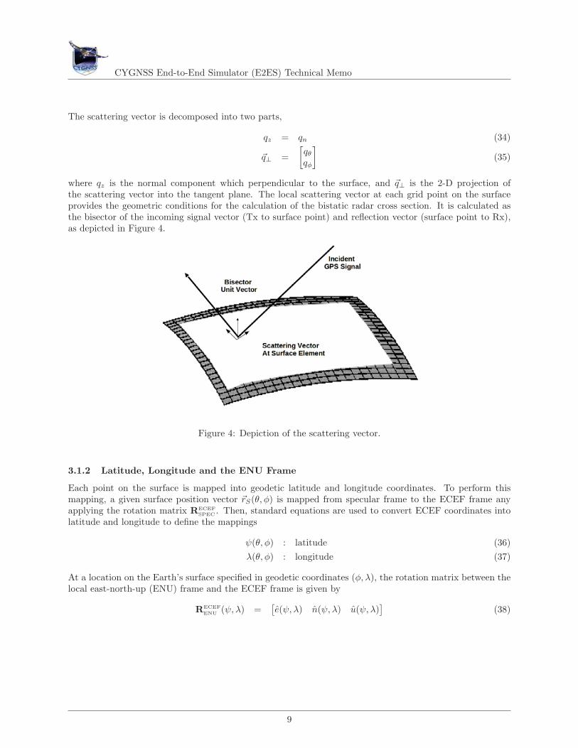
The scattering vector is decomposed into two parts,

qz = qn (34)

�q⊥ =[qθ

qφ

](35)

where qz is the normal component which perpendicular to the surface, and �q⊥ is the 2-D projection ofthe scattering vector into the tangent plane. The local scattering vector at each grid point on the surfaceprovides the geometric conditions for the calculation of the bistatic radar cross section. It is calculated asthe bisector of the incoming signal vector (Tx to surface point) and reflection vector (surface point to Rx),as depicted in Figure 4.

Figure 4: Depiction of the scattering vector.

3.1.2 Latitude, Longitude and the ENU Frame

Each point on the surface is mapped into geodetic latitude and longitude coordinates. To perform thismapping, a given surface position vector �rS(θ, φ) is mapped from specular frame to the ECEF frame anyapplying the rotation matrix RECEF

SPEC . Then, standard equations are used to convert ECEF coordinates intolatitude and longitude to define the mappings

ψ(θ, φ) : latitude (36)λ(θ, φ) : longitude (37)

At a location on the Earth’s surface specified in geodetic coordinates (φ, λ), the rotation matrix between thelocal east-north-up (ENU) frame and the ECEF frame is given by

RECEFENU (ψ, λ) =

[e(ψ, λ) n(ψ, λ) u(ψ, λ)

](38)

9


where

e(ψ, λ) =

⎡⎣− sin λ

cos λ0

⎤⎦ (39)

n(ψ, λ) =

⎡⎣− cos λ sin ψ− sin λ sin ψ

cos ψ

⎤⎦ (40)

u(ψ, λ) =

⎡⎣cos λ cos ψ

sin λ cos ψsin ψ

⎤⎦ (41)

Using (38), we can assemble the rotation matrix between the ENU and surface frames

RSURFENU (θ, φ) = RSURF

SPEC(θ, φ) RSPECECEF RECEF

ENU

(ψ(θ, φ), λ(θ, φ)

)(42)

This transformation will be primarily utilized to convert 2-D surface vector fields from east-north coordinatesinto surface coordinates. In this case, we define the restriction matrix

P =[1 0 00 1 0

](43)

so that the 2-D transformation is represented as

TSURFENU (θ, φ) = P RSURF

ENU (θ, φ) PT (44)

Since the surface is a spherical Earth approximation of the true WGS84 ellipsoid, the normal vector n andu will only be the same at the specular point. (44) represents the projection of the tangential vector fromthe ellipsoidal surface to the spherical surface.

3.2 Surface Gridding

In the E2ES, the surface is discretized. The discretization is determined by three user specified parameters:

d : minimum surface resolution (meters) (45)Nθ : number of grid points in the θ direction (46)Nφ : number of grid points in the φ direction (47)

These parameters define a discrete set of angles {θi} and {φj},

θi = (i −⌊Nθ

2

⌋)Δθ for i = 1 . . . Nθ (48)

φj = (j −⌊Nφ

2

⌋)Δφ for j = 1 . . . Nφ (49)

where the angular increments Δθ and Δφ determined by the specified surface resolution

Δθ = Δφ =d

re. (50)

We refer to this set of discrete angles as the surface grid. Note that this definition ensures the specularpoint (θ, φ) = (0, 0) is always included in the set of angles.

In this way, the surface is discretized into patches, and the set of angles correspond to the center of eachsurface patch. Figure ?? shows what this grid looks like. The location of each patch in the specular frameis denoted

�s[i, j] = �s(θi, φj), (51)

10


and the area ΔA of the each patch is

ΔA[i, j] = r2e sin (θi) Δθ Δφ (52)

Note that the surface resolution only determines the maximum patch size (i.e. d2), and patches away fromspecular will be slightly smaller. Each patch is considered flat with normal and tangential vectors given byits surface frame,

RSURFSPEC[i, j] = RSURF

SPEC(θi, φj), (53)

Figure 5: Surface grid.

3.3 Physical Fields

Having constructed a surface grid, the next step is to associate each location with physical properties, such assurface wind speed, wind direction, rain rate, freezing height, and permitivity. The E2ES configuration filespecifies a file which contains this physical information over some region of the Earth that is to be utilized.Note that all the input fields are defined in some suitable spatial resolution in geodetic coordinates andlinearly interpolated when specified over the surface grid.

3.3.1 Wind Field

The input wind fields are specified by their U10 and V10 components, which correspond to the eastwardand northward components at 10 meter height above the ocean surface, respectively. The components aredenoted wU10(ψ, λ) and wU10(ψ, λ). The wind vector �w in geodetic coordinates in the ENU frame is formedas

�w(ψ, λ) = wU10(ψ, λ)e(ψ, λ) + wV 10(ψ, λ)n(ψ, λ) (54)

and is converted into surface coordinates in the surface frame

�w(θ, φ) = TSURFENU (θ, φ)�w

(ψ(θ, φ), λ(θ, φ)

)(55)

11


Once it is in the surface frame, it can be decomposed into wind speed vw and wind direction angle φ0 formedwrt. the φ-axis

vw(θ, φ) = ‖�w(θ, φ)‖ (56)

φw(θ, φ) = cos−1( �w(θ, φ) · φ(θ, φ)

vw(θ, φ)

)(57)

The wind speed and wind direction angle fields over the surface are then directly used to find the surfaceMSS as described in a later section of this document.

3.3.2 Minimum Wind Speed

The E2ES supports a constraint that the wind field have at least a particular minimum wind speed. Thisconstraint can be enforced globally or over a particular region. The region is a user defined circle specifiedby the latitude and longitude of the center and a radial distance. These parameters can be defined as atime-varying sequence and are input into the E2ES in the form of a binary file. A minimum wind speedspecified in this way is a simple means of accounting for swell in the eye of a tropical cyclone. In the eye,the wind speed is very low, but swell contributes to the MSS. Instead of specifying swell, a minimum windspeed can be used to produce similar scattering behavior.

3.3.3 Rain Rate, Freezing Height and Permitivity

The rain rate R(ψ, λ) and freezing height h(ψ, λ) fields are also loaded into the E2ES. These are used tocalculate the rain attenuation factor. Again, they are input in geodetic coordinates and converted intosurface coordinates

R(θ, φ) = R(ψ(θ, φ), λ(θ, φ)

)(58)

h(θ, φ) = h(ψ(θ, φ), λ(θ, φ)

)(59)

The complex dielectric constant of the medium ε is used when solving for the reflection coefficient of thesurface. Although the E2ES supports a spatially varying dielectric constant, it currently assumes a simplydielectric constant of sea water

ε(θ, φ) = 74.62 + i51.92. (60)

4 Scattering Model

4.1 Ocean Surface Model

Each patch on the gridded ocean surface is characterized by its own probability density function of sur-face slopes P (�s) pertinent for reflection. For our numerical simulations, we utilize Gaussian statistics ofanisotropic slopes

P (�s) =1

2πσsxσsy

√1 − b2

x,y

exp

(− 1

2(1 − b2x,y)

(s2

x

σ2sx

− 2bx,ysxsy

σsxσsy

+s2

y

σ2sy

))(61)

where �s is the slope vector in surface x-y coordinates.

12


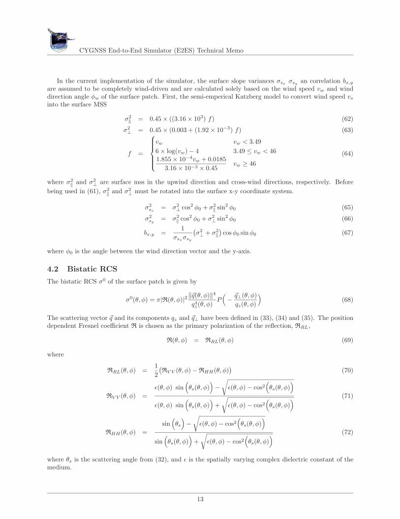
In the current implementation of the simulator, the surface slope variances σsx σsy an correlation bx,y

are assumed to be completely wind-driven and are calculated solely based on the wind speed vw and winddirection angle φw of the surface patch. First, the semi-emperical Katzberg model to convert wind speed vs

into the surface MSS

σ2‖ = 0.45 × ((3.16 × 103) f) (62)

σ2⊥ = 0.45 × (0.003 + (1.92 × 10−3) f) (63)

f =

⎧⎪⎪⎪⎨⎪⎪⎪⎩

vw vw < 3.496 × log(vw) − 4 3.49 ≤ vw < 461.855 × 10−4vw + 0.0185

3.16 × 10−3 × 0.45vw ≥ 46

(64)

where σ2‖ and σ2

⊥ are surface mss in the upwind direction and cross-wind directions, respectively. Beforebeing used in (61), σ2

‖ and σ2⊥ must be rotated into the surface x-y coordinate system.

σ2sx

= σ2⊥ cos2 φ0 + σ2

‖ sin2 φ0 (65)

σ2sy

= σ2‖ cos2 φ0 + σ2

⊥ sin2 φ0 (66)

bx,y =1

σsxσsy

(σ2⊥ + σ2

‖)cos φ0 sin φ0 (67)

where φ0 is the angle between the wind direction vector and the y-axis.

4.2 Bistatic RCS

The bistatic RCS σ0 of the surface patch is given by

σ0(θ, φ) = π|R(θ, φ)|2 ‖�q(θ, φ)‖4

q4z(θ, φ)

P(− �q⊥(θ, φ)

qz(θ, φ)

)(68)

The scattering vector �q and its components qz and �q⊥ have been defined in (33), (34) and (35). The positiondependent Fresnel coefficient R is chosen as the primary polarization of the reflection, RRL,

R(θ, φ) = RRL(θ, φ) (69)

where

RRL(θ, φ) =12(RV V (θ, φ) − RHH(θ, φ)

)(70)

RV V (θ, φ) =ε(θ, φ) sin

(θs(θ, φ)

)−

√ε(θ, φ) − cos2

(θs(θ, φ)

)

ε(θ, φ) sin(θs(θ, φ)

)+


(θs(θ, φ)

) (71)

RHH(θ, φ) =sin

(θs

)−


(θs(θ, φ)

)

sin(θs(θ, φ)

)+


(θs(θ, φ)

) (72)

where θs is the scattering angle from (32), and ε is the spatially varying complex dielectric constant of themedium.

13


4.3 Rain Attenuation

CYGNSS uses the GPS L1 frequency (1575 MHz ) which exhibits negligible rain attenuation, even underheavy precipitating conditions. Nonetheless, the E2ES accurately accounts for rain attenuation Grain usingthe formula

Grain(θ, φ) = exp(− α(θ, φ) h(θ, φ)

(csc θi,T (θ, φ) + csc θi,T (θ, φ)

))(73)

where h is the freezing height in km and α is the specific attenuation (Np/km). θi,T and θi,R are the elevationangles to the transmitter and receiver, respectively, given by equations (30) and (30). Note that all of theseparameters vary over the surface, so the E2ES is accurately accounting for the spatial variations in the rainfield. For simplicity, the current rain attenuation model assumes that the rain rate is constant from thesurface up to freezing height.

The specific attenuation is obtained from the ITU R838-3 [11] model,

α(θ, φ) = aRb(θ, φ) (74)a = 24.312 × 10−5 (75)b = 0.9567 (76)

where R is the rain rate (mm/hr) and a and b are the model coefficients for circular polarization at the GPSL1 frequency, whose values have been developed from curve-fitting to power-law coefficients derived fromscattering calculations.

4.4 Antenna Patterns

The antenna gain patterns for the transmitter and receiver are loaded from files specified in the configurationfile input to the E2ES. In these files, the antenna patterns are specified in azimuth and elevation angles withrespect to the satellite vehicle frame. Based on the satellite orbits, the E2ES creates a gain pattern of eachantenna over the surface grid.

A separate orbit frame is defined for both the transmitter and receiver satellites. In this frame the x-axispoints in the direction of the satellite velocity vector, the z-axis points down toward the center of the Earth,and the y-axis completes a right-hand system. The rotation matrix between the specular frame and receiverorbit frame is given by

RORB,RxSPEC =

[x y z

]T (77)

x =�vR

‖�vR‖ (78)

z = − �rR − �rR · x‖�rR − �rR · x‖ (79)

y = z × x (80)

and similarly for the transmitter. A satellite vehicle body frame is defined, and the vehicle could have someattitude within the orbit frame. The rotation matrix between the satellite orbit and vehicle frames are userspecified parameters,

RVEH,RORB,R : receiver orbit to vehicle frame (81)

RVEH,TORB,T : transmitter orbit to vehicle frame (82)

The vectors pointing from the satellite to each location on the surface are given by

�rRS(θ, φ) = �rS(θ, φ) − RSPECECEF�rR − (83)

�rTS(θ, φ) = �rS(θ, φ) − RSPECECEF�rT (84)

14


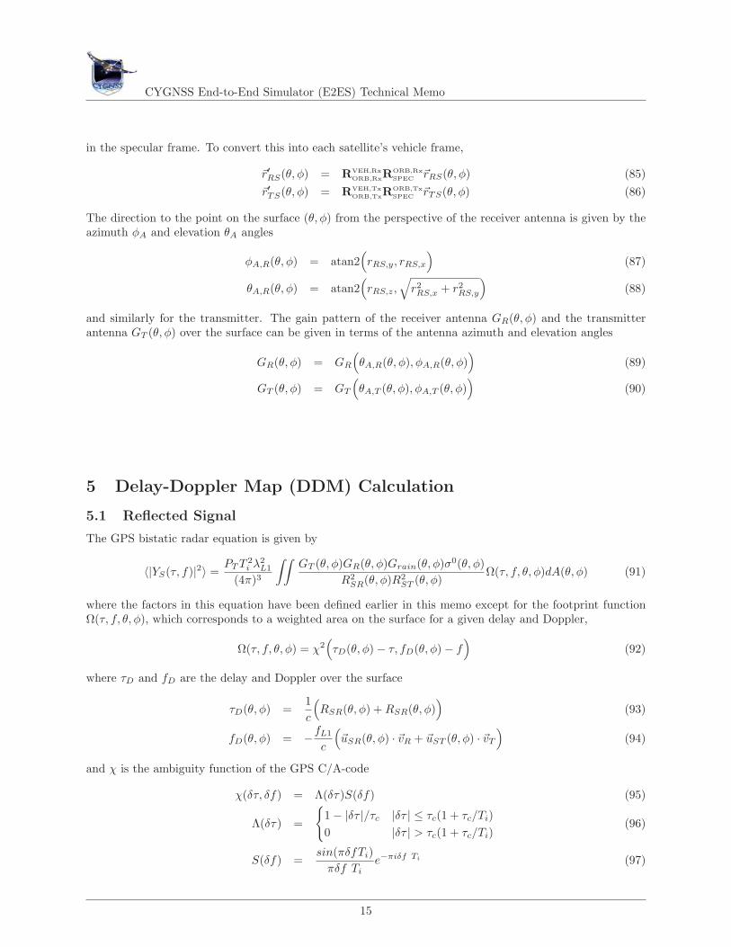
in the specular frame. To convert this into each satellite’s vehicle frame,

�r′RS(θ, φ) = RVEH,RxORB,RxR

ORB,RxSPEC �rRS(θ, φ) (85)

�r′TS(θ, φ) = RVEH,TxORB,TxR

ORB,TxSPEC �rTS(θ, φ) (86)

The direction to the point on the surface (θ, φ) from the perspective of the receiver antenna is given by theazimuth φA and elevation θA angles

φA,R(θ, φ) = atan2(rRS,y, rRS,x

)(87)

θA,R(θ, φ) = atan2(rRS,z,

√r2RS,x + r2

RS,y

)(88)

and similarly for the transmitter. The gain pattern of the receiver antenna GR(θ, φ) and the transmitterantenna GT (θ, φ) over the surface can be given in terms of the antenna azimuth and elevation angles

GR(θ, φ) = GR

(θA,R(θ, φ), φA,R(θ, φ)

)(89)

GT (θ, φ) = GT

(θA,T (θ, φ), φA,T (θ, φ)

)(90)

5 Delay-Doppler Map (DDM) Calculation

5.1 Reflected Signal

The GPS bistatic radar equation is given by

〈|YS(τ, f)|2〉 =PT T 2

i λ2L1

(4π)3

∫∫GT (θ, φ)GR(θ, φ)Grain(θ, φ)σ0(θ, φ)

R2SR(θ, φ)R2

ST (θ, φ)Ω(τ, f, θ, φ)dA(θ, φ) (91)

where the factors in this equation have been defined earlier in this memo except for the footprint functionΩ(τ, f, θ, φ), which corresponds to a weighted area on the surface for a given delay and Doppler,

Ω(τ, f, θ, φ) = χ2(τD(θ, φ) − τ, fD(θ, φ) − f

)(92)

where τD and fD are the delay and Doppler over the surface

τD(θ, φ) =1c

(RSR(θ, φ) + RSR(θ, φ)

)(93)

fD(θ, φ) = −fL1

c

(�uSR(θ, φ) · �vR + �uST (θ, φ) · �vT

)(94)

and χ is the ambiguity function of the GPS C/A-code

χ(δτ, δf) = Λ(δτ)S(δf) (95)

Λ(δτ) =

{1 − |δτ |/τc |δτ | ≤ τc(1 + τc/Ti)0 |δτ | > τc(1 + τc/Ti)

(96)

S(δf) =sin(πδfTi)

πδf Tie−πiδf Ti (97)

15


where τc = 1/fc is the C/A-code chipping period and fc = 1.023×106. Equation (91) represents the expectedvalue of the DDM.

In the E2ES, the expected value of the DDM is not calculated directly using (91). By rewriting (92) asa convolution with a delta function,

Ω(τ, f, θ, φ) =∫

δ(τ(θ, φ) − τ − τ ′, fD(θ, φ) − f − f ′

)χ2(τ ′, f ′)δτ ′δf ′ (98)

and substituting it into (91), we find the delay-Doppler map, 〈|YS(τ, f)|2〉, can be rewritten as a convolutionin the delay-Doppler domain

〈|YS(τ, f)|2〉 =∫

H(τ − τ ′, f − f ′)χ2(τ ′, f ′)dτ ′df ′ (99)

H(τ, f) =∫∫

hS(θ, φ)δ(τ(θ, φ) − τ, fD(θ, φ) − f

)dθ dφ (100)

h(θ, φ) =PT T 2

i λ2

(4π)3GT (θ, φ)GR(θ, φ)σ0(θ, φ)

R2SR(θ, φ)R2

ST (θ, φ)dA(θ, φ)

dθdφ(101)

where h(θ, φ) is the expected value of the power contribution from each location on the surface, and H(τ, f)can be thought of as the mapping of this power from the surface coordinates to delay-Doppler coordinates.

In the E2ES, a surface surrounding the specular point is discretized into a large number of small patchesand h(θ, φ) is calculated for the patch. Next, a discretized H(τ, f) is formed by mapping the values fromh(θ, φ) into it and then convolved with the ambiguity function as in (99). This forms the expected value ofthe reflected signal.

5.2 Speckle

In the forward model, DDMs are formed from integrations performed over finite time intervals rather thanexpected values. We must model the effect of speckle noise, but, for the surface areas involved in space-borne GPS reflectometry, it would be unrealistic to instantiate the actual random rough surface and usean computational electromagnetics approach. Rather, we have chosen a suitable to accurately capture theeffects of speckle noise.

The reflected signal is formed by contributions from a large number of independent surface scatterers.This random scattering generates multiplicative, self-noise (i.e. fading or speckle noise), which is proportionalto the signal. This is in contrast to thermal noise, which is additive. This section describes how this specklenoise is accounted for in the forward model.

First, a random phase ψ is associated with each location on the surface. This random phase is assumeduniformly distributed between 0 and and represents the phase shift caused by the random rough surface atthat location. This phase will evolve in time according to the changing geometry of the satellites. Thus, thetotal phase associated with the reflection of a particular point on the surface is a combination of the randomphase and phase associated the total path length,

ψ(x, y, t) = ψ0(x, y) − 2π

λcR(x, y, t) (102)

where λc is the wavelength at the GPS L1 center frequency, and R is the total path length from the transmitterto the surface location at (x, y) and up to the receiver at time t. Since it is such a short duration, the timevariation in the path length can be accurately approximated using the Doppler at the start of the integration,

R(x, y, t) � R(x, y, 0) − λct fD(x, y, 0) (103)

Next, we take the square root of the power contribution and include a time varying phase term to makethe contribution complex,

h(t, θ, φ) =√

h(θ, φ)ejψ(t,θ,φ) (104)

16


This is an approximate representation of the contribution of each location on the surface to the voltageDDM, and can be thought of as the transfer function over the surface. The approximate voltage DDM isgiven using (104) with (99),

YS(τ, f) =∫

H(τ − τ ′, f − f ′)χ2(τ ′, f ′)dτ ′df ′ (105)

H(τ, f) =∫∫

hS(θ, φ)δ(τ(θ, φ) − τ, fD(θ, φ) − f

)dθ dφ (106)

The DDM is formed by coherently integrating for 1 millisecond and then non-coherently averaging for 1second. For the 1 millisecond coherent integration, the E2ES keeps the geometry fixed, which results in asummation

|YS(t, τ, f)|2 =1000∑n=1

YS(t0 + (n − 1) ∗ 0.001, τ, f)Y ∗S (t0 + (n − 1) ∗ 0.001, τ, f) (107)

where t0 is the starting time of the DDM integration.Each point of the surface will exhibit a different time varying phase, depending on the relative motion

of the satellites. Over short time delays (i.e. less than one millisecond), the change in geometry will besmall, and the speckle noise will exhibit temporal correlation. For longer delays, the speckle noise will becompletely uncorrelated, as is expected from reflections from a real ocean surface.

5.3 DDM Generation in the E2ES

There are two distinct processes for generating DDMs in the E2ES: standard method and the fast method.They differ only in how speckle noise is generated. In the standard method, in order to generate a 1-secondDDM product, the following steps are taken:

1. Grid the surface around the specular point

2. Evaluate the scattering cross section (101) for each facet

3. Instantiate the facet with a Gaussian random variable with a magnitude based on the scattering crosssection (104) with random phase

4. Map from the surface grid to the high-res DDM

5. Convolve the DDM with the ambiguity function

6. Add thermal noise with the correct bin-to-bin covariance corresponding to 1 ms coherent integration

7. Add this noisy DDM to the non-coherent average

8. Update phase on each surface facet according to change in geometry

9. Goto Step 4. Repeat 1000 times to produce a 1-second product

10. Downsample the high-res DDM to the resolution produced by CYGNSS

The fast method of generating a DDM is similar. However, it uses approximations that are suitablegiven the CYGNSS orbital geometry and internal DDM computation. For this case, it produces DDMs withessentially identical statistics as the standard method. In order to generate a 1-second DDM product:

1. Grid the surface around the specular point

2. Evaluate the scattering cross section (101) for each facet

17


3. Map from the surface grid to the high-res DDM

4. Instantiate each pixel of the DDM with a Gaussian random variable with a magnitude based onscattering cross section with random phase

5. Convolve the DDM with the ambiguity function

6. Add thermal noise with the correct bin-to-bin covariance corresponding to 1 ms coherent integration

7. Add this noisy DDM to the non-coherent average

8. Goto Step 4. and Repeat 100 times rather than 1000 times

9. Bias and scale the DDM in a way that mimics having performed the loop 1000 times. This is the1-second product

10. Downsample the high-res DDM to the resolution produced by CYGNSS

The fast method is approximately 150 times faster than the standard method.

6 Using the E2ES

6.1 Compilation

The E2ES is coded in the C/C++ programming language in order to provide fast computation. It hasbeen written to compile using the GNU Project C and C++ compiler and GNU make which is installedon a UNIX or linux platform and runs with the ISO C99 language standard option. The only additionalsoftware library that is required to compile it is the free software package FFTW, a C subroutine library forcomputing the discrete Fourier transforms (DFTs).

The E2ES software is typically used to generate a large number of the DDM files representative of along duration of the CYGNSS mission. Computation of a DDM is largely independent of other DDMs,so the process is highly parallelizable. Therefore, to reduce the elapsed time of computation, the totalcomputing load may be distributed to multiple processors which run simultaneously but without any needof communications among them. For this case, the makefile script Makefile that compiles the E2ES sourcecodes has the option to enable an Message Passing Interface (MPI) mode. Although the MPI supportscommunications among processors, which have their own local memory, the E2ES software does not takeadvantage of this MPI feature.

A preliminary step of compilation is to delete any existing cygnssE2ES executable file using commandrm or make clean. Using the makefile script, command line make all is run to produce the non-MPI versionof executable binary cygnssE2ES. To get the MPI version of cygnssE2ES executable, another command linemake all USEMPI=1 is needed turning on the MPI option in the makefile script.

The source code files are in folder src. When executed, the E2ES takes a single command line argu-ment: the file name of the configuration file. This ASCII configuration file contains the parameters ofeach E2ES run, which is designed to be easily readable and editable file of comment lines and structuredlines setting parameter values in a C-like format of liblcfg (lightweight configuration file library, http://liblcfg.carnivore.org). The source modules that parse and ingest the configuration file are kept in sub-folderextern under src.

Each C source code file is responsible for a particular aspect of the simulator:

• Source file main.c is the main driver module and this is the only module where the MPI library functionsare invoked.

• Include file gnssr.h provides all the data structures that are globally accessible by the E2ES functions.Include file telemetry.h defines global data structures of the telemetry.

18


• Module ddm.c is a collection of the functions that perform operations on data buffers of the globalstructures of ddm.

• Module geom.c is a collection of the functions that control the geometrical computations of satellitesand specular points.

• Module specular.c is a collection of the functions that solve for the specular point location of each pairof receiver and transmitter positions.

• Modules surface.c and grid.c are collections of the functions that are responsible for producing a griddedsurface and evaluating a number of parameters over that surface.

• Module track.c is a collection of the functions for propagating in time the specular points along theground track on the Earths surface.

• Module orbit.c is a collection of the functions for keeping the orbital parameters and temporal propa-gation of the orbits.

• Module constellation.c contains the functions which handles all combinations of both receiver andtransmitter satellite constellations.

• Module coord.c is a collection of the functions for spatial and temporal transforms of the coordinatesystems.

• Module wind.c is a collection of the functions for loading the wind field data for a uniform wind fieldand converting them into the mean squared surface slopes. Module windSeries.c is a collection ofthe functions that handle nested domains of the Nature Run wind field data generated by a weathersimulation model.

• Module antenna.c has the functions that are related with receiver and transmitter antennas.

• Module telemetry.c is a collection of the functions that handle the telemetry packets.

• Module math.c contains various math routines.

• Module image.c has a few functions for generating PNG plots for debugging during the softwaredevelopment.

6.2 Running the E2ES

To run the E2ES program, a single input argument of the configuration file is to be added to the commandline, for example, ./cygnssE2ES test.cfg, where test.cfg is the name of a configuration file. To run it in theMPI mode on a platform that supports the mode, mpirun np 10 ./cygnssE2ES test.cfg can be a commandline, where np option specifies the number of processors.

In the MPI mode of the E2ES run, the total computational load of a surface wind field is distributedto each of multiple processors by assigning the computation for a non-overlapping time window of the timevarying wind field to each processor. The length of each time window is computed to be nearly equal toeach other. However, the actual computing load of each processor varies depending on the number of thespecular point locations that fall inside the total domain of the surface wind field.

6.3 Configuration File

The grammar of the liblcfg file format is similar to that of the C language. Each parameter definition is anassignment statement starting from the name of a parameter followed by an equal sign. The assigned valuecompletes a parameter definition and it can be a single or a range of numeric or characters both enclosed

19


by a pair of double quotes. A structure of parameter definitions is made by nesting. The C/C++ commentlines can be included.

The DDM section specifies the detailed definition of the simulated DDM grid, such as, the time intervalof the coherent integration. Table A lists configuration file parameters for the DDM section. The surfacegrid section defines the computational grid of each glistening zone, and parameters are listed in Table B.The section of power parameters includes the parameters of antennas and the atmospheric loss. The pathname of the input data file of receiver antenna is specified in this section. Table C lists parameters for thepower parameters.

The wind field section is used to specify the wind field which can be either uniform or non-uniform. Anon-uniform wind field is more realistic and is called a Nature Run wind field when it is based on the weathersimulation. The input data files can be included depending on the case of the wind field uniformity. In thecase of a uniform wind field, an additional section of geometry is used to specify a set of transmitter-receiverpairs of the orbit state vectors (position and velocity vectors in the ECEF reference frame). Table D liststhe parameters for the windField section of the configuration file.

The run section is used to select the operational options of the simulation, such as, selecting either thefast or the slower Monte Carlo method of the DDM computation. Currently, however, only the fast methodis used to compute the DDM in the OSSE Nature Run case to speed up the run. The DDM files are outputto a subfolder output in the current working directory in this case. Otherwise, they go to the current workingdirectory itself. Table E lists the parameters for the run section of the configuration file.

Table A. Option parameters in DDM section of the configuration file

Table B. Option parameters in surfaceGrid section of the configuration file

20


Table C. Option parameters in powerParams section of the configuration file

Table D. Option parameters in the windField section of the configuration file

.

21


Table E. Option parameters in the run section of the configuration file

6.4 File Formats

All input data files are kept in a subfolder datafiles in the current working directory.In the case of a Nature Run wind field, binary data files are input from NatureRun subfolder in datafiles.

Two subfolders inside NatureRun keep the grid data of corresponding grid resolutions, low and high. Thefolder of each grid resolution contains daily subfolders grouping the grid data into each day of the time span.There are 5 data types of the Nature Run wind field that are input to the E2ES: U10 and V10 componentsof wind velocity, rain rate, freezing height, and land mask flag. For each data type, there is a grid data filethat is sampled at every 6 minutes in time. All data types share a common file format. The first record ofa data file is the grid size in the latitude direction (total number of rows) and the second one is that of thelongitude dimension (total number of columns). The data records of the grid points follow as the matrixelements stored in a column major order. That is, starting from the lower left corner of the grid domain,they are ordered from south to north in each of the columns which are ordered from west to east. Each datarecord is a binary floating point word of 8 bytes (data type double in the C language).

References

[1] Zavorotny V. and A. Voronovich (2000), Scattering of GPS Signals from the Ocean with Wind Re-mote Sensing Application. IEEE Trans. Geosci. Remote Sens., Vol. 38, pp. 951-964, March 2000. DOI:10.1109/36.841977

22


[2] Barrick, D.E., Rough Surface Scattering Based on the Specular Point Theory, IEEE Transactions onAntennas and Propagation, Vol. AP-16, No. 4, pp 449-454, July 1968.

[3] Ulaby F.T., Moore R.K. and A.K. Fung (1982), Microwave Remote Sensing: Active and Passive; VolumeII: Radar Remote Sensing and Surface Scattering and Emission Theory. Artech House (Norwood, MA)1982. ISBN 0-89006-191-2

[4] Gleason, S., Space Based GNSS Scatterometry: Ocean Wind Sensing Using an Empirically CalibratedModel, IEEE Trans. Geosci. Remote Sens., accepted November 2012.

[5] Gleason, S. and Gebre-Egziabher D., GNSS Applications and Methods, Artech House, 2009. ISBN 978-1-59693-329-3.

[6] Gleason, S., Towards Sea Ice Remote Sensing with Space Detected GPS Signals: Demonstration ofTechnical Feasibility and Initial Consistency Check Using Low Resolution Sea Ice Information, RemoteSensing (MDPI Publishing), Vol 2, pp. 2017-2039, August, 2010.

[7] Garrison, J., Simulation of the Retrieval of Ocean Roughness from Reflected GNSS Signals Received byan Airborne Platform, in progress, 2013.

[8] Zavorotny, V., Statistical Model for Wind Retrieval, in progress, 2013.

[9] Shinozuka, M., and Jan, C.-M., Digital Simulation of Random Processes and Its Applications, Journalof Sound and Vibration, Vol. 25(1), pp. 111-128, 1972.

[10] Katzberg, S.J., and J. Dunion, Comparison of reflected GPS wind speed retrievals with dropsondes intropical cyclones, Geophysical Research Letters, Vol. 36, L17602, doi:10.1029/2009GL039512., 2009.

[11] ITU R838-3, http://www.itu.int/rec/R-REC-P.838-3-200503-I/en

23

CYCLONE GLOBAL NAVIGATION SATELLITE...

Documents

Transcript of CYCLONE GLOBAL NAVIGATION SATELLITE...