Cutting through the Clutter: Task-Relevant Features for ... · Rohit Girdhar David F. Fouhey Kris...
9
Cutting through the Clutter: Task-Relevant Features for Image Matching Rohit Girdhar David F. Fouhey Kris M. Kitani Abhinav Gupta Martial Hebert Robotics Institute, Carnegie Mellon University Abstract Where do we focus our attention in an image? Humans have an amazing ability to cut through the clutter to the parts of an image most relevant to the task at hand. Con- sider the task of geo-localizing tourist photos by retriev- ing other images taken at that location. Such photos nat- urally contain friends and family, and perhaps might even be nearly filled by a person’s face if it is a selfie. Humans have no trouble ignoring these ‘distractions’ and recogniz- ing the parts that are indicative of location (e.g., the towers of Neuschwanstein Castle instead of their friend’s face, a tree, or a car). In this paper, we investigate learning this ability automatically. At training-time, we learn how infor- mative a region is for localization. At test-time, we use this learned model to determine what parts of a query image to use for retrieval. We introduce a new dataset, People at Landmarks, that contains large amounts of clutter in query images. Our system is able to outperform the existing state of the art approach to retrieval by more than 10% mAP, as well as improve results on a standard dataset without heavy occluders (Oxford5K). 1. Introduction What tells us that Fig. 1(a) and (b) have been taken at the same place? We have this amazing ability to hone in on the parts of an image that are relevant to a task. For instance, even though most of the image pixels of Fig.1 cor- respond to faces, we can latch onto the castle to recognize that both were taken in the same location. Similarly, if we asked ourselves which season the photos were taken in, we would instead focus on the trees; if we wanted to identify the people, we would ignore everything but the faces. In this paper, we investigate how to build retrieval sys- tems that focus on regions of an image useful for the task at hand. Specifically, given a query image of a place we have not seen before, we would like to know how to compare it with a corpus for finding similar locations (i.e., which parts of the image should be used for comparison). In contrast to many past works: (a) We will predict which regions are of interest without ever having seen images of that location be- fore. This enables our model to generalize to a query image from a completely new location. (b) We will not examine the corpus at query time. This allows unrestricted growth (a) (b) Predicted Regions Query using top patch Match other images taken at the Neuschwanstein Castle Figure 1. How do we know that images (a) and (b) have been taken at the same place? Definitely not by the people or the trees, but by the castle in the far background. In this paper, we automatically learn a generic model that finds the most promising parts of an image for localization. This model is learned once on held-out data, and requires no access to the retrieval corpus at test time. of the corpus without any increase in the test time for our method (however the retrieval system will still be affected by this). We achieve this by learning a model that predicts how well an image region will work for localization. This model is generic and learned on held-out data, satisfying the first criterion. Additionally, it runs quickly on the query image and does not touch the retrieval corpus, satisfying the sec- ond criterion. We can use these predictions to help guide standard retrieval techniques to achieve better results, es- pecially on images with severe clutter or where the object of interest occupies little of the image. We also compare our performance to using some specific techniques to find regions of interest - such as face detectors, saliency and exemplar-SVM (see Fig 2), and find that our approach out- performs all of them. We introduce a new dataset, “People at Landmarks” (PAL), containing natural images taken at various land- marks across the world. These posed photos naturally con- tain large amounts of visual clutter, especially but not ex-
Transcript of Cutting through the Clutter: Task-Relevant Features for ... · Rohit Girdhar David F. Fouhey Kris...

Cutting through the Clutter: Task-Relevant Features for Image Matching
Rohit Girdhar David F. Fouhey Kris M. Kitani Abhinav Gupta Martial HebertRobotics Institute, Carnegie Mellon University
Abstract
Where do we focus our attention in an image? Humans
have an amazing ability to cut through the clutter to the
parts of an image most relevant to the task at hand. Con-
sider the task of geo-localizing tourist photos by retriev-
ing other images taken at that location. Such photos nat-
urally contain friends and family, and perhaps might even
be nearly filled by a person’s face if it is a selfie. Humans
have no trouble ignoring these ‘distractions’ and recogniz-
ing the parts that are indicative of location (e.g., the towers
of Neuschwanstein Castle instead of their friend’s face, a
tree, or a car). In this paper, we investigate learning this
ability automatically. At training-time, we learn how infor-
mative a region is for localization. At test-time, we use this
learned model to determine what parts of a query image
to use for retrieval. We introduce a new dataset, People at
Landmarks, that contains large amounts of clutter in query
images. Our system is able to outperform the existing state
of the art approach to retrieval by more than 10% mAP, as
well as improve results on a standard dataset without heavy
occluders (Oxford5K).
1. Introduction
What tells us that Fig. 1(a) and (b) have been taken at
the same place? We have this amazing ability to hone in
on the parts of an image that are relevant to a task. For
instance, even though most of the image pixels of Fig.1 cor-
respond to faces, we can latch onto the castle to recognize
that both were taken in the same location. Similarly, if we
asked ourselves which season the photos were taken in, we
would instead focus on the trees; if we wanted to identify
the people, we would ignore everything but the faces.
In this paper, we investigate how to build retrieval sys-
tems that focus on regions of an image useful for the task at
hand. Specifically, given a query image of a place we have
not seen before, we would like to know how to compare it
with a corpus for finding similar locations (i.e., which parts
of the image should be used for comparison). In contrast to
many past works: (a) We will predict which regions are of
interest without ever having seen images of that location be-
fore. This enables our model to generalize to a query image
from a completely new location. (b) We will not examine
the corpus at query time. This allows unrestricted growth
(a) (b) Predicted Regions
Query using top patch Mat
ch o
ther
im
ages
tak
en a
t
the
Neu
schw
anst
ein C
astl
e
Figure 1. How do we know that images (a) and (b) have been taken
at the same place? Definitely not by the people or the trees, but by
the castle in the far background. In this paper, we automatically
learn a generic model that finds the most promising parts of an
image for localization. This model is learned once on held-out
data, and requires no access to the retrieval corpus at test time.
of the corpus without any increase in the test time for our
method (however the retrieval system will still be affected
by this).
We achieve this by learning a model that predicts how
well an image region will work for localization. This model
is generic and learned on held-out data, satisfying the first
criterion. Additionally, it runs quickly on the query image
and does not touch the retrieval corpus, satisfying the sec-
ond criterion. We can use these predictions to help guide
standard retrieval techniques to achieve better results, es-
pecially on images with severe clutter or where the object
of interest occupies little of the image. We also compare
our performance to using some specific techniques to find
regions of interest - such as face detectors, saliency and
exemplar-SVM (see Fig 2), and find that our approach out-
performs all of them.
We introduce a new dataset, “People at Landmarks”
(PAL), containing natural images taken at various land-
marks across the world. These posed photos naturally con-
tain large amounts of visual clutter, especially but not ex-

Query Image Face Heatmap Saliency Exemplar SVM Ours Human Labeled
Figure 2. Predicted heatmaps for defining retrieval regions. We use the dense red regions for retrieval. Note how our method closely
resembles what a human would use to localize these images. Saliency and Exemplar-SVM approaches pick out large image edges, and
running a face-detector suppresses faces but is uninformative of the rest of the image.
clusively in the form of people. We demonstrate that our
region-scoring method is able to improve the state-of-the-
art SIFT-keypoint-based approach [32]. We also propose a
new approach to retrieval based on CNN features over im-
age patches, that outperforms the above and various other
approaches by a large margin on PAL. Additionally, we
demonstrate that our region scoring method can also im-
prove both keypoint and CNN features based retrieval sys-
tems on the standard Oxford5K dataset [26]. Hence, this
paper makes the following contributions: (1) We propose a
general technique that can help cut through clutter and find
task-specific regions that are relevant for retrieval; (2) We
propose a new CNN-features based technique to image re-
trieval, by selecting most relevant patches from the image,
and finding matches using those; and (3) We introduce a
new dataset, “People at Landmarks” containing substantial
clutter in the query images.
2. Related Work
Image retrieval is a mature field, and many of the exist-
ing approaches use local descriptors in variants of the Bag
of Words (BoW) paradigm [30, 26]. BoW models each im-
age as a bag of visual words, where the words are com-
puted by assigning feature descriptors to large visual vocab-
ularies [23, 5]. This, combined with inverted file indexes,
makes the search highly efficient. The retrieval quality can
be further improved by using techniques such as geomet-
ric re-ranking [26, 24, 31], query expansion [9, 2, 1], mul-
tiple assignment [27, 18] and better descriptor representa-
tions [24, 2].
Other approaches for retrieval use a global or aggregated
representation for images by using encoding schemes such
as Fisher kernels [25] or VLAD [19, 3]. Such schemes al-
low for compressed representation for images, which en-
ables them to scale to even larger datasets. Most re-
cently, Tolias et al. [32] proposed an approach to combine
these local (matching-based) and aggregated representa-
tions, achieving state of the art results on multiple datasets.
Our approach is complementary to all these approaches:
we demonstrate that it can help these existing retrieval ap-
proaches cut through clutter to get better results.
Recently, there has been a rising interest in using activa-
tions from deep convolutional neural network as a generic
image representation. Apart from getting substantial im-
provements in various recognition tasks, this has been
shown to perform well in retrieval as well [28]. Using
the VLAD feature aggregation approach over deep features,
[14] demonstrated near state of the art performance in re-
trieval on the Holidays dataset.
Our approach can be interpreted as a type of feature
reweighting. The basic idea is that by looking at data, one
can determine that certain parts of an image are not likely
to be informative and can thus be down-weighted or sup-
pressed entirely. For instance, an important component in
all retrieval pipelines, including the method [32] we help
improve, is the notion of ‘term frequency-inverse document
frequency’ [30]. Others have improved on this by learning
which features are important for retrieval on the database
side. For instance, Knopp et al. [20] learn to identify place-
specific features that are confusing and can be suppressed
in the database, and similar ideas have been pursued by
[33, 15, 7, 4]. There has also been some recent work on
discovering “burstiness” of visual words [17] and on detect-
ing feature co-occurrences (co-ocsets) [8] that harm BoW
type retrievals. Our approach is complementary to these ap-
proaches since we analyze only the query image; whereas
the other approaches, with the exception of [4], require ac-
cess to the retrieval corpus to model the required statistics.
In contrast, we can pre-train our model on one dataset (e.g.,
our People at Landmarks train dataset), and test it on new
data (e.g., Oxford5K). Also, statistics like “burstiness” can
only get rid of highly co-occurring low-level features result-
ing from repeating patterns in the image, such as that of a
forest, river, people or faces. In fact, one of the retrieval ap-
proaches we help improve [32], already incorporates many
of these ideas, including burstiness. Our method operates
on a much higher level understanding of the image, and
can even ignore parts of a buildings that it believes are not
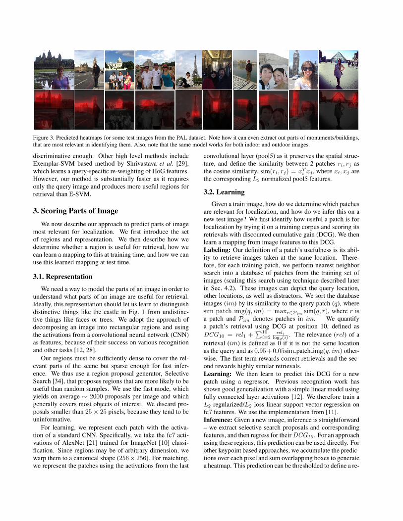
Figure 3. Predicted heatmaps for some test images from the PAL dataset. Note how it can even extract out parts of monuments/buildings,
that are most relevant in identifying them. Also, note that the same model works for both indoor and outdoor images.
discriminative enough. Other high level methods include
Exemplar-SVM based method by Shrivastava et al. [29],
which learns a query-specific re-weighting of HoG features.
However, our method is substantially faster as it requires
only the query image and produces more useful regions for
retrieval than E-SVM.
3. Scoring Parts of Image
We now describe our approach to predict parts of image
most relevant for localization. We first introduce the set
of regions and representation. We then describe how we
determine whether a region is useful for retrieval, how we
can learn a mapping to this at training time, and how we can
use this learned mapping at test time.
3.1. Representation
We need a way to model the parts of an image in order to
understand what parts of an image are useful for retrieval.
Ideally, this representation should let us learn to distinguish
distinctive things like the castle in Fig. 1 from undistinc-
tive things like faces or trees. We adopt the approach of
decomposing an image into rectangular regions and using
the activations from a convolutional neural network (CNN)
as features, because of their success on various recognition
and other tasks [12, 28].
Our regions must be sufficiently dense to cover the rel-
evant parts of the scene but sparse enough for fast infer-
ence. We thus use a region proposal generator, Selective
Search [34], that proposes regions that are more likely to be
useful than random samples. We use the fast mode, which
yields on average ∼ 2000 proposals per image and which
generally covers most objects of interest. We discard pro-
posals smaller than 25× 25 pixels, because they tend to be
uninformative.
For learning, we represent each patch with the activa-
tion of a standard CNN. Specifically, we take the fc7 acti-
vations of AlexNet [21] trained for ImageNet [10] classi-
fication. Since regions may be of arbitrary dimension, we
warp them to a canonical shape (256× 256). For matching,
we represent the patches using the activations from the last
convolutional layer (pool5) as it preserves the spatial struc-
ture, and define the similarity between 2 patches ri, rj as
the cosine similarity, sim(ri, rj) = xTi xj , where xi, xj are
the corresponding L2 normalized pool5 features.
3.2. Learning
Given a train image, how do we determine which patches
are relevant for localization, and how do we infer this on a
new test image? We first identify how useful a patch is for
localization by trying it on a training corpus and scoring its
retrievals with discounted cumulative gain (DCG). We then
learn a mapping from image features to this DCG.
Labeling: Our definition of a patch’s usefulness is its abil-
ity to retrieve images taken at the same location. There-
fore, for each training patch, we perform nearest neighbor
search into a database of patches from the training set of
images (scaling this search using technique described later
in Sec. 4.2). These images can depict the query location,
other locations, as well as distractors. We sort the database
images (im) by its similarity to the query patch (q), where
sim patch img(q, im) = maxr∈Pimsim(q, r), where r is
a patch and Pim denotes patches in im. We quantify
a patch’s retrieval using DCG at position 10, defined as
DCG10 = rel1 +∑10
i=2reli
log2(i) . The relevance (rel) of a
retrieval (im) is defined as 0 if it is not the same location
as the query and as 0.95+0.05sim patch img(q, im) other-
wise. The first term rewards correct retrievals and the sec-
ond rewards highly similar retrievals.
Learning: We then learn to predict this DCG for a new
patch using a regressor. Previous recognition work has
shown good generalization with a simple linear model using
fully connected layer activations [12]. We therefore train a
L2-regularized/L2-loss linear support vector regression on
fc7 features. We use the implementation from [11].
Inference: Given a new image, inference is straightforward
– we extract selective search proposals and corresponding
features, and then regress for their DCG10 . For an approach
using these regions, this prediction can be used directly. For
other keypoint based approaches, we accumulate the predic-
tions over each pixel and sum overlapping boxes to generate
a heatmap. This prediction can be thresholded to define a re-

Full
Im
age
- C
NN
F
ull
Im
age
- K
eyp
oin
t O
urs
Figure 4. This figure shows the prowess of our method compared to state of the art keypoint based approach [32], and CNN full image
features based approach. It shows the query on the top-left, and the top few retrievals using each of the approaches. Even when very little
of the Angkor Wat is visible, our method can hone in on the domes, and find other images taken at that place. Notice how the other methods
end up retrieving images of people, which are not really helpful in determining the location of the query image. Green and red borders
indicate correct and incorrect matches respectively.
gion of interest, just as query boxes are used on Oxford5K.
We show some results of these predictions in Fig. 3 and 9.
4. Retrieval Approaches
We now describe how the scoring method described
above can help improve an existing state-of-the art retrieval
approach [32]. We also propose a new approach to retrieval
using patches with the above scores that outperforms the
previous approaches by a large margin on our newly intro-
duced dataset, PAL.
4.1. Keypoint Features Based Retrieval
We use the recent approach from Tolias et al. [32] (using
the provided code) with the hessian affine detector [24] as
the baseline keypoint features based retrieval approach. It
already incorporates various recent advancements to mini-
mize the effect of ‘boring’ parts of image, such as handling
‘bursty’ [17] visual words. It has shown strong performance
on various datasets, including Oxford5K and Holidays. We
improve this base system using the scoring technique de-
scribed above in Sec. 3.
We improve [32] by defining a region-of-interest (RoI)
in the image, using the predicted heatmaps. Only fea-
tures inside the above RoI are used for retrieval. The
threshold for clipping the heatmap is learnt through grid
search over the training set. We define the region of in-
terest given a threshold t as area of the image satisfying
score > t × (max(hmap) − min(hmap)). We learn the
threshold for this (and other baseline methods, described in
Sec. 5.3) by computing the score heatmaps for the occluded
training images using a 10-fold cross validation output, and
performing retrieval over the complete train set. We per-
form grid search over threshold values (t) from 0 to 1, at
increment of 0.1, and for mean value of the heatmap, to
maximize mAP. We use these learnt thresholds directly for
Oxford5K as well.
4.2. CNN Feature Based Retrieval
In this section, we propose a novel approach to retrieval
using CNN features over patches of the image. To show
that its strong performance is not just because of the CNN
representation, we show that it can outperform a variety of
CNN-feature based baselines, including [14] that recently
introduced a new multiscale pooled feature representation
(MOP-CNN). This representation has been shown to per-
form well on various retrieval and recognition tasks, includ-
ing retrieval on the Holidays dataset.
CNN Patches Based Retrieval System Given a query
image, we decompose it into regions the exact same way as
at training time. We can perform two operations on each re-
gion: predict the DCG scores of the patch using the learned
model, and find similar patches in the corpus for the top
scoring patches. The question then becomes: How do we
use these to perform retrievals?
We propose the following model. Each query region
casts votes for each corpus image in proportion to the max-
imum similarity to the corpus image’s patches. We also in-
clude a vote from the full image retrieval, i.e. without using
patches. Hence, for a given image im1, the matching score
of each database image im2 is
sim img(im1, im2) +∑
p∈Pim1
sim patch img(p, im2)
where sim img(im1, im2) = sim(im1, im2), i.e. taking
the full image as a patch. This improves performance be-
cause it models global information, however as results in
Table 1 show, most of the improvement is obtained through
the patches. Thus, all that remains is to determine which
regions perform the lookups and vote. We select these re-
gions according to an objective that maximizes our rele-
vance subject to diversity, similar to [6]. Given a set of
regions S = {r1, . . . , r|S|}, our objective is
F (S) =∑
i
ψ(ri) + λ
(
maxj 6=i
sim(ri, rj)
)
where ψ(ri) is the unary score of a patch obtained from
the regressor, representing importance of that patch. In
other words, our set should have a high total score, but also
be diverse. Optimizing this is NP-hard, so we optimize it
greedily. We stop this procedure when we reach a pre-
determined number of patches (in all experiments, 5 – using
more patches gave better performance, but was slower). The
diversity trade-off parameter λ is learned via grid-search
from -5 to +5 with increments of 0.2 on the training set. We
observe through our experiments on PAL that λ is learned to
be -0.4, which means it penalizes similar patches. To avoid
over-fitting, the unaries used while learning λ are 10-fold
cross-validated output on the train set, same as in Sec 4.1.
Fig. 4 illustrates our approach and compares it to using only
full image features.
Scalability: Using CNN activations on patches is mem-
ory intensive: at 2000 per image, storing the pool5 fea-
tures of only a 1000 image dataset in memory would require
150GB of space. Hence, we use a dimensionality reduction
technique, Iterative Quantization [13] to hash the deep fea-
tures into 256-bit codes. This helps prune the search space
by actually matching the deep features only for the top-
1000 patches with least hamming distance in the hashed
space. We compress and store the actual features using a
read-optimized B+ tree implementation, LMDB, enabling
queries into a 3 million patch database within a few hun-
dred milliseconds on a single server. Note that this hashing
is only performed for our proposed patch based approach;
the baseline approaches (full image/MOPCNN) are unaf-
fected by this hashing.
5. Experiments and Results
We now present results to validate our approach. We
first introduce the “People at Landmarks” dataset, which
contains significant query image occlusion. We then show
that our patch scoring method can both improve [32], as
well as significantly outperform it using our CNN patch-
based approach on this dataset. Finally, we report results on
Oxford5K [26] which does not have heavy occlusion, but
still our method is able to improve the performance of [32]
and CNN-based method when not using the provided query
boxes.
5.1. People at Landmarks Dataset
To the best of our knowledge, no standard re-
trieval/localization dataset is composed of query images
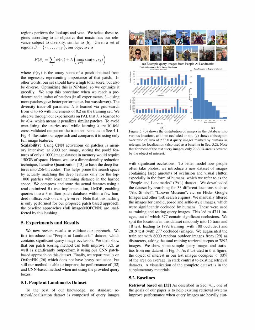
(a) Example query images from People At Landmarks
0
50
100
150
200
250
Nu
mb
er o
f Im
ages
People At Landmarks (PAL) Dataset Distribution Unoccluded Occluded
050
100150200250300350400450500
Nu
mb
er o
f Im
ages
Train Set
Test Set
0
10
20
30
40
50
60
70
80
0.1 0.2 0.3 0.4 0.5 0.6 0.7 0.8 0.9
Nu
mb
er o
f Im
ages
Ratio of Image Area
Area Occupied by Region of Interest
(b) (c)Figure 5. (b) shows the distribution of images in the database into
various locations, and into occluded or not. (c) shows a histogram
over ratio of area of 277 test query images marked by humans as
relevant for localization (also used as a baseline in Sec. 5.2). Note
that for most of the test query images, only 20-30% area is covered
by the object of interest.
with significant occlusions. To better model how people
often take photos, we introduce a new dataset of images
containing large amounts of occlusion and visual clutter,
especially in the form of humans, which we refer to as the
“People and Landmarks” (PAL) dataset. We downloaded
the dataset by searching for 33 different locations such as
“Abu Simbel”, “Louvre Museum”, etc. on Flickr, Google
Images and other web search engines. We manually filtered
the images for candid, posed and selfie-style images, which
were significantly occluded by humans. These were used
as training and testing query images. This led to 4711 im-
ages, out of which 377 contain significant occlusions. We
split the locations in this dataset randomly into 15 train and
18 test, leading to 1892 training (with 100 occluded) and
2819 test (with 277 occluded) images. We augmented the
train set with 6000 random outdoor images from [29] as
distractors, taking the total training retrieval corpus to 7892
images. We show some sample query images and statis-
tics from our dataset in Fig. 5. As illustrated in that figure,
the object of interest in our test images occupies < 30%of the area on average, in stark contrast to existing retrieval
datasets. A visualization of the complete dataset is in the
supplementary materials.
5.2. Baselines
Retrieval based on [32] As described in Sec. 4.1, one of
the goals of our paper is to help existing retrieval systems
improve performance when query images are heavily clut-

tered. We therefore apply our method to [32] and compare
with the following approaches for determining the impor-
tant image regions. We show a qualitative comparison of
each approach in Fig. 2.
(1) ESVM: Although it does not satisfy our computational
efficiency criterion (as scoring the query image takes many
hours), we use [29] to learn an exemplar-SVM that sepa-
rates the query image from background dataset. We then
convert the learned weights into a heatmap. We trained each
test image against the negative set containing 6000 random
outdoor images from [29]. The threshold was calibrated by
similarly computing heatmaps for the train images.
(2) Saliency: We use graph-based visual saliency (GBVS)
[16], which obtains strong performance. This checks
whether a non-task-specific notion of visual importance is
sufficient to identify informative regions for localization.
(3) Face-Detector: One large source of clutter in PAL is
faces; to verify our method is not just suppressing facial
clutter, we run a recent DPM-based face detector that ob-
tained state-of-the-art performance as of ECCV 14 [22]. We
tried two ways to suppress features. The first is within face
bounding boxes in order of score (Faces-BB). The second
is in order of distance to the nearest bounding box (Faces-
Dist).
(4) Human-Labeler: To attempt a comparison against hu-
mans, we asked two unaffiliated people to label a bounding
box they thought was most useful to recognize the place.
The images were shown in a random order and the subjects
were not familiar with the corpus.
CNN patches-based retrieval We compare our approach
described in Sec. 4.2 to using full image global CNN fea-
tures (layer pool5) over cosine distance metric. We also
compare with representations proposed in [14]: Layer-1
(full image fc7 features over Euclidean distance), Layer-
1+2 (full image, concatenated with 128 × 128 patches fea-
tures pooled using VLAD), and MOP-CNN (concatenation
of L-1+2 and 64× 64 patch features pooled similarly). We
used the provided code for [14].
5.3. Experimental Protocol
Performance Metrics: We use a variety of evaluation met-
rics. In addition to mean average precision (mAP) that
quantifies performance over all recall regimes, we use mean
precision (mP) at n for n = 1, 5, 10, 20 to characterize per-
formance among the top retrievals. For computing mP, we
ignore the exact match (query).
Protocol: Our method is learning-based and thus requires
held-out data. We train our models exclusively on the train-
ing set of PAL and test on the testing set of PAL. When test-
ing on Oxford5K, we apply models and thresholds learned
on PAL directly.
5.4. Results on People At Landmarks
We show some qualitative results of our method’s predic-
tions in Figure 6. It compares (a) MOPCNN with our CNN
← Top-Ranked Regions Bottom-Ranked Regions →
(a) Top and Bottom-Ranked Patches on PALPositive Weight Negative Weight
(b) Top activations of two positive and negatively ranked fc7 units
Figure 7. Analysis of our learned model. Note that our model
learns to reject faces, pavements, and gives high score to discrim-
inative parts of buildings.
patches based approach, and (b) keypoint based approach
[32] over full images with the same approach over image
regions determined by our method. Our method helps [32]
focus on the parts of the image that can help better localize
it, hence matching it to other images taken at the same loca-
tion. Our CNN patch based approach also gets much better
matches compared to MOPCNN [14].
We show qualitative analysis of our learned model in Fig.
7. In Fig. 7(a), we show the top-and bottom-ranked regions
on the training set: the top-ranked patches are not just non-
human, but also distinctive (e.g., the Leaning Tower, the
domes of Sacre-Coeur); the bottom-ranked patches natu-
rally correspond to people. We dig further into the model
in Fig. 7(b) by looking at the activations of two highly pos-
itive or negative feature dimensions. We scan the training
set for windows that most activate neurons corresponding
to highly positive and negatively-ranked dimensions. Di-
mensions with positive weight often contain buildings with
enough context to identify them; ones with negative weights
often contain people or regions that are too small to be dis-
tinguished.
We report quantitative results in Table 1. Our region
scoring method improves both base systems by a signifi-
cant margin, and our proposed CNN patch based approach
outperforms the state of the art retrieval approach of [32] by
> 10% mAP. Note that our performance is especially strong
in the high recall regimes (mP10 and mP20), presumably
because focusing on the landmark retrieves images where
the object of interest is not prominent, and hence is typically
missed when using the full image features. Improving [32]
using our predicted heatmaps, it also outperforms a number
of other schemes to determine a region-of-interest. A pre-
defined notion of importance, like saliency [16], harms per-
formance (because faces are typically predicted as impor-
tant by [16]). Similarly, the approach of [29] hurts perfor-
mance as it picks up on the coarse edges of the image (e.g.,
the edges of the Taj Mahal as opposed to its interior). Re-
moving faces and nearby regions helps, but only by a small
margin. Presumably, this is because [32] already accounts
for the frequency of faces through tf-idf and burstiness. On
the other hand, our method not only suppresses faces, but
determines what parts of the rest of the image to focus on.

Query Image MOP-CNN Our Approach (CNN)
Query Image Full Image (Keypoints) Our Approach (Keypoints)
(a)
(b)
Figure 6. This figure compares various retrieval approaches on the PAL dataset. (a) compares top retrievals using MOPCNN [14] and our
CNN patch based approach. (b) compares top retrievals using [32] and the same over regions selected using our method. Correct matches
are bordered with green.
Table 1. Results on PAL dataset. Using ESVM and Saliency to de-
fine a region-of-interest for [32] was found to harm performance
during cross-validation. Our proposed approach for [32] was de-
scribed in Sec. 4.1 and for CNN patches (Top-5 patch + full) in
Sec. 4.2.
mP1 mP5 mP10 mP20 mAP
Results using [32]
Full Image 91.7 85.2 78.5 68.5 29.6
Saliency [16] 91.7 85.2 78.5 68.5 29.6
Faces-BB 92.0 86.6 81.0 70.9 30.9
Faces-Dist 92.4 84.0 78.4 69.0 30.2
E-SVM [29] 91.7 85.2 78.5 68.5 29.6
Proposed 93.1 86.6 81.3 72.3 31.9
Human 91.7 88.4 83.1 73.9 33.0
Results using CNN patch-based retrieval
L-1 (fc7) [14] 57.0 47.4 41.0 35.3 21.3
L-1 (pool5) 61.4 51.5 45.4 39.9 21.6
L-1+2 [14] 61.0 51.0 45.1 38.5 23.1
MOP-CNN [14] 69.7 57.2 50.2 43.5 25.1
Top-1 patch 89.5 82.7 79.7 73.4 32.4
Top-5 patch 91.7 89.6 85.6 80.0 39.6
Top-5 + Full 92.8 89.2 85.7 80.5 40.3
Random-5 49.1 40.0 35.9 32.6 18.7
All Patches 75.1 65.3 60.9 55.6 31.5
For instance, our method prefers landmark-like structures
as opposed to generic buildings and definitely not pavement
or grass. As expected, human-marked boxes produce the
best results, but our method performs on par.
When using the CNN-patch based retrieval pipeline,
we outperform full image retrievals by 19%, and
MOPCNN [14] by 15% mAP. This shows that our improve-
ment can not solely be attributed to the CNN representa-
tion. It performs the best overall, outperforming [32] by
10.7%. We also ablatively compare our approach to using
just the top patch, and to top-5 patches without the full im-
age vote. We observe that most of the improvement is ob-
tained through the patches. Using random-5 patches or all
the patches performs worse, because a large part of the im-
age is irrelevant and their retrievals overwhelm the informa-
tive parts.
5.5. Natural Landmarks
Even though the PAL dataset already contains diverse
landmarks such as Trevi Fountain, Hollywood sign and Abu
Simbel, we explicitly verify our model’s ability to general-
ize to natural landmarks. To that end, we collect 1512 im-
ages from 3 natural landmarks, Grand Canyon, Half Dome
at Yosemite and Mount Rainier, and designate 25 images
with significant occlusion as test images. We use the PAL
trained model, without any re-training with identical pa-
rameters, to select regions on these images. Results are
in Table 2. We observe that our model trained on com-
pletely different data still gets similar or better performance
for both the baseline methods. We present some qualitative
results in the supplementary.
5.6. Results on Oxford5K
To further test whether our system can identify regions
that are useful for localization, we evaluate our approach
on Oxford5K [26] since it is well-known and dissimilar to
PAL. Oxford5K comes with manually marked query boxes
that identify objects of interest. Since these boxes already
identify useful regions and remove distractors, it is impossi-
ble to evaluate the system’s ability to identify useful regions

Table 2. Results on Natural Landmarks
mP1 mP5 mP10 mP20 mAP
Results using [32]
Full Image 96.0 81.6 73.6 67.6 40.1
Proposed 100.0 88.8 78.8 71.6 40.5
Results using CNN patch-based retrieval
L1 (pool5) 64.0 51.2 58.4 58.0 42.2
Top-5 + Full 84.0 79.2 79.6 78.6 45.0
CN
N F
ull
Im
age
CN
N t
op
-5 p
atch
*
Fu
ll I
mag
e H
eatm
ap th
resh
old
*
Border Color Key: Good OK Junk Bad
Figure 8. Top few retrievals for a sample query image in Oxford
Buildings, using (in order) [32], [32] with our predicted heatmaps
(proposed), CNN full image and CNN patch-based (proposed).
A ‘junk’ match in Oxford5K refers to matching images where
< 25% of the object is present.
while using the boxes: the task has already been done in
advance by the annotator. We therefore evaluate the system
on the full image, on which the base system performs worse
due to the distracting regions of image. We also note that in
many real-world applications, the user will not provide this
annotation. We show a qualitative result on an image more
similar to our PAL dataset in Fig. 8: the method success-
fully identifies the building as important, enabling the CNN
patch based approach to find 4 good matches, and using the
predicted heatmap with [32] gets three good matches. Com-
pared to using full image CNN and keypoint methods, this
performance is much better. We show some other heatmap
predictions on Oxford5K test images in Fig. 9.
Quantitatively, we observed a 77.37% mAP without us-
ing the query box, on modifying the provided code for [32]
to use our heatmaps, compared to 76.76% when using the
full image. The small gain on this dataset can be attributed
to the fact that most Oxford queries have the object of inter-
est covering most of the image, un-occluded. In the CNN
patches based approach, we observed an improvement of
Figure 9. Heatmaps predicted by our method on Oxford5K test
images using the model trained on PAL. It focuses on the main
object for localization, getting rid of people, cars, bicycles, generic
buildings and other boring parts of the image.
Table 3. Results on Oxford5K: Applying our PAL-learned model
directly to Oxford5K for selecting regions of the image, improves
retrieval performance by 0.61% for [32] and 22.2% for CNN.
Results using [32]
Without query box 76.76
Without query box, with histogram thresholding 77.37
With query box 80.64
Results using CNN patch-based retrieval
Full Image 37.74
Top-1 patch 50.30
Top-5 patch + Full 59.97
Top-50 patches 72.11
about 22% mAP over using full image features. Note that
for both the cases, the model was learned on PAL and ap-
plied directly to Oxford5K without any re-training and with
identical parameters. This shows the ability of our ap-
proach to easily and safely generalize across datasets, while
at worst preserving the original performance.
6. Conclusion
We have presented an approach that can zoom in and
determine which parts of the image are most useful for a
task and applied it to the task of localization through re-
trieval. We have also presented a novel approach to per-
forming retrieval using CNN features over patches of the
image. To help evaluate the approach, we introduced a new
dataset containing lots of visual clutter in the query images.
We showed that our proposed approach outperforms exist-
ing state of the art by more than 10% mAP for our newly
introduced dataset. Also, it improves the state of the art on
the Oxford5K dataset when not using the provided query
boxes.
Acknowledgements: This work was partially supported by
Siebel Scholarship to RG, Bosch Young Faculty Fellowship to AG
and NDSEG Fellowship to DF. This material is also based on re-
search partially sponsored by DARPA under agreement number
FA8750-14-2-0244. The U.S. Government is authorized to repro-
duce and distribute reprints for Governmental purposes notwith-
standing any copyright notation thereon. The views and conclu-
sions contained herein are those of the authors and should not be
interpreted as necessarily representing the official policies or en-
dorsements, either expressed or implied, of DARPA or the U.S.
Government.

References
[1] R. Arandjelovic and A. Zisserman. Multiple queries for large
scale specific object retrieval. In BMVC, 2012.
[2] R. Arandjelovic and A. Zisserman. Three things everyone
should know to improve object retrieval. In CVPR, 2012.
[3] R. Arandjelovic and A. Zisserman. All about VLAD. In
CVPR, 2013.
[4] R. Arandjelovic and A. Zisserman. DisLocation: Scalable
descriptor distinctiveness for location recognition. In ACCV,
2014.
[5] R. Arandjelovic and A. Zisserman. Visual vocabulary with a
semantic twist. In ACCV, 2014.
[6] D. Batra, P. Yadollahpour, A. Guzman-Rivera, and
G. Shakhnarovich. Diverse m-best solutions in markov ran-
dom fields. In ECCV, 2012.
[7] S. Cao and N. Snavely. Graph-based discriminative learning
for location recognition. In CVPR, 2013.
[8] O. Chum and J. Matas. Unsupervised discovery of co-
occurrence in sparse high dimensional data. In CVPR, 2010.
[9] O. Chum, J. Philbin, J. Sivic, M. Isard, and A. Zisserman.
Total recall: Automatic query expansion with a generative
feature model for object retrieval. In ICCV, 2007.
[10] J. Deng, W. Dong, R. Socher, L.-J. Li, K. Li, and L. Fei-Fei.
ImageNet: A Large-Scale Hierarchical Image Database. In
CVPR, 2009.
[11] R.-E. Fan, K.-W. Chang, C.-J. Hsieh, X.-R. Wang, and C.-J.
Lin. LIBLINEAR: A library for large linear classification.
JMLR, 2008.
[12] R. Girshick, J. Donahue, T. Darrell, and J. Malik. Rich fea-
ture hierarchies for accurate object detection and semantic
segmentation. In CVPR, 2014.
[13] Y. Gong and S. Lazebnik. Iterative quantization: A pro-
crustean approach to learning binary codes. In CVPR, 2011.
[14] Y. Gong, L. Wang, R. Guo, and S. Lazebnik. Multi-scale
orderless pooling of deep convolutional activation features.
In ECCV, 2014.
[15] P. Gronat, G. Obozinski, J. Sivic, and T. Pajdla. Learning and
calibrating per-location classifiers for visual place recogni-
tion. In CVPR, 2013.
[16] J. Harel, C. Koch, and P. Perona. Graph-based visual
saliency. In NIPS, 2006.
[17] H. Jegou, M. Douze, and C. Schmid. On the burstiness of
visual elements. In CVPR, 2009.
[18] H. Jegou, M. Douze, and C. Schmid. Improving bag-of-
features for large scale image search. IJCV, 2010.
[19] H. Jegou, F. Perronnin, M. Douze, J. Sanchez, P. Perez, and
C. Schmid. Aggregating local image descriptors into com-
pact codes. TPAMI, 2012.
[20] J. Knopp, J. Sivic, and T. Pajdla. Avoiding confusing features
in place recognition. In ECCV, 2010.
[21] A. Krizhevsky, I. Sutskever, and G. E. Hinton. Imagenet
classification with deep convolutional neural networks. In
NIPS, 2012.
[22] M. Mathias, R. Benenson, M. Pedersoli, and L. Van Gool.
Face detection without bells and whistles. In ECCV, 2014.
[23] A. Mikulık, M. Perdoch, O. Chum, and J. Matas. Learning a
fine vocabulary. In ECCV, 2010.
[24] M. Perdoch, O. Chum, and J. Matas. Efficient representation
of local geometry for large scale object retrieval. In CVPR,
2009.
[25] F. Perronnin, Y. Liu, J. Sanchez, and H. Poirier. Large-scale
image retrieval with compressed fisher vectors. In CVPR,
2010.
[26] J. Philbin, O. Chum, M. Isard, J. Sivic, and A. Zisser-
man. Object retrieval with large vocabularies and fast spatial
matching. In CVPR, 2007.
[27] J. Philbin, O. Chum, M. Isard, J. Sivic, and A. Zisserman.
Lost in quantization: Improving particular object retrieval in
large scale image databases. In CVPR, 2008.
[28] A. Razavian, H. Azizpour, J. Sullivan, and S. Carlsson. CNN
features off-the-shelf: an astounding baseline for recogni-
tion. CoRR, 2014.
[29] A. Shrivastava, T. Malisiewicz, A. Gupta, and A. A. Efros.
Data-driven visual similarity for cross-domain image match-
ing. SIGGRAPH ASIA, 2011.
[30] J. Sivic and A. Zisserman. Video google: A text retrieval
approach to object matching in videos. In ICCV, 2003.
[31] G. Tolias and Y. Avrithis. Speeded-up, relaxed spatial match-
ing. In ICCV, 2011.
[32] G. Tolias, Y. Avrithis, and H. Jegou. To aggregate or not
to aggregate: Selective match kernels for image search. In
ICCV, 2013.
[33] P. Turcot and D. Lowe. Better matching with fewer features:
The selection of useful features in large database recognition
problems. In ICCV Workshop (WS-LAVD), 2009.
[34] J. Uijlings, K. van de Sande, T. Gevers, and A. Smeulders.
Selective search for object recognition. ICCV, 2013.