CUTS AND FLOWS OF CELL COMPLEXES

CUTS AND FLOWS OF CELL COMPLEXES

ART M. DUVAL, CAROLINE J. KLIVANS, AND JEREMY L. MARTIN

Abstract. We study the vector spaces and integer lattices of cuts andflows associated with an arbitrary finite CW complex, and their rela-tionships to group invariants including the critical group of a complex.Our results extend to higher dimension the theory of cuts and flows ingraphs, most notably the work of Bacher, de la Harpe and Nagnibeda.We construct explicit bases for the cut and flow spaces, interpret theircoefficients topologically, and give sufficient conditions for them to beintegral bases of the cut and flow lattices. Second, we determine the pre-cise relationships between the discriminant groups of the cut and flowlattices and the higher critical and cocritical groups with error termscorresponding to torsion (co)homology. As an application, we general-ize a result of Kotani and Sunada to give bounds for the complexity,girth, and connectivity of a complex in terms of Hermite’s constant.

1. Introduction

This paper is about vector spaces and integer lattices of cuts and flowsassociated with a finite cell complex. Our primary motivation is the studyof critical groups of cell complexes and related group invariants. The crit-ical group of a graph is a finite abelian group whose order is the numberof spanning forests. The definition was introduced independently in severaldifferent settings, including arithmetic geometry [28], physics [12], and alge-braic geometry [2] (where it is also known as the Picard group or Jacobiangroup). It has received considerable recent attention for its connections todiscrete dynamical systems, tropical geometry, and linear systems of curves;see, e.g., [3, 4, 7, 22].

In previous work [17], the authors extended the definition of the criticalgroup to a cell complex Σ of arbitrary dimension. To summarize, the criticalgroup K(Σ) can be calculated using a reduced combinatorial Laplacian,

Date: August 12, 2014.2010 Mathematics Subject Classification. 05C05, 05C21, 05C50, 05E45, 11H06.Key words and phrases. cut lattice, flow lattice, critical group, spanning forest, cell

complex.Corresponding author: Art Duval, email [email protected].

Third author supported in part by a Simons Foundation Collaboration Grant and by Na-tional Security Agency grant no. H98230-12-1-0274. It is our pleasure to thank AndrewBerget, John Klein, Russell Lyons, Ezra Miller, Igor Pak, Dave Perkinson, and VictorReiner for valuable discussions, some of which took place at the 23rd International Con-ference on Formal Power Series and Algebraic Combinatorics (Reykjavik, 2011). We arealso grateful for the suggestions from an anonymous referee.

1

2 ART M. DUVAL, CAROLINE J. KLIVANS, AND JEREMY L. MARTIN

and its order is a weighted enumeration of the cellular spanning trees of Σ.Moreover, the action of the critical group on cellular (d−1)-cochains gives amodel of discrete flow on Σ, generalizing the chip-firing and sandpile models;see, e.g., [4, 12].

Bacher, de la Harpe, and Nagnibeda first defined the lattices C and F ofintegral cuts and flows for a graph [2]. By regarding a graph as an analogue ofa Riemann surface, they interpreted the discriminant groups C]/C and F ]/Frespectively as the Picard group of divisors and as the Jacobian group ofholomorphic forms. In particular, they showed that the critical group K(G)is isomorphic to both C]/C and F ]/F . Similar definitions and results appearin the work of Biggs [4].

In the present paper, we define the cut and flow spaces and cut and flowlattices of a cell complex Σ by

Cut(Σ) = imR ∂∗, Flow(Σ) = kerR ∂,

C(Σ) = imZ ∂∗, F(Σ) = kerZ ∂,

where ∂ and ∂∗ are the top cellular boundary and coboundary maps of Σ.In topological terms, cut- and flow-vectors are cellular coboundaries andcycles, respectively. Equivalently, the vectors in Cut(Σ) support sets offacets whose deletion increases the codimension-1 Betti number, and thevectors in Flow(Σ) support nontrivial rational homology classes.

In the higher-dimensional setting, the groups C]/C and F ]/F are not nec-essarily isomorphic to each other. Their precise relationship involves severalother groups: the critical group K(Σ), a dually defined cocritical groupK∗(Σ), and the cutflow group Zn/(C ⊕ F). We show that the critical andcocritical groups are respectively isomorphic to the discriminant groups ofthe cut lattice and flow lattice, and that the cutflow group mediates betweenthem with an “error term” given by homology. Specifically, if dim Σ = d,then we have the short exact sequences

0→ Zn/(C ⊕ F)→ C]/C ∼= K(Σ)→ T(Hd−1(Σ;Z))→ 0,

0→ T(Hd−1(Σ;Z))→ Zn/(C ⊕ F)→ F ]/F ∼= K∗(Σ)→ 0

(Theorems 7.6 and 7.7) where T denotes the torsion summand. The sizesof these groups are then given by

|C]/C| = |K(Σ)| = τ(Σ) = τ∗(Σ) · t2,

|F ]/F| = |K∗(Σ)| = τ∗(Σ) = τ(Σ)/t2,

|Zn/(C ⊕ F)| = τ(Σ)/t = τ∗(Σ) · t,

(Theorems 8.1 and 8.2), where t = |T(Hd−1(Σ;Z))| and τ(Σ) and τ∗(Σ) arethe weighted enumerators

τ(Σ) =∑Υ

|T(Hd−1(Υ;Z))|2, τ∗(Σ) =∑Υ

|T(Hd(Ω,Υ;Z))|2,

CUTS AND FLOWS OF CELL COMPLEXES 3

where both sums run over all cellular spanning forests Υ ⊆ Σ (see equa-tion (3)) and Ω is an acyclization of Υ (see Definition 7.3).

Before proving these results, we study the cut space (Section 4), the flowspace (Section 5), and the cut and flow lattices (Section 6) in some detail.In order to do this, we begin in Section 3 by describing and enumeratingcellular spanning forests of an arbitrary cell complex, generalizing our earlierwork [15, 16]. Similar results were independently achieved, using differenttechniques, by Catanzaro, Chernyak and Klein [8]. Our methods and resultsare very close to those of Lyons [29], but our technical emphasis is slightlydifferent.

Every cellular spanning forest Υ naturally gives rise to bases of the cutspace (Theorem 4.8) and the flow space (Theorem 5.5). In the graphic case,these basis vectors are simply signed characteristic vectors of fundamentalcocircuits and circuits in the graphic matroid, and they always form integralbases for the cut and flow lattices. For a general cellular complex, thesupports of basis vectors are given by cocircuits and circuits in the cellularmatroid of Σ (i.e., the matroid represented by the columns of ∂), but theirentries are not determined by the matroid. We prove that the basis vectorscan be scaled so that their entries are torsion coefficients of homology groupsof certain subcomplexes (Theorems 4.11 and 5.3). Under certain conditionson Υ, these bases are in fact integral bases for the cut and flow lattices(Theorems 6.1 and 6.2). Although the matroid data alone is not enoughto extend the theory of [2] to arbitrary cell complexes, the perspective ofmatroid theory will frequently be useful.

The idea of studying cuts and flows of matroids goes back to Tutte [33].More recently, Su and Wagner [32] define cuts and flows of a regular ma-troid (i.e., one represented by a totally unimodular matrix M); when M isthe boundary matrix of a cell complex, this is the case where the torsioncoefficients are all trivial. Su and Wagner’s definitions coincide with ours;their focus, however, is on recovering the structure of a matroid from themetric data of its flow lattice.

In the final section of the paper, we generalize a theorem of Kotani andSunada [26], who observed that a classical inequality for integer lattices,involving Hermite’s constant (see, e.g., [27]), could be applied to the flowlattice of a graph to give a bound for girth and complexity. We provethe corresponding result for cell complexes (Theorem 9.2), where “girth”means the size of a smallest circuit in the cellular matroid (or, topologically,the minimum number of facets supporting a nonzero homology class) and“complexity” is the torsion-weighted count of cellular spanning trees.

2. Preliminaries

In this section we review the tools needed throughout the paper: cellcomplexes, cellular spanning trees and forests, integer lattices, and matroids.


2.1. Cell complexes. Our work is motivated by algebraic graph theory,including critical groups, cut and flow spaces and lattices, and the chip-firing game. Our central goal is to extend the theory from graphs to higher-dimensional spaces. Thus we work in the setting of a finite CW complex,regarded as the higher-dimensional analogue of a graph. Accordingly, webegin by reviewing some of the topology of cell complexes; for a generalreference, see [23, p. 5]. The reader more familiar with simplicial complexesmay safely consider that special case throughout.

Throughout the paper, Σ will denote a finite CW complex (which we referto simply as a cell complex) of dimension d. We adopt the convention that Σhas a unique cell of dimension −1 (as though it were an abstract simplicialcomplex); this will allow our results to specialize correctly to the case d = 1(i.e., that Σ is a graph). We write Σi for the set of i-dimensional cells in Σ,and Σ(i) for the i-dimensional skeleton of Σ, i.e., Σ(i) = Σi ∪Σi−1 ∪ · · · ∪Σ0.Again, in keeping with simplicial-complex terminology, a cell of dimensiond is called a facet.

Unless otherwise stated, every d-dimensional subcomplex Γ ⊆ Σ will beassumed to have a full codimension-1 skeleton, i.e., Γ(d−1) = Σ(d−1). Accord-ingly, for simplicity of notation, we will often make no distinction betweenthe subcomplex Γ itself and its set Γd of facets.

The symbol Ci(Σ) = Ci(Σ;R) denotes the group of i-dimensional cellularchains with coefficients in a ring R. The i-dimensional cellular boundaryand coboundary maps are respectively ∂i(Σ;R) : Ci(Σ;R)→ Ci−1(Σ;R) and∂∗i (Σ;R) : Ci−1(Σ;R)→ Ci(Σ;R); we will write simply ∂i and ∂∗i wheneverpossible.

When Σ is a graph (i.e., a cell complex of dimension 1), its top boundarymap is a familiar object, namely its signed vertex-edge incidence matrix(with respect to some edge orientation). In this article, our goal will be toextract combinatorial information about an arbitrary cell complex from itstop-dimensional boundary map (which can be any integer matrix).

The ith reduced cellular homology and cohomology groups of Σ are re-spectively Hi(Σ;R) = ker ∂i/ im ∂i+1 and H i(Σ;R) = ker ∂∗i+1/ im ∂∗i . We

say that Σ is R-acyclic in codimension one if Hd−1(Σ;R) = 0. For a graph(d = 1), both Q- and Z-acyclicity in codimension one are equivalent to con-

nectedness. The ith reduced Betti number is βi(Σ) = dim Hi(Σ;Q), andthe ith torsion coefficient ti(Σ) is the cardinality of the torsion subgroup

T(Hi(Σ;Z)). We will frequently use the fact that

T(Hd−1(Σ;Z)) ∼= T(Hd(Σ;Z)) (1)

which is a special case of the universal coefficient theorem for cohomology[23, p. 205, Corollary 3.3]. A pair of complexes Γ ⊆ Σ induces a relative

complex (Σ,Γ), with relative homology and cohomology Hi(Σ,Γ;R) and

H i(Σ,Γ;R) and torsion coefficients ti(Σ,Γ) = |T(Hi(Σ,Γ;Z))|.


While many definitions and results can be stated purely algebraically(e.g., in terms of chain complexes over Z), we regard the underlying objectof interest as the cell complex (see Remark 4.2).

2.2. Spanning Forests and Laplacians. Our work on cuts and flows willuse the theory of spanning forests in arbitrary dimensions. Define a cellularspanning forest (CSF) of Σ to be a subcomplex Υ ⊆ Σ such that Υ(d−1) =Σ(d−1) and

Hd(Υ;Z) = 0, (2a)

rank Hd−1(Υ;Z) = rank Hd−1(Σ;Z), and (2b)

|Υd| = |Σd| − βd(Σ) (2c)

These conditions generalize the definition of a spanning forest1 of a graph G:respectively, it is acyclic, has c components, and has n−c edges, where n andc are the numbers of vertices and components of G. Just as in the graphiccase, any two of the conditions (2a), (2b), (2c) together imply the third; theproof is just a slight modification of the proof of [15, Proposition 3.5]. Anequivalent and perhaps simpler definition is that a subcomplex Υ ⊆ Σ is acellular spanning forest if and only if its d-cells correspond to a column basisfor the cellular boundary matrix ∂ = ∂d(Σ); however, the definition focusingon integral homology is frequently the most useful (see, e.g., Remark 4.15).

In the case that Σ is Q-acyclic in codimension one, this definition special-izes to our earlier definition of a cellular spanning tree [16, Definition 2.2].

There are two main reasons that enumeration of spanning forests of cellcomplexes is more complicated than for graphs. First, many properties ofgraphs can be studied component by component, so that one can usuallymake the simplifying assumption of connectedness; on the other hand, ahigher-dimensional cell complex cannot in general be decomposed into dis-joint pieces that are all acyclic in codimension one. Second, for complexes ofdimension greater than or equal to two, the possibility of torsion homologyaffects enumeration.

Define the ith up-down, down-up and total Laplacian operators2 on Σ by

Ludi = ∂i+1∂

∗i+1 : Ci(Σ;R)→ Ci(Σ;R),

Ldui = ∂∗i ∂i : Ci(Σ;R)→ Ci(Σ;R),

Ltoti = Lud

i + Ldui .

1That is, a maximal acyclic subgraph of G, not merely an acyclic subgraph containingall vertices.

2These are discrete versions of the Laplacian operators on differential forms of a Rie-mannian manifold. The interested reader is referred to [18] and [14] for their origins indifferential geometry and, e.g., [13, 20, 30] for more recent appearances in combinatorics.


Moreover, define the complexity of Σ as

τ(Σ) = τd(Σ) =∑

CSFs Υ⊆Σ

|T(Hd−1(Υ;Z))|2. (3)

The cellular matrix-tree theorem [16, Theorem 2.8] states that if Σ is Q-acyclic in codimension one and LΥ is the submatrix of Lud

d−1(Σ) obtainedby deleting the rows and columns corresponding to the facets of a (d − 1)-spanning tree Υ, then

τ(Σ) =|T(Hd−2(Σ;Z))|2

|T(Hd−2(Υ;Z))|2detLΥ.

In Section 3, we will generalize this formula to arbitrary cell complexes (i.e.,not requiring that Σ be Q-acyclic in codimension one). This has previouslybeen done by Lyons [29] in terms of slightly different invariants. If G is aconnected graph, then τ(G) is just the number of spanning trees, and werecover the classical matrix-tree theorem of Kirchhoff.

2.3. Lattices. Starting in Section 6, we will turn our attention to latticesof integer cuts and flows. We review some of the general theory of integerlattices; see, e.g., [1, Chapter 12], [21, Chapter 14], [24, Chapter IV].

A lattice L is a discrete subgroup of a finite-dimensional vector space V ;that is, it is the set of integer linear combinations of some basis of V . Everylattice L ⊆ Rn is isomorphic to Zr for some integer r ≤ n, called therank of L. The elements of L span a vector space denoted by L ⊗ R. ForL ⊆ Zn, the saturation of L is defined as L = (L ⊗ R) ∩ Zn. An integralbasis of L is a set of linearly independent vectors v1, . . . , vr ∈ L such thatL = c1v1+· · ·+crvr : ci ∈ Z. We will need the following fact about integralbases of lattices; the equivalences are easy consequences of the theory of freemodules (see, e.g., [1, Chapter 12], [24, Chapter IV]):

Proposition 2.1. For any lattice L ⊆ Zn, the following are equivalent:

(a) Every integral basis of L can be extended to an integral basis of Zn.(b) Some integral basis of L can be extended to an integral basis of Zn.(c) L is a summand of Zn, i.e., Zn can be written as an internal direct

sum L ⊕ L′.(d) L is the kernel of some group homomorphism Zn → Zm.

(e) L is saturated, i.e., L = L.(f) Zn/L is a free Z-module, i.e., its torsion submodule is zero.

Fixing the standard inner product 〈·, ·〉 on Rn, we define the dual latticeof L by

L] = v ∈ L ⊗ R : 〈v, w〉 ∈ Z ∀w ∈ L.Note that L] can be identified with the dual Z-module L∗ = Hom(L,Z), andthat (L])] = L. A lattice is called integral if it is contained in its dual; forinstance, any subgroup of Zn is an integral lattice. The discriminant group(or determinantal group) of an integral lattice L is L]/L; its cardinality


can be calculated as detMTM , for any matrix M whose columns form anintegral basis of L. We will need the following facts about bases and dualsof lattices.

Proposition 2.2. [21, Section 14.6] Let M be an n× r integer matrix.

(a) If the columns of M form an integral basis for the lattice L, then thecolumns of M(MTM)−1 form the corresponding dual basis for L].

(b) The matrix P = M(MTM)−1MT represents orthogonal projectionfrom Rn onto the column space of M .

(c) If the greatest common divisor of the r × r minors of M is 1, thenL] is generated by the columns of P .

2.4. The cellular matroid. Many ideas of the paper may be expressed effi-ciently using the language of matroids. For a general reference on matroids,see, e.g., [31]. We will primarily consider cellular matroids. The cellularmatroid of Σ is the matroid M(Σ) represented over R by the columns ofthe boundary matrix ∂. Thus the ground set of M(Σ) naturally corre-sponds to the d-dimensional cells Σd, and the matroid records which sets ofcolumns of ∂ are linearly independent. If Σ is a graph, then M(Σ) is itsusual graphic matroid, while if Σ is a simplicial complex then M(Σ) is itssimplicial matroid (see [10]).

The bases ofM(Σ) are the collections of facets of cellular spanning forestsof Σ. If r is the rank function of the matroidM(Σ), then for each set of facetsB ⊆ Σd, we have r(B) = rank ∂B, where ∂B is the submatrix consisting ofthe columns indexed by the facets in B. Moreover, we have

r(Σ) := r(Σd) = rankM(Σ) = rank ∂ = |Σd| − βd(Σ)

by the definition of Betti number.A set of facets B ⊆ Σd is called a cut if deleting B from Σ increases its

codimension-one homology, i.e., βd−1(Σ \ B) > βd−1(Σ). A cut B is a bondif r(Σ \B) = r(Σ)− 1, but r((Σ \B) ∪ σ) = r(Σ) for every σ ∈ B. That is,a bond is a minimal cut. In matroid terminology, a bond of Σ is preciselya cocircuit of M(Σ), i.e., a minimal set that meets every basis of M(Σ).Equivalently, a bond is the complement of a flat of rank r(Σ)− 1. If Υ is acellular spanning forest (i.e., a basis of M(Σ)) and σ ∈ Υd is a facet, thenthe fundamental bond of the pair (Υ, σ) is

bo(Υ, σ) = σ ∪ ρ ∈ Σd \Υ: Υ \ σ ∪ ρ is a CSF . (4)

This is the fundamental cocircuit of the pair (Υ, σ) of M(Σ) [31, p. 78].While the language of matroids will frequently be useful, it is important

to point out that most of the objects of interest to us, such as the cutand flow lattices and the critical group of a cell complex Σ, are not purelycombinatorial invariants of its cellular matroidM(Σ). (See [32] for more onthis subject, and [11, 19] for generalizations of matroids that contain finerarithmetic information). As an example, the summands in (3) are indexed


by the bases of M(Σ), but the summands themselves are not part of thematroid data. (On the other hand, when Σ is a graph, all summands are 1.)

Below is a table collecting some of the standard terminology from lin-ear algebra, graph theory, and matroid theory, along with the analogousconcepts that we will be using for cell complexes.

Linear algebra Graph Matroid Cell complex

Column vectors Edges Ground set FacetsIndependent set Acyclic subgraph Independent set Acyclic subcomplex

Min linear dependence Cycle Circuit Circuit

Basis Spanning forest Basis CSFSet meeting all bases Disconnecting set Codependent set Cut

Min set meeting all bases Bond Cocircuit Bond

Rank # edges in spanning forest Rank # facets in CSF

Here “codependent” means dependent in the dual matroid.

3. Enumerating Cellular Spanning Forests

In this section, we study the enumerative properties of cellular spanningforests of an arbitrary cell complex Σ. Our setup is essentially the same asthat of Lyons [29, §6], but the combinatorial formulas we will need later,namely Propositions 3.2 and 3.4, are somewhat different. As a corollary, weobtain an enumerative result, Proposition 3.5, which generalizes the simpli-cial and cellular matrix-tree theorems of [15] and [16] (in which we requiredthat Σ be Q-acyclic in codimension one). The result is closely related, butnot quite equivalent, to Lyons’ generalization of the cellular matrix-tree the-orem [29, Corollary 6.2], and to [8, Corollary D].

The arguments require some tools from homological algebra, in particularthe long exact sequence for relative homology and some facts about thetorsion-subgroup functor. The details of the proofs are not necessary tounderstand the constructions of cut and flow spaces in the later sections.

Let Σ be a d-dimensional cell complex with rank r. Let Γ ⊆ Σ be a sub-complex of dimension less than or equal to d− 1 such that Γ(d−2) = Σ(d−2).

Thus the inclusion map i : Γ → Σ induces isomorphisms i∗ : Hk(Γ;Q) →Hk(Σ;Q) for all k < d− 2.

Definition 3.1. The subcomplex Γ ⊆ Σ is called relatively acyclic if in factthe inclusion map i : Γ→ Σ induces isomorphisms i∗ : Hk(Γ;Q)→ Hk(Σ;Q)for all k < d.

By the long exact sequence for relative homology, Γ is relatively acyclic ifand only if Hd(Σ;Q)→ Hd(Σ,Γ;Q) is an isomorphism and Hk(Σ,Γ;Q) = 0for all k < d. These conditions can occur only if |Γd−1| = |Σd−1| − r. Thisquantity may be zero (in which case the only relatively acyclic subcomplexis Σ(d−2)). A relatively acyclic subcomplex is precisely the complement of a(d− 1)-cobase (a basis of the matroid represented over R by the rows of theboundary matrix ∂) in the terminology of Lyons [29].


Two special cases are worth noting. First, if d = 1, then a relativelyacyclic complex consists of one vertex in each connected component. Second,if Hd−1(Σ;Q) = 0, then Γ is relatively acyclic if and only if it is a cellularspanning forest of Σ(d−1).

For a matrix M , we write MA,B for the restriction of M to rows indexedby A and columns indexed by B.

Proposition 3.2. Let Γ ⊆ Υ ⊆ Σ be subcomplexes such that dim Υ = d;dim Γ = d− 1; |Υd| = r; |Γd−1| = |Σd−1| − r; Υ(d−1) = Σ(d−1); and Γ(d−2) =Σ(d−2). Also, let R = Σd−1 \ Γ. Then the following are equivalent:

(a) The r × r square matrix ∂ = ∂R,Υ is nonsingular.

(b) Hd(Υ,Γ;Q) = 0.

(c) Hd−1(Υ,Γ;Q) = 0.(d) Υ is a cellular spanning forest of Σ and Γ is relatively acyclic.

Proof. The cellular chain complex of the relative complex (Υ,Γ) is

0→ Cd(Υ,Γ;Q) = Qr ∂−→ Cd−1(Υ,Γ;Q) = Qr → 0

with other terms zero. If ∂ is nonsingular, then Hd(Υ,Γ;Q) and Hd−1(Υ,Γ;Q)are both zero; otherwise, both are nonzero. This proves the equivalence of(a), (b) and (c).

Next, note that Hd(Γ;Q) = 0 (because Γ has no cells in dimension d) and

that Hd−2(Υ,Γ;Q) = 0 (because Γ(d−2) = Υ(d−2)). Accordingly, the longexact sequence for relative homology of (Υ,Γ) is

0→ Hd(Υ;Q)→ Hd(Υ,Γ;Q)

→ Hd−1(Γ;Q)→ Hd−1(Υ;Q)→ Hd−1(Υ,Γ;Q)

→ Hd−2(Γ;Q)→ Hd−2(Υ;Q)→ 0.

(5)

If Hd(Υ,Γ;Q) = Hd−1(Υ,Γ;Q) = 0, then Hd(Υ;Q) = 0 (which says that Υis a cellular spanning forest) and the rest of (5) splits into two isomorphisms

that assert precisely that Γ is relatively acyclic (recall that Hd−1(Υ;Q) =

Hd−1(Σ;Q) when Υ is a cellular spanning forest). This implication is re-versible, completing the proof.

The torsion subgroup of a finitely generated abelian group A is defined asthe subgroup

T(A) = x ∈ A : kx = 0 for some k ∈ Z.

Note that A = T(A) if and only if A is finite. The torsion functor T is left-exact [24, p. 179]. Moreover, if A → B → C → 0 is exact and A = T(A),then T(A) → T(B) → T(C) → 0 is exact. We will need the followingadditional fact about the torsion functor.


Lemma 3.3. Suppose we have a commutative diagram of finitely generatedabelian groups

0 // Af //

α

Bg //

β

Ch //

Dj //

E //

0

0 // A′f ′ // B′

g′ // C ′h′ // D′

j′ // E′ // 0

(6)

such that both rows are exact; A,A′ are free; α is an isomorphism; β is sur-jective; and C,C ′ are finite. Then there is an induced commutative diagram

0 // TB ⊕G //

TC //

TD //

TE //

0

0 // TB′ ⊕G // TC ′ // TD′ // TE′ // 0

(7)

such that G is finite and both rows are exact. Consequently

|TB| · |TC ′| · |TD| · |TE′| = |TB′| · |TC| · |TD′| · |TE|. (8)

Proof. Since C is finite, we have ker j = imh ⊆ TD, so replacing D,E withtheir torsion summands preserves exactness. The same argument impliesthat we can replace D′, E′ with TD′,TE′.

Second, note that A,A′, B,B′ all have the same rank (since the rows areexact, C,C ′ are finite, and α is an isomorphism). Hence f(A) is a maximal-rank free submodule of B; we can write B = TB ⊕ F , where F is a freesummand of B containing f(A). Likewise, write B′ = TB′⊕F ′, where F ′ isa free summand of B′ containing f ′(A′). Meanwhile, β is surjective, hencemust restrict to an isomorphism F → F ′, which induces an isomorphismF/f(A) → F ′/f ′(A′). Abbreviating this last group by G, we obtain thedesired diagram (7) . Since ker g = im f ⊆ F , the map g : TB⊕G→ TC isinjective, proving exactness of the first row; the second row is exact by thesame argument. Exactness of each row implies that the alternating productof the cardinalities of the groups is 1, from which the formula (8) follows.

Proposition 3.4. Let Σ be a d-dimensional cell complex, let Υ ⊆ Σ bea cellular spanning forest, and let Γ ⊆ Σ be a relatively acyclic (d − 1)-subcomplex. Then

td−1(Υ) td−1(Σ,Γ) = td−1(Σ) td−1(Υ,Γ).

Proof. The inclusion Υ ⊆ Σ induces a commutative diagram

0 // Hd−1(Γ;Z)i∗ //

∼=

Hd−1(Υ;Z)j∗//

Hd−1(Υ,Γ;Z) //

Hd−2(Γ;Z) //

∼=

Hd−2(Υ;Z) //

∼=

0

0 // Hd−1(Γ;Z)i∗ // Hd−1(Σ;Z)

j∗// Hd−1(Σ,Γ;Z) // Hd−2(Γ;Z) // Hd−2(Σ;Z) // 0

whose rows come from the long exact sequences for relative homology. (For

the top row, the group Hd(Υ,Γ;Z) is free because dim Υ = d, and on theother hand is purely torsion by Proposition 3.2, so it must be zero. For


the bottom row, the condition that Γ is relatively acyclic implies that i∗is an isomorphism over Q; therefore, it is one-to-one over Z.) The groups

Hd−1(Υ,Γ;Z) and Hd−1(Σ,Γ;Z) are purely torsion. The first, fourth andfifth vertical maps are isomorphisms (the last because Υ(d−1) = Σ(d−1)) andthe second is a surjection by the relative homology sequence of the pair(Σ,Υ) (since the relative complex has no cells in dimension d − 1). Theresult now follows by applying Lemma 3.3 and canceling like terms.

As a consequence, we obtain a version of the cellular matrix-forest theo-rem that applies to all cell complexes (not only those that are Q-acyclic incodimension one).

Proposition 3.5. Let Σ be a d-dimensional cell complex and let Γ ⊆ Σbe a relatively acyclic (d − 1)-dimensional subcomplex, and let LΓ be therestriction of Lud

d−1(Σ) to the (d− 1)-cells of Γ. Then

τd(Σ) =td−1(Σ)2

td−1(Σ,Γ)2detLΓ.

Proof. By the Binet-Cauchy formula and Propositions 3.2 and 3.4, we have

detLΓ = det ∂Γ∂∗Γ =

∑Υ⊆Σd : |Υ|=r(Σ)

(det ∂Γ,Υ)2 =∑

CSFs Υ⊆Σd

td−1(Υ,Γ)2

=td−1(Σ,Γ)2

td−1(Σ)2

∑CSFs Υ⊆Σd

td−1(Υ)2 =td−1(Σ,Γ)2

td−1(Σ)2τd(Σ)

and solving for τd(Σ) gives the desired formula.

If Hd−1(Σ;Z) = T(Hd−1(Σ;Z)), then the relative homology sequence ofthe pair (Σ,Γ) gives rise to the exact sequence

0→ T(Hd−1(Σ;Z))→ T(Hd−1(Σ,Γ;Z))→ T(Hd−2(Γ;Z))→ T(Hd−2(Σ;Z))→ 0

which implies that td−1(Σ)/td−1(Σ,Γ) = td−2(Σ)/td−2(Γ), so Proposition 3.5

becomes the formula τd(Σ) =td−2(Σ)2

td−2(Γ)2 detLΓ. This was one of the original

versions of the cellular matrix-tree theorem [16, Theorem 2.8(2)].

Remark 3.6. Lyons [29, Corollary 6.2] proves a similar matrix-forest the-orem in terms of an invariant t′ defined below. He shows that each rowof (6) induces the corresponding row of (7). This does not quite implyLemma 3.3, since one still needs to identify the “error terms” G in thetop and bottom rows of (7). Doing so would amount to showing that

Hd−1(Υ)/ ker(j∗) ∼= Hd−1(Σ)/ ker(j∗) in the commutative diagram of Propo-sition 3.4. Alternatively, Proposition 3.4 would follow from [29, Lemma 6.1]together with the equation

td−2(Γ)t′d−1(Γ)/td−2(Σ) = td−1(Σ,Γ)/td−1(Σ)

where Γ = X(d−1) \ Γ and t′d−1(Γ) =∣∣ ker ∂d−1(Σ;Z)/

((ker ∂d−1(Σ;Z) ∩

im ∂d(Σ;Q)) + ker ∂d−1(Γ;Z))∣∣.


4. The Cut Space

Throughout this section, let Σ be a cell complex of dimension d and rank r(that is, every cellular spanning forest of Σ has r facets). For each i ≤ d,the i-cut space and i-flow space of Σ are defined respectively as the spacesof cellular coboundaries and cellular cycles:

Cuti(Σ) = im(∂∗i : Ci−1(Σ,R)→ Ci(Σ,R)),

Flowi(Σ) = ker(∂i : Ci(Σ,R)→ Ci−1(Σ,R)).

We will primarily be concerned with the case i = d. For i = 1, these are thestandard graph-theoretic cut and flow spaces of the 1-skeleton of Σ.

There are two natural ways to construct bases of the cut space of a graph,in which the basis elements correspond to either (a) vertex stars or (b) thefundamental circuits of a spanning forest (see, e.g. [21, Chapter 14]). Theformer is easy to generalize to cell complexes, but the latter takes morework.

First, if G is a graph on vertex set V and R is a set of (“root”) vertices,one in each connected component, then the rows of ∂ corresponding to thevertices V \R form a basis for Cut1(G). This observation generalizes easilyto cell complexes:

Proposition 4.1. A set of r rows of ∂ forms a row basis if and only if thecorresponding set of (d − 1)-cells is the complement of a relatively acyclic(d− 1)-subcomplex.

This is immediate from Proposition 3.2. Recall that if Hd−1(Σ;Q) = 0,then “relatively acyclic (d− 1)-subcomplex” is synonymous with “spanningtree of the (d − 1)-skeleton”. In this case, Proposition 4.1 is also a conse-quence of the fact that the matroid represented by the rows of ∂d is dual tothe matroid represented by the columns of ∂d−1 [16, Proposition 6.1].

The second way to construct a basis of the cut space of a graph is to fix aspanning tree and take the signed characteristic vectors of its fundamentalbonds. In the cellular setting, it is not hard to show that each bond supportsa unique (up to scaling) vector in the cut space (Lemma 4.4) and thatthe fundamental bonds of a fixed cellular spanning forest give rise to avector space basis (Theorem 4.8). (Recall from Section 2 that a bond ina cell complex is a minimal collection of facets whose removal increasesthe codimension-one homology, or equivalently a cocircuit of the cellularmatroid.) The hard part is to identify the entries of these cut-vectors. Fora graph, these entries are all 0 or ±1. In higher dimension, this need notbe the case, but the entries can be interpreted as the torsion coefficients ofcertain subcomplexes (Theorem 4.11). In Section 5, we will prove analogousresults for the flow space.

Remark 4.2. Although many of our results may be stated in terms ofalgebraic chain complexes over Z (integer boundary matrices), we use thelanguage of cell complexes. (This is a difference only in terminology, not the


generality of the results, since every integer matrix is the top-dimensionalboundary matrix of some cell complex.) Thus, definitions and results aboutcolumn bases, row bases, rank, etc., can be interpreted topologically in termsof cellular spanning trees and creating and puncturing holes in cell complexes(see Example 4.9 and Figure 1). This is analogous to the situation in al-gebraic graph theory, where results that can be stated in terms of matricesare often more significant in terms of trees, cuts, flows, etc.

4.1. A basis of cut-vectors. Recall that the support of a vector v =(v1, . . . , vn) ∈ Rn is the set

supp(v) = i ∈ [n] : vi 6= 0.

Proposition 4.3. [31, Proposition 9.2.4]. Let M be a r × n matrix withrowspace V ⊆ Rn, and let M be the matroid represented by the columnsof M . Then the cocircuits of M are the inclusion-minimal elements of thefamily Supp(V ) := supp(v) : v ∈ V \ 0.

Lemma 4.4. Let B be a bond of Σ. Then the set

CutB(Σ) = 0 ∪ v ∈ Cutd(Σ): supp(v) = Bis a one-dimensional subspace of Cutd(Σ). That is, up to scalar multiple,there is a unique cut-vector whose support is exactly B.

Proof. Suppose that v, w are vectors in the cut space, both supported on B,that are not scalar multiples of each other. Then there is a linear combina-tion of v, w with strictly smaller support; this contradicts Proposition 4.3.On the other hand, Proposition 4.3 also implies that CutB(Σ) is not thezero space; therefore, it has dimension 1.

We now know that for every bond B, there is a cut-vector supported on Bthat is uniquely determined up to a scalar multiple. As we will see, thereis a choice of scale so that the coefficients of this cut-vector are given bycertain minors of the down-up Laplacian L = Ldu

d (Σ) = ∂∗∂ (Lemma 4.6);these minors (up to sign) can be interpreted as the cardinalities of torsionhomology groups (Theorem 4.11).

In choosing a scale, the first step is to realize the elements of CutB(Σ)explicitly as images of the map ∂∗. Fix an inner product 〈·, ·〉 on each chaingroup Ci(Σ;R) by declaring the i-dimensional cells to be an orthonormalbasis. (This amounts to identifying each cell with the cochain that is itscharacteristic function.) Thus, for α ∈ Ci(Σ;R), we have supp(α) = σ ∈Σi : 〈σ, α〉 6= 0. Moreover, for all β ∈ Ci−1(Σ;R), we have by basic linearalgebra

〈∂α, β〉 = 〈α, ∂∗β〉 . (9)

Lemma 4.5. Let B be a bond of Σ and let U be the space spanned by∂σ : σ ∈ Σd \ B. In particular, U is a subspace of im ∂ of codimensionone. Let V be the orthogonal complement of U in im ∂, and let v be a nonzeroelement of V . Then supp(∂∗v) = B.


Proof. First, we show that ∂∗v 6= 0. To see this, observe that the columnspace of ∂ is U + Rv, so the column space of ∂∗∂ is ∂∗U + R∂∗v. However,rank(∂∗∂) = rank ∂ = r, and dimU = r − 1; therefore, ∂∗v cannot be thezero vector. Second, if σ ∈ Σd\B, then ∂σ ∈ U , so 〈∂∗v, σ〉 = 〈v, ∂σ〉 = 0. Itfollows that supp(∂∗v) ⊆ B, and in fact supp(∂∗v) = B by Proposition 4.3.

Given a bond B, let A = σ1, . . . , σr−1 be a cellular spanning forestof Σ \B. Fix a facet σ = σr ∈ B, so that A∪ σ is a cellular spanning forestof Σ. Define a vector

v = vA,σ =

r∑j=1

(−1)j(detLduA,A∪σ\σj )∂σj ∈ Cd−1(Σ;Z)

so that

∂∗v =r∑j=1

(−1)j(detLduA,A∪σ\σj )L

duσj ∈ Cutd(Σ). (10)

Lemma 4.6. For the cut-vector ∂∗v defined in equation (10),

∂∗v = (−1)r∑ρ∈B

(detLduA∪ρ,A∪σ)ρ.

In particular, supp(∂∗v) = B.

Proof. For each ρ ∈ B,

〈∂∗v, ρ〉 =r∑j=1

(−1)j detLduA,A∪σ\σj

⟨Lduσj , ρ

⟩=

r∑j=1

(−1)j detLduA,A∪σ\σj 〈∂σj , ∂ρ〉

=r∑j=1

(−1)j detLduA,A∪σ\σjL

duρ,σj

= (−1)r detLduA∪ρ,A∪σ,

where the last equality comes from expanding the row corresponding to ρ.Note that detLdu

A∪ρ,A∪σ 6= 0 for ρ = σ, so ∂∗v 6= 0. On the other hand,

by Cramer’s rule, v is orthogonal to ∂σ1, . . . , ∂σr−1, so in fact 〈∂∗v, ρ〉 = 0for all ρ ∈ Σd \ B. This establishes the desired formula for ∂∗v, and thensupp(∂∗v) = B by Lemma 4.5.

Equation (10) does not provide a canonical cut-vector associated to agiven bond B, because ∂∗v depends on the choice of A and σ. On the otherhand, the bond B can always be expressed as a fundamental bond bo(Υ, σ)(equivalently, fundamental cocircuit; see equation (4) in Section 2.4) bytaking σ to be an arbitrary facet of B and taking Υ = A ∪ σ, where Ais a maximal acyclic subset of Σ \ B. This observation suggests that the


underlying combinatorial data that gives rise to a cut-vector is really thepair (Υ, σ).

Definition 4.7. Let Υ = σ1, σ2, . . . , σr be a cellular spanning forest of Σ,and let σ = σi ∈ Υ. The (uncalibrated) characteristic vector of the bondbo(Υ, σ) is:

χ(Υ, σ) = (−1)rr∑j=1

(−1)j(detLduΥ\σ,Υ\σj )L

duσj

By Lemma 4.6, taking A = Υ \ σ, we have

χ(Υ, σ) =∑

ρ∈bo(Υ,σ)

(detLduΥ\σ∪ρ,Υ)ρ,

a cut-vector supported on bo(Υ, σ).

The next result is the cellular analogue of [21, Lemma 14.1.3].

Theorem 4.8. The family χ(Υ, σ) : σ ∈ Υ is an R-vector space basis forthe cut space of Σ.

Proof. Let σ ∈ Υ. Then supp χ(Υ, σ) = bo(Υ, σ) contains σ, but no otherfacet of Υ. Therefore, the set of characteristic vectors is linearly indepen-dent, and its cardinality is |Υd| = r = dim Cutd(Σ).

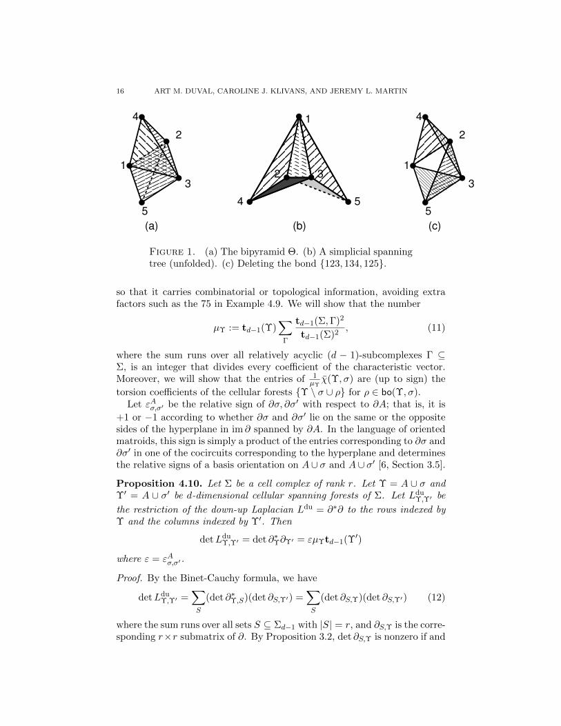
Example 4.9. The equatorial bipyramid is the two-dimensional simplicialcomplex Θ with facet set 123, 124, 125, 134, 135, 234, 235 (Figure 1(a)).Let Υ be the simplicial spanning tree with facets 123, 124, 234, 135, 235(unfolded in Figure 1(b)). Then

bo(Υ, 123) = 123, 125, 134, bo(Υ, 124) = 124, 134,bo(Υ, 135) = 135, 125, bo(Υ, 234) = 234, 134,bo(Υ, 235) = 235, 125.

In each case, the removal of the bond leaves a 1-dimensional hole (as shownfor the bond 123, 125, 134 in Figure 1(c)). By Theorem 4.8, we have

χ(Υ, 123) = 75([123] + [125]− [134]), χ(Υ, 124) = 75([124] + [134]),

χ(Υ, 135) = 75([125] + [135]), χ(Υ, 234) = 75([134] + [234]),

χ(Υ, 235) = 75([235]− [125]),

which indeed form a basis for Cut2(Θ).

4.2. Calibrating the characteristic vector of a bond. The term “char-acteristic vector” suggests that the coefficients of χ(Υ, σ) should all be 0or 1, but this is not necessarily possible, even by scaling, as Example 4.14below will show. We would like to define the characteristic vector of a bond


(a) (b) (c)

54

3

1

23

5

1

4

2

3

5

1

4

2

Figure 1. (a) The bipyramid Θ. (b) A simplicial spanningtree (unfolded). (c) Deleting the bond 123, 134, 125.

so that it carries combinatorial or topological information, avoiding extrafactors such as the 75 in Example 4.9. We will show that the number

µΥ := td−1(Υ)∑

Γ

td−1(Σ,Γ)2

td−1(Σ)2, (11)

where the sum runs over all relatively acyclic (d − 1)-subcomplexes Γ ⊆Σ, is an integer that divides every coefficient of the characteristic vector.Moreover, we will show that the entries of 1

µΥχ(Υ, σ) are (up to sign) the

torsion coefficients of the cellular forests Υ \ σ ∪ ρ for ρ ∈ bo(Υ, σ).Let εAσ,σ′ be the relative sign of ∂σ, ∂σ′ with respect to ∂A; that is, it is

+1 or −1 according to whether ∂σ and ∂σ′ lie on the same or the oppositesides of the hyperplane in im ∂ spanned by ∂A. In the language of orientedmatroids, this sign is simply a product of the entries corresponding to ∂σ and∂σ′ in one of the cocircuits corresponding to the hyperplane and determinesthe relative signs of a basis orientation on A∪ σ and A∪ σ′ [6, Section 3.5].

Proposition 4.10. Let Σ be a cell complex of rank r. Let Υ = A ∪ σ andΥ′ = A ∪ σ′ be d-dimensional cellular spanning forests of Σ. Let Ldu

Υ,Υ′ be

the restriction of the down-up Laplacian Ldu = ∂∗∂ to the rows indexed byΥ and the columns indexed by Υ′. Then

detLduΥ,Υ′ = det ∂∗Υ∂Υ′ = εµΥtd−1(Υ′)

where ε = εAσ,σ′.

Proof. By the Binet-Cauchy formula, we have

detLduΥ,Υ′ =

∑S

(det ∂∗Υ,S)(det ∂S,Υ′) =∑S

(det ∂S,Υ)(det ∂S,Υ′) (12)

where the sum runs over all sets S ⊆ Σd−1 with |S| = r, and ∂S,Υ is the corre-sponding r×r submatrix of ∂. By Proposition 3.2, det ∂S,Υ is nonzero if and


only if ΓS = Σd−1 \ S is relatively acyclic, and for those summands Propo-sition 3.4 implies | det ∂S,Υ| = td−1(Υ,ΓS) = td−1(Υ)td−1(Σ,ΓS)/td−1(Σ).

We claim that every summand in equation (12) has the same sign, namely ε.To see this, observe that since Υ,Υ′ are both column bases of ∂, there areunique scalars cα : α ∈ Υ such that ∂σ′ =

∑α∈Υ cα∂α; in particular, cσ

is nonzero and has the same sign as ε. This equation holds upon restrictingto any set of rows S. By linearity of the determinant, det ∂S,Υ′ = cσ det ∂S,Υfor each S, so the sign of every summand in (12) is the same as that of cσ.Therefore (12) gives

detLduΥ,Υ′ =

∑S

(det ∂S,Υ)(det ∂S,Υ′)

=∑S

ε

(td−1(Υ)td−1(Σ,ΓS)

td−1(Σ)

)(td−1(Υ′)td−1(Σ,ΓS)

td−1(Σ)

)= εµΥtd−1(Υ′).

A corollary of the proof is that µΥ is an integer, for the following reason.The number td−1(Υ′) is the gcd of the r × r minors of ∂Υ′ , or equivalentlythe r × r minors of ∂ using columns Υ′. In other words, td−1(Υ′) dividesdet ∂S,Υ′ in every summand of (12). Therefore it divides detLdu

Υ,Υ′ , and

µΥ = ±detLduΥ,Υ′/td−1(Υ′) is an integer.

Theorem 4.11. Let B be a bond. Fix a facet σ ∈ B and a cellular spanningforest A ⊆ Σd\B, so that in fact B = bo(A∪σ, σ). Define the characteristicvector of B with respect to A as

χA(B) :=1

µΥχ(A ∪ σ, σ) =

∑ρ∈B

εAσ,ρtd−1(A ∪ ρ) ρ.

Then χA(B) is in the cut space of Σ, and has integer coefficients. Moreover,it depends on the choice of σ only up to sign.

Proof. Apply the formula of Proposition 4.10 to the formula of Definition 4.7for the characteristic vector, and factor the integer µΥ out of every coeffi-cient. Meanwhile, replacing σ with a different facet σ′ ∈ B merely multipliesall coefficients by εAσ′,ρ/ε

Aσ,ρ = εAσ,σ′ ∈ ±1.

Remark 4.12. We are grateful to an anonymous referee for suggesting thefollowing construction of the vector χA(B). Let M ∈ Zk×n be a matrixof rank r whose first r columns are linearly independent, and let P be thegeneralized inverse of the submatrix of M consisting of the first r columns,so that Q = PM is the reduced row-echelon form of M . Thus P−1Q = M .By Cramer’s rule, for each j ∈ [n], the jth entry in the rth row of Q is

qr,j =det(m1, . . . ,mr−1,mj)

det(m1, . . . ,mr−1,mr),

where mi denotes the ith column of M .


Now let Σ, B,A, σ be as in Theorem 4.11, let r = rank(Σ), and let M bethe top boundary matrix of Σ, with its first r − 1 columns labeled by thefacets of A and the rth column labeled by σ. The numerator of qr,j is

0 for j 6∈ B,εAσ,ρjtd−1(A ∪ ρj) for j ∈ B,

where ρj denotes the facet corresponding to the jth column. Therefore,

clearing the denominators from the rth row of M produces the characteristicvector χA(B) of Theorem 4.11.

If Υ is a cellular spanning forest of Σ and σ ∈ Υd, then we define thecharacteristic vector of the pair (Υ, σ) by

χ(Υ, σ) := χΥ\σ(bo(Υ, σ)) =1

µΥχ(Υ, σ). (13)

Example 4.13. Let Θ be the bipyramid of Example 4.9. Every cellularspanning forest Υ ⊆ Θ is torsion-free. Moreover, the relatively acyclic sub-complexes Γ that appear in equation (11) are the spanning trees of the 1-skeleton Θ(1) (see Section 3), which is the graph K5 with one edge removed;Accordingly, we have µΥ = τ(Θ(1)) = 75, so the calibrated characteristicvectors are as in Example 4.9, with all factors of 75 removed.

On the other hand, µΥ is not necessarily the greatest common factor of theentries of each uncalibrated characteristic vector, as the following exampleillustrates.

Example 4.14. Consider the cell complex Σ with a single vertex v, two1-cells e1 and e2 attached at v, and four 2-cells attached via the boundarymatrix

∂ =

(σ2 σ3 σ5 σ7

e1 2 3 0 0e2 0 0 5 7

).

Let B be the bond σ2, σ3, so that the obvious candidate for a cut-vectorsupported on B is the row vector

[2 3 0 0

]. On the other hand, taking

A = σ5 (a cellular spanning forest of Σ \B), the calibrated characteristicvector given by Theorem 4.11 is

χA(B) =[10 15 0 0

].

For Υ = A∪ σ2, the uncalibrated characteristic vector of Definition 4.7 is

χ(Υ, σ2) =[100 150 0 0

].

On the other hand, the calibration factor µΥ is not gcd(100, 150) = 50, butrather 10, since t1(Υ) = 10 and the summation of equation (11) has onlyone term, namely Γ = Σ(0). Similarly, for A′ = σ7 and Υ′ = A′ ∪σ2, wehave

χA′(B) =[14 21 0 0

], χ(Υ′, σ2) =

[196 294 0 0

], µΥ′ = 14.


Remark 4.15. As an illustration of where torsion plays a role, and of theprinciple that the cellular matroid M(Σ) does not provide complete infor-mation about cut-vectors, let Σ be the the complete 2-dimensional simplicialcomplex on 6 vertices, which has complexity 66 = 46656 [25, Theorem 1].Most of the cellular spanning trees of Σ are contractible topological spaces,hence Z-acyclic, and the calibrated cut-vectors obtained from them have allentries equal to 0 or ±1. On the other hand, Σ has twelve spanning treesΥ homeomorphic to the real projective plane (so that H1(Υ;Z) ∼= Z2). Forany facet σ ∈ Υ, we have bo(Υ, σ) = Σ2 \ Υ2 ∪ σ, and the calibratedcut-vector contains a ±2 in position σ and ±1’s in positions Σ \Υ.

Remark 4.16. When Σ is a graph and Υ is a spanning forest, µΥ is justthe number of vertices of Σ. Then, for any edge σ in Υ, the vector χΥ(σ) isthe usual characteristic vector of the fundamental bond bo(Υ, σ).

Remark 4.17. Taking Υ = Υ′ in the calculation of Proposition 4.10 givesthe equality ∑

Γ

td−1(Σ,Γ)2 =td−1(Σ)2

td−1(Υ)2detLdu

Υ

which can be viewed as a dual form of Proposition 3.5, enumerating relativelyacyclic (d− 1)-subcomplexes, rather than cellular spanning forests.

5. The Flow Space

In this section we describe the flow space of a cell complex. We begin byobserving that the cut and flow spaces are orthogonal to each other.

Proposition 5.1. The cut and flow spaces are orthogonal complements un-der the standard inner product on Cd(Σ;R).

Proof. First, we show that the cut and flow spaces are orthogonal. Letα ∈ Cutd = im ∂∗d and β ∈ Flowd = ker ∂d. Then α = ∂∗γ for some (d− 1)-chain γ, and 〈α, β〉 = 〈∂∗γ, β〉 = 〈γ, ∂β〉 = 0 by equation (9).

It remains to show that Cutd and Flowd have complementary dimen-sions. Indeed, let n = dimCd(Σ;R); then dim Flowd = dim ker ∂d = n −dim im ∂d = n− dim im ∂∗d = n− dim Cutd.

Next we construct a basis of the flow space whose elements correspondto fundamental circuits of a given cellular spanning forest. Although cutsand flows are in some sense dual constructions, it is easier in this case towork with kernels than images, essentially because of Proposition 2.1. As aconsequence, we can much more directly obtain a characteristic flow vectorwhose coefficients carry topological meaning.

We need one preliminary result from linear algebra.

Proposition 5.2. Let N be an r × c integer matrix of rank c− 1 such thatevery set of c − 1 columns is linearly independent, so that r ≥ c − 1 anddim kerN = 1. Then kerN has a spanning vector v = (v1, . . . , vc) such that

vi = ±|T(cokerNı)|


where Nı denotes the submatrix of N obtained by deleting the ith column.In particular, vi 6= 0 for all i.

Proof. Let Q be an r×r matrix whose first r−(c−1) rows form a Z-modulebasis for ker(NT ), and whose remaining c − 1 rows extend it to a basisof Zr (see Proposition 2.1). Then Q is invertible over Z, and the matrixP = QN = (NTQT )T has the form

P =

[0M

]where M is a (c − 1) × c matrix whose column matroid is the same asthat of N . Then kerN = kerP = kerM . Meanwhile, by Cramer’s rule,kerM is the one-dimensional space spanned by v = (v1, . . . , vc), wherevi = (−1)i detMı = ±| cokerMı| = ±|T(cokerPı)|. Since Q is invert-ible, it induces isomorphisms cokerNı

∼= cokerQNı = cokerPı for all i,so |T(cokerPı)| = |T(cokerNı)|, completing the proof.

Recall that a set of facets C ⊆ Σd is a circuit of the cellular matroidM(Σ) if and only if it corresponds to a minimal linearly dependent set ofcolumns of ∂d. Applying Proposition 5.2 with N = ∂C (i.e., the restrictionof ∂ to the columns indexed by C), we obtain a flow vector whose supportis exactly C. We call this the characteristic vector ϕ(C).

Theorem 5.3. Let C be a circuit of the cellular matroid M(Σ), and let∆ ⊆ Σ be the subcomplex Σ(d−1) ∪ C. Then

ϕ(C) =∑σ∈C±td−1(∆ \ σ)σ.

Proof. Let N = ∂C , and for σ ∈ C, let Nσ denote N with the column σremoved. By Proposition 5.2, it suffices to show that the two groups

Hd−1(∆ \ σ;Z) =ker ∂d−1

imNσ, cokerNσ =

Cd−1(Σ;Z)

imNσ

have the same torsion summands. But this is immediate because ker ∂d−1 isa summand of Cd−1(Σ;Z) as a free Z-module.

Example 5.4. Consider the cell complex Σ with two vertices v1 and v2,three one-cells e1, e2, and e3, each one with endpoints v1 and v2, and threetwo-cells σ1, σ2, and σ3 attached to the one-cells so that the 2-dimensionalboundary matrix is

∂ =

σ1 σ2 σ3

e1 2 2 0e2 −2 0 1e3 0 −2 −1

.The only circuit in Σ is the set C of all three two-cells. Thus ϕ(C) = 2σ1 −2σ2 + 4σ3, because the relevant integer homology groups are H1(∆ \ σ1) ∼=H1(∆ \ σ2) ∼= Z2, but H1(∆ \ σ3) ∼= Z2 ⊕ Z2.


For a cellular spanning forest Υ and facet σ 6∈ Υ, let ci(Υ, σ) denote thefundamental circuit of σ with respect to Υ, that is, the unique circuit inΥ ∪ σ.

Theorem 5.5. Let Σ be a cell complex and Υ ⊆ Σ a cellular spanningforest. Then the set

ϕ(ci(Υ, σ)) : σ 6∈ Υforms an R-vector space basis for the flow space of Σ.

Proof. The flow space is the kernel of a matrix with |Σd| columns and rank|Υd|, so its dimension is |Σd|−|Υd|. Therefore, it is enough to show that theϕ(ci(Υ, σ)) are linearly independent. Indeed, consider the matrix W whoserows are the vectors ϕ(ci(Υ, σ)); its maximal square submatrix W ′ whosecolumns correspond to Σ \Υ has nonzero entries on the diagonal but zeroeselsewhere.

Example 5.6. Recall the bipyramid of Example 4.9, and its spanning treeΥ. Then ci(Υ, 125) = 125, 123, 135, 235, and ci(Υ, 134) = 134, 123, 124, 234.If we instead consider the spanning tree Υ′ = 124, 125, 134, 135, 235, thenci(Υ′, 123) = 123, 125, 135, 235, and ci(Υ′, 234) = 234, 124, 125, 134, 135, 235.Each of these circuits is homeomorphic to a 2-sphere, and the correspondingflow vectors are the homology classes they determine. Furthermore, each ofϕ(ci(Υ, 125)), ϕ(ci(Υ, 134)) and ϕ(ci(Υ′, 123)), ϕ(ci(Υ′, 234)) is a basisof the flow space.

6. Integral Bases for the Cut and Flow Lattices

Recall that the cut lattice and flow lattice of Σ are defined as

C = C(Σ) = imZ ∂∗d ⊆ Zn, F = F(Σ) = kerZ ∂d ⊆ Zn.

In this section, we study the conditions under which the vector space basesof Theorems 4.11 and 5.5 are integral bases for the cut and flow latticesrespectively.

Theorem 6.1. Suppose that Σ has a cellular spanning forest Υ such thatHd−1(Υ;Z) is torsion-free. Then

χ(Υ, σ) : σ ∈ Υis an integral basis for the cut lattice C(Σ), where χ(Υ, σ) is defined as inequation (13).

Proof. Consider the n × r matrix with columns χ(Υ, σ) for σ ∈ Υd. Itsrestriction to the rows Υd is diagonal, and by Theorem 4.8 and the hypoth-esis on Hd−1(Υ;Z), its entries are all ±1. Therefore, the χ(Υ, σ) form anintegral basis for the lattice Cutd(Σ) ∩ Zn. Meanwhile,

(Cutd(Σ) ∩ Zn)/Cd(Σ) = T(Hd(Σ;Z)) ∼= T(Hd−1(Σ;Z))

where the first equality is because Cutd(Σ) ∩ Zn is a summand of Zn, and

the second one is equation (1). On the other hand, Hd−1(Σ;Z) is a quotient


of Hd−1(Υ;Z) of equal rank; in particular, T(Hd−1(Σ;Z)) = 0 and in factCutd(Σ) ∩ Zn = Cd(Σ).

Next we consider integral bases of the flow lattice. For a circuit C, define

ϕ(C) =1

gϕ(C)

where ϕ(C) is the characteristic vector defined in Section 5 and g is the gcdof its coefficients. Thus ϕ(C) generates the rank-1 free Z-module of flowvectors supported on C.

Theorem 6.2. Suppose that Σ has a cellular spanning forest Υ such thatHd−1(Υ;Z) = Hd−1(Σ;Z). Then ϕ(ci(Υ, σ)) : σ 6∈ Υ is an integral basisfor the flow lattice F(Σ).

Proof. By the hypothesis on Υ, the columns of ∂ indexed by the facetsin Υ form a Z-basis for the column space. That is, for every σ 6∈ Υ, thecolumn ∂σ is a Z-linear combination of the columns of Υ; equivalently, thereis an element wσ of the flow lattice, with support ci(Υ, σ), whose coefficientin the σ position is ±1. But then wσ and ϕ(ci(Υ, σ)) are integer vectors withthe same linear span, both of which have the gcd of their entries equal to 1;therefore, they must be equal up to sign. Therefore, retaining the notationof Theorem 5.5, the matrix W ′ is in fact the identity matrix, and it followsthat the lattice spanned by the ϕ(ci(Υ, σ)) is saturated, so it must equal theflow lattice of Σ.

If Σ is a graph, then all its subcomplexes and relative complexes aretorsion-free (equivalently, its incidence matrix is totally unimodular). There-fore, Theorems 6.1 and 6.2 give integral bases for the cut and flow latticesrespectively. These are, up to sign, the integral bases constructed combina-torially in, e.g., [21, Chapter 14].

7. Groups and Lattices

In this section, we define the critical, cocritical, and cutflow groups of acell complex. We identify the relationships between these groups and to thediscriminant groups of the cut and flow lattices. The case of a graph wasstudied in detail by Bacher, de la Harpe and Nagnibeda [2] and Biggs [4],and is presented concisely in [21, Chapter 14].

Throughout this section, let Σ be a cell complex of dimension d with nfacets, and identify both Cd(Σ;Z) and Cd(Σ;Z) with Zn.

Definition 7.1. The critical group of Σ is

K(Σ) := T(ker ∂d−1/ im ∂d∂∗d) = T(coker(∂d∂

∗d)).

Here and henceforth, all kernels and images are taken over Z.

Note that the second and third terms in the definition are equivalentbecause ker ∂d−1 is a summand of Cd−1(Σ;Z) as a free Z-module. Thisdefinition coincides with the usual definition of the critical group of a graph


in the case d = 1, and with the authors’ previous definition in [17] in thecase that Σ is Q-acyclic in codimension one (when ker ∂d−1/ im ∂d∂

∗d is its

own torsion summand).

Definition 7.2. The cutflow group of Σ is Zn/(C(Σ)⊕F(Σ)).

Note that the cutflow group is finite because the cut and flow spaces areorthogonal complements in Rn (Proposition 5.1), so in particular C ⊕ Fspans Rn as a vector space. Observe also that the cutflow group does notdecompose into separate cut and flow pieces; that is, it is not isomorphic tothe group G = ((Flowd ∩Zn)/ ker ∂d)⊕ ((Cutd ∩Zn)/ im ∂∗d), even when Σ isa graph. For example, if Σ is the complete graph on three vertices, whoseboundary map can be written as

∂ =

1 −1 0−1 0 10 1 −1

,

then ker ∂ = span(1, 1, 1)T and im ∂∗ = span(1,−1, 0)T , (1, 0,−1)T . SoG is the trivial group, while Zn/(ker ∂d ⊕ im ∂∗d) = K1(Σ) ∼= Z3.

In order to define the cocritical group of a cell complex, we first need tointroduce the notion of acyclization.

Definition 7.3. An acyclization of Σ is a (d + 1)-dimensional complex Ω

such that Ω(d) = Σ and Hd+1(Ω;Z) = Hd(Ω;Z) = 0.

Algebraically, this construction corresponds to finding an integral basisfor ker ∂d(Σ) and declaring its elements to be the columns of ∂d+1(Ω) (so

in particular |Ω(d+1)| = βd(Σ)). Topologically, it corresponds to filling injust enough d-dimensional cycles with (d + 1)-dimensional faces to removeall d-dimensional homology. The definition of acyclization and equation (1)

together imply that Hd+1(Ω;Z) = 0; that is, ∂∗d+1(Ω) is surjective.

Definition 7.4. The cocritical group K∗(Σ) is

K∗(Σ) := Cd+1(Ω;Z)/ im ∂∗d+1∂d+1 = cokerLdud+1.

It is not immediate that the groupK∗(Σ) is independent of the choice of Ω;we will prove this independence as part of Theorem 7.7. For the moment,it is at least clear that K∗(Σ) is finite, since rank ∂∗d+1 = rankLdu

d+1 =

rankCd+1(Ω;Z). In the special case of a graph, Ldud+1 is the “intersection

matrix” defined by Kotani and Sunada [26]. (See also [5, Sections 2, 3].)

Remark 7.5. As in [17], one can define critical and cocritical groups in everydimension byKi(Σ) = T(Ci(Σ;Z)/ im ∂i+1∂

∗i+1) andK∗i (Σ) = T(Ci(Σ;Z)/ im ∂∗i ∂i).

If the cellular chain complexes of Σ and Ψ are algebraically dual (for exam-ple, if Σ and Ψ are Poincare dual cell structures on a compact orientabled-manifold), then Ki(Ψ) = K∗d−i(Σ) for all i.

We now come to the main results of the second half of the paper: thecritical and cocritical groups are isomorphic to the discriminant groups of the


cut and flow lattices respectively, and the cutflow group mediates betweenthe critical and cocritical groups, with an “error term” given by homology.

Theorem 7.6. Let Σ be a cell complex of dimension d with n facets. Thenthere is a commutative diagram

0 // Zn/(C ⊕ F)

α

ψ // C]/C

β

// T(Hd(Σ;Z))

γ

// 0

0 // im ∂d/ im ∂d∂∗d

// K(Σ) // T(Hd−1(Σ;Z)) // 0

(14)

in which all vertical maps are isomorphisms. In particular, K(Σ) ∼= C]/C.

Proof. Step 1: Construct the bottom row of (14). The inclusions im ∂d∂∗d ⊆

im ∂d ⊆ ker ∂d−1 give rise to the short exact sequence

0→ im ∂d/ im ∂d∂∗d → ker ∂d−1/ im ∂d∂

∗d → ker ∂d−1/ im ∂d → 0.

The first term is finite (because rank ∂d = rank ∂d∂∗d), so taking torsion

summands yields the desired short exact sequence.Step 2: Construct the top row of (14). Let r = rank ∂d, let v1, . . . , vr

be an integral basis of C, and let V be the matrix with columns v1, . . . , vr.By Proposition 2.2, the dual basis v∗1, . . . , v∗r for C] consists of the columnsof the matrix W = V (V TV )−1. Let ψ be the orthogonal projection Rn →Cut(Σ), which is given by the matrix P = WV T = V (V TV )−1V T (seeProposition 2.2). Then

imψ = colspace

[v∗1 · · · v∗r]︸︷︷︸W

[v1 · · · vr

]T︸︷︷︸V T

.

The ith column of P equals W times the ith column of V T . If we identifyC] with Zr via the basis v∗1, . . . , v∗r, then im(ψ) is just the column spaceof V T . So C]/ imψ ∼= Zr/ colspace(V T ), which is a finite group becauserankV = r. Since the matrices V and V T have the same invariant factors,we have

Zr/ colspace(V T ) ∼= T(Zn/ colspace(V )) = T(Cd(Σ;Z)/ im ∂∗d) = T(Hd(Σ;Z)).

Meanwhile, imψ ⊇ C because PV = V . Since kerψ = F , we have (imψ)/C =(Zn/F)/C = Zn/(C ⊕ F). Therefore, the inclusions C ⊆ imψ ⊆ C] give riseto the short exact sequence in the top row of (14).

Step 3: Describe the vertical maps in (14). The maps α and β are eachinduced by ∂d in the following ways. First, the image of the cutflow groupunder ∂d is

∂d (Zn/(F ⊕ C)) = ∂d (Zn/(ker ∂d ⊕ im ∂∗d)) = im ∂d/ im ∂d∂∗d .

On the other hand, ∂d acts injectively on the cutflow group (since the latteris a subquotient of Zn/ ker ∂d). So the map labeled α is an isomorphism.


The cellular boundary map ∂d also gives rise to the map β : C]/C → K(Σ),as we now explain. First, note that ∂d C] ⊆ imR ∂d ⊆ kerR ∂d−1. Second,observe that for every w ∈ C] and ρ ∈ Cd−1(Σ;Z), we have 〈∂w, ρ〉 =〈w, ∂∗ρ〉 ∈ Z, by equation (9) and the definition of dual lattice. Therefore,∂d C] ⊆ Cd−1(Σ;Z). It follows that ∂d maps C] to (kerR ∂d−1)∩Cd−1(Σ;Z) =kerZ ∂d−1, hence defines a map β : C]/C → kerZ ∂d−1/ imZ ∂d∂

∗d . Since C]/C is

finite, the image of β is purely torsion, hence contained in K(Σ). Moreover,β is injective because (ker ∂d) ∩ C] = F ∩ C] = 0 by Proposition 5.1.

Every element of Rn can be written uniquely as c + f with c ∈ Cut(Σ)and f ∈ Flow(Σ). The map ψ is orthogonal projection onto Cut(Σ), so∂d(c+ f) = ∂dc = ∂d(ψ(c+ f)). Hence the left-hand square commutes. Themap γ is then uniquely defined by diagram-chasing.

The snake lemma now implies that ker γ = 0. Since the groups T(Hd−1(Σ;Z))

and T(Hd(Σ;Z)) are abstractly isomorphic by equation (1), in fact γ mustbe an isomorphism and coker γ = 0 as well. Applying the snake lemmaagain, we see that all the vertical maps in (14) are isomorphisms.

Theorem 7.7. Let Σ be a cell complex of dimension d with n facets. Thenthere is a short exact sequence

0→ T(Hd−1(Σ;Z))→ Zn/(C ⊕ F)→ F ]/F → 0. (15)

Moreover, K∗(Σ) ∼= F ]/F .

Proof. Let Ω be an acyclization of Σ. By construction, the columns of thematrix A representing ∂d+1(Ω) form an integral basis for F = ker ∂d. Again,the matrixQ = A(ATA)−1AT represents orthogonal projection Rn → Flow(Σ).The maximal minors of A have gcd 1 (because F is a summand of Zn, sothe columns of A are part of an integral basis), so by Proposition 2.2, thecolumns of Q generate the lattice F ]. Therefore, if we regard Q as a mapof Z-modules, it defines a surjective homomorphism Zn → F ]. This mapfixes F pointwise and its kernel is the saturation C := (C ⊗ R) ∩ Zn. So we

have short exact sequences 0→ C → Zn/F → F ]/F → 0 and

0→ C/C → Zn/(C ⊕ F)→ F ]/F → 0.

Since C is a summand of Zn by Proposition 2.1, we can identify C/C with

T(Hd(Σ;Z)) ∼= T(Hd−1(Σ;Z)), which gives the short exact sequence (15).We will now show that F ]/F ∼= K∗(Σ). To see this, observe that ∂∗d+1(F ]) =

∂∗d+1(colspace(Q)) = colspace(ATQ) = colspace(AT ) = im ∂∗d+1 = Cd+1(Ω)(by the construction of an acyclization). In addition, ker ∂∗d+1 is orthogonal

to F ], hence their intersection is zero. Therefore, ∂∗d+1 defines an isomor-

phism F ] → Cd+1(Ω). Moreover, the same map ∂∗d+1 maps F = ker ∂d =im ∂d+1 surjectively onto im ∂∗d+1∂d+1.

Corollary 7.8. If Hd−1(Σ;Z) is torsion-free, then the groups K(Σ), K∗(Σ),C]/C, F ]/F , and Zn/(C ⊕ F) are all isomorphic to each other.


Corollary 7.8 includes the case that Σ is a graph, as studied by Bacher,de la Harpe and Nagnibeda [2] and Biggs [4]. It also includes the combina-torially important family of Cohen-Macaulay (over Z) simplicial complexes,as well as cellulations of compact orientable manifolds.

Example 7.9. Suppose that Hd(Σ;Z) = Z and that Hd−1(Σ;Z) is torsion-free. Then the flow lattice is generated by a single element, and it followsfrom Corollary 7.8 that K(Σ) ∼= K∗(Σ) ∼= F ]/F is a cyclic group. Forinstance, if Σ is homeomorphic to a cellular sphere or torus, then the criticalgroup is cyclic of order equal to the number of facets. (The authors hadpreviously proved this fact for simplicial spheres [17, Theorem 3.7], but thisapproach using the cocritical group makes the statement more general andthe proof transparent.)

Example 7.10. Let Σ be the standard cellulation e0 ∪ e1 ∪ e2 of the realprojective plane, whose cellular chain complex is

Z ∂2=2−−−→ Z ∂1=0−−−→ Z.

Then C = im ∂∗2 = 2Z, C] = 12Z, and K(Σ) = C]/C = Z4. Meanwhile,

F = F ] = F ]/F = K∗(Σ) = 0. The cutflow group is Z2. Note that therows of Theorem 7.6 are not split in this case.

Example 7.11. Let a, b ∈ Z\0. Let Σ be the cell complex whose cellularchain complex is

Z2 ∂2=[a b]−−−−−→ Z ∂1=0−−−→ Z.Topologically, Σ consists of a vertex e0, a loop e1, and two facets of dimen-sion 2 attached along e1 by maps of degrees a and b. Then

C]/C = Zτ , Z2/(C ⊕ F) = Zτ/g, F ]/F = Zτ/g2 ,

where τ = a2 + b2 and g = gcd(a, b). Note that τ = τ2(Σ) is the complexity

of Σ (see equation (3)) and that g = |H1(Σ;Z)|. The short exact sequenceof Theorem 7.7 is in general not split (for example, if a = 6 and b = 2).

8. Enumeration

For a connected graph, the cardinality of the critical group equals thenumber of spanning trees. In this section, we calculate the cardinalities ofthe various group invariants of Σ.

Examples 7.10 and 7.11 both indicate that K(Σ) ∼= C]/C should havecardinality equal to the complexity τ(Σ). Indeed, in Theorem 4.2 of [17],the authors proved that |K(Σ)| = τ(Σ) whenever Σ has a cellular spanning

tree Υ such that Hd−1(Υ;Z) = Hd−1(Σ;Z) = 0 (in particular, Σ must benot merely Q-acyclic, but actually Z-acyclic, in codimension one). Here weprove that this condition is actually not necessary: for any cell complex,the order of the critical group K(Σ) equals the torsion-weighted complexityτ(Σ). Our approach is to determine the size of the discriminant group C]/C


directly, then use the short exact sequences of Theorems 7.6 and 7.7 tocalculate the sizes of the other groups.

Theorem 8.1. Let Σ be a d-dimensional cell complex and let t = td−1(Σ) =

|T(Hd−1(Σ;Z))|. Then

|C]/C| = |K(Σ)| = τd(Σ),

|Zn/(C ⊕ F)| = τd(Σ)/t, and

|F ]/F| = |K∗(Σ)| = τd(Σ)/t2.

Proof. By Theorems 7.6 and 7.7, it is enough to prove that |C]/C| = τd(Σ).Let R be a set of (d− 1)-cells corresponding to a row basis for ∂ (hence a

vector space basis for Cut(Σ)); let R be the lattice spanned by those rows(which is a full-rank integral sublattice of C); and let Γ = (Σd−1\R)∪Σ(d−2).

The inclusions R ⊆ C ⊆ Cd(Σ) give rise to a short exact sequence 0 →C/R → Hd(Σ,Γ;Z) → Hd(Σ;Z) → 0. Since C/R is finite, the torsionsummands form a short exact sequence (see Section 3). Taking cardinalitiesand using equation (1), we get

|C/R| = |T(Hd(Σ,Γ;Z))||T(Hd(Σ;Z))|

=td−1(Σ,Γ)

td−1(Σ). (16)

The inclusions R ⊆ C ⊆ C] ⊆ R] give |R]/R| = |R]/C]| · |C]/C| · |C/R|.Moreover, R]/C] ∼= C/R. By equation (16) and Binet-Cauchy, we have

|C]/C| = |R]/R||R]/C]| · |C/R|

=td−1(Σ)2

td−1(Σ,Γ)2|R]/R|

=td−1(Σ)2

td−1(Σ,Γ)2det(∂R∂

∗R)

=∑

Υ⊆Σd : |Υ|=r

td−1(Σ)2

td−1(Σ,Γ)2det(∂R,Υ)2.

By Proposition 3.2, the summand is nonzero if and only if Υ is a cellularspanning forest. In that case, the matrix ∂R,Υ is the cellular boundarymatrix of the relative complex (Υ,Γ), and its determinant is (up to sign)td−1(Υ,Γ), so by Proposition 3.4 we have

|C]/C| =∑Υ

td−1(Σ)2

td−1(Σ,Γ)2td−1(Υ,Γ)2 =

∑Υ

td−1(Υ)2

with the sums over all cellular spanning forests Υ ⊆ Σ.

Dually, we can interpret the cardinality of the cocritical group as enumer-ating cellular spanning forests by relative torsion (co)homology, as follows.

Theorem 8.2. Let Ω be an acyclization of Σ. Then

|K∗(Σ)| =∑Υ

|Hd+1(Ω,Υ;Z)|2 =∑Υ

|Hd(Ω,Υ;Z)|2


with the sums over all cellular spanning forests Υ ⊆ Σ.

Note that the groups Hd+1(Ω,Υ;Z) and Hd(Ω,Υ;Z) are all finite, bydefinition of acyclization.

Proof. Let ∂d+1 = ∂d+1(Ω). Note that rank ∂d+1 = βd(Σ); abbreviate thisnumber as b. By Binet-Cauchy, we have

|K∗(Σ)| = |det ∂∗d+1∂d+1| =∑

B⊆Ωd : |B|=b

(det ∂∗B)2

where ∂B denotes the submatrix of ∂ with rows B. Letting Υ = Σ \ B,we can regard ∂B as the cellular boundary map of the relative complex(Ω,Υ), which consists of b cells in each of the dimensions d and d + 1.By Proposition 3.2, the summand is nonzero if and only if Υ is a cellularspanning forest of Ω(d) = Σ. (Note that the d+ 1, B,Υ,Ω(d) in the presentcontext correspond respectively to the d,R,Γ,Υ of Proposition 3.2.) For

these summands, Hd+1(Ω,Υ;Z) ∼= Hd(Ω,Υ;Z) is a finite group of order|det ∂B|.

Remark 8.3. Let τ∗(Σ) =∑

Υ |Hd(Ω,Υ;Z)|2, as in Theorem 8.2. Thencombining Theorems 8.1 and Theorems 8.2 gives

|C]/C| = |K(Σ)| = τ(Σ) = τ∗(Σ) · t2,

|F ]/F| = |K∗(Σ)| = τ∗(Σ) = τ(Σ)/t2,

|Zn/(C ⊕ F)| = τ(Σ)/t = τ∗(Σ) · t,

highlighting the duality between the cut and flow lattices.

9. Bounds on combinatorial invariants from lattice geometry

Let n ≥ 1 be an integer. The Hermite constant γn is defined as themaximum value of (

minx∈L\0

〈x, x〉)

(|L]/L|)−1/n (17)

over all lattices L ⊆ Rn. The Hermite constant arises both in the studyof quadratic forms and in sphere packing; see [27, Section 4]. It is knownthat γn is finite for every n, although the precise values are known only for1 ≤ n ≤ 8 and n = 24 [9].

As observed by Kotani and Sunada [26], if L = F is the flow lattice of aconnected graph, then the shortest vector in F is the characteristic vectorof a cycle of minimum length; therefore, the numerator in equation (17) isthe girth of G. Meanwhile, |F ]/F| is the number of spanning trees. We nowgeneralize this theorem to cell complexes.

Definition 9.1. Let Σ be a cell complex. The girth and the connectivityare defined as the cardinalities of, respectively the smallest circuit and thesmallest cocircuit of the cellular matroid of Σ.


Theorem 9.2. Let Σ be a cell complex of dimension d with girth g andconnectivity k, and top boundary map of rank r. Let b = rankF(Σ) =

rank Hd(Σ;Z). Then

kτ(Σ)−1/r ≤ γr and gτ∗(Σ)−1/b ≤ γb.

Proof. Every nonzero vector of the cut lattice C contains a cocircuit in itssupport, so minx∈C\0〈x, x〉 ≥ k. Likewise, every nonzero vector of the flowlattice F of Σ contains a circuit in its support, so minx∈F\0〈x, x〉 ≥ g.

Meanwhile, |C]/C| = τ and |F ]/F| = τ∗ by Theorem 8.1. The desiredinequalities now follow from applying the definition of Hermite’s constantto the cut and flow lattices respectively.

References

[1] Michael Artin, Algebra, Prentice-Hall, 1991.[2] Roland Bacher, Pierre de la Harpe, and Tatiana Nagnibeda, The lattice of integral

flows and the lattice of integral cuts on a finite graph, Bull. Soc. Math. France 125(1997), no. 2, 167–198.

[3] Matthew Baker and Serguei Norine, Riemann-Roch and Abel-Jacobi theory on afinite graph, Adv. Math. 215, no. 2 (2007), 766–788.

[4] N.L. Biggs, Chip-firing and the critical group of a graph. J. Algebraic Combin. 9(1999), no. 1, 25–45.

[5] Norman Biggs, The critical group from a cryptographic perspective, Bull. LondonMath. Soc. 39 (2007), no. 5, 829–836.

[6] Anders Bjorner, Michel Las Vergnas, Bernd Sturmfels, Neil White, and GunterZiegler, Oriented Matroids, Second edition. Encyclopedia of Mathematics and itsApplications, 46. Cambridge University Press, Cambridge, 1999.

[7] Ben Bond and Lionel Levine, Abelian networks: Foundations and examples, preprint,arXiv:1309.3445v1 [cs.FL] (2013).

[8] Michael J. Catanzaro, Vladimir Y. Chernyak, and John R. Klein, Kirchhoff’s theo-rems in higher dimensions and Reidemeister torsion, Homology Homotopy Appl., toappear; preprint, arXiv:1206.6783v2 [math.AT] (2012).

[9] Henry Cohn and Abhinav Kumar, Optimality and uniqueness of the Leech latticeamong lattices, Ann. of Math. (2) 170 (2009), no. 3, 1003–1050.

[10] Raul Cordovil and Bernt Lindstrom, Simplicial matroids, in Combinatorial geome-tries, 98–113, Encyclopedia Math. Appl., 29, Cambridge Univ. Press, Cambridge,1987.

[11] Michele D’Adderio and Luca Moci, Arithmetic matroids, the Tutte polynomial andtoric arrangements, Adv. Math. 232 (2013), 335–367.

[12] Deepak Dhar, Self-organized critical state of sandpile automaton models, Phys. Rev.Lett. 64 (1990), no. 14 1613–1616.

[13] Graham Denham, The combinatorial Laplacian of the Tutte complex, J. Algebra 242(2001), 160–175.

[14] Jozef Dodziuk and Vijay Kumar Patodi, Riemannian structures and triangulationsof manifolds, J. Indian Math. Soc. (N.S.) 40 (1976), no. 1–4, 1–52 (1977).

[15] Art M. Duval, Caroline J. Klivans, and Jeremy L. Martin, Simplicial matrix-treetheorems, Trans. Amer. Math. Soc. 361 (2009), 6073–6114.

[16] Art M. Duval, Caroline J. Klivans, and Jeremy L. Martin, Cellular spanning treesand Laplacians of cubical complexes, Adv. Appl. Math. 46 (2011), 247–274.

[17] Art M. Duval, Caroline J. Klivans, and Jeremy L. Martin, Critical groups of simplicialcomplexes, Ann. Comb. 17 (2013), 53–70.


[18] Beno Eckmann, Harmonische Funktionen und Randwertaufgaben in einem Komplex,Comment. Math. Helv. 17 (1945), 240–255.

[19] Alex Fink and Luca Moci, Matroids over a ring, J. Eur. Math. Soc., to appear;preprint, arXiv:1209.6571v2 [math.CO] (2012).

[20] Joel Friedman, Computing Betti Numbers via Combinatorial Laplacians, Algorith-mica 21 (1998), no. 4, 331–346.

[21] Chris Godsil and Gordon Royle, Algebraic Graph Theory, Graduate Texts in Mathe-matics 207, Springer-Verlag, New York, 2001.

[22] Christian Haase, Gregg Musiker, and Josephine Yu, Linear systems on tropical curves,Math. Z. 270 (2012), nos. 3–4, 1111–1140.

[23] Allen Hatcher, Algebraic Topology, Cambridge University Press, 2001.[24] Thomas W. Hungerford, Algebra, Springer, Graduate Texts in Mathematics 73, New

York, 1974.[25] Gil Kalai, Enumeration of Q-acyclic simplicial complexes, Israel J. Math. 45 (1983),

no. 4, 337–351.[26] Motoko Kotani and Toshikazu Sunada, Jacobian tori associated with a finite graph

and its abelian covering graphs, Adv. Appl. Math. 24 (2000), no. 2, 89–110.[27] Jeffrey Lagarias, Point lattices. Handbook of combinatorics, Vol. 1, 919–966, Elsevier,

Amsterdam, 1995.[28] Dino J. Lorenzini, A finite group attached to the Laplacian of a graph, Discrete Math.

91 (1991), no. 3, 277–282.[29] Russell Lyons, Random complexes and `2-Betti numbers, J. Topol. Anal. 1 (2009),

no. 2, 153–175.[30] Russell Merris, Laplacian matrices of graphs: a survey, Linear Algebra Appl. 197-198

(1994), 143–176.[31] James Oxley, Matroid Theory, Oxford University Press, New York, 1992.[32] Yi Su and David G. Wagner, The lattice of integer flows of a regular matroid, J.

Combin. Theory Ser. B 100 (2010), no. 6, 691–703.[33] W.T. Tutte, Lectures on matroids, J. Res. Nat. Bur. Standards Sect. B 69B (1965),

1–47.

Department of Mathematical Sciences, University of Texas at El PasoE-mail address: [email protected]

Departments of Applied Mathematics, Computer Science, and Mathematics,Brown University

E-mail address: [email protected]

Department of Mathematics, University of KansasE-mail address: [email protected]

CUTS AND FLOWS OF CELL COMPLEXES

Documents

Transcript of CUTS AND FLOWS OF CELL COMPLEXES