Customized Mass Matrices of 1D Elements

.

32Customized

Mass Matricesof 1D Elements

32–1

Chapter 32: CUSTOMIZED MASS MATRICES OF 1D ELEMENTS 32–2

TABLE OF CONTENTS

Page§32.1. Introduction 32–3

§32.2. Customization Scenarios 32–3

§32.3. Parametrization Techniques 32–4

§32.4. Two-Node Bar Element 32–5§32.4.1. Bestµ by Angular Momentum Preservation . . . . . . . 32–6§32.4.2. Bestµ by Fourier Analysis . . . . . . . . . . . . 32–6§32.4.3. *Bestµ By Modified Equation . . . . . . . . . . . 32–9

§32.5. Three-Node Bar Element 32–10§32.5.1. Patch Equations . . . . . . . . . . . . . . . . 32–11§32.5.2. Fourier Analysis . . . . . . . . . . . . . . . . 32–12§32.5.3. Customization . . . . . . . . . . . . . . . . 32–14

§32.6. The Bernoulli-Euler Beam 32–16

§32.7. *Two-Node Timoshenko Beam Element 32–18§32.7.1. *Continuum Analysis . . . . . . . . . . . . . . 32–18§32.7.2. *Beam Element . . . . . . . . . . . . . . . . 32–21§32.7.3. *Setting Up the Mass Template . . . . . . . . . . . 32–21§32.7.4. *Full Mass Parametrization . . . . . . . . . . . . 32–21§32.7.5. *Block-Diagonal Mass Parametrization. . . . . . . . . 32–23§32.7.6. *Fourier Analysis . . . . . . . . . . . . . . . 32–23§32.7.7. *Template Instances . . . . . . . . . . . . . . . 32–24§32.7.8. *Vibration Analysis Example . . . . . . . . . . . 32–26

§32. Notes and Bibliography. . . . . . . . . . . . . . . . . . . . . . 32–29

§32. References. . . . . . . . . . . . . . . . . . . . . . 32–29

§32. Exercises . . . . . . . . . . . . . . . . . . . . . . 32–30

32–2

32–3 §32.2 CUSTOMIZATION SCENARIOS

§32.1. Introduction

Two standard procedures for building finite element mass matrices have been covered in the previousChapter. Those lead to consistent and diagonally-lumped forms. These models are denoted byMC andML , respectively, in the sequel. Abbreviations CMM and DLMM, respectively, will bealso used. Collectively these take care of many engineering applications in structural dynamics.Occasionally, however, they fall short. The gap can be filled with a more general approach thatrelies ontemplates. These are algebraic forms that carry free parameters. This approach is coveredin this paper using one-dimensional structural elements as expository examples.

The template approach has the virtue of generating a set of mass matrices that satisfy certaina priori constraints such as symmetry, nonnegativity, invariance and momentum conservation.In particular, the diagonally-lumped and consistent mass matrices can be obtained as instances.Thus those standard models are not excluded. Availability of free parameters, however, allowsthe mass matrix to becustomizedto special needs such as high precision in vibration analysis, orminimally dispersive wave propagation. This versatility will be evident from the examples. Theset of parameters is called thetemplate signature, and uniquely characterizes an element instance.

An attractive feature of templates for FEM programming is that each “custom mass matrix” neednot be coded and tested individually. It is sufficient to implement the template as a single element-level module, with free parameters as arguments, and simply adjust the signature to the problem athand. In particular the same module should be able to produce the conventional DLMM and CMMmodels, which can provide valuable crosschecks.

§32.2. Customization Scenarios

The ability to customize the mass matrix is not free of cost. The derivation procedure is morecomplicated, even for 1D elements, than the standard methods. In fact, hand computations rapidlybecome unfeasible. Help from a computer algebra system (CAS) is needed to complete the task.When is this additional work justified? Two scenarios can be mentioned.

The first ishigh fidelity systems. Dynamic analysis covers a wide range of applications. There is asubclass that calls for a level of simulation precision beyond that customary in engineering analysis.Examples are deployment of precision structures, resonance analysis of machinery or equipment,adaptive active control, ultrasonics imaging, signature detection, radiation loss in layered circuits,and molecular- and crystal-level simulations in micro- and nano-mechanics.

In structural static analysis an error of 20% or 30% in peak stresses is not cause for alarm — suchdiscrepancies are usually covered adequately by safety factors. But a similar error in frequencyanalysis or impedance response of a high fidelity system may be disastrous. Achieving acceptableprecision with a fine mesh, however, can be expensive. Model adaptivity comes to the rescue instatics; but this is less effective in dynamics on account of the time dimension. Customized elementsmay provide a practical solution: achieving adequate accuracy with a coarse regular mesh.

A second possibility is that the stiffness matrix comes from a method thatavoids displacementshape functions. For example assumed-stress or assumed strain elements. [Or, it could simplybe an array of numbers provided by a black-box program, with no documentation explaining itssource.] If this happens the concept of “consistent mass matrix,” in which velocity shape functionsare taken to coincide with displacement ones, loses its comfortable variational meaning. One way

32–3


out is to take the mass of an element with similar geometry and freedom configuration derived withshape functions, and to pair it with the given stiffness. But in certain cases, notably when the FEMmodel has rotational freedoms, this may not be easy or desirable.

§32.3. Parametrization Techniques

There are several ways to parametrize mass matrices. Three techniques found effective in practiceare summarized below. All of them are illustrated in the worked out examples of Sections 4–6.

Matrix-Weighted Parametrization. A matrix-weighted mass template for elemente is a linearcombination of(k + 1) component mass matrices,k ≥ 1 of which are weighted by parameters:

Me def= Me0 + µ1Me

1 + . . . µkMek (32.1)

HereMe0 is thebaseline mass matrix. This should be an acceptable mass matrix on its own if

µ1 = . . . µk = 0. The simplest instance of (32.1) is a linear combination of the consistent anddiagonally-lumped masss

Me def= (1 − µ)MeC + µMe

L (32.2)

This can be reformatted as (32.1) by writingMe = MeC + µ(Me

L − MeC). Herek = 1, the baseline

is Me0 ≡ Me

C, µ ≡ µ1 andMe1 is the “consistent mass deviator”Me

L − MeC. Expression (32.2) is

often abbreviated to “LC-weighted mass matrix” or simply LCM.

A matrix-weighted mass template represents a tradeoff. It cuts down on the number of free parame-ters. Such a reduction is essential for 2D and 3D elements. It makes it easier to satisfy conservationand nonnegativity conditions through appropriate choice of theMe

i . On the minus side it generallyspans only a subspace of acceptable matrices.

Spectral Parametrization. This has the form

Me def= HT Dµ H, Dµ = diag [ c0µ0 c1µ1 . . . ckµk ] . (32.3)

in whichH is a generally full matrix. Parametersµ0 . . . µk appear as entries of the diagonal matrixDµ. Scaling coefficientsci may be introduced for convenience. Oftenµ0 = 1 orµ0 = 0 are presetfrom conservation conditions.

Configuration (32.3) occurs naturally when the mass matrix is constructed first in generalizedcoordinates, followed by transformation to physical coordinates viaH. If the generalized mass isderived using mass-orthogonal functions (for example, Legendre polynomials in 1D elements), theunparametrized generalized massD = diag [ c0 c1 . . . ck ] is diagonal. Parametrization is effectedby scaling entries of this matrix. Some entries may be left fixed, however, to satisfya prioriconstraints.

Expanding (32.3) and collecting matrices that multiplyµi leads to a matrix weighted combinationform (32.1) in in which eachMe

i is a rank-one matrix. The analogy with the spectral representationtheorem of symmetric matrices is obvious. But in practice it is usually better to work directly withthe congruential representation (32.3).

Entry-Weighted Parametrization. An entry-weighted mass template applies parameters directlyto every entry of the mass matrix, except fora priori constraints on symmetry, invariance and

32–4

32–5 §32.4 TWO-NODE BAR ELEMENT

conservation. This form is the most general one and can be expected to lead to best possiblesolutions. But it is restricted to simple (usually 1D) elements because the number of parametersgrows quadratically in the matrix size, whereas for the other two schemes it grows linearly.

Combined Approach. Sometimes a hierarchical combination of parametrization schemes can beused to advantage if the kinetic energy can be naturally decomposed from physics. For examplethe Timoshenko beam element covered in 32.6 uses a two-matrix-weighted template form similarto (32.2) as top level, with its two components constructed by spectral parametrization and entryweighting, respectively.

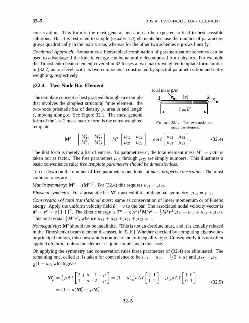
§32.4. Two-Node Bar Element

The template concept is best grasped through an examplethat involves the simplest structural finite element: thetwo-node prismatic bar of densityρ, areaA and length, moving alongx. See Figure 32.1. The most generalform of the 2× 2 mass matrix form is the entry-weightedtemplate

x1 2Total mass ρA

(e)

= Le

Figure 32.1. The two-node pris-matic bar element.

Me =[

Me11 Me

12Me

21 Me22

]= Me

[µ11 µ12

µ21 µ22

]= ρ A

[µ11 µ12

µ21 µ22

]. (32.4)

The first form is merely a list of entries. To parametrize it, the total element massMe = ρ A istaken out as factor. The free parametersµ11 throughµ22 are simply numbers. This illustrates abasic convenience rule:free template parameters should be dimensionless.

To cut down on the number of free parameters one looks atmass property constraints. The mostcommon ones are

Matrix symmetry: Me = (Me)T . For (32.4) this requiresµ21 = µ12.

Physical symmetry: For a prismatic barMe must exhibit antidiagonal symmetry:µ22 = µ11.

Conservation of total translational mass: same as conservation of linear momentum or of kineticenergy. Apply the uniform velocity fieldu = v to the bar. The associated nodal velocity vector isue = ve = v [ 1 1]T . The kinetic energy isTe = 1

2(ve)T Meve = 12 Mev2(µ11 + µ12 + µ21 + µ22).

This must equal12 Mev2, whenceµ11 + µ12 + µ21 + µ22 = 1.

Nonnegativity: Me should not be indefinite. [This is not an absolute must, and it is actually relaxedin the Timoshenko beam element discussed in 32.6.] Whether checked by computing eigenvaluesor principal minors, this constraint is nonlinear and of inequality type. Consequently it is not oftenappliedab initio, unless the element is quite simple, as in this case.

On applying the symmetry and conservation rules three parameters of (32.4) are eliminated. Theremaining one, calledµ, is taken for convenience to beµ11 = µ22 = 1

6(2 + µ) andµ12 = µ21 =16(1 − µ), which gives

Meµ = 1

6ρ A

[2 + µ 1 − µ

1 − µ 2 + µ

]= (1 − µ) 1

6ρ A

[2 11 2

]+ µ 1

2ρ A

[1 00 1

]= (1 − µ)Me

C + µMeL .

(32.5)

32–5


Expression (32.5) shows that the one-parameter template can be presented as a linear combinationof the well known consistent and diagonally-lumped mass matrices. So starting with the generalentry-weighted form (32.4) we end up with a two-matrix-weighted form befitting (32.2). Ifµ = 0andµ = 1, (32.5) reduces toMe

C andMeL respectively. This illustrates another desirable property:

the CMM and DLMM models ought to be instances of the template.

Finally we can apply the nonnegativity constraint. For the two principal minors ofMeµ to be

nonnegative, 2+ µ ≥ 0 and(2 + µ)2 − (1 − µ)2 = 3 + 6µ ≥ 0. Both are satisfied ifµ ≥ −/.Unlike the others, this constraint is of inequality type, and only limits the range ofµ.

The remaining task is to findµ. This is done by introducing anoptimality criterion that fits theproblem at hand. This is where customization comes in. Even for this simple case the answer is notunique. Thus the sentence “the best mass matrix for the two-node bar is so-and-so” has no uniquemeaning. Two specific optimization criteria are studied below.

§32.4.1. Best µ by Angular Momentum Preservation

Allow the bar to move in thex, y plane by expanding its nodal DOF toue = [ ux1 uy1 ux2 uy2 ]T

so (32.5) becomes a 4× 4 matrix

Meµ = 1

6ρ A

2 + µ 0 1− µ 00 2+ µ 0 1− µ

1 − µ 0 2+ µ 00 1− µ 0 2+ µ

(32.6)

Apply a uniform angular velocityθ about the midpoint. The associated node velocity vector atθ = 0 is ue = 1

2θ [ 0 −1 0 1]T . The discrete and continuum energies are

Teµ = 1

2(ue)T Meµue = 1

24ρ A3(1 + 2µ), Te =∫ /2

−/2ρ A

(θ x

)2dx = 1

24ρ A3. (32.7)

MatchingTeµ = Te givesµ = 0. So according to this criterion the optimal mass matrix is the

consistent one (CMM). Note that ifµ = 1, Teµ = 3Te, whence the DLMM overestimates the

rotational (rotary) inertia by a factor or 3.

§32.4.2. Best µ by Fourier Analysis

Another useful optimization criterion is the fidelitywith which planes waves are propagated over a barelement lattice, when compared to the case of a con-tinuum bar pictured in Figure 32.2.

Symbols used for propagation of harmonic waves arecollected in Table 32.1 for the reader’s convenience.(Several of these are reused in Sections 5 and 6.)The discrete counterpart of Figure 32.2 is shown inFigure 32.3.

ρ,E,A = const

x

u (x,t)

λ

Phase velocity c0

0

0

Figure 32.2. Propagation of a harmonic waveover an infinite, continuum prismatic bar. Thewave-profile axial displacementu(x, t) is plotted

normal to the bar.

This is a lattice of repeating two-node bar elements of length. Lattice wave propagation nomen-clature is similar to that defined for the continuum case in Table 32.1, but without zero subscripts.

32–6


Table 32.1 Nomenclature for Harmonic Wave Propagation in a Continuum Bar

Quantity Meaning(physical dimension in brackets)

ρ, E, A Mass density, elastic modulus, and cross section area of barρu0 = Eu′′

0 Bar wave equation. Alternate forms:−ω20u = c2

0u′′ and u′′ + k20u = 0.

u0(x, t) Waveformu0 = B0 exp(i (k0x − ω0t)

)[length], in which i = √−1

B0 Wave amplitude [length]λ0 Wavelength [length]k0 Wavenumberk0 = 2π/λ0 [1/length]ω0 Circular (a.k.a. angular) frequencyω0 = k0c0 = 2π f0 = 2πc0/λ0 [radians/time]f0 Cyclic frequencyf0 = ω0/(2π) [cycles/time: Hz if time in seconds]T0 PeriodT0 = 1/ f0 = 2π/ω0 = λ0/c0 [time]c0 Phase velocityc0 = ω0/k0 = λ0/T0 = λ0 f0 = √

E/ρ [length/time]κ0 Dimensionless wavenumberκ0 = k0λ0 (κ0 = 2π in continuum)0 Dimensionless circular frequency0 = ω0T0 = ω0λ0/c0

Zero subscripted quantities, such ask0 or c0, refer to the continuum bar. Unsubscriptedcounterparts, such ask or c, pertain to a discrete FEM lattice as in Figure 32.3.

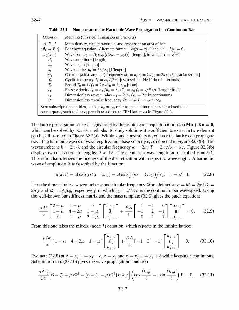
The lattice propagation process is governed by the semidiscrete equation of motionMu + Ku = 0,which can be solved by Fourier methods. To study solutions it is sufficient to extract a two-elementpatch as illustrated in Figure 32.3(a). Within some constraints noted later the lattice can propagatetravelling harmonic waves of wavelengthλ and phase velocityc, as depicted in Figure 32.3(b). Thewavenumber isk = 2π/λ and the circular frequencyω = 2π/T = 2πc/λ = kc. Figure 32.3(b)displays two characteristic lengths:λ and. The element-to-wavelength ratio is calledχ = /λ.This ratio characterizes the fineness of the discretization with respect to wavelength. A harmonicwave of amplitudeB is described by the function

u(x, t) = B exp[i (kx − ωt)] = B exp[i(κx − c0t

)/], i = √−1. (32.8)

Here the dimensionless wavenumberκ and circular frequency are defined asκ = k = 2π/λ =2πχ and = ω/c0, respectively, in whichc0 = √

E/ρ is the continuum bar wavespeed. Usingthe well-known bar stiffness matrix and the mass template (32.5) gives the patch equations

ρ A

6

[ 2 + µ 1 − µ 01 − µ 4 + 2µ 1 − µ

0 1− µ 2 + µ

] [ u j −1

u j

u j +1

]+ E A

[ 1 −1 0−1 2 −1

0 −1 1

] [ u j −1

u j

u j +1

]= 0. (32.9)

From this one takes the middle (nodej ) equation, which repeats in the infinite lattice:

ρ A

6[ 1 − µ 4 + 2µ 1 − µ ]

[ u j −1

u j

u j +1

]+ E A

[ −1 2 −1]

[ u j −1

u j

u j +1

]= 0. (32.10)

Evaluate (32.8) atx = xj −1 = xj − , x = xj andx = xj +1 = xj + while keepingt continuous.Substitution into (32.10) gives the wave propagation condition

ρ Ac20

3

[6 − (2 + µ)2 − (

6 − (1 − µ)2)

cosκ] (

cosc0t

− i sin

c0t

)B = 0. (32.11)

32–7


j

j

j

j−1

j−1

j+1

j+1x −j

x +j

Two-elementpatch

ρ,E,A = const

x uj

x j

(b)(a)

λ

Phase velocity c

Figure 32.3. An infinite lattice of two-node prismatic bar elements: (a) 2-elementpatch extracted from lattice; (b) characteristic dimensions for a propagating harmonic

wave.

If this is to vanish for anyt and B, the expression in brackets must vanish. Solving gives thefrequency-wavenumber relations

2 = 6(1 − cosκ)

2 + µ + (1 − µ) cosκ= κ2 + 1 − 2µ

12κ4 + 1 − 10µ + 10µ2

360κ6 + . . . ,

κ = arccos

[6 − (2 + µ)2

6 + (1 − µ)2

]= − 1 − 2µ

243 + 9 − 20µ + 20µ2

19205 + . . .

(32.12)

Returning to physical wavenumberk = κ/ and frequencyω = c0/:

ω2 =(

6c20

2

)1 − cos(k)

2 + µ + (1 − µ) cos(k)= c2

0k2

(1 + 1−2µ

12k22 + 1−10µ+10µ2

360k44 + . . .

)(32.13)

An equation that links frequency and wavenumber:ω = ω(k) as in (32.13), is adispersion relation.An oscillatory dynamical system isnondispersiveif ω is linear ink, in which casec = ω/k isconstant and the wavespeed is the same for all frequencies. The dispersion relation for the continuumbar (within the limits of MoM assumptions) isc0 = ω0/k0: all waves propagate with the samespeedc0. On the other hand the FEM model isdispersivefor anyµ, since from (32.12) we get

c

c0= ω

k c0= 1

κ

√6(1 − cosκ)

2 + µ + (1 − µ) cosκ= 1 + 1 − 2µ

24κ2 + 1 − 20µ + 20µ2

1920κ4 + . . . (32.14)

The best fit to the continuum forsmall wavenumbersκ = k<<1 is obtained by takingµ = /.This makes the second term of the foregoing series vanish. So from this standpoint the best massmatrix for the bar is

Meµ

∣∣µ=/

= 12Me

C + 12Me

L = ρ A

12

[5 11 5

]. (32.15)

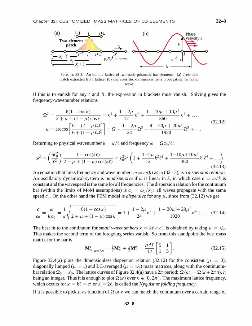
Figure 32.4(a) plots the dimensionless dispersion relation (32.12) for the consistent (µ = 0),diagonally lumped (µ = 1) and LC-averaged (µ = /) mass matrices, along with the continuum-bar relation0 = κ0. The lattice curves of Figure 32.4(a) have a 2π period:(κ) = (κ+2πn), nbeing an integer. Thus it is enough to plot(κ) overκ ∈ [0, 2π ]. The maximum lattice frequency,which occurs forκ = k = π or λ = 2, is called theNyquistor folding frequency.

If it is possible to pickµ as function of or κ we can match the continuum over a certain range of

32–8


0 1 2 3 4 5 6

1

2

3

4

5

6

Diagonally lumped mass: µ = 1

Consistent mass: µ = 0

Exact (Continuum Bar)

Dimensionless wavenumber κ=k Dimensionless wavenumber κ=k0 1 2 3 4 5 6

−0.4

−0.2

0

0.2

0.4

0.6

0.8

1

µM

µ = 1/2

LC averaged: µ = 1/2

(a) (b)D

imen

sion

less

freq

uenc

y

Ω=ω

/c

0

Figure 32.4. Results from Fourier analysis of two-node bar lattice: (a) dispersion curves forvarious choices ofµ; (b) wavenumber dependentµM that makes lattice match the continuum.

κ or . This can be done by equating = κ (or c = c0) and solving forµ:

µM = 1 + 6

κ2− 3

1− cosκ= 1

2− κ2

40− κ4

1008− κ6

28800− . . . = 1

2− 4π2χ2

40− 16π4χ4

1008− . . .

= 1 + 6

2− 3

1− cos= 1

2− 2

40− 4

1008− 6

28800− . . .

(32.16)in whichχ = 2π κ. The functionµM(κ) is plotted in Figure 32.4(b). Interesting values areµM = 0if κ = 3.38742306673364 andµM = −/ if κ = κlim = 4.05751567622863. Ifκ > κlim thefitted Me becomes indefinite. So (32.16) is practically limited to the range 0≤ k ≤≈ 4/ shownin the plot.

§32.4.3. *Best µ By Modified Equation

The gist of Fourier analysis is to find an exact solution, which separates space and time in the characteristicequation (32.11). The rest is routine mathematics. The method of modified differential equations or MoDE,introduced in §13.8, makes less initial assumptions but is not by any means routine. The objective is to finda MoDE that, if solved exactly, produces the FEM solution at nodes, and to compare it with the continuumwave equation given in Table 32.1. The method assumes only1 thatu = −ω2u, whereω is a lattice frequencyleft to be determined. This takes care of the time variation. Applying this assumption to the patch equation(32.10) and passing to dimensionless variables we get

[ −1 − 16(1 − µ)2 2 − 1

6(4 + 2µ)2 −1 − 16(1 − µ)2 ]

[u j −1

u j

u j +1

]= 0. (32.17)

1 This assumption is necessary because no discretization in the time domain has been specified. If a time integrator hadbeen applied, we would face a partial differential equation in space and time. That is a tougher nut to crack in anintroductory course.

32–9


in which = ω/c0 is the dimensionless circular frequency used in the previous subsection. This differenceequation is “continuified” by replacingu j → u(t) andu j ±1 → u(t ± ), and scaled through to produce thefollowing difference-differential form or DDMoDE:

[ − 12 ψ − 1

2 ]

[u(t − )

u(t)u(t + )

]= ψu(t) − 1

2

(u(t − ) + u(t + )

) = 0, with ψ = 6 − (2 + µ)2

6 + (1 − µ)2. (32.18)

As MoDE expansion coefficient we select the element-to-wavelength ratioχ = /λ. Accordingly, expandingthe the end values in Taylor series aboutu(t) givesu(t − ) = u j − u′(t) + 2u′′(t)/2! − . . ., andu(t + ) =u j + u′(t) + 2u′′(t)/2! + . . .. The foregoing semisum is12

(u(t − ) + u(t + )

) = u(t) + 2u′′(t)/2! +4u′′′′(t)/4! + . . ., which contains only evenu derivatives. Replacing into (32.18) and setting = λχ , weobtain the infinite-order modified differential equation or IOMoDE:

(1 − ψ)u + 1

2!λ2χ2u′′ + λ4χ4

4!u′′′′ + . . . = 0. (32.19)

This form needs further work. To see why, consider a mesh refinement process that makesχ → 0 while keepingλ fixed. Then (32.19) approaches(1 − ψ)u = 0. Sinceu = 0, ψ → 1 in the sense that 1− ψ = O(χ2). Toobtain the canonical MoDE form exhibited below, the transformation 1−ψ → 1

2γχ2, whereγ is another freecoefficient, is specified, and solved for2, giving2 = 6γχ2/(6− γ (1− µ)χ2). Replacing into (32.19)anddividing through by2 = λ2χ2 yields

γ

2λ2u + 1

2!u′′ + λ2χ2

4!u′′′′ + λ4χ4

6!u′′′′′′ + . . . = 0. (32.20)

This has the correct IOMoDE form: asχ− > 0 two terms survive and a second-order ODE emerges. In fact,but for the sign of the first term this is a canonical IOMoDE form studied in [62] for a different application. Thelast and quite complicated MoDE step is elimination of derivatives of order higher than two. The techniqueof that reference leads to the finite order modified equation or FOMoDE:

u′′ + 4

λ2χ2

(arcsin

χ√

γ

2

)2

u = 0. (32.21)

This is matched to the continuum bar equationu′′ + k20u = 0 of Table 32.1, assuming thatλ = λ0. Equating

coefficients givesk0λ0χ/2 = πχ = arcsin( 12χ

√γ ) or sin(πχ) = 1

2χ√

γ , whenceγ = 4 sin2(πχ)/χ2 and

2 = 6γχ2

6 − γ (1 − µ)χ2= 12 sin2(πχ)

2 + µ + (1 − µ) cos(2πχ)= 4π2χ2. (32.22)

The last equation comes from the definition = ω/c0 = 2πχ . Solving forµ gives the discrete-to-continuummatching value

µM = 1 + 3

2π2χ2− 3

2 cos2(πχ)= 1

2− π2χ2

10− π4χ4

63− π6χ6

450− . . . (32.23)

Replacing 2πχ by κ (or by = κ) givesµM = 1+6/κ2 −3/(1−cosκ), thus reproducing the result (32.16).So Fourier analysis and MoDE deliver the same result.

Remark 32.1. When Fourier can be used, as here, it is far simpler than MoDE. However the latter providesa side bonus:a priori error estimates. For example, suppose that one plans to put 10 elements within theshortest wavelength of interest. Thusχ = /λ = 1/10 andγ = 4 sin2(πχ)/χ2 = 38.1966. Replacing into(32.22) gives/(2πχ) = 1.016520, 0.999670 and 0.983632 forµ = 0, µ = / andµ = 1, respectively.The estimate frequency errors with respect to the continuum are 1.65%,−0.04% and−1.64%, respectively.

32–10

32–11 §32.5 THREE-NODE BAR ELEMENT

§32.5. Three-Node Bar Element

As pictured in Figure 32.5, this element is prismaticwith length , cross section areaA and mass densityρ. Midnode 3 is at the center. The element DOFs arearranged asue = [ u1 u2 u3 ]T . Its well known stiffnessmatrix is paired with a entry-weighted mass template:

x1 23

Total mass ρA

(e)

= Le

Figure 32.5. The three-node pris-matic bar element.

Ke = E A

3

[ 7 1 −81 7 −8

−8 −8 16

], Me

µ = ρ A

90

[ 12+ µ1 −3 + µ3 6 + µ4

−3 + µ3 12+ µ1 6 + µ4

6 + µ4 6 + µ4 48+ µ2

](32.24)

The idea behind the assumed form ofMeµ in (32.24) is to define the mass template as a parametrized

deviation from the consistent mass matrix. That is, settingµ1 = µ2 = µ3 = µ4 = 0 makesMe

µ = MeC. Settingµ1 = µ3 = 3,µ2 = 12 andµ4 = −6 gives the well known diagonally lumped

mass matrix (DLMM) generated by Simpson’s integration rule:MeL = ρ A diag

[/, /, /

].

Thus again the standard models are template instances. Notice thatMeν in (32.24) incorporates

matrix and physical symmetriesa priori but not conservation conditions.

Linear and angular momentum conservation requires 2µ1 + µ2 + 2µ3 + 4µ4 = 0 andµ3 = µ1,respectively. Eliminatingµ3 andµ4 from those constraints reduces the template to two parameters:

Meµ = ρ A

360

[ 4(12+ µ1) 4(−3 + µ1) 24− 4µ1 − µ2

4(−3 + µ1) 4(12+ µ1) 24− 4µ1 − µ2

24− 4µ1 − µ2 24− 4µ1 − µ2 4(48+ µ2)

](32.25)

For (32.25) to be nonnegative,µ1 ≥ −9/2 and 15+ µ1 − 3√

5√

9 + 2µ1 ≤ 14µ2 ≤ 15+ µ1 +

3√

5√

9 + 2µ1. These inequality constraints should be checkeda posteriori.

j

j

j−1j−2 j+1 j+2

x −j

x +j

Two-elementpatch

ρ,E,A = const

x

x j

Figure 32.6. Lattice of three-node bar elements from which a 2-element patch isextracted. Yellow and red-filled circles flag endnodes and midnodes, respectively.

32–11


§32.5.1. Patch Equations

Unlike the two-node bar, two free parameters remain after the angular momentum conservationcondition is enforced. Consequently we can ask for satisfactory wave propagation conditions inaddition to conservation. To assess performance of mass-stiffness combinations we carry out theplane wave analysis of the infinite beam lattice shown in Figure 32.6.

From the lattice we extract a typical two node patch as illustrated. The patch has five nodes: threeendpoints and two midpoints, which are assigned global numbersj −2, j −1, . . . j +2. The unforcedsemidiscrete dynamical equations of the patch areMP uP + KP uP = 0, where

MP = ρ A

360

4(12+ µ1) 24− 4µ1 − µ2 4(−3 + µ1) 0 0

24− 4µ1 − µ2 4(48+ µ2) 24− 4µ1 − µ2 0 04(−3 + µ1) 24− 4µ1 − µ2 8(12+ µ1) 24− 4µ1 − µ2 4(−3 + µ1)

0 0 24− 4µ1 − µ2 4(48+ µ2) 24− 4µ1 − µ2

0 0 4(−3 + µ1) 24− 4µ1 − µ2 4(12+ µ1)

KP = E A

3

7 −8 1 0 0

−8 16 −8 0 01 −8 14 −8 10 0 −8 16 −80 0 1 −8 7

, uP = [ u j −2 u j −1 u j u j +1 u j +2 ]T .

(32.26)

From the foregoing we keep the third and fourth equations, namely those for nodesj and j +1.This selection provides the equations for a typical corner pointj and a typical midpointj +1. Theretained patch equations are

MPj, j +1uP + KP

j, j +1uP = 0. (32.27)

The 2× 5 matricesMPj, j +1 andKP

j, j +1 result on deleting rows 1,2,5 ofMP andKP, respectively.

§32.5.2. Fourier Analysis

We study the propagation of harmonic plane waves of wavelengthλ, wavenumberk = 2π/λ, andcircular frequencyω over the lattice of Figure 32.6. For convenience they are separated into cornerand midpoint waves:

uc(x, t) = Bc ei (kx−ωt), um(x, t) = Bmei (kx−ωt). (32.28)

Waveuc(x, t) propagates only over corners and vanishes at midpoints, whereasum(x, t) propagatesonly over midpoints and vanishes at corners. Both have the same wavenumber and frequency butdifferent amplitudes and phases. [Waves (32.28) can be combined to form a single waveform thatpropagates over all nodes. The combination has two components that propagate with the samespeed but in opposite directions. This is useful when studying boundary conditions or transitionsin finite lattices, but is not needed for a periodic infinite lattice.] As in the two-node bar case, wewill work with the dimensionless frequency = ω/c0 and dimensionless wavenumberκ = k.

32–12


Inserting (32.28) into (32.26), passing to dimensionless variables and requiring that solutions existfor anyt yields the characteristic equation

1

180

[960− 2(48+ µ2)

2 −(960+ (24− 4µ1 − µ2)

2)

cos12κ

symm 4(210− (12+µ1)

2 + (30+ (3−µ1)2) cosκ

) ] [Bc

Bm

]= 0.

(32.29)For nontrivial solutions the determinant of the characteristic matrix must vanish. Solving for2

gives two frequencies for each wavenumberκ. They can be expressed as the dispersion relations

2a = φ1 + δ

φ5 + φ6 cosκ, 2

o = φ1 − δ

φ5 + φ6 cosκ, (32.30)

in which φ1 = 720(−208− µ2 + (µ2 − 32) cosκ), φ2 = 64(µ1 − 60)µ1 − 32µ1µ2 + 13µ22 +

384(474+µ2), φ3 = 12(−112+µ2)(128+µ2), φ4 = 64(132+(µ1−60)µ1)−32(µ1−6)µ2+µ22,

φ5 = 16(−540+ (µ1 − 60)µ1)− 8(30+µ1)µ2 +µ22, φ6 = 2880+ 16(µ1 − 60)µ1 − 8µ1µ2 +µ2

2

and δ = 120√

6√

φ2 − φ3 cosκ − φ4 cos 2κ. Frequenciesa and o pertain to the so-calledacousticandoptical branches, respectively. This nomenclature originated in crystal physics, inwhich both branches have physical meaning as modeling molecular oscillations. [In molecularcrystallography, acoustic waves are long-wavelength, low-frequency mechanical waves caused bysonic-like disturbances, in which adjacent molecules move in the same direction. Optical waves areshort-wavelength, high-frequency oscillations caused by interaction with light or electromagnetics,in which adjacent molecules move in opposite directions.Notes and Bibliography providesreferences.]

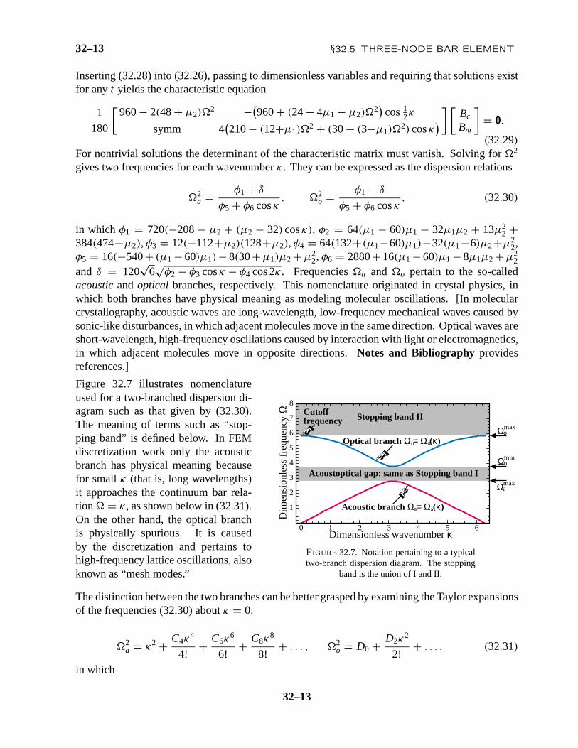
Figure 32.7 illustrates nomenclatureused for a two-branched dispersion di-agram such as that given by (32.30).The meaning of terms such as “stop-ping band” is defined below. In FEMdiscretization work only the acousticbranch has physical meaning becausefor smallκ (that is, long wavelengths)it approaches the continuum bar rela-tion = κ, as shown below in (32.31).On the other hand, the optical branchis physically spurious. It is causedby the discretization and pertains tohigh-frequency lattice oscillations, alsoknown as “mesh modes.”

Dimensionless wavenumber κ

Dim

ensi

onle

ss fr

eque

ncy Ω

0 1 2 3 4 5 6

1

2

3

4

5

6

7

8

Stopping band IICutoff frequency

Acoustoptical gap: same as Stopping band I

Ωomax

Ωamax

Ωomin

Optical branch Ω = Ω (κ)o o

Acoustic branch Ω = Ω (κ)aa

Figure 32.7. Notation pertaining to a typicaltwo-branch dispersion diagram. The stopping

band is the union of I and II.

The distinction between the two branches can be better grasped by examining the Taylor expansionsof the frequencies (32.30) aboutκ = 0:

2a = κ2 + C4κ

4

4!+ C6κ

6

6!+ C8κ

8

8!+ . . . , 2

o = D0 + D2κ2

2!+ . . . , (32.31)

in which

32–13


5 × 1440C4 = 14400− ψ21 = (240− 4µ1 + µ2)(4µ1 − µ2),

10× 14402 C6 = 41472000+ 7200ψ21 + 180ψ3

1 + ψ41 − 720ψ2

1ψ2,

60× 14403 C8 = −2030469120000+ 348364800ψ21 − 14515200ψ3

1 − 342720ψ41 − 2520ψ5

1

− 7ψ61 + 58060800ψ2

1ψ2 + 1451520ψ31ψ2 + 10080ψ4

1ψ2 − 2903040ψ21ψ2

2 ,

D0 = 1

ψ3, D2 = −ψ2

1(43200+ 360ψ1 + ψ21 − 1440ψ2)

ψ23

.

(32.32)

Here ψ1 = 4µ1 − µ2 − 120, ψ2 = µ1 − 2 andψ3 = 28800+ 360ψ1 + ψ21 − 1440ψ2 =

−2880− 960µ1 + 16µ21 − 120µ2 − 8µ1µ2 + µ2

2. Note that the expansion of2a approachesκ2

asκ → 0. Clearly the acoustic branch is the long-wavelength counterpart of the continuum bar,for which = κ. On the other hand, the optical branch has a nonzero frequency2

o = 1/ψ3 atκ = 0, called thecutoff frequency, which cannot vanish although it may go to infinity ifψ3 = 0. Asillustrated in Figure 32.7, the lowest and highest values ofo (taking the + square root of2

o) arecalledmax

o andmino , respectively, while the largesta is calledmax

a . Usually, but not always,min

0 andmaxa occur atκ = π .

If mino > max

a , the rangemino > > max

a is called theacoustoptical frequency gapor simplythe AO gap. Frequencies in this gap are said to pertain to portion I of thestopping band, a termderived from filter technology. Frequencies > max

o pertain to portion II of the stopping band.A stopping band frequency cannot be propagated as harmonic plane wave over the lattice. This canbe proven by showing that if pertains to the stopping band, the characteristic equation (32.29)has complex roots with nonzero real parts. This causes exponential attenuation so any disturbancewith that frequency will decay exponentially.

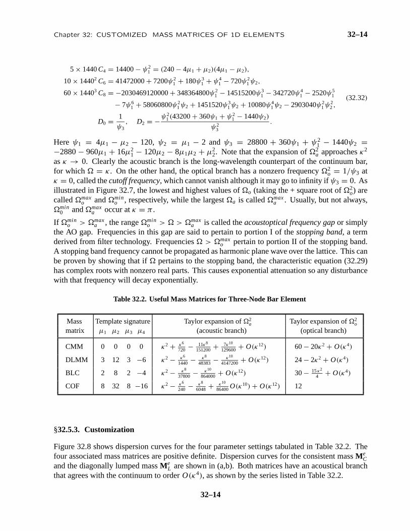
Table 32.2. Useful Mass Matrices for Three-Node Bar Element

Mass Template signature Taylor expansion of2a Taylor expansion of2

o

matrix µ1 µ2 µ3 µ4 (acoustic branch) (optical branch)

CMM 0 0 0 0 κ2 + κ6

720 − 11κ8

151200 + 7κ10

129600 + O(κ12) 60− 20κ2 + O(κ4)

DLMM 3 12 3 −6 κ2 − κ6

1440 − κ8

48383 − κ10

4147200+ O(κ12) 24− 2κ2 + O(κ4)

BLC 2 8 2 −4 κ2 − κ8

37800 − κ10

864000 + O(κ12) 30− 15κ2

4 + O(κ4)

COF 8 32 8 −16 κ2 − κ6

240 − κ8

6048 + κ10

86400O(κ10) + O(κ12) 12

§32.5.3. Customization

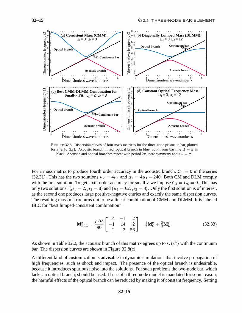
Figure 32.8 shows dispersion curves for the four parameter settings tabulated in Table 32.2. Thefour associated mass matrices are positive definite. Dispersion curves for the consistent massMe

Cand the diagonally lumped massMe

L are shown in (a,b). Both matrices have an acoustical branchthat agrees with the continuum to orderO(κ4), as shown by the series listed in Table 32.2.

32–14


Optical branchOptical branch

Optical branchOptical branch

Continuum bar

Continuum bar

Continuum bar

Acoustic branch Acoustic branch

Acoustic branchAcoustic branch

Dimensionless wavenumber κDimensionless wavenumber κ

Dimensionless wavenumber κ Dimensionless wavenumber κ

Dim

ensi

onle

ss fr

eque

ncy Ω

Dim

ensi

onle

ss fr

eque

ncy Ω

Dim

ensi

onle

ss fr

eque

ncy Ω

Dim

ensi

onle

ss fr

eque

ncy Ω

1 2

(c) Best CMM-DLMM Combination for Small-κ Fit: µ = 2, µ = 8

1 2

(a) Consistent Mass (CMM): µ = 0, µ = 0 1 2

(b) Diagonally Lumped Mass (DLMM): µ = 3, µ = 12

1 2

(d) Constant Optical Frequency Mass: µ = 3, µ = 12

0 1 2 3 4 5 6

1

2

3

4

5

6

7

8

0 1 2 3 4 5 6

1

2

3

4

5

6

7

8

0 1 2 3 4 5 6

1

2

3

4

5

6

7

8

0 1 2 3 4 5 6

1

2

3

4

5

6

7

8

Continuum bar

Figure 32.8. Dispersion curves of four mass matrices for the three-node prismatic bar, plottedfor κ ∈ [0, 2π ]. Acoustic branch in red, optical branch in blue, continuum bar line = κ in

black. Acoustic and optical branches repeat with period 2π ; note symmetry aboutκ = π .

For a mass matrix to produce fourth order accuracy in the acoustic branch,C4 = 0 in the series(32.31). This has the two solutionsµ2 = 4µ1 andµ2 = 4µ1 − 240. Both CM and DLM complywith the first solution. To get sixth order accuracy for smallκ we imposeC4 = C6 = 0. This hasonly two solutions:µ1 = 2, µ2 = 8 andµ1 = 62, µ2 = 8. Only the first solution is of interest,as the second one produces large positive-negative entries and exactly the same dispersion curves.The resulting mass matrix turns out to be a linear combination of CMM and DLMM. It is labeledBLC for “best lumped-consistent combination”:

MeBLC = ρ A

90

[ 14 −1 2−1 14 2

2 2 56

]= 1

3MeC + 2

3MeL . (32.33)

As shown in Table 32.2, the acoustic branch of this matrix agrees up toO(κ6) with the continuumbar. The dispersion curves are shown in Figure 32.8(c).

A different kind of customization is advisable in dynamic simulations that involve propagation ofhigh frequencies, such as shock and impact. The presence of the optical branch is undesirable,because it introduces spurious noise into the solutions. For such problems the two-node bar, whichlacks an optical branch, should be used. If use of a three-node model is mandated for some reason,the harmful effects of the optical branch can be reduced by making it of constant frequency. Setting

32–15


µ1 = 8, µ2 = 32 produces the mass

MeCOF = ρ A

90

[ 10 5 −105 10 −10

−10 −10 80

], (32.34)

in which acronym COF stands for “Constant Optical Frequency.” Then2o = 12 for all wavenum-

bers, as pictured in Figure 32.8(d). This configuration maximizes the stopping band and facilitatesthe implementation of a narrow band filter cented at that frequency. The acoustic branch accuracyis inferior to that of the other models, however, so this customization involves a tradeoff.

One final parameter choice is worth mentioning as a curiosity. Settingµ1 = −2, µ2 = −8produces a dispersion diagramwith no stopping band: the optical branch comes down from+∞at κ = 0, 2π and merges with the acoustic branch atκ = π . The application of this mass matrix(which is singular) as a modeling tool is presently unclear and its dispersion diagram is omitted.

§32.6. The Bernoulli-Euler Beam

The Bernoulli-Euler beam model is a special case of the Timoshenko beam treated in the nextsection. It is nonetheless useful to do its mass template first, since results provide a valuable crosscheck with the more complicated Timoshenko beam. We take the consistent mass matrix derivedin the previous chapter, and modify their entries to produce the following entry-weighted template:

Meµ = ρ A

1335 + µ11 ( 11

210 + µ12)970 + µ13 −( 13

420 + µ14)

( 1105 + µ22)

2 ( 13420 + µ23) −( 1

140 + µ24)2

1335 + µ11 −( 11

210 + µ12)

symm ( 1105 + µ22)

2

(32.35)

The parameters in (32.35) areµi j , wherei j identifies the mass matrix entry. The template (32.35)accounts for matrix symmetry and some physical symmetries. Three more conditions can beimposed right away:µ14 = µ23, µ13 = −µ11 and 2µ12 = µ11 + 2µ22 + 2µ23 − 2µ24. Thefirst comes from beam symmetry and the others from conservation of total translational mass andangular momentum, respectively. This reduces the free parameters to four:µ11, µ22, µ23, µ24.The Fourier analysis procedure should be familiar by now to the reader. An infinite lattice ofidentical beam elements of length is set up. Plane waves of wavenumberk and frequencyωpropagating over the lattice are represented by

v(x, t) = Bvexp(i (kx − ωt

), θ(x, t) = Bθexp

(i (kx − ωt

)(32.36)

At a typical lattice nodej there are two freedoms:v j andθ j . Two patch equations are extracted, andconverted to dimensioneless form on definingκ = k and = ωc0/, in whichc0 = E I/(ρ A4)

is a reference phase velocity. The condition for wave propagation gives the characteristic matrixequation

det

[Cvv Cvθ

Cθv Cθθ

]= CvvCθθ − CvθCθv = 0, (32.37)

32–16

32–17 §32.6 THE BERNOULLI-EULER BEAM

whereCvv = (840−2(13+35µ11)

2 − (840+(9−70µ11)2) cosκ

)/35,−Cθv = Cvθ = i

(2520+

(13+420µ23)2)

sinκ/210,Cθθ = (1680−4(1+105µ22)

2+(840+3(1+140µ24)2) cosκ

)/210.

The condition (32.37) gives a quadratic equation in2 that provides two dispersion solutions: acous-tical branch2

a(κ) and optical branch2o(κ). These were already encountered in the analysis of the

3-node bar in §32.2. The acoustical branch represent genuine flexural modes, whereas the opticalone is a spurious byproduct of the discretization. The small-κ (long wavelength) expansions ofthese roots are

2a = κ4 + C6κ

6 + C8κ8 + C10κ

10 + C12κ12 + . . . , 2

o = D0 + D2κ2 + D4κ

4 + . . . ,

(32.38)in whichC6 = −µ11 − 2µ22 − 4µ23 + 2µ24, C8 = 1/720+ µ2

11 + 4µ222 + 2µ23/3 + 16µ22µ23 +

16µ223 + µ11(1/12+ 4µ22 + 8µ23 − 4µ24) − µ24 − 8µ22µ24 − 16µ23µ24 + 4µ2

24, etc.; andD0 =2520/(1 + 420µ22 − 420µ24), etc.Mathematicacalculated these series up toC14 andD4.

The continuum dispersion curve is2 = κ4, which automatically matches2a asκ → 0. Thus

four free parameters offer the opportunity to match coefficients of four powers:κ6, κ8, κ10, κ12.But it will be seen that the last match is unfeasible ifMe is to stay nonnegative. We settle for ascheme that agrees up toκ10. SettingC6 = C8 = C10 = 0 while keepingµ22 free yields two setsof solutions, of which the useful one is

µ11 = 4µ22 − 67/540− (4/27)√

38/35− 108µ22,

µ23 = 43/1080− 2µ22 +√

95/14− 675µ22/54,

µ24 = 19/1080− µ22 +√

19/70− 27µ22/27.

(32.39)

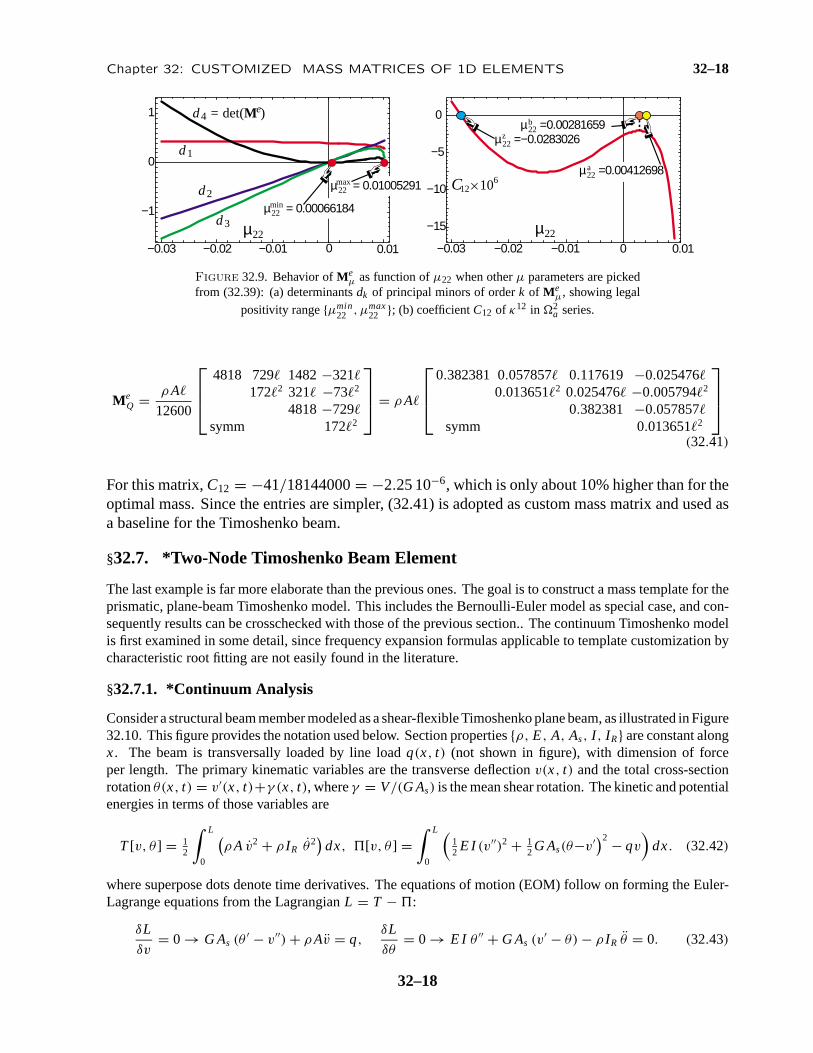
The positivity behavior ofMeµ asµ22 is varied is shown in Figure 32.9(a).M(e) is indefinite for

µ22 < µmin22 = (27−4

√35)/5040= 0.0006618414419844316. At the other extreme the solutions

of (32.39) become complex ifµ22 > µmax22 = 19/1890= 0.010052910052910053.

Figure 32.9(b) plotsC12(µ22) = (−111545− 3008ψ + 15120(525+ 4ψ)µ22)/685843200, withψ = √

70√

19− 1890µ22. This has one real rootµz22 = −0.02830257472322391, but that

gives an indefinite mass matrix. Forµ22 in the legal range [µmin22 , µmax

22 ], C12 is minimized forµb

22 = (25√

105− 171)/30240= 0.0028165928951385567, which substituted gives the optimalmass matrix:

MeB = ρ A

30240

a11 1788 a13 −732a22

2 732 a242

a33 1788symm a44

2

= ρ A

0.389589 0.059127 0.110410 −0.0242060.0123402 0.024206 −0.0055482

0.389589 −0.0591270.0123402

(32.40)

in whicha11 = a33 = 12396− 60√

105,a13 = 2724+ 60√

105,a22 = a44 = 117+ 25√

105 anda24 = −219+ 5

√105. For this set,C12 = (25

√105− 441)/91445760= −2.02 10−6. Another

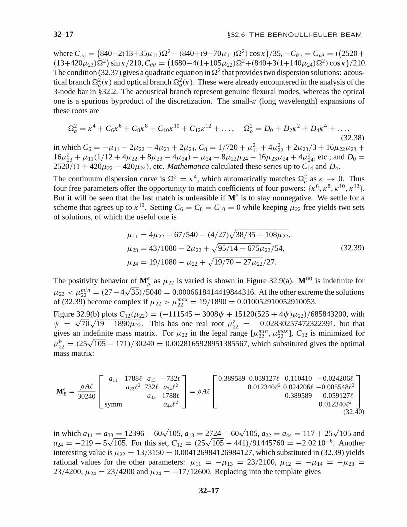
interesting value isµ22 = 13/3150= 0.004126984126984127, which substituted in (32.39) yieldsrational values for the other parameters:µ11 = −µ13 = 23/2100, µ12 = −µ14 = −µ23 =23/4200,µ24 = 23/4200 andµ24 = −17/12600. Replacing into the template gives

32–17


−0.03 −0.02 −0.01 0 0.01

−1

0

1

−0.03 −0.02 −0.01 0 0.01

−15

−10

−5

0

µ 22µ 22

126C ×10

d = det(M ) 4

d2

d3

d1

e

µ = 0.01005291 22max

µ = 0.00066184 22min

µ =−0.0283026 22z

µ =0.00281659 22b

µ =0.00412698 22a

Figure 32.9. Behavior ofMeµ as function ofµ22 when otherµ parameters are picked

from (32.39): (a) determinantsdk of principal minors of orderk of Meµ, showing legal

positivity rangeµmin22 , µmax

22 ; (b) coefficientC12 of κ12 in 2a series.

MeQ = ρ A

12600

4818 729 1482−3211722 321 −732

4818−729symm 1722

= ρ A

0.382381 0.057857 0.117619 −0.0254760.0136512 0.025476 −0.0057942

0.382381 −0.057857symm 0.0136512

(32.41)

For this matrix,C12 = −41/18144000= −2.25 10−6, which is only about 10% higher than for theoptimal mass. Since the entries are simpler, (32.41) is adopted as custom mass matrix and used asa baseline for the Timoshenko beam.

§32.7. *Two-Node Timoshenko Beam Element

The last example is far more elaborate than the previous ones. The goal is to construct a mass template for theprismatic, plane-beam Timoshenko model. This includes the Bernoulli-Euler model as special case, and con-sequently results can be crosschecked with those of the previous section.. The continuum Timoshenko modelis first examined in some detail, since frequency expansion formulas applicable to template customization bycharacteristic root fitting are not easily found in the literature.

§32.7.1. *Continuum Analysis

Consider a structural beam member modeled as a shear-flexible Timoshenko plane beam, as illustrated in Figure32.10. This figure provides the notation used below. Section propertiesρ, E, A, As, I , I R are constant alongx. The beam is transversally loaded by line loadq(x, t) (not shown in figure), with dimension of forceper length. The primary kinematic variables are the transverse deflectionv(x, t) and the total cross-sectionrotationθ(x, t) = v′(x, t)+γ (x, t), whereγ = V/(G As) is the mean shear rotation. The kinetic and potentialenergies in terms of those variables are

T [v, θ ] = 12

∫ L

0

(ρ A v2 + ρ I R θ2

)dx, [v, θ ] =

∫ L

0

(12 E I (v′′)2 + 1

2G As(θ−v′)2 − qv

)dx. (32.42)

where superpose dots denote time derivatives. The equations of motion (EOM) follow on forming the Euler-Lagrange equations from the LagrangianL = T − :

δL

δv= 0 → G As (θ ′ − v′′) + ρ Av = q,

δL

δθ= 0 → E I θ ′′ + G As (v′ − θ) − ρ I R θ = 0. (32.43)

32–18

32–19 §32.7 *TWO-NODE TIMOSHENKO BEAM ELEMENT

x, u

y, v

slope v' = dv/dx

Deformed cross

section

Normal todeformed

longitudinalaxis

v(x)

γ

L

Section-averagedshear rotation

+γ

+Vxz

y

V

M

A positive transverse shear force V = GA γ producesa CCW rotation (+γ) of the beam cross section

s

Positive bending moment and transverse shear conventions

ρ, E, G, A, A , I and I constant along beam

s R

Figure 32.10. A plane beam member modeled as Timoshenko beam, illustrating notationfollowed in the continuum analysis. Transverse loadq(x) not shown to reduce clutter.

Infinitesimal deflections and deformations grossly exaggerated for visibility.

An expedient way to eliminateθ is to rewrite the coupled equations (32.43) in transform space:[ρ As2 − G As p2 G As p

G As p E I p2 − G As − ρ I R s2

] [v

θ

]=

[q0

], (32.44)

in which p, s, v, θ , q denote transforms ofd/dx, d/dt, v, θ, q, respectively (Fourier inx and Laplace int). Eliminatingθ and returning to the physical domain yields

E I v′′′′ + ρ Av −(

ρ I R + ρ AE I

G As

)v′′ + ρ2 AIR

G As

....v = q − E I

G Asq′′ + ρ I R

G Asq. (32.45)

(Note that this derivation does not pre-assumeI ≡ I R, as usually done in textbooks.) For the unforced caseq = 0, (32.45) has plane wave solutionsv = B exp

(i (k0 x − ω0 t)

). The propagation condition yields a

characteristic equation relatingk0 andω0. To render it dimensionless, introduce a reference phase velocityc2

0 = E I/(ρ AL4) so thatk0 = ω0/c0 = 2π/λ0, a dimensionless frequency = ω0L/c0 and a dimensionlesswavenumberκ = k0L. As dimensionless measures of relative bending-to-shear rigidities and rotary inertiatake

0 = 12E I/(G AsL2), r 2R = I R/A, 0 = r R/L . (32.46)

The resulting dimensionless characteristic equation is

κ4 − 2 − ( 1120 + 2

0) κ2 2 + 1120 2

0 4 = 0. (32.47)

This is quadratic in2. Its solution yields two kinds of squared-frequencies, which will be denoted by2f

and2s because they are associated with flexural and shear modes, respectively. Their expressions are listed

below along with their small-κ (long wavelength) Taylor series:

2f = 6

P − √Q

020

= κ4 − ( 1120 + 2

0) κ6 + ( 1144

20 + 1

4020 + 4

0) κ8

− ( 11728

30 + 1

2420

20 + 1

2040 + 6

0) κ10 + . . . = A4κ4 + A6κ

6 + A8κ8 + . . .

(32.48)

2s = 6

P + √Q

020

= 12

020

+(

12

0+ 1

20

)κ2 − κ4 + ( 1

120 + 20)κ

6 + . . . = B0 + B2κ2 + . . . (32.49)

in which P = 1 + κ2(20 + 1

120) and Q = P2 − 13κ40

20. The dispersion relation2

f (κ) defines theflexural frequency branchwhereas2

s(κ) defines theshear frequency branch. If 0 → 0 and0 → 0, which

32–19


ν = 0 ν = 0

ν = 0

ν = 0

ν = 1/2

ν = 1/2

ν = 1/2

ν = 1/2

Bernoulli-Eulermodel

Bernoulli-Eulermodel

Dimensionless wavenumber κ Dimensionless wavenumber κ

Dim

ensi

onle

ss fr

eque

ncy Ω

Dim

ensi

onle

ss s

peed

Ω/κ

(a) (b)

0 5 10 15 20 25

50

100

150

200

250

300Shear branches ofTimoshenko model

Shear branches ofTimoshenko model

Flexural branches ofTimoshenko model Flexural branches of

Timoshenko model0 5 10 15 20 25

5

10

15

20

25

30

35

40

Cutoff frequencies

Figure 32.11. Spectral behavior of continuum Timoshenko beam model for a narrowb× h rectangular crosssection. (a): dispersion curves(κ) for = h/ = 1/4 and two Poisson’s ratios; Timoshenko flexural and

shear branches in red and blue, respectively; Bernoulli-Euler curve = κ2 in black. (b) Wavespeed/κ.

reduces the Timoshenko model to the Bernoulli-Euler one, (32.47) collapses to2 = κ4 or (in principalvalue) = κ2. This surviving branch pertains to flexural motions while the shear branch disappears — ormore precisely,2

s(κ) → +∞. It is easily shown that the radicandQ in the exact expressions is strictlypositive for any0 > 0, 0 > 0, κ ≥ 0. Thus for any such triple,2

f and2s are real, finite and distinct

with 2f (κ) < 2

s(κ); furthermore2f ,

2s increase indefinitely asκ → ∞. Following the nomenclature

introduced in Figure 32.7, the values atκ = 0 is called the cutoff frequency.

To see how branches look like, consider a beam of narrow rectangular cross section of widthb and heighth, fabricated of isotropic material with Poisson’s ratioν. We haveE/G = 2(1 + ν) and As/A ≈ 5/6.[Actually a more refinedAs/A ratio would be 10(1 + ν)/(12 + 11ν), but that makes little difference inthe results.] We haveA = bh, I = I R = bh3/12, r 2

R = I R/A = h2/12, 20 = r 2

R/L2 = 112h2/L2 and

0 = 12E I/(G AsL2) = 12(1 + ν)h2/(5L2). Since0/12 = 12(1 + ν) 20/5, the first-order effect of shear

on 2f , as measured by theκ6 term in (32.48), is 2.4 to 3.6 times that from rotary inertia, depending onν.

Replacing into (32.48) and (32.49) yields

2f

2s

=

60+ κ2(17+ 12ν)2 ∓√(

60+ κ2(17+ 12ν)2)2 − 240κ4(1 + ν)4

2(1 + ν)4

=

κ4 − 160(17+ 12ν)2 κ6 + 1

3600(349+ 468ν + 144ν2)4κ8 + . . .

60+ (17+ 12ν)2κ2 − (1 + ν)4 κ4 + . . .

(1 + ν)4

(32.50)

in which = h/L. Dispersion curves(κ) for = h/L = /andν = 0, /are plotted in Figure 32.11(a).Phase velocities/κ are shown in Figure 32.11(b). The figure also shows the flexural branch of the Bernoulli-Euler model. The phase velocities of the Timoshenko model tend to finite values in the shortwave, high-frequency limitκ → ∞, which is physically correct. The Bernoulli-Euler model is wrong in that limitbecause it predicts an infinite propagation speed.

32–20


§32.7.2. *Beam Element

The shear-flexible plane beam member of Figure 32.10is discretized by two-node elements. An individual ele-ment of this type is shown in Figure 32.12, which illus-trates its kinematics. The element has four nodal free-doms arranged as

ue = [ v1 θ1 v2 θ2 ]T (32.51)

Hereθ1 = v1 + γ1 andθ2 = v2 + γ2 are the total crosssection rotations evaluated at the end nodes.

θ1

x, u2

2

θ2

1γ

2γ

γ

1

y, v

1v11v' =[dv/dx]

22v' =[dv/dx]

vv(x)

Figure 32.12. Two-node element for Timo-shenko plane beam, illustrating kinematics.

The dimensionless properties (32.46) that characterize relative shear rigidity and rotary inertia are redefinedusing the element length:

= 12E I/(G As2), r 2

R = I R/A, = r R/. (32.52)

If the beam member is divided intoNe elements of equal length, = L/Ne whence = 0N2e and = 0Ne.

Thus even if0 and0 are small with respect to one, they can grow without bound as the mesh is refined.For example if0 = 1/4 and2

0 = 1/100, which are typical values for a moderately thick beam, and we takeNe = 32, then ≈ 250 and2 ≈ 10. Those are no longer small numbers, a fact that will impact performanceasNe increases. The stiffness matrix to be paired with the mass template is taken to be that of the equilibriumelement:

Ke = E I

3(1 + )

12 6 −12 66 2(4 + ) −6 2(2 − )

−12 −6 12 −6

6 2(2 − ) −6 2(4 + )

(32.53)

This is known to be nodally exact in static analysis for a prismatic beam member, and therefore an optimalchoice in that sense.

§32.7.3. *Setting Up the Mass Template

FEM derivations usually split the 4× 4 mass matrix of this element intoMe = Mev + Me

θ , whereMev andMe

θ

come from the translational inertia and rotary inertia terms, respectively, of the kinetic energy functionalT [v, θ ]of (32.42). The most general mass template would result from applying a entry-weighted parametrization ofthose two matrices. This would require a set of 20 parameters (10 in each matrix), reducible to 9 through11 on account of invariance and conservation conditions. Attacking the problem this way, however, leads tounwieldy algebraic equations even with the help of a computer algebra system, while concealing the underlyingphysics. A divide and conquer approach works better. This is briefly outlined next and covered in more detailin the next subsections.

(I) ExpressMe as the one-parameter matrix-weighted formMe = (1 − µ0) MeF + µ0 Me

D . HereMeF is full

and includes the CMM as instance, whereasMeD is 2× 2 block diagonal and includes the DLMM as instance.

This is plainly a generalization of the LC linear combination (32.2).

(II) Decompose the foregoing mass components asMeF = Me

FT +MF R andMeD = Me

DT +MeDR, where T and

R subscripts identify their source in the kinetic energy functional:T if coming from the translational inertiaterm 1

2ρ A v2 andR from the rotary inertia term12ρ I R θ2.

(III) Both components ofMeF are expressed as parametrized spectral forms, whereas those ofMe

D are expressedas entry-weighted. The main reasons for choosing spectral forms for the full matrix are reduction of parametersand physical transparency. No such concerns apply toMe

D .

The analysis follows a “bottom up” sequence, in order (III)-(II)-(I). This has the advantage that if a satisfactorycustom mass matrix for a target application emerges during (III), stages (II) and (I) need not be carried out,and that matrix directly used by setting the remaining parameters to zero.

32–21


§32.7.4. *Full Mass Parametrization

As noted above, one starts with full-matrix spectral forms. Letξ denote the natural coordinate that varies from−1 at node 1 to+1 at node 2. Two element transverse displacement expansions in generalized coordinatesare introduced:

vT (ξ) = L1(ξ) cT1 + L2(ξ) cT2 + L3(ξ) cT3 + L4(ξ) cT4 = LT cT ,

vR(ξ) = L1(ξ) cR1 + L2(ξ) cR2 + L3(ξ) cR3 + L4(ξ) cR4 = LR cR,

L1(ξ) = 1, L2(ξ) = ξ, L3(ξ) = 12(3ξ2 − 1), L4(ξ) = 1

2(5ξ3 − 3ξ),

L4(ξ) = 12

(5ξ3 − (5 + 10)ξ

) = L4(ξ) − (1 + 5)ξ.

(32.54)

ThevT andvR expansions are used for the translational and rotational parts of the kinetic energy, respectively.The interpolation function setLi used forvT is formed by the first four Legendre polynomials overξ =[−1, 1]. The set used forvR is the same except thatL4 is adjusted toL4 to produce a diagonal rotational massmatrix. All amplitudescT i andcRi have dimension of length.

Unlike the usual Hermite cubic shape functions, the polynomials in (32.54) have a direct physical interpretation.L1: translational rigid mode;L2: rotational rigid mode;L3: pure-bending mode symmetric aboutξ = 0; L4

andL4: bending-with-shear modes antisymmetric aboutξ = 0.

With the usual abbreviation(.)′ ≡ d(.)/dx = (2/)d(.)/dξ , the associated cross section rotations are

θT = v′T + γT = L′

T cT + γT , θR = v′R + γR = L′

R cR + γR, (32.55)

in which the mean shear distortions are constant over the element:

γT = 2

12v′′′

T = 10

cT4, γR = 2

12v′′′

R = 10

cR4. (32.56)

The kinetic energy of the element in generalized coordinates is

Te = 12

∫

0

(ρ A v2

T + ρ I R θ2R

)dx =

4

∫ 1

−1

(ρ A v2

T + ρ I R θ2R

)dξ = 1

2 cTT DT cT + 1

2 cTR DR cR, (32.57)

in which both generalized mass matrices turn out to be diagonal as intended:

DT = ρ A diag [ 1 13

15

17 ] , DR = 4ρ A2 diag [ 0 1 3 5] .

To convertDT andDR to physical coordinates (32.51),vT , vR, θT andθR are evaluated at the nodes by settingξ = ±1. This establishes the transformationsue = GT cT andue = GR cR. Inverting: cT = HT ue andcR = HR ue with HT = G−1

T andHR = G−1R . A symbolic calculation yields

HT = 1

60(1 + )

30(1 + ) 5(1 + ) 30(1 + ) −5(1 + )

−36− 30 −3 36+ 30 −3

0 −5(1 + ) 0 5(1 + )

6 3 −6 3

HR = 1

60(1 + )

30(1 + ) 5(1 + ) 30(1 + ) −5(1 + )

−30 15 30 150 −5(1 + ) 0 5(1 + )

6 3 −6 3

(32.58)

MatricesHT andHR differ only in the second row. This comes from the adjustment ofL4 to L4 in (32.54).To render this into a spectral template inject six free parameters in the generalized masses while moving 42

insideDRµ:

DTµ = ρ A diag [ 1 13µT1

15µT2

17µT3 ] , DRµ = ρ A diag [ 0 µR1 3µR2 5µR3 ] . (32.59)

32–22


The transformation matrices (32.58) are reused without change to produceMeF = HT

T DTµHT + HTRDRµHR.

If µT1 = µT2 = µT3 = 1 andµR1 = µR2 = µR3 = 42 one obtains the well known consistent mass matrix(CMM) of Archer, listed in [140, p. 296], as a valuable check. The configuration (32.59) already accounts forlinear momentum conservation, which is why the upper diagonal entries are not parametrized. Imposing alsoangular momentum conservation requiresµT1 = 1 andµR1 = 42, whence the template is reduced to fourparameters:

MeF = ρ A HT

T

1 0 0 00 1

3 0 00 0 1

5µT2 00 0 0 1

7µT3

HT + ρ A HTR

0 0 0 00 42 0 00 0 3µR2 00 0 0 5µR3

HR. (32.60)

Because bothHT andHR are nonsingular, choosing all four parameters in (32.60) to be nonnegative guaranteesthatMe

F is nonnegative. This useful property eliminates lengthya posteriorichecks.

SettingµT2 = µT3 = µR2 = µR3 = 0 and = 0 yields the correct mass matrix for a rigid beam, includingrotary inertia. This simple result highlights the physical transparency of spectral forms.

§32.7.5. *Block-Diagonal Mass Parametrization

Template (32.60) has a flaw: it does not include the DLMM. To remedy the omission, a block diagonal form,with four free parameters:νT1, νT2, νR1, νR2. is separately constructed:

MeD = MDT + MDR = ρ A

/ νT1 0 0νT1 νT2

2 0 00 0 / −νT1

0 0 −νT1 νT22

+ ρ A

0 νR1 0 0νR1 νR2

2 0 00 0 0 −νR1

0 0 −νR1 νR22

(32.61)

Four parameters can be merged into two by adding:

MeD = ρ A

/ ν1 0 0ν2 ν2

2 0 00 0 / −ν1

0 0 −ν1 ν22

. (32.62)

whereν1 = νT1 + νR1 andν2 = νT2 + νR2. Sometimes it is convenient to use the split form (32.61), forexample in lattices with varying beam properties or lengths, a topic not considered there. Otherwise (32.62)suffices. Ifν1 = 0, Me

D is diagonal. However for computational purposes a block diagonal form is just asgood and provides additional customization power. Terms in the (1,1) and (3,3) positions must be as shown tosatisfy linear momentum conservation. If angular momentum conservation is imposeda priori it is necessaryto setν2 = 1

22, and only one parameter remains.

The general template is obtained as a linear combination ofMeF andMe

D :

Me = (1 − µ0)MeF + µ0Me

D (32.63)

Summarizing there is a total of 7 parameters to play with: 4 inMeF , 2 in Me

D , plusµ0. This is less that the9-to-11 that would result from a full entry-weighted parametrization, so not all possible mass matrices areincluded by (32.63).

32–23


§32.7.6. *Fourier Analysis

An infinite lattice of identical beam elements of length is set up. Plane waves of wavenumberk and frequencyω propagating over the lattice are represented by

v(x, t) = Bvexp(i (kx − ωt

), θ(x, t) = Bθexp

(i (kx − ωt

)(32.64)

At each typical lattice nodej there are two freedoms:v j andθ j . Two patch equations are extracted, andconverted to dimensionless form on definingκ = k and = ωc/, in whichc = E I/(ρ A4) is a referencephase velocity. (Do not confuse withc0). The condition for wave propagation gives the characteristic matrixequation

det[

Cvv Cvθ

Cθv Cθθ

]= CvvCθθ − CvθCθv = 0, (32.65)

where the coefficients are complicated functions not listed there. Solving the equation provides two equations:2

a and2o, wherea ando denote acoustic and optical branch, respectively. These are expanded in powers of

κ for matching to the continuum. For the full mass matrix one obtains

2a = κ4 + C6κ

6 + C8κ8 + C10κ

10 + . . . , 2o = D0 + D2κ

2 + . . . (32.66)

Coefficients up toκ12 were computed byMathematica. Relevant ones for parameter selection are

C6 = −/12− 2,

C8 = [2 − 15µR2 − µT2 + 5(1 + ) + 60(1 + 3)2 + 7204

]/720,

C10 = [ − 44+ 35µT2 − 3µT3 − 282 + 525µR2(1 + ) − 105µR3(1 + )+1575µR2(1 + ) − (3µT3 − 35µT2(4 + 3) + 35(17+ 5(3 + )))+(−2940+ 12600µR2(1 + ) + 420(2µT2(1 + ) − 5(7 + 6(2 + ))))2−25200(2 + (7 + 6))4 − 302400(1 + )6

]/[302400(1 + )

],

D0 = 25200(1 + )/[7 + 105µR2 + 3µT3 + 210022

],

D2 = [2100(1 + )(−56− 35µT2 + 3µT3 − 63 + 3µT3 + 105µR3(1 + )−525µR2(1 + )2 − 35µT2(2 + )) + 2100(1 + )(3360 + 63002+21003)2 + 529200002(1 + )4

]/[7 + 105µR2 + 3µT3 + 210022

]2

(32.67)

For the block-diagonal template (32.62):

2a = κ4 + F6κ

6 + F8κ8 + F10κ

10 + . . . , 2o = G0 + G2κ

2 + . . . (32.68)

where

F6 = −24ν2 − , F8 = 2880ν2 − 5 + 360ν2 − 1 − 5 + 52

720

G0 = 6

ν2(1 + ), G2 = 24ν2 + − 2

2ν2(1 + )

(32.69)

The expansions for the 7-parameter template (32.63) are considerably more complicated than the above ones,and are omitted to save space.

32–24


Table 32.3. Useful Template Instances for Timoshenko Beam Element

Instance Description Commentsname

CMM Consistent mass matrix of Archer.Matches flexural branch up toO(κ6).

A popular choice. Fairly inaccurate, however,as beam gets thicker. Grossly overestimatesintermediate frequencies.

FBMS Flexural-branch matched toO(κ10)

with spectral (Legendre) template(32.60).

Converges faster than CMM. Performance de-grades as beam gets thicker, however, andelement becomes inferior to CDLA.

SBM0 Shear branch matched toO(κ0)whileflexure fitted toO(κ10)

Custom application: to roughly match shearbranch and cutoff frequency as mesh is refined.Danger: indefinite for certain ranges of and. Use with caution.

SBM2 Shear branch matched toO(κ2)whileflexure fitted toO(κ8)

Custom application: to finely match shearbranch and cutoff frequency as mesh is refined.Danger: indefinite for wide ranges of and.Use with extreme caution.

DLMM Diagonally lumped mass matrix withrotational mass picked to match flexuralbranch toO(κ6).

Obvious choice for explicit dynamics. Accu-racy degrades significantly, however, as beamgets thicker. Underestimates frequencies. Be-comes singular in the Bernoulli-Euler limit.

CDLA Average of CMMand DLMM.Matchesflexure branch toO(κ8).

Robust all-around choice. Less accurate thanFBMS and FBMG for thin beams, but becomestop performer as aspect ratio increases. Easilyconstructed if CMM and DLMM available incode.

FBMG Flexural branch matched toO(κ10)

with 7-parameter template (32.63).Known to be the globally optimal positive-definite choice for matching flexure in theBernoulli-Euler limit. Accuracy, however, isonly marginally better than FBMS. As in thecase of the latter, performance degrades as beamgets thicker.

§32.7.7. *Template Instances

Seven useful instances of the foregoing templates are identified and described in Table 32.3. Table 32.4 liststhe template signatures that generate those instances. These tables include two existing mass matrices (CMMand DLMM) re-expressed in the template context, and five new ones. The latter were primarily obtained bymatching series such as (32.67) and (32.68) to the continuum ones (32.48) and (32.49), up to a certain numberof terms as described in Table 32.3.

For the spectral template it is possible to match the flexure branch up toO(κ10). Trying to matchO(κ12) leadsto complex solutions. For the diagonal template the choice is more restrictive. It is only possible to matchflexure up toO(κ6), which leads to instance DLMM. Trying to go further gives imaginary solutions. For

32–25


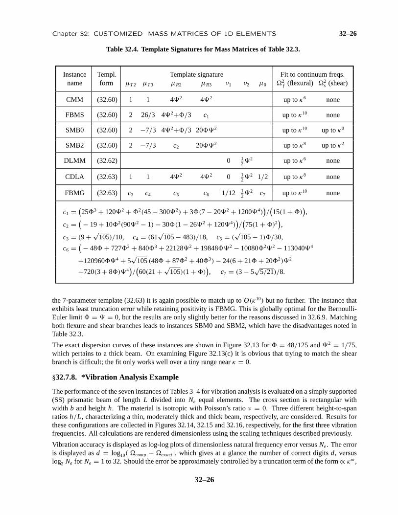
Table 32.4. Template Signatures for Mass Matrices of Table 32.3.

Instance Templ. Template signature Fit to continuum freqs.name form µT2 µT3 µR2 µR3 ν1 ν2 µ0 2

f (flexural) 2s (shear)

CMM (32.60) 1 1 42 42 up toκ6 none

FBMS (32.60) 2 26/3 42+/3 c1 up toκ10 none

SMB0 (32.60) 2 −7/3 42+/3 202 up toκ10 up toκ0

SMB2 (32.60) 2 −7/3 c2 202 up toκ8 up toκ2

DLMM (32.62) 0 122 up toκ6 none

CDLA (32.63) 1 1 42 42 0 122 1/2 up toκ8 none

FBMG (32.63) c3 c4 c5 c6 1/12 122 c7 up toκ10 none

c1 = (253 + 1202 + 2(45− 3002) + 3(7 − 202 + 12004)

)/(15(1 + )

),

c2 = ( − 19+ 102(902 − 1) − 30(1 − 262 + 1204))/(75(1 + )2

),

c3 = (9 + √105)/10, c4 = (61

√105− 483)/18, c5 = (

√105− 1)/30,

c6 = ( − 48 + 7272 + 8403 + 221282 + 198482 − 1008022 − 1130404

+1209604 + 5√

105(48 + 872 + 403) − 24(6 + 21 + 202)2

+720(3 + 8)4)/(60(21+ √

105)(1 + )), c7 = (3 − 5

√5/21)/8.

the 7-parameter template (32.63) it is again possible to match up toO(κ10) but no further. The instance thatexhibits least truncation error while retaining positivity is FBMG. This is globally optimal for the Bernoulli-Euler limit = = 0, but the results are only slightly better for the reasons discussed in 32.6.9. Matchingboth flexure and shear branches leads to instances SBM0 and SBM2, which have the disadvantages noted inTable 32.3.

The exact dispersion curves of these instances are shown in Figure 32.13 for = 48/125 and2 = 1/75,which pertains to a thick beam. On examining Figure 32.13(c) it is obvious that trying to match the shearbranch is difficult; the fit only works well over a tiny range nearκ = 0.

§32.7.8. *Vibration Analysis Example

The performance of the seven instances of Tables 3–4 for vibration analysis is evaluated on a simply supported(SS) prismatic beam of lengthL divided into Ne equal elements. The cross section is rectangular withwidth b and heighth. The material is isotropic with Poisson’s ratioν = 0. Three different height-to-spanratiosh/L, characterizing a thin, moderately thick and thick beam, respectively, are considered. Results forthese configurations are collected in Figures 32.14, 32.15 and 32.16, respectively, for the first three vibrationfrequencies. All calculations are rendered dimensionless using the scaling techniques described previously.

Vibration accuracy is displayed as log-log plots of dimensionless natural frequency error versusNe. The erroris displayed asd = log10(|comp − exact|, which gives at a glance the number of correct digitsd, versuslog2 Ne for Ne = 1 to 32. Should the error be approximately controlled by a truncation term of the form∝ κm,

32–26


0 1 2 3 4 5 6

10

20

30

40

50

60

0 1 2 3 4 5 6

10

20

30

40

50

60

0 1 2 3 4 5 6

10

20

30

40

50

60

0 1 2 3 4 5 6

10

20

30

40

50

60

Ω continuums

Ω CMMo

Ω DLMMo

Ω FBMSo

Ω CMMa

Ω continuumf

sΩ continuum

Ω CDLAo

Ω FBMGo

Ω SBM2o

Ω SBM0o

Ω continuumsΩ continuums

Ω continuumf

Ω continuumf

Ω continuumf

Ω FBMSa

Ω SBM2a

Ω FBMGaΩ CDLAa

Ω SBM0a

Dimensionless wavenumber κ= k




Dim

ensi

onle

ss fr

eque

ncy

Ω

Dim

ensi

onle

ss fr

eque

ncy

Ω

Dim

ensi

onle

ss fr

eque

ncy

Ω

Dim

ensi

onle

ss fr

eque

ncy

Ω

Ωcutoff

Ωcutoff

Ωcutoff

Ωcutoff

Ω DLMMa

Figure 32.13. Dimensionless dispersion curves of Timoshenko mass matrices instances of Tables 32.3–32.4 fora thick beam with0 = 48/125 = 0.384 and2

0 = 1/75 = 0.0133. (a) Curves for standard consistent anddiagonally-lumped matrices CMM and DLMM; (b) curves for the flexural-branch-matched FBMS and CDLA, (d)curves for the shear-branch-matched SBM0 and SBM2; (e) curve for flexure branch globally optimized FBMG.

the log-log plot should be roughly a straight line of slope∝ m, sinceκ = k = kL/Ne.

The results for the Bernoulli-Euler model, shown in Figure 32.14, agree perfectly with the truncation error inthe2

f branch as listed in Table 32.4. For example, top performers FBMG and FBMS gain digits twice as fastas CMM, DLMM and SBM2, since the formers match2

f to O(κ10) whereas the latter do that only toO(κ6).Instances CDLA and SMB0, which agree throughO(κ8), come in between. The highly complicated FBMGis only slightly better than the simpler FBMS. Their high accuracy case should be noted. For example, fourFBMS elements give1 to six figures: 9.86960281. . . versusπ2 = 9.86960440. . ., whereas CMM gives lessthan three: 9.87216716. . .. The “accuracy ceiling” of about 11 digits for FBMS and FBMG observable forNe > 16 is due to the eigensolver working in double precision (≈ 16 digits). Rerunning with higher (quad)floating point precision, the plots continues marching up as straight line before leveling at 25 digits.

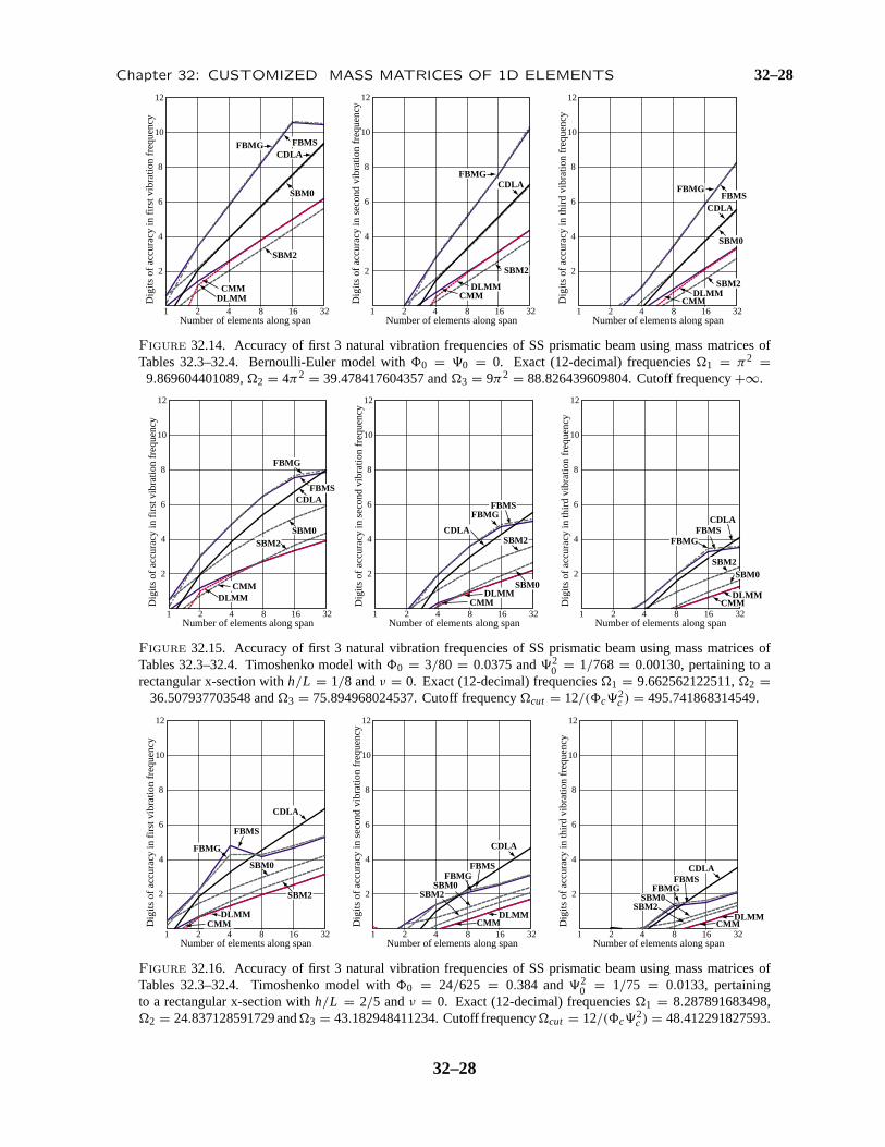
On passing to the Timoshenko model, the well ordered Bernoulli-Euler world of Figure 32.14 unravels. Theculprits are and. These figure prominently in the branch series and grow without bound asNe increases,as discussed in 32.6.2. Figure 32.15 collects results for a moderately thick beam withh/L = 1/8, whichcorresponds to0 = 3/80 and2

0 = 1/768. The Bernoulli-Euler top performers, FBMS and FBMG,gradually slow down and are caught by CDLA byNe = 32. All other instances trail, with the standard ones:CMM and DLMM, becoming the worst performers. Note that forNe = 32, CMM and DLMM provide only1 digit of accuracy in3 although there are 32/1.5 ≈ 21 elements per wavelength.

Figure 32.16 collects results for a thick beam withh/L = 2/5, corresponding to0 = 24/625 and20 = 1/75.

The foregoing trends are exacerbated, with FBMS and FBMG running out of steam byNe = 4 and CDLA

32–27


21 4 8 16 32

2

4

6

8

10

12

Number of elements along span

Dig

its o

f acc

urac

y in

firs

t vib

ratio

n fr

eque

ncy

21 4 8 16 32

2

4

6

8

10

12


Dig

its o

f acc

urac

y in

sec

ond

vibr

atio

n fr

eque

ncy

21 4 8 16 32

2

4

6

8

10

12


Dig

its o

f acc

urac

y in

third

vib

ratio

n fr

eque

ncy

FBMG

FBMG

FBMS

FBMSCDLA

SBM0

SBM0

SBM2

SBM2

CMMDLMM

DLMMDLMM

FBMG

CMMCMM

SBM2

CDLA

CDLA

Figure 32.14. Accuracy of first 3 natural vibration frequencies of SS prismatic beam using mass matrices ofTables 32.3–32.4. Bernoulli-Euler model with0 = 0 = 0. Exact (12-decimal) frequencies1 = π2 =9.869604401089,2 = 4π2 = 39.478417604357 and3 = 9π2 = 88.826439609804. Cutoff frequency+∞.

21 4 8 16 32

2

4

6

8

10

12


Dig

its o

f acc

urac

y in

third

vib

ratio

n fr

eque

ncy

21 4 8 16 32

2

4

6

8

10

12


Dig

its o

f acc

urac

y in

sec

ond

vibr

atio

n fr

eque

ncy

21 4 8 16 32

2

4

6

8

10

12


Dig

its o

f acc

urac

y in

firs

t vib

ratio

n fr

eque

ncy

FBMG

FBMG

FBMSCDLA

SBM0SBM2

DLMM DLMM DLMM

FBMG

FBMS

SBM0SBM0

CMM

CMM

CMM

SBM2

SBM2

CDLAFBMSCDLA

Figure 32.15. Accuracy of first 3 natural vibration frequencies of SS prismatic beam using mass matrices ofTables 32.3–32.4. Timoshenko model with0 = 3/80 = 0.0375 and2

0 = 1/768 = 0.00130, pertaining to arectangular x-section withh/L = 1/8 andν = 0. Exact (12-decimal) frequencies1 = 9.662562122511,2 =

36.507937703548 and3 = 75.894968024537. Cutoff frequencycut = 12/(c2c ) = 495.741868314549.

21 4 8 16 32

2

4

6

8

10

12


Dig

its o

f acc

urac

y in

third

vib

ratio

n fr

eque

ncy

21 4 8 16 32

2

4

6

8

10

12


Dig

its o

f acc

urac

y in

sec

ond

vibr

atio

n fr

eque

ncy

21 4 8 16 32

2

4

6

8

10

12


Dig

its o

f acc

urac

y in

firs

t vib

ratio

n fr

eque

ncy

FBMS

SBM0

SBM0SBM0SBM2 SBM2

SBM2DLMM DLMM DLMM

FBMG

FBMGFBMG

CMM CMM CMM

CDLA

CDLA

CDLAFBMS

FBMS

Figure 32.16. Accuracy of first 3 natural vibration frequencies of SS prismatic beam using mass matrices ofTables 32.3–32.4. Timoshenko model with0 = 24/625 = 0.384 and2

0 = 1/75 = 0.0133, pertainingto a rectangular x-section withh/L = 2/5 andν = 0. Exact (12-decimal) frequencies1 = 8.287891683498,2 = 24.837128591729 and3 = 43.182948411234. Cutoff frequencycut = 12/(c

2c ) = 48.412291827593.

32–28

32–29 §32. References

emerging as best forNe ≥ 8. Again DCLM and CMM trail badly.

The reason for the performance degradation of FBMS and FBMG as the Timoshenko beam gets thicker isunclear. Eigensolver accuracy is not responsible since rerunning the cases of Figures 32.15 and 32.16 in quadprecision did not change the plots. A numerical study of the2

f truncation error shows that FBMS and FBMGfit the continuum branch better than CDLA even for very thick beams. Possible contamination of vibrationmode shapes with the shear branch was not investigated.

Notes and Bibliography

The template approach addresses the deficiencies of the conventional mass models by using a parametrizationapproach that permits customization of that matrix to the problem and solution method at hand. The methodwas originally developed to construct high-performance stiffness matrices; a historical account and pertinentreferences are provided in a recent tutorial [61]. For stiffness-mass pairs it was used in [56,58] for a Bernoulli-Euler plane beam using Fourier analysis. One idea developed in those papers but not pursued here was toinclude the stiffness matrix template in the customization process. This provides more flexibility but has anegative side: highly optimized stiffness-mass pairs become sensitive to mesh distortion.

The symbolic derivation scheme used for the EOM (32.45) is due to Flaggs [63]; see also [126].

Making K andM frequency dependent was first proposed by Przemieniecki [140], who expanded bothKe

andMe as Taylor series inω2. The idea was applied to eigenfrequency analysis of bars and beams, but notpursued further. The approach can be generalized to the template context by making free parameters frequencydependent, as illustrate in the two-node bar example. This may be of interest for problems dominated by asingle driving frequency, as in some electronic and optical components. For more general use keeping theparameters frequency independent, as done in the last two examples, appears to be more practical.

Two powerful customization techniques used regularly for templates are Fourier methods and modified differ-ential equations (MoDE). Fourier methods are limited to separable systems but can be straightforward to apply,requiring only undergraduate mathematics. (As tutorials for applied Fourier methods Hamming’s textbooks[90,91], are recommended.) MoDE methods, first published in correct form in 1974 [181] are less restrictivebut more demanding on two fronts: mathematical ability and support of a computer algebra system (CAS).Processing power limitations presently restrict MoDE to two-dimensional elements and regular meshes. Theselection of template optimization criteria is not yet on firm ground. For example: is conservation of angularmomentum useful in mass templates? The answer seems to depend on the element complexity.

Results for regular lattices of structural elements have direct counterparts in a very different area: molecularphysics. More precisely, the wave mechanics of crystalline solids created in the XX Century by particlemechanicians; e.g., [22,197]. In crystal models, lattice nodes are occupied by molecules interacting withadjacent ones. Thus the “element dimension” acquires a physical meaning of molecular gap. In thoseapplications masses are alwayslumpedat molecule locations, and atoms vibrate as harmonic oscillators inthe potential well of the force fields of their neighbors. Dispersion curves govern energy transmission. In alinear atomic chain, the wavenumber rangeκ ∈ [−π, π ] is called the first Brillouin zone [23,104]. Such aconnection may be of interest as FEM and related discretization methods are extended into nano-mechanics.

References

Referenced items moved to Appendix R.

32–29


Homework Exercises for Chapter 32

Customized Mass Matrices of 1D Elements

EXERCISE 32.1 [A:10]. Express the Nyquist frequency for the 2-node bar lattice as function ofµ.

EXERCISE 32.2 [A:30]. Investigate the behavior of an infinite 2-node bar lattice where element lengthsalternate. Use either Fourier or MoDE.

EXERCISE 32.3 [A:25]. Investigate customized mass matrices for the 3-node bar without preimposing theangular moment conservation conditionµ1 = µ3. Use Fourier analysis on a lattice, stating from a 3-parametermass template.

32–30

Customized Mass Matrices of 1D Elements

Documents

Transcript of Customized Mass Matrices of 1D Elements