Curve3 Guide 006w - HutchColor · Curve3™ is a multi-purpose software calibration program...
124
Copyright © HutchColor, LLC. 1/124 Curve3_Guide_006v Second Edition Software Version 3.0.1 Document Version 006w October 2013 (www.hutchcolor.com/CurveGuide.htm) Copyright © HutchColor, LLC. • All rights reserved Curve2™ and Curve3™ are trademarks of HutchColor, LLC and CHROMiX, Inc • G7®, GRACoL® and SWOP® are registered trademarks of IDEAlliance, used with permission • All other product names and trademarks are the property of their respective owners
Transcript of Curve3 Guide 006w - HutchColor · Curve3™ is a multi-purpose software calibration program...
Copyright © HutchColor, LLC. 1/124 Curve3_Guide_006v
Second Edition
Software Version 3.0.1 Document Version 006w
October 2013 (www.hutchcolor.com/CurveGuide.htm)
Copyright © HutchColor, LLC. • All rights reserved
Curve2™ and Curve3™ are trademarks of HutchColor, LLC and CHROMiX, Inc • G7®, GRACoL® and SWOP® are registered trademarks of IDEAlliance, used with permission • All
other product names and trademarks are the property of their respective owners
USER GUIDE
Copyright © HutchColor, LLC. 2/124 Curve3_Guide_006v
C O N T E N T S
1. Introduction ...................................................................................................... 9 What is Curve3? ....................................................................................................................... 9 Differences Compared to Curve2 .......................................................................................... 10 Quick Look ............................................................................................................................. 10 4D Input Data Smoothing ..................................................................................................................... 10 Non-Linear Initial Calibration ................................................................................................................ 10 Custom Control-Point Lists .................................................................................................................. 11 Native Black Aim-Point ......................................................................................................................... 11 Normalize High Densities ...................................................................................................................... 11 Custom TVI Curves ............................................................................................................................... 11 Special Ink Calibration .......................................................................................................................... 11 Spectral VPR ........................................................................................................................................ 11 Enhanced Graphing and Reporting ...................................................................................................... 11 Expanded native RIP support ............................................................................................................... 11
Functionality Levels ............................................................................................................... 11 Demo Mode .......................................................................................................................................... 12 Verify Module ........................................................................................................................................ 12 Calibrate Module .................................................................................................................................. 12 Virtual Press Run Module ..................................................................................................................... 12
About this User Guide ............................................................................................................ 12 Typos, Errors or Suggestions ............................................................................................................... 14
System Requirements ............................................................................................................ 14 Differences Between Mac and Windows ............................................................................... 14 Installing and Registering Curve3 .......................................................................................... 14 Custom Folders for Control Points and Color Standards ...................................................... 14 Software Updates .................................................................................................................. 14 Reporting Software Problems ................................................................................................ 15 Maxwell users ....................................................................................................................................... 15
2. Software Principles ....................................................................................... 16 The Main Menu Bar ................................................................................................................ 16 Main Function Buttons ........................................................................................................... 16 Calibration Runs .................................................................................................................... 17 Output Product ...................................................................................................................... 17 Sessions ................................................................................................................................. 17 Creating a New Session ....................................................................................................................... 17 Saving a Session ................................................................................................................................... 17 Opening a Session ................................................................................................................................ 17
Working With Graphs ............................................................................................................. 17 Expanding and Contracting a graph ..................................................................................................... 18 Magnifying a Graph .............................................................................................................................. 18 Scrolling a Graph .................................................................................................................................. 18
Shortcut Keys ........................................................................................................................ 18 Up / Down arrows ................................................................................................................................. 18 Left / Right arrows ................................................................................................................................ 19 Shift + Left / Right arrows ..................................................................................................................... 19
3. Setup ............................................................................................................... 20 Curve Method ........................................................................................................................ 20 TVI Curve Selection ............................................................................................................... 21 Special Ink Calibration ........................................................................................................... 21
USER GUIDE
Copyright © HutchColor, LLC. 3/124 Curve3_Guide_006v
Measured vs. Wanted ............................................................................................................ 21 Information and Notes ........................................................................................................... 21
4. Ink Test ........................................................................................................... 23 Samples ................................................................................................................................. 23 Comparison Color Space ...................................................................................................... 24 Adding Custom Target Color Spaces .................................................................................... 24 Creating a Custom Color Space File .................................................................................................... 24
Results Panel ......................................................................................................................... 25 Densities ............................................................................................................................................... 25 Delta-E .................................................................................................................................................. 25
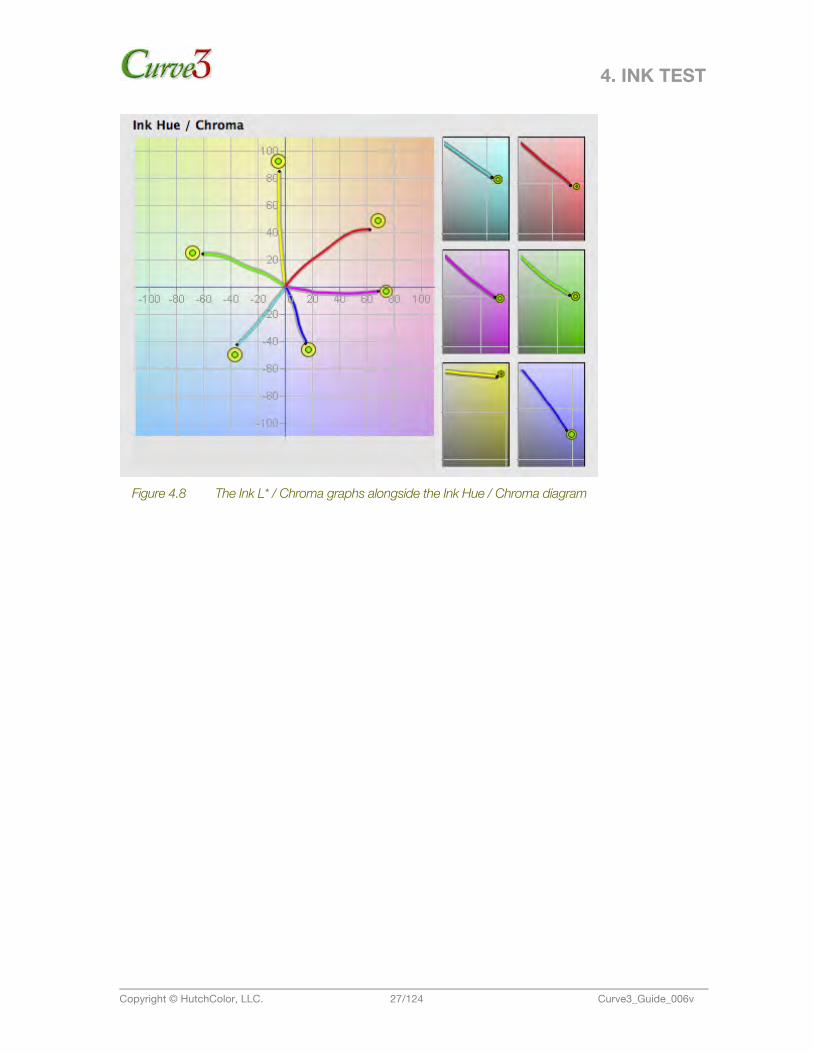
Ink Hue / Chroma Graph ........................................................................................................ 26 Ink L* / Chroma Graphs ......................................................................................................... 26
5. Calibrate ......................................................................................................... 28 The Calibrate Runs List .......................................................................................................... 28 Selecting a Calibration Run .................................................................................................................. 29 Creating New Calibration Runs ............................................................................................................ 29 Deleting a Calibration Run .................................................................................................................... 29 The Printing Guide ................................................................................................................................ 29 The Calibration Run Report .................................................................................................................. 29
The Measurements List ......................................................................................................... 29 Adding and Deleting Measurement Files .............................................................................................. 29 Disabling and Enabling Measurement Files .......................................................................................... 30 Measurement File Warning Colors ........................................................................................................ 30 Measurement File Delta-E Values ......................................................................................................... 30
The Smooth Button ................................................................................................................ 31 The Based On: List ................................................................................................................ 32 Basing on a Previous Session ............................................................................................................... 32 Basing on Arbitrary RIP Curves ............................................................................................................ 32
Function Tabs ........................................................................................................................ 32 The Measurements Panel ...................................................................................................... 33 NPDC Graphs ....................................................................................................................................... 33 Comparing NPDC of a Single Measurement File .................................................................................. 33 CMY Gray Balance ............................................................................................................................... 34 TVI (Dot Gain) Graph ............................................................................................................................. 34
The Analyze Panel .................................................................................................................. 34 Ink & Paper tab ..................................................................................................................................... 35 G7 tab ................................................................................................................................................... 35 Curve Shape graph .............................................................................................................................. 36 Gray Balance graph .............................................................................................................................. 36 TVI tab .................................................................................................................................................. 36 Run-to-Run tab ..................................................................................................................................... 37
The Create Curves Panel ....................................................................................................... 37 Choosing Control Point Values ............................................................................................................. 38 Adding/Subtracting Control Points ....................................................................................................... 38 Which Control Points? .......................................................................................................................... 38 Saving a Custom Control Point Set ...................................................................................................... 39 Delta Values vs Absolute values ........................................................................................................... 39 Wanted vs. Measured values ................................................................................................................ 39 Normalize High Densities ...................................................................................................................... 40 Export... ................................................................................................................................................ 42 Gray Balance ........................................................................................................................................ 42 Switching gray balance ON and OFF ................................................................................................... 42
The Gray Balance Control Tab .............................................................................................. 42 Gray Correction Feather-Off ................................................................................................................. 43
USER GUIDE
Copyright © HutchColor, LLC. 4/124 Curve3_Guide_006v
Precision Gray Balance and Blend Gray Samples ................................................................................ 43 The White / Black Tab ............................................................................................................ 44 White Aimpoint ..................................................................................................................................... 44 Using White Aimpoint with an ICC Profile ............................................................................................ 45 Black Aimpoint (300% CMY) ................................................................................................................ 45
The Printing Aims Tab ............................................................................................................ 46
6. Verify ............................................................................................................... 47 Curve3 Verify-Only Option ..................................................................................................... 47 G7 Verify Mode ...................................................................................................................... 47 Samples list .......................................................................................................................................... 48 Ink & Paper Test .................................................................................................................................... 48 G7 tab ................................................................................................................................................... 48 Results chart ......................................................................................................................................... 49 Curve Shape (delta-L*) graph ............................................................................................................... 49 Gray Balance graph .............................................................................................................................. 49 Weighting Function ............................................................................................................................... 50 G7 Tolerances ....................................................................................................................................... 50
TVI Verify Mode ...................................................................................................................... 50
7. VPR (Virtual Press Run) ................................................................................. 51 Activating the VPR Module .................................................................................................... 51 Benefits of VPR ...................................................................................................................... 51 Difference between Curve2 and Curve3 VPR ........................................................................ 52 How VPR Works .................................................................................................................... 52 Understanding the VPR concept .......................................................................................................... 52
Target data to be curved: ...................................................................................................... 53 Training Target ....................................................................................................................... 53 Curving Method ..................................................................................................................... 53 Curve Lab values .................................................................................................................................. 53 Curve Spectral values ........................................................................................................................... 53 Curve CMYK values .............................................................................................................................. 54
Applying VPR to a Characterization Target ........................................................................... 54 Applying VPR to Non-Characterization Data ......................................................................... 54 Calibrating Without a P2P Target .......................................................................................... 54 Creating a Null Calibration Run ............................................................................................................ 54 Extracting P2P data from a characterization data set ........................................................................... 55 Using the extracted P2P data ............................................................................................................... 55
OneRun Targets ..................................................................................................................... 55 Available OneRun Targets .................................................................................................................... 55 Using OneRun Targets ......................................................................................................................... 56
Optimizing or Smoothing Characterization Data ................................................................... 56 Optimizing the Data .............................................................................................................................. 57
8. G7 Calibration Workflow ............................................................................... 58 Workflow Summary ................................................................................................................ 58 Print the P2P target(s) ............................................................................................................ 58 Measure the P2P targets ....................................................................................................... 58 Load measurement files into Curve3 ..................................................................................... 58 Select Based On: Status ........................................................................................................ 59 Adjust gray balance parameters ............................................................................................ 59 Choose Control Points ........................................................................................................... 59 Apply Control Points values to the RIP .................................................................................. 59 Print a new P2P Target through new curves ......................................................................... 59 Verify G7 calibration accuracy ............................................................................................... 59
USER GUIDE
Copyright © HutchColor, LLC. 5/124 Curve3_Guide_006v
Verifying G7 calibration with a new Run ............................................................................................... 59 Using the G7 Verify window ................................................................................................................. 60
9. TVI Calibration Workflow .............................................................................. 61 Workflow Summary ................................................................................................................ 61 Print the P2P target(s) ............................................................................................................ 61 Measure the P2P targets ....................................................................................................... 61 Change Calibration mode to TVI ............................................................................................ 61 Select TVI Target Curves ....................................................................................................... 62 Working with custom TVI Target Curves ............................................................................... 62 Load measurement files into Curve3 ..................................................................................... 62 Choose Control Points ........................................................................................................... 62 Leave Gray Balance ON ........................................................................................................ 62 Apply Control Points values to the RIP .................................................................................. 62 Print a new Target through new curves ................................................................................. 62 Verify TVI calibration accuracy ............................................................................................... 63 Verifying TVI calibration with a new Run ............................................................................................... 63
10. Special Ink Calibration Workflow ................................................................. 64 Workflow Summary ................................................................................................................ 64 Print the P2P target(s) ............................................................................................................ 64 Measure the P2P targets ....................................................................................................... 64 Change Calibration mode to Special Inks ............................................................................. 64 Load measurement files into Curve3 ..................................................................................... 65 Choose Control Points ........................................................................................................... 65 Ignore the Gray Balance Switch ............................................................................................ 65 Apply Control Point values to the RIP ................................................................................... 65 Print a new Target through new curves ................................................................................. 65 Verify Special Ink calibration accuracy .................................................................................. 65 Verifying Special Ink calibration with a new Run .................................................................................. 65
11. Applying Calibration Values .......................................................................... 66 Transferring Curve Values to a RIP ........................................................................................ 66 Manual entry ......................................................................................................................................... 66 Digital entry ........................................................................................................................................... 67
Basic Calibration Principles ................................................................................................... 67 CMYK+ Calibration ............................................................................................................................... 67 Calibration naming conventions ........................................................................................................... 68 Control points (a.k.a. file values or initial values) ................................................................................... 68 Measured values ................................................................................................................................... 68 Wanted values ...................................................................................................................................... 68
Measured vs. Wanted Values ................................................................................................ 69 If the RIP does not accept Wanted values ............................................................................................ 69
G7 Calibration vs. Plate Linearization .................................................................................... 69 Pre-Linearized Method .......................................................................................................... 69 Initial Linearization ................................................................................................................................ 69 G7 Calibration ....................................................................................................................................... 70 Re-Linearization .................................................................................................................................... 70
Post-Linearized Method ........................................................................................................ 70 Initial Plate Setup .................................................................................................................................. 70 G7 Calibration ....................................................................................................................................... 70 Post-Linearization on Top of G7 Calibration ......................................................................................... 71 Post-Linearization Without G7 Calibration ............................................................................................ 71
Calibrating Via a DLP ............................................................................................................. 72 Saving a DLP from Curve3 ................................................................................................................... 72
USER GUIDE
Copyright © HutchColor, LLC. 6/124 Curve3_Guide_006v
Choosing Measured vs Wanted with DLPs .......................................................................................... 72 Using a DLP in a Photoshop workflow ................................................................................................. 72 Testing RIP accuracy via Photoshop .................................................................................................... 73
Calibrating Via Photoshop Curves ......................................................................................... 74 Saving a Photoshop curve from Curve3 ............................................................................................... 74 Using a Curve3-generated Photoshop curve ....................................................................................... 75
Unit values and precision ....................................................................................................... 75
12. RIP-Specific Notes ........................................................................................ 76 Export File Type List .............................................................................................................. 76 Agfa :Apogee ......................................................................................................................... 76 Caldera ................................................................................................................................... 77 CREO Prinergy (Harmony Curves) ......................................................................................... 78 Constructing a Custom Linear Current curve in Harmony .................................................................... 78 Constructing a Custom Linear Target curve in Harmony ...................................................................... 78 Constructing a Custom Linear Calibration curve in Harmony ............................................................... 78
EFI .......................................................................................................................................... 79 G7 Curve only (G7 unmanaged): .......................................................................................................... 79 G7 Curve applied to GRACoL Source and existing Output profile (G7 simulated): .............................. 81 Output profile created with G7 Curve (G7 simulated): .......................................................................... 83
ErgoSoft ................................................................................................................................. 84 Items needed ........................................................................................................................................ 84 Process description .............................................................................................................................. 84 Create calibration curves in Curve3 ...................................................................................................... 85 Import the calibration into ErgoSoft ..................................................................................................... 86 Validation .............................................................................................................................................. 86
ESKO Nexus / Symphony ...................................................................................................... 86 ESKO IntelliCurve .................................................................................................................. 88 HP Indigo ............................................................................................................................... 88 Print the P2P26 target .......................................................................................................................... 88 Export HP Indigo File set ...................................................................................................................... 88 Import LUTs into HP Production Manager ........................................................................................... 89
Kodak Approval (XP4) ............................................................................................................ 90 Konica Minolta IC601 ............................................................................................................. 90 ONYX ..................................................................................................................................... 90 Overview ............................................................................................................................................... 90 Creating a G7 Media Model .................................................................................................................. 90 Verifying the G7 Media Model .............................................................................................................. 93
Working With Incompatible RIPs ........................................................................................... 95
13. Iteration .......................................................................................................... 96 The Basis Run ........................................................................................................................ 96 How Iteration Works .............................................................................................................. 97 Applying Iterated Calibration Values ...................................................................................... 98 The Importance of Saving Sessions ..................................................................................................... 98 If You Don’t Have a Saved Session ...................................................................................................... 98
Creating and using an Initial Curves File ............................................................................... 98 Working with an Initial Curves file ......................................................................................................... 98
Precision Limits ...................................................................................................................... 99 Avoiding Errors .................................................................................................................... 100
14. Tips and Trouble-Shooting ......................................................................... 101 Incorrect i1iO Alignment ...................................................................................................... 101 Corrective Action ................................................................................................................................ 101
Uneven Printing ................................................................................................................... 101 Corrective Action ................................................................................................................................ 102
USER GUIDE
Copyright © HutchColor, LLC. 7/124 Curve3_Guide_006v
Density Reversals ................................................................................................................ 104 Corrective Action ................................................................................................................................ 104
G7 Extreme Saturated Detail ............................................................................................... 105 Corrective Action ................................................................................................................................ 105
P2P Target Variations .......................................................................................................... 106 P2P27 ................................................................................................................................................. 107 P2P26 ................................................................................................................................................. 107 P2P? ................................................................................................................................................... 107
Mixed P2P Files ................................................................................................................... 107
A. Target Printing ............................................................................................. 108 Establishing a Base-line Condition ...................................................................................... 108 Ink-limiting .......................................................................................................................................... 108 G7 calibration and ICC color management ........................................................................................ 108
The P2P25 Target ................................................................................................................ 108 Older P2P Targets ............................................................................................................... 109 Working With Non-Standard P2P Targets ........................................................................... 109 Custom-Generated and Odd-Size Targets .......................................................................... 110 Printing the P2P Target ........................................................................................................ 110 Back-side printing ............................................................................................................................... 110
Printing Multiple P2P targets ............................................................................................... 110 Averaging Multiple Print Runs .............................................................................................. 110
B. Target Measuring ........................................................................................ 111 Measuring the P2P .............................................................................................................. 111 Drying Time .......................................................................................................................... 111 Coatings ............................................................................................................................... 111
C. The Printing Guide ....................................................................................... 112 Grays Panel .......................................................................................................................... 113 Target ND ........................................................................................................................................... 113 Target Lab ........................................................................................................................................... 113 Gray Densities ..................................................................................................................................... 113
Solids Panel ......................................................................................................................... 114 L* a* b* ................................................................................................................................................ 114 Solid Densities .................................................................................................................................... 114
D. Calibration Run Report ............................................................................... 115 Control Points List ............................................................................................................... 116 NPDC Graphs, ∆E, ∆L*, ∆Ch* .............................................................................................. 116 Delta-L* and Gray Balance Graphs ...................................................................................... 117 The Delta-L* graph .............................................................................................................................. 117 The ∆Ch (green) line on the Gray Balance graph ................................................................................ 117 The a* and b* (pink and blue) lines on the Gray Balance graph .......................................................... 117
Solid Colors Chart ................................................................................................................ 117 Correction Curves ................................................................................................................ 118 TVI Curves ............................................................................................................................ 118 TVI calculations ................................................................................................................................... 118
E. References ................................................................................................... 119 Delta-Ch ............................................................................................................................... 119 Naming ............................................................................................................................................... 119 Usefulness .......................................................................................................................................... 119
Curve3 File Formats and Data Types .................................................................................. 120 File Formats Accepted by Curve3 ...................................................................................................... 120 Colorimetric Data Types Accepted by Curve3 ................................................................................... 120
USER GUIDE
Copyright © HutchColor, LLC. 8/124 Curve3_Guide_006v
F. Custom TVI Curves ..................................................................................... 121 Creating a Custom TVI Target Curve ................................................................................... 121 TVI Calculations ................................................................................................................... 122 Calculating XYZ-based TVI Target Values ........................................................................... 122
G. G7 Via Color Management .......................................................................... 123 No RIP Curves? ................................................................................................................... 123 Limitations ............................................................................................................................ 123 G7-Based Reference Print Conditions ................................................................................ 124 TR015 ................................................................................................................................................. 124 CGATS.21 ........................................................................................................................................... 124

USER GUIDE
Copyright © HutchColor, LLC. 9/124 Curve3_Guide_006v
1. 1. Introduction This section explains…
• What is Curve3 • Differences compared to Curve2 • Functionality levels • How to use this guide • Installation and registration • Updates and problem reporting
Figure 1.1 The Curve3 Splash Screen
What is Curve3? Curve3™ is a multi-purpose software calibration program designed to simplify the IDEAlliance G7® calibration method. Curve3 is the direct descendent of two previous software generations: Curve2™ (2009) and IDEAlink Curve™ (2006), which was the world’s first G7 calibration tool.
1. INTRODUCTION
Copyright © HutchColor, LLC. 10/124 Curve3_Guide_006v
With Curve3 you can: • Calibrate any stable printing system to match the G7 specification • Calibrate by the legacy TVI method to match ISO-standard TVI curves or user-created
custom TVI curve sets • Calibrate “special” inks that are not part of a normal CMYK four color set • Verify whether an ink and substrate combination meets the tolerances of a printing
specification such as GRACoL® or SWOP®, prior to calculating calibration curves • Verify calibration accuracy of a sample print against the G7 specification
With the optional VPR (Virtual Press Run) module you can: • Convert a characterization file measured from an un-calibrated device into values that
would be measured after calibration • Optimize a characterization data set to reduce the effects of uneven printing or
measurement errors
Differences Compared to Curve2 While maintaining the same proven performance of Curve2, Curve3 adds some exciting new quality, functionality and convenience enhancements like:
• 4D input data smoothing for unstable systems or data • User-specified non-linear initial calibration • Save and load user-defined Control Point lists • Measured-black aim-point to improve digital press calibration • Normalize High Densities option to suppress unnatural shadow contrast • User-defined custom TVI target curves • Special ink calibration for CMYK+ printing • Spectral VPR applies curves to full spectral data • Enhanced graphing and reporting • Expanded native RIP support
Quick Look If you’re already familiar with Curve2, here’s a quick look at what each new feature means. You’ll find more details in the main body of this guide.
4D Input Data Smoothing In Create Curves the Smooth button removes some of the worst data errors due to printing unevenness or measurement problems. Switching on Smooth typically gives a better calibration when only a limited number of measured samples are available and/or the printing or measuring systems are unstable or unreliable.
Non-Linear Initial Calibration In Create Curves a set of pre-existing plate curves can be loaded via the Based On: list. This is valuable when your first press run or print was made through non-linear RIP curves. Section 5 explains how to create and load a pre-existing plate curve file.
1. INTRODUCTION
Copyright © HutchColor, LLC. 11/124 Curve3_Guide_006v
Custom Control-Point Lists In Create Curves you can now save and load custom Control Point lists. If you save these in a folder called “Control Point Files” located in the folder from which Curve3 launches, your custom lists will appear in the pop-up menu of Control Point sets.
Native Black Aim-Point In the Create Curves – White/Black tab, the As Printed button changes the gray balance algorithm above 50% to aim for the printing system’s “native” printed color at 300% CMY, instead G7’s perfect neutral. On systems with a strongly colored 300% CMY patch, As Printed leads to smoother calibration curves and better ICC profiles, with little change in overall appearance.
CAUTION: As Printed may cause the system to fail G7 and should only be used when the 300% patch cannot be made neutral by physical press or ink adjustments.
Normalize High Densities In the Create Curves window, the Normalize High Densities button is designed to minimize curve artifacts such as sharp bends in the high density end of the CMY calibration curves. This can result in much smoother tonality in high density areas of the image, and lead to better ICC profiles.
CAUTION: Normalize High Densities may cause the system to fail G7 and should only be used when the CMY curves show sharp tone changes above 50% (see Troubleshooting for examples).
Custom TVI Curves In Setup - TVI custom TVI curves can now be loaded as well as the six standard TVI curves from ISO 12647-2. Section 9 and Appendix: F explain how to work with custom TVI curves.
Special Ink Calibration Special Ink calibration lets you calibrate non-CMYK inks using a simple, universal algorithm based on Delta E. Being Lab-based, it doesn’t require spectral data, the same algorithm is used for all inks, and the resulting calibration curves are typically nearly linear – similar to legacy calibrations.
This non-proprietary algorithm has been proposed to IDEAlliance as a possible standard. If another method is chosen, the new algorithm will be included in future Curve3 versions.
Spectral VPR VPR can now be applied to spectral measurements as well as Lab or XYZ files.
Enhanced Graphing and Reporting The Ink Hue / Chroma graph is now augmented with six L* / Chroma graphs showing the L* vector of each ink scale, while the Results chart adds solid ink Lab values as well as Delta E.
Expanded native RIP support Curve3 can export calibration data in the native RIP formats of a number of new RIPs and controllers. New RIPs will be added when available, so be sure you are using the latest version.
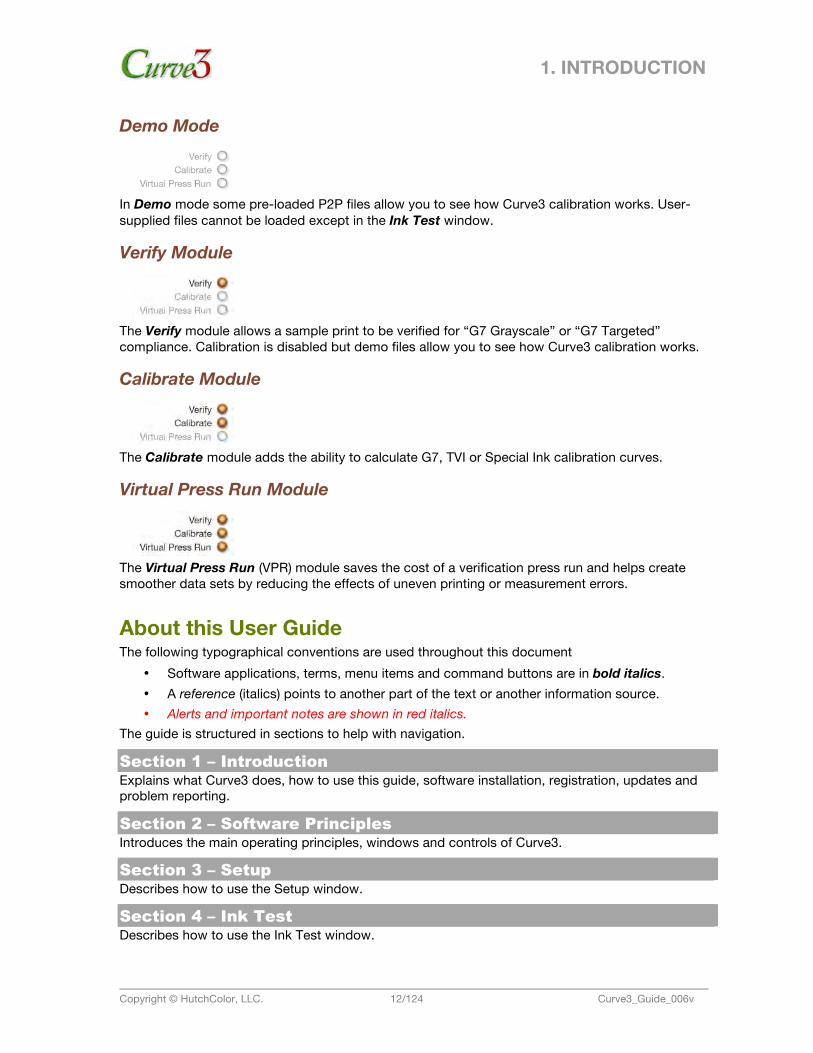
Functionality Levels Curve3 consists of three modules, or functionality levels, which are activated at three price levels. Each paid module includes all the functionality of the previous module(s). When no modules are active, the software enters Demo mode. The number of licensed modules is shown on the splash screen, as follows:
1. INTRODUCTION
Copyright © HutchColor, LLC. 12/124 Curve3_Guide_006v
Demo Mode
In Demo mode some pre-loaded P2P files allow you to see how Curve3 calibration works. User-supplied files cannot be loaded except in the Ink Test window.
Verify Module
The Verify module allows a sample print to be verified for “G7 Grayscale” or “G7 Targeted” compliance. Calibration is disabled but demo files allow you to see how Curve3 calibration works.
Calibrate Module
The Calibrate module adds the ability to calculate G7, TVI or Special Ink calibration curves.
Virtual Press Run Module
The Virtual Press Run (VPR) module saves the cost of a verification press run and helps create smoother data sets by reducing the effects of uneven printing or measurement errors.
About this User Guide The following typographical conventions are used throughout this document
• Software applications, terms, menu items and command buttons are in bold italics. • A reference (italics) points to another part of the text or another information source. • Alerts and important notes are shown in red italics.
The guide is structured in sections to help with navigation.
Section 1 – Introduction Explains what Curve3 does, how to use this guide, software installation, registration, updates and problem reporting.
Section 2 – Software Principles Introduces the main operating principles, windows and controls of Curve3.
Section 3 – Setup Describes how to use the Setup window.
Section 4 – Ink Test Describes how to use the Ink Test window.
1. INTRODUCTION
Copyright © HutchColor, LLC. 13/124 Curve3_Guide_006v
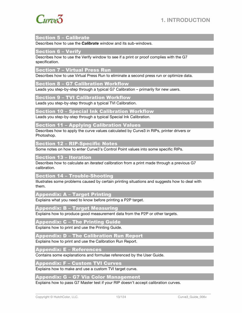
Section 5 – Calibrate Describes how to use the Calibrate window and its sub-windows.
Section 6 – Verify Describes how to use the Verify window to see if a print or proof complies with the G7 specification.
Section 7 – Virtual Press Run Describes how to use Virtual Press Run to eliminate a second press run or optimize data.
Section 8 – G7 Calibration Workflow Leads you step-by-step through a typical G7 Calibration – primarily for new users.
Section 9 – TVI Calibration Workflow Leads you step-by-step through a typical TVI Calibration.
Section 10 – Special Ink Calibration Workflow Leads you step-by-step through a typical Special Ink Calibration.
Section 11 – Applying Calibration Values Describes how to apply the curve values calculated by Curve3 in RIPs, printer drivers or Photoshop.
Section 12 – RIP-Specific Notes Some notes on how to enter Curve3’s Control Point values into some specific RIPs.
Section 13 – Iteration Describes how to calculate an iterated calibration from a print made through a previous G7 calibration.
Section 14 – Trouble-Shooting Illustrates some problems caused by certain printing situations and suggests how to deal with them.
Appendix: A – Target Printing Explains what you need to know before printing a P2P target.
Appendix: B – Target Measuring Explains how to produce good measurement data from the P2P or other targets.
Appendix: C – The Printing Guide Explains how to print and use the Printing Guide.
Appendix: D – The Calibration Run Report Explains how to print and use the Calibration Run Report.
Appendix: E – References Contains some explanations and formulae referenced by the User Guide.
Appendix: F – Custom TVI Curves Explains how to make and use a custom TVI target curve.
Appendix: G – G7 Via Color Management Explains how to pass G7 Master test if your RIP doesn’t accept calibration curves.
1. INTRODUCTION
Copyright © HutchColor, LLC. 14/124 Curve3_Guide_006v
Typos, Errors or Suggestions To report errors or suggestions concerning this User Guide, please contact [email protected].
System Requirements Curve3 is a stand-alone software available for Mac OS X and Windows XP or later.
IMPORTANT: Once installed, there is a charge to change your Curve3 license to another OS.
Differences Between Mac and Windows Apart from some cosmetic differences, the Mac and Windows versions of Curve3 are functionality identical.
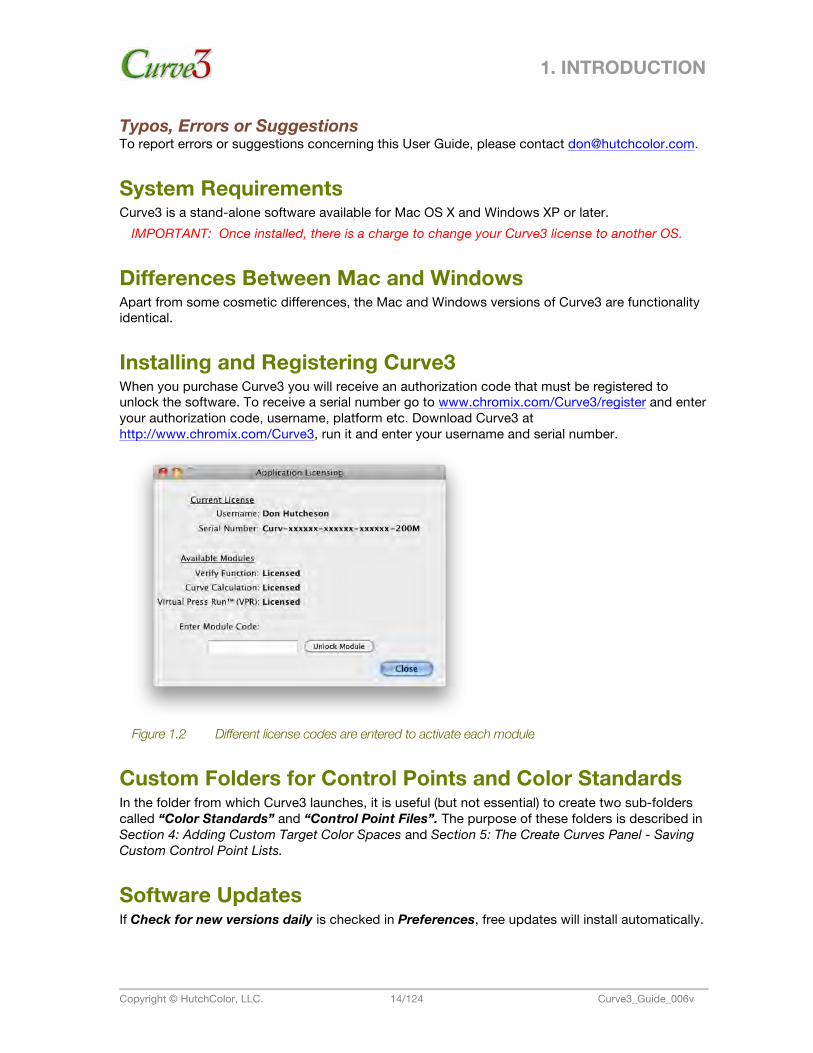
Installing and Registering Curve3 When you purchase Curve3 you will receive an authorization code that must be registered to unlock the software. To receive a serial number go to www.chromix.com/Curve3/register and enter your authorization code, username, platform etc. Download Curve3 at http://www.chromix.com/Curve3, run it and enter your username and serial number.
Figure 1.2 Different license codes are entered to activate each module
Custom Folders for Control Points and Color Standards In the folder from which Curve3 launches, it is useful (but not essential) to create two sub-folders called “Color Standards” and “Control Point Files”. The purpose of these folders is described in Section 4: Adding Custom Target Color Spaces and Section 5: The Create Curves Panel - Saving Custom Control Point Lists.
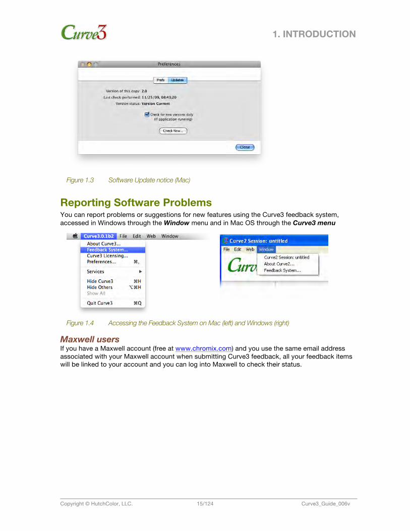
Software Updates If Check for new versions daily is checked in Preferences, free updates will install automatically.
1. INTRODUCTION
Copyright © HutchColor, LLC. 15/124 Curve3_Guide_006v
Figure 1.3 Software Update notice (Mac)
Reporting Software Problems You can report problems or suggestions for new features using the Curve3 feedback system, accessed in Windows through the Window menu and in Mac OS through the Curve3 menu
Figure 1.4 Accessing the Feedback System on Mac (left) and Windows (right)
Maxwell users If you have a Maxwell account (free at www.chromix.com) and you use the same email address associated with your Maxwell account when submitting Curve3 feedback, all your feedback items will be linked to your account and you can log into Maxwell to check their status.
USER GUIDE
Copyright © HutchColor, LLC. 16/124 Curve3_Guide_006v
2. 2. Software Principles This section introduces the main operating principles, windows and controls in Curve3.
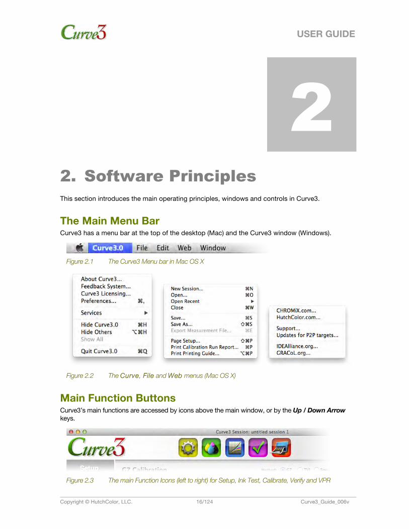
The Main Menu Bar Curve3 has a menu bar at the top of the desktop (Mac) and the Curve3 window (Windows).
Figure 2.1 The Curve3 Menu bar in Mac OS X
Figure 2.2 The Curve, File and Web menus (Mac OS X)
Main Function Buttons Curve3’s main functions are accessed by icons above the main window, or by the Up / Down Arrow keys.
Figure 2.3 The main Function Icons (left to right) for Setup, Ink Test, Calibrate, Verify and VPR
2. SOFTWARE PRINCIPLES
Copyright © HutchColor, LLC. 17/124 Curve3_Guide_006v
Each function is described in detail within its own section of this document.
Calibration Runs The main unit of work in Curve3 is the Calibration Run. A Calibration Run refers to a single print run or test print. Data files from the Calibration Run are loaded into Curve3 as measurement files created by measuring the P2P target in software like basICColor Catch™, Konica Minolta Color Care™, X-Rite i1Profiler™, X-Rite MeasureTool or X-Rite ColorPort. For more details on printing and measuring, see Appendix: A and Appendix: B.
Output Product The product of a Calibration Run is a list of CMYK Curve Point values or Calibration Curves that, when entered into the printer or RIP, should result in a properly calibrated print.
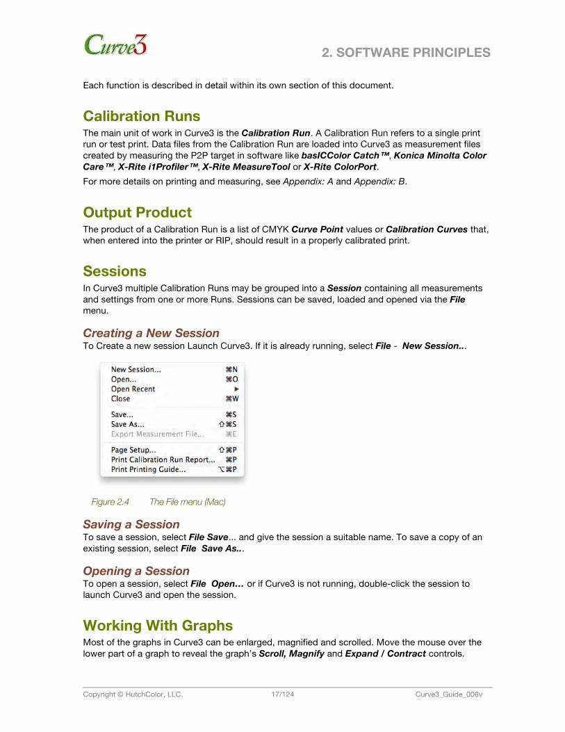
Sessions In Curve3 multiple Calibration Runs may be grouped into a Session containing all measurements and settings from one or more Runs. Sessions can be saved, loaded and opened via the File menu.
Creating a New Session To Create a new session Launch Curve3. If it is already running, select File - New Session...
Figure 2.4 The File menu (Mac)
Saving a Session To save a session, select File Save... and give the session a suitable name. To save a copy of an existing session, select File Save As...
Opening a Session To open a session, select File Open… or if Curve3 is not running, double-click the session to launch Curve3 and open the session.
Working With Graphs Most of the graphs in Curve3 can be enlarged, magnified and scrolled. Move the mouse over the lower part of a graph to reveal the graph’s Scroll, Magnify and Expand / Contract controls.
2. SOFTWARE PRINCIPLES
Copyright © HutchColor, LLC. 18/124 Curve3_Guide_006v
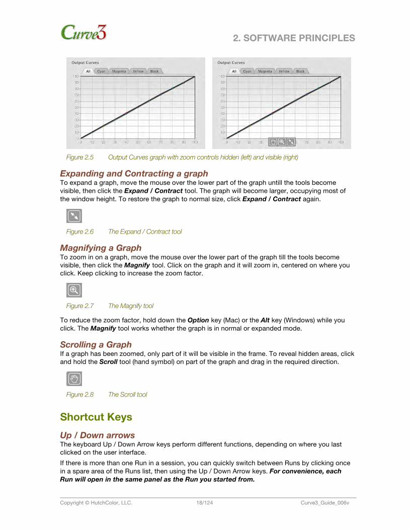
Figure 2.5 Output Curves graph with zoom controls hidden (left) and visible (right)
Expanding and Contracting a graph To expand a graph, move the mouse over the lower part of the graph untill the tools become visible, then click the Expand / Contract tool. The graph will become larger, occupying most of the window height. To restore the graph to normal size, click Expand / Contract again.
Figure 2.6 The Expand / Contract tool
Magnifying a Graph To zoom in on a graph, move the mouse over the lower part of the graph till the tools become visible, then click the Magnify tool. Click on the graph and it will zoom in, centered on where you click. Keep clicking to increase the zoom factor.
Figure 2.7 The Magnify tool
To reduce the zoom factor, hold down the Option key (Mac) or the Alt key (Windows) while you click. The Magnify tool works whether the graph is in normal or expanded mode.
Scrolling a Graph If a graph has been zoomed, only part of it will be visible in the frame. To reveal hidden areas, click and hold the Scroll tool (hand symbol) on part of the graph and drag in the required direction.
Figure 2.8 The Scroll tool
Shortcut Keys Up / Down arrows The keyboard Up / Down Arrow keys perform different functions, depending on where you last clicked on the user interface. If there is more than one Run in a session, you can quickly switch between Runs by clicking once in a spare area of the Runs list, then using the Up / Down Arrow keys. For convenience, each Run will open in the same panel as the Run you started from.

2. SOFTWARE PRINCIPLES
Copyright © HutchColor, LLC. 19/124 Curve3_Guide_006v
If there is more than one File in the Measurements list, you can quickly switch between Runs by clicking once in a spare area of the Measurements list, then using the Up / Down Arrow keys. If you are not in either the Runs or Measurements list, the Up / Down arrow keys will also move between the main Function windows, similar to clicking the main icons.
Left / Right arrows In a window with tabbed panels, such as Calibrate, use the Left / Right Arrow keys to move between that window’s tabs.
Figure 2.9 The left/ right Arrow reminder prompt
Shift + Left / Right arrows In a panel with tabs, such as Analyze or Create Curves, use the Shift-left Arrow and Shift-right Arrow keys to move between that panel’s tabs.
Figure 2.10 The shift-left/ right Arrow reminder prompt
USER GUIDE
Copyright © HutchColor, LLC. 20/124 Curve3_Guide_006v
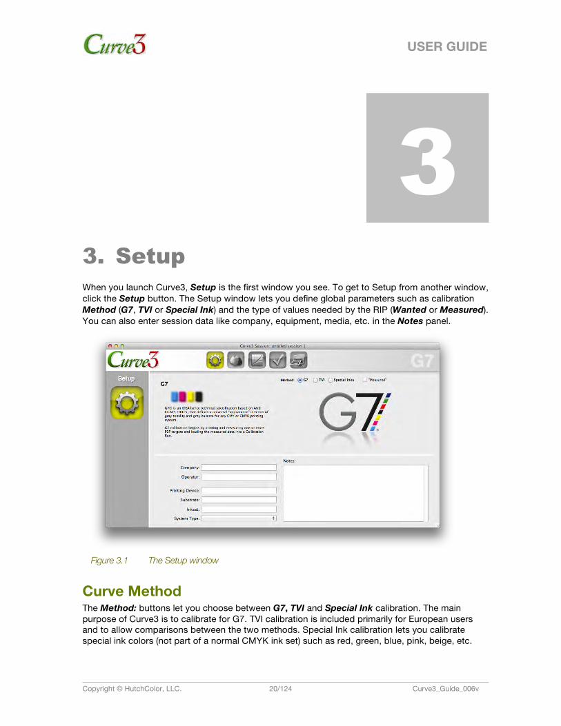
3. 3. Setup When you launch Curve3, Setup is the first window you see. To get to Setup from another window, click the Setup button. The Setup window lets you define global parameters such as calibration Method (G7, TVI or Special Ink) and the type of values needed by the RIP (Wanted or Measured). You can also enter session data like company, equipment, media, etc. in the Notes panel.
Figure 3.1 The Setup window
Curve Method The Method: buttons let you choose between G7, TVI and Special Ink calibration. The main purpose of Curve3 is to calibrate for G7. TVI calibration is included primarily for European users and to allow comparisons between the two methods. Special Ink calibration lets you calibrate special ink colors (not part of a normal CMYK ink set) such as red, green, blue, pink, beige, etc.
3. SETUP
Copyright © HutchColor, LLC. 21/124 Curve3_Guide_006v
Figure 3.2 Calibration method options
TVI Curve Selection When calibrating by the TVI method, you can choose one of the standard ISO 12647-2 TVI curves or your own custom TVI reference curves, as described in Section 9.
Note: TVI calibration has nothing to do with the G7 specification
Special Ink Calibration Up to four non-CMYK inks can be calibrated at once by printing the P2P target with any inks you like, replacing the normal C, M, Y and K inks. For more information see Section 10.
Note: Special Ink calibration has nothing to do with the G7 specification
Measured vs. Wanted If your RIP only accepts ‘Measured’ values (there is no place to enter Wanted values), click the Measured box in the Setup window. Otherwise leave it set to Wanted.
Figure 3.3 The ‘Measured’ option
Clicking Measured changes the Control Point percentage values and curve graphs in the Create Curves window. For more information see Section 5.
Figure 3.4 Effect of ‘Measured’ control on the Control Points in the Create Curves window
Information and Notes In the left half of the Setup window, optional data entry fields accept information about the device, media, etc. which will be included on the Printing Guide and Calibration Run Report.
3. SETUP
Copyright © HutchColor, LLC. 22/124 Curve3_Guide_006v
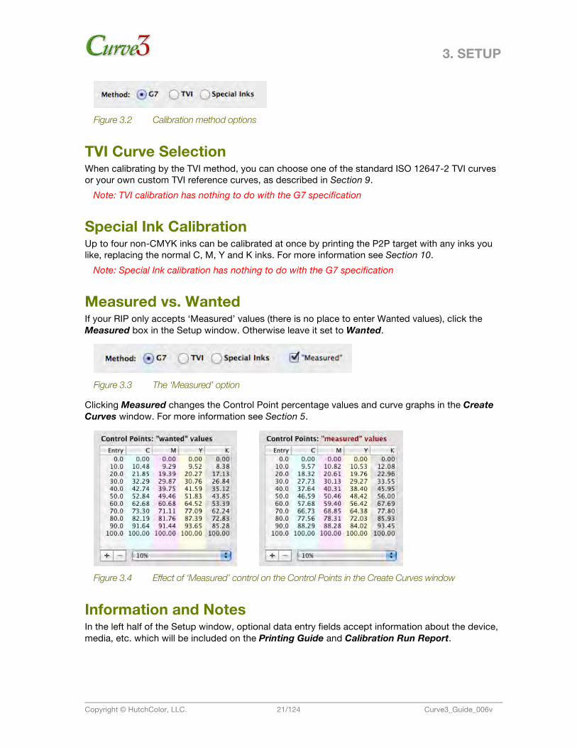
Figure 3.5 The setup window showing fields for basic information to be saved with the session
The Notes box provides room for other information about the session such as unusual operating conditions, problems encountered during the run, any particular reasons for the exercise, or what you had for lunch.
USER GUIDE
Copyright © HutchColor, LLC. 23/124 Curve3_Guide_006v
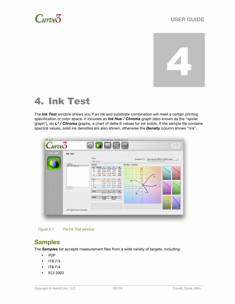
4. 4. Ink Test The Ink Test window shows you if an ink and substrate combination will meet a certain printing specification or color space. It includes an Ink Hue / Chroma graph (also known as the “spider graph”), six L* / Chroma graphs, a chart of delta-E values for ink solids. If the sample file contains spectral values, solid ink densities are also shown, otherwise the Density column shows “n/a”.
Figure 4.1 The Ink Test window
Samples The Samples list accepts measurement files from a wide variety of targets, including:
• P2P • IT8.7/3 • IT8.7/4 • ECI 2002
4. INK TEST
Copyright © HutchColor, LLC. 24/124 Curve3_Guide_006v
• HC2052 • IDEAlliance ISO 12647-7 Control Strip • Ugra/Fogra Media Wedge CMYK
Measurement files from custom targets can also be used so long as they are in CGATS format. There is no practical limit to how many patches you can have in a sample file. Curve3 automatically finds the solid ink and substrate values based on each entry’s CMYK values. Although multiple measurement files can be added to the Samples list, results are only shown for the single sample file highlighted in the list.
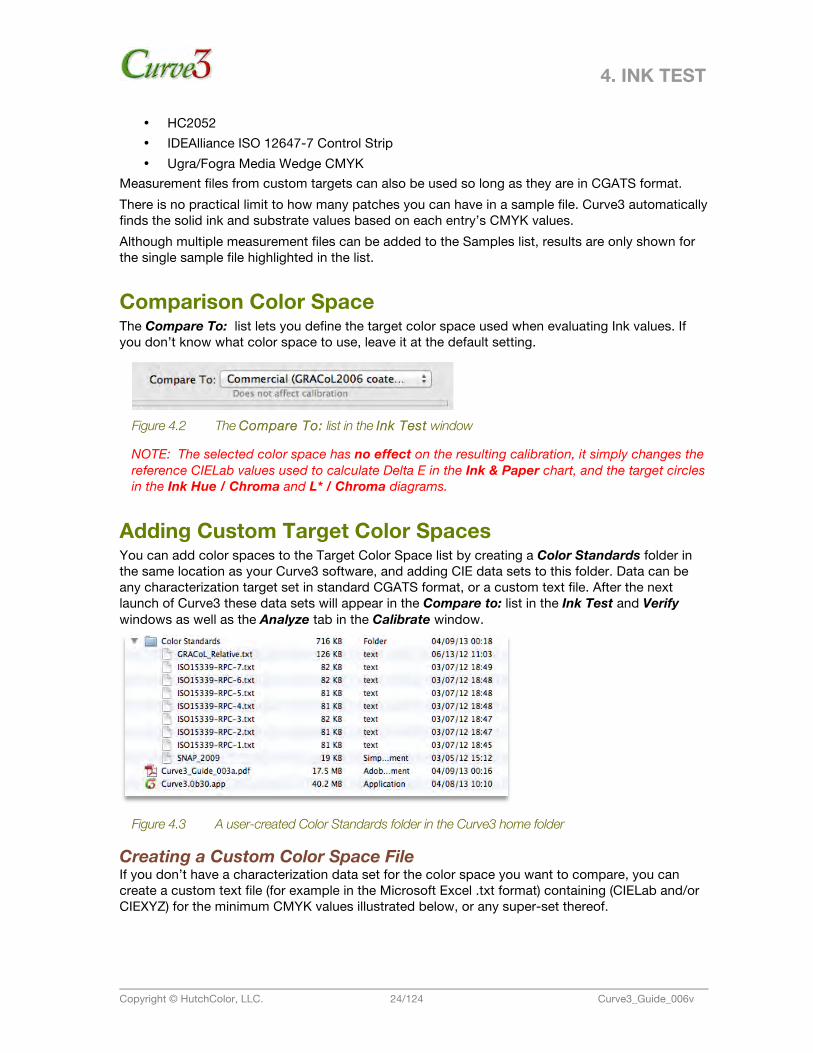
Comparison Color Space The Compare To: list lets you define the target color space used when evaluating Ink values. If you don’t know what color space to use, leave it at the default setting.
Figure 4.2 The Compare To: list in the Ink Test window
NOTE: The selected color space has no effect on the resulting calibration, it simply changes the reference CIELab values used to calculate Delta E in the Ink & Paper chart, and the target circles in the Ink Hue / Chroma and L* / Chroma diagrams.
Adding Custom Target Color Spaces You can add color spaces to the Target Color Space list by creating a Color Standards folder in the same location as your Curve3 software, and adding CIE data sets to this folder. Data can be any characterization target set in standard CGATS format, or a custom text file. After the next launch of Curve3 these data sets will appear in the Compare to: list in the Ink Test and Verify windows as well as the Analyze tab in the Calibrate window.
Figure 4.3 A user-created Color Standards folder in the Curve3 home folder
Creating a Custom Color Space File If you don’t have a characterization data set for the color space you want to compare, you can create a custom text file (for example in the Microsoft Excel .txt format) containing (CIELab and/or CIEXYZ) for the minimum CMYK values illustrated below, or any super-set thereof.
4. INK TEST
Copyright © HutchColor, LLC. 25/124 Curve3_Guide_006v
Figure 4.4 A minimal Target Color Space reference file recognized by Curve3
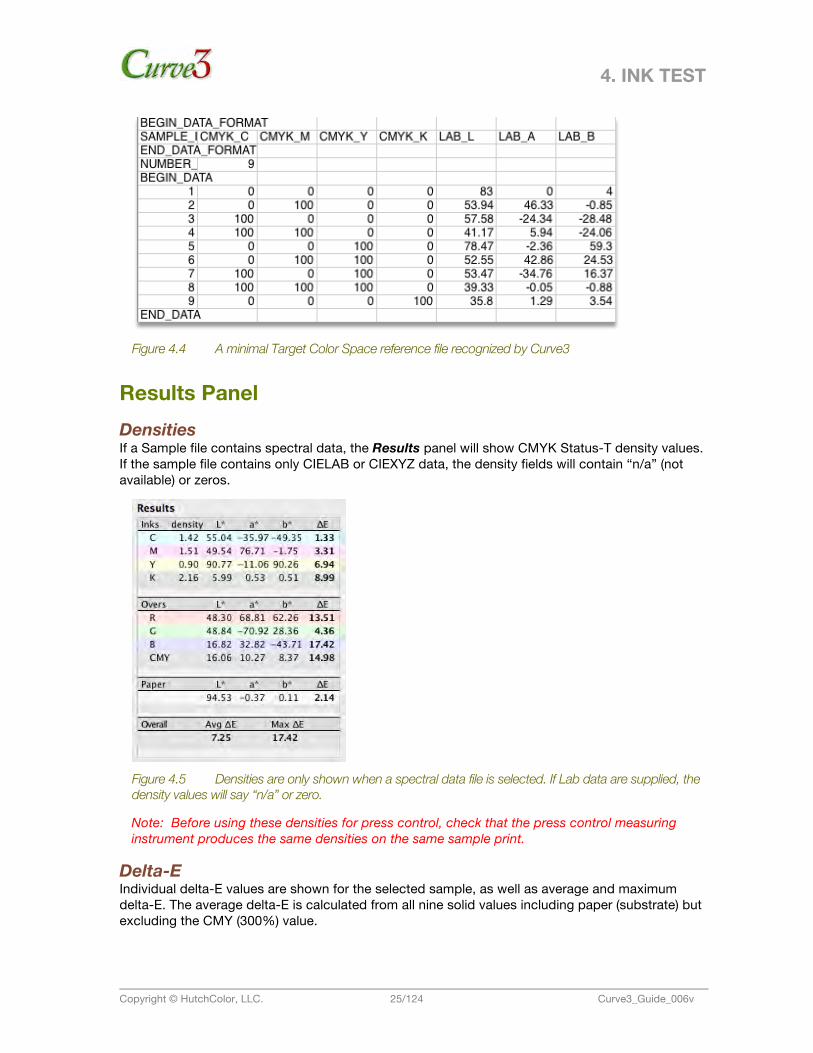
Results Panel Densities If a Sample file contains spectral data, the Results panel will show CMYK Status-T density values. If the sample file contains only CIELAB or CIEXYZ data, the density fields will contain “n/a” (not available) or zeros.
Figure 4.5 Densities are only shown when a spectral data file is selected. If Lab data are supplied, the density values will say “n/a” or zero.
Note: Before using these densities for press control, check that the press control measuring instrument produces the same densities on the same sample print.
Delta-E Individual delta-E values are shown for the selected sample, as well as average and maximum delta-E. The average delta-E is calculated from all nine solid values including paper (substrate) but excluding the CMY (300%) value.
4. INK TEST
Copyright © HutchColor, LLC. 26/124 Curve3_Guide_006v
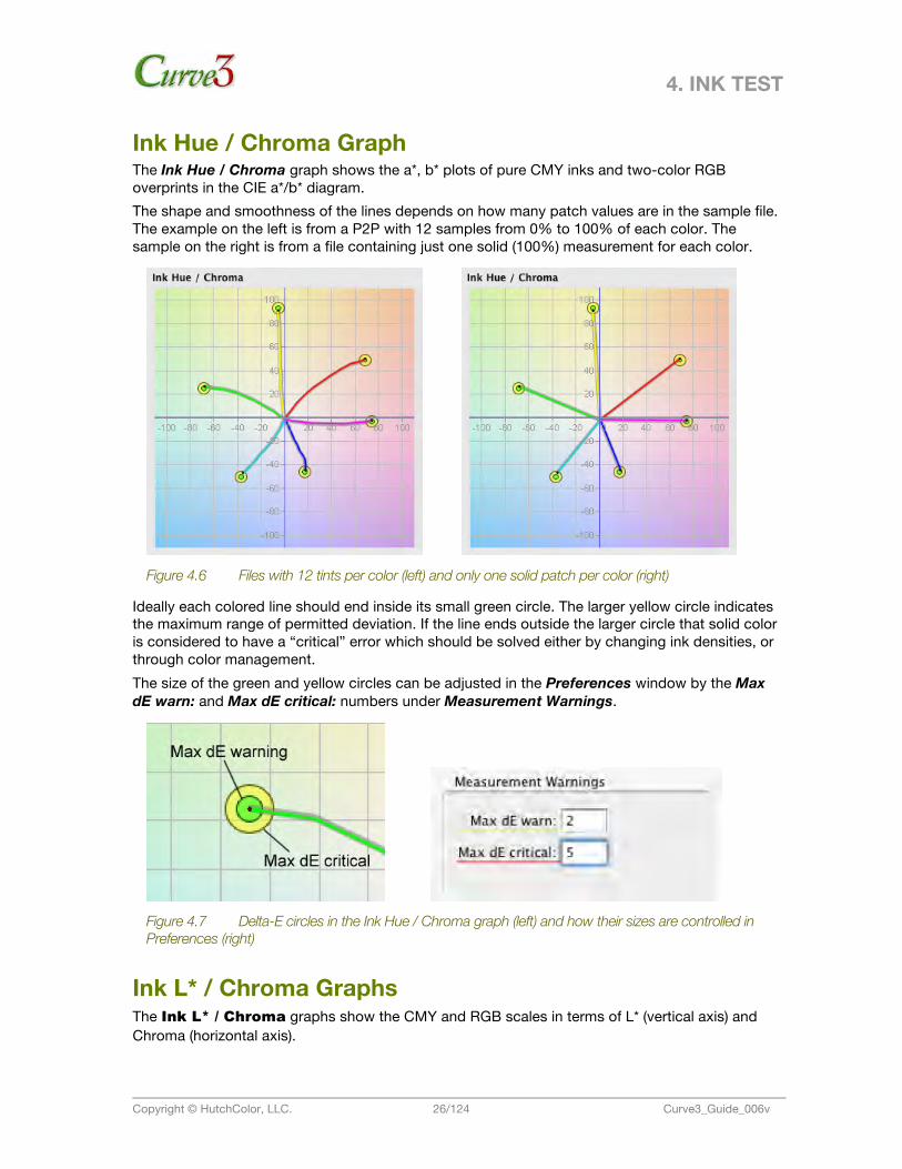
Ink Hue / Chroma Graph The Ink Hue / Chroma graph shows the a*, b* plots of pure CMY inks and two-color RGB overprints in the CIE a*/b* diagram. The shape and smoothness of the lines depends on how many patch values are in the sample file. The example on the left is from a P2P with 12 samples from 0% to 100% of each color. The sample on the right is from a file containing just one solid (100%) measurement for each color.
Figure 4.6 Files with 12 tints per color (left) and only one solid patch per color (right)
Ideally each colored line should end inside its small green circle. The larger yellow circle indicates the maximum range of permitted deviation. If the line ends outside the larger circle that solid color is considered to have a “critical” error which should be solved either by changing ink densities, or through color management. The size of the green and yellow circles can be adjusted in the Preferences window by the Max dE warn: and Max dE critical: numbers under Measurement Warnings.
Figure 4.7 Delta-E circles in the Ink Hue / Chroma graph (left) and how their sizes are controlled in Preferences (right)
Ink L* / Chroma Graphs The Ink L* / Chroma graphs show the CMY and RGB scales in terms of L* (vertical axis) and Chroma (horizontal axis).
4. INK TEST
Copyright © HutchColor, LLC. 27/124 Curve3_Guide_006v
Figure 4.8 The Ink L* / Chroma graphs alongside the Ink Hue / Chroma diagram
USER GUIDE
Copyright © HutchColor, LLC. 28/124 Curve3_Guide_006v
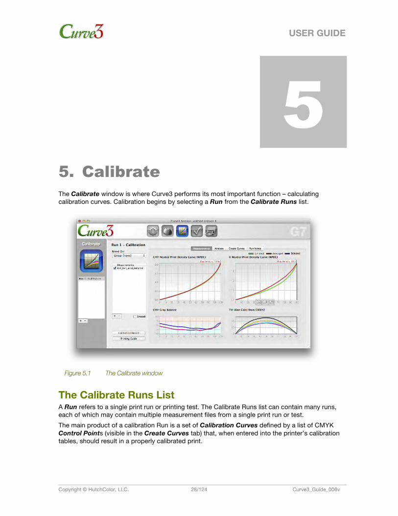
5. 5. Calibrate The Calibrate window is where Curve3 performs its most important function – calculating calibration curves. Calibration begins by selecting a Run from the Calibrate Runs list.
Figure 5.1 The Calibrate window
The Calibrate Runs List A Run refers to a single print run or printing test. The Calibrate Runs list can contain many runs, each of which may contain multiple measurement files from a single print run or test. The main product of a calibration Run is a set of Calibration Curves defined by a list of CMYK Control Points (visible in the Create Curves tab) that, when entered into the printer’s calibration tables, should result in a properly calibrated print.
5. CALIBRATE
Copyright © HutchColor, LLC. 29/124 Curve3_Guide_006v
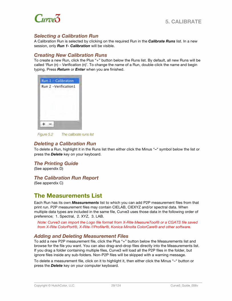
Selecting a Calibration Run A Calibration Run is selected by clicking on the required Run in the Calibrate Runs list. In a new session, only Run 1- Calibration will be visible.
Creating New Calibration Runs To create a new Run, click the Plus “+” button below the Runs list. By default, all new Runs will be called ‘Run (n) – Verification (n)’. To change the name of a Run, double-click the name and begin typing. Press Return or Enter when you are finished.
Figure 5.2 The calibrate runs list
Deleting a Calibration Run To delete a Run, highlight it in the Runs list then either click the Minus “–“ symbol below the list or press the Delete key on your keyboard.
The Printing Guide (See appendix D)
The Calibration Run Report (See appendix C)
The Measurements List Each Run has its own Measurements list to which you can add P2P measurement files from that print run. P2P measurement files may contain CIELAB, CIEXYZ and/or spectral data. When multiple data types are included in the same file, Curve3 uses those data in the following order of preference; 1. Spectral, 2. XYZ, 3. LAB.
Note: Curve3 can import the Logo file format from X-Rite MeasureTool® or a CGATS file saved from X-Rite ColorPort®, X-Rite i1Profiler®, Konica Minolta ColorCare® and other software.
Adding and Deleting Measurement Files To add a new P2P measurement file, click the Plus “+” button below the Measurements list and browse for the file you want. You can also drag-and-drop files directly into the Measurements list. If you drag a folder containing multiple files, Curve3 will load all the P2P files in the folder, but ignore files inside any sub-folders. Non-P2P files will be skipped with a warning message. To delete a measurement file, click on it to highlight it, then either click the Minus “–“ button or press the Delete key on your computer keyboard.
5. CALIBRATE
Copyright © HutchColor, LLC. 30/124 Curve3_Guide_006v
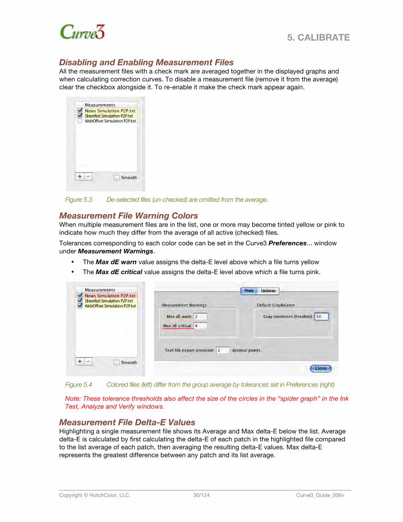
Disabling and Enabling Measurement Files All the measurement files with a check mark are averaged together in the displayed graphs and when calculating correction curves. To disable a measurement file (remove it from the average) clear the checkbox alongside it. To re-enable it make the check mark appear again.
Figure 5.3 De-selected files (un-checked) are omitted from the average.
Measurement File Warning Colors When multiple measurement files are in the list, one or more may become tinted yellow or pink to indicate how much they differ from the average of all active (checked) files. Tolerances corresponding to each color code can be set in the Curve3 Preferences... window under Measurement Warnings.
• The Max dE warn value assigns the delta-E level above which a file turns yellow • The Max dE critical value assigns the delta-E level above which a file turns pink.
Figure 5.4 Colored files (left) differ from the group average by tolerances set in Preferences (right)
Note: These tolerance thresholds also affect the size of the circles in the “spider graph” in the Ink Test, Analyze and Verify windows.
Measurement File Delta-E Values Highlighting a single measurement file shows its Average and Max delta-E below the list. Average delta-E is calculated by first calculating the delta-E of each patch in the highlighted file compared to the list average of each patch, then averaging the resulting delta-E values. Max delta-E represents the greatest difference between any patch and its list average.
5. CALIBRATE
Copyright © HutchColor, LLC. 31/124 Curve3_Guide_006v
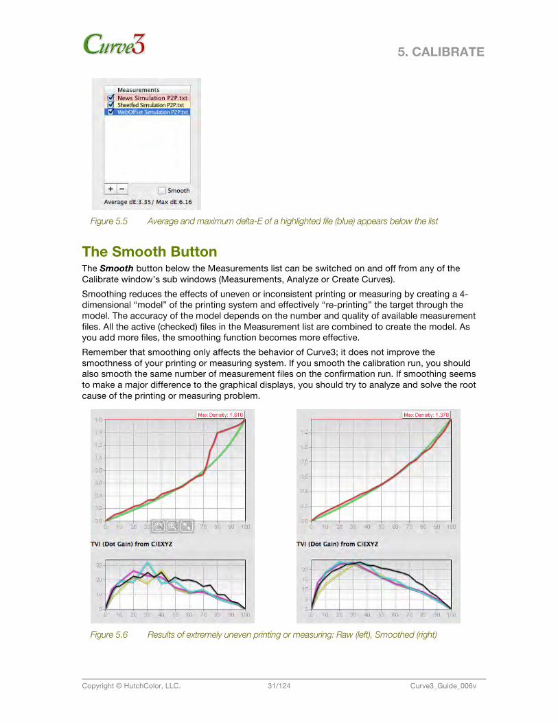
Figure 5.5 Average and maximum delta-E of a highlighted file (blue) appears below the list
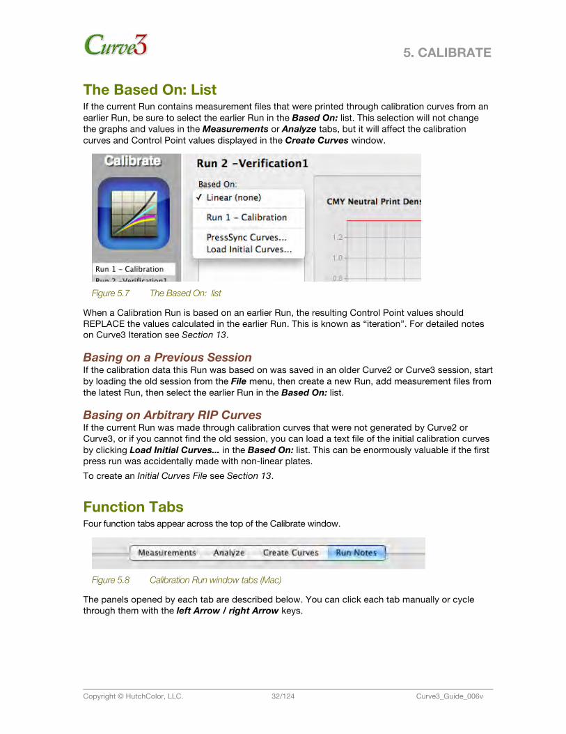
The Smooth Button The Smooth button below the Measurements list can be switched on and off from any of the Calibrate window’s sub windows (Measurements, Analyze or Create Curves). Smoothing reduces the effects of uneven or inconsistent printing or measuring by creating a 4-dimensional “model” of the printing system and effectively “re-printing” the target through the model. The accuracy of the model depends on the number and quality of available measurement files. All the active (checked) files in the Measurement list are combined to create the model. As you add more files, the smoothing function becomes more effective. Remember that smoothing only affects the behavior of Curve3; it does not improve the smoothness of your printing or measuring system. If you smooth the calibration run, you should also smooth the same number of measurement files on the confirmation run. If smoothing seems to make a major difference to the graphical displays, you should try to analyze and solve the root cause of the printing or measuring problem.
Figure 5.6 Results of extremely uneven printing or measuring: Raw (left), Smoothed (right)
5. CALIBRATE
Copyright © HutchColor, LLC. 32/124 Curve3_Guide_006v
The Based On: List If the current Run contains measurement files that were printed through calibration curves from an earlier Run, be sure to select the earlier Run in the Based On: list. This selection will not change the graphs and values in the Measurements or Analyze tabs, but it will affect the calibration curves and Control Point values displayed in the Create Curves window.
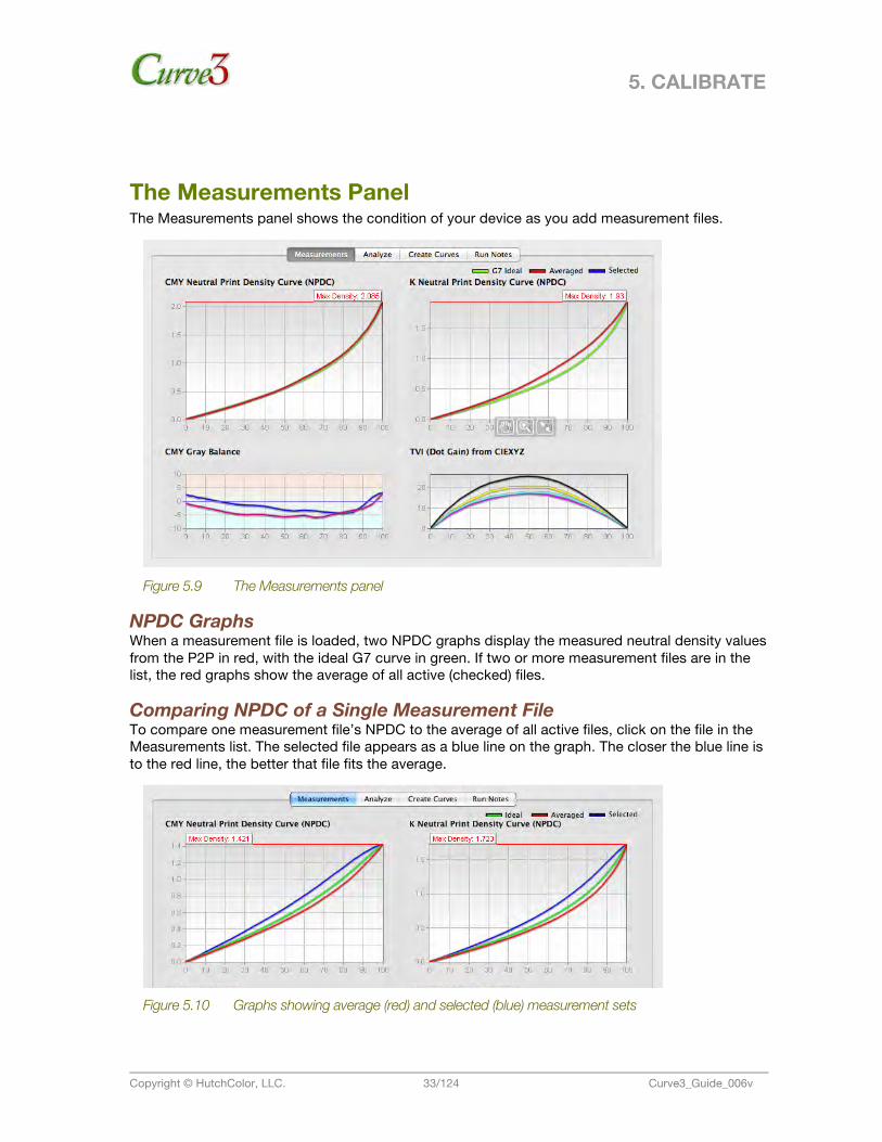
Figure 5.7 The Based On: list
When a Calibration Run is based on an earlier Run, the resulting Control Point values should REPLACE the values calculated in the earlier Run. This is known as “iteration”. For detailed notes on Curve3 Iteration see Section 13.
Basing on a Previous Session If the calibration data this Run was based on was saved in an older Curve2 or Curve3 session, start by loading the old session from the File menu, then create a new Run, add measurement files from the latest Run, then select the earlier Run in the Based On: list.
Basing on Arbitrary RIP Curves If the current Run was made through calibration curves that were not generated by Curve2 or Curve3, or if you cannot find the old session, you can load a text file of the initial calibration curves by clicking Load Initial Curves... in the Based On: list. This can be enormously valuable if the first press run was accidentally made with non-linear plates. To create an Initial Curves File see Section 13.
Function Tabs Four function tabs appear across the top of the Calibrate window.
Figure 5.8 Calibration Run window tabs (Mac)
The panels opened by each tab are described below. You can click each tab manually or cycle through them with the left Arrow / right Arrow keys.
5. CALIBRATE
Copyright © HutchColor, LLC. 33/124 Curve3_Guide_006v
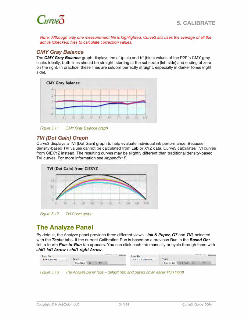
The Measurements Panel The Measurements panel shows the condition of your device as you add measurement files.
Figure 5.9 The Measurements panel
NPDC Graphs When a measurement file is loaded, two NPDC graphs display the measured neutral density values from the P2P in red, with the ideal G7 curve in green. If two or more measurement files are in the list, the red graphs show the average of all active (checked) files.
Comparing NPDC of a Single Measurement File To compare one measurement file’s NPDC to the average of all active files, click on the file in the Measurements list. The selected file appears as a blue line on the graph. The closer the blue line is to the red line, the better that file fits the average.
Figure 5.10 Graphs showing average (red) and selected (blue) measurement sets
5. CALIBRATE
Copyright © HutchColor, LLC. 34/124 Curve3_Guide_006v
Note: Although only one measurement file is highlighted, Curve3 still uses the average of all the active (checked) files to calculate correction values.
CMY Gray Balance The CMY Gray Balance graph displays the a* (pink) and b* (blue) values of the P2P’s CMY gray scale. Ideally, both lines should be straight, starting at the substrate (left side) and ending at zero on the right. In practice, these lines are seldom perfectly straight, especially in darker tones (right side).
Figure 5.11 CMY Gray Balance graph
TVI (Dot Gain) Graph Curve3 displays a TVI (Dot Gain) graph to help evaluate individual ink performance. Because density-based TVI values cannot be calculated from Lab or XYZ data, Curve3 calculates TVI curves from CIEXYZ instead. The resulting curves may be slightly different than traditional density-based TVI curves. For more information see Appendix: F.
Figure 5.12 TVI Curve graph
The Analyze Panel By default, the Analyze panel provides three different views - Ink & Paper, G7 and TVI, selected with the Tests: tabs. If the current Calibration Run is based on a previous Run in the Based On: list, a fourth Run-to-Run tab appears. You can click each tab manually or cycle through them with shift-left Arrow / shift-right Arrow.
Figure 5.13 The Analyze panel tabs – default (left) and based on an earlier Run (right)
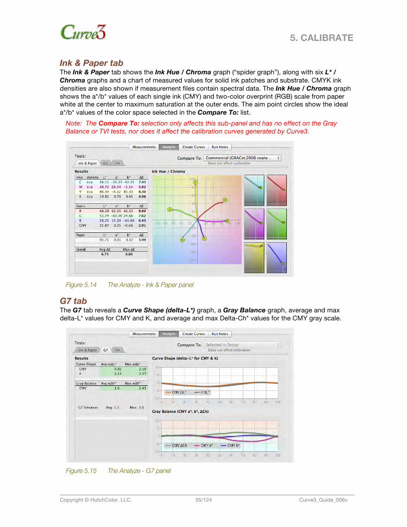
5. CALIBRATE
Copyright © HutchColor, LLC. 35/124 Curve3_Guide_006v
Ink & Paper tab The Ink & Paper tab shows the Ink Hue / Chroma graph (“spider graph”), along with six L* / Chroma graphs and a chart of measured values for solid ink patches and substrate. CMYK ink densities are also shown if measurement files contain spectral data. The Ink Hue / Chroma graph shows the a*/b* values of each single ink (CMY) and two-color overprint (RGB) scale from paper white at the center to maximum saturation at the outer ends. The aim point circles show the ideal a*/b* values of the color space selected in the Compare To: list.
Note: The Compare To: selection only affects this sub-panel and has no effect on the Gray Balance or TVI tests, nor does it affect the calibration curves generated by Curve3.
Figure 5.14 The Analyze - Ink & Paper panel
G7 tab The G7 tab reveals a Curve Shape (delta-L*) graph, a Gray Balance graph, average and max delta-L* values for CMY and K, and average and max Delta-Ch* values for the CMY gray scale.
Figure 5.15 The Analyze - G7 panel
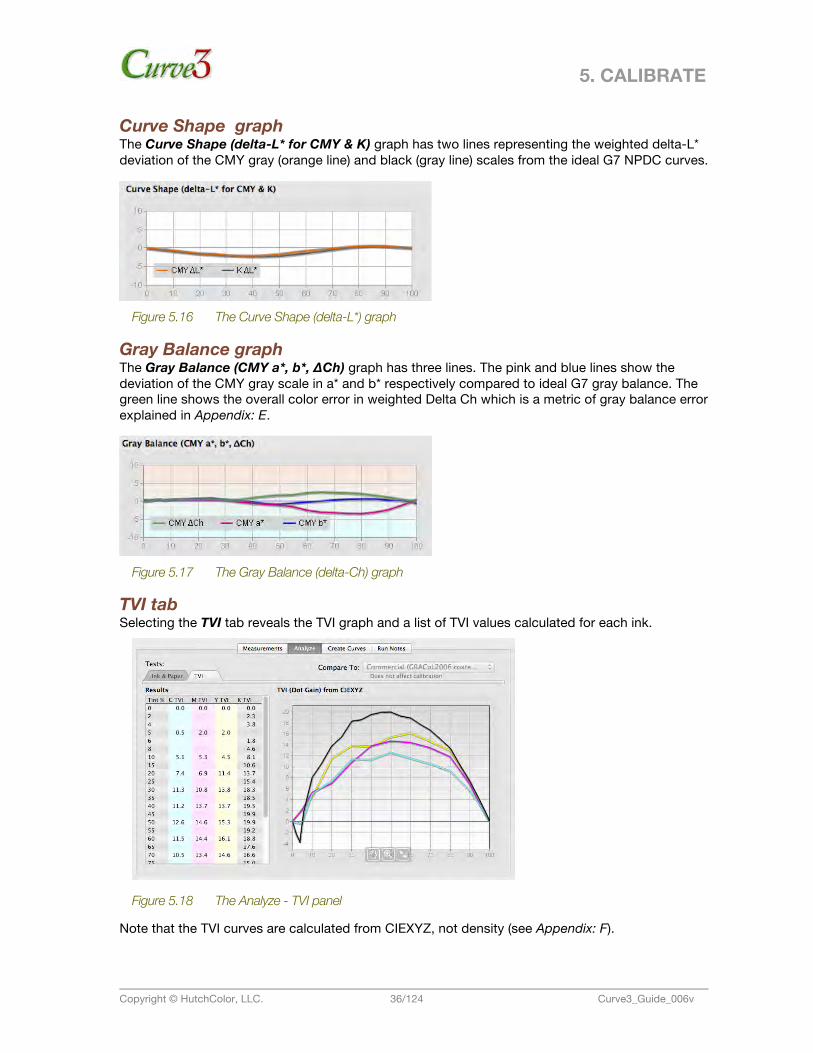
5. CALIBRATE
Copyright © HutchColor, LLC. 36/124 Curve3_Guide_006v
Curve Shape graph The Curve Shape (delta-L* for CMY & K) graph has two lines representing the weighted delta-L* deviation of the CMY gray (orange line) and black (gray line) scales from the ideal G7 NPDC curves.
Figure 5.16 The Curve Shape (delta-L*) graph
Gray Balance graph The Gray Balance (CMY a*, b*, ∆Ch) graph has three lines. The pink and blue lines show the deviation of the CMY gray scale in a* and b* respectively compared to ideal G7 gray balance. The green line shows the overall color error in weighted Delta Ch which is a metric of gray balance error explained in Appendix: E.
Figure 5.17 The Gray Balance (delta-Ch) graph
TVI tab Selecting the TVI tab reveals the TVI graph and a list of TVI values calculated for each ink.
Figure 5.18 The Analyze - TVI panel
Note that the TVI curves are calculated from CIEXYZ, not density (see Appendix: F).
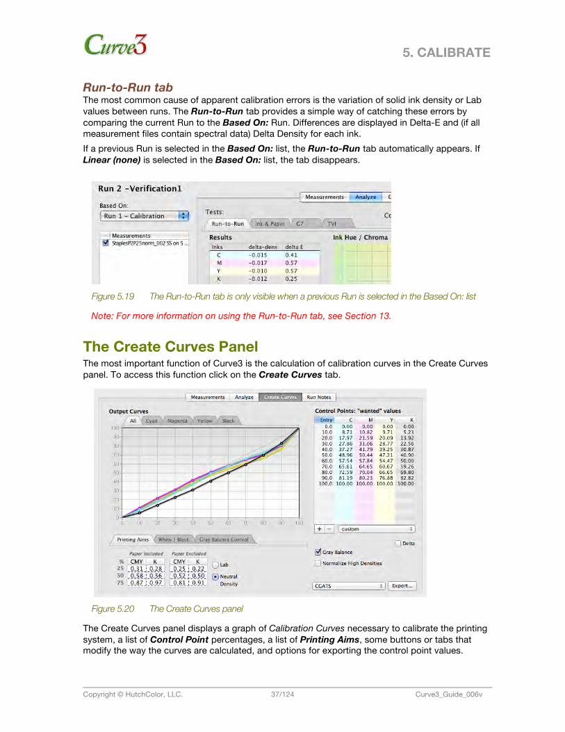
5. CALIBRATE
Copyright © HutchColor, LLC. 37/124 Curve3_Guide_006v
Run-to-Run tab The most common cause of apparent calibration errors is the variation of solid ink density or Lab values between runs. The Run-to-Run tab provides a simple way of catching these errors by comparing the current Run to the Based On: Run. Differences are displayed in Delta-E and (if all measurement files contain spectral data) Delta Density for each ink. If a previous Run is selected in the Based On: list, the Run-to-Run tab automatically appears. If Linear (none) is selected in the Based On: list, the tab disappears.
Figure 5.19 The Run-to-Run tab is only visible when a previous Run is selected in the Based On: list
Note: For more information on using the Run-to-Run tab, see Section 13.
The Create Curves Panel The most important function of Curve3 is the calculation of calibration curves in the Create Curves panel. To access this function click on the Create Curves tab.
Figure 5.20 The Create Curves panel
The Create Curves panel displays a graph of Calibration Curves necessary to calibrate the printing system, a list of Control Point percentages, a list of Printing Aims, some buttons or tabs that modify the way the curves are calculated, and options for exporting the control point values.
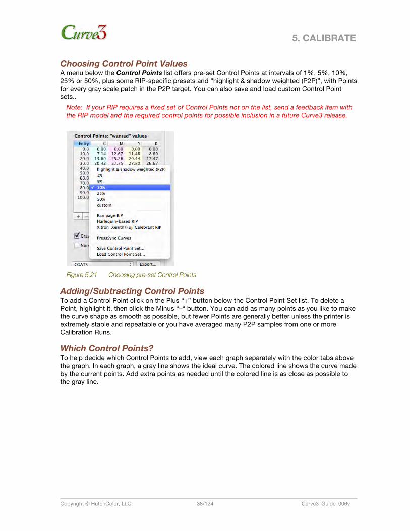
5. CALIBRATE
Copyright © HutchColor, LLC. 38/124 Curve3_Guide_006v
Choosing Control Point Values A menu below the Control Points list offers pre-set Control Points at intervals of 1%, 5%, 10%, 25% or 50%, plus some RIP-specific presets and “highlight & shadow weighted (P2P)”, with Points for every gray scale patch in the P2P target. You can also save and load custom Control Point sets..
Note: If your RIP requires a fixed set of Control Points not on the list, send a feedback item with the RIP model and the required control points for possible inclusion in a future Curve3 release.
Figure 5.21 Choosing pre-set Control Points
Adding/Subtracting Control Points To add a Control Point click on the Plus “+” button below the Control Point Set list. To delete a Point, highlight it, then click the Minus “–“ button. You can add as many points as you like to make the curve shape as smooth as possible, but fewer Points are generally better unless the printer is extremely stable and repeatable or you have averaged many P2P samples from one or more Calibration Runs.
Which Control Points? To help decide which Control Points to add, view each graph separately with the color tabs above the graph. In each graph, a gray line shows the ideal curve. The colored line shows the curve made by the current points. Add extra points as needed until the colored line is as close as possible to the gray line.
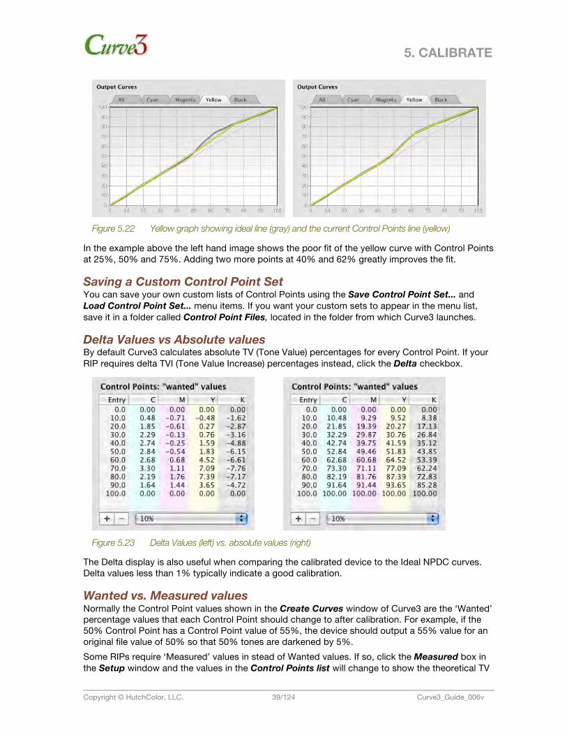
5. CALIBRATE
Copyright © HutchColor, LLC. 39/124 Curve3_Guide_006v
Figure 5.22 Yellow graph showing ideal line (gray) and the current Control Points line (yellow)
In the example above the left hand image shows the poor fit of the yellow curve with Control Points at 25%, 50% and 75%. Adding two more points at 40% and 62% greatly improves the fit.
Saving a Custom Control Point Set You can save your own custom lists of Control Points using the Save Control Point Set... and Load Control Point Set... menu items. If you want your custom sets to appear in the menu list, save it in a folder called Control Point Files, located in the folder from which Curve3 launches.
Delta Values vs Absolute values By default Curve3 calculates absolute TV (Tone Value) percentages for every Control Point. If your RIP requires delta TVI (Tone Value Increase) percentages instead, click the Delta checkbox.
Figure 5.23 Delta Values (left) vs. absolute values (right)
The Delta display is also useful when comparing the calibrated device to the Ideal NPDC curves. Delta values less than 1% typically indicate a good calibration.
Wanted vs. Measured values Normally the Control Point values shown in the Create Curves window of Curve3 are the ‘Wanted’ percentage values that each Control Point should change to after calibration. For example, if the 50% Control Point has a Control Point value of 55%, the device should output a 55% value for an original file value of 50% so that 50% tones are darkened by 5%. Some RIPs require ‘Measured’ values in stead of Wanted values. If so, click the Measured box in the Setup window and the values in the Control Points list will change to show the theoretical TV
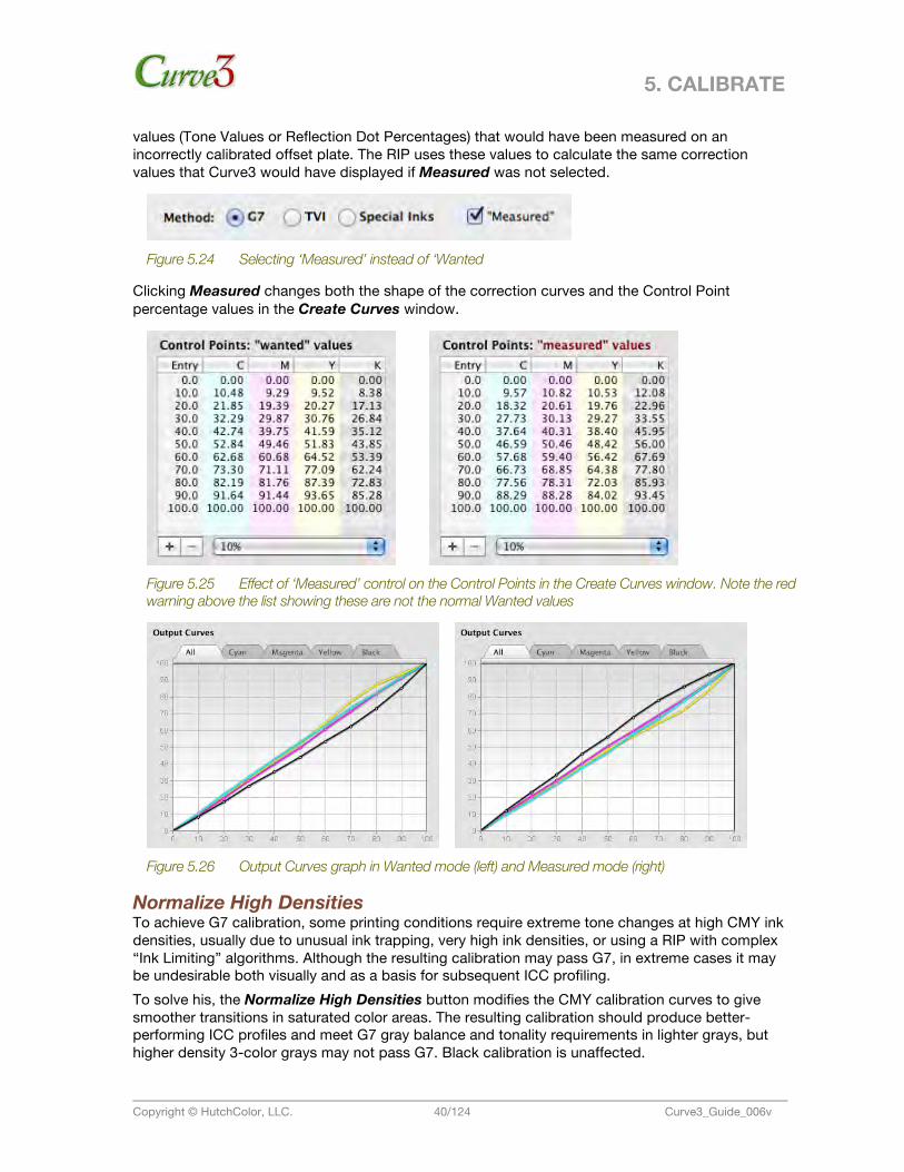
5. CALIBRATE
Copyright © HutchColor, LLC. 40/124 Curve3_Guide_006v
values (Tone Values or Reflection Dot Percentages) that would have been measured on an incorrectly calibrated offset plate. The RIP uses these values to calculate the same correction values that Curve3 would have displayed if Measured was not selected.
Figure 5.24 Selecting ‘Measured’ instead of ‘Wanted
Clicking Measured changes both the shape of the correction curves and the Control Point percentage values in the Create Curves window.
Figure 5.25 Effect of ‘Measured’ control on the Control Points in the Create Curves window. Note the red warning above the list showing these are not the normal Wanted values
Figure 5.26 Output Curves graph in Wanted mode (left) and Measured mode (right)
Normalize High Densities To achieve G7 calibration, some printing conditions require extreme tone changes at high CMY ink densities, usually due to unusual ink trapping, very high ink densities, or using a RIP with complex “Ink Limiting” algorithms. Although the resulting calibration may pass G7, in extreme cases it may be undesirable both visually and as a basis for subsequent ICC profiling. To solve his, the Normalize High Densities button modifies the CMY calibration curves to give smoother transitions in saturated color areas. The resulting calibration should produce better-performing ICC profiles and meet G7 gray balance and tonality requirements in lighter grays, but higher density 3-color grays may not pass G7. Black calibration is unaffected.
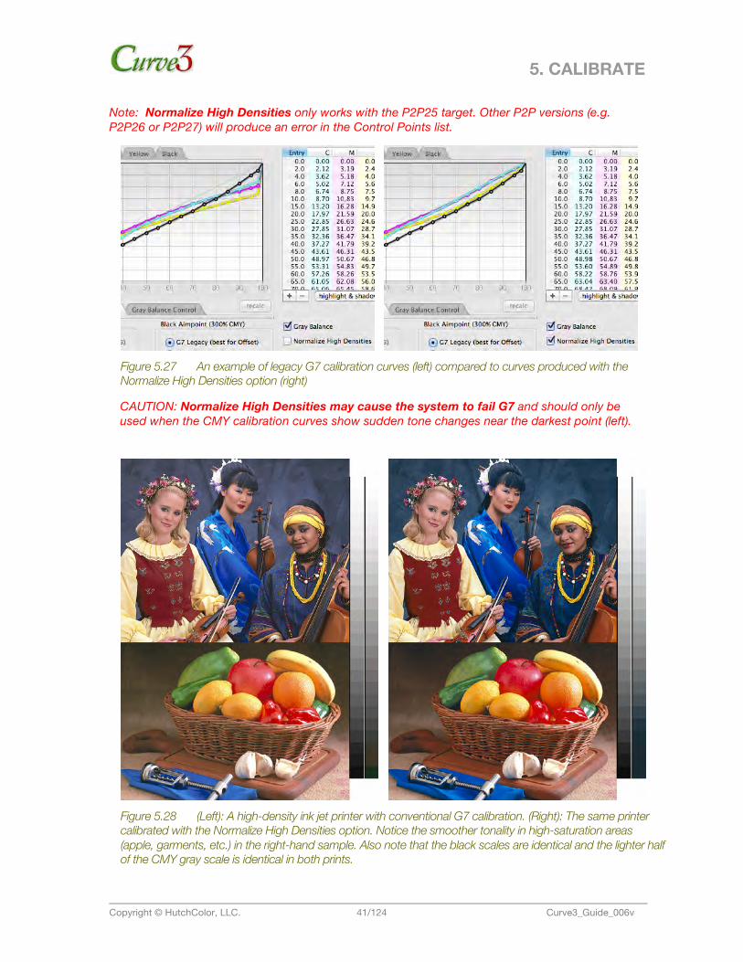
5. CALIBRATE
Copyright © HutchColor, LLC. 41/124 Curve3_Guide_006v
Note: Normalize High Densities only works with the P2P25 target. Other P2P versions (e.g. P2P26 or P2P27) will produce an error in the Control Points list.
Figure 5.27 An example of legacy G7 calibration curves (left) compared to curves produced with the Normalize High Densities option (right)
CAUTION: Normalize High Densities may cause the system to fail G7 and should only be used when the CMY calibration curves show sudden tone changes near the darkest point (left).
Figure 5.28 (Left): A high-density ink jet printer with conventional G7 calibration. (Right): The same printer calibrated with the Normalize High Densities option. Notice the smoother tonality in high-saturation areas (apple, garments, etc.) in the right-hand sample. Also note that the black scales are identical and the lighter half of the CMY gray scale is identical in both prints.
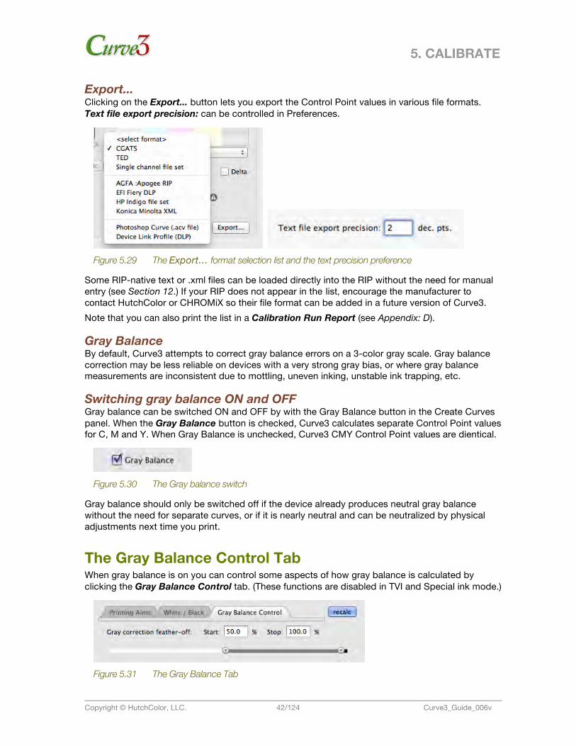
5. CALIBRATE
Copyright © HutchColor, LLC. 42/124 Curve3_Guide_006v
Export... Clicking on the Export... button lets you export the Control Point values in various file formats. Text file export precision: can be controlled in Preferences.
Figure 5.29 The Export... format selection list and the text precision preference
Some RIP-native text or .xml files can be loaded directly into the RIP without the need for manual entry (see Section 12.) If your RIP does not appear in the list, encourage the manufacturer to contact HutchColor or CHROMiX so their file format can be added in a future version of Curve3. Note that you can also print the list in a Calibration Run Report (see Appendix: D).
Gray Balance By default, Curve3 attempts to correct gray balance errors on a 3-color gray scale. Gray balance correction may be less reliable on devices with a very strong gray bias, or where gray balance measurements are inconsistent due to mottling, uneven inking, unstable ink trapping, etc.
Switching gray balance ON and OFF Gray balance can be switched ON and OFF by with the Gray Balance button in the Create Curves panel. When the Gray Balance button is checked, Curve3 calculates separate Control Point values for C, M and Y. When Gray Balance is unchecked, Curve3 CMY Control Point values are dientical.
Figure 5.30 The Gray balance switch
Gray balance should only be switched off if the device already produces neutral gray balance without the need for separate curves, or if it is nearly neutral and can be neutralized by physical adjustments next time you print.
The Gray Balance Control Tab When gray balance is on you can control some aspects of how gray balance is calculated by clicking the Gray Balance Control tab. (These functions are disabled in TVI and Special ink mode.)
Figure 5.31 The Gray Balance Tab
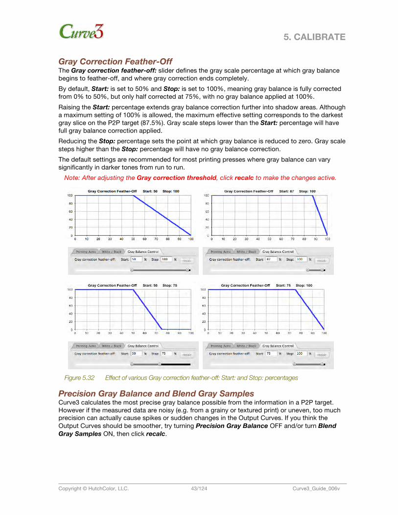
5. CALIBRATE
Copyright © HutchColor, LLC. 43/124 Curve3_Guide_006v
Gray Correction Feather-Off The Gray correction feather-off: slider defines the gray scale percentage at which gray balance begins to feather-off, and where gray correction ends completely. By default, Start: is set to 50% and Stop: is set to 100%, meaning gray balance is fully corrected from 0% to 50%, but only half corrected at 75%, with no gray balance applied at 100%. Raising the Start: percentage extends gray balance correction further into shadow areas. Although a maximum setting of 100% is allowed, the maximum effective setting corresponds to the darkest gray slice on the P2P target (87.5%). Gray scale steps lower than the Start: percentage will have full gray balance correction applied. Reducing the Stop: percentage sets the point at which gray balance is reduced to zero. Gray scale steps higher than the Stop: percentage will have no gray balance correction. The default settings are recommended for most printing presses where gray balance can vary significantly in darker tones from run to run.
Note: After adjusting the Gray correction threshold, click recalc to make the changes active.
Figure 5.32 Effect of various Gray correction feather-off: Start: and Stop: percentages
Precision Gray Balance and Blend Gray Samples Curve3 calculates the most precise gray balance possible from the information in a P2P target. However if the measured data are noisy (e.g. from a grainy or textured print) or uneven, too much precision can actually cause spikes or sudden changes in the Output Curves. If you think the Output Curves should be smoother, try turning Precision Gray Balance OFF and/or turn Blend Gray Samples ON, then click recalc.
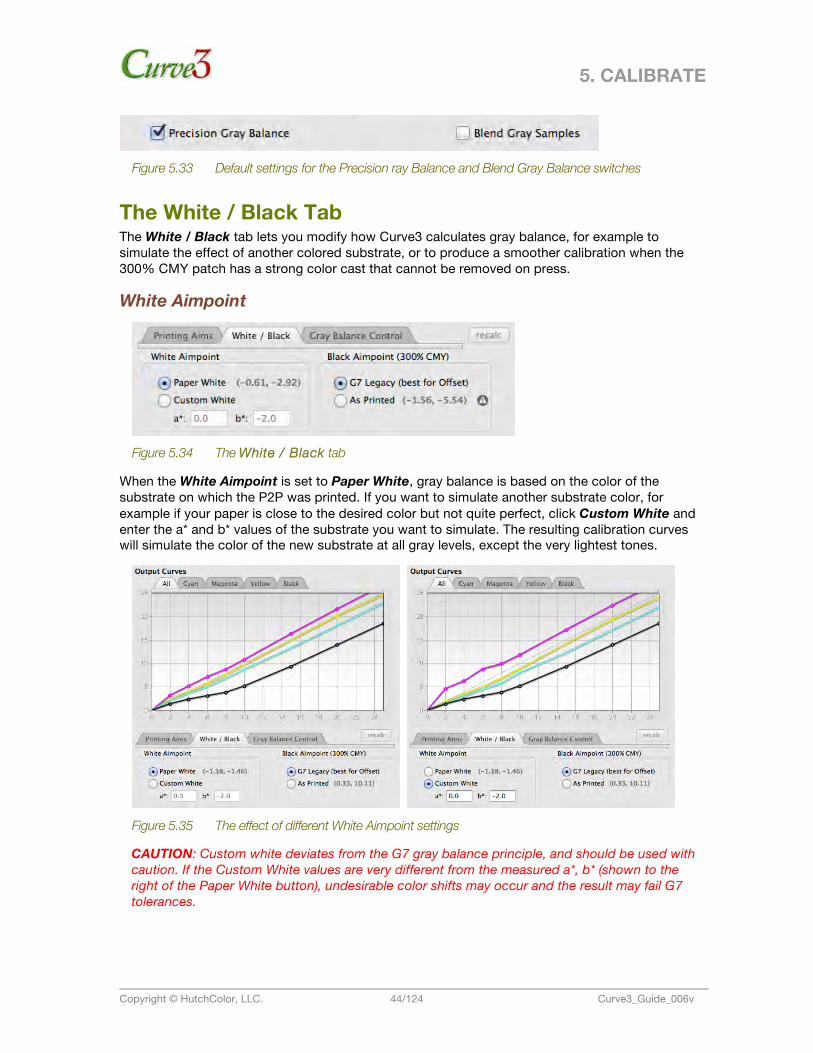
5. CALIBRATE
Copyright © HutchColor, LLC. 44/124 Curve3_Guide_006v
Figure 5.33 Default settings for the Precision ray Balance and Blend Gray Balance switches
The White / Black Tab The White / Black tab lets you modify how Curve3 calculates gray balance, for example to simulate the effect of another colored substrate, or to produce a smoother calibration when the 300% CMY patch has a strong color cast that cannot be removed on press.
White Aimpoint
Figure 5.34 The White / Black tab
When the White Aimpoint is set to Paper White, gray balance is based on the color of the substrate on which the P2P was printed. If you want to simulate another substrate color, for example if your paper is close to the desired color but not quite perfect, click Custom White and enter the a* and b* values of the substrate you want to simulate. The resulting calibration curves will simulate the color of the new substrate at all gray levels, except the very lightest tones.
Figure 5.35 The effect of different White Aimpoint settings
CAUTION: Custom white deviates from the G7 gray balance principle, and should be used with caution. If the Custom White values are very different from the measured a*, b* (shown to the right of the Paper White button), undesirable color shifts may occur and the result may fail G7 tolerances.
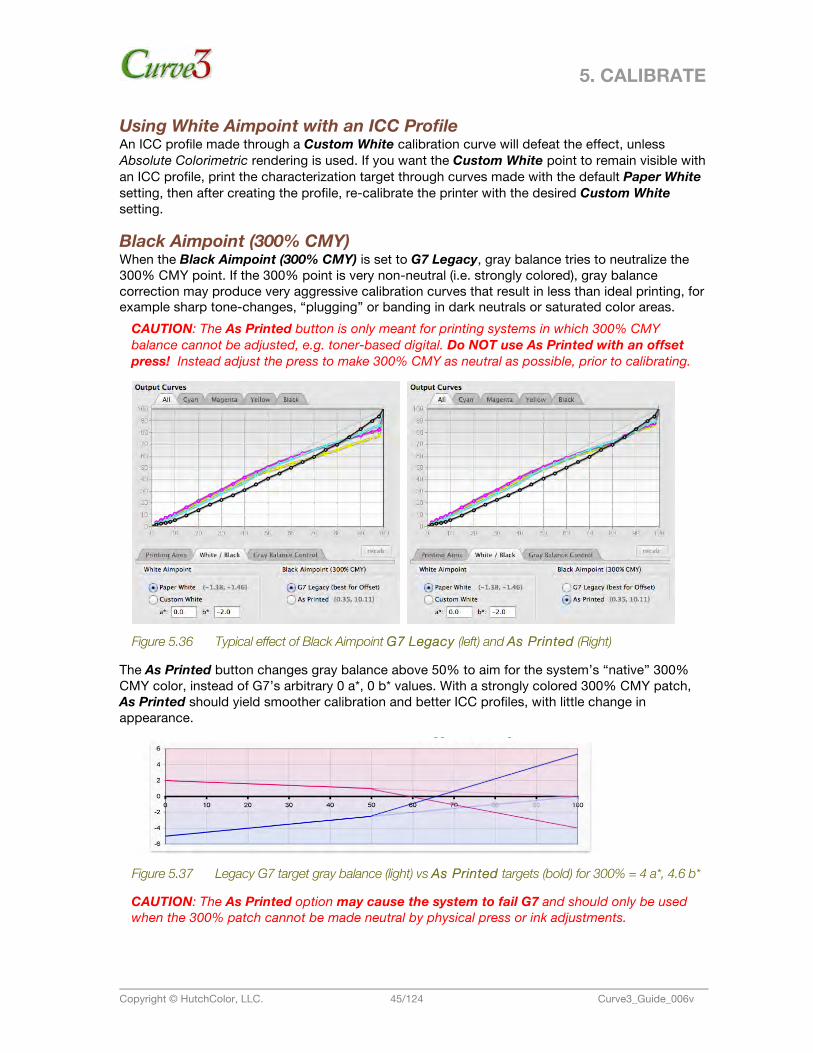
5. CALIBRATE
Copyright © HutchColor, LLC. 45/124 Curve3_Guide_006v
Using White Aimpoint with an ICC Profile An ICC profile made through a Custom White calibration curve will defeat the effect, unless Absolute Colorimetric rendering is used. If you want the Custom White point to remain visible with an ICC profile, print the characterization target through curves made with the default Paper White setting, then after creating the profile, re-calibrate the printer with the desired Custom White setting.
Black Aimpoint (300% CMY) When the Black Aimpoint (300% CMY) is set to G7 Legacy, gray balance tries to neutralize the 300% CMY point. If the 300% point is very non-neutral (i.e. strongly colored), gray balance correction may produce very aggressive calibration curves that result in less than ideal printing, for example sharp tone-changes, “plugging” or banding in dark neutrals or saturated color areas.
CAUTION: The As Printed button is only meant for printing systems in which 300% CMY balance cannot be adjusted, e.g. toner-based digital. Do NOT use As Printed with an offset press! Instead adjust the press to make 300% CMY as neutral as possible, prior to calibrating.
Figure 5.36 Typical effect of Black Aimpoint G7 Legacy (left) and As Printed (Right)
The As Printed button changes gray balance above 50% to aim for the system’s “native” 300% CMY color, instead of G7’s arbitrary 0 a*, 0 b* values. With a strongly colored 300% CMY patch, As Printed should yield smoother calibration and better ICC profiles, with little change in appearance.
Figure 5.37 Legacy G7 target gray balance (light) vs As Printed targets (bold) for 300% = 4 a*, 4.6 b*
CAUTION: The As Printed option may cause the system to fail G7 and should only be used when the 300% patch cannot be made neutral by physical press or ink adjustments.
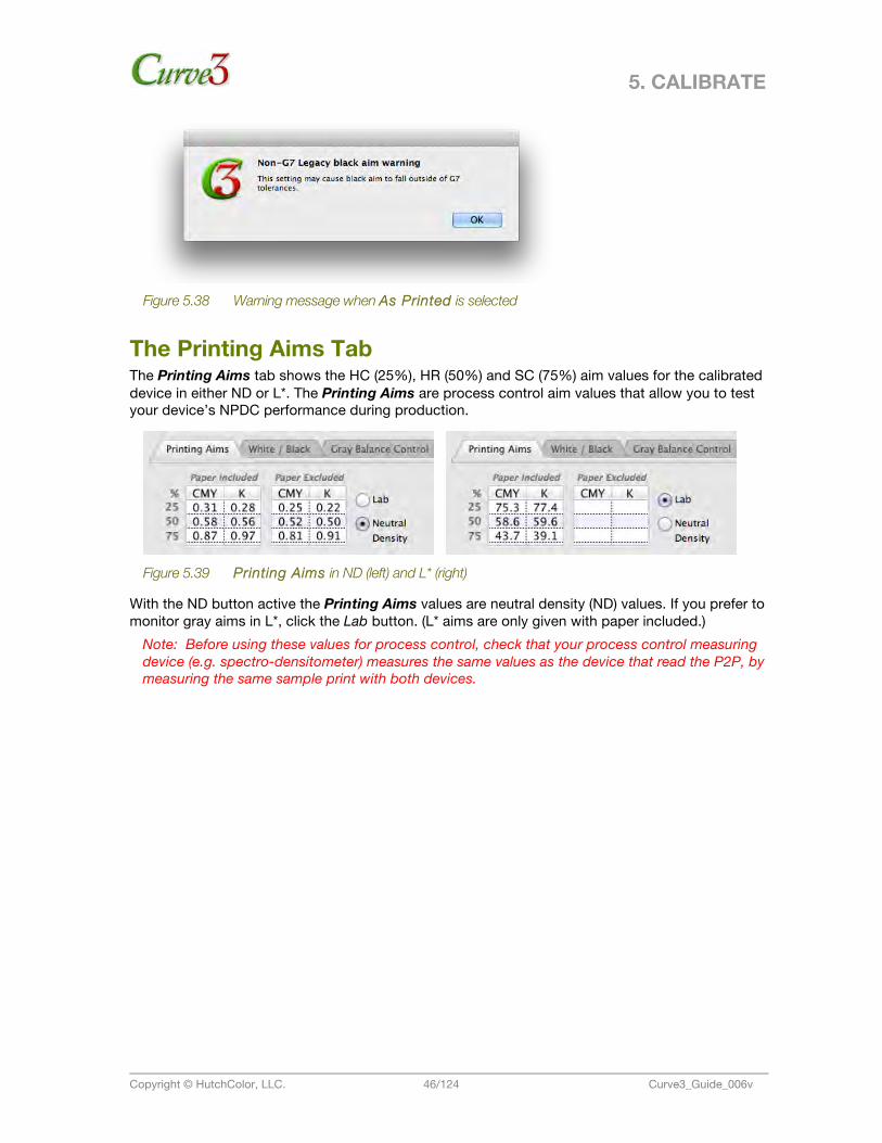
5. CALIBRATE
Copyright © HutchColor, LLC. 46/124 Curve3_Guide_006v
Figure 5.38 Warning message when As Printed is selected
The Printing Aims Tab The Printing Aims tab shows the HC (25%), HR (50%) and SC (75%) aim values for the calibrated device in either ND or L*. The Printing Aims are process control aim values that allow you to test your device’s NPDC performance during production.
Figure 5.39 Printing Aims in ND (left) and L* (right)
With the ND button active the Printing Aims values are neutral density (ND) values. If you prefer to monitor gray aims in L*, click the Lab button. (L* aims are only given with paper included.)
Note: Before using these values for process control, check that your process control measuring device (e.g. spectro-densitometer) measures the same values as the device that read the P2P, by measuring the same sample print with both devices.
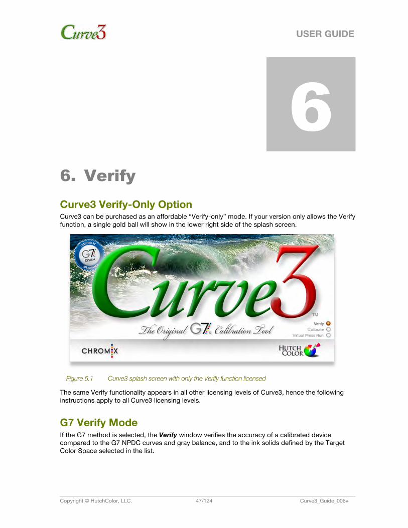
USER GUIDE
Copyright © HutchColor, LLC. 47/124 Curve3_Guide_006v
6. 6. Verify Curve3 Verify-Only Option Curve3 can be purchased as an affordable “Verify-only” mode. If your version only allows the Verify function, a single gold ball will show in the lower right side of the splash screen.
Figure 6.1 Curve3 splash screen with only the Verify function licensed
The same Verify functionality appears in all other licensing levels of Curve3, hence the following instructions apply to all Curve3 licensing levels.
G7 Verify Mode If the G7 method is selected, the Verify window verifies the accuracy of a calibrated device compared to the G7 NPDC curves and gray balance, and to the ink solids defined by the Target Color Space selected in the list.
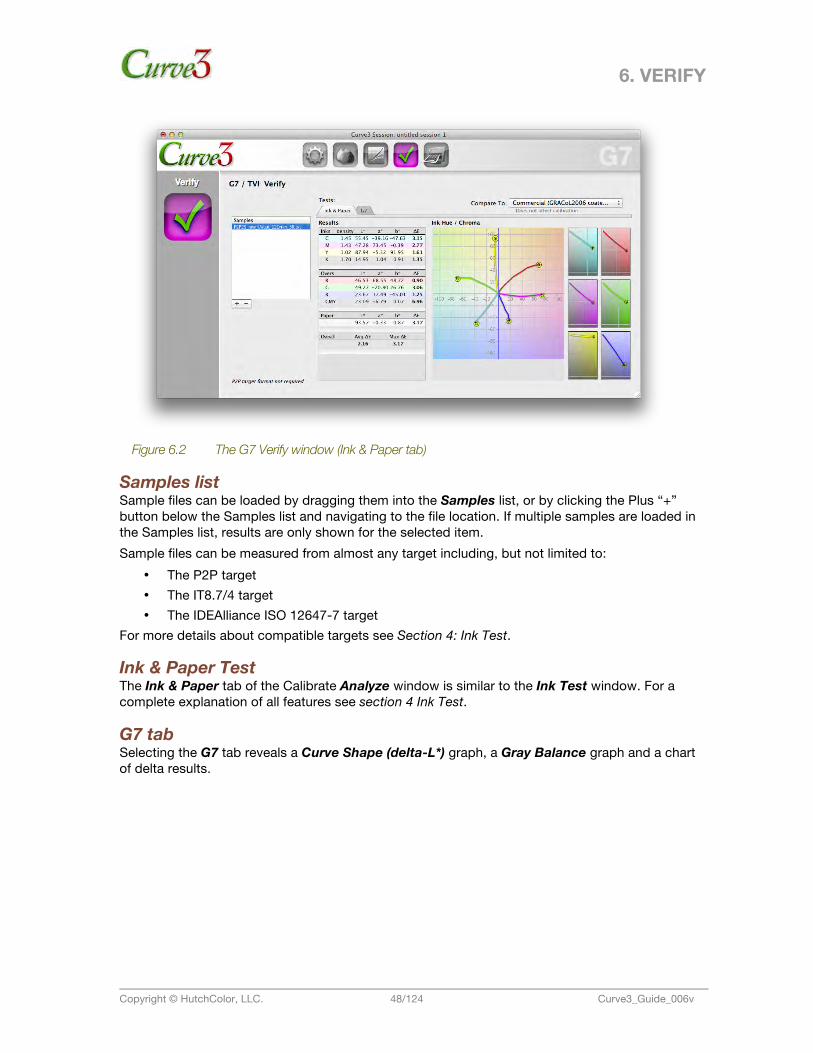
6. VERIFY
Copyright © HutchColor, LLC. 48/124 Curve3_Guide_006v
Figure 6.2 The G7 Verify window (Ink & Paper tab)
Samples list Sample files can be loaded by dragging them into the Samples list, or by clicking the Plus “+” button below the Samples list and navigating to the file location. If multiple samples are loaded in the Samples list, results are only shown for the selected item. Sample files can be measured from almost any target including, but not limited to:
• The P2P target • The IT8.7/4 target • The IDEAlliance ISO 12647-7 target
For more details about compatible targets see Section 4: Ink Test.
Ink & Paper Test The Ink & Paper tab of the Calibrate Analyze window is similar to the Ink Test window. For a complete explanation of all features see section 4 Ink Test.
G7 tab Selecting the G7 tab reveals a Curve Shape (delta-L*) graph, a Gray Balance graph and a chart of delta results.
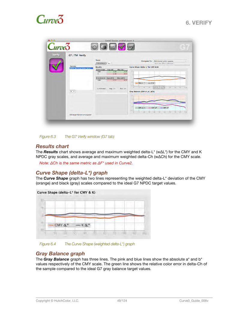
6. VERIFY
Copyright © HutchColor, LLC. 49/124 Curve3_Guide_006v
Figure 6.3 The G7 Verify window (G7 tab)
Results chart The Results chart shows average and maximum weighted delta-L* (w∆L*) for the CMY and K NPDC gray scales, and average and maximum weighted delta-Ch (w∆Ch) for the CMY scale.
Note: ∆Ch is the same metric as ∆F* used in Curve2.
Curve Shape (delta-L*) graph The Curve Shape graph has two lines representing the weighted delta-L* deviation of the CMY (orange) and black (gray) scales compared to the ideal G7 NPDC target values.
Figure 6.4 The Curve Shape (weighted delta-L*) graph
Gray Balance graph The Gray Balance graph has three lines. The pink and blue lines show the absolute a* and b* values respectively of the CMY scale. The green line shows the relative color error in delta-Ch of the sample compared to the ideal G7 gray balance target values.
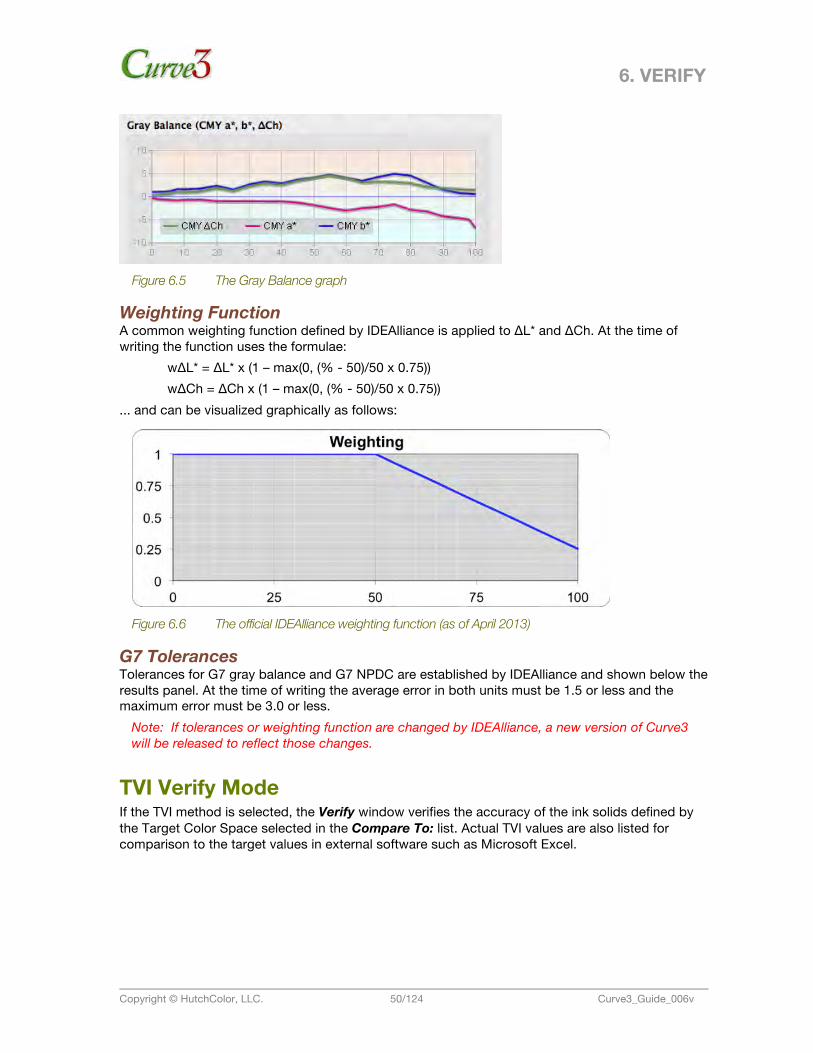
6. VERIFY
Copyright © HutchColor, LLC. 50/124 Curve3_Guide_006v
Figure 6.5 The Gray Balance graph
Weighting Function A common weighting function defined by IDEAlliance is applied to ∆L* and ∆Ch. At the time of writing the function uses the formulae:
w∆L* = ∆L* x (1 – max(0, (% - 50)/50 x 0.75)) w∆Ch = ∆Ch x (1 – max(0, (% - 50)/50 x 0.75))
... and can be visualized graphically as follows:
Figure 6.6 The official IDEAlliance weighting function (as of April 2013)
G7 Tolerances Tolerances for G7 gray balance and G7 NPDC are established by IDEAlliance and shown below the results panel. At the time of writing the average error in both units must be 1.5 or less and the maximum error must be 3.0 or less.
Note: If tolerances or weighting function are changed by IDEAlliance, a new version of Curve3 will be released to reflect those changes.
TVI Verify Mode If the TVI method is selected, the Verify window verifies the accuracy of the ink solids defined by the Target Color Space selected in the Compare To: list. Actual TVI values are also listed for comparison to the target values in external software such as Microsoft Excel.
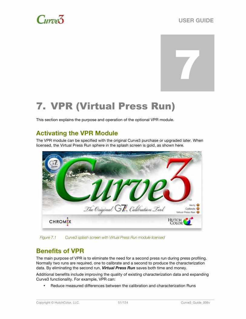
USER GUIDE
Copyright © HutchColor, LLC. 51/124 Curve3_Guide_006v
7. 7. VPR (Virtual Press Run) This section explains the purpose and operation of the optional VPR module.
Activating the VPR Module The VPR module can be specified with the original Curve3 purchase or upgraded later. When licensed, the Virtual Press Run sphere in the splash screen is gold, as shown here.
Figure 7.1 Curve3 splash screen with Virtual Press Run module licensed
Benefits of VPR The main purpose of VPR is to eliminate the need for a second press run during press profiling. Normally two runs are required, one to calibrate and a second to produce the characterization data. By eliminating the second run, Virtual Press Run saves both time and money. Additional benefits include improving the quality of existing characterization data and expanding Curve3 functionality. For example, VPR can:
• Reduce measured differences between the calibration and characterization Runs
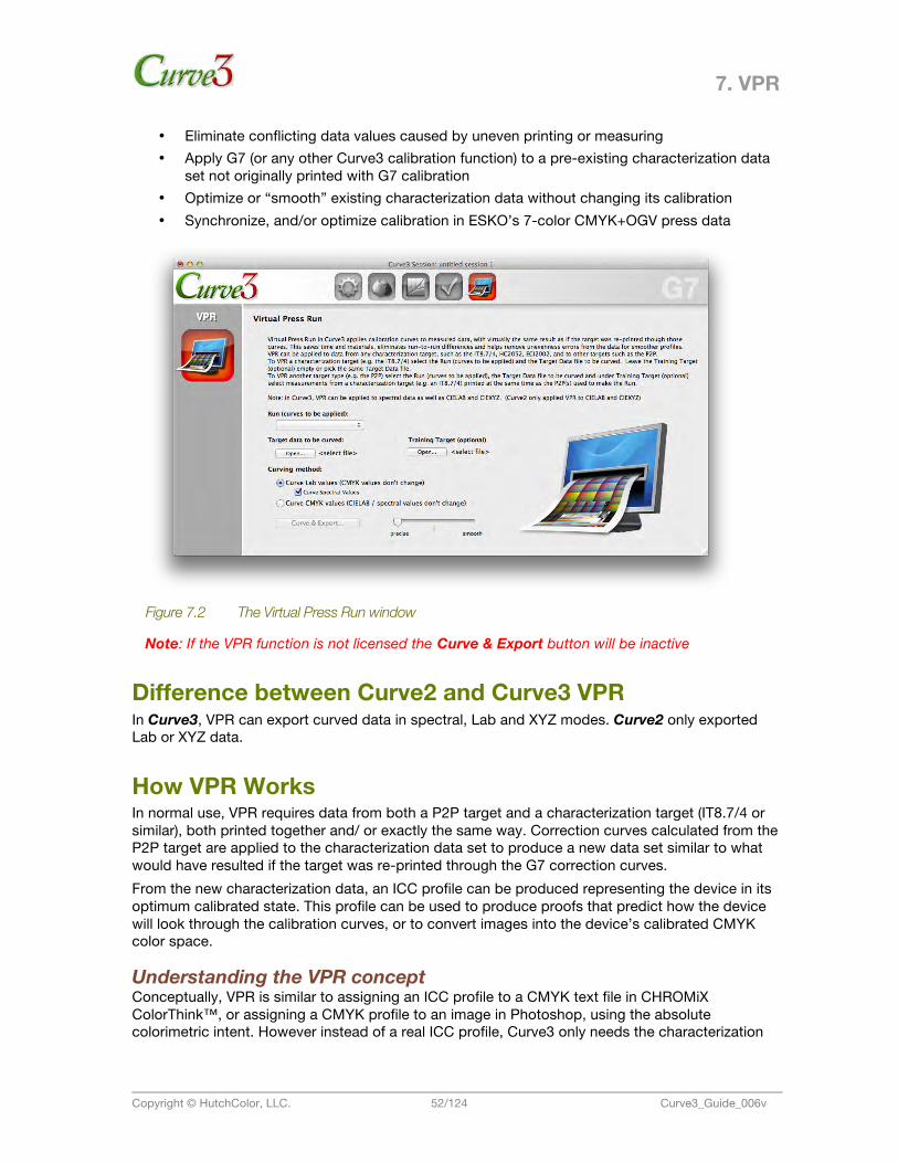
7. VPR
Copyright © HutchColor, LLC. 52/124 Curve3_Guide_006v
• Eliminate conflicting data values caused by uneven printing or measuring • Apply G7 (or any other Curve3 calibration function) to a pre-existing characterization data
set not originally printed with G7 calibration • Optimize or “smooth” existing characterization data without changing its calibration • Synchronize, and/or optimize calibration in ESKO’s 7-color CMYK+OGV press data
Figure 7.2 The Virtual Press Run window
Note: If the VPR function is not licensed the Curve & Export button will be inactive
Difference between Curve2 and Curve3 VPR In Curve3, VPR can export curved data in spectral, Lab and XYZ modes. Curve2 only exported Lab or XYZ data.
How VPR Works In normal use, VPR requires data from both a P2P target and a characterization target (IT8.7/4 or similar), both printed together and/ or exactly the same way. Correction curves calculated from the P2P target are applied to the characterization data set to produce a new data set similar to what would have resulted if the target was re-printed through the G7 correction curves. From the new characterization data, an ICC profile can be produced representing the device in its optimum calibrated state. This profile can be used to produce proofs that predict how the device will look through the calibration curves, or to convert images into the device’s calibrated CMYK color space.
Understanding the VPR concept Conceptually, VPR is similar to assigning an ICC profile to a CMYK text file in CHROMiX ColorThink™, or assigning a CMYK profile to an image in Photoshop, using the absolute colorimetric intent. However instead of a real ICC profile, Curve3 only needs the characterization
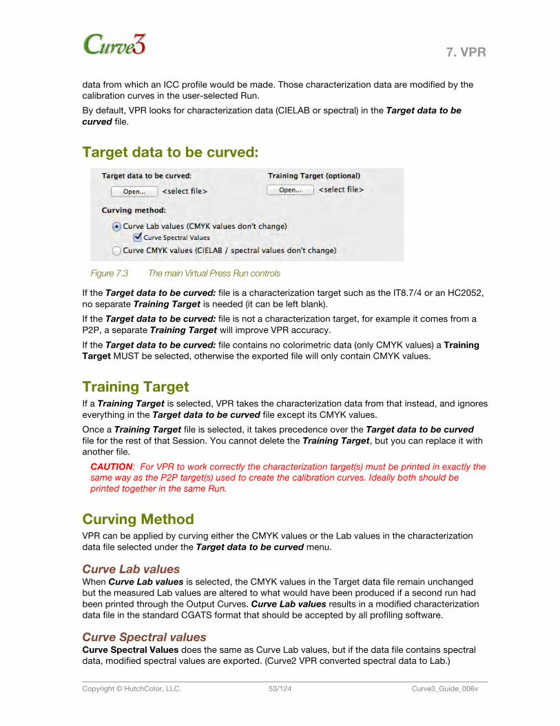
7. VPR
Copyright © HutchColor, LLC. 53/124 Curve3_Guide_006v
data from which an ICC profile would be made. Those characterization data are modified by the calibration curves in the user-selected Run. By default, VPR looks for characterization data (CIELAB or spectral) in the Target data to be curved file.
Target data to be curved:
Figure 7.3 The main Virtual Press Run controls
If the Target data to be curved: file is a characterization target such as the IT8.7/4 or an HC2052, no separate Training Target is needed (it can be left blank). If the Target data to be curved: file is not a characterization target, for example it comes from a P2P, a separate Training Target will improve VPR accuracy. If the Target data to be curved: file contains no colorimetric data (only CMYK values) a Training Target MUST be selected, otherwise the exported file will only contain CMYK values.
Training Target If a Training Target is selected, VPR takes the characterization data from that instead, and ignores everything in the Target data to be curved file except its CMYK values. Once a Training Target file is selected, it takes precedence over the Target data to be curved file for the rest of that Session. You cannot delete the Training Target, but you can replace it with another file.
CAUTION: For VPR to work correctly the characterization target(s) must be printed in exactly the same way as the P2P target(s) used to create the calibration curves. Ideally both should be printed together in the same Run.
Curving Method VPR can be applied by curving either the CMYK values or the Lab values in the characterization data file selected under the Target data to be curved menu.
Curve Lab values When Curve Lab values is selected, the CMYK values in the Target data file remain unchanged but the measured Lab values are altered to what would have been produced if a second run had been printed through the Output Curves. Curve Lab values results in a modified characterization data file in the standard CGATS format that should be accepted by all profiling software.
Curve Spectral values Curve Spectral Values does the same as Curve Lab values, but if the data file contains spectral data, modified spectral values are exported. (Curve2 VPR converted spectral data to Lab.)
7. VPR
Copyright © HutchColor, LLC. 54/124 Curve3_Guide_006v
Curve CMYK values When Curve CMYK values is selected, the Lab values measured from the printed Target are unchanged but the CMYK values are altered by the Output Curves in the selected Run. Curve CMYK values results in non-standard CMYK values which may not work in some profiling software, hence Curve Lab Values... is the default option.
Applying VPR to a Characterization Target VPR can be applied to data measured from a characterization target such as the IT8.7/4 or HC2052, or any custom characterization target saved in the CGATS file format. To apply VPR to a characterization target:
• Select the curves you want to apply from the Run (Curves to be Applied) list • Select the Target data file with the Target data to be curved button • Select the Curving method (normally Curve Lab values) • Set the Quality slider (normally “precise” is best) • Click Curve & Export and save the new characterization data file in a suitable location
Applying VPR to Non-Characterization Data VPR can be applied not just to a characterization target, but to any data file, such as the P2P or the IDEAlliance ISO 12647-7 Control Target. Using the Curve Lab values option, best results will be had by selecting a characterization target in the Training target list from the same run. Using the Curve CMYK option, no training target is needed. To apply VPR to a non-characterization target:
• Select the curves you want to apply from the Run (Curves to be Applied) list • Select the Target data file with the Target data to be curved button • Select the Curving method (e.g. Curve Lab values) • For Curve Lab or Curve Spectral values, select a suitable Training target file • Click Curve & Export and save the new data file in a suitable location
Calibrating Without a P2P Target If no P2P target was printed, VPR can extract P2P values from a characterization data set. The resulting P2P data can be used to post-calibrate a pre-existing characterization data set to the G7 specification (or a TVI or Special Ink calibration). The process begins with a Null Calibration Run:
Creating a Null Calibration Run • Create a new Run and load any available P2P data file. (The P2P does not have to be from
the same press run, or even the same printing process) • Name this Run “Null Run” for clarity • In the Create Curves window, select 50% in the Control Points list • Highlight the 50% Control Point and click the “–“ button to delete it • The resulting Output Curves graph should be a straight line from 0 to 100
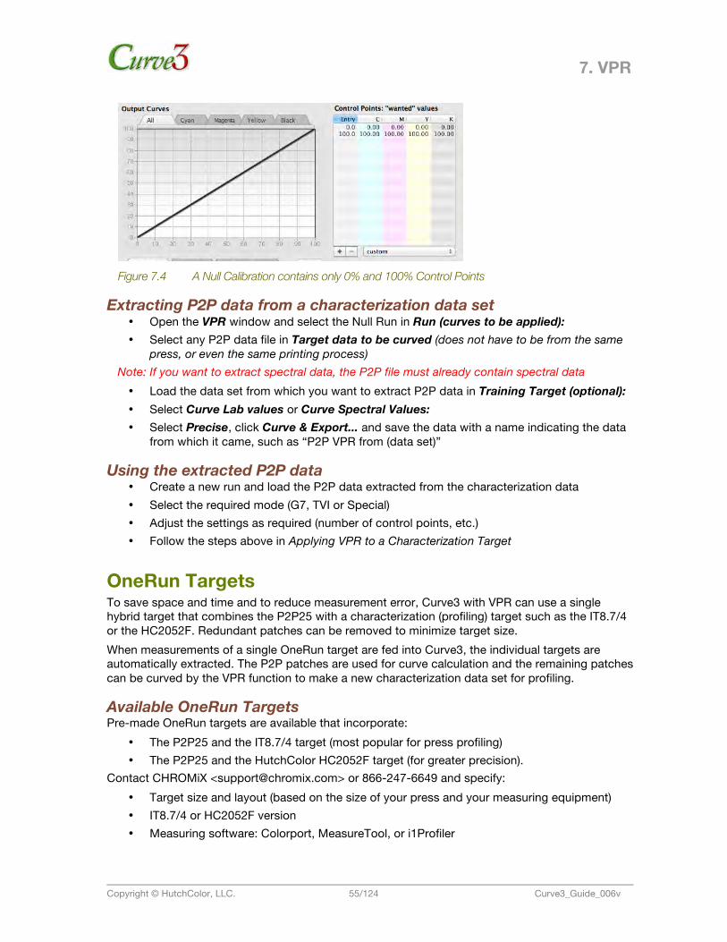
7. VPR
Copyright © HutchColor, LLC. 55/124 Curve3_Guide_006v
Figure 7.4 A Null Calibration contains only 0% and 100% Control Points
Extracting P2P data from a characterization data set • Open the VPR window and select the Null Run in Run (curves to be applied): • Select any P2P data file in Target data to be curved (does not have to be from the same
press, or even the same printing process) Note: If you want to extract spectral data, the P2P file must already contain spectral data • Load the data set from which you want to extract P2P data in Training Target (optional): • Select Curve Lab values or Curve Spectral Values: • Select Precise, click Curve & Export... and save the data with a name indicating the data
from which it came, such as “P2P VPR from (data set)”
Using the extracted P2P data • Create a new run and load the P2P data extracted from the characterization data • Select the required mode (G7, TVI or Special) • Adjust the settings as required (number of control points, etc.) • Follow the steps above in Applying VPR to a Characterization Target
OneRun Targets To save space and time and to reduce measurement error, Curve3 with VPR can use a single hybrid target that combines the P2P25 with a characterization (profiling) target such as the IT8.7/4 or the HC2052F. Redundant patches can be removed to minimize target size. When measurements of a single OneRun target are fed into Curve3, the individual targets are automatically extracted. The P2P patches are used for curve calculation and the remaining patches can be curved by the VPR function to make a new characterization data set for profiling.
Available OneRun Targets Pre-made OneRun targets are available that incorporate:
• The P2P25 and the IT8.7/4 target (most popular for press profiling) • The P2P25 and the HutchColor HC2052F target (for greater precision).
Contact CHROMiX <[email protected]> or 866-247-6649 and specify: • Target size and layout (based on the size of your press and your measuring equipment) • IT8.7/4 or HC2052F version • Measuring software: Colorport, MeasureTool, or i1Profiler
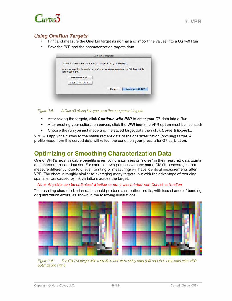
7. VPR
Copyright © HutchColor, LLC. 56/124 Curve3_Guide_006v
Using OneRun Targets • Print and measure the OneRun target as normal and import the values into a Curve3 Run • Save the P2P and the characterization targets data
Figure 7.5 A Curve3 dialog lets you save the component targets
• After saving the targets, click Continue with P2P to enter your G7 data into a Run • After creating your calibration curves, click the VPR icon (the VPR option must be licensed) • Choose the run you just made and the saved target data then click Curve & Export...
VPR will apply the curves to the measurement data of the characterization (profiling) target. A profile made from this curved data will reflect the condition your press after G7 calibration.
Optimizing or Smoothing Characterization Data One of VPR’s most valuable benefits is removing anomalies or “noise” in the measured data points of a characterization data set. For example, two patches with the same CMYK percentages that measure differently (due to uneven printing or measuring) will have identical measurements after VPR. The effect is roughly similar to averaging many targets, but with the advantage of reducing spatial errors caused by ink variations across the target.
Note: Any data can be optimized whether or not it was printed with Curve3 calibration The resulting characterization data should produce a smoother profile, with less chance of banding or quantization errors, as shown in the following illustrations.
Figure 7.6 The IT8.7/4 target with a profile made from noisy data (left) and the same data after VPR-optimization (right)
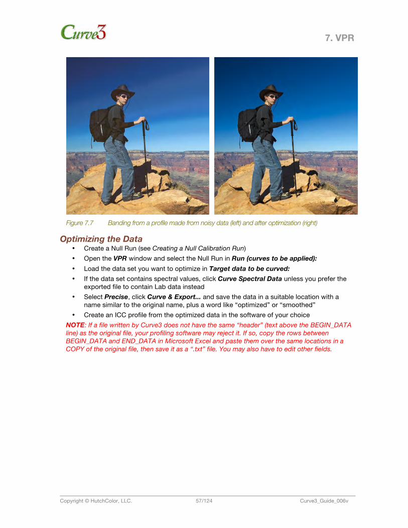
7. VPR
Copyright © HutchColor, LLC. 57/124 Curve3_Guide_006v
Figure 7.7 Banding from a profile made from noisy data (left) and after optimization (right)
Optimizing the Data • Create a Null Run (see Creating a Null Calibration Run) • Open the VPR window and select the Null Run in Run (curves to be applied): • Load the data set you want to optimize in Target data to be curved: • If the data set contains spectral values, click Curve Spectral Data unless you prefer the
exported file to contain Lab data instead • Select Precise, click Curve & Export... and save the data in a suitable location with a
name similar to the original name, plus a word like “optimized” or “smoothed” • Create an ICC profile from the optimized data in the software of your choice
NOTE: If a file written by Curve3 does not have the same “header” (text above the BEGIN_DATA line) as the original file, your profiling software may reject it. If so, copy the rows between BEGIN_DATA and END_DATA in Microsoft Excel and paste them over the same locations in a COPY of the original file, then save it as a “.txt” file. You may also have to edit other fields.
USER GUIDE
Copyright © HutchColor, LLC. 58/124 Curve3_Guide_006v
8. 8. G7 Calibration Workflow This section takes you step-by-step through a typical G7 calibration workflow in Curve3.
Note: These notes assume you are already familiar with Curve3’s controls and functions as described in the previous sections.
Workflow Summary • Print one or more P2P targets • Measure the P2P targets • Load measurement files into Curve3 • Adjust gray balance and other parameters • Select required Control Points • Apply Control Points values to the RIP • Print a new P2P Target through new curves • Verify G7 calibration accuracy
Print the P2P target(s) (See Appendix: A – Target Printing.)
Measure the P2P targets (See Appendix: B – Target Measuring.)
Load measurement files into Curve3 • Click on Run 1 - Calibration in the Runs list. • If the Measurements panel is not visible, click on the Measurements tab to reveal it. • In the Measurements panel either drag and drop P2P measurement file(s) into the
Measurements list, or click on the Plus “+” button below the list and browse for the files.
8. G7 CALIBRATION WORKFLOW
Copyright © HutchColor, LLC. 59/124 Curve3_Guide_006v
Select Based On: Status If this is a new calibration using linear plates or starting curves, leave the Based On: list in the Create Curves window set to Linear (none). If the press run was made through a non-linear RIP curve – e.g. a previous linearization curve, you can select that curve in the Based On: list, (see Section 5. The Based On List).
Adjust gray balance parameters • Click on the Create Curves tab. • Open the Gray Balance Control tab and set the desired threshold, etc.
Choose Control Points In the Control Points list select the required number and values of curve points. Start with a pre-set list and add points as necessary using the Plus + button below the list.
Apply Control Points values to the RIP To type the Control Point correction values into your RIP you can either read them directly from the Create Curves window, or print the list of curve points in a Calibration Run Report. If your RIP accepts digital files directly from Curve3, select the RIP name in the Export... list, then click Export... and import the resulting file into your RIP. For more information see Section 11: Applying Correction Values.
Print a new P2P Target through new curves To confirm the Control Points were effective, print one or more new P2P targets through the new RIP curves. Be sure to use identical ink, substrate and conditions (except for the new RIP curves) as when you printed the first P2P target.
Verify G7 calibration accuracy G7 accuracy can be verified in Curve3 either by creating a new (Verification) Run in the Calibration window or by loading a measured target in the G7 Verify window.
Verifying G7 calibration with a new Run Note that all graphs and results displayed in the new Verification Run are based on an average of all selected samples in the list, not an average of all samples.
• Under the Runs list click the “+” symbol to create a new Run. The default name will be Run (#) – Verification(#) but you can change the name by clicking on it and typing.
• Load one or more P2P measurement file(s) printed through the RIP curves into the Measurements list.
• Click on the Analyze tab. • Click on G7 in the Tests menu. • Check the Curve Shape (delta-L) graph. • Check the Gray Balance (delta-Ch) graph. • Check the delta-L* and delta-Ch values in the Results chart are acceptable

8. G7 CALIBRATION WORKFLOW
Copyright © HutchColor, LLC. 60/124 Curve3_Guide_006v
Using the G7 Verify window Note that all graphs and results displayed in the G7 / TVI Verify window run are based on a single sample highlighted in the list.
• Click the Verify button to open the G7 Verify window. • Load a measurement file from a new target that was printed through the RIP curves. Note
that the target does NOT have to be a P2P, however depending on what target was used some graphs may be invisible or may not display correctly.
• Click the G7 tab. • Check the Curve Shape (delta-L) graph. • Check the Gray Balance (delta-Ch) graph. • Check the delta-L* and delta-Ch values in the Results chart are within acceptable
tolerances – correct numbers have a light green background .
USER GUIDE
Copyright © HutchColor, LLC. 61/124 Curve3_Guide_006v
9. 9. TVI Calibration Workflow This section takes you step-by-step through a typical TVI calibration workflow in Curve3.
Note: These notes assume you are already familiar with Curve3’s controls and functions as described in the previous sections.
Workflow Summary • Print one or more P2P targets • Measure the P2P targets • Change the calibration mode to TVI in the Setup window • Select the desired TVI target curves for each ink • Load measurement files into Curve3 • Select required Control Points • Apply Control Points values to the RIP • Print a new P2P Target through new curves • Verify TVI calibration accuracy
Print the P2P target(s) (See Appendix: A – Target Printing.)
Measure the P2P targets (See Appendix: B – Target Measuring.)
Change Calibration mode to TVI In the Setup window change the Method: to TVI.
9. TVI CALIBRATION WORKFLOW
Copyright © HutchColor, LLC. 62/124 Curve3_Guide_006v
Select TVI Target Curves Select the desired TVI aim curves for each channel. You can choose different aim curves for each channel from the six standard ISO 12647-2 curves, A through F, representing legacy printing from positive and negative film-based plates, or you can load custom TVI curves as follows:
Working with custom TVI Target Curves With custom TVI Target Curves you can imitate the TVI of a previous press run or a custom (non-standard) press condition. To create a custom TVI reference curve set, see Appendix: F. Custom TVI Curves
• Select the custom TVI target curve in the Load Custom TVI list in the Setup window - this replaces all the target curves for C, M, Y and K
• If you want to use one of the standard ISO curves for one or more inks, first load the Custom Target Curve set, then select the desired ISO curve for that individual ink.
Load measurement files into Curve3 • Click on Run 1 - Calibration in the Calibrate runs list. • If the Measurements panel is not visible, click on the Measurements tab to reveal it. • In the Measurements panel either drag and drop P2P measurement file(s) into the
Measurements list, or click on the Plus + button below the list and browse for the files.
Choose Control Points In the Control Points list select the required number and values of curve points.
Leave Gray Balance ON The Gray Balance switch controls whether three separate RIP values are created for C, M and Y or just one. If Gray Balance is ON, the desired TVI curves will be matched with different RIP curve values for each ink. If Gray Balance is OFF, the Cyan RIP curve values will be copied to Magenta and Yellow and one or more of the individual inks may not match their desired TVI curves.
Apply Control Points values to the RIP To type the Control Point correction values into your RIP you can either read them directly from the Create Curves screen, or print the list of curve points in a Calibration Run Report. If your RIP accepts digital files directly from Curve3, select the RIP name in the Export... list, then click Export...and import the resulting file into your RIP. For more information see Section 11: Applying Control Point Values.
Print a new Target through new curves To find out if the Control Points are effective, print one or more new P2P targets through the new RIP curves. Be sure to use identical ink, substrate and conditions (except for the new RIP curves) as when you printed the first target.

9. TVI CALIBRATION WORKFLOW
Copyright © HutchColor, LLC. 63/124 Curve3_Guide_006v
Verify TVI calibration accuracy TVI accuracy can be verified in Curve3 either by creating a new Verification Run in the Calibrate window or by loading a measured target in the Verify window.
Verifying TVI calibration with a new Run Note that all graphs and results displayed in the new Verification run are based on an average of all selected (checked) samples in the list.
• Under the Runs list click the Plus “+” symbol to create a new Calibration Run. The default name will be Run (#) – Verification(#) but you can change the name by clicking on it
• Load one or more P2P measurement file(s) into the Measurements list • Click on the Analyze tab • Click the TVI tab • Check that the CMYK TVI curves match the target TVI curves
USER GUIDE
Copyright © HutchColor, LLC. 64/124 Curve3_Guide_006v
10. 10. Special Ink Calibration Workflow This section takes you step-by-step through a typical Special Ink calibration workflow in Curve3.
Note: These notes assume you are already familiar with Curve3’s controls and functions as described in the previous sections.
Workflow Summary • Print one or more P2P targets using any desired ink colors in place of the normal Cyan,
Magenta, Yellow or Black inks • Measure the P2P targets • In the Setup window change the calibration mode to Special Inks • Load measurement files into Curve3 • Select required Control Points • Apply Control Points values to the RIP • Print a new P2P Target through new curves • Verify calibration accuracy
Print the P2P target(s) (See Appendix: A – Target Printing.)
Measure the P2P targets (See Appendix: B – Target Measuring.)
Change Calibration mode to Special Inks In the Setup window change the Curve Method: to Special Inks.
10. SPECIAL INK CALIBRATION WORKFLOW
Copyright © HutchColor, LLC. 65/124 Curve3_Guide_006v
Load measurement files into Curve3 • Click on Run 1 - Calibration in the Calibrate runs list • If the Measurements panel is not visible, click on the Measurements tab to reveal it • In the Measurements panel either drag and drop P2P measurement file(s) into the
Measurements list, or click on the Plus “+” button below the list and browse for the files
Choose Control Points In the Control Points list select the required number and values of curve points.
Ignore the Gray Balance Switch The Gray Balance switch has no effect in Special Inks mode.
Apply Control Point values to the RIP To type the Control Point correction values into your RIP you can either read them directly from the Create Curves screen, or print the list of curve points in a Calibration Run Report. If your RIP accepts digital files directly from Curve3, select the RIP name in the Export... list, then click Export... and import the resulting file into your RIP. For more information see Section 11: Applying Control Point Values.
Print a new Target through new curves To find out if the Control Points are effective, print one or more new P2P targets through the new RIP curves. Be sure to use identical ink, substrate and printing conditions (except for the new RIP curves) as when you printed the first target.
Verify Special Ink calibration accuracy Special Ink accuracy can be verified in Curve3 by creating a new Verification Run in the Calibrate window.
Verifying Special Ink calibration with a new Run Note that all graphs and results displayed in the new Verification run are based on an average of all selected (checked) samples in the list.
• Under the Runs list click the Plus “+” symbol to create a new Calibration Run. The default name will be Run (#) – Verification(#) but you can change the name by clicking on it.
• Load one or more P2P measurement file(s) into the Measurements list. • Click on the Create Curves tab. • Check that the CMYK Curve Point values are no greater than approximately +/- 1.0%.
USER GUIDE
Copyright © HutchColor, LLC. 66/124 Curve3_Guide_006v
11. 11. Applying Calibration Values The ultimate product of Curve3 is a set of CMYK Control Point values (a.k.a. “calibration curves” or “linearization curves”) that can be applied in several ways:
• In the calibration or linearization section of a CtP (Computer-to-Plate) RIP • In the calibration or linearization section of a film-setter RIP • In the calibration or linearization section of a proofing controller or RIP • In the calibration or linearization section of a digital press controller or RIP • In the calibration or linearization section of an inkjet print controller or RIP • In Adobe Photoshop CS4 (or later) Via DLPs (Device-Link-Profiles) • In Photoshop 6 (or later) via Photoshop Curves
Transferring Curve Values to a RIP Most RIPs and printer drivers provide some form of user-accessible calibration system, but how the calibration system works and what type of information it will accept can vary widely. This section offers general advice on applying the Control Point values produced by Curve3 to the RIP or printer driver. Because calibration utilities differ widely, no single set of instructions will apply to all systems and some experimentation may be necessary. General notes for some specific RIPs are offered in Section 12, RIP-Specific Notes. If your RIP is not mentioned, or you feel the notes are incorrect, please submit comments (ideally with screen images) via the Feedback System…. for inclusion in future updates of this guide. If you are not sure how to apply the Control Point values to your specific RIP or device, see your RIP’s instruction manual or contact your RIP supplier.
Manual entry To type the Control Point values produced by Curve3 into your RIP you can either read them directly from the Create Curves screen, or print the list of curve points in a Calibration Run Report from the File menu or from the Calibration Run Report button.
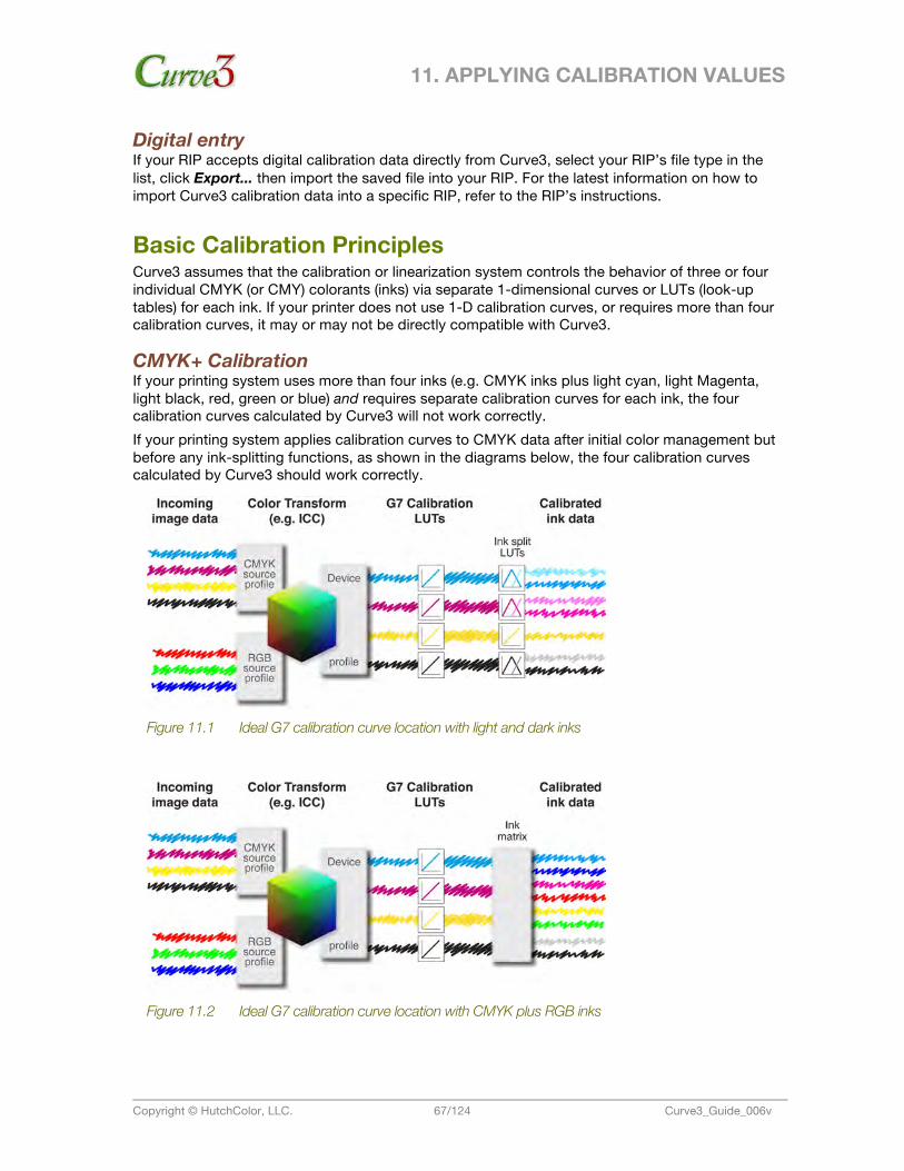
11. APPLYING CALIBRATION VALUES
Copyright © HutchColor, LLC. 67/124 Curve3_Guide_006v
Digital entry If your RIP accepts digital calibration data directly from Curve3, select your RIP’s file type in the list, click Export... then import the saved file into your RIP. For the latest information on how to import Curve3 calibration data into a specific RIP, refer to the RIP’s instructions.
Basic Calibration Principles Curve3 assumes that the calibration or linearization system controls the behavior of three or four individual CMYK (or CMY) colorants (inks) via separate 1-dimensional curves or LUTs (look-up tables) for each ink. If your printer does not use 1-D calibration curves, or requires more than four calibration curves, it may or may not be directly compatible with Curve3.
CMYK+ Calibration If your printing system uses more than four inks (e.g. CMYK inks plus light cyan, light Magenta, light black, red, green or blue) and requires separate calibration curves for each ink, the four calibration curves calculated by Curve3 will not work correctly. If your printing system applies calibration curves to CMYK data after initial color management but before any ink-splitting functions, as shown in the diagrams below, the four calibration curves calculated by Curve3 should work correctly.
Figure 11.1 Ideal G7 calibration curve location with light and dark inks
Figure 11.2 Ideal G7 calibration curve location with CMYK plus RGB inks
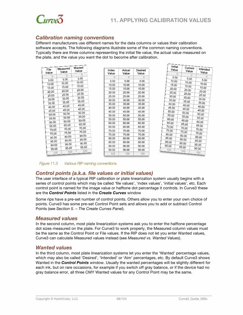
11. APPLYING CALIBRATION VALUES
Copyright © HutchColor, LLC. 68/124 Curve3_Guide_006v
Calibration naming conventions Different manufacturers use different names for the data columns or values their calibration software accepts. The following diagrams illustrate some of the common naming conventions. Typically there are three columns representing the initial file value, the actual value measured on the plate, and the value you want the dot to become after calibration.
Figure 11.3 Various RIP naming conventions.
Control points (a.k.a. file values or initial values) The user interface of a typical RIP calibration or plate linearization system usually begins with a series of control points which may be called ‘file values’, ‘index values’, ‘initial values’, etc. Each control point is named for the image value or halftone dot percentage it controls. In Curve3 these are the Control Points listed in the Create Curves window Some rips have a pre-set number of control points. Others allow you to enter your own choice of points. Curve3 has some pre-set Control Point sets and allows you to add or subtract Control Points (see Section 5. – The Create Curves Panel).
Measured values In the second column, most plate linearization systems ask you to enter the halftone percentage dot sizes measured on the plate. For Curve3 to work properly, the Measured column values must be the same as the Control Point or File values. If the RIP does not let you enter Wanted values, Curve3 can calculate Measured values instead (see Measured vs. Wanted Values).
Wanted values In the third column, most plate linearization systems let you enter the ‘Wanted’ percentage values, which may also be called ‘Desired’, ‘Intended’ or ‘Aim’ percentages, etc. By default Curve3 shows Wanted in the Control Points window. Usually the wanted percentages will be slightly different for each ink, but on rare occasions, for example if you switch off gray balance, or if the device had no gray balance error, all three CMY Wanted values for any Control Point may be the same.
11. APPLYING CALIBRATION VALUES
Copyright © HutchColor, LLC. 69/124 Curve3_Guide_006v
Measured vs. Wanted Values Normally the Control Point values shown in the Create Curves window of Curve3 are the percentage values that each Control Point wants to change to calibration. For example, if the 50% Control Point has a Control Point value of 55%, the device wants to output a 55% value for a Control Point, or incoming file value, of 50%. In other words, 50% tones are darkened by 5%. However a few RIPs demand ‘Measured’ values instead of Wanted values.
If the RIP does not accept Wanted values If your RIP only accepts Measured values (there is no place to enter Wanted values), click the Measured button in the Setup window. The Control Point output values will now be calculated as if they were measured directly from single-color scales on the P2P calibration target, and the RIP should determine the correct Wanted values internally.
Note: The Measured values calculated by Curve3 simulate integrated halftone percentage readings from individual ink scales, but will usually not match percentages measured from the CMY scales of a P2P target, because they include gray balance and NPDC corrections.
G7 Calibration vs. Plate Linearization If your RIP offers two sets of curves for the separate functions of ‘Linearization’ and ‘Tonal editing’, G7 calibration can be performed independently of device linearization by loading the Curve3 calibration values in the Tonal editing curves. However if the RIP has only one set of curves for linearization, with no separate editorial tone correction curves, G7 calibration must use the linearization curves, which normally makes separate plate linearization impractical. In many cases G7 calibration eliminates the need for separate plate linearization, but you still need a way to control plate consistency in production independently of G7 calibration, otherwise a whole new G7 press run would be needed every time the plate system changes. The following section outlines two methods of controlling plate values independently of G7 calibration, on a RIP that has just one set of curves. Both methods work, but one method may be more suitable depending on your specific RIP and workflow needs.
Caution: Small differences in measuring geometry, plate processing, plate emulsion color, etc. can produce different plate dot measurements that may not reflect changes in printed dot size. Re-linearization based on plate measurements can sometimes reduce printing consistency.
Pre-Linearized Method In this method the plates are linearized before G7 calibration and subsequent plate changes are corrected by adding delta values to the G7 Wanted values without needing a new G7 press test.
Warning: This method may result in reduced accuracy.
Initial Linearization • Prior to G7 calibration, linearize the plates as normal using a video plate reader. This will
normally produce different Measured values than Control Point values in the RIP. • Enter the measured values in the linearization section of the RIP, leaving Wanted values
the same as the Control Point values. Caution: Avoid linearizing in finer steps than 10%. Smaller steps may introduce errors caused by the measuring instrument or plate artifacts.
11. APPLYING CALIBRATION VALUES
Copyright © HutchColor, LLC. 70/124 Curve3_Guide_006v
• Expose a new plate and check to see that linearization worked correctly. If it did, the measured plate values should match the Control Point, or File values very closely.
G7 Calibration • Perform a careful G7 calibration press run through the Initial Linearization curves created
above, and measure the P2P target on one or more good printed sheets. • Load the P2P measurement file into Curve3 as normal. • In the Create curves window check the Delta box. • Add the delta values shown to the Wanted values in the RIP. • Expose a new plate and check that the delta values have been achieved on plate, for
example if Curve3 asked for a delta of +3% (increase by 3%) at 50%, where the plate previously measured 50% it should now measure about 53%.
Re-Linearization Re-linearization should not normally be needed unless there has been a significant change in the plate process, for example a new batch of plates or a change in chemistry or laser power.
• To check linearization, temporarily restore the RIP to a linear state, but don’t lose the current Wanted values.
• Expose a new linear plate and measure it. • If the new Measured values are different from the old Measured values (recorded during
the Initial Linearization), enter the new Measured values in the RIP. Note: If the plate system has not changed, the Measured values should be within +/- 1% of what they were originally. • Restore the current Wanted values to restore G7 calibration.
Post-Linearized Method In this method the G7 calibration plates are exposed through a ‘Linear’ or ‘Null’ LUT, but the actual plate values are recorded as ‘Reference Plate Percentages’. Future plate deviations are corrected by editing the G7 Wanted values until a measured plate matches the original Reference Plate Percentages.
Initial Plate Setup • Prior to the G7 calibration run, set the RIP curves so that Control Point, Measured and
Wanted values are identical. This should be the same as loading a ‘Null’ or ‘Linear’ LUT, but see some important cautions later under Specific RIP Notes.
• Produce a set of plates for the G7 calibration run and measure the plate values at 5% or 10% steps.
Note: The actual Measured values do NOT have to be the same as the file values. For example it is not a problem if the 50% dot measures 45%, 53% or similar. • Record these measured values for later reference as Reference Plate Percentages.
G7 Calibration • Perform a careful G7 calibration press run through the same Null curves established in
Initial Plate Setup, and measure the P2P target on one or more good printed sheets. • Load the P2P measurement file into Curve3 as normal.

11. APPLYING CALIBRATION VALUES
Copyright © HutchColor, LLC. 71/124 Curve3_Guide_006v
• In the Create curves window make sure the Delta box is NOT checked. • Enter the Control Point values shown in Curve3 as Wanted values in the RIP. • Make a new plate and check that the wanted changes have been made. For example, if
Curve3 asked for a 50% dot to reduce to 47%, on the plate the 50% patch should measure about 3% less than whatever it measured without the curves, but it does not have to measure 47%.
Note: The actual Measured values do NOT have to be the same as the Wanted values shown in Curve3. It is only necessary that the desired RELATIVE changes have been made compared to the original un-linearized plates. • If the G7-calibrated plates are correct, measure one or more of the plates at 5% or 10%
intervals and record these values as ‘Reference Calibrated Percentages’ for future use when post-linearizing.
Post-Linearization on Top of G7 Calibration This method allows you to make small plate linearization changes due to plate batch differences, and is ideal when only one or two curves are used in the RIP. When many curves are affected simultaneously by a basic optical, chemical or mechanical change in the plate system, Post-Linearization Without G7 Calibration (next item) may be more efficient.
• After any change in the plate process, for example a new batch of plates or a change in processing or laser power, measure a plate made through the active G7 calibration LUTs at 5% or 10% intervals.
• Compare the measured percentages with the Reference Calibrated Percentages recorded in G7 Calibration (above).
• If the measured percentages are different from the Reference Calibrated Percentages, add the DIFFERENCE to the G7 Wanted percentages in the RIP. For example if the 50% file value measured 47% in the Reference Calibrated Percentages, but now reads 45%, add 2% to the current Wanted value at 50%.
• Produce and measure a new plate and check that the measured percentages match the Reference Calibrated Percentages.
Post-Linearization Without G7 Calibration This method is convenient when many G7 curves are affected equally by a basic plate hardware or chemical change that affects all plate workflows. It is also the recommended way to handle plate quality control in general.
• To check the plate process independently of G7 curves, expose a new plate through a Linear or Null LUT.
• Compare the Measured percentages with the Reference Plate Percentages recorded in Initial Plate Setup (above).
• If the Measured percentages are different from the Reference Plate Percentages, adjust laser power or other plate system variables until the measured values match the Reference Plate Percentages.
• Once the measured values match the Reference Plate Percentages, any pre-existing G7 curves should continue to work properly.
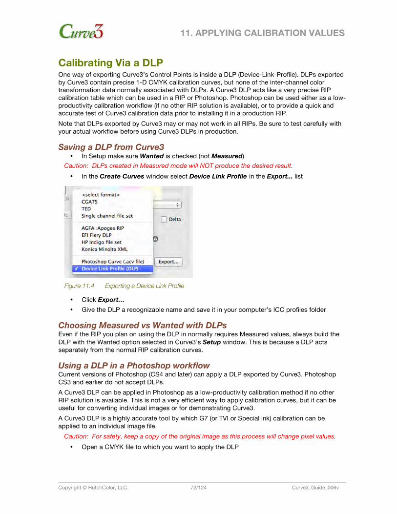
11. APPLYING CALIBRATION VALUES
Copyright © HutchColor, LLC. 72/124 Curve3_Guide_006v
Calibrating Via a DLP One way of exporting Curve3’s Control Points is inside a DLP (Device-Link-Profile). DLPs exported by Curve3 contain precise 1-D CMYK calibration curves, but none of the inter-channel color transformation data normally associated with DLPs. A Curve3 DLP acts like a very precise RIP calibration table which can be used in a RIP or Photoshop. Photoshop can be used either as a low-productivity calibration workflow (if no other RIP solution is available), or to provide a quick and accurate test of Curve3 calibration data prior to installing it in a production RIP. Note that DLPs exported by Curve3 may or may not work in all RIPs. Be sure to test carefully with your actual workflow before using Curve3 DLPs in production.
Saving a DLP from Curve3 • In Setup make sure Wanted is checked (not Measured)
Caution: DLPs created in Measured mode will NOT produce the desired result. • In the Create Curves window select Device Link Profile in the Export... list
Figure 11.4 Exporting a Device Link Profile
• Click Export… • Give the DLP a recognizable name and save it in your computer’s ICC profiles folder
Choosing Measured vs Wanted with DLPs Even if the RIP you plan on using the DLP in normally requires Measured values, always build the DLP with the Wanted option selected in Curve3’s Setup window. This is because a DLP acts separately from the normal RIP calibration curves.
Using a DLP in a Photoshop workflow Current versions of Photoshop (CS4 and later) can apply a DLP exported by Curve3. Photoshop CS3 and earlier do not accept DLPs. A Curve3 DLP can be applied in Photoshop as a low-productivity calibration method if no other RIP solution is available. This is not a very efficient way to apply calibration curves, but it can be useful for converting individual images or for demonstrating Curve3. A Curve3 DLP is a highly accurate tool by which G7 (or TVI or Special ink) calibration can be applied to an individual image file.
Caution: For safety, keep a copy of the original image as this process will change pixel values. • Open a CMYK file to which you want to apply the DLP
11. APPLYING CALIBRATION VALUES
Copyright © HutchColor, LLC. 73/124 Curve3_Guide_006v
• In the Edit menu select Convert to Profile… (If Convert to Profile is not visible, first select Show All Menu Items)
• Click the Advanced button (if visible) • Under Destination Space click the Device Link button • Select the DLP from the Profile: list and click OK
Note: This will immediately apply the calibration curves to your image, but may or may not change its appearance, depending on the strength of the curves • Save the file under a new name to avoid over-writing the original • Send the converted file to the device whose calibration curves made the DLP
Testing RIP accuracy via Photoshop The result of applying a Curve3 DLP in Photoshop should be virtually identical to applying the same control point values in a production printing system or RIP. However in some cases a RIP may produce unexpected results from Curve3 calibration data. This will usually be revealed as a Fail in the Calibrate – Analyze – G7 window (if using the G7 method) or incorrect curves in the Calibrate – Analyze – TVI window. If your RIP accepts calibration curves generated by Curve3, but you suspect the curves have not been applied correctly, follow these steps:
• Print an original1 P2P target with no color management or calibration curves • Perform a G7 calibration and enter Curve3 calibration values in the RIP • Also export a DLP with exactly the same Curve3 settings • Print the same P2P target through the RIP with calibration curves installed but with no
other color management • Measure the printed target and load the data into a new Curve3 Run • Name the Run “RIP method” • Open a CMYK image of the same original P2P target in Photoshop CS4 or later • In the Edit menu select Convert to Profile… (If Convert to Profile is not visible, first select
Show All Menu Items) • Click the Advanced button (if visible) • Under Destination Space click the Device Link button • Select the DLP from the Profile: list and click OK • Save the file under a new name to avoid over-writing the original • Print the converted file with the same settings used to print the original P2P • Measure the printed target and load the data into a new Curve3 Run • Name the Run “Photoshop method” • In the Calibrate window compare the two Runs using the Analyze – Ink & Paper and
Analyze – G7 or (if using the TVI or Special method) Analyze – TVI tab • If the Photoshop method shows a successful calibration but the RIP method does not,
carefully check the way you entered the data into the RIP and if necessary, call your RIP provider for help
1 Be sure the P2P target image is unprocessed and contains the original CMYK percentages
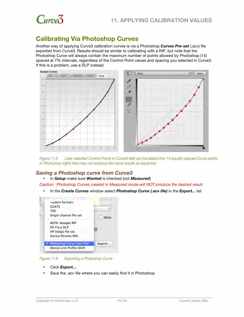
11. APPLYING CALIBRATION VALUES
Copyright © HutchColor, LLC. 74/124 Curve3_Guide_006v
Calibrating Via Photoshop Curves Another way of applying Curve3 calibration curves is via a Photoshop Curves Pre-set (.acv) file exported from Curve3. Results should be similar to calibrating with a RIP, but note that the Photoshop Curve will always contain the maximum number of points allowed by Photoshop (14) spaced at 7% intervals, regardless of the Control Point values and spacing you selected in Curve3. If this is a problem, use a DLP instead.
Figure 11.5 User-selected Control Points in Curve3 (left) are translated into 14 equally-spaced Curve points in Photoshop (right) that may not produce the same results as expected.
Saving a Photoshop curve from Curve3 • In Setup make sure Wanted is checked (not Measured)
Caution: Photoshop Curves created in Measured mode will NOT produce the desired result. • In the Create Curves window select Photoshop Curve (.acv file) in the Export... list
Figure 11.6 Exporting a Photoshop Curve
• Click Export… • Save the .acv file where you can easily find it in Photoshop
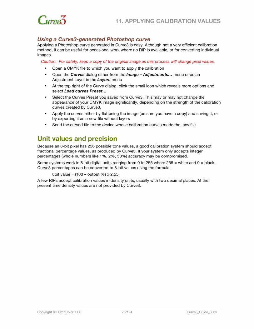
11. APPLYING CALIBRATION VALUES
Copyright © HutchColor, LLC. 75/124 Curve3_Guide_006v
Using a Curve3-generated Photoshop curve Applying a Photoshop curve generated in Curve3 is easy. Although not a very efficient calibration method, it can be useful for occasional work where no RIP is available, or for converting individual images.
Caution: For safety, keep a copy of the original image as this process will change pixel values. • Open a CMYK file to which you want to apply the calibration • Open the Curves dialog either from the Image – Adjustments… menu or as an
Adjustment Layer in the Layers menu • At the top right of the Curve dialog, click the small icon which reveals more options and
select Load curves Preset… • Select the Curves Preset you saved from Curve3. This may or may not change the
appearance of your CMYK image significantly, depending on the strength of the calibration curves created by Curve3.
• Apply the curves either by flattening the image (be sure you have a copy) and saving it, or by exporting it as a new file without layers
• Send the curved file to the device whose calibration curves made the .acv file
Unit values and precision Because an 8-bit pixel has 256 possible tone values, a good calibration system should accept fractional percentage values, as produced by Curve3. If your system only accepts integer percentages (whole numbers like 1%, 2%, 50%) accuracy may be compromised. Some systems work in 8-bit digital units ranging from 0 to 255 where 255 = white and 0 = black. Curve3 percentages can be converted to 8-bit values using the formula:
8bit value = (100 – output %) x 2.55; A few RIPs accept calibration values in density units, usually with two decimal places. At the present time density values are not provided by Curve3.
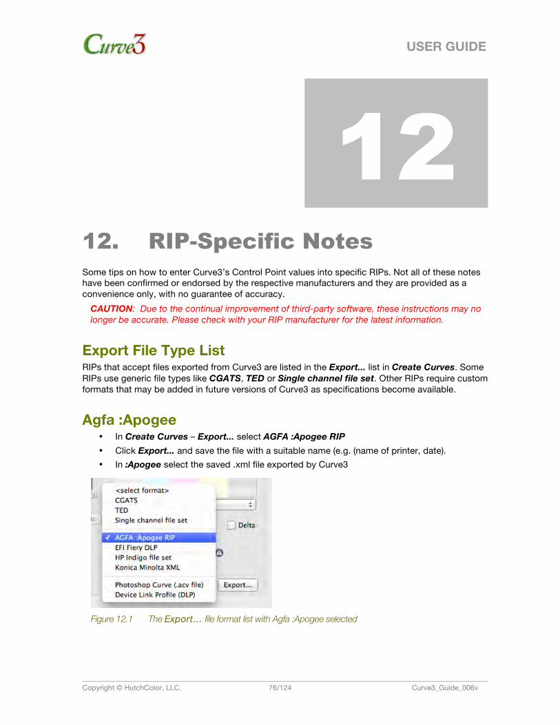
USER GUIDE
Copyright © HutchColor, LLC. 76/124 Curve3_Guide_006v
12. 12. RIP-Specific Notes Some tips on how to enter Curve3’s Control Point values into specific RIPs. Not all of these notes have been confirmed or endorsed by the respective manufacturers and they are provided as a convenience only, with no guarantee of accuracy.
CAUTION: Due to the continual improvement of third-party software, these instructions may no longer be accurate. Please check with your RIP manufacturer for the latest information.
Export File Type List RIPs that accept files exported from Curve3 are listed in the Export... list in Create Curves. Some RIPs use generic file types like CGATS, TED or Single channel file set. Other RIPs require custom formats that may be added in future versions of Curve3 as specifications become available.
Agfa :Apogee • In Create Curves – Export... select AGFA :Apogee RIP • Click Export... and save the file with a suitable name (e.g. (name of printer, date). • In :Apogee select the saved .xml file exported by Curve3
Figure 12.1 The Export... file format list with Agfa :Apogee selected
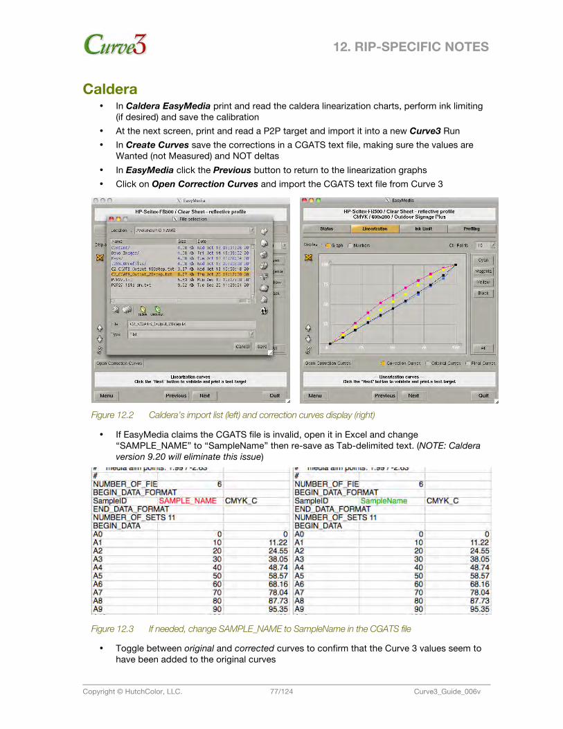
12. RIP-SPECIFIC NOTES
Copyright © HutchColor, LLC. 77/124 Curve3_Guide_006v
Caldera • In Caldera EasyMedia print and read the caldera linearization charts, perform ink limiting
(if desired) and save the calibration • At the next screen, print and read a P2P target and import it into a new Curve3 Run • In Create Curves save the corrections in a CGATS text file, making sure the values are
Wanted (not Measured) and NOT deltas • In EasyMedia click the Previous button to return to the linearization graphs • Click on Open Correction Curves and import the CGATS text file from Curve 3
Figure 12.2 Caldera’s import list (left) and correction curves display (right)
• If EasyMedia claims the CGATS file is invalid, open it in Excel and change “SAMPLE_NAME” to “SampleName” then re-save as Tab-delimited text. (NOTE: Caldera version 9.20 will eliminate this issue)
Figure 12.3 If needed, change SAMPLE_NAME to SampleName in the CGATS file
• Toggle between original and corrected curves to confirm that the Curve 3 values seem to have been added to the original curves
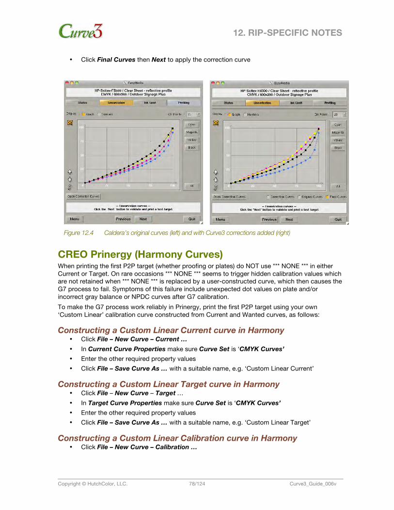
12. RIP-SPECIFIC NOTES
Copyright © HutchColor, LLC. 78/124 Curve3_Guide_006v
• Click Final Curves then Next to apply the correction curve
Figure 12.4 Caldera’s original curves (left) and with Curve3 corrections added (right)
CREO Prinergy (Harmony Curves) When printing the first P2P target (whether proofing or plates) do NOT use *** NONE *** in either Current or Target. On rare occasions *** NONE *** seems to trigger hidden calibration values which are not retained when *** NONE *** is replaced by a user-constructed curve, which then causes the G7 process to fail. Symptoms of this failure include unexpected dot values on plate and/or incorrect gray balance or NPDC curves after G7 calibration. To make the G7 process work reliably in Prinergy, print the first P2P target using your own ‘Custom Linear’ calibration curve constructed from Current and Wanted curves, as follows:
Constructing a Custom Linear Current curve in Harmony • Click File – New Curve – Current … • In Current Curve Properties make sure Curve Set is ‘CMYK Curves’ • Enter the other required property values • Click File – Save Curve As … with a suitable name, e.g. ‘Custom Linear Current’
Constructing a Custom Linear Target curve in Harmony • Click File – New Curve – Target … • In Target Curve Properties make sure Curve Set is ‘CMYK Curves’ • Enter the other required property values • Click File – Save Curve As … with a suitable name, e.g. ‘Custom Linear Target’
Constructing a Custom Linear Calibration curve in Harmony • Click File – New Curve – Calibration …
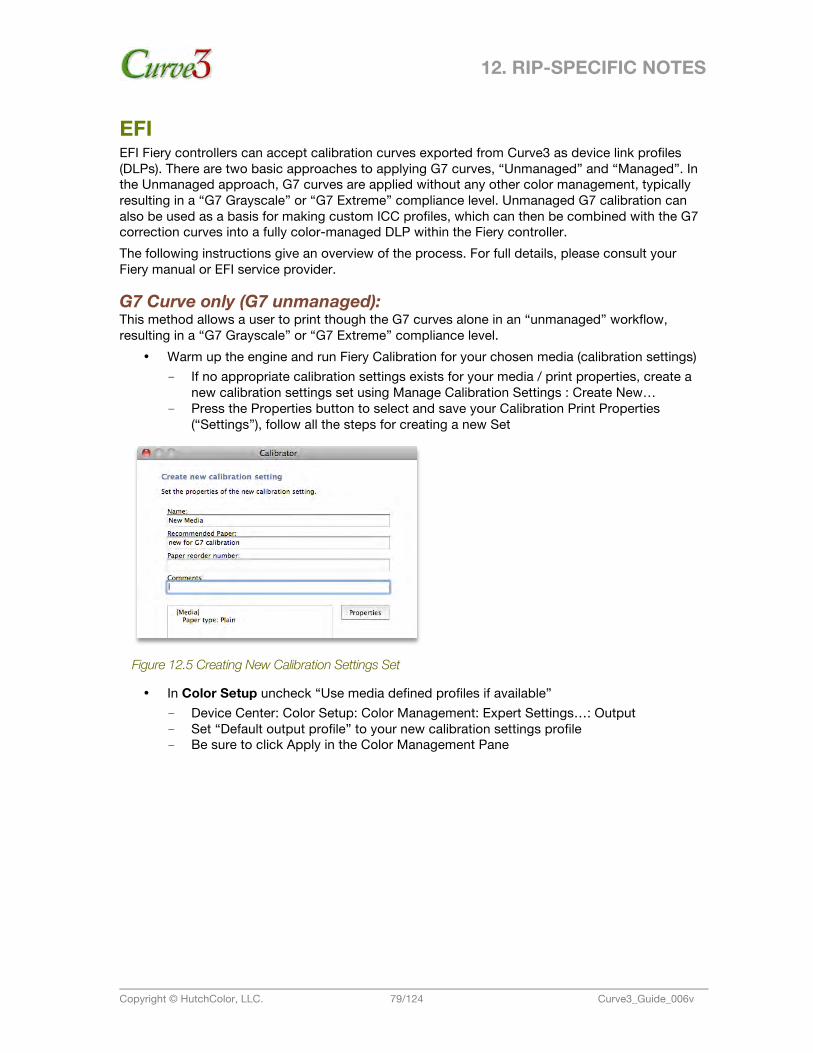
12. RIP-SPECIFIC NOTES
Copyright © HutchColor, LLC. 79/124 Curve3_Guide_006v
EFI EFI Fiery controllers can accept calibration curves exported from Curve3 as device link profiles (DLPs). There are two basic approaches to applying G7 curves, “Unmanaged” and “Managed”. In the Unmanaged approach, G7 curves are applied without any other color management, typically resulting in a “G7 Grayscale” or “G7 Extreme” compliance level. Unmanaged G7 calibration can also be used as a basis for making custom ICC profiles, which can then be combined with the G7 correction curves into a fully color-managed DLP within the Fiery controller. The following instructions give an overview of the process. For full details, please consult your Fiery manual or EFI service provider.
G7 Curve only (G7 unmanaged): This method allows a user to print though the G7 curves alone in an “unmanaged” workflow, resulting in a “G7 Grayscale” or “G7 Extreme” compliance level.
• Warm up the engine and run Fiery Calibration for your chosen media (calibration settings) – If no appropriate calibration settings exists for your media / print properties, create a
new calibration settings set using Manage Calibration Settings : Create New… – Press the Properties button to select and save your Calibration Print Properties
(“Settings”), follow all the steps for creating a new Set
Figure 12.5 Creating New Calibration Settings Set
• In Color Setup uncheck “Use media defined profiles if available” – Device Center: Color Setup: Color Management: Expert Settings…: Output – Set “Default output profile” to your new calibration settings profile – Be sure to click Apply in the Color Management Pane
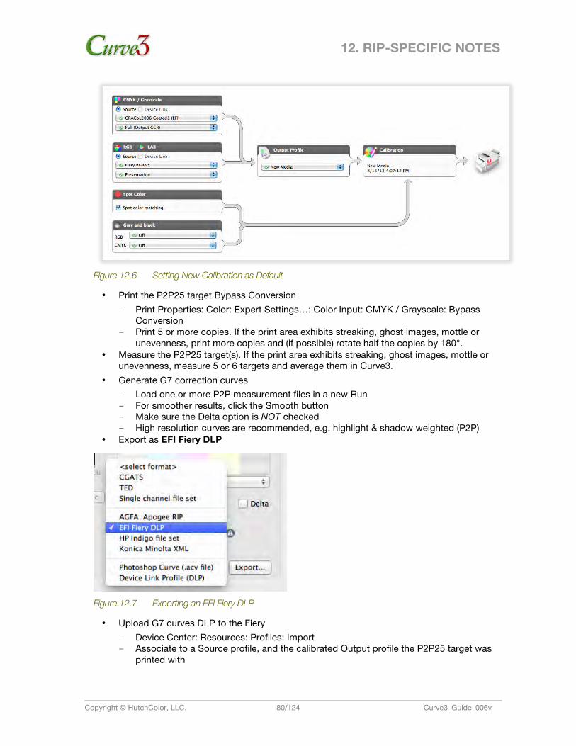
12. RIP-SPECIFIC NOTES
Copyright © HutchColor, LLC. 80/124 Curve3_Guide_006v
Figure 12.6 Setting New Calibration as Default
• Print the P2P25 target Bypass Conversion – Print Properties: Color: Expert Settings…: Color Input: CMYK / Grayscale: Bypass
Conversion – Print 5 or more copies. If the print area exhibits streaking, ghost images, mottle or
unevenness, print more copies and (if possible) rotate half the copies by 180°. • Measure the P2P25 target(s). If the print area exhibits streaking, ghost images, mottle or
unevenness, measure 5 or 6 targets and average them in Curve3. • Generate G7 correction curves
– Load one or more P2P measurement files in a new Run – For smoother results, click the Smooth button – Make sure the Delta option is NOT checked – High resolution curves are recommended, e.g. highlight & shadow weighted (P2P)
• Export as EFI Fiery DLP
Figure 12.7 Exporting an EFI Fiery DLP
• Upload G7 curves DLP to the Fiery – Device Center: Resources: Profiles: Import – Associate to a Source profile, and the calibrated Output profile the P2P25 target was
printed with
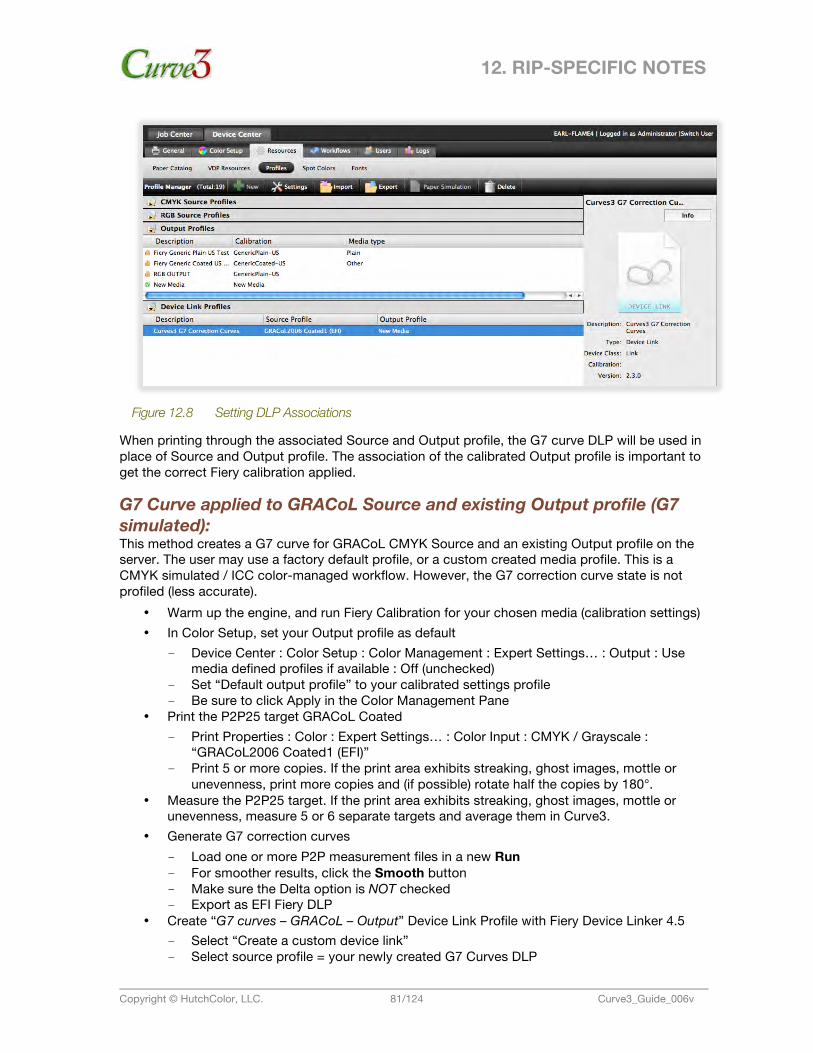
12. RIP-SPECIFIC NOTES
Copyright © HutchColor, LLC. 81/124 Curve3_Guide_006v
Figure 12.8 Setting DLP Associations
When printing through the associated Source and Output profile, the G7 curve DLP will be used in place of Source and Output profile. The association of the calibrated Output profile is important to get the correct Fiery calibration applied.
G7 Curve applied to GRACoL Source and existing Output profile (G7 simulated): This method creates a G7 curve for GRACoL CMYK Source and an existing Output profile on the server. The user may use a factory default profile, or a custom created media profile. This is a CMYK simulated / ICC color-managed workflow. However, the G7 correction curve state is not profiled (less accurate).
• Warm up the engine, and run Fiery Calibration for your chosen media (calibration settings) • In Color Setup, set your Output profile as default
– Device Center : Color Setup : Color Management : Expert Settings… : Output : Use media defined profiles if available : Off (unchecked)
– Set “Default output profile” to your calibrated settings profile – Be sure to click Apply in the Color Management Pane
• Print the P2P25 target GRACoL Coated – Print Properties : Color : Expert Settings… : Color Input : CMYK / Grayscale :
“GRACoL2006 Coated1 (EFI)” – Print 5 or more copies. If the print area exhibits streaking, ghost images, mottle or
unevenness, print more copies and (if possible) rotate half the copies by 180°. • Measure the P2P25 target. If the print area exhibits streaking, ghost images, mottle or
unevenness, measure 5 or 6 separate targets and average them in Curve3. • Generate G7 correction curves
– Load one or more P2P measurement files in a new Run – For smoother results, click the Smooth button – Make sure the Delta option is NOT checked – Export as EFI Fiery DLP
• Create “G7 curves – GRACoL – Output” Device Link Profile with Fiery Device Linker 4.5 – Select “Create a custom device link” – Select source profile = your newly created G7 Curves DLP
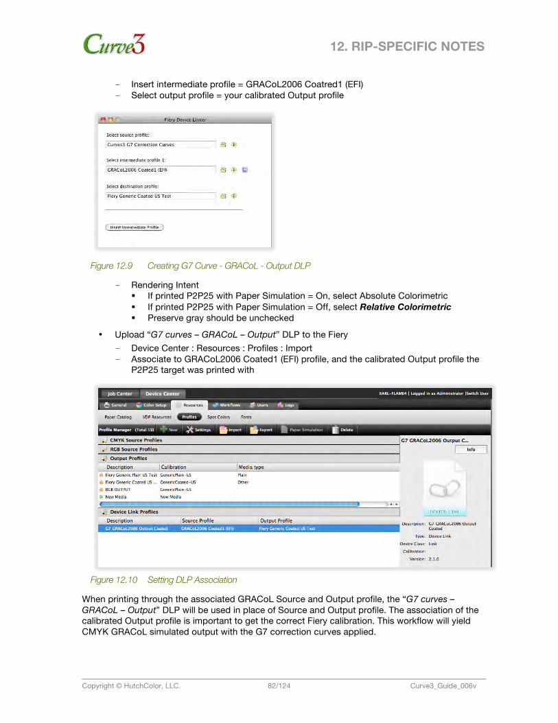
12. RIP-SPECIFIC NOTES
Copyright © HutchColor, LLC. 82/124 Curve3_Guide_006v
– Insert intermediate profile = GRACoL2006 Coatred1 (EFI) – Select output profile = your calibrated Output profile
Figure 12.9 Creating G7 Curve - GRACoL - Output DLP
– Rendering Intent If printed P2P25 with Paper Simulation = On, select Absolute Colorimetric If printed P2P25 with Paper Simulation = Off, select Relative Colorimetric Preserve gray should be unchecked
• Upload “G7 curves – GRACoL – Output” DLP to the Fiery – Device Center : Resources : Profiles : Import – Associate to GRACoL2006 Coated1 (EFI) profile, and the calibrated Output profile the
P2P25 target was printed with
Figure 12.10 Setting DLP Association
When printing through the associated GRACoL Source and Output profile, the “G7 curves – GRACoL – Output” DLP will be used in place of Source and Output profile. The association of the calibrated Output profile is important to get the correct Fiery calibration. This workflow will yield CMYK GRACoL simulated output with the G7 correction curves applied.
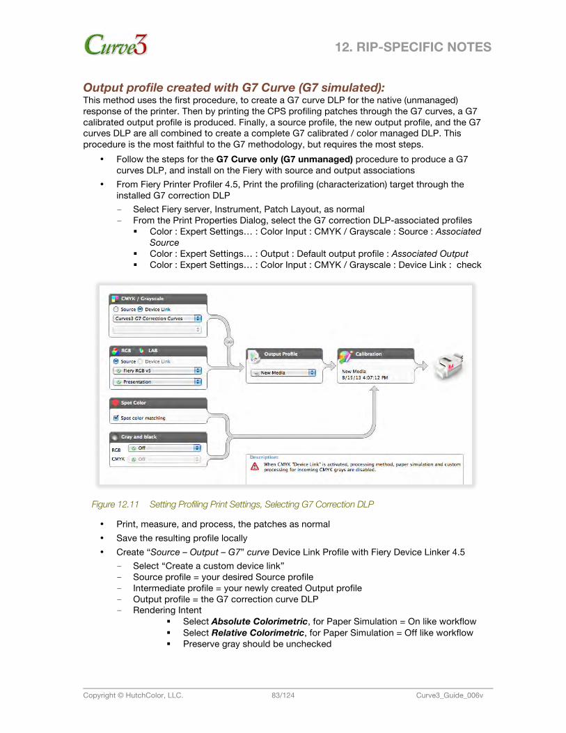
12. RIP-SPECIFIC NOTES
Copyright © HutchColor, LLC. 83/124 Curve3_Guide_006v
Output profile created with G7 Curve (G7 simulated): This method uses the first procedure, to create a G7 curve DLP for the native (unmanaged) response of the printer. Then by printing the CPS profiling patches through the G7 curves, a G7 calibrated output profile is produced. Finally, a source profile, the new output profile, and the G7 curves DLP are all combined to create a complete G7 calibrated / color managed DLP. This procedure is the most faithful to the G7 methodology, but requires the most steps.
• Follow the steps for the G7 Curve only (G7 unmanaged) procedure to produce a G7 curves DLP, and install on the Fiery with source and output associations
• From Fiery Printer Profiler 4.5, Print the profiling (characterization) target through the installed G7 correction DLP – Select Fiery server, Instrument, Patch Layout, as normal – From the Print Properties Dialog, select the G7 correction DLP-associated profiles
Color : Expert Settings… : Color Input : CMYK / Grayscale : Source : Associated Source
Color : Expert Settings… : Output : Default output profile : Associated Output Color : Expert Settings… : Color Input : CMYK / Grayscale : Device Link : check
Figure 12.11 Setting Profiling Print Settings, Selecting G7 Correction DLP
• Print, measure, and process, the patches as normal • Save the resulting profile locally • Create “Source – Output – G7” curve Device Link Profile with Fiery Device Linker 4.5
– Select “Create a custom device link” – Source profile = your desired Source profile – Intermediate profile = your newly created Output profile – Output profile = the G7 correction curve DLP – Rendering Intent
Select Absolute Colorimetric, for Paper Simulation = On like workflow Select Relative Colorimetric, for Paper Simulation = Off like workflow Preserve gray should be unchecked
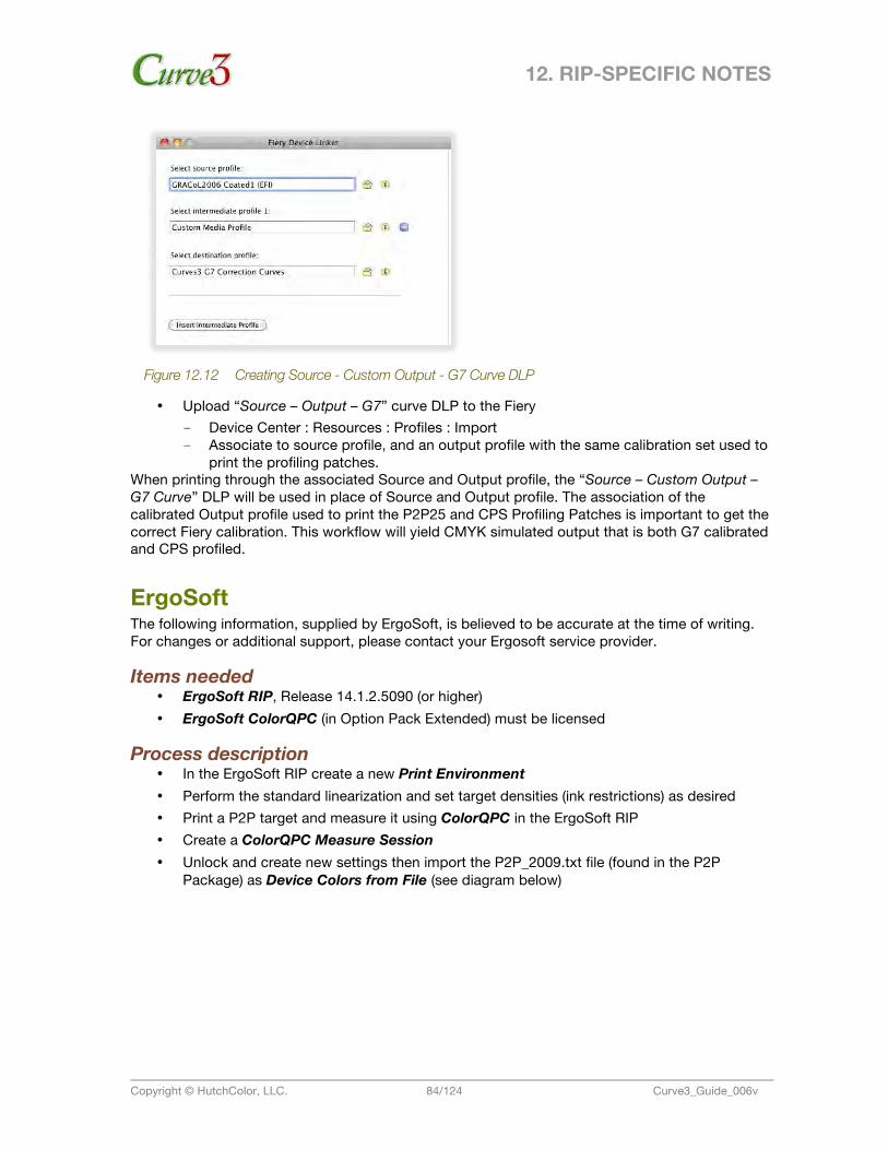
12. RIP-SPECIFIC NOTES
Copyright © HutchColor, LLC. 84/124 Curve3_Guide_006v
Figure 12.12 Creating Source - Custom Output - G7 Curve DLP
• Upload “Source – Output – G7” curve DLP to the Fiery – Device Center : Resources : Profiles : Import – Associate to source profile, and an output profile with the same calibration set used to
print the profiling patches. When printing through the associated Source and Output profile, the “Source – Custom Output – G7 Curve” DLP will be used in place of Source and Output profile. The association of the calibrated Output profile used to print the P2P25 and CPS Profiling Patches is important to get the correct Fiery calibration. This workflow will yield CMYK simulated output that is both G7 calibrated and CPS profiled.
ErgoSoft The following information, supplied by ErgoSoft, is believed to be accurate at the time of writing. For changes or additional support, please contact your Ergosoft service provider.
Items needed • ErgoSoft RIP, Release 14.1.2.5090 (or higher) • ErgoSoft ColorQPC (in Option Pack Extended) must be licensed
Process description • In the ErgoSoft RIP create a new Print Environment • Perform the standard linearization and set target densities (ink restrictions) as desired • Print a P2P target and measure it using ColorQPC in the ErgoSoft RIP • Create a ColorQPC Measure Session • Unlock and create new settings then import the P2P_2009.txt file (found in the P2P
Package) as Device Colors from File (see diagram below)
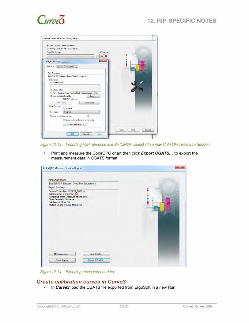
12. RIP-SPECIFIC NOTES
Copyright © HutchColor, LLC. 85/124 Curve3_Guide_006v
Figure 12.13 Importing P2P reference text file (CMYK values) into a new ColorQPC Measure Session
• Print and measure the ColorQPC chart then click Export CGATS… to export the measurement data in CGATS format
Figure 12.14 Exporting measurement data
Create calibration curves in Curve3 • In Curve3 load the CGATS file exported from ErgoSoft in a new Run
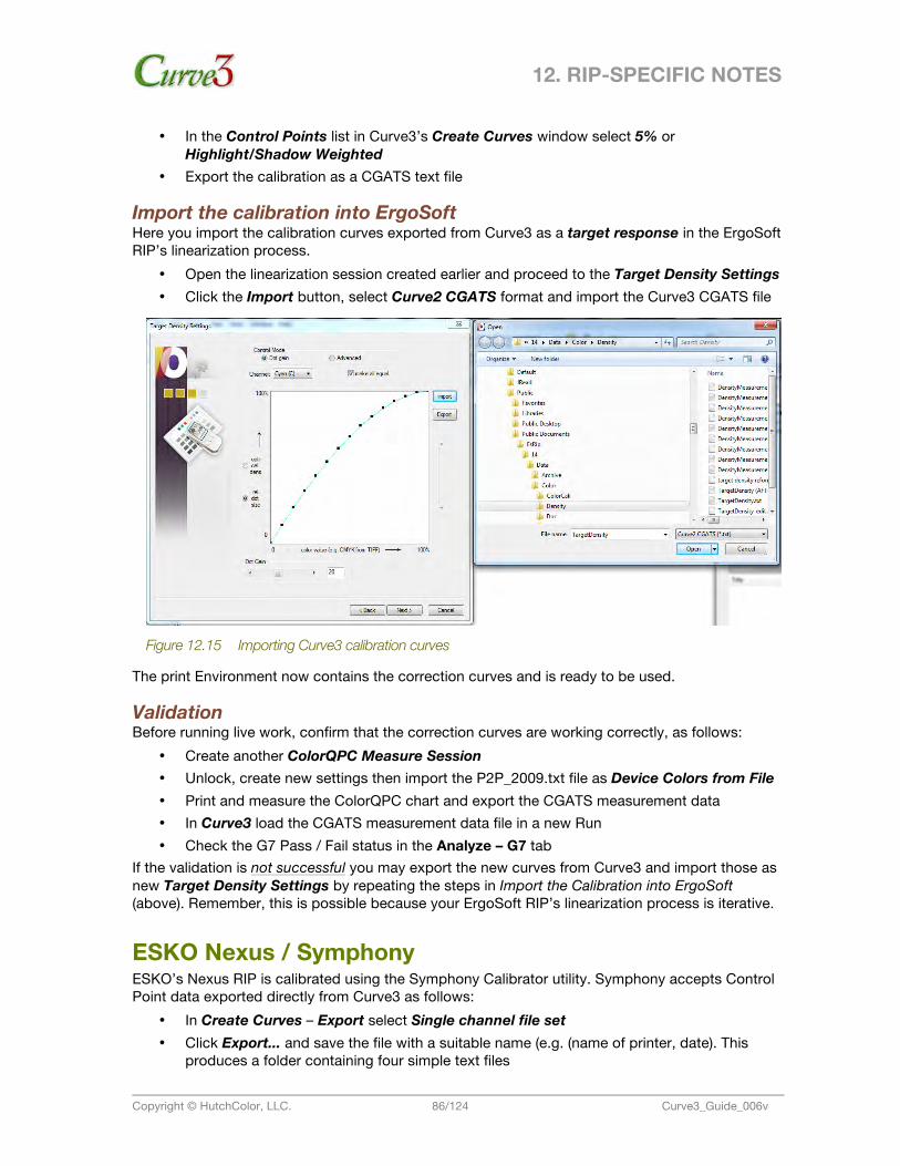
12. RIP-SPECIFIC NOTES
Copyright © HutchColor, LLC. 86/124 Curve3_Guide_006v
• In the Control Points list in Curve3’s Create Curves window select 5% or Highlight/Shadow Weighted
• Export the calibration as a CGATS text file
Import the calibration into ErgoSoft Here you import the calibration curves exported from Curve3 as a target response in the ErgoSoft RIP’s linearization process.
• Open the linearization session created earlier and proceed to the Target Density Settings • Click the Import button, select Curve2 CGATS format and import the Curve3 CGATS file
Figure 12.15 Importing Curve3 calibration curves
The print Environment now contains the correction curves and is ready to be used.
Validation Before running live work, confirm that the correction curves are working correctly, as follows:
• Create another ColorQPC Measure Session • Unlock, create new settings then import the P2P_2009.txt file as Device Colors from File • Print and measure the ColorQPC chart and export the CGATS measurement data • In Curve3 load the CGATS measurement data file in a new Run • Check the G7 Pass / Fail status in the Analyze – G7 tab
If the validation is not successful you may export the new curves from Curve3 and import those as new Target Density Settings by repeating the steps in Import the Calibration into ErgoSoft (above). Remember, this is possible because your ErgoSoft RIP’s linearization process is iterative.
ESKO Nexus / Symphony ESKO’s Nexus RIP is calibrated using the Symphony Calibrator utility. Symphony accepts Control Point data exported directly from Curve3 as follows:
• In Create Curves – Export select Single channel file set • Click Export... and save the file with a suitable name (e.g. (name of printer, date). This
produces a folder containing four simple text files
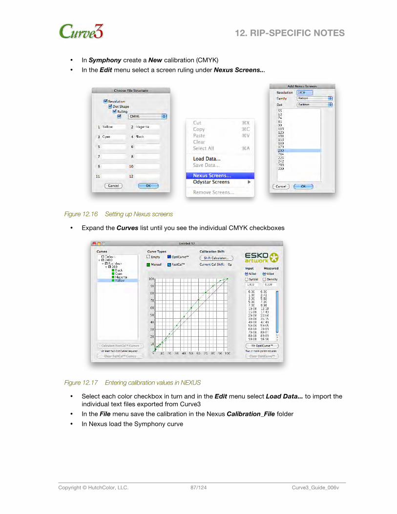
12. RIP-SPECIFIC NOTES
Copyright © HutchColor, LLC. 87/124 Curve3_Guide_006v
• In Symphony create a New calibration (CMYK) • In the Edit menu select a screen ruling under Nexus Screens...
Figure 12.16 Setting up Nexus screens
• Expand the Curves list until you see the individual CMYK checkboxes
Figure 12.17 Entering calibration values in NEXUS
• Select each color checkbox in turn and in the Edit menu select Load Data... to import the individual text files exported from Curve3
• In the File menu save the calibration in the Nexus Calibration_File folder • In Nexus load the Symphony curve
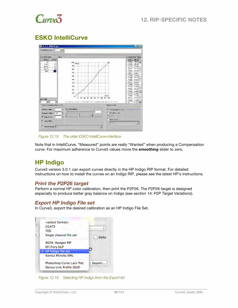
12. RIP-SPECIFIC NOTES
Copyright © HutchColor, LLC. 88/124 Curve3_Guide_006v
ESKO IntelliCurve
Figure 12.18 The older ESKO IntelliCurve interface
Note that in IntelliCurve, “Measured” points are really “Wanted” when producing a Compensation curve. For maximum adherence to Curve3 values move the smoothing slider to zero.
HP Indigo Curve3 version 3.0.1 can export curves directly in the HP Indigo RIP format. For detailed instructions on how to install the curves on an Indigo RIP, please see the latest HP’s instructions.
Print the P2P26 target Perform a normal HP color calibration, then print the P2P26. The P2P26 target is designed especially to produce better gray balance on Indigo (see section 14: P2P Target Variations).
Export HP Indigo File set In Curve3, export the desired calibration as an HP Indigo File Set.
Figure 12.19 Selecting HP Indigo from the Export list
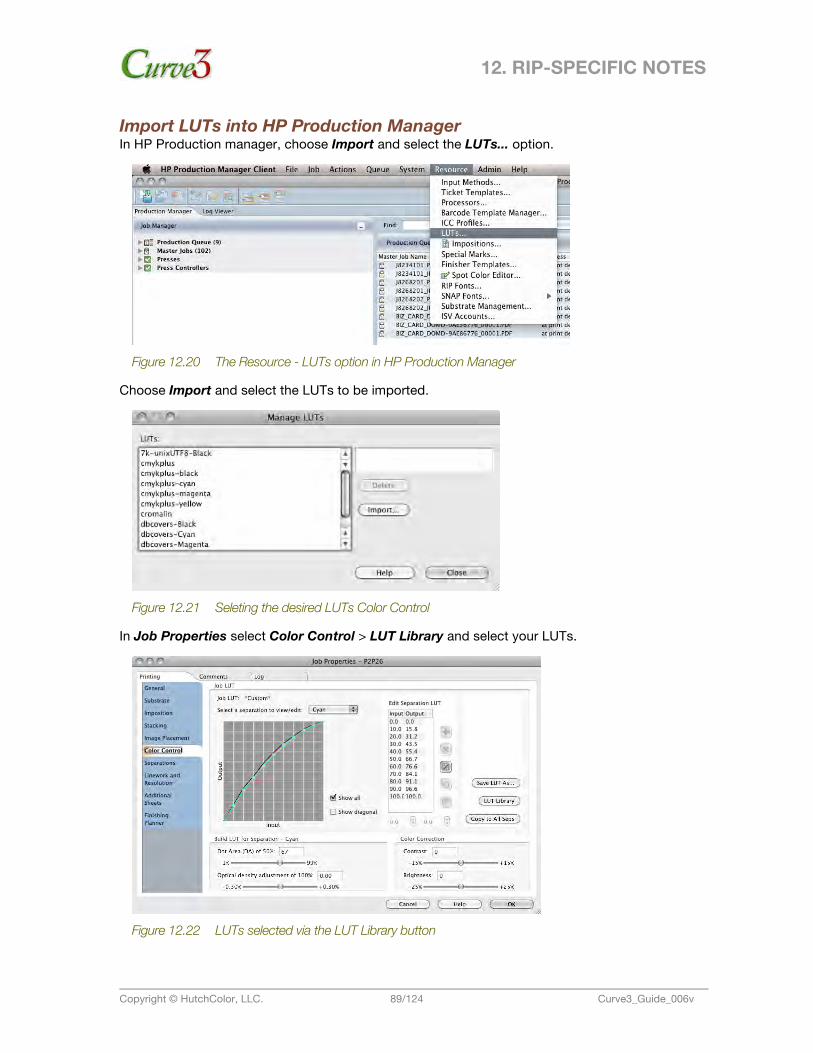
12. RIP-SPECIFIC NOTES
Copyright © HutchColor, LLC. 89/124 Curve3_Guide_006v
Import LUTs into HP Production Manager In HP Production manager, choose Import and select the LUTs... option.
Figure 12.20 The Resource - LUTs option in HP Production Manager
Choose Import and select the LUTs to be imported.
Figure 12.21 Seleting the desired LUTs Color Control
In Job Properties select Color Control > LUT Library and select your LUTs.
Figure 12.22 LUTs selected via the LUT Library button
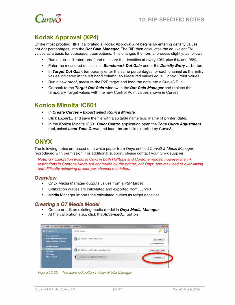
12. RIP-SPECIFIC NOTES
Copyright © HutchColor, LLC. 90/124 Curve3_Guide_006v
Kodak Approval (XP4) Unlike most proofing RIPs, calibrating a Kodak Approval XP4 begins by entering density values, not dot percentages, into the Dot Gain Manager. The RIP then calculates the equivalent TVI values as a basis for subsequent corrections. This changes the normal process slightly, as follows:
• Run an un-calibrated proof and measure the densities at every 10% plus 5% and 95%. • Enter the measured densities in Benchmark Dot Gain under the Density Entry … button. • In Target Dot Gain, temporarily enter the same percentages for each channel as the Entry
values indicated in the left hand column, so Measured values equal Control Point values. • Run a new proof, measure the P2P target and load the data into a Curve3 Run. • Go back to the Target Dot Gain window in the Dot Gain Manager and replace the
temporary Target values with the new Control Point values shown in Curve3.
Konica Minolta IC601 • In Create Curves – Export select Konica Minolta • Click Export... and save the file with a suitable name (e.g. (name of printer, date). • In the Konica Minolta IC601 Color Centro application open the Tone Curve Adjustment
tool, select Load Tone Curve and load the .xml file exported by Curve3.
ONYX The following notes are based on a white paper from Onyx entitled Curve2 & Media Manager, reproduced with permission. For additional support, please contact your Onyx supplier.
Note: G7 Calibration works in Onyx in both Halftone and Contone modes, however the ink restrictions in Contone Mode are controlled by the printer, not Onyx, and may lead to over-inking and difficulty achieving proper per-channel restriction.
Overview • Onyx Media Manager outputs values from a P2P target • Calibration curves are calculated and exported from Curve3 • Media Manager imports the calculated curves as target densities
Creating a G7 Media Model • Create or edit an existing media model in Onyx Media Manager • At the calibration step, click the Advanced… button
Figure 12.20 The advaned button in Onyx Media Manager
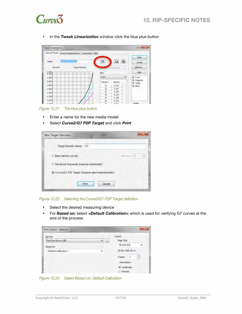
12. RIP-SPECIFIC NOTES
Copyright © HutchColor, LLC. 91/124 Curve3_Guide_006v
• In the Tweak Linearization window click the blue plus button
Figure 12.21 The blue plus button
• Enter a name for the new media model • Select Curve2/G7 P2P Target and click Print
Figure 12.22 Selecting the Curve2/G7 P2P Target definition
• Select the desired measuring device • For Based on: select <Default Calibration> which is used for verifying G7 curves at the
end of the process
Figure 12.23 Select Based on: Default Calibration
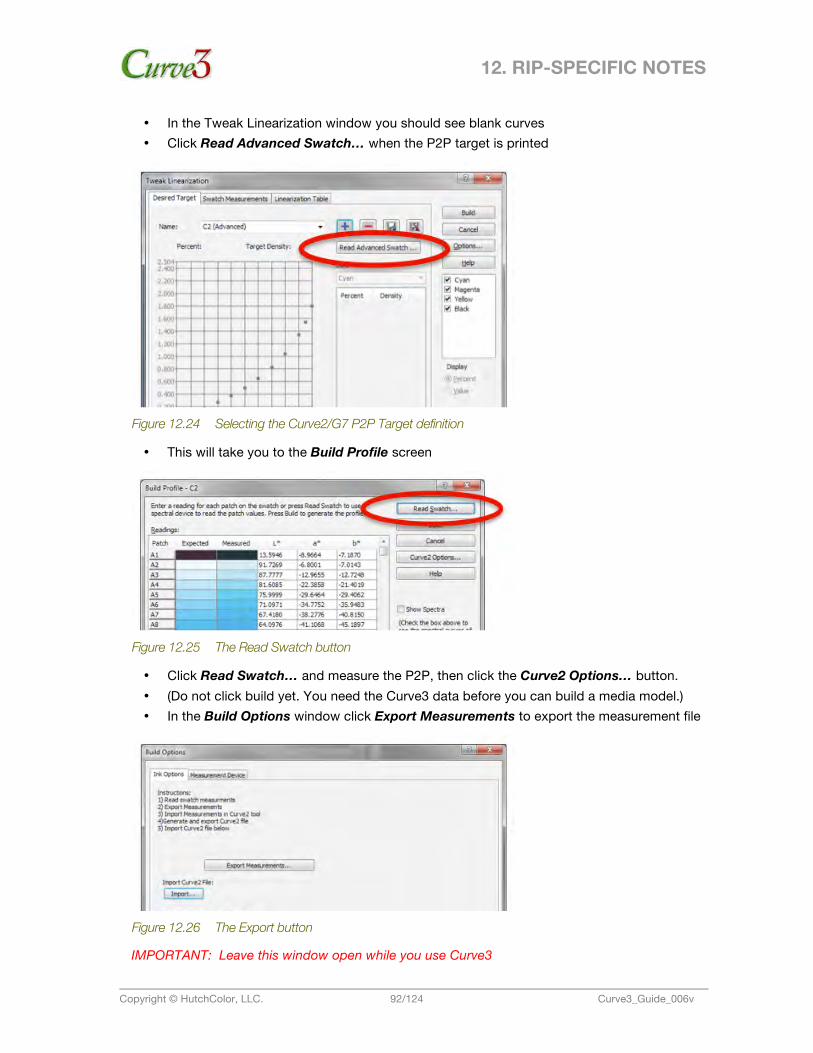
12. RIP-SPECIFIC NOTES
Copyright © HutchColor, LLC. 92/124 Curve3_Guide_006v
• In the Tweak Linearization window you should see blank curves • Click Read Advanced Swatch… when the P2P target is printed
Figure 12.24 Selecting the Curve2/G7 P2P Target definition
• This will take you to the Build Profile screen
Figure 12.25 The Read Swatch button
• Click Read Swatch… and measure the P2P, then click the Curve2 Options… button. • (Do not click build yet. You need the Curve3 data before you can build a media model.) • In the Build Options window click Export Measurements to export the measurement file
Figure 12.26 The Export button
IMPORTANT: Leave this window open while you use Curve3
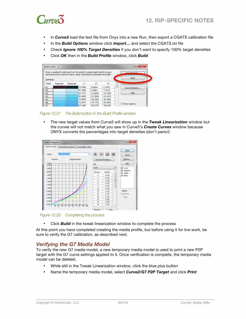
12. RIP-SPECIFIC NOTES
Copyright © HutchColor, LLC. 93/124 Curve3_Guide_006v
• In Curve3 load the text file from Onyx into a new Run, then export a CGATS calibration file • In the Build Options window click Import… and select the CGATS.txt file • Check Ignore 100% Target Densities if you don’t want to specify 100% target densities • Click OK then in the Build Profile window, click Build
Figure 12.27 The Build button in the Build Profile window
• The new target values from Curve3 will show up in the Tweak Linearization window but the curves will not match what you saw in Curve3’s Create Curves window because ONYX converts the percentages into target densities (don’t panic!)
Figure 12.28 Completing the process
• Click Build in the tweak linearization window to complete the process At this point you have completed creating the media profile, but before using it for live work, be sure to verify the G7 calibration, as described next.
Verifying the G7 Media Model To verify the new G7 media model, a new temporary media model is used to print a new P2P target with the G7 curve settings applied to it. Once verification is complete, the temporary media model can be deleted.
• While still in the Tweak Linearization window, click the blue plus button • Name the temporary media model, select Curve2/G7 P2P Target and click Print
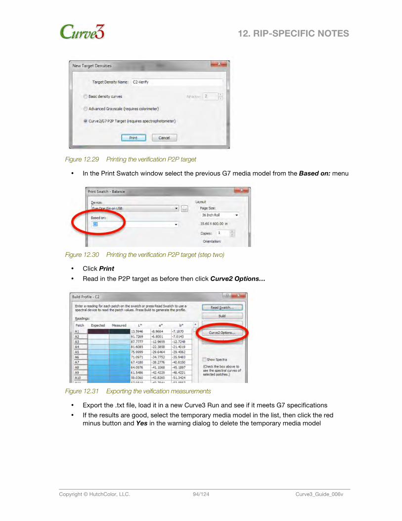
12. RIP-SPECIFIC NOTES
Copyright © HutchColor, LLC. 94/124 Curve3_Guide_006v
Figure 12.29 Printing the verification P2P target
• In the Print Swatch window select the previous G7 media model from the Based on: menu
Figure 12.30 Printing the verification P2P target (step two)
• Click Print • Read in the P2P target as before then click Curve2 Options…
Figure 12.31 Exporting the veification measurements
• Export the .txt file, load it in a new Curve3 Run and see if it meets G7 specifications • If the results are good, select the temporary media model in the list, then click the red
minus button and Yes in the warning dialog to delete the temporary media model
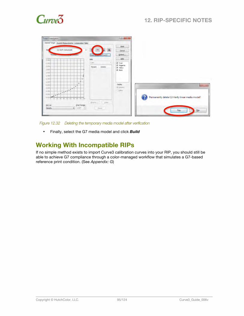
12. RIP-SPECIFIC NOTES
Copyright © HutchColor, LLC. 95/124 Curve3_Guide_006v
Figure 12.32 Deleting the temporary media model after verification
• Finally, select the G7 media model and click Build
Working With Incompatible RIPs If no simple method exists to import Curve3 calibration curves into your RIP, you should still be able to achieve G7 compliance through a color-managed workflow that simulates a G7-based reference print condition. (See Appendix: G)
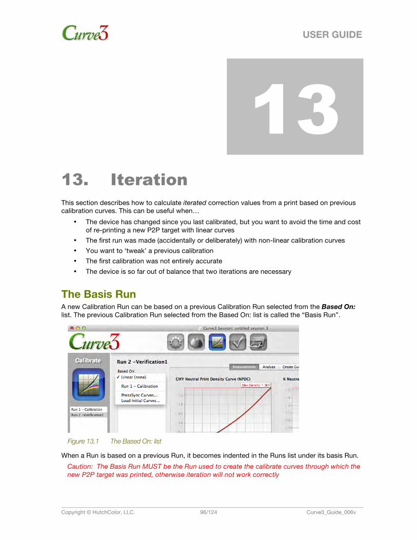
USER GUIDE
Copyright © HutchColor, LLC. 96/124 Curve3_Guide_006v
13. 13. Iteration This section describes how to calculate iterated correction values from a print based on previous calibration curves. This can be useful when…
• The device has changed since you last calibrated, but you want to avoid the time and cost of re-printing a new P2P target with linear curves
• The first run was made (accidentally or deliberately) with non-linear calibration curves • You want to ‘tweak’ a previous calibration • The first calibration was not entirely accurate • The device is so far out of balance that two iterations are necessary
The Basis Run A new Calibration Run can be based on a previous Calibration Run selected from the Based On: list. The previous Calibration Run selected from the Based On: list is called the “Basis Run”.
Figure 13.1 The Based On: list
When a Run is based on a previous Run, it becomes indented in the Runs list under its basis Run. Caution: The Basis Run MUST be the Run used to create the calibrate curves through which the new P2P target was printed, otherwise iteration will not work correctly
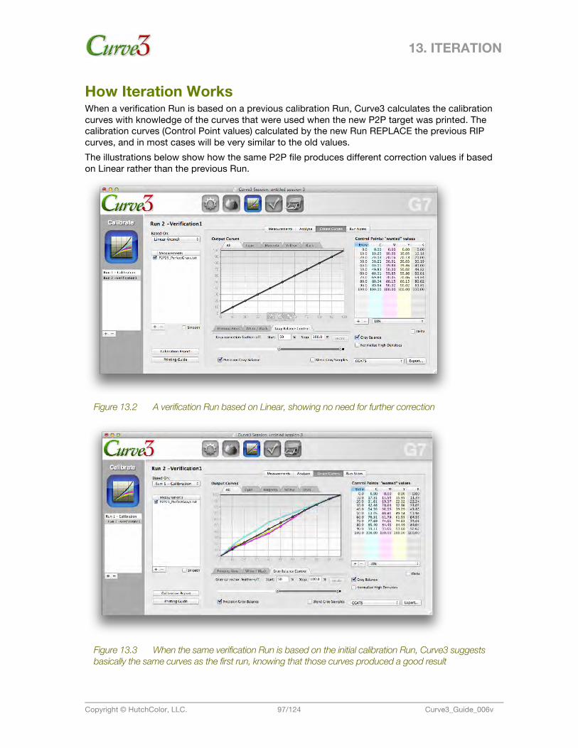
13. ITERATION
Copyright © HutchColor, LLC. 97/124 Curve3_Guide_006v
How Iteration Works When a verification Run is based on a previous calibration Run, Curve3 calculates the calibration curves with knowledge of the curves that were used when the new P2P target was printed. The calibration curves (Control Point values) calculated by the new Run REPLACE the previous RIP curves, and in most cases will be very similar to the old values. The illustrations below show how the same P2P file produces different correction values if based on Linear rather than the previous Run.
Figure 13.2 A verification Run based on Linear, showing no need for further correction
Figure 13.3 When the same verification Run is based on the initial calibration Run, Curve3 suggests basically the same curves as the first run, knowing that those curves produced a good result
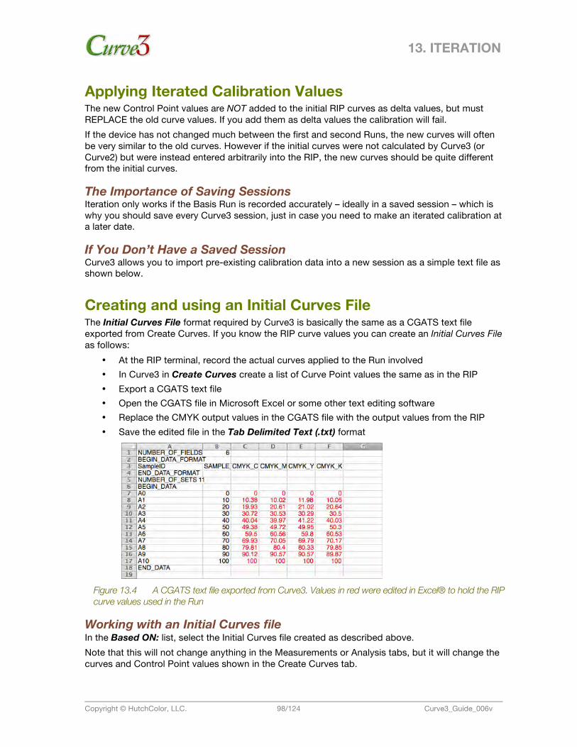
13. ITERATION
Copyright © HutchColor, LLC. 98/124 Curve3_Guide_006v
Applying Iterated Calibration Values The new Control Point values are NOT added to the initial RIP curves as delta values, but must REPLACE the old curve values. If you add them as delta values the calibration will fail. If the device has not changed much between the first and second Runs, the new curves will often be very similar to the old curves. However if the initial curves were not calculated by Curve3 (or Curve2) but were instead entered arbitrarily into the RIP, the new curves should be quite different from the initial curves.
The Importance of Saving Sessions Iteration only works if the Basis Run is recorded accurately – ideally in a saved session – which is why you should save every Curve3 session, just in case you need to make an iterated calibration at a later date.
If You Don’t Have a Saved Session Curve3 allows you to import pre-existing calibration data into a new session as a simple text file as shown below.
Creating and using an Initial Curves File The Initial Curves File format required by Curve3 is basically the same as a CGATS text file exported from Create Curves. If you know the RIP curve values you can create an Initial Curves File as follows:
• At the RIP terminal, record the actual curves applied to the Run involved • In Curve3 in Create Curves create a list of Curve Point values the same as in the RIP • Export a CGATS text file • Open the CGATS file in Microsoft Excel or some other text editing software • Replace the CMYK output values in the CGATS file with the output values from the RIP • Save the edited file in the Tab Delimited Text (.txt) format
Figure 13.4 A CGATS text file exported from Curve3. Values in red were edited in Excel® to hold the RIP curve values used in the Run
Working with an Initial Curves file In the Based ON: list, select the Initial Curves file created as described above. Note that this will not change anything in the Measurements or Analysis tabs, but it will change the curves and Control Point values shown in the Create Curves tab.
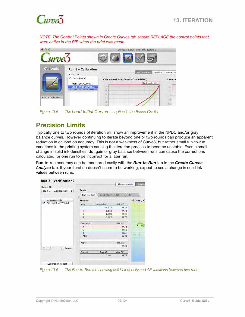
13. ITERATION
Copyright © HutchColor, LLC. 99/124 Curve3_Guide_006v
NOTE: The Control Points shown in Create Curves tab should REPLACE the control points that were active in the RIP when the print was made.
Figure 13.5 The Load Initial Curves ... option in the Based On: list
Precision Limits Typically one to two rounds of iteration will show an improvement in the NPDC and/or gray balance curves. However continuing to iterate beyond one or two rounds can produce an apparent reduction in calibration accuracy. This is not a weakness of Curve3, but rather small run-to-run variations in the printing system causing the iteration process to become unstable. Even a small change in solid ink densities, dot gain or gray balance between runs can cause the corrections calculated for one run to be incorrect for a later run. Run-to-run accuracy can be monitored easily with the Run-to-Run tab in the Create Curves – Analyze tab. If your iteration doesn’t seem to be working, expect to see a change in solid ink values between runs.
Figure 13.6 The Run-to-Run tab showing solid ink density and ∆E variations between two runs

13. ITERATION
Copyright © HutchColor, LLC. 100/124 Curve3_Guide_006v
Avoiding Errors Basing a Calibration Run on a Basis Run can easily go wrong if you are not careful. You must be absolutely sure which Basis Run was used to calibrate prior to the current Run, and the settings in that Basis Run must not have changed, especially the following:
• Measurement files active or disabled in the Measurements list • Number and values of the Control Points • White / Black tab settings • Gray balance On/Off • Gray Balance Control tab settings • Normalize High Densities status • The Basis Run selected in the Based On: list (if any)
Note: A Calibration Run may be based on a Basis Run which was itself based on an earlier Basis Run, which in turn may be based on an even earlier Basis Run, and so on. For Iteration to work correctly it is important that all Basis Runs leading up to the current Run are included in the session, and all Curve3 settings active when each Basis Run was applied have not been altered.
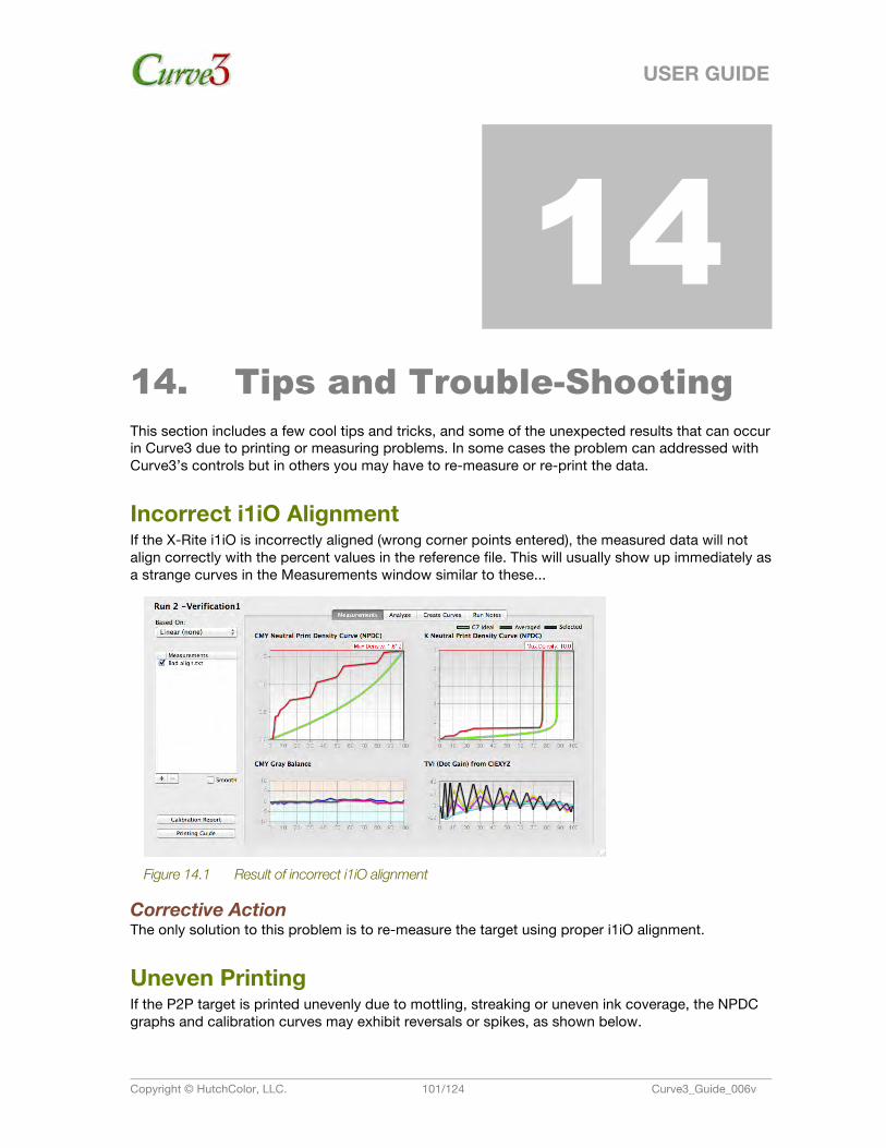
USER GUIDE
Copyright © HutchColor, LLC. 101/124 Curve3_Guide_006v
14. 14. Tips and Trouble-Shooting This section includes a few cool tips and tricks, and some of the unexpected results that can occur in Curve3 due to printing or measuring problems. In some cases the problem can addressed with Curve3’s controls but in others you may have to re-measure or re-print the data.
Incorrect i1iO Alignment If the X-Rite i1iO is incorrectly aligned (wrong corner points entered), the measured data will not align correctly with the percent values in the reference file. This will usually show up immediately as a strange curves in the Measurements window similar to these...
Figure 14.1 Result of incorrect i1iO alignment
Corrective Action The only solution to this problem is to re-measure the target using proper i1iO alignment.
Uneven Printing If the P2P target is printed unevenly due to mottling, streaking or uneven ink coverage, the NPDC graphs and calibration curves may exhibit reversals or spikes, as shown below.
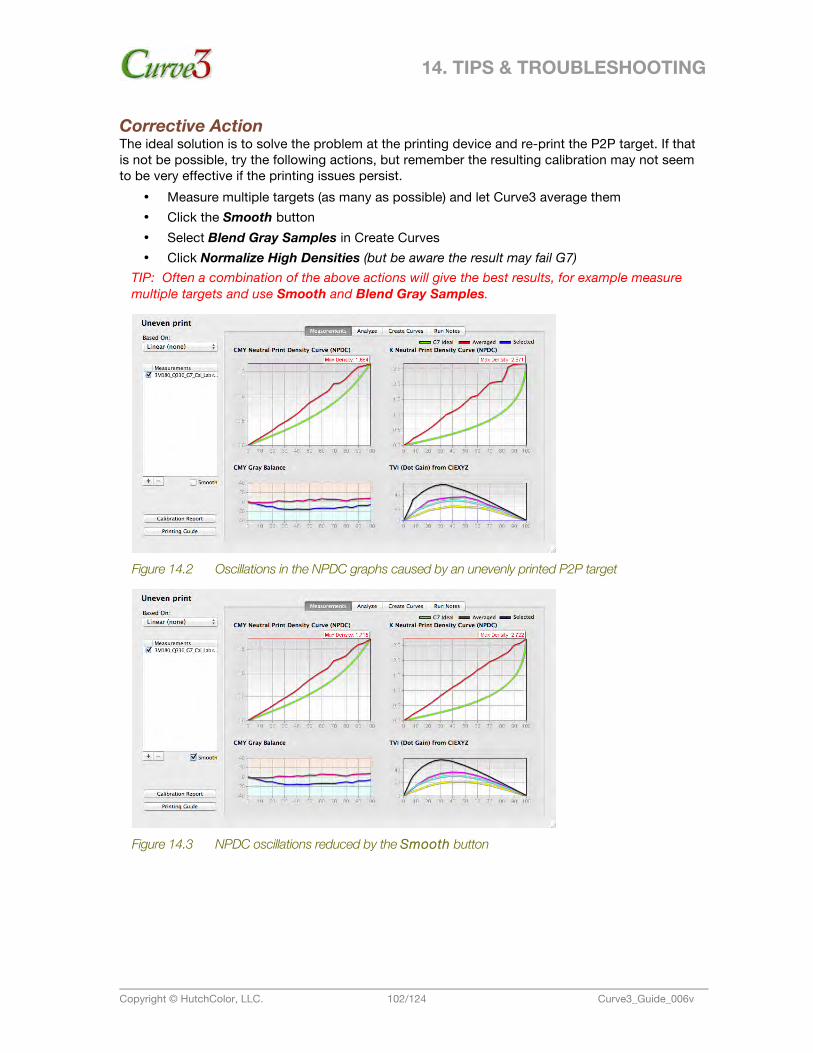
14. TIPS & TROUBLESHOOTING
Copyright © HutchColor, LLC. 102/124 Curve3_Guide_006v
Corrective Action The ideal solution is to solve the problem at the printing device and re-print the P2P target. If that is not be possible, try the following actions, but remember the resulting calibration may not seem to be very effective if the printing issues persist.
• Measure multiple targets (as many as possible) and let Curve3 average them • Click the Smooth button • Select Blend Gray Samples in Create Curves • Click Normalize High Densities (but be aware the result may fail G7)
TIP: Often a combination of the above actions will give the best results, for example measure multiple targets and use Smooth and Blend Gray Samples.
Figure 14.2 Oscillations in the NPDC graphs caused by an unevenly printed P2P target
Figure 14.3 NPDC oscillations reduced by the Smooth button
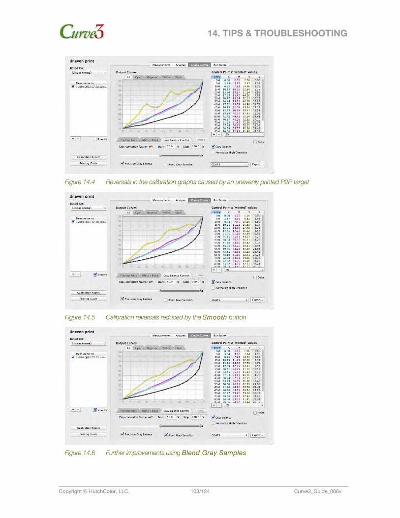
14. TIPS & TROUBLESHOOTING
Copyright © HutchColor, LLC. 103/124 Curve3_Guide_006v
Figure 14.4 Reversals in the calibration graphs caused by an unevenly printed P2P target
Figure 14.5 Calibration reversals reduced by the Smooth button
Figure 14.6 Further improvements using Blend Gray Samples
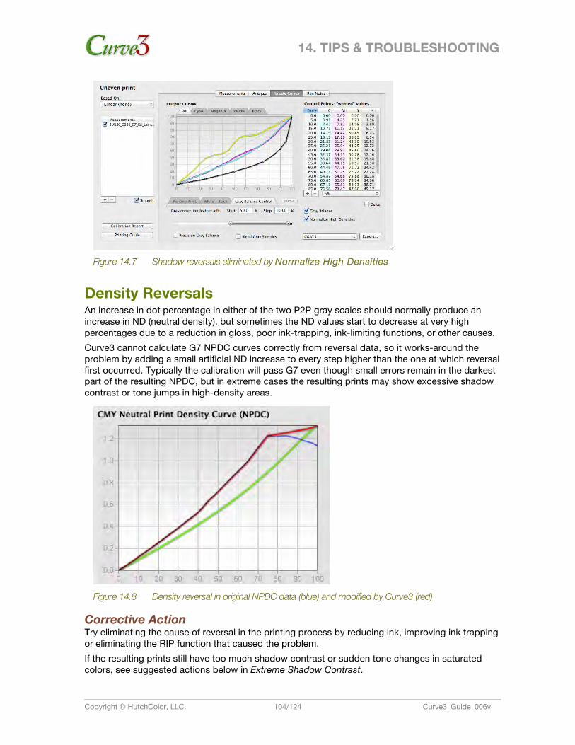
14. TIPS & TROUBLESHOOTING
Copyright © HutchColor, LLC. 104/124 Curve3_Guide_006v
Figure 14.7 Shadow reversals eliminated by Normalize High Densities
Density Reversals An increase in dot percentage in either of the two P2P gray scales should normally produce an increase in ND (neutral density), but sometimes the ND values start to decrease at very high percentages due to a reduction in gloss, poor ink-trapping, ink-limiting functions, or other causes. Curve3 cannot calculate G7 NPDC curves correctly from reversal data, so it works-around the problem by adding a small artificial ND increase to every step higher than the one at which reversal first occurred. Typically the calibration will pass G7 even though small errors remain in the darkest part of the resulting NPDC, but in extreme cases the resulting prints may show excessive shadow contrast or tone jumps in high-density areas.
Figure 14.8 Density reversal in original NPDC data (blue) and modified by Curve3 (red)
Corrective Action Try eliminating the cause of reversal in the printing process by reducing ink, improving ink trapping or eliminating the RIP function that caused the problem. If the resulting prints still have too much shadow contrast or sudden tone changes in saturated colors, see suggested actions below in Extreme Shadow Contrast.
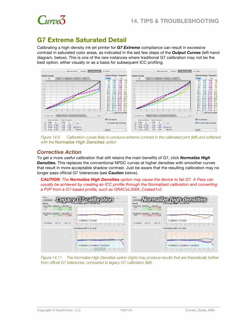
14. TIPS & TROUBLESHOOTING
Copyright © HutchColor, LLC. 105/124 Curve3_Guide_006v
G7 Extreme Saturated Detail Calibrating a high-density ink-jet printer for G7 Extreme compliance can result in excessive contrast in saturated color areas, as indicated in the last few steps of the Output Curves (left-hand diagram, below). This is one of the rare instances where traditional G7 calibration may not be the best option, either visually or as a basis for subsequent ICC profiling.
Figure 14.9 Calibration curves likely to produce extreme contrast in the calibrated print (left) and softened with the Normalize High Densities option
Corrective Action To get a more useful calibration that still retains the main benefits of G7, click Normalize High Densities. This replaces the conventional NPDC curves at higher densities with smoother curves that result in more acceptable shadow contrast. Just be aware that the resulting calibration may no longer pass official G7 tolerances (see Caution below).
CAUTION: The Normalize High Densities option may cause the device to fail G7. A Pass can usually be achieved by creating an ICC profile through the Normalized calibration and converting a P2P from a G7-based profile, such as GRACoL2006_Coated1v2.
Figure 14.11 The Normalize High Densities option (right) may produce results that are theoretically further from official G7 tolerances, compared to legacy G7 calibration (left).
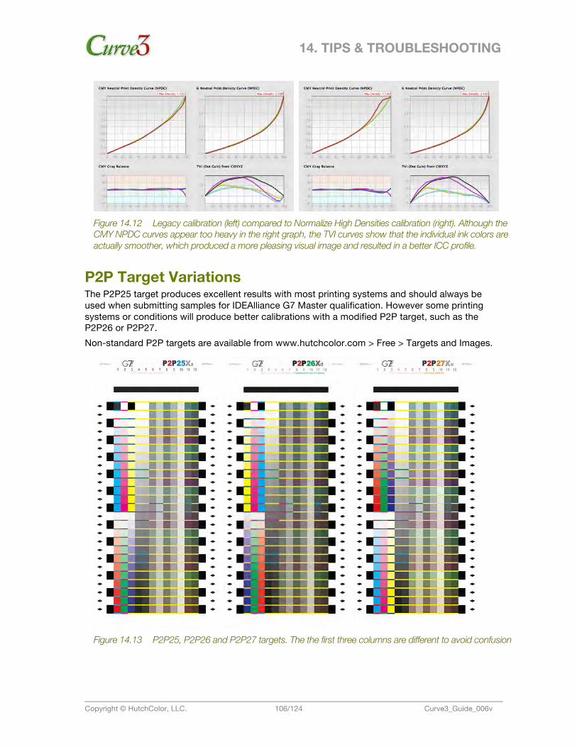
14. TIPS & TROUBLESHOOTING
Copyright © HutchColor, LLC. 106/124 Curve3_Guide_006v
Figure 14.12 Legacy calibration (left) compared to Normalize High Densities calibration (right). Although the CMY NPDC curves appear too heavy in the right graph, the TVI curves show that the individual ink colors are actually smoother, which produced a more pleasing visual image and resulted in a better ICC profile.
P2P Target Variations The P2P25 target produces excellent results with most printing systems and should always be used when submitting samples for IDEAlliance G7 Master qualification. However some printing systems or conditions will produce better calibrations with a modified P2P target, such as the P2P26 or P2P27. Non-standard P2P targets are available from www.hutchcolor.com > Free > Targets and Images.
Figure 14.13 P2P25, P2P26 and P2P27 targets. The the first three columns are different to avoid confusion
14. TIPS & TROUBLESHOOTING
Copyright © HutchColor, LLC. 107/124 Curve3_Guide_006v
P2P27 On some printing systems, especially wide-gamut ink jet, the gray balance of the first P2P is too far out for an accurate first calibration. Results may be improved either by iteration (See section 13) or by printing the P2P27 target instead of the P2P25.
CAUTION: When measuring the P2P27 you MUST use the correct P2P27 reference file.
P2P26 Indigo’s Basic color calibration system typically produces a very light print with zero dot gain (TVI). This means that when the P2P25 is printed, shadow balance is inaccurately measured, which can lead to less than ideal shadow balance correction. This can be solved by printing the P2P26 instead of the P2P25. The P2P26 target has a 16% TVI curve built in to it so the first print samples shadow gray balance more accurately.
CAUTION: When measuring the P2P26 you MUST use the correct P2P26 reference file.
P2P? Future P2P targets may be developed for special applications and will always have a unique identifier number. A higher-numbered P2P target does not necessarily replace the P2P25, but may be designed for special applications.
Mixed P2P Files Results will be incorrect if you combine measurements from two different types of P2P target, for example the P2P25 and P2P27. Make sure all measurement files are from the same P2P target.
USER GUIDE
Copyright © HutchColor, LLC. 108/124 Curve3_Guide_006v
Appendix: A. A. Target Printing This section discusses what you should know about printing targets for use with Curve3. Before performing a G7 calibration with Curve3 you must print at least one sample P2P target on the device you want to calibrate. If you plan on using the VPR (Virtual Press Run) module you must also print a characterization target, for example an HC2052F or an IT8.7/4, with the P2P.
Establishing a Base-line Condition Before attempting to calibrate a device with Curve3, be sure it is stable and in a repeatable ‘base-line’ condition. Record all variables for later reference. Base-line setup depends on the printing device, media selection and many other variables that a good operator should already be aware of. Only a few special situations will be discussed here.
Ink-limiting Most ink-jet printers require some form of ink-limiting to prevent excess ink being deposited on the substrate and causing drying problems. Proper ink-limiting settings should be established before printing the P2P target.
G7 calibration and ICC color management For maximum flexibility and value, G7 calibration should be performed with color management off. Once the device is calibrated, print a characterization target and create an ICC profile. In a perfect system Curve3’s calibration curves should be applied after color management is applied in the digital data flow. If color management cannot be switched off, but editorial tone curves are available in the RIP, print the P2P through an optimized color management setup then enter the G7 calibration into the editorial curves.
The P2P25 Target At the time of writing the preferred target for use with Curve3 is the P2P25. Two versions are available, the P2P25 and the P2P25Xa. Instructions for their use are in a ReadMe file in the P2P25 target package. The P2P25 target is available free at www.idealliance.com and can be downloaded from within Curve3 in the Web menu under Updates for P2P targets…
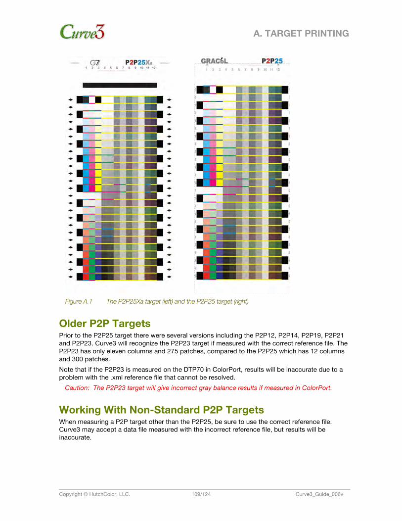
A. TARGET PRINTING
Copyright © HutchColor, LLC. 109/124 Curve3_Guide_006v
Figure A.1 The P2P25Xa target (left) and the P2P25 target (right)
Older P2P Targets Prior to the P2P25 target there were several versions including the P2P12, P2P14, P2P19, P2P21 and P2P23. Curve3 will recognize the P2P23 target if measured with the correct reference file. The P2P23 has only eleven columns and 275 patches, compared to the P2P25 which has 12 columns and 300 patches. Note that if the P2P23 is measured on the DTP70 in ColorPort, results will be inaccurate due to a problem with the .xml reference file that cannot be resolved.
Caution: The P2P23 target will give incorrect gray balance results if measured in ColorPort.
Working With Non-Standard P2P Targets When measuring a P2P target other than the P2P25, be sure to use the correct reference file. Curve3 may accept a data file measured with the incorrect reference file, but results will be inaccurate.
A. TARGET PRINTING
Copyright © HutchColor, LLC. 110/124 Curve3_Guide_006v
Custom-Generated and Odd-Size Targets If your measuring device or software does not work with the supplied targets, it may be possible to create a custom target (e.g. in X-Rite ColorPort, MeasureTool or i1Profiler) from a P2P definition file, but be aware of the following:
• Custom-generated target images MUST contain fractional percentage values, especially in light patches below 10%. Rounding fractional percentages to integers may lead to inaccurate G7 calibration.
• The supplied TIFF P2P targets use LSB (least significant bit) dithering to simulate better than 8-bit accuracy. This extra precision will normally be lost in custom-generated targets.
Printing the P2P Target For a new calibration, the P2P target should be printed in exactly the same way as normal work, but with no calibration curves present in the device RIP or driver. If calibrating a device with possible unevenness, for example an offset press, print at least two targets rotated 180° from each other and let Curve3 average both measurement sets. If the target will be measured on an X-Rite DTP70 or a X-Rite Eye One, be sure to print the target at exactly the same size as the file. If the target will be measured with an X-Rite i1iO or a hand-held device in spot mode, you can re-size or stretch the P2P target size to fit the measuring area.
Back-side printing Ideally, nothing should be printed on the reverse side of the P2P. If back-printing is unavoidable, either measure with black backing or make sure the reverse image is a flat tint of uniform color and density across the whole P2P area.
Printing Multiple P2P targets On devices with uneven ink coverage or other irregularities across the printing surface, at least two P2P targets should be printed in the same page, if space permits. On an offset or digital press, print as many targets as are practical and average them in Curve3. The Smooth function can improve calibration, even when multiple targets have been measured. On any device the best calibration curves are made by performing several G7 Calibration Runs over several days or weeks, and averaging the results.
Averaging Multiple Print Runs On printing systems whose performance varies significantly from run to run, such as offset lithography, screen printing, flexography and electro-photography (dry or wet toner), one Calibration Run is not enough to determine the average performance of that system over time. On any device the best calibration curves are made by performing several G7 Calibration Runs over several days or weeks, loading as many samples as you can from each run, then de-selecting any that don’t fit the average of the whole group. (See Measurement File Color Codes in Section 5.)
USER GUIDE
Copyright © HutchColor, LLC. 111/124 Curve3_Guide_006v
Appendix: B. B. Target Measuring This section discusses how to successfully measure targets for use with Curve3.
Measuring the P2P For detailed instructions on which reference files to use with different measuring devices, software and target versions, see the Read Me file in the P2P package.
Drying Time Most printing systems require some kind of drying or curing period before color and density are stabilized. Measuring a target before the drying time is complete may result in incorrect calibration curves. The same rule applies when measuring characterization data for Curve3’s VPR function. Before calibrating or profiling a printing system, find the correct drying time by measuring a P2P target immediately after it is printed, and then again after about 10 minutes, then 30 minutes, and if necessary up to 24 hours. Compare the gray balance and NPDC curves of the measurement files in the Measurements window. When measuring the same target multiple times, be careful not to scratch the surface or damage the target. Record the minimum drying time after which no change is observed and allow all future samples to dry at least that long before measuring them.
Coatings If you normally apply some kind of coating or finish material over the printed surface, for example aqueous or UV varnish in offset lithography or a laminate over ink-jet printing, apply the same finish to the P2P targets, and to any characterization targets when making profiles. If you sometimes apply the finish and sometimes do not, it is usually best to calibrate with the finish applied, then use the same RIP curves for both conditions. To determine if you need separate calibration curves for coated and un-coated printing, print a target (or series of targets) with and without coating, but with everything else the same, then compare the NPDC graphs and gray balance corrections suggested by Curve3. If they are nearly the same, use one common set of curves for both conditions.
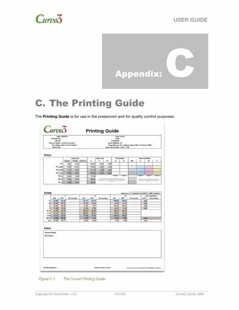
USER GUIDE
Copyright © HutchColor, LLC. 112/124 Curve3_Guide_006v
Appendix: C. C. The Printing Guide The Printing Guide is for use in the pressroom and for quality control purposes.
Figure C.1 The Curve3 Printing Guide
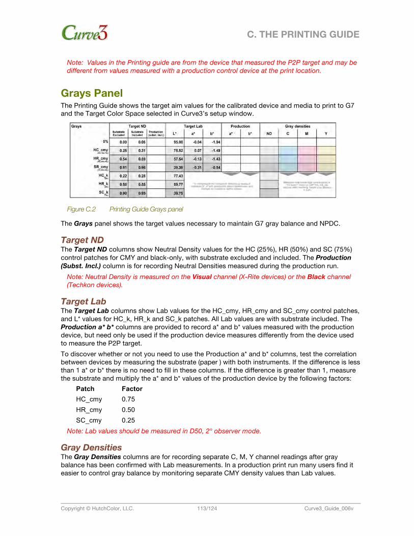
C. THE PRINTING GUIDE
Copyright © HutchColor, LLC. 113/124 Curve3_Guide_006v
Note: Values in the Printing guide are from the device that measured the P2P target and may be different from values measured with a production control device at the print location.
Grays Panel The Printing Guide shows the target aim values for the calibrated device and media to print to G7 and the Target Color Space selected in Curve3’s setup window.
Figure C.2 Printing Guide Grays panel
The Grays panel shows the target values necessary to maintain G7 gray balance and NPDC.
Target ND The Target ND columns show Neutral Density values for the HC (25%), HR (50%) and SC (75%) control patches for CMY and black-only, with substrate excluded and included. The Production (Subst. Incl.) column is for recording Neutral Densities measured during the production run.
Note: Neutral Density is measured on the Visual channel (X-Rite devices) or the Black channel (Techkon devices).
Target Lab The Target Lab columns show Lab values for the HC_cmy, HR_cmy and SC_cmy control patches, and L* values for HC_k, HR_k and SC_k patches. All Lab values are with substrate included. The Production a* b* columns are provided to record a* and b* values measured with the production device, but need only be used if the production device measures differently from the device used to measure the P2P target. To discover whether or not you need to use the Production a* and b* columns, test the correlation between devices by measuring the substrate (paper ) with both instruments. If the difference is less than 1 a* or b* there is no need to fill in these columns. If the difference is greater than 1, measure the substrate and multiply the a* and b* values of the production device by the following factors:
Patch Factor HC_cmy 0.75 HR_cmy 0.50 SC_cmy 0.25
Note: Lab values should be measured in D50, 2° observer mode.
Gray Densities The Gray Densities columns are for recording separate C, M, Y channel readings after gray balance has been confirmed with Lab measurements. In a production print run many users find it easier to control gray balance by monitoring separate CMY density values than Lab values.
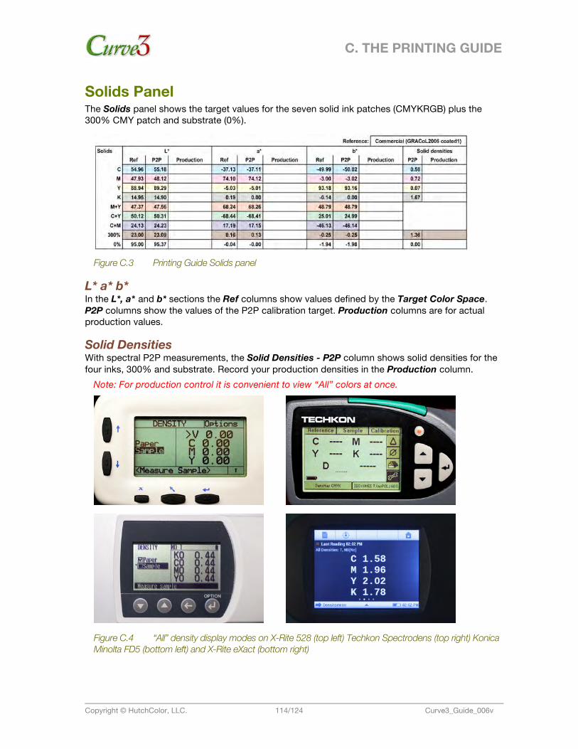
C. THE PRINTING GUIDE
Copyright © HutchColor, LLC. 114/124 Curve3_Guide_006v
Solids Panel The Solids panel shows the target values for the seven solid ink patches (CMYKRGB) plus the 300% CMY patch and substrate (0%).
Figure C.3 Printing Guide Solids panel
L* a* b* In the L*, a* and b* sections the Ref columns show values defined by the Target Color Space. P2P columns show the values of the P2P calibration target. Production columns are for actual production values.
Solid Densities With spectral P2P measurements, the Solid Densities - P2P column shows solid densities for the four inks, 300% and substrate. Record your production densities in the Production column.
Note: For production control it is convenient to view “All” colors at once.
Figure C.4 “All” density display modes on X-Rite 528 (top left) Techkon Spectrodens (top right) Konica Minolta FD5 (bottom left) and X-Rite eXact (bottom right)
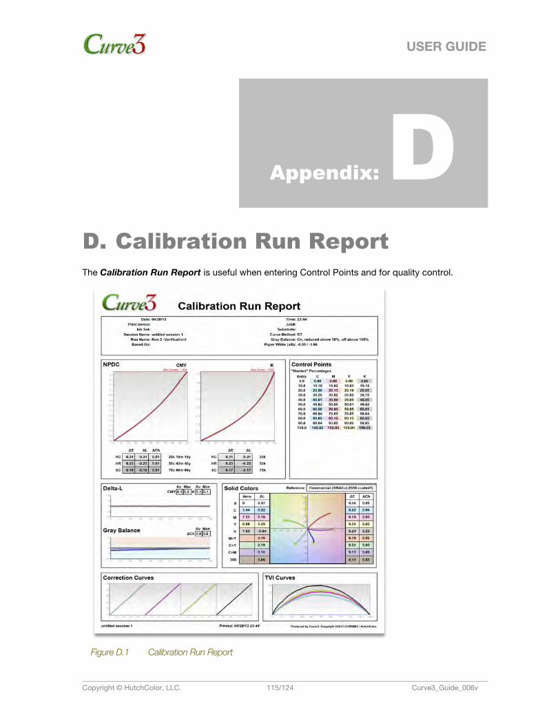
USER GUIDE
Copyright © HutchColor, LLC. 115/124 Curve3_Guide_006v
Appendix: D. D. Calibration Run Report The Calibration Run Report is useful when entering Control Points and for quality control.
Figure D.1 Calibration Run Report
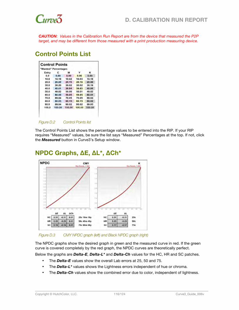
D. CALIBRATION RUN REPORT
Copyright © HutchColor, LLC. 116/124 Curve3_Guide_006v
CAUTION: Values in the Calibration Run Report are from the device that measured the P2P target, and may be different from those measured with a print production measuring device.
Control Points List
Figure D.2 Control Points list
The Control Points List shows the percentage values to be entered into the RIP. If your RIP requires “Measured” values, be sure the list says “Measured” Percentages at the top. If not, click the Measured button in Curve3’s Setup window.
NPDC Graphs, ∆E, ∆L*, ∆Ch*
Figure D.3 CMY NPDC graph (left) and Black NPDC graph (right)
The NPDC graphs show the desired graph in green and the measured curve in red. If the green curve is covered completely by the red graph, the NPDC curves are theoretically perfect. Below the graphs are Delta-E, Delta-L* and Delta-Ch values for the HC, HR and SC patches.
• The Delta-E values show the overall Lab errors at 25, 50 and 75. • The Delta-L* values shows the Lightness errors independent of hue or chroma. • The Delta-Ch values show the combined error due to color, independent of lightness.
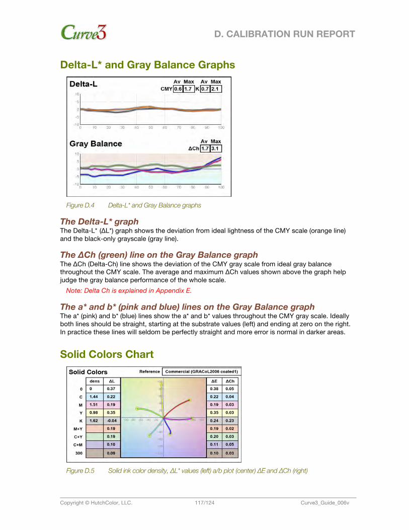
D. CALIBRATION RUN REPORT
Copyright © HutchColor, LLC. 117/124 Curve3_Guide_006v
Delta-L* and Gray Balance Graphs
Figure D.4 Delta-L* and Gray Balance graphs
The Delta-L* graph The Delta-L* (∆L*) graph shows the deviation from ideal lightness of the CMY scale (orange line) and the black-only grayscale (gray line).
The ∆Ch (green) line on the Gray Balance graph The ∆Ch (Delta-Ch) line shows the deviation of the CMY gray scale from ideal gray balance throughout the CMY scale. The average and maximum ∆Ch values shown above the graph help judge the gray balance performance of the whole scale.
Note: Delta Ch is explained in Appendix E.
The a* and b* (pink and blue) lines on the Gray Balance graph The a* (pink) and b* (blue) lines show the a* and b* values throughout the CMY gray scale. Ideally both lines should be straight, starting at the substrate values (left) and ending at zero on the right. In practice these lines will seldom be perfectly straight and more error is normal in darker areas.
Solid Colors Chart
Figure D.5 Solid ink color density, ∆L* values (left) a/b plot (center) ∆E and ∆Ch (right)
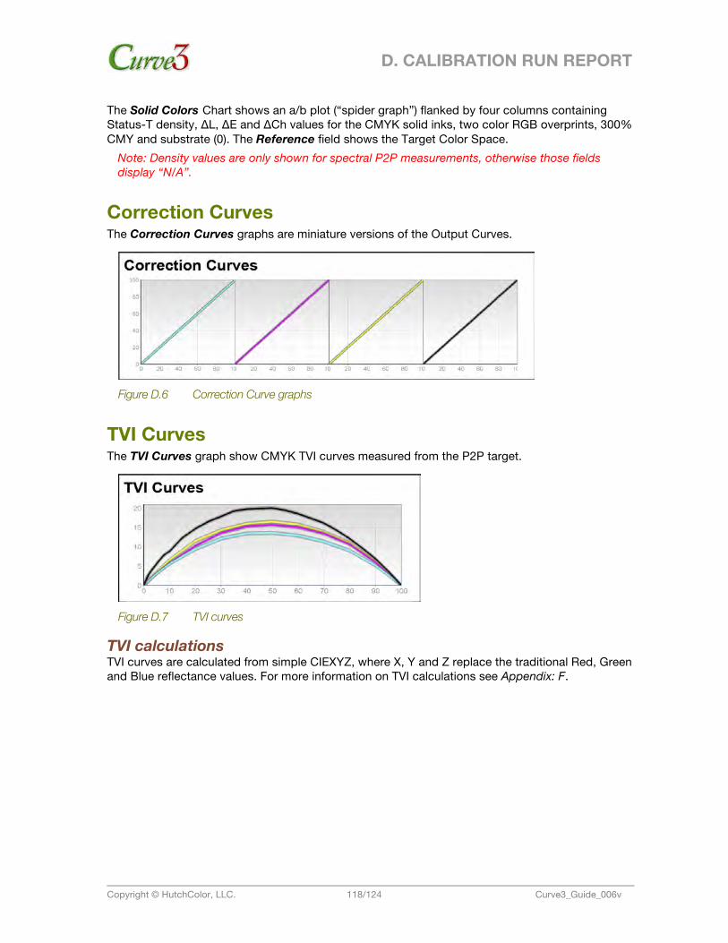
D. CALIBRATION RUN REPORT
Copyright © HutchColor, LLC. 118/124 Curve3_Guide_006v
The Solid Colors Chart shows an a/b plot (“spider graph”) flanked by four columns containing Status-T density, ∆L, ∆E and ∆Ch values for the CMYK solid inks, two color RGB overprints, 300% CMY and substrate (0). The Reference field shows the Target Color Space.
Note: Density values are only shown for spectral P2P measurements, otherwise those fields display “N/A”.
Correction Curves The Correction Curves graphs are miniature versions of the Output Curves.
Figure D.6 Correction Curve graphs
TVI Curves The TVI Curves graph show CMYK TVI curves measured from the P2P target.
Figure D.7 TVI curves
TVI calculations TVI curves are calculated from simple CIEXYZ, where X, Y and Z replace the traditional Red, Green and Blue reflectance values. For more information on TVI calculations see Appendix: F.
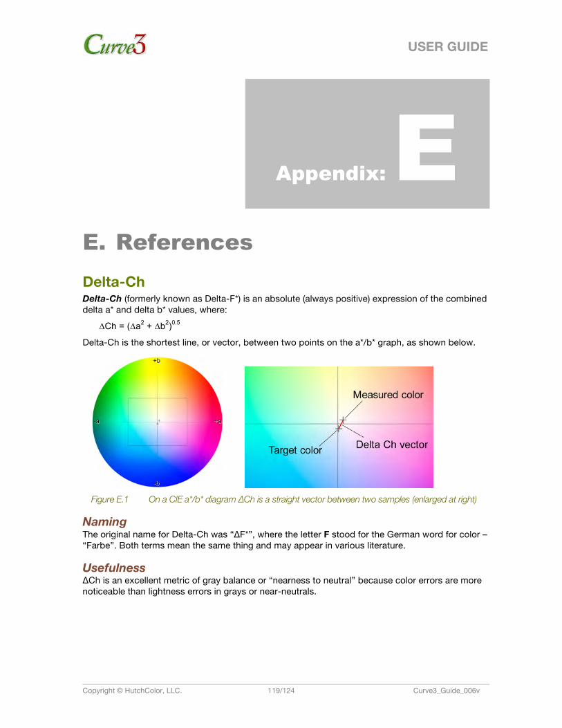
USER GUIDE
Copyright © HutchColor, LLC. 119/124 Curve3_Guide_006v
Appendix: E. E. References Delta-Ch Delta-Ch (formerly known as Delta-F*) is an absolute (always positive) expression of the combined delta a* and delta b* values, where:
∆Ch = (∆a2 + ∆b2)0.5
Delta-Ch is the shortest line, or vector, between two points on the a*/b* graph, as shown below.
Figure E.1 On a CIE a*/b* diagram ∆Ch is a straight vector between two samples (enlarged at right)
Naming The original name for Delta-Ch was “∆F*”, where the letter F stood for the German word for color – “Farbe”. Both terms mean the same thing and may appear in various literature.
Usefulness ∆Ch is an excellent metric of gray balance or “nearness to neutral” because color errors are more noticeable than lightness errors in grays or near-neutrals.
E. REFERENCES
Copyright © HutchColor, LLC. 120/124 Curve3_Guide_006v
Curve3 File Formats and Data Types File Formats Accepted by Curve3 Curve3 accepts most CGATS-standard files saved out of software from Barbieri, basICColor, Konica-Minolta, X-Rite, and others. Other file types are also accepted, for example the Logo file format exported from X-Rite MeasureTool™ and files exported from CHROMiX ColorThink™. Custom text files exported from an application like Microsoft Excel® will be accepted so long as each patch row contains both the printed CMYK values and the measured values in a separate row.
Colorimetric Data Types Accepted by Curve3 P2P measurement files may contain CIELAB, CIEXYZ and/or spectral data. When multiple data types are included in the same file, Curve3 uses them in the following order:
1. Spectral (first preference) 2. XYZ (second preference) 3. LAB (last preference)
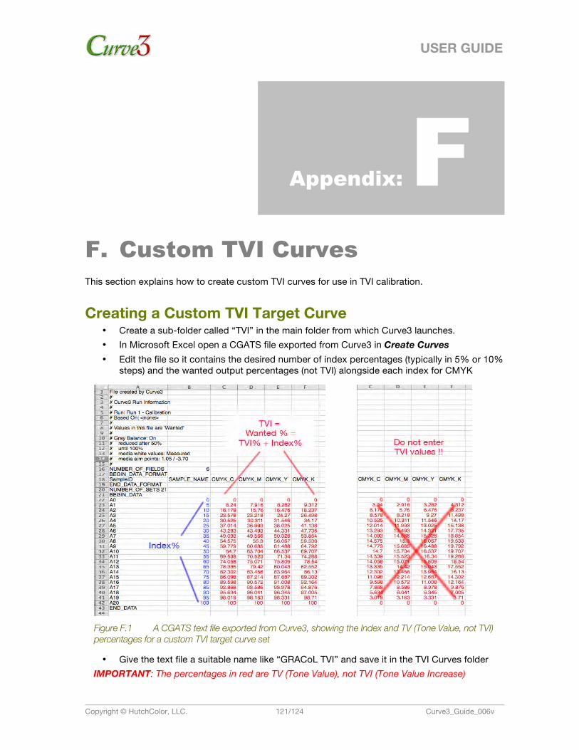
USER GUIDE
Copyright © HutchColor, LLC. 121/124 Curve3_Guide_006v
Appendix: F. F. Custom TVI Curves This section explains how to create custom TVI curves for use in TVI calibration.
Creating a Custom TVI Target Curve • Create a sub-folder called “TVI” in the main folder from which Curve3 launches. • In Microsoft Excel open a CGATS file exported from Curve3 in Create Curves • Edit the file so it contains the desired number of index percentages (typically in 5% or 10%
steps) and the wanted output percentages (not TVI) alongside each index for CMYK
Figure F.1 A CGATS text file exported from Curve3, showing the Index and TV (Tone Value, not TVI) percentages for a custom TVI target curve set
• Give the text file a suitable name like “GRACoL TVI” and save it in the TVI Curves folder IMPORTANT: The percentages in red are TV (Tone Value), not TVI (Tone Value Increase)
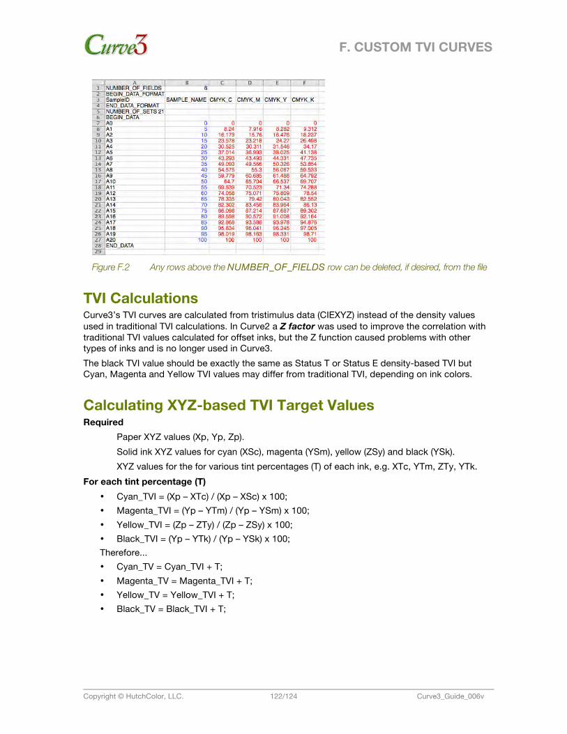
F. CUSTOM TVI CURVES
Copyright © HutchColor, LLC. 122/124 Curve3_Guide_006v
Figure F.2 Any rows above the NUMBER_OF_FIELDS row can be deleted, if desired, from the file
TVI Calculations Curve3’s TVI curves are calculated from tristimulus data (CIEXYZ) instead of the density values used in traditional TVI calculations. In Curve2 a Z factor was used to improve the correlation with traditional TVI values calculated for offset inks, but the Z function caused problems with other types of inks and is no longer used in Curve3. The black TVI value should be exactly the same as Status T or Status E density-based TVI but Cyan, Magenta and Yellow TVI values may differ from traditional TVI, depending on ink colors.
Calculating XYZ-based TVI Target Values Required
Paper XYZ values (Xp, Yp, Zp). Solid ink XYZ values for cyan (XSc), magenta (YSm), yellow (ZSy) and black (YSk). XYZ values for the for various tint percentages (T) of each ink, e.g. XTc, YTm, ZTy, YTk.
For each tint percentage (T) • Cyan_TVI = (Xp – XTc) / (Xp – XSc) x 100; • Magenta_TVI = (Yp – YTm) / (Yp – YSm) x 100; • Yellow_TVI = (Zp – ZTy) / (Zp – ZSy) x 100; • Black_TVI = (Yp – YTk) / (Yp – YSk) x 100; Therefore... • Cyan_TV = Cyan_TVI + T; • Magenta_TV = Magenta_TVI + T; • Yellow_TV = Yellow_TVI + T; • Black_TV = Black_TVI + T;

USER GUIDE
Copyright © HutchColor, LLC. 123/124 Curve3_Guide_006v
Appendix: G. G. G7 Via Color Management This section explains how to pass the IDEAlliance G7 Master requirements on a printing system that doesn’t accept calibration curves.
No RIP Curves? If your RIP or printing system doesn’t allow you to enter custom calibration curves, you may not be able to use a normal Curve3 calibration, but you can still simulate the appearance of G7 calibration via color management, as follows:
• Calibrate the system by the manufacturer’s method, or by whatever means are available • Create an ICC profile of the system, or use the system’s proprietary color management • Assign a G7-based ICC profile such as GRACoL2006_Coated1v2.icc, or assign a
Reference Print Condition (RPC) based on G7 or CGATS TR015 • Set the rendering intent to Absolute or Relative Colorimetric (Perceptual is not
recommended) • Print the P2P25 target through the workflow • Measure the P2P target and load the in Curve3’s Verify window • Check the G7 Pass/Fail condition. If all number fields are green, the system is in G7
compliance
Limitations Although this method will simulate G7 and can be used to IDEAlliance “G7 Master” status, you will not be getting the full benefit of G7 calibration. For example:
• You must always use a source profile, so you won’t be able to capitalize on the maximum ink saturation of your device for a “G7 Extreme” effect
• You lose Curve3’s ability to fine-tune gray balance and tonality in very light tones • You must re-create a new output profile every time the system changes, whereas in a G7-
based system a quick re-calibration can often maintain the value of your original profile
G. G7 VIA COLOR MANAGEMENT
Copyright © HutchColor, LLC. 124/124 Curve3_Guide_006v
G7-Based Reference Print Conditions TR015 The CGATS Technical Report “TR015” constitutes a formal definition of G7. IDEAlliance members can learn about TR015 at www.idealliance.org. Any characterization data based on CGATS TR015 is effectively “G7-based”. The most common G7-based data sets are GRACoL 2006, SWOP3 2006 and SWOP5 2006.
CGATS.21 In 2013 the American National Standards Institute (ANSI) accepted a set of seven standardized Reference Print Conditions (RPCs) published under the group name CGATS.21, that are based on TR015. These data sets cover a wide range of printing conditions from cold-set newsprint to extended gamut offset. More information on CGATS.21 and TR015 can be found at www.NPES.org. Seven free ICC profiles based on CGATS.21 are available at www.idealliance.org.
Note: For copyright reasons, neither HutchColor nor CHROMiX can provide these documents or the CGATS.21 RPC data sets or ICC profiles.