curtis/courses/PhD-PVT/PVT-HOT-Vienna-May-2016x/e...18 PHASE BEHAVIOR Chap. 3 covers the properties...
29
18 PHASE BEHAVIOR Chapter 3 Gas and Oil Properties and Correlations 3.1 Introduction Chap. 3 covers the properties of oil and gas systems, their nomencla- ture and units, and correlations used for their prediction. Sec. 3.2 covers the fundamental engineering quantities used to describe phase behavior, including molecular quantities, critical and reduced properties, component fractions, mixing rules, volumetric proper- ties, transport properties, and interfacial tension (IFT). Sec. 3.3 discusses the properties of gas mixtures, including cor- relations for Z factor, pseudocritical properties and wellstream grav- ity, gas viscosity, dewpoint pressure, and total formation volume factor (FVF). Sec. 3.4 covers oil properties, including correlations for bubblepoint pressure, compressibility, FVF, density, and viscos- ity. Sec. 3.5 gives correlations for IFT and diffusion coefficients. Sec. 3.6 reviews the estimation of K values for low-pressure ap- plications, such as surface separator design, and convergence-pres- sure methods used for reservoir calculations. 3.2 Review of Properties, Nomenclature, and Units 3.2.1 Molecular Quantities. All matter is composed of elements that cannot be decomposed by ordinary chemical reactions. Carbon (C), hydrogen (H), sulfur (S), nitrogen (N), and oxygen (O) are examples of the elements found in naturally occurring petroleum systems. The physical unit of the element is the atom. Two or more ele- ments may combine to form a chemical compound. Carbon dioxide (CO 2 ), methane (CH 4 ), and hydrogen sulfide (H 2 S) are examples of compounds found in naturally occurring petroleum systems. When two atoms of the same element combine, they form diatomic com- pounds, such as nitrogen (N 2 ) and oxygen (O 2 ). The physical unit of the compound is the molecule. Mass is the basic quantity for measuring the amount of a substance. Because chemical compounds always combine in a definite propor- tion (i.e., as a simple ratio of whole numbers), the mass of the atoms of different elements can be conveniently compared by relating them with a standard. The current standard is carbon-12, where the element carbon has been assigned a relative atomic mass of 12.011. The relative atomic mass of all other elements have been deter- mined relative to the carbon-12 standard. The smallest element is hydrogen, which has a relative atomic mass of 1.0079. The relative atomic mass of one element contains the same number of atoms as the relative atomic mass of any other element. This is true regardless of the units used to measure mass. According to the SI standard, the definition of the mole reads “the mole is the amount of substance of a system which contains as many elementary entities as there are atoms in 0.012 kilograms of car- bon-12.” The SI symbol for mole is mol, which is numerically iden- tical to the traditional g mol. The SPE SI standard 1 uses kmol as the unit for a mole where kmol designates “an amount of substance which contains as many kilo- grams (groups of molecules) as there are atoms in 12.0 kg (incor- rectly written as 0.012 kg in the original SPE publication) of car- bon-12 multiplied by the relative molecular mass of the substance involved.” A practical way to interpret kmol is “kg mol” where kmol is nu- merically equivalent to 1,000 g mol (i.e., 1,000 mol). Otherwise, the following conversions apply. 1 kmol + 1,000 mol + 1,000 g mol + 2.2046 lbm mol 1 lbm mol + 0.45359 kmol + 453.59 mol + 453.59 g mol 1 mol + 1 g mol + 0.001 kmol + 0.0022046 lbm mol The term molecular weight has been replaced in the SI system by molar mass. Molar mass, M, is defined as the mass per mole (M+m/n) of a given substance where the unit mole must be consis- tent with the unit of mass. The numerical value of molecular weight is independent of the units used for mass and moles, as long as the units are consistent. For example, the molar mass of methane is 16.04, which for various units can be written M+ 16.04 kg/kmol + 16.04 lbm/lbm mol + 16.04 g/g mol + 16.04 g/mol 3.2.2 Critical and Reduced Properties. Most equations of state (EOS’s) do not use pressure and temperature explicitly to define the state of a system, but instead they generalize according to corre- sponding-states theory by use of two or more reduced properties, which are dimensionless. 2 T r + TńT c , (3.1a) . . . . . . . . . . . . . . . . . . . . . . . . . . . . . . . . . . .
Transcript of curtis/courses/PhD-PVT/PVT-HOT-Vienna-May-2016x/e...18 PHASE BEHAVIOR Chap. 3 covers the properties...

18 PHASE BEHAVIOR
������� �
� ��� �� ��������� ��� �����������
��� ������������
Chap. 3 covers the properties of oil and gas systems, their nomencla-ture and units, and correlations used for their prediction. Sec. 3.2covers the fundamental engineering quantities used to describephase behavior, including molecular quantities, critical and reducedproperties, component fractions, mixing rules, volumetric proper-ties, transport properties, and interfacial tension (IFT).
Sec. 3.3 discusses the properties of gas mixtures, including cor-relations for Z factor, pseudocritical properties and wellstream grav-ity, gas viscosity, dewpoint pressure, and total formation volumefactor (FVF). Sec. 3.4 covers oil properties, including correlationsfor bubblepoint pressure, compressibility, FVF, density, and viscos-ity. Sec. 3.5 gives correlations for IFT and diffusion coefficients.Sec. 3.6 reviews the estimation of K values for low-pressure ap-plications, such as surface separator design, and convergence-pres-sure methods used for reservoir calculations.
��� ������ �� ���������� ������������� ��� ����
3.2.1 Molecular Quantities. All matter is composed of elements thatcannot be decomposed by ordinary chemical reactions. Carbon (C),hydrogen (H), sulfur (S), nitrogen (N), and oxygen (O) are examplesof the elements found in naturally occurring petroleum systems.
The physical unit of the element is the atom. Two or more ele-ments may combine to form a chemical compound. Carbon dioxide(CO2), methane (CH4), and hydrogen sulfide (H2S) are examples ofcompounds found in naturally occurring petroleum systems. Whentwo atoms of the same element combine, they form diatomic com-pounds, such as nitrogen (N2) and oxygen (O2). The physical unitof the compound is the molecule.
Mass is the basic quantity for measuring the amount of a substance.Because chemical compounds always combine in a definite propor-tion (i.e., as a simple ratio of whole numbers), the mass of the atomsof different elements can be conveniently compared by relating themwith a standard. The current standard is carbon-12, where the elementcarbon has been assigned a relative atomic mass of 12.011.
The relative atomic mass of all other elements have been deter-mined relative to the carbon-12 standard. The smallest element ishydrogen, which has a relative atomic mass of 1.0079. The relativeatomic mass of one element contains the same number of atoms asthe relative atomic mass of any other element. This is true regardlessof the units used to measure mass.
According to the SI standard, the definition of the mole reads “themole is the amount of substance of a system which contains as manyelementary entities as there are atoms in 0.012 kilograms of car-
bon-12.” The SI symbol for mole is mol, which is numerically iden-tical to the traditional g mol.
The SPE SI standard1 uses kmol as the unit for a mole where kmoldesignates “an amount of substance which contains as many kilo-grams (groups of molecules) as there are atoms in 12.0 kg (incor-rectly written as 0.012 kg in the original SPE publication) of car-bon-12 multiplied by the relative molecular mass of the substanceinvolved.”
A practical way to interpret kmol is “kg mol” where kmol is nu-merically equivalent to 1,000 g mol (i.e., 1,000 mol). Otherwise, thefollowing conversions apply.
1 kmol � 1,000 mol� 1,000 g mol� 2.2046 lbm mol
1 lbm mol � 0.45359 kmol� 453.59 mol� 453.59 g mol
1 mol � 1 g mol� 0.001 kmol� 0.0022046 lbm mol
The term molecular weight has been replaced in the SI system bymolar mass. Molar mass, M, is defined as the mass per mole(M�m/n) of a given substance where the unit mole must be consis-tent with the unit of mass. The numerical value of molecular weightis independent of the units used for mass and moles, as long as theunits are consistent. For example, the molar mass of methane is16.04, which for various units can be written
M� 16.04 kg/kmol� 16.04 lbm/lbm mol� 16.04 g/g mol� 16.04 g/mol
3.2.2 Critical and Reduced Properties. Most equations of state(EOS’s) do not use pressure and temperature explicitly to define thestate of a system, but instead they generalize according to corre-sponding-states theory by use of two or more reduced properties,which are dimensionless.2
Tr� T�Tc , (3.1a). . . . . . . . . . . . . . . . . . . . . . . . . . . . . . . . . . .
GAS AND OIL PROPERTIES AND CORRELATIONS 19
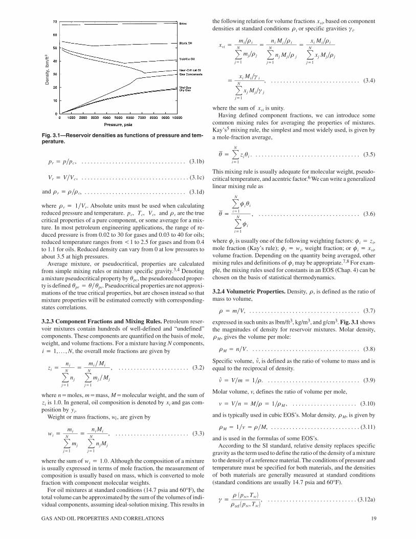
Fig. 3.1—Reservoir densities as functions of pressure and tem-perature.
pr� p�pc , (3.1b). . . . . . . . . . . . . . . . . . . . . . . . . . . . . . . . . .
Vr� V�Vc , (3.1c). . . . . . . . . . . . . . . . . . . . . . . . . . . . . . . . . . .
and �r� ���c, (3.1d). . . . . . . . . . . . . . . . . . . . . . . . . . . . . . . . .
where �r� 1�Vr. Absolute units must be used when calculatingreduced pressure and temperature. pc, Tc, Vc, and �c are the truecritical properties of a pure component, or some average for a mix-ture. In most petroleum engineering applications, the range of re-duced pressure is from 0.02 to 30 for gases and 0.03 to 40 for oils;reduced temperature ranges from �1 to 2.5 for gases and from 0.4to 1.1 for oils. Reduced density can vary from 0 at low pressures toabout 3.5 at high pressures.
Average mixture, or pseudocritical, properties are calculatedfrom simple mixing rules or mixture specific gravity.3,4 Denotinga mixture pseudocritical property by �pc, the pseudoreduced proper-ty is defined �pr� ���pc. Pseudocritical properties are not approxi-mations of the true critical properties, but are chosen instead so thatmixture properties will be estimated correctly with corresponding-states correlations.
3.2.3 Component Fractions and Mixing Rules. Petroleum reser-voir mixtures contain hundreds of well-defined and “undefined”components. These components are quantified on the basis of mole,weight, and volume fractions. For a mixture having N components,i� 1, . . . , N, the overall mole fractions are given by
zi�ni
�N
j�1
nj
�mi�Mi
�N
j�1
mj�Mj
, (3.2). . . . . . . . . . . . . . . . . . . . . . .
where n�moles, m�mass, M�molecular weight, and the sum ofzi is 1.0. In general, oil composition is denoted by xi and gas com-position by yi.
Weight or mass fractions, wi, are given by
wi�mi
�N
j�1
mj
�ni Mi
�N
j�1
nj Mj
, (3.3). . . . . . . . . . . . . . . . . . . . . . . .
where the sum of wi� 1.0. Although the composition of a mixtureis usually expressed in terms of mole fraction, the measurement ofcomposition is usually based on mass, which is converted to molefraction with component molecular weights.
For oil mixtures at standard conditions (14.7 psia and 60°F), thetotal volume can be approximated by the sum of the volumes of indi-vidual components, assuming ideal-solution mixing. This results in
the following relation for volume fractions xvi, based on componentdensities at standard conditions �i or specific gravities �i.
xvi�mi��i
�N
j�1
mj��j
�ni Mi��i
�N
j�1
nj Mj�� j
�xi Mi��i
�N
j�1
xj Mj��j
�xi Mi�� i
�N
j�1
xj Mj�� j
, (3.4). . . . . . . . . . . . . . . . . . . . . . . . . . . . .
where the sum of xvi is unity.Having defined component fractions, we can introduce some
common mixing rules for averaging the properties of mixtures.Kay’s5 mixing rule, the simplest and most widely used, is given bya mole-fraction average,
���N
i�1
zi�i . (3.5). . . . . . . . . . . . . . . . . . . . . . . . . . . . . . . . . .
This mixing rule is usually adequate for molecular weight, pseudo-critical temperature, and acentric factor.6 We can write a generalizedlinear mixing rule as
��
��
N
i�1i�i
�N
i�1
�i
, (3.6). . . . . . . . . . . . . . . . . . . . . . . . . . . . . . . . .
where �i is usually one of the following weighting factors: �i� zi,mole fraction (Kay’s rule); �i� wi, weight fraction; or �i� xvi,volume fraction. Depending on the quantity being averaged, othermixing rules and definitions of �i may be appropriate.7,8 For exam-ple, the mixing rules used for constants in an EOS (Chap. 4) can bechosen on the basis of statistical thermodynamics.
3.2.4 Volumetric Properties. Density, �, is defined as the ratio ofmass to volume,
�� m�V, (3.7). . . . . . . . . . . . . . . . . . . . . . . . . . . . . . . . . . . .
expressed in such units as lbm/ft3, kg/m3, and g/cm3. Fig. 3.1 showsthe magnitudes of density for reservoir mixtures. Molar density,�M, gives the volume per mole:
�M� n�V. (3.8). . . . . . . . . . . . . . . . . . . . . . . . . . . . . . . . . . .
Specific volume, v^, is defined as the ratio of volume to mass and isequal to the reciprocal of density.
v^ � V�m� 1��. (3.9). . . . . . . . . . . . . . . . . . . . . . . . . . . . . .
Molar volume, v, defines the ratio of volume per mole,
v� V�n� M��� 1��M , (3.10). . . . . . . . . . . . . . . . . . . . .
and is typically used in cubic EOS’s. Molar density, �M, is given by
�M� 1�v� ��M, (3.11). . . . . . . . . . . . . . . . . . . . . . . . . . . . .
and is used in the formulas of some EOS’s.According to the SI standard, relative density replaces specific
gravity as the term used to define the ratio of the density of a mixtureto the density of a reference material. The conditions of pressure andtemperature must be specified for both materials, and the densitiesof both materials are generally measured at standard conditions(standard conditions are usually 14.7 psia and 60°F).
��� �psc, Tsc�
�ref�psc, Tsc�
, (3.12a). . . . . . . . . . . . . . . . . . . . . . . . . . . . .
20 PHASE BEHAVIOR
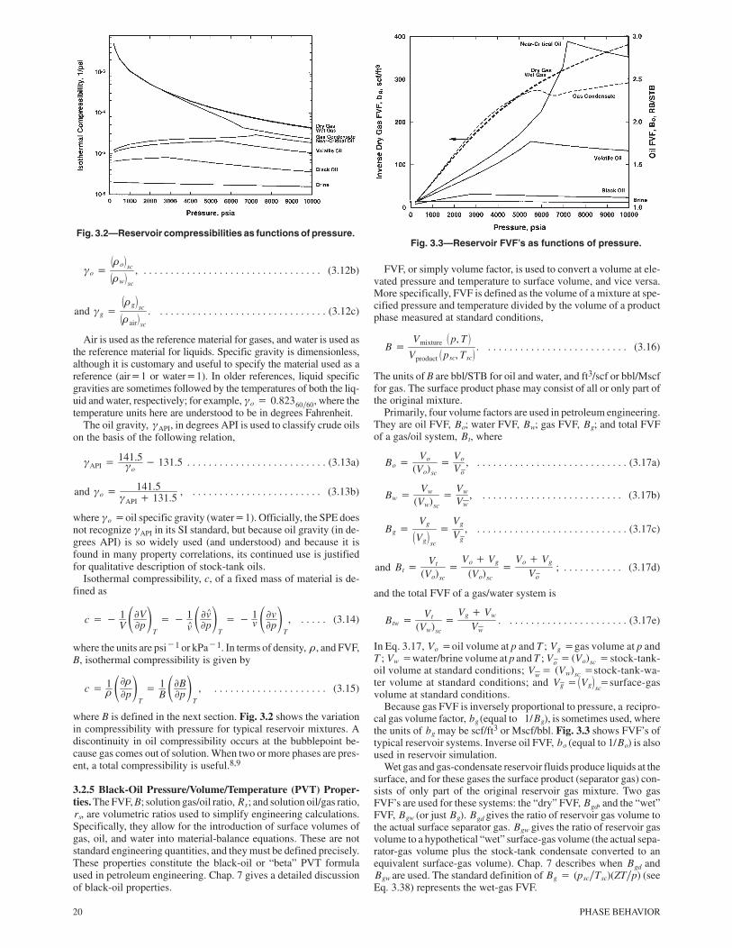
Fig. 3.2—Reservoir compressibilities as functions of pressure.
�o���o�sc
��w�sc
, (3.12b). . . . . . . . . . . . . . . . . . . . . . . . . . . . . . . . .
and �g���g�sc
��air�sc
. (3.12c). . . . . . . . . . . . . . . . . . . . . . . . . . . . . . .
Air is used as the reference material for gases, and water is used asthe reference material for liquids. Specific gravity is dimensionless,although it is customary and useful to specify the material used as areference (air�1 or water�1). In older references, liquid specificgravities are sometimes followed by the temperatures of both the liq-uid and water, respectively; for example, �o� 0.82360�60, where thetemperature units here are understood to be in degrees Fahrenheit.
The oil gravity, �API, in degrees API is used to classify crude oilson the basis of the following relation,
�API�141.5�o� 131.5 (3.13a). . . . . . . . . . . . . . . . . . . . . . . . . .
and �o�141.5
�API� 131.5, (3.13b). . . . . . . . . . . . . . . . . . . . . . . .
where �o�oil specific gravity (water�1). Officially, the SPE doesnot recognize �API in its SI standard, but because oil gravity (in de-grees API) is so widely used (and understood) and because it isfound in many property correlations, its continued use is justifiedfor qualitative description of stock-tank oils.
Isothermal compressibility, c, of a fixed mass of material is de-fined as
c�� 1V�Vp�
T
�� 1v^�v^p�
T
�� 1v �vp�
T
, (3.14). . . . .
where the units are psi�1 or kPa�1. In terms of density, �, and FVF,B, isothermal compressibility is given by
c� 1���p�
T
� 1B�Bp�
T
, (3.15). . . . . . . . . . . . . . . . . . . . .
where B is defined in the next section. Fig. 3.2 shows the variationin compressibility with pressure for typical reservoir mixtures. Adiscontinuity in oil compressibility occurs at the bubblepoint be-cause gas comes out of solution. When two or more phases are pres-ent, a total compressibility is useful.8,9
3.2.5 Black-Oil Pressure/Volume/Temperature (PVT) Proper-ties. The FVF, B; solution gas/oil ratio, Rs; and solution oil/gas ratio,rs, are volumetric ratios used to simplify engineering calculations.Specifically, they allow for the introduction of surface volumes ofgas, oil, and water into material-balance equations. These are notstandard engineering quantities, and they must be defined precisely.These properties constitute the black-oil or “beta” PVT formulaused in petroleum engineering. Chap. 7 gives a detailed discussionof black-oil properties.
Fig. 3.3—Reservoir FVF’s as functions of pressure.
FVF, or simply volume factor, is used to convert a volume at ele-vated pressure and temperature to surface volume, and vice versa.More specifically, FVF is defined as the volume of a mixture at spe-cified pressure and temperature divided by the volume of a productphase measured at standard conditions,
B�Vmixture
�p, T �
Vproduct�psc, Tsc�
. (3.16). . . . . . . . . . . . . . . . . . . . . . . . . .
The units of B are bbl/STB for oil and water, and ft3/scf or bbl/Mscffor gas. The surface product phase may consist of all or only part ofthe original mixture.
Primarily, four volume factors are used in petroleum engineering.They are oil FVF, Bo; water FVF, Bw; gas FVF, Bg; and total FVFof a gas/oil system, Bt, where
Bo�Vo
(Vo)sc�
Vo
Vo, (3.17a). . . . . . . . . . . . . . . . . . . . . . . . . . . .
Bw�Vw
(Vw)sc�
Vw
Vw, (3.17b). . . . . . . . . . . . . . . . . . . . . . . . . .
Bg�Vg
�Vg�sc
�Vg
Vg, (3.17c). . . . . . . . . . . . . . . . . . . . . . . . . . . .
and Bt�Vt
(Vo)sc�
Vo� Vg
(Vo)sc�
Vo� Vg
Vo; (3.17d). . . . . . . . . . .
and the total FVF of a gas/water system is
Btw�Vt
(Vw)sc�
Vg� Vw
Vw. (3.17e). . . . . . . . . . . . . . . . . . . . . .
In Eq. 3.17, Vo�oil volume at p and T ; Vg�gas volume at p andT ; Vw�water/brine volume at p and T ; Vo�(Vo)sc�stock-tank-oil volume at standard conditions; Vw� (Vw)sc�stock-tank-wa-ter volume at standard conditions; and Vg��Vg�sc
�surface-gasvolume at standard conditions.
Because gas FVF is inversely proportional to pressure, a recipro-cal gas volume factor, bg (equal to 1/Bg), is sometimes used, wherethe units of bg may be scf/ft3 or Mscf/bbl. Fig. 3.3 shows FVF’s oftypical reservoir systems. Inverse oil FVF, bo (equal to 1/Bo) is alsoused in reservoir simulation.
Wet gas and gas-condensate reservoir fluids produce liquids at thesurface, and for these gases the surface product (separator gas) con-sists of only part of the original reservoir gas mixture. Two gasFVF’s are used for these systems: the “dry” FVF, Bgd, and the “wet”FVF, Bgw (or just Bg). Bgd gives the ratio of reservoir gas volume tothe actual surface separator gas. Bgw gives the ratio of reservoir gasvolume to a hypothetical “wet” surface-gas volume (the actual sepa-rator-gas volume plus the stock-tank condensate converted to anequivalent surface-gas volume). Chap. 7 describes when Bgd andBgw are used. The standard definition of Bg� (psc�Tsc)(ZT�p) (seeEq. 3.38) represents the wet-gas FVF.

GAS AND OIL PROPERTIES AND CORRELATIONS 21
Fig. 3.4—Solution gas/oil ratios for brine, Rsw, and reservoir oils,Rs , and inverse solution oil/gas ratio for reservoir gases, 1/rs , asfunctions of pressure.
When a reservoir mixture produces both surface gas and oil, theGOR, Rgo, defines the ratio of standard gas volume to a referenceoil volume (stock-tank- or separator-oil volume),
Rgo��Vg�sc
(Vo)sc�
Vg
Vo(3.18a). . . . . . . . . . . . . . . . . . . . . . . . . . . .
and Rsp��Vg�sc
(Vo)sp�
Vg
(Vo)sp(3.18b). . . . . . . . . . . . . . . . . . . . . .
in units of scf/STB and scf/bbl, respectively. The separator condi-tions should be reported when separator GOR is used.
Solution gas/oil ratio, Rs, is the volume of gas (at standard condi-tions) liberated from a single-phase oil at elevated pressure and tem-perature divided by the resulting stock-tank-oil volume, with unitsscf/STB. Rs is constant at pressures greater than the bubblepoint anddecreases as gas is liberated at pressures below the bubblepoint.
The producing GOR, Rp, defines the instantaneous ratio of the to-tal surface-gas volume produced divided by the total stock-tank-oilvolume. At pressures greater than bubblepoint, Rp is constant andequal to Rs at bubblepoint. At pressures less than the bubblepoint,Rp may be equal to, less than, or greater than the Rs of the flowingreservoir oil. Typically, Rp will increase 10 to 20 times the initial Rs
because of increasing gas mobility and decreasing oil mobility dur-ing pressure depletion.
The surface volume ratio for gas condensates is usually expressedas an oil/gas ratio (OGR), rog.
rog�(Vo)sc
�Vg�sc
�Vo
Vg� 1
Rgo. (3.19). . . . . . . . . . . . . . . . . . . . . .
The unit for rog is STB/scf or, more commonly, “barrels per million”(STB/MMscf). To avoid misinterpretation, it should be clearly spe-cified whether the OGR includes natural gas liquids (NGL’s) inaddition to stock-tank condensate. In most petroleum engineeringcalculations, NGL’s are not included in the OGR.
The ratio of surface oil to surface gas produced from a single-phase reservoir gas is referred to as the solution oil/gas ratio, rs. Atpressures above the dewpoint, the producing OGR, rp is constantand equal to rs at the dewpoint. At pressures below the dewpoint, rp
is typically equal to or just slightly greater than rs; the contributionof flowing reservoir oil to surface-oil production is negligible inmost gas-condensate reservoirs.
In the definitions of Rp and rp, the total producing surface-gasvolume equals the surface gas from the reservoir gas plus the solu-tion gas from the reservoir oil; likewise, the total producing surfaceoil equals the stock-tank oil from the reservoir oil plus the conden-sate from the reservoir gas. Fig. 3.4 shows the behavior of Rp, Rs,and 1�rs as a function of pressure.
Fig. 3.5—Reservoir viscosities as functions of pressure.
3.2.6 Viscosity. Two types of viscosity are used in engineering cal-culations: dynamic viscosity, �� and kinematic viscosity, �. The def-inition of � for Newtonian flow (which most petroleum mixturesfollow) is
���gc
du�dy, (3.20). . . . . . . . . . . . . . . . . . . . . . . . . . . . . . . . .
where ��shear stress per unit area in the shear plane parallel to thedirection of flow, du/dy�velocity gradient perpendicular to theplane of shear, and gc�a units conversion from mass to force. Thetwo viscosities are related by density, where ��� �.
Most petroleum engineering applications use dynamic viscosity,which is the property reported in commercial laboratory studies.The unit of dynamic viscosity is centipoise (cp), or in SI units,mPas, where 1 cp�1 mPas. Kinematic viscosity is usually re-ported in centistoke (cSt), which is obtained by dividing � in cp by� in g/cm3; the SI unit for � is mm2/s, which is numerically equiva-lent to centistoke. Fig. 3.5 shows oil, gas, and water viscosities fortypical reservoir systems.
3.2.7 Diffusion Coefficients. In the absence of bulk flow, compo-nents in a single-phase mixture are transported according to gradi-ents in concentration (i.e., chemical potential). Fick’s10 law for 1Dmolecular diffusion in a binary system is given by
ui�� Di j�dCi�dx�, (3.21). . . . . . . . . . . . . . . . . . . . . . . . . .
where ui�molar velocity of Component i; Dij�binary diffusioncoefficient; and Ci�molar concentration of Component i� yi�M,where yi�mole fraction; and x�distance.
Eq. 3.21 clearly shows that mass transfer by molecular diffusioncan be significant for three reasons: (1) large diffusion coefficients,(2) large concentration differences, and (3) short distances. A com-bination of moderate diffusion coefficients, concentration gradi-ents, and distance may also result in significant diffusive flow. Mo-lecular diffusion is particularly important in naturally fracturedreservoirs11,12 because of relatively short distances (e.g., small ma-trix block sizes).
Low-pressure binary diffusion coefficients for gases, Doij, are in-
dependent of composition and can be calculated accurately fromfundamental gas theory (Chapman and Enskog6), which are basical-ly the same relations used to estimate low-pressure gas viscosity. Nowell-accepted method is available to correct Do
ij for mixtures at highpressure, but two types of corresponding-states correlations havebeen proposed: Dij� Do
ij f(Tr, pr) and Dij� Doij f(�r).
At low pressures, diffusion coefficients are several orders of mag-nitude smaller in liquids than in gases. At reservoir conditions, thedifference between gas and liquid diffusion coefficients may be lessthan one order of magnitude.
3.2.8 IFT. Interfacial forces act between equilibrium gas, oil, andwater phases coexisting in the pores of a reservoir rock. These forces

22 PHASE BEHAVIOR
are generally quantified in terms of IFT, �� units of � are dynes/cm(or equivalently, mN/m). The magnitude of IFT varies from �50dynes/cm for crude-oil/gas systems at standard conditions to �0.1dyne/cm for high-pressure gas/oil mixtures. Gas/oil capillary pres-sure, Pc, is usually considered proportional to IFT according to theYoung-Laplace equation Pc� 2��r, where r is an average pore ra-dius.13-15 Recovery mechanisms that are influenced by capillarypressure (e.g., gas injection in naturally fractured reservoirs) willnecessarily be sensitive to IFT.
��� � �!����
This section gives correlations for PVT properties of natural gases,including the following.
1. Review of gas volumetric properties.2. Z-factor correlations.3. Gas pseudocritical properties.4. Wellstream gravity of wet gases and gas condensates.5. Gas viscosity.6. Dewpoint pressure.7. Total volume factor.
3.3.1 Review of Gas Volumetric Properties. The properties of gasmixtures are well understood and have been accurately correlatedfor many years with graphical charts and EOS’s based on extensiveexperimental data.16-19 The behavior of gases at low pressures wasoriginally quantified on the basis of experimental work by Charlesand Boyle, which resulted in the ideal-gas law,3
pV� nRT, (3.22). . . . . . . . . . . . . . . . . . . . . . . . . . . . . . . . . .
where R is the universal gas constant given in Appendix A for vari-ous units (Table A-2). In customary units,
R� 10.73146psia � ft3
°R� lbm mol, (3.23). . . . . . . . . . . . . . . . . .
while for other units, R can be calculated from the relation
R� 10.73146�punit
psia�� °R
Tunit��Vunit
ft3�� lbm
munit� . (3.24). . . . . . . .
For example, the gas constant for SPE-preferred SI units is given by
R� 10.73146 ��6.894757kPapsia� � �1.8 °R
K�
� �0.02831685 m3
ft3� � �2.204623 lbm
kg�
� 8.3143kPa m3
K kmol. (3.25). . . . . . . . . . . . . . . . . . . . . . . .
The gas constant can also be expressed in terms of energy units (e.g.,R�8.3143 J/molK); note that J�Nm�(N/m2)m3�Pam3. Inthis case, the conversion from one unit system to another is given by
R� 8.3143�Eunit
J�� K
Tunit�� g
munit� . (3.26). . . . . . . . . . . . . . . .
An ideal gas is a hypothetical mixture with molecules that arenegligible in size and have no intermolecular forces. Real gasesmimic the behavior of an ideal gas at low pressures and high temper-atures because the mixture volume is much larger than the volumeof the molecules making up the mixture. That is, the mean free pathbetween molecules that are moving randomly within the total vol-ume is very large and intermolecular forces are thus very small.
Most gases at low pressure follow the ideal-gas law. Applicationof the ideal-gas law results in two useful engineering approxima-tions. First, the standard molar volume representing the volume oc-cupied by one mole of gas at standard conditions is independent ofthe gas composition.
�vg�sc� vg�
�Vg�scn �
RTscpsc
�10.73146(60� 459.67)
14.7
� 379.4 scf�lbm mol
� 23.69 std m3�kmol . (3.27). . . . . . . . . . . . . . . . . . .
Second, the specific gravity of a gas directly reflects the gas molecu-lar weight at standard conditions,
�g���g�sc
��air�sc
�Mg
Mair�
Mg
28.97
and Mg� 28.97 �g . (3.28). . . . . . . . . . . . . . . . . . . . . . . . . . . .
For gas mixtures at moderate to high pressure or at low tempera-ture the ideal-gas law does not hold because the volume of the con-stituent molecules and their intermolecular forces strongly affect thevolumetric behavior of the gas. Comparison of experimental datafor real gases with the behavior predicted by the ideal-gas law showssignificant deviations. The deviation from ideal behavior can be ex-pressed as a factor, Z, defined as the ratio of the actual volume of onemole of a real-gas mixture to the volume of one mole of an ideal gas,
Z�volume of 1 mole of real gas at p and T
volume of 1 mole of ideal gas at p and T,
(3.29). . . . . . . . . . . . . . . . . . . .
where Z is a dimensionless quantity. Terms used for Z include devi-ation factor, compressibility factor, and Z factor. Z factor is used inthis monograph, as will the SPE reserve symbol Z (instead of the rec-ommended SPE symbol z) to avoid confusion with the symbol zused for feed composition.
From Eqs. 3.22 and 3.29, we can write the real-gas law includingthe Z factor as
pV� nZRT, (3.30). . . . . . . . . . . . . . . . . . . . . . . . . . . . . . . . .
which is the standard equation for describing the volumetric behav-ior of reservoir gases. Another form of the real-gas law written interms of specific volume (v^ � 1��) is
pv^ � ZRT�M (3.31). . . . . . . . . . . . . . . . . . . . . . . . . . . . . . . . .
or, in terms of molar volume (v� M��),
pv� ZRT. (3.32). . . . . . . . . . . . . . . . . . . . . . . . . . . . . . . . . .
Z factor, defined by Eq. 3.30,
Z� pV�nRT, (3.33). . . . . . . . . . . . . . . . . . . . . . . . . . . . . . . .
is used for both phases in EOS applications (see Chap. 4). In thismonograph we use both Z and Zg for gases and Zo for oils; Z withouta subscript always implies the Z factor of a “gas-like” phase.
All volumetric properties of gases can be derived from the real-gas law. Gas density is given by
�g� pMg�ZRT (3.34). . . . . . . . . . . . . . . . . . . . . . . . . . . . . . .
or, in terms of gas specific gravity, by
�g� 28.97p�g
ZRT. (3.35). . . . . . . . . . . . . . . . . . . . . . . . . . . .
For wet-gas and gas-condensate mixtures, wellstream gravity, �w,must be used instead of �g in Eq. 3.35.3 Gas density may rangefrom 0.05 lbm/ft3 at standard conditions to 30 lbm/ft3 for high-pressure gases.
Gas molar volume, vg, is given by
vg� ZRT�p, (3.36). . . . . . . . . . . . . . . . . . . . . . . . . . . . . . . .
where typical values of vg at reservoir conditions range from 1 to 1.5ft3/lbm mol compared with 379 ft3/lbm mol for gases at standardconditions. In Eqs. 3.30 through 3.36, R�universal gas constant.

GAS AND OIL PROPERTIES AND CORRELATIONS 23
Fig. 3.6—Standing-Katz4 Z-factor chart.
PseudoreducedTemperature
1 January 1941
Gas compressibility, cg, is given by
cg��1Vg�Vg
p�
� 1p�
1Z�Zp�
T
. (3.37). . . . . . . . . . . . . . . . . . . . . . . . . .
For sweet natural gas (i.e., not containing H2S) at pressures less than�1,000 psia, the second term in Eq. 3.37 is negligible and cg� 1�pis a reasonable approximation.
Gas volume factor, Bg, is defined as the ratio of gas volume at spe-cified p and T to the ideal-gas volume at standard conditions,
Bg� �psc
Tsc� ZT
p . (3.38). . . . . . . . . . . . . . . . . . . . . . . . . . . . . .
For customary units ( psc�14.7 psia and Tsc�520°R), this is
Bg� 0.02827 ZTp , (3.39). . . . . . . . . . . . . . . . . . . . . . . . . . .
with temperature in °R and pressure in psia. This definition of Bg
assumes that the gas volume at p and T remains as a gas at standardconditions. For wet gases and gas condensates, the surface gas willnot contain all the original gas mixture because liquid is produced
after separation. For these mixtures, the traditional definition of Bg
may still be useful; however, we refer to this quantity as a hypotheti-cal wet-gas volume factor, Bgw, which is calculated from Eq. 3.38.
Because Bg is inversely proportional to pressure, the inverse vol-ume factor, bg� 1�Bg, is commonly used. For field units,
bg in scf�ft3� 35.37p
ZT(3.40a). . . . . . . . . . . . . . . . . . . . . .
and bg in Mscf�bbl� 0.1985p
ZT. (3.40b). . . . . . . . . . . . . .
If the reservoir gas yields condensate at the surface, the dry-gasvolume factor, Bgd, is sometimes used.20
Bgd� �psc
Tsc��ZT
p �� 1Fgg
�, (3.41). . . . . . . . . . . . . . . . . . . . . . .
where Fgg�ratio of moles of surface gas, ng , to moles of wellstreammixture (i.e., reservoir gas, ng); see Eqs. 7.10 and 7.11 of Chap. 7.
3.3.2 Z-Factor Correlations. Standing and Katz4 present a general-ized Z-factor chart (Fig. 3.6), which has become an industry stan-dard for predicting the volumetric behavior of natural gases. Manyempirical equations and EOS’s have been fit to the original Stand-ing-Katz chart. For example, Hall and Yarborough21,22 present an
24 PHASE BEHAVIOR
accurate representation of the Standing-Katz chart using a Carna-han-Starling hard-sphere EOS,
Z� ppr�y, (3.42). . . . . . . . . . . . . . . . . . . . . . . . . . . . . . . . . .
where � 0.06125 t exp[� 1.2(1� t)2], where t� 1�Tpr.The reduced-density parameter, y (the product of a van der Waals
covolume and density), is obtained by solving
f(y)� 0�� ppr�y� y2� y3� y4
(1� y)3
� (14.76t� 9.76t2� 4.58t3)y2
� (90.7t–242.2t2� 42.4t3)y2.18�2.82 t, (3.43). . . . . . . . .
withdf(y)dy�
1� 4y� 4y2� 4y3� y4
(1� y)4
� (29.52t� 19.52t2� 9.16t3)y
� (2.18� 2.82t)(90.7t� 242.2t2� 42.4t3)
� y1.18�2.82 t . (3.44). . . . . . . . . . . . . . . . . . . . . . . . .
The derivative Z/p used in the definition of cg is given by
�Zp�
T
� ppc 1y� ppr�y2
df(y)�dy� . (3.45). . . . . . . . . . . . . . . . . . .
An initial value of y�0.001 can be used with a Newton-Raphsonprocedure, where convergence should be obtained in 3 to 10 itera-tions for �f(y)� � 1� 10�8.
On the basis of Takacs’23 comparison of eight correlations repre-senting the Standing-Katz4 chart, the Hall and Yarborough21 and theDranchuk and Abou-Kassem24 equations give the most accuraterepresentation for a broad range of temperatures and pressures. Bothequations are valid for 1� Tr� 3 and 0.2� pr� 25 to 30.
For many petroleum engineering applications, the Brill andBeggs25 equation gives a satisfactory representation (�1 to 2%) ofthe original Standing-Katz Z-factor chart for 1.2� Tr� 2. Also,this equation can be solved explicitly for Z. The main limitations arethat reduced temperature must be �1.2 (�80°F) and �2.0(�340°F) and reduced pressure should be �15 (�10,000 psia).
The Standing and Katz Z-factor correlation may require specialtreatment for wet gas and gas-condensate fluids containing signifi-cant amounts of heptanes-plus material and for gas mixtures withsignificant amounts of nonhydrocarbons. An apparent discrepancyin the Standing-Katz Z-factor chart for 1.05� Tr� 1.15 has been“smoothed” in the Hall-Yarborough21 correlations. The Hall andYarborough (or Dranchuk and Abou-Kassem24) equation is recom-mended for most natural gases. With today’s computing capabili-ties, choosing simple, less-reliable equations, such as the Brill andBeggs25 equation, is normally unnecessary.
The Lee-Kesler,26,27 AGA-8,28 and DDMIX29 correlations for Zfactor were developed with multiconstant EOS’s to give accuratevolumetric predictions for both pure components and mixtures.They require more computation but are very accurate. These equa-tions are particularly useful in custody-transfer calculations. Theyalso are required for gases containing water and concentrations ofnonhydrocarbons that exceed the limits of the Wichert and Azizmethod.30,31
3.3.3 Gas Pseudocritical Properties. Z factor, viscosity, and othergas properties have been correlated accurately with corresponding-states principles, where the property is correlated as a function of re-duced pressure and temperature.
Z� f�pr , Tr�
and �g ��gsc� f�pr , Tr�, (3.46). . . . . . . . . . . . . . . . . . . . . . . . .
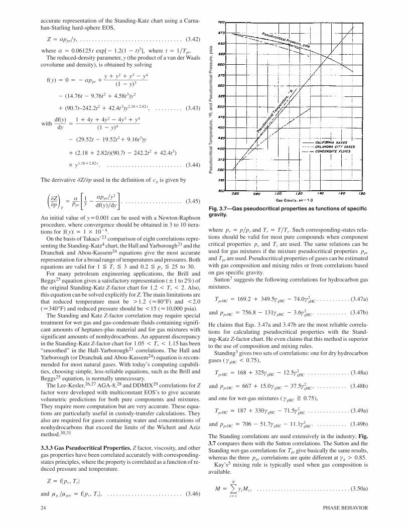
Fig. 3.7—Gas pseudocritical properties as functions of specificgravity.
where pr� p�pc and Tr� T�Tc. Such corresponding-states rela-tions should be valid for most pure compounds when componentcritical properties pc and Tc are used. The same relations can beused for gas mixtures if the mixture pseudocritical properties ppc
and Tpc are used. Pseudocritical properties of gases can be estimatedwith gas composition and mixing rules or from correlations basedon gas specific gravity.
Sutton7 suggests the following correlations for hydrocarbon gasmixtures.
TpcHC� 169.2 � 349.5�gHC� 74.0�2gHC (3.47a). . . . . . . . . . .
and ppcHC� 756.8� 131�gHC � 3.6�2gHC. (3.47b). . . . . . . . . .
He claims that Eqs. 3.47a and 3.47b are the most reliable correla-tions for calculating pseudocritical properties with the Stand-ing-Katz Z-factor chart. He even claims that this method is superiorto the use of composition and mixing rules.
Standing3 gives two sets of correlations: one for dry hydrocarbongases ( �gHC� 0.75),
TpcHC� 168� 325�gHC� 12.5�2gHC (3.48a). . . . . . . . . . . . . .
and ppcHC� 667� 15.0�gHC� 37.5�2gHC, (3.48b). . . . . . . . . .
and one for wet-gas mixtures ( �gHC� 0.75),
TpcHC� 187� 330�gHC� 71.5�2gHC (3.49a). . . . . . . . . . . . . .
and ppcHC� 706� 51.7�gHC� 11.1�2gHC. (3.49b). . . . . . . . . .
The Standing correlations are used extensively in the industry; Fig.3.7 compares them with the Sutton correlations. The Sutton and theStanding wet-gas correlations for Tpc give basically the same results,whereas the three ppc correlations are quite different at �g� 0.85.
Kay’s5 mixing rule is typically used when gas composition isavailable.
M��N
i�1
yi Mi , (3.50a). . . . . . . . . . . . . . . . . . . . . . . . . . . . . . .

GAS AND OIL PROPERTIES AND CORRELATIONS 25
Fig. 3.8—Heptanes-plus (pseudo)critical properties recom-mended for reservoir gases (from Standing,33 after Matthews etal.32).
Tpc��N
i�1
yi Tci , (3.50b). . . . . . . . . . . . . . . . . . . . . . . . . . . . .
and ppc��N
i�1
yi pci , (3.50c). . . . . . . . . . . . . . . . . . . . . . . . . . . .
where the pseudocritical properties of the C7+ fraction can be esti-mated from the Matthews et al.32 correlations (Fig. 3.8),3
Tc C7�� 608 � 364 log�MC7�
� 71.2�
� �2, 450 log MC7�� 3, 800� log �C7�
(3.51a). . . . . .
and pc C7�� 1, 188 � 431 log�MC7�
� 61.1�
� 2, 319� 852 log�MC7�� 53.7����C7�
� 0.8�.
(3.51b). . . . . . . . . . . . . . . . . . .
Kay’s mixing rule is usually adequate for lean natural gases thatcontain no nonhydrocarbons. Sutton suggests that pseudocriticalscalculated with Kay’s mixing rule are adequate up to �g� 0.85, butthat errors in calculated Z factors increase linearly at higher specificgravities, reaching 10 to 15% for �g� 1.5. This bias may be a resultof the C7+ critical-property correlations used by Sutton (not Eqs.3.51a and 3.51b).
When significant quantities of CO2 and H2S nonhydrocarbonsare present, Wichert and Aziz33,31 suggest corrections to arrive atpseudocritical properties that will yield reliable Z factors from theStanding-Katz chart. The Wichert and Aziz corrections are given by
Tpc� T *pc� , (3.52a). . . . . . . . . . . . . . . . . . . . . . . . . . . . . . .
ppc�p*
pc�T *pc� �
T *pc� yH2S�1� yH2S�
, (3.52b). . . . . . . . . . . . . . . . .
and � 120 �yCO2� yH2S�0.9� �yCO2
� yH2S�1.6�
� 15�y0.5H2S� y4
H2S� , (3.52c). . . . . . . . . . . . . . . . . . . . . . .
where T *pc and p*
pc are mixture pseudocriticals based on Kay’s mix-ing rule. This method was developed from extensive data from natu-ral gases containing nonhydrocarbons, with CO2 molar concentra-tion ranging from 0 to 55% and H2S molar concentrations rangingfrom 0 to 74%.
If only gas gravity and nonhydrocarbon content are known, thehydrocarbon specific gravity is first calculated from
�gHC��g��yN2
MN2� yCO2
MCO2�yH2S MH2S��Mair
1� yN2� yCO2
� yH2S.
(3.53). . . . . . . . . . . . . . . . . . . .
Hydrocarbon pseudocriticals are then calculated from Eqs. 3.47aand 3.47b, and these values are adjusted for nonhydrocarbon con-tent on the basis of Kay’s5 mixing rule.
p*pc� �1� yN2
� yCO2� yH2S�ppcHC
� yN2pcN2� yCO2
pc CO2� yH2S pcH2S (3.54a). . . . . . . . . .
and T*pc� (1� yN2
� yCO2� yH2S)TpcHC
� yN2TcN2� yCO2
Tc CO2�yH2STcH2S . (3.54b). . . .
T *c and p*
c are used in the Wichert-Aziz equations with CO2 and H2Smole fractions to obtain mixture Tpc and ppc.
The Sutton7 correlations (Eqs. 3.47a and 3.47b) are recom-mended for hydrocarbon pseudocritical properties. If compositionis available, Kay’s mixing rule should be used with the Matthews etal.32 pseudocriticals for C7+. Gases containing significant amountsof CO2 and H2S nonhydrocarbons should always be corrected withthe Wichert-Aziz equations. Finally, for gas-condensate fluids thewellstream specific gravity, �w (discussed in the next section),should replace �g in the equations above.
3.3.4 Wellstream Specific Gravity. Gas mixtures that produce con-densate at surface conditions may exist as a single-phase gas in thereservoir and production tubing. This can be verified by determin-ing the dewpoint pressure at the prevailing temperature. If well-stream properties are desired at conditions where the mixture issingle-phase, surface-gas and -oil properties must be converted toa wellstream specific gravity, �w. This gravity should be usedinstead of �g to estimate pseudocritical properties.
Wellstream gravityrp represents the average molecular weight ofthe produced mixture (relative to air) and is readily calculated fromthe producing-oil (condensate)/gas ratio, rp; average surface-gasgravity �g ; surface-condensate gravity, �o ; and surface-condensatemolecular weight Mo .
�w��
g� 4, 580 rp �o
1� 133, 000 rp ���M�o, (3.55). . . . . . . . . . . . . . . . . . .
with rp in STB/scf. Average surface-gas gravity is given by
�g�
�Nsp
i�1
Rpi�gi
�Nsp
i�1
Rpi
, (3.56). . . . . . . . . . . . . . . . . . . . . . . . . . . . . .
where Rpi�GOR of Separator Stage i. Standing33 presents Eq.3.55 graphically in Fig. 3.9.
When Mo is not available, Standing gives the following correla-tion.

26 PHASE BEHAVIOR
Fig. 3.9—Wellstream gravity relative to surface average gas grav-ity as a function of solution oil/gas ratio and surface gravities.
Oil/Gas Ratio, STB/MMscf
Mo� 240� 2.22 �API . (3.57). . . . . . . . . . . . . . . . . . . . . . . .
This relation should not be extrapolated outside the range45� �API� 60. Eilerts34 gives a relation for (��M)o ,
���M�o� �1.892� 10�3� � �7.35� 10�5��API
� �4.52� 10�8�� 2API , (3.58). . . . . . . . . . . . . . . . . . .
which should be reliable for most condensates. When condensatemolecular weight is not available, the recommended correlation forMo is the Cragoe35 correlation,
Mo�6, 084
�API � 5.9, (3.59). . . . . . . . . . . . . . . . . . . . . . . . . .
which gives reasonable values for all surface condensates andstock-tank oils.
A typical problem that often arises in the engineering of gas-con-densate reservoirs is that all the data required to calculate well-stream gas volumes and wellstream specific gravity are not avail-able and must be estimated.36-38 In practice, we often report only thefirst-stage-separator GOR (relative to stock-tank-oil volume) andgas specific gravity, Rs1 and �g1, respectively; the stock-tank-oilgravity, �o ; and the primary-separator conditions, psp1 and Tsp1.
To calculate �w from Eq. 3.55 we need total producing OGR, rp,which equals the inverse of Rs1 plus the additional gas that will bereleased from the first-stage separator oil, Rs�,
rp�1
�Rs1 � Rs��. (3.60). . . . . . . . . . . . . . . . . . . . . . . . . . .
Rs� can be estimated from several correlations.37,39 Whitson38 pro-poses use of a bubblepoint pressure correlation (e.g., the Standing40
correlation),
Rs� � A1�g� (3.61a). . . . . . . . . . . . . . . . . . . . . . . . . . . . . . . . .
and A1� � psp1
18.2� 1.4�10�0.0125�API�0.00091Tsp1
��1.205
,
(3.61b). . . . . . . . . . . . . . . . . . .
with psp1 in psia, Tsp1 in °F, and Rs� in scf/STB. �g� is the gas grav-ity of the additional solution gas released from the separator oil. TheKatz41 correlation (Fig. 3.10) can be used to estimate �g�, where abest-fit representation of his graphical correlation is
�g� � A2� A3 Rs�, (3.62). . . . . . . . . . . . . . . . . . . . . . . . . .
where A2� 0.25� 0.02�API and A3�� (3.57� 10�6)�API .
Fig. 3.10—Correlation for separator-oil dissolved gas gravity asa function of stock-tank-oil gravity and separator-oil GOR (fromRef. 41).
Solution Gas/Oil Ratio, scf/STB
Solving Eqs. 3.61 and 3.62 for Rs� gives
Rs� �A1 A2
�1� A1 A3�
. (3.63). . . . . . . . . . . . . . . . . . . . . . . . . .
Average surface separator gas gravity, �g, is given by
�g�
�g1 Rs1� �g� Rs�
Rs1� Rs�. (3.64). . . . . . . . . . . . . . . . . . . . . .
Although the Katz correlation is only approximate, the impact of afew percent error in �g� is not of practical consequence to the cal-culation of �w because Rs� is usually much less than Rs1.
3.3.5 Gas Viscosity. Viscosity of reservoir gases generally rangesfrom 0.01 to 0.03 cp at standard and reservoir conditions, reachingup to 0.1 cp for near-critical gas condensates. Estimation of gas vis-cosities at elevated pressure and temperature is typically a two-stepprocedure: (1) calculating mixture low-pressure viscosity �gsc atpsc and T from Chapman-Enskog theory3,6 and (2) correcting thisvalue for the effect of pressure and temperature with a correspond-ing-states or dense-gas correlation. These correlations relate the ac-tual viscosity �g at p and T to low-pressure viscosity by use of theratio �g��gsc or difference ( �g� �gsc) as a function of pseudore-duced properties ppr and Tpr or as a function of pseudoreduced den-sity �pr.
Gas viscosities are rarely measured because most laboratories donot have the required equipment; thus, the prediction of gas viscos-ity is particularly important. Gas viscosity of reservoir systems isoften estimated from the graphical correlation �g��gsc� f(Tr, pr)proposed by Carr et al.42 (Fig. 3.11). Dempsey43 gives a polynomialapproximation of the Carr et al. correlation. With these correlations,gas viscosities can be estimated with an accuracy of about �3% formost applications. The Dempsey correlation is valid in the range1.2� Tr� 3 and 1� pr� 20.
The Lee-Gonzalez gas viscosity correlation (used by most PVTlaboratories when reporting gas viscosities) is given by44
�g� A1� 10�4 exp�A2�A3g� , (3.65a). . . . . . . . . . . . . . . . . .
where A1��9.379� 0.01607Mg�T1.5
209.2� 19.26Mg� T,
A2� 3.448� �986.4�T� � 0.01009Mg ,
and A3� 2.447� 0.2224A2 , (3.65b). . . . . . . . . . . . . . . . . . . .
with �g in cp, �g in g/cm3, and T in °R. McCain19 indicates the ac-curacy of this correlation is 2 to 4% for �g�1.0, with errors up to20% for rich gas condensates with �g� 1.5.

GAS AND OIL PROPERTIES AND CORRELATIONS 27
Fig. 3.11—Carr et al.42 gas-viscosity correlation.
Pseudoreduced Temperature, Tr
Molecular Weight
Gas Gravity (air�1)
H2S, mol%
N2, mol% CO2, mol%
go
Lucas45 proposes the following gas viscosity correlation, whichis valid in the range 1� Tr� 40 and 0� pr� 100 (Fig. 3.12)6:
�g��gsc� 1 �A1 p1.3088
pr
A2 pA5pr � �1 � A3 pA4
pr��1
, (3.66a). . . . . . .
where A1�(1.245� 10�3) exp�5.1726T�0.3286
pr�
Tpr,
A2� A1�1.6553Tpr� 1.2723� ,
A3�0.4489 exp�3.0578T�37.7332
pr�
Tpr,
A4�1.7368 exp�2.2310T�7.6351
pr�
Tpr,
and A5� 0.9425 exp�� 0.1853T 0.4489pr� , (3.66b). . . . . . . . . . .
where �gsc�� 0.807T 0.618pr � 0.357 exp�� 0.449Tpr�
� 0.340 exp�� 4.058Tpr� � 0.018� ,
�� 9, 490� Tpc
M3p4pc�
1�6
,
and ppc� RTpc
�N
i�1
yi Zci
�N
i�1
yivci
, (3.67). . . . . . . . . . . . . . . . . . . . . . . .
with � in cp�1, T and Tc in °R, and pc in psia. Special correctionsshould be applied to the Lucas correlation when polar compounds,such as H2S and water, are present in a gas mixture. The effect ofH2S is always �1% and can be neglected, and appropriate correc-tions can be made to treat water if necessary.
Given its wide range of applicability, the Lucas method is recom-mended for general use. When compositions are not available, cor-relations for pseudocritical properties in terms of specific gravitycan be used instead. Standing2 gives equations for �gsc in terms of�g, temperature, and nonhydrocarbon content,
�gsc� ��gsc�uncorrected� ��N2
� ��CO2� ��H2S ,
(3.68a). . . . . . . . . . . . . . . . . . . .

28 PHASE BEHAVIOR
Fig. 3.12—Lucas45 corresponding-states generalized viscositycorrelation (Ref. 6); ��dynamic viscosity and �p�micro-poise�10�6 poise�10�4 cp.
������� � ���� � � �� ��
���������������
� � �� �� �� �� �� ����
��������
where ��gsc�uncorrected� �8.188� 10�3� � �1.709� 10�5�
� �2.062� 10�6��g�T� �6.15� 10�3� log �g ,
��N2� yN2
�8.48� 10�3� log �g� �9.59� 10�3��,
��CO2� yCO2
�9.08� 10�3� log �g� �6.24� 10�3��,
and ��H2S� yH2S �8.49� 10�3� log �g� �3.73� 10�3��.
(3.68b). . . . . . . . . . . . . . . . . . .
Reid et al.6 review other gas viscosity correlations with accuracysimilar to that of the Lucas correlation.
3.3.6 Dewpoint Pressure. The prediction of retrograde dewpointpressure is not widely practiced. It is generally recognized that thecomplexity of retrograde phase behavior necessitates experimentaldetermination of the dewpoint condition. Sage and Olds’46 data areperhaps the most extensive tabular correlation of dewpoint pressur-es. Eilerts et al.47,48 also present dewpoint pressures for severallight-condensate systems.
Nemeth and Kennedy49 have proposed a dewpoint correlationbased on composition and C7+ properties.
ln pd�A1 zC2� zCO2
� zH2S�zC6�2(zC3
�zC4)� zC5
� 0.4zC1�0.2zN2� � A2�C7�
� A3���
zC1
�zC7�� 0.002����
� A4T��A5zC7�MC7��� A6�zC7�
MC7��2
� A7�zC7�MC7�� 3� A8���
MC7�
��C7�� 0.0001��
��
� A9���
MC7�
� �C7�� 0.0001��
��
2
� A10���
MC7�
��C7�� 0.0001��
��
3
� A11 , (3.69). . . . . . . . . . . . . . . . . . . . . . . . . . . . . . . . . .
where A1��2.0623054, A2�6.6259728, A3��4.4670559�10�3, A4�1.0448346�10�4, A5�3.2673714�10�2, A6��3.6453277�10�3, A7�7.4299951�10�5, A8��1.1381195�10�1, A9�6.2476497�10�4, A10��1.0716866�10�6, andA11�1.0746622�101.
The range of properties used to develop this correlation includesdewpoints from 1,000 to 10,000 psia, temperatures from 40 to 320°F,and a wide range of reservoir compositions. The correlation usuallycan be expected to predict dewpoints with an accuracy of �10% forcondensates that do not contain large amounts of nonhydrocarbons.This is acceptable in light of the fact that experimental dewpoint pres-sures are probably determined with an accuracy of only �5%. Thecorrelation is generally used only for preliminary reservoir studiesconducted before an experimental dewpoint is available.
Organick and Golding50 and Kurata and Katz51 present graphicalcorrelations for dewpoint pressure.
3.3.7 Total FVF. Total FVF,3,17,46 Bt, is defined as the volume ofa two-phase, gas-oil mixture (or sometimes a single-phase mixture)at elevated pressure and temperature divided by the stock-tank-oilvolume resulting when the two-phase mixture is brought to surfaceconditions,
Bt�Vo� Vg
(Vo)sc�
Vo� Vg
Vo. (3.70). . . . . . . . . . . . . . . . . . . . .
Bt is used for calculating the oil in place for gas-condensate reser-voirs, where Vo� 0 in Eq. 3.70. Assuming 1 res bbl of hydrocar-bon PV, the initial condensate in place is given by N� 1�Bt (inSTB) and the initial “dry” separator gas in place is G� N�rp,where rp�initial producing (solution) OGR.
For gas-condensate systems, Sage and Olds46 give a tabulatedcorrelation for Bt.
Bt�RpT
p Z*, (3.71). . . . . . . . . . . . . . . . . . . . . . . . . . . . . . . .
where Rp�producing GOR in scf/STB, Bt is in bbl/STB, T is in °R,and p is in psia. Z* varies with pressure and temperature, where thetabulated correlation for Z* is well represented by
Z*� A0� A1p� A2p1.5� A3
pT� A4
p1.5
T, (3.72). . . . . . . .
where A0�5.050�10�3, A1��2.740�10�6, A2�3.331�10�8,A3�2.198�10�3, and A4��2.675�10�5 with p in psia and Tin °R. Although the Sage and Olds data only cover the range600�p�3,000 psia and 100�T�250°F, Eq. 3.72 gives acceptableresults up to 10,000 psia and 350°F (when gas volume is much largerthan oil volume).
When reservoir hydrocarbon volume consists only of gas, the fol-lowing relations apply for total FVF.
Bt� Bgd Rp� Bgw �Rp� Cog� , (3.73a). . . . . . . . . . . . . . . . .
Cog� 133, 000 ��o�Mo
� , (3.73b). . . . . . . . . . . . . . . . . . . . . .
Mo� 6, 084���API� 5.9� , (3.73c). . . . . . . . . . . . . . . . . . . . .
and �API� 141.5�(131.5� �o) , (3.73d). . . . . . . . . . . . . . . . .
where Bgd�dry gas FVF in ft3/scf, Bgw�wet-gas FVF in ft3/scf(given by Eq. 3.38), Cog�gas equivalent conversion factor in scf/STB (see Chap. 7), and Rp�producing GOR in scf/STB.

GAS AND OIL PROPERTIES AND CORRELATIONS 29
Fig. 3.13—Effect of paraffinicity, Kw, on bubblepoint pressure.
C7+ Watson Characterization Factor, KwC7+ C7+ Watson Characterization Factor, KwC7+
PR EOSGlasø UncorrectedGlasø Corrected
Standing3 gives a graphical correlation for Bt using a correlationparameter A defined as
A� RpT 0.5
�0.3g
�ao , (3.74). . . . . . . . . . . . . . . . . . . . . . . . . . . . . . .
where a� 2.9� 10�0.00027 Rp. Standing’s correlation is valid forboth oil and gas-condensate systems and can be represented with
log Bt�� 5.262� 47.4� 12.22� log A* , (3.75a). . . . . . . . .
where log A*� log A��10.1� 96.86.604� log p
� (3.75b). .
and A is given by Eq. 3.74. On the basis of data from North Sea oils,Glasø52 gives a correlation for Bt using the Standing correlation pa-rameter A (Eq. 3.74):
log Bt� �8.0135� 10�2� � 0.47257 log A*
� 0.17351�log A* �2 , (3.76). . . . . . . . . . . . . . . . . . . . .
where A*�Ap�1.1089.Either the Standing or the Glasø correlations for Bt can be used
with approximately the same accuracy. However, neither correla-tion is consistent with the limiting conditions
Bt� Bo for Vg� 0 (3.77a). . . . . . . . . . . . . . . . . . . . . . . . . .
and Bt� Bgd Rp for Vo� 0. (3.77b). . . . . . . . . . . . . . . . . . .
Bt correlations evaluated at a bubblepoint usually will underpredictthe actual Bob by �0.2.
��" �� �!����
This section gives correlations for PVT properties of reservoir oils,including bubblepoint pressure and oil density, compressibility,FVF, and viscosity. With only a few exceptions, oil properties havebeen correlated in terms of surface-oil and -gas properties, includingsolution gas/oil ratio, oil gravity, average surface-gas gravity, andtemperature. A few correlations are also given in terms of composi-tion and component properties.
Reservoir oils typically contain dissolved gas consisting mainlyof methane and ethane, some intermediates (C3 through C6), andlesser quantities of nonhydrocarbons. The amount of dissolved gashas an important effect on oil properties. At the bubblepoint a dis-continuity in the system volumetric behavior is caused by gas com-ing out of solution, with the system compressibility changing dra-
matically.8 An accurate method is needed to correlate thebubblepoint pressure, temperature, and solution gas/oil ratio.
Oil properties can be grouped into two categories: saturated andundersaturated properties. Saturated properties apply at pressures ator below the bubblepoint, and undersaturated properties apply atpressures greater than the bubblepoint. For oils with initial GOR’sless than �500 scf/STB, assuming linear variation of undersaturat-ed-oil properties with pressure is usually acceptable.
3.4.1 Bubblepoint Pressure. The correlation of bubblepoint pres-sure has received more attention than any other oil-property correla-tion. Standing3,17,40 developed the first accurate bubblepoint cor-relation, which was based on California crude oils.
pb� 18.2�A� 1.4�, (3.78). . . . . . . . . . . . . . . . . . . . . . . . . .
where A� �Rs��g�0.83 10�0.00091T�0.0125�API�, with Rs in scf/STB, T
in °F, and pb in psia.Lasater53 used a somewhat different approach to correlate bub-
blepoint pressure, where mole fraction yg of solution gas in the res-ervoir oil is used as the main correlating parameter17:
pb� A T�g
, (3.79). . . . . . . . . . . . . . . . . . . . . . . . . . . . . . . . . .
with T in °R and pb in psia. The function A(yg) is given graphicallyby Lasater, and his correlation can be accurately described by
A� 0.83918� 101.17664yg y0.57246g ; yg� 0.6 (3.80a). . . . . . . .
and A� 0.83918� 101.08000yg y0.31109g ; yg� 0.6, (3.80b). . . . .
where yg� 1 � 133, 000 ���M�oRs��1
, (3.81). . . . . . . . . . . .
with Rs in scf/STB. In this correlation, the gas mole fraction is de-pendent mainly on solution gas/oil ratio, but also on the propertiesof the stock-tank oil. The Cragoe35 correlation given by Eq. 3.59 isrecommended for estimating Mo when stock-tank-oil molecularweight is not known.
Standing’s approach was used by Glasø52 for North Sea oils, re-sulting in the correlation
log pb� 1.7669� 1.7447 log A� 0.30218(log A)2,
(3.82). . . . . . . . . . . . . . . . . . . .
where A� �Rs��g�0.816 �T 0.172��0.989API� with pb in psia, T in °F and
Rs in scf/STB. Glasø’s corrections for nonhydrocarbon contentand stock-tank-oil paraffinicity are not widely used, primarily be-

30 PHASE BEHAVIOR
cause the necessary data are not available. Sutton and Farshad54
mention that the API correction for paraffinicity worsened bubble-point predictions for gulf coast fluids. Fig. 3.13 gives an explana-tion for this observation.
Fig. 3.13 shows the effect of paraffinicity (which is quantified bythe Watson characterization factor, Kw) on bubblepoint pressure;the figure is based on calculations with a tuned EOS for an Asian oil(solid circles). The oil composition is constant in the example cal-culation. The 12 C7+ fractions are each split into a paraffinic pseudo-component and an aromatic pseudocomponent (i.e., 24 C7+ pseudo-components). The paraffinic fraction was varied, and bubblepointcalculations were made. The variation in paraffinicity is expressedin terms of the overall C7+ Watson characterization factor. Alsoshown in the figure are the variation in solution gas/oil ratio and theoil specific gravity with KwC7�
.The actual reservoir oil has a KwC7�
� 11.55, where the EOSbubblepoint is close to the uncorrected Glasø bubblepoint predic-tion. When the correction for paraffinicity is applied, the correctiongives a poorer bubblepoint prediction (even though the overall trendin bubblepoints is improved by the Glasø paraffinicity corrections).
A quantitatively similar correction to the Glasø correction (buteasier to use) is based on the estimate for Whitson’s55,56 Watsoncharacterization factor, Kw, and yields
��o� corrected� ��o�measured�Kw�11.9�1.1824. (3.83). . . . . . . . . . .
The corrected specific gravity correlation is used in the Glasø bubble-point correlation instead of the measured specific gravity. An estimateof Kw for the stock-tank oil must be available to use this correction.
Vazquez and Beggs57 give the following correlations. For�API� 30,
pb����
27.64�Rs�gc�10��11.172 �API
T�460����
0.9143
, (3.84). . . . . . . . . .
and, for �API� 30,
pb� 56.06�Rs�gc� 10��10.393�API
T�460��
0.8425
, (3.85). . . . . . . . .
with pb in psia, T in °F and Rs in scf/STB. These equations are basedon a large number of data from commercial laboratories. Vazquezand Beggs correct for the effect of separator conditions using a mo-dified gas specific gravity, �gc, which is correlated with first-stage-separator pressure and temperature, and stock-tank-oil gravity.
�gc� �g 1� �0.5912� 10�4� �APITsp log� psp
114.7��,
(3.86). . . . . . . . . . . . . . . . . . . .
with Tsp in °F and psp in psia.Standing’s correlation can be used to develop field- or reservoir-
specific bubblepoint correlations. A linear relation is usually as-sumed between bubblepoint pressure and the Standing correlatingcoefficient. This is a standard approach used in the industry, and theStanding bubblepoint correlating parameter is well suited for devel-oping field-specific correlations.
Sometimes the solution gas/oil ratio is needed at a given pressure,and this is readily calculated by solving the bubblepoint correlationfor Rs. For the Standing correlation,
Rs� �g (0.055p� 1.4)100.0125�API
100.00091T�
1.205
; (3.87). . . . . . . . .
similar relations can be derived for the other bubblepoint correlations.
In summary, significant differences in predicted bubblepoint pres-sures should not be expected for most reservoir oils with most of theprevious correlations. The Lasater and Standing equations are recom-mended for general use and as a starting point for developing reser-voir-specific correlations. Correlations developed for a specific re-gion, such as Glasø’s correlation for the North Sea, should probablybe used in that region and, in the case of Glasø’s correlation, may beextended to other regions by use of the paraffinicity correction.
3.4.2 Oil Density. Density of reservoir oil varies from 30 lbm/ft3 forlight volatile oils to 60 lbm/ft3 for heavy crudes with little or no solu-tion gas. Oil compressibility may range from 3�10�6 psi�1 forheavy crude oils to 50�10�6 psi�1 for light oils. The variation ofoil compressibility with pressure is usually small, although for vola-tile oils the effect can be significant, particularly for material-balanceand reservoir-simulation calculations of highly undersaturated vola-tile oils. Several methods have been used successfully to correlate oilvolumetric properties, including extensions of ideal-solution mixing,EOS’s, corresponding-states correlations, and empirical correlations.
Oil density based on black-oil properties is given by
�o�62.4�o� 0.0136�g Rs
Bo, (3.88). . . . . . . . . . . . . . . . . . . .
with �o in lbm/ft3, Bo in bbl/STB, and Rs in scf/STB. Correlationscan be used to estimate Rs and Bo from �o, �g, p, and T.
Standing-Katz Method. Standing3,17 and Standing and Katz58
give an accurate method for estimating oil densities that uses an ex-tension of ideal-solution mixing.
�o� �po� ��p� ��T , (3.89). . . . . . . . . . . . . . . . . . . . . .
where �po is the pseudoliquid density at standard conditions and theterms ��T and ��p give corrections for temperature and pressure,respectively. Pseudoliquid density is calculated with ideal-solutionmixing and correlations for the apparent liquid densities of ethane
Fig. 3.14—Apparent liquid densities of methane and ethane(from Standing33).
System Density at 60°F and 14.7 psia, g/cm3

GAS AND OIL PROPERTIES AND CORRELATIONS 31
Fig. 3.15—Chart for calculating pseudoliquid density of reservoir oil (from Standing33).
g
and methane at standard conditions. Given oil composition xi, �po
is calculated from
�po�
�N
i�1
xi Mi
�N
i�1
�xi Mi��i�
, (3.90). . . . . . . . . . . . . . . . . . . . . . . . . . .
where Standing and Katz show that apparent liquid densities �i ofC2 and C1 are functions of the densities �2� and �po, respectively(Fig. 3.14).
�C2� 15.3� 0.3167 �C2�
�C1� 0.312� 0.45 �po , (3.91). . . . . . . . . . . . . . . . . . . . . . .
where �C2��
�C7�
i�C2
xi Mi
�C7�
i�C2
�xi Mi��i�
, (3.92). . . . . . . . . . . . . . . . . . . .
with � in lbm/ft3. Application of these correlations results in an ap-parent trial-and-error calculation for �po. Standing33 presents agraphical correlation (Fig. 3.15) based on these relations, where �po
is found from �C3� and weight fractions of C2 and C1 (wC2
and wC1,
respectively).Figs. 3.16 and 3.17 show the pressure and temperature correc-
tions, ��p and ��T
, graphically. ��p is a function of �po, and ��T
is a function of ( �po� ��p). Madrazo59 introduced modifiedcurves for ��p and ��
T that improve predictions at higher pressur-
es and temperatures. Standing3 gives best-fit equations for his origi-nal graphical correlations of ��p and ��
T (Eqs. 3.98 and 3.99),
which are not recommended at temperatures �240°F; instead, Ma-drazo’s graphical correlation can be used. The correction factors canalso be used to determine isothermal compressibility and oil FVF atundersaturated conditions.
The treatment of nonhydrocarbons in the Standing-Katz methodhas not received much attention, and the method is not recom-mended when concentrations of nonhydrocarbons exceed 10 mol%.Standing3 suggests that an apparent liquid density of 29.9 lbm/ft3
can be used for nitrogen but does not address how the nonhydrocar-bons should be considered in the calculation procedure (i.e., as partof the C3+ material or following the calculation of �C2
and �C1).
Madrazo indicates that the volume contribution of nonhydrocar-

32 PHASE BEHAVIOR
Fig. 3.16—Pressure correction to the pseudoliquid density at 14.7 psia and 60°F (from Ref. 59).
Density of System at 60°F and 14.7 psia, lbm/ft3
bons can be neglected completely if the total content is �6 mol%.Vogel and Yarborough60 suggest that the weight fraction of nitrogenshould be added to the weight fraction of ethane.
Using additive volumes and Eqs. 3.91 and 3.92, we can show that�C2�
and �po can be calculated explicitly. Thus, the following is themost direct procedure for calculating �o from the Standing-Katzmethod.
1. Calculate the mass of each component.
mi� xi Mi . (3.93). . . . . . . . . . . . . . . . . . . . . . . . . . . . . . . . . .
2. Calculate VC3�.
VC3�� �
C7�
i�C3
mi�i
, (3.94). . . . . . . . . . . . . . . . . . . . . . . . . . . . . .
where �i are component densities at standard conditions (Appen-dix A).
3. Calculate �C2�.
�C2��� b� b2� 4ac�
2a, (3.95). . . . . . . . . . . . . . . . . . . .
where a� 0.3167VC3�, b� mC2
�0.3167mC2�� 15.3VC3�
,and c�� 15.3mC2�
.4. Calculate VC2�
.
VC2�� VC3�
�mC2�C2
� VC3��
mC2
15.3� 0.3167�C2�
. (3.96). . . . . . . . . . . .
5. Calculate �po.
�po��b � b2 � 4ac�
2a, (3.97). . . . . . . . . . . . . . . . . . . . .
where a� 0.45VC2�, b� mC1
� 0.45mC1�� 0.312VC2�
, andc�� 0.312mC1�
.6. Calculate the pressure effect on density.
��p� 10�3 0.167� �16.181� 10�0.0425�po�� p
� 10�8 0.299� �263� 10�0.0603�po�� p2. (3.98). . . . .

GAS AND OIL PROPERTIES AND CORRELATIONS 33
Fig. 3.17—Temperature correction to the pseudoliquid density at pressure and 60°F (from Ref. 59).
Density of System at Pressure and 60°F, lbm/ft3
7. Calculate the temperature effect on density.
��T� (T� 60) 0.0133� 152.4��po� ��p��2.45�
� (T� 60)2��8.1� 10�6�
� 0.0622� 10�0.0764(�po�� �p)�� . (3.99). . . . . . . . . . .
8. Calculate mixture density from Eq. 3.89.In the absence of oil composition, Katz41 suggests calculating the
pseudoliquid density from stock-tank-oil gravity, �o, solution gas/oil ratio, Rs, and apparent liquid density of the surface gas, �ga, tak-en from a graphical correlation (Fig. 3.18),
�po�62.4�o� 0.0136 Rs �g
1� 0.0136�Rs �g��ga�. (3.100). . . . . . . . . . . . . . . . . .
Standing gives an equation for �ga.
�ga� 38.52� 10�0.00326 �API
� (94.75� 33.93 log �API) log �g , (3.101). . . . . . . . . . .
with �ga in lbm/ft3 and Rs in scf/STB.Alani-Kennedy61 Method. The Alani-Kennedy method for cal-
culating oil density is a modification of the original van der WaalsEOS, with constants a and b given as functions of temperature fornormal paraffins C1 to C10 and iso-butane (Table 3.1); two sets ofcoefficients are reported for methane (for temperatures from 70 to300°F and from 301 to 460°F) and two sets for ethane (for tempera-tures from 100 to 249°F and from 250 to 460°F). Lohrenz et al.62
give Alani-Kennedy temperature-dependent coefficients for non-hydrocarbons N2, CO2, and H2S (Table 3.1). The Alani-Kennedyequations are summarized next. Eqs. 3.102b and 3.102c are in theoriginal van der Waals EOS but are not used.
p� RTv� b
� av2 , (3.102a). . . . . . . . . . . . . . . . . . . . . . . . . . . .

34 PHASE BEHAVIOR
Fig. 3.18—Apparent pseudoliquid density of separator gas (fromStanding,33 after Katz41).
ai �2764
R2T 2ci
pci, (3.102b). . . . . . . . . . . . . . . . . . . . . . . . . . . .
bi �18
RTcipci
, (3.102c). . . . . . . . . . . . . . . . . . . . . . . . . . . . . .
a��N
i�1
xi ai , (3.102d). . . . . . . . . . . . . . . . . . . . . . . . . . . . . .
b��N
i�1
xi bi , (3.102e). . . . . . . . . . . . . . . . . . . . . . . . . . . . . . .
ai�a1i
T� log a2i; i� C7�, (3.102f). . . . . . . . . . . . . . . . . .
and bi� b1iT� b2i ; i� C7�, (3.102g). . . . . . . . . . . . . . . . .
where log aC7�� �3.8405985� 10�3�MC7�
� �9.5638281� 10�4�MC7��C7�
� 261.80818T
� �7.3104464� 10�6�M2C7�
� 10.753517 (3.103a). . . . . . . . . . . . . . . . . . . . .
and bC7�� �3.499274� 10�2�MC7�
� 7.2725403�C7�
� �2.232395� 10�4�T� �1.6322572� 10�2�MC7��C7�
� 6.2256545, (3.103b). . . . . . . . . . . . . . . . . . . . . . .
with � in lbm/ft3, v in ft3/lbm mol, T in °R, p in psia, and R�univer-sal gas constant�10.73.
Solution of the cubic equation for volume is presented in Chap.4. Density is given by ��M/v, where M is the mixture molecularweight and v is the molar volume given by the solution to the cubicequation. The Alani-Kennedy method can also be used to estimateoil compressibilities.
Rackett,63 Hankinson and Thomson,64 and Hankinson et al.65
give accurate correlations for pure-component saturated-liquid den-sities, and although these correlations can be extended to mixtures,they have not been tested extensively for reservoir systems. Cullicket al.66 give a modified corresponding-states method for predictingdensity of reservoir fluids, The method has a better foundation andextrapolating capability than the methods discussed previously(particularly for systems with nonhydrocarbons); however, spacedoes not allow presentation of the method in its entirety.
Either the Standing-Katz or Alani-Kennedy method should esti-mate the densities of most reservoir oils with an accuracy of �2%.The Alani-Kennedy method is suggested for systems at tempera-tures �250°F and for systems containing appreciable amounts ofnonhydrocarbons (�5 mol%). Cubic EOS’s (e.g., Peng-Robinsonor Soave-Redlich-Kwong) that use volume translation also estimateliquid densities with an accuracy of a few percent (e.g., the recom-mended characterization procedures in Chap. 5 or other proposedcharacterizations67,68).
TABLE 3.1—CONSTANTS FOR ALANI-KENNEDY61 OIL DENSITY CORRELATION
Component a1 a2 b1�104 b2
N2 4,300 2.293 4.49 0.3853
CO2 8,166 126.0 0.1818 0.3872
H2S 13,200 0.0 17.9 0.3945
C1
At 70 to 300°F 9,160.6413 61.893223 �3.3162472 0.50874303
At 300 to 460°F 147.47333 3,247.4533 �14.072637 1.8326695
C2
At 100 to 250°F 46,709.573 �404.48844 5.1520981 0.52239654
At 250 to 460°F 17,495.343 34.163551 2.8201736 0.62309877
C3 20,247.757 190.24420 2.1586448 0.90832519
i-C4 32,204.420 131.63171 3.3862284 1.1013834
n-C4 33,016.212 146.15445 2.902157 1.1168144
i-C5 37,046.234 299.62630 2.1954785 1.4364289
n-C5 37,046.234 299.62630 2.1954785 1.4364289
n-C6 52,093.006 254.56097 3.6961858 1.5929406
n-C7 82,295.457 64.380112 5.2577968 1.7299902
n-C8 89,185.432 149.39026 5.9897530 1.9310993
n-C9 124,062.650 37.917238 6.7299934 2.1519973
n-C10 146,643.830 26.524103 7.8561789 2.3329874

GAS AND OIL PROPERTIES AND CORRELATIONS 35
3.4.3 Undersaturated-Oil Compressibility. With measured dataor an appropriate correlation for Bo or �o, Eq. 3.14 readily definesthe isothermal compressibility of an oil at pressures greater than thebubblepoint. “Instantaneous” undersaturated-oil compressibility,defined by Eq. 3.15 with the pressure derivative evaluated at a spe-cific pressure, is used in reservoir simulation and well-test inter-pretation. Another definition of oil compressibility may be used inmaterial-balance calculations (e.g., Craft and Hawkins69)—the“cumulative” or “average” compressibility defines the cumulativevolumetric change of oil from the initial reservoir pressure to cur-rent reservoir pressure.
co� p� �
Voi�pi
p
co� p� dp
Voi�pi� p�
� � � 1Voi� Voi� Vo�p�
pi� p �. (3.104). . . . . . . . . . . . . . . .
The cumulative compressibility is readily identified because it ismultiplied by the cumulative reservoir pressure drop, pi� pR. Usu-ally co is assumed constant; however, this assumption may not bejustified for high-pressure volatile oils.
Oil compressibility is used to calculate the variation in undersatu-rated density and FVF with pressure.
�o� �ob exp co�p� pb��
� �ob 1� co�pb� p�� (3.105a). . . . . . . . . . . . . . . . . . . . .
and Bo� Bob exp co�pb� p��
�Bob 1� co�p� pb
�� , (3.105b). . . . . . . . . . . . . . . . .
where consistent units must be used. These equations are derivedfrom the definition of isothermal compressibility assuming that co isconstant. When oil compressibility varies significantly with pressure,Eqs. 3.105a and 3.105b are not really valid. The approximations�o� �ob [1� co( pb� p)] and Bo�Bob [1� co( p� pb)] areused in many applications, and to predict volumetric behavior cor-rectly with these relations requires that co be defined by
co(p)��� 1Vob� Vo�p� � Vob
p� pb� . (3.106). . . . . . . . . . . . . . .
Strictly speaking, the compressibility of an oil mixture is definedonly for pressures greater than the bubblepoint pressure. If an oil isat its bubblepoint, the compressibility can be determined and de-fined only for a positive change in pressure. A reduction in pressurefrom the bubblepoint results in gas coming out of solution and, sub-sequently, a change in the mass of the original system for whichcompressibility is to be determined. Implicit in the definition ofcompressibility is that the system mass remains constant.
Vazquez and Beggs57 propose the following correlation forinstantaneous undersaturated-oil compressibility.
co� A�p, (3.107). . . . . . . . . . . . . . . . . . . . . . . . . . . . . . . . . .
whereA� 10�5(5Rsb� 17.2T� 1, 180�gc� 12.61�API� 1, 433), withco in psi�1, Rsb in scf/STB, T in °F, and p in psia. With this correla-tion for oil compressibility, undersaturated-oil FVF can be calcu-lated analytically from
Bo� Bob( pb�p) A. (3.108). . . . . . . . . . . . . . . . . . . . . . . . . . .
If measured pressure/volume data are available (see Sec. 6.4 inChap. 6), these data can be used to determine A (e.g., by plottingVo�Vob vs. p�pb on log-log paper). Constant A can then be used tocompute compressibilities from the simple relation co� A�p.
Fig. 3.19—Undersaturated-oil-compressibility correlation (fromStanding33).
Bubblepoint Oil Density, lbm/ft3
Compressibility atBubblepoint +
BubblepointPlus 1,000 psia
BubblepointPlus 2,000 psia
Constant A determined in this way is a useful correlating parameter,one that helps to identify erroneous undersaturated p-Vo data.
Standing33 gives a graphical correlation for undersaturated co
(Fig. 3.19) that can be represented by
co� 10�6 exp �ob� 0.004347 �p� pb� � 79.1
(7.141� 10�4)�p� pb� � 12.938�,
(3.109). . . . . . . . . . . . . . . . . . .
with co in psi�1, �ob in lbm/ft3, and p in psia.The Alani-Kennedy EOS can also be solved analytically for oil
compressibility, and Trube70 gives a corresponding-states methodfor determining oil compressibility with charts.
Any of the correlations mentioned here should yield reasonableestimates of co. However, we recommend that experimental data beused for volatile oils when co is greater than about 20�10�6 psi�1.A simple polynomial fit of the relative volume data, Vro� Vo�Vob,from a PVT report allows an accurate and explicit equation for un-dersaturated-oil compressibility.
Vro� A0� A1 p� A2 p2 (3.110a). . . . . . . . . . . . . . . . . . . . . . .
and co��1
Vro�Vro
p�
T
�� �A1� 2A2 p�
A0� A1 p� A2 p2 , (3.110b). . . . . . . . . . . . . . . . . . . .
where A0, A1, and A2 are determined from experimental data. Alter-natively, measured data can be fit by use of Eq. 3.108.
3.4.4 Bubblepoint-Oil FVF. Oil FVF ranges from 1 bbl/STB foroils containing little solution gas to about 2.5 bbl/STB for volatileoils. Bob increases more or less linearly with the amount of gas insolution, a fact which explains why Bob correlations are similar tobubblepoint pressure correlations. For example, Standing’s3,17,40
correlation for California crude oils is
Bob� 0.9759� �12� 10�5�A1.2, (3.111). . . . . . . . . . . . . . .
where A� Rs��g��o� 0.5� 1.25T.

36 PHASE BEHAVIOR
Glasø’s52 correlation for North Sea crude oils is
log�Bob� 1� � � 6.585� 2.9133 log A� 0.2768�log A�2 ,
(3.112). . . . . . . . . . . . . . . . . . . .
where A� Rs ��g��o� 0.526� 0.968T.The Vazquez and Beggs57 correlation, based on data from com-
mercial laboratories, is
Bob� 1� �4.677� 10�4�Rs� �0.1751� 10�4�(T� 60)
���API�gc�� �1.8106� 10�8�Rs(T� 60)��API
�gc�
(3.113a). . . . . . . . . . . . . . . . . .
for �API� 30 and
Bob� 1� �4.67� 10�4�Rs� �0.11� 10�4�(T� 60)��API�gc�
� �0.1337� 10�8�Rs(T� 60)��API�gc� (3.113b). . . . . . . . .
for �API� 30, where the effect of separator conditions is includedby use of a corrected gas gravity �gc (Eq. 3.86).
The Standing and the Vazquez-Beggs correlations indicate that aplot of Bo vs. Rs should correlate almost linearly. This plot is usefulfor checking the consistency of reported PVT data from a differen-tial liberation plot. Eq. 3.114,71 which performs considerably betterfor Middle Eastern oils, also suggests a linear relationship betweenBob and Rs.
Bob� 1.0� �0.177342� 10�3� Rs� �0.220163� 10�3�
� Rs��g��o� ��4.292580� 10�6�Rs(T� 60)(1� �o)
��0.528707� 10�3�(T� 60). (3.114). . . . . . . . . . . . . . .
All three Bob correlations (Eqs. 3.113a, 3.113b, and 3.114)should give approximately the same accuracy. Sutton and Far-shad’s54 comparative study of gulf coast oils indicates that Stand-ing’s correlation is slightly better for Bob� 1.4 and that Glasø’scorrelation is best for Bob� 1.4.
3.4.5 Saturated-Oil Compressibility. Perrine8 introduces a defini-tion for the compressibility of a saturated oil that includes theshrinkage effect of saturated-oil FVF, Bo�p, and the expansioneffect of gas coming out of solution, Bg(Rs�p),
co��1Bo�Bo
p�
T
� 15.615
Bg
Bo�Rs
p�
T
. (3.115). . . . . . . . .
co is used in the definition of total system compressibility, ct .
ct� cf � cw Sw � co So � cg Sg , (3.116). . . . . . . . . . . . . .
where cf�rock compressibility. Bg has units ft3/scf. Rs is in scf/STB, and Bo in bbl/STB�saturated-oil FVF at the pressure of inter-est, at or below the original oil’s bubblepoint pressure (where bothgas and oil are present).
3.4.6 Oil Viscosity. Typical oil viscosities range from 0.1 cp fornear-critical oils to �100 cp for heavy crudes. Temperature, stock-tank-oil density, and dissolved gas are the key parameters determin-ing oil viscosity, where viscosity decreases with decreasing stock-tank-oil density (increasing oil gravity), increasing temperature,and increasing solution gas.
Oil viscosity is one of the most difficult properties to estimate,and most methods offer an accuracy of only about 10 to 20%. Twoapproaches are used to estimate oil viscosity: empirical and corre-sponding-states correlations. The empirical methods correlategas-saturated-oil viscosity in terms of dead-oil (residual or stock-tank-oil) viscosity and solution gas/oil ratio. Undersaturated-oilviscosity is related to bubblepoint viscosity and the ratio or differ-
Fig. 3.20—Beal dead-oil (stock-tank-oil) viscosity correlation in-cluding data in Frick (from Standing33).
4,000
2,000
600800
400
200
100
6080
40
20
10
68
4
2
1,000
1
0.60.8
0.4
0.2
0.10 10 20 30 40 50 60
120°F
100°F
140°F
160°F
200°F
180°F
220°F
240°F
Sources of DataBeal (1946)Frick (1962)
ence in actual and bubblepoint pressures. Corresponding-statesmethods use reduced density or reduced pressure and temperatureas correlating parameters.
3.4.7 Dead-Oil (Residual- or Stock-Tank-Oil) Viscosity. Severalcorrelations for dead-oil viscosity are given in terms of oil gravityand temperature. Standing,3 for example, gives best-fit equationsfor the original Beal72 graphical correlation,
�oD� �0.32� 1.8� 107
� 4.53API
�� 360T� 200�A, (3.117). . . . . . . . .
where A� 10 0.43��8.33��API��.
A somewhat modified version of the original correlation is givenin Fig. 3.20 by Standing.33 Beggs18 and Beggs and Robinson73 givethe following equation for the original Beal correlation,
�oD�� 1� 10 T�1.163 exp�6.9824�0.04658�API
�� . (3.118). . . . . .
Bergman* claims that the temperature dependence of the Beggs andRobinson correlation is not valid at lower temperatures (�70°F)and suggests the following correlation, based on viscosity data, forpure compounds and reservoir oils.
ln ln(�oD� 1)� A0 � A1 ln(T� 310), (3.119). . . . . . . . .
where A0�22.33�0.194�API� 0.00033 �2API and A1�� 3.20
� 0.0185 �API.Glasø52 gives a relation (used in the paraffinicity correction of his
bubblepoint pressure correlation) for oils with Kw� 11.9.
�oD� (3.141� 1010)T�3.444(log �API)[10.313(log T )�36.447].
(3.120). . . . . . . . . . . . . . . . . . .
Al-Khafaji et al.74 give the correlation
�oD�104.9563�0.00488T
��API � T�30� 14.29�2.709, (3.121). . . . . . . . . . .
with T in °F and �oD in cp for Eqs. 3.117 through 3.121.
*Personal communication with D.F. Bergman, Amoco Research, Tulsa, Oklahoma (1992).

GAS AND OIL PROPERTIES AND CORRELATIONS 37
Fig. 3.21—Dead-oil (stock-tank-oil) viscosities at 100°F for vary-ing paraffinicity (from Ref. 33).
Standing75 gives a relation for dead-oil viscosity in terms of dead-oil density, temperature, and the Watson characterization factor.
log(�oD ��o)�1
A3 Kw��8.24��o�� � 1.639A2�1.059
�2.17,
(3.122a). . . . . . . . . . . . . . . . . . .
where A1� 1� 8.69 log T� 460560
, (3.122b). . . . . . . . . . . . .
A2� 1� 0.554 log T� 460560
, (3.122c). . . . . . . . . . . . . . . . .
A3�� 0.1285�2.87A1� 1��o
2.87A1� �o, (3.122d). . . . . . . . . . . . . . .
and �o��o
1� 0.000321(T� 60)100.00462�API, (3.122e). . . . . .
with � in cp, T in °F, and � in g/cm3 for Eqs. 3.117 through 3.122.Eqs. 3.122a through 3.122e represent a best fit of the nomograph forviscosity in terms of temperature, gravity, and characterization fac-tor. Eq. 3.122e (at standard pressure and temperature) is a best fit ofthermal expansion data for crude oils.
Dead-oil viscosity is one of the most unreliable properties to pre-dict with correlations primarily because of the large effect that oiltype (paraffinicity, aromaticity, and asphaltene content) has on vis-cosity. For example, the oil viscosity of a crude oil with Kw� 12may be 3 to 100 times the viscosity of a less paraffinic crude oil hav-ing the same gravity and Kw� 11. For this reason the Standing cor-relation based on the Watson characterization factor is recom-mended when Kw is known. Using an incorrectly estimated Kw,however, may lead to a potentially large error in dead-oil viscosity.
Fig. 3.22—Live-oil (saturated) viscosity as a function of dead-oilviscosity and solution gas/oil ratio (from Standing,33 after Beal72
correlation).
Solution gas/oil ratio, scf/STB
Fig. 3.21 shows dead-oil viscosities calculated at 100°F for a rangeof paraffinicities expressed in terms of Kw, together with the Berg-man* and Glasø48 correlations.
3.4.8 Bubblepoint-Oil Viscosity. The original approach by Chewand Connally76 for correlating saturated-oil viscosity in terms ofdead-oil viscosity and solution gas/oil ratio is still widely used.
�ob� A1��oD�A2. (3.123). . . . . . . . . . . . . . . . . . . . . . . . . . . .
Fig. 3.22 shows the variation in �ob with �oD as a function of Rs.The functional relations for A1 and A2 reported by various authorsdiffer somewhat, but most are best-fit equations of Chew and Con-nally’s tabulated results.
Beggs and Robinson.73
A1� 10.715(Rs� 100)�0.515 (3.124a). . . . . . . . . . . . . . . . . .
and A2� 5.44(Rs� 150)�0.338 . (3.124b). . . . . . . . . . . . . . . . .
Bergman.*
ln A1� 4.768 � 0.8359 ln(Rs� 300) (3.125a). . . . . . . . . .
and A2� 0.555 � 133.5Rs� 300
. (3.125b). . . . . . . . . . . . . . . . .
Standing.3
A1� 10��7.4�10�4�Rs��2.2�10�7�R2s (3.126a). . . . . . . . . . . . . . .
and A2�0.68
10�8.62�10�5�Rs� 0.25
10�1.1�10�3�Rs� 0.062
10�3.74�10�3�Rs.
(3.126b). . . . . . . . . . . . . . . . . .
Aziz et al.77
A1� 0.20 � �0.80� 10–0.00081 Rs� (3.127a). . . . . . . . . . . . . .
and A2� 0.43 � �0.57� 10–0.00072 Rs� . (3.127b). . . . . . . . . .
*Personal communication with D.F. Bergman, Amoco Research, Tulsa, Oklahoma (1992).

38 PHASE BEHAVIOR
Al-Khafaji et al.74 extend the Chew-Connally76 correlation to high-er GOR’s (up to 2,000 scf/STB).
A1� 0.247�0.2824A0� 0.5657A20
� 0.4065A30� 0.0631A4
0 (3.128a). . . . . . . . . . . . . . . . . . .
and A2� 0.894� 0.0546A0� 0.07667A20
� 0.0736A30� 0.01008A4
0 , (3.128b). . . . . . . . . . . . . .
where A0� log(Rs) and Rs� 0.1 yields A1� A2� 1. Rs isgiven in scf/STB for Eqs. 3.124 through 3.128. Chew and Connallyindicate that their correlation is based primarily on data with GOR’sof �1,000 scf/STB and that the scatter in A1 at higher GOR’s isprobably the result of insufficient data. Eqs. 3.128a and 3.128b arebased on additional data at higher GOR’s. Eqs. 3.127a and 3.128bappear to be the most well behaved.
An interesting observation by Abu-Khamsin and Al-Marhoun78
is that saturated-oil viscosity, �ob, correlates very well with satu-rated-oil density, �ob.
ln �ob�� 2.652294� 8.484462 �4ob , (3.129). . . . . . . . . .
with �ob in g/cm3. This behavior is expected from the Lohrenz etal.62 correlation discussed later. Although Abu-Khamsin and Al-Marhoun do not comment on the applicability of Eq. 3.129 to under-saturated oils, it would seem reasonable that their correlation shouldapply to both saturated and undersaturated oils. In fact, the correla-tion even appears to predict accurately dead-oil viscosities, �oD, ex-cept at low temperatures for heavy crudes. Simon and Graue givegraphical correlations for the viscosity of saturated CO2/oil systems(see Chap. 8).79
3.4.9 Undersaturated-Oil Viscosities. Beal72 gives the variation ofundersaturated-oil viscosity with pressure graphically where it hasbeen curve fit by Standing.2
�o� �ob
0.001( p� pb)� 0.024�1.6
ob � 0.038�0.56ob . (3.130). . . . . . . .
The Vazquez and Beggs57 correlation is
�o� �ob�p�pb
�A , (3.131). . . . . . . . . . . . . . . . . . . . . . . . . . .
where A� 2.6 p1.187 exp � 11.513� �8.98� 10�5�p�.A more recent correlation by Abdul-Majeed et al.80 is
�o� �ob � 10 A� 5.2106 � 1.11 log� p�pb��, (3.132a). . . . . . . .
where A� 1.9311� 0.89941 �ln Rs� � 0.001194 �2API
� 0.0092545�API�ln Rs�. (3.132b). . . . . . . . . . . . . . .
Eq. 3.132 is based on the observation that a plot of log(�o� �ob)vs. log(p� pb) plots as a straight line with slope of �1.11. Be-cause this observation appears to be fairly general, it can be usedto check reported undersaturated-oil viscosities and to developfield-specific correlations.
Sutton and Farshad54 and Khan et al.81 present results that indicatethat the Standing equation gives good results and that the Vaz-quez-Beggs correlation tends to overpredict viscosities somewhat.Abdul-Majeed et al.80 indicate that both the Standing and Vaz-quez-Beggs correlations overpredict viscosities of North Africanand Middle Eastern oils (253 data), and that their own correlation per-formed best for these data and for the data used by Vazquezand Beggs.
3.4.10 Compositional Correlation. In compositional reservoirsimulation of miscible-gas-injection processes and the depletion ofnear-critical reservoir fluids, the oil and gas compositions may bevery similar. A single viscosity relation consistent for both phases
is therefore desired. Several corresponding-states viscosity correla-tions can be used for both oil and high-pressure gas mixtures; theLohrenz et al.62 correlation has become a standard in compositionalreservoir simulation. Lohrenz et al. use the Jossi et al.82 correlationfor dense-gas mixtures ( �pr�0.1),6
��� �o��T� 10�4�1�4� 0.10230� 0.023364�pr
� 0.058533�2pr� 0.040758�3
pr
� 0.0093324�4pr , (3.133a). . . . . . . . . . . . . . . . . . . . . .
where �T� 5.35� Tpc
M3p4pc�
1�6
, (3.133b). . . . . . . . . . . . . . . . . .
�pr���pc
��
Mvpc, (3.133c). . . . . . . . . . . . . . . . . . . . . . . .
and �o�
�N
i�1
zi�i Mi�
�N
i�1
zi Mi�
. (3.133d). . . . . . . . . . . . . . . . . . . . . . .
Pseudocritical properties Tpc, ppc, and vpc are calculated withKay’s mixing rule.
Component viscosities, �i, can be calculated from the Lucas45
low-pressure correlation Eq. 3.67 or from the Stiel and Thodos83
correlation (as suggested by Lohrenz et al.62).
�i�Ti� �34� 10�5�T 0.94ri
(3.134a). . . . . . . . . . . . . . . . . . . . . .
for Tri �1.5, and
�i�Ti� �17.78� 10�5�(4.58Tri� 1.67)5�8 (3.134b). . . . . .
for Tri� 1.5, where �Ti� 5.35�Tci M3i�p
4ci�
1�6.
Lohrenz et al.62 give a special relation for vc C7� of the C7+ fraction.
vcC7�� 21.573� 0.015122MC7�
� 27.656�C7�
� 0.070615MC 7��C7�
, (3.135). . . . . . . . . . . . . . . .
with � in cp, � in cp�1, � in lbm/ft3, v in ft3/lbm mol, T in �R, pin psia, and M in lbm/lbm mol. The Lohrenz et al. method is verysensitive to mixture density and to the critical volumes of heavycomponents. Adjustment of the critical volumes of heavy (andsometimes light) components to match experimental oil viscosi-ties is usually necessary.
��# �$% ��� &������� �����������
3.5.1 IFT. Weinaug and Katz84 propose an extension of the Ma-cleod85 relationship for multicomponent mixtures.
�1�4go ��
N
i�1
Pi�xi�o
Mo� yi
�g
Mg� , (3.136). . . . . . . . . . . . . . . . .
with � in dynes/cm (mN/m) and � in g/cm3. Pi is the parachor ofComponent i, which can be calculated by group contributions, asshown in Table 3.2. For n-alkanes, the parachors can be expressed by
Pi� 25.2� 2.86Mi . (3.137). . . . . . . . . . . . . . . . . . . . . . . .
Several authors propose parachors for pure hydrocarbons that devi-ate from the group-contribution values. For example, PC1
�77 isoften cited for methane instead of the group-contribution value ofPC1�71. Likewise, PN2
�41 is often used for nitrogen instead ofthe group-contribution value of PN2
�35. Fig. 3.23 plots parachorsvs. molecular weight for pure components and petroleum fractions.

GAS AND OIL PROPERTIES AND CORRELATIONS 39
TABLE 3.2—PARACHORS FOR PURE COMPONENTS ANDCOMPOUND GROUPS
Pure Component
C1 71
C2 111
C3 151
C4 (also i-C4) 191
C5 (also i-C5) 231
C6 271
C7 311
C8 351
C9 391
C10 431
N2 35
CO2 49
H2S 80
Group
C 9.0
H 15.5
CH3 55.5
CH2 [in (CH2)n ] 40.0
N 17.5
O 20.0
S 49.1
Example: For methane, CH4. PC1=PC+4(PH)=9+4(15.5)=71.
Nokay86 gives a simple relation for parachors of pure hydrocarbons(paraffins, olefins, naphthenes, and aromatics) with a normal boilingpoint between 400 and 1,400°R and specific gravity �1,
log Pi�� 4.20895� 2.29319 log� Tbi
�0.5937i
�, (3.138). . . . .
with Tb in °R.Katz and Saltman87 and Katz et al.88 give parachor data for C7+
fractions measured by Standing and Katz,58,89 which are approxi-mately correlated by
Pi� 35� 2.40Mi . (3.139). . . . . . . . . . . . . . . . . . . . . . . . . .
The API recommended procedure for estimating petroleum fractionIFT’s is based on an unpublished correlation.27 The graphical cor-relation can be expressed by
�i�602(1� Tri)1.194
Kwi, (3.140). . . . . . . . . . . . . . . . . . . . . . .
where Kw� T1�3b��, with Tb in °R. The parachor can be estimated
with the Macleod relation,
Pi� �1�4i�Mi�sLi� , (3.141). . . . . . . . . . . . . . . . . . . . . . . . . . . .
where �sL� �sv is assumed. The saturated-liquid density can beestimated, for example, with the Rackett63 equation.
�sLi�Mi pci
RTciZ� 1��1�Tri
�2�7�Ri
, (3.142). . . . . . . . . . . . . . . . .
where ZRi� Zci� 0.291� 0.08 i (3.143). . . . . . . . . . . . . .
and R�universal gas constant. The parachors predicted from Eqs.3.140 through 3.143 are practically constant for a given petroleumfraction (i.e., the temperature effect cancels out).
Fig. 3.23—Hydrocarbon parachors.
n-paraffinsHeptanes plus of Ref. 4GasolinesCrude oil
Firoozabadi et al.90 give an equation that can be used to approxi-mate the parachor of pure hydrocarbons from C1 through C6 and forC7+ fractions,
Pi� 11.4 � 3.23Mi � 0.0022M2i . (3.144). . . . . . . . . . .
They also discuss the qualitative effect of asphaltenes on IFT andsuggest that the parachor of asphaltic substances generally will notfollow the relations of lighter C7+ fractions.
Ramey91 gives a method for estimating gas/oil IFT with black-oilPVT properties. We extend the method here to include the effect ofsolution oil/gas ratio, rs. Considering stock-tank oil and separatorgas as the “components” (o and g) making up reservoir oil and gas,respectively, the Weinaug-Katz84 relation can be written
��
go� Po xo��o
Mo�� yo�
�g
Mo��� Pg xg��o
Mo�� yg��g
Mg��,
(3.145a). . . . . . . . . . . . . . . . . . .
where xo �1
1� (7.52� 10�6)Rs�Mo��o�
, (3.145b). . . . . . . .
xg� 1� xo , (3.145c). . . . . . . . . . . . . . . . . . . . . . . . . . . . . . .
yo�1
1� (7.52� 10�6)�Mo��o�rs
, (3.145d). . . . . . . . . . .
yg� 1� yo , (3.145e). . . . . . . . . . . . . . . . . . . . . . . . . . . . . . .
�o�62.4�o� 0.0136�g Rs
62.4Bo, (3.145f). . . . . . . . . . . . . . . . . .
�g� 0.0932�pMg�ZT� , (3.145g). . . . . . . . . . . . . . . . . . . . . .
Mo� xo Mo� xg Mg , (3.145h). . . . . . . . . . . . . . . . . . . . . . . .

40 PHASE BEHAVIOR
Mg� yo Mo� yg Mg ,�� (3.145i). . . . . . . . . . . . . . . . . . . . . . . .
Mo� 6, 084��API� 5.9 , (3.145j). . . . . . . . . . . . . . . . . . . . .
Mg� 28.97�g , (3.145k). . . . . . . . . . . . . . . . . . . . . . . . . . . .
Po� �2.376� 0.0102�API��Mo , (3.145l). . . . . . . . . . . . . . .
and Pg� 25.2� 2.86Mg , (3.145m). . . . . . . . . . . . . . . . . . . . .
with � in g/cm3, Rs in scf/STB, Bo in bbl/STB, T in °R, and p in psiaand where xo and xg�mole fractions of the surface-oil and -gascomponents, respectively, in the oil phase, and yo and yg�molefractions of the surface-oil and -gas components, respectively, in thegas phase. In the traditional black-oil approach rs� 0, simplifyingthe relations to those originally suggested by Ramey.91
Eq. 3.145 is useful in black-oil reservoir simulation and whencompositional data are not available. The black-oil approach gener-ally is not recommended for predicting gas/oil IFT’s unless the sur-face-oil parachor has been fit to experimental IFT data (or to IFT’scalculated with compositions and densities from an EOS character-ization by use of Eq. 3.136).
3.5.2 Diffusion Coefficients. Molecular diffusion in multicompon-ent mixtures is a complex problem. The standard engineering ap-proach uses an effective diffusion coefficient for Component i in amixture, Dim, where Dim can be calculated in one of two ways: (1)from binary diffusion coefficients and mixture composition or (2)from Component i properties and mixture viscosity. The first ap-proach uses the Wilke92 formula to calculate Dim.
Dim�1� yi
�N
j�1j�i
yj�Dij
, (3.146). . . . . . . . . . . . . . . . . . . . . . . . . . . .
where yi�mixture mole fraction and Dij� Dji is the binary diffu-sivity at the pressure and temperature of the mixture.
Sigmund93 correlates the effect of pressure and temperature ondiffusion coefficients using a corresponding-states approach withreduced density.
�M Dij
�oM
Doij� 0.99589� 0.096016�pr� 0.22035�2
pr
� 0.032874�3pr , (3.147). . . . . . . . . . . . . . . . . . . . . . .
where Dij�diffusion coefficient at pressure and temperature,�pr�pseudoreduced density� �M��Mpc� ���M�vpc, �M�mix-ture molar density, �o
M Doij�low-pressure density-diffusivity prod-
uct, and vpc�pseudocritical molar volume calculated with Kay’s5
mixing rule. Note that the ratio �M Dij��oDo
ij is the same for allbinary pairs in a mixture because �pr is a function of only mixturedensity and composition.
da Silva and Belery12 note that the Sigmund correlation does notwork well for liquid systems and propose the following extrapola-tion for �pr�3.
�MDij
�oM Do
ij
� 0.18839 exp(3� �pr) , (3.148). . . . . . . . . . . . . . . .
which avoids negative Dij for oils at �pr�3.7 as estimated by theSigmund correlation.
Low-pressure binary gas diffusion coefficients,6 Doij, can be esti-
mated from
Doij� 0.001883
T 3�2 �1�Mi� � �1�Mj
��0.5
po�2ij�ij
, (3.149a). . . . . . . .
where �ij�1.06036T 0.1561
ij
� 0.193exp�0.47635Tij
�
� 1.03587exp�1.52996Tij
�� 1.76474
exp�3.89411Tij�
,
(3.149b). . . . . . . . . . . . . . . . . .
Tij �T
(�k)ij, (3.149c). . . . . . . . . . . . . . . . . . . . . . . . . . . . . .
��k� ij� ��k�i ���k�j�1�2 , (3.149d). . . . . . . . . . . . . . . . . . . .
��k�i� 65.3Tci Z18�5ci
, (3.149e). . . . . . . . . . . . . . . . . . . . . . . .
�ij� 0.5��i� �j� , (3.149f). . . . . . . . . . . . . . . . . . . . . . . . . . .
and �i� 0.1866v1�3
ci
Z6�5ci
, (3.149g). . . . . . . . . . . . . . . . . . . . . . . .
with the diffusion coefficient, Doij, in cm2/s; molecular weight, M,
in kg/kmol; temperature, T, in K, pressure; p, in bar; Lennard Jones12-6 potential parameter, �, in Å; Lennard-Jones 12-6 potentialparameter, �/k, in K; and critical volume, vc , in m3/kmol and whereZc�critical compressibility factor and i and j�diffusing and con-centrated species, respectively.
To obtain the low-pressure density-diffusivity product, we use theideal-gas law, �o
M� po�RT, to get
Doij�
oM� �2.2648� 10�5�
T1�2 �1�Mi� � �1�Mj
��1�2
�2ij �ij
,
(3.150). . . . . . . . . . . . . . . . . .
where � and �M have units g mol/cm3.The accuracy of the Sigmund correlation for liquids is not known,
but the extension proposed by da Silva and Belery (Eq. 148) forlarge reduced densities does avoid negative diffusivities calculatedby the Sigmund equation.94 Renner95 proposes a generalized cor-relation for effective diffusion coefficients of light hydrocarbonsand CO2 in reservoir liquids that can be used as an alternative to theSigmund-type correlation.
Dim� 10�9 ��0.4562o M�0.6898
i �1.706Mi p�1.831 T 4.524,
(3.151). . . . . . . . . . . . . . . . . . .
with D in cm2/s and where �o�oil viscosity in cp, Mi�molecularweight, �Mi�molar density of Component i at p and T in g mol/cm3,p�pressure in psia, and T�temperature in K. This correlation isbased on 141 experimental data with the following property ranges:0.2� �o�134 cp; 16�Mi�44; 0.04� �Mi�7 kmol/m3; 14.7�p�2,560 psia; and 273�T�333 K, where i�CO2, C1, C2, and C3.
Renner also gives a correlation for diffusivity of CO2 in water/brine systems.
DCO2�w� �6.392� 103� � 6.911CO2
� �0.1584w , (3.152). . . . . . . . .
with D in cm2/s and � in cp.
��' �()���� �����������
This section covers the estimation of equilibrium K values by cor-relations and the calculation of two-phase equilibrium when K val-ues are known. The K value is defined as the ratio of equilibrium gascomposition yi to the equilibrium liquid composition xi,
Ki� yi�xi . (3.153). . . . . . . . . . . . . . . . . . . . . . . . . . . . . . . . .
Ki is a function of pressure, temperature, and overall composition.K values can be estimated with empirical correlations or by satisfy-ing the equal-fugacity constraint with an EOS (see Chap. 4).
Although the increasing use of EOS’s has tended to lessen interestin empirical K-value correlations, empirical methods are still usefulfor such engineering calculations as (1) multistage surface separa-tion, (2) compositional reservoir material balance, and (3) checkingthe consistency of separator-oil and gas compositions.
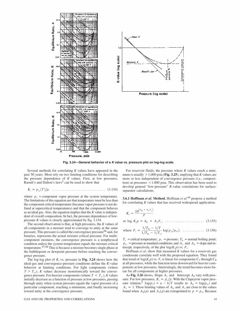
GAS AND OIL PROPERTIES AND CORRELATIONS 41
Fig. 3.24—General behavior of a K value vs. pressure plot on log-log scale.
Several methods for correlating K values have appeared in thepast 50 years. Most rely on two limiting conditions for describingthe pressure dependence of K values. First, at low pressures,Raoult’s and Dalton’s laws3 can be used to show that
Ki� pvi�T ��p, (3.154). . . . . . . . . . . . . . . . . . . . . . . . . . . . . .
where pv�component vapor pressure at the system temperature.The limitations of this equation are that temperature must be less thanthe component critical temperature (because vapor pressure is not de-fined at supercritical temperatures) and that the component behavesas an ideal gas. Also, the equation implies that the K value is indepen-dent of overall composition. In fact, the pressure dependence of low-pressure K values is closely approximated by Eq. 3.154.
The second observation is that, at high pressures, the K values ofall components in a mixture tend to converge to unity at the samepressure. This pressure is called the convergence pressure96 and, forbinaries, represents the actual mixture critical pressure. For multi-component mixtures, the convergence pressure is a nonphysicalcondition unless the system temperature equals the mixture criticaltemperature.97,98 This is because a mixture becomes single phase atthe bubblepoint or dewpoint pressure before reaching the conver-gence pressure.
The log-log plot of Ki vs. pressure in Fig. 3.24 shows how theideal-gas and convergence-pressure conditions define the K-valuebehavior at limiting conditions. For light components (whereT� Tci ), K values decrease monotonically toward the conver-gence pressure. For heavier components (where T� Tci ), K valuesinitially decrease as a function of pressure at low pressures, passingthrough unity when system pressure equals the vapor pressure of aparticular component, reaching a minimum, and finally increasingtoward unity at the convergence pressure.
For reservoir fluids, the pressure where K values reach a mini-mum is usually �1,000 psia (Fig. 3.25), implying that K values aremore or less independent of convergence pressure (i.e., composi-tion) at pressures �1,000 psia. This observation has been used todevelop general “low-pressure” K-value correlations for surface-separator calculations.
3.6.1 Hoffman et al. Method. Hoffman et al.99 propose a methodfor correlating K values that has received widespread application.
Ki�10�A0 � A1 Fi
�
p
or log Ki p� A0 � A1 Fi , (3.155). . . . . . . . . . . . . . . . . . . . . .
where Fi�1�Tbi� 1�T
1�Tbi� 1�Tcilog�pci�psc�; (3.156). . . . . . . . . . . .
Tc�critical temperature; pc�pressure; Tb�normal boiling point;psc�pressure at standard conditions; and A1 and A0�slope and in-tercept, respectively, of the plot log(Ki p) vs. Fi.
Hoffman et al. show that measured K values for a reservoir gascondensate correlate well with the proposed equation. They foundthat trend of log(Ki p) vs. Fi is linear for components C1 through C6at all pressures, while the function turns downward for heavier com-ponents at low pressures. Interestingly, the trend becomes more lin-ear for all components at higher pressures.
As Fig. 3.26 shows, Slope A1 and Intercept A0 vary with pres-sure. For low pressures, Ki� pv�p. With the Clapeyron vapor pres-sure relation,5 log(pv)� a� b�T results in A0� log(psc) andA1� 1. These limiting values of A0 and A1 are close to the valuesfound when A0(p) and A1(p) are extrapolated to p� psc. Because

42 PHASE BEHAVIOR
Fig. 3.25—K values at 120°F for binary- and reservoir-fluid systems with convergence pressuresranging from 800 to 10,000 psia (from Standing3).
K values tend toward unity as pressure approaches the convergencepressure, pK , it is necessary that A0� log(pK) and A1 0. Severalauthors have noted that plots of log(Ki p) vs. Fi tend to converge ata common point. Brinkman and Sicking101 suggest that this “pivot”point represents the convergence pressure where Ki� 1 andp� pK. The value of Fi at the pivot point, FK, is easily shown toequal log(pK�psc).
It is interesting to note that the well-known Wilson102,103 equation,
Ki�exp 5.37(1� i)�1� T�1
ri�
pri, (3.157). . . . . . . . . . . . . .
is identical to the Hoffman et al.99 relation for A0� log(psc) andA1� 1 when the Edmister104 correlation for acentric factor equation,
i�37
Tbi�Tci
1� Tbi�Tcilog�pci�psc� � 1 , (3.158). . . . . . . . . . . .
is used in the Wilson equation. Note that 5.37�(7/3) ln (10).Whitson and Torp100 suggest a generalized form of the Hoffman
et al.99 equation in terms of convergence pressure and acentric factor.
Ki� �pcipK�
A1�1 exp 5.37 A1 (1� i)�1� T�1ri��
pri,
(3.159). . . . . . . . . . . . . . . . . . .
where A1�a function of pressure, with A1� 1 at p� psc andA1� 0 at p� pK. The key characteristics of K values vs. pressure

GAS AND OIL PROPERTIES AND CORRELATIONS 43
Fig. 3.26—Pressure dependence of slope, A1, and intercept, A0,in Hoffman et al. Kp-F relationship (Eq. 3.155) for a North Seagas condesate NS-1 (from Whitson and Torp100).
Pressure, psia
Intercept A0
Slope A1
–
log pK
and temperature are correctly predicted by Eq. 3.159, where the fol-lowing pressure dependence for A1 is suggested.
A1� 1� (p�pK)A2 , (3.160). . . . . . . . . . . . . . . . . . . . . . . . . .
where A2 ranges from 0.5 to 0.8 and pressures p and pK are givenin psig. Canfield105 also suggests a simple K-value correlationbased on convergence pressure.
3.6.2 Standing Low-Pressure K Values. Standing106 uses the Hof-fman et al.99 method to generate a low-pressure K-value equationfor surface-separator calculations ( psp� 1, 000 psia andTsp� 200�F). Standing fits A1 and A0 in Eq. 3.155 as a functionof pressure using K-value data from an Oklahoma City crude oil. Hetreats the C7� by correlating the behavior of KC7�
as a function of“effective” carbon number nC7�
. The Standing equations are
Ki�1
psp10�A0 � A1 Fi
�, (3.161a). . . . . . . . . . . . . . . . . . . . . . . .
Fi� bi�1�Tbi� 1�T�, (3.161b). . . . . . . . . . . . . . . . . . . . . . .
bi� log�pci�psc���1�Tbi� 1�Tci�, (3.161c). . . . . . . . . . . . . . .
A0�p� � 1.2� �4.5� 10�4�p� �15� 10�8�p2,
(3.161d). . . . . . . . . . . . . . . . . .
A1�p� � 0.890� �1.7� 10�4�p� �3.5� 10�8�p2,
(3.161e). . . . . . . . . . . . . . . . . . .
nC7�� 7.3� 0.0075T� 0.0016p, (3.161f). . . . . . . . . . . . .
bC7�� 1, 013� 324nC7�
� 4.256n2C7�
, (3.161g). . . . . . .
and TbC7�� 301� 59.85nC7�
� 0.971n2C7�
, (3.161h). . . . .
with T in °R except when calculating nC7� (for nC7�
, T is in °F) andp in psia. Standing suggests modified values of bi and Tbi for nonhy-drocarbons, methane, and ethane (Table 3.3). Glasø and Whitson107
show that these equations are accurate for separator flash calcula-tions of crude oils with GOR’s ranging from 300 to 1,500 scf/STBand oil gravity ranging from 26 to 48°API. Experience shows, how-ever, that significant errors in calculated GOR may result for leangas condensates, probably because of inaccurate C1 and
TABLE 3.3—VALUES OF b AND Tb FOR USE INSTANDING LOW-PRESSURE K-VALUE CORRELATION
Component, ibi
(cycle-°R)Tbi°R
N2 470 109
CO2 652 194
H2S 1,136 331
C1 300 94
C2 1,145 303
C3 1,799 416
i-C4 2,037 471
n-C4 2,153 491
i-C5 2,368 542
n-C5 2,480 557
C6 (lumped) 2,738 610
n-C6 2,780 616
n-C7 3,068 669
n-C8 3,335 718
n-C9 3,590 763
n-C10 3,828 805
For C7+ fractions, see Eqs. 3.161f through 3.161h
C7� K values. The Hoffman et al. method with Standing’s low-pres-sure correlations are particularly useful for checking the consisten-cy of separator-gas and -oil compositions.
3.6.3 Galimberti-Campbell Method. Galimberti and Camp-bell108,109 suggested another useful approach for correlating K val-ues where
log Ki� A0� A1T2ci
(3.162). . . . . . . . . . . . . . . . . . . . . . . . .
is shown to correlate K values for several simple mixtures contain-ing hydrocarbons C1 through C10 at pressures up to 3,000 psia andtemperatures from �60 to 300°F.
Whitson developed a low-pressure K-value correlation, based ondata from Roland,110 at pressures �1,000 psia and temperaturesfrom 40 to 200°F, for separator calculations of gas condensates.
A0� 4.276� �7.6� 10�4�T
� � 1.18� �5.675� 10�4�T� log p , (3.163a). . . . . . . .
A1� 10�6��� 4.9563� 0.00955T � � �1.9094� 10�3�
� �1.235� 10�5�T� �3.34� 10�8�T 2�p�, (3.163b). . .
TcC1� 343� 0.04p, (3.163c). . . . . . . . . . . . . . . . . . . . . . . . .
and TcC7� � 1, 052.5� 0.5125T� 0.00375T 2 , (3.163d). . . .
with p in psia, T in °F, and Tc in °R.
3.6.4 Nonhydrocarbon K Values. Lohrenz et al.111 reported non-hydrocarbon K values as a function of pressure, temperature, andconvergence pressure.
ln KH2S� �1� ppK�
0.8
6.3992127�1, 399.2204
T
� 0.76885112 ln p�18.215052 ln p
T
�1, 112, 446.2
T 2�, (3.164a). . . . . . . . . . . . . . . . . . . . .

44 PHASE BEHAVIOR
ln KN2� �1� p
pK�
0.4
�11.294748�1, 184.2409
T
� 0.90459907 ln p�, (3.164b). . . . . . . . . . . . . . . . . . .
ln KCO2� �1� p
pK�
0.6
�7.0201913� 152.7291T
� 1.8896974
� ln p �1, 719.2956 ln p
T�
644, 740.69 ln pT 2� ,(3.164c). . . . . . . . . . . . . . . . . . .
with p in psia and T in °R. For low-pressure K-value estimation, thefirst term in Eq. 3.164 simplifies to unity (assuming that1� p�pK� 1) and the K values become functions of pressure andtemperature only. However, these equations do not give the correctlow-pressure value of (ln Ki)�(ln p)�� 1
3.6.5 Convergence-Pressure Estimation. For correlation pur-poses, convergence pressure is used as a variable to define the com-position dependence of K values. Convergence pressure is a func-tion of overall composition and temperature. Whitson andMichelsen112 show that convergence pressure is a thermodynamicphenomenon, with the characteristics of a true mixture critical point,that can be predicted with EOS’s.
Rzasa et al.113 give an empirical correlation for convergencepressure as a function of temperature and the product (M�)C7�
.Standing2 suggests that convergence pressure of reservoir fluids va-ries almost linearly with C7� molecular weight.
Convergence pressure can also be calculated with a trial-and-er-ror procedure suggested by Rowe.97,98,114 This procedure involvesthe use of several empirical correlations for estimating mixture criti-cal pressure and temperature, pseudocomponent critical properties,and the K values of methane and octane. The Galimberti and Camp-bell108,109 K-value method is used to estimate K values of othercomponents by interpolation and extrapolation of the C1 and C8 Kvalues. This approach to convergence pressure is necessary if the Kvalues are used for processes that approach critical conditions orwhere K values change significantly because of overall compositioneffects. The method cannot, of course, be more accurate than thecorrelations it uses and therefore is expected to yield only qualita-tively correct results.
For reservoir calculations where convergence pressure can be as-sumed constant (e.g., pressure depletion), a more direct approach todetermining convergence pressure is suggested. With a K-value cor-relation of the form Ki� K(pK, p, T ) as in Eq. 3.159, the conver-gence pressure can be estimated from a single experimental satura-tion pressure. For a bubblepoint and a dewpoint, Eqs. 3.165 and3.166, respectively, must be satisfied.
F �pK� � 1��
N
i�1
zi Ki�pK, pb, T� � 0 (3.165). . . . . . . . . . . . .
and F�pK� � 1��
N
i�1
zi
Ki�pK, pd , T�� 0, (3.166). . . . . . . . . . .
where zi, pb, or pd and T are specified and pK is determined.The two-phase flash calculation, with K values given, is dis-
cussed in Chap. 4 in the Phase-Split Calculation section.
���������
1. The SI Metric System of Units and SPE Metric Standard, SPE, Richard-son, Texas (June 1982).
2. van der Waals, J.D.: “Continuity of the Gaseous and Liquid State ofMatter,” PhD dissertation, U. of Leiden (1873).
3. Standing, M.B.: Volumetric and Phase Behavior of Oil Field Hydrocar-bon Systems, SPE, Richardson, Texas (1981).
4. Standing, M.B. and Katz, D.L.: “Density of Natural Gases,” Trans.,AIME (1942) 146, 140.
5. Kay, W.B.: “Density of Hydrocarbon Gases and Vapors at High Tem-perature and Pressure,” Ind. Eng. Chem. (1936) No. 28, 1014.
6. Reid, R.C., Prausnitz, J.M., and Polling, B.E.: The Properties of Gasesand Liquids, fourth edition, McGraw-Hill Book Co. Inc., New YorkCity (1987) 388–485.
7. Sutton, R.P.: “Compressibility Factors for High-Molecular Weight Res-ervoir Gases,” paper SPE 14265 presented at the 1985 SPE AnnualTechnical Conference and Exhibition, Las Vegas, Nevada, 22–25 Sep-tember.
8. Ramey, H.J. Jr.: “Rapid Methods for Estimating Reservoir Compress-ibilities,” JPT (April 1964) 447; Trans., AIME, 231.
9. Fetkovich, M.J., Reese, D.E., and Whitson, C.H.: “Application of aGeneral Material Balance for High-Pressure Gas Reservoirs,” SPEJournal (March 1998) 3.
10. Fick, A.: Am. Phys., Leipzig (1855) 170, 59.11. Coats, K.H.: “Implicit Compositional Simulation of Single-Porosity
and Dual-Porosity Reservoirs,” paper SPE 18427 presented at the 1989SPE Symposium on Reservoir Simulation, Houston, 6–8 February.
12. da Silva, F.V. and Belery, P.: “Molecular Diffusion in Naturally Frac-tured Reservoirs—A Decisive Recovery Mechanism,” paper SPE19672 presented at the 1987 SPE Annual Technical Conference and Ex-hibition, San Antonio, Texas, 8–11 October.
13. Amyx, J.W., Bass, D.M. Jr., and Whiting, R.L.: Petroleum ReservoirEngineering, McGraw-Hill Book Co. Inc., New York City (1960).
14. Christoffersen, K. and Whitson, C.H.: “Gas/Oil Capillary Pressure ofChalk at Elevated Pressures,” SPEFE (September 1995) 153.
15. Delclaud, J., Rochon, J., and Nectoux, A.: “Investigation of Gas/OilRelative Permeabilities: High-Permeability Oil Reservoir Applica-tion,” paper SPE 16966 presented at the 1987 SPE Annual TechnicalConference and Exhibition, Dallas, 27–30 September.
16. Katz, D.L. et al.: Handbook of Natural Gas Engineering, McGraw-HillBook Co. Inc., New York City (1959) 69–93.
17. Standing, M.B.: Oil-System Correlations, P.P. Handbook (ed.),McGraw-Hill Book Co. Inc., New York City (1962).
18. Beggs, H.D.: “Oil System Correlations,” Petroleum Engineering Hand-book, SPE, Richardson, TX (1987) Chap. 22.
19. McCain, W.D. Jr.: “Reservoir-Fluid Property Correlations—State ofthe Art,” SPERE (May 1991) 266.
20. Whitson, C.H. and Torp, S.B.: “Evaluating Constant Volume DepletionData,” JPT (March 1983) 610; Trans., AIME, 275.
21. Hall, K.R. and Yarborough, L.: “A New EOS for Z-factor Calcula-tions,” Oil & Gas J. (18 June 1973) 82.
22. Yarborough, L. and Hall, K.R.: “How to Solve EOS for Z-factors,” Oil& Gas J. (18 February 1974) 86.
23. Takacs, G.: “Comparisons Made for Computer Z-factor Calculations,”Oil & Gas J. (20 December 1976) 64.
24. Dranchuk, P.M. and Abou-Kassem, J.H.: “Calculation of Z-Factors forNatural Gases Using Equations of State,” J. Cdn. Pet. Tech. (July–Sep-tember 1975) 14, No. 3, 34.
25. Brill, J.P. and Beggs, H.D.: “Two-Phase Flow in Pipes,” paper pres-ented at the U. Tulsa INTERCOMP Course, The Hague (1974).
26. Lee, B.I. and Kesler, M.G.: “A Generalized Thermodynamic Correla-tion Based on Three-Parameter Corresponding States,” AIChE J.(1975) 21, 510.
27. API Technical Data Book––Petroleum Refining, third edition, API,New York City (1977).
28. Starling, K.E., Mannan, M., and Savidge, J.L.: “Equation Predicts Super-compressibility for Wet, Sour Gases,” Oil & Gas J. (2 January 1989) 31.
29. Ely, J.F. and Hanley, H.J.M.: Ind. Eng. Chem. Fund. (1983) 22, 90.30. Wichert, E. and Aziz, K.: “Compressibility Factor of Sour Natural
Gases,” Cdn. J. Chem. Eng. (1971) 49, 267.31. Wichert, E. and Aziz, K.: “Calculate Z’s for Sour Gases,” Hydro. Proc.
(May 1972) 51, 119.32. Matthews, T.A., Roland, C.H., and Katz, D.L.: “High Pressure Gas
Measurement,” Petroleum Refiner (1942) 21, No. 6, 58.33. Standing, M.B.: Petroleum Engineering Data Book, Norwegian Inst. of
Technology, Trondheim, Norway (1974).34. Eilerts, C.K.: “Gas Condensate Reservoir Engineering, 1. The Re-
serve Fluid, Its Composition and Phase Behavior,” Oil & Gas J. (1February 1947).
35. Cragoe, C.S.: “Thermodynamic Properties of Petroleum Products,”U.S. Dept. of Commerce, Washington, DC (1929) 97.
36. Gold, D.K., McCain, W.D. Jr., and Jennings, J.W.: “An Improved Meth-od for the Determination of the Reservoir Gas Gravity for RetrogradeGases,” paper SPE 17310 presented at the 1988 SPE Permian Basin Oiland Gas Recovery Conference, Midland, Texas, 10–11 March.

GAS AND OIL PROPERTIES AND CORRELATIONS 45
37. Gold, D.K., McCain, W.D. Jr., and Jennings, J.W.: “An Improved Meth-od for the Determination of the Reservoir Gas Gravity for RetrogradeGases,” JPT (July 1989) 41, 747; Trans., AIME, 287.
38. Whitson, C.H.: “Discussion of An Improved Method for the Deter-mination of the Reservoir-Gas Specific-Gravity for Retrograde Gases,”JPT (November 1989) 1216.
39. Leshikar, A.G.: “How to Estimate Equivalent Gas Volume of StockTank Condensate,” World Oil (January 1961) 108.
40. Standing, M.B.: “A Pressure-Volume-Temperature Correlation for Mix-tures of California Oils and Gases,” Drill. & Prod. Prac. (1947) 275.
41. Katz, D.L.: “Prediction of the Shrinkage of Crude Oils,” Drill. & Prod.Prac. (1942) 137.
42. Carr, N.L., Kobayashi, R., and Burrows, D.B.: “Viscosity of Hydrocar-bon Gases Under Pressure,” Trans., AIME (1954) 201, 264.
43. Dempsey, J.R.: “Computer Routine Treats Gas Viscosity as a Variable,”Oil & Gas J. (16 August 1965) 141.
44. Lee, A.L., Gonzalez, M.H., and Eakin, B.E.: “The Viscosity of NaturalGases,” JPT (August 1966) 997; Trans., AIME, 237.
45. Lucas, K.: Chem. Ing. Tech. (1981) 53, 959.46. Sage, B.H. and Olds, R.H.: “Volumetric Behavior of Oil and Gas from
Several San Joaquin Valley Fields,” Trans., AIME (1947) 170, 156.47. Eilerts, C.K.: Phase Relations of Gas Condensate Fluids, Monograph
10, U.S. Bureau of Mines, American Gas Assn., New York City (1957)1 and 2.
48. Eilerts, C.K. et al.: “Phase Relations of a Gas-Condensate Fluid atLow Tempertures, Including the Critical State,” Pet. Eng. (February1948) 19, 154.
49. Nemeth, L.K. and Kennedy, H.T.: “A Correlation of Dewpoint PressureWith Fluid Composition and Temperature,” SPEJ (June 1967) 99; Trans.,AIME, 240.
50. Organick, E.I. and Golding, B.H.: “Prediction of Saturation Pressuresfor Condensate-Gas and Volatile-Oil Mixtures,” Trans., AIME (1952)195, 135.
51. Kurata, F. and Katz, D.L.: “Critical Properties of Volatile HydrocarbonMixtures,” Trans., AIChE (1942) 38, 995.
52. Glasø, O.: “Generalized Pressure/Volume/Temperature Correlations,”JPT (November 1980) 785.
53. Lasater, J.A.: “Bubblepoint Pressure Correlation,” Trans., AIME(1958) 213, 379.
54. Sutton, R.P. and Farshad, F.F.: “Evaluation of Empirically Derived PVTProperties for Gulf of Mexico Crude Oils,” SPERE (February 1990) 79.
55. Whitson, C.H.: “Characterizing Hydrocarbon Plus Fractions,” paperSPE 12233 presented at the 1980 SPE European Offshore PetroleumConference, London, 21–24 October.
56. Whitson, C.H.: “Characterizing Hydrocarbon Plus Fractions,” SPEJ(August 1983) 683; Trans., AIME, 275.
57. Vazquez, M. and Beggs, H.D.: “Correlations for Fluid Physical Proper-ty Prediction,” JPT (June 1980) 968.
58. Standing, M.B. and Katz, D.L.: “Density of Crude Oils Saturated WithNatural Gas,” Trans., AIME (1942) 146, 159.
59. Madrazo, A.: “Liquid-Density Correlation of Hydrocarbon Systems,”Trans., AIME (1960) 219, 386.
60. Vogel, J.L. and Yarborough, L.: “The Effect of Nitrogen on the PhaseBehavior and Physical Properties of Reservoir Fluids,” paper SPE 8815presented at the 1980 SPE Annual Technical Conference and Exhibi-tion, Tulsa, Oklahoma, 20–23 April.
61. Alani, G.H. and Kennedy, H.T.: “Volumes of Liquid Hydrocarbons atHigh Temperatures and Pressures,” Trans., AIME (1960) 219, 288.
62. Lohrenz, J., Bray, B.G., and Clark, C.R.: “Calculating Viscosities ofReservoir Fluids From Their Compositions,” JPT (October 1964)1171; Trans., AIME, 231.
63. Rackett, H.G.: “EOS for Saturated Liquids,” J. Chem. Eng. Data (1970)15, No. 4, 514.
64. Hankinson, R.W. and Thomson, G.H.: “A New Correlation for SaturatedDensities of Liquids and Their Mixtures,” AIChE J. (1979) 25, No. 4, 653.
65. Hankinson, R.W. et al.: “Volume Correction Factors for LubricatingOils,” Oil & Gas J. (28 September 1981) 297.
66. Cullick, A.S., Pebdani, F.N., and Griewank, A.K.: “Modified Corre-sponding States Method for Predicting Densities of Petroleum Reser-voir Fluids,” paper presented at the 1988 AIChE Spring Natl. Meeting,New Orleans, 7–10 March.
67. Chien, M.C.H. and Monroy, M.R.: “Two New Density Correlations,”paper SPE 15676 presented at the 1976 SPE Annual Technical Confer-ence and Exhibition, New Orleans, 5–8 October.
68. Ahmed, T.: Hydrocarbon Phase Behavior, first edition, Gulf Publish-ing Co., Houston (1989) 7.
69. Craft, B.C. and Hawkins, M.: Applied Petroleum Reservoir Engi-neering, first edition, Prentice-Hall, Englewood Cliffs, New Jersey(1959) 126–29.
70. Trube, A.S.: “Compressibility of Undersaturated Hydrocarbon Reser-voir Fluids,” Trans., AIME (1957) 210, 241.
71. Al-Marhoun, M.A.: “New Correlations for FVFs of Oil and Gas Mix-tures,” PhD dissertation, King Fahd U. of Petroleum & Minerals (1990).
72. Beal, C.: “The Viscosity of Air, Water, Natural Gas, Crude Oil and ItsAssociated Gases at Oilfield Temperatures and Pressures,” Trans.,AIME (1946) 165, 94.
73. Beggs, H.D. and Robinson, J.R.: “Estimating the Viscosity of Crude OilSystems,” JPT (September 1975) 1140.
74. Al-Khafaji, A.H., Abdul-Majeed, G.H., and Hassoon, S.F.: “ViscosityCorrelation for Dead, Live, and Undersaturated Crude Oils,” J. Pet.Res. (1987) 6, No. 2, 1.
75. Standing, M.B.: “UOP Characterization Factor,” TI program listing,available from C.H. Whitson, Norwegian Inst. of Science and Technol-ogy, NTNU, [email protected].
76. Chew, J.N. and Connally, C.A.: “A Viscosity Correlation for Gas-Satu-rated Crude Oils,” Trans., AIME (1959) 216, 23.
77. Aziz, K., Govier, G.W., and Fogarasi, M.: “Pressure Drop in Wells Pro-ducing Oil and Gas,” J. Cdn. Pet. Tech. (July–September 1972) 38.
78. Abu-Khamsin, S.A. and Al-Marhoun, M.A.: “Development of a NewCorrelation for Bubblepoint Oil Viscosity,” Arabian J. Sci. & Eng.(April 1991) 16, No. 2A, 99.
79. Simon, R., Rosman, A., and Zana, E.: “Phase-Behavior Properties ofCO2-Reservoir Oil Systems,” SPEJ (February 1978) 20.
80. Abdul-Majeed, G.H., Kattan, R.R., and Salman, N.H.: “New Correla-tion for Estimating the Viscosity of Undersaturated Crude Oils,” J. Cdn.Pet. Tech. (May–June 1990) 29, No. 3, 80.
81. Khan, S.A. et al.: “Viscosity Correlations for Saudi Arabian CrudeOils,” paper SPE 15720 presented at the 1987 SPE Middle East OilTechnical Conference and Exhibition, Manama, Bahrain, 8–10 March.
82. Jossi, J.A., Stiel, L.I., and Thodos, G.: “The Viscosity of Pure Substancesin the Dense Gaseous and Liquid Phases,” AIChE J. (1962) 8, 59.
83. Stiel, L.I. and Thodos, G.: “The Viscosity of Nonpolar Gases at NormalPressures,” AIChE J. (1961) 7, 611.
84. Weinaug, C.F. and Katz, D.L.: “Surface Tensions of Methane-PropaneMixtures,” Ind. & Eng. Chem. (1943) 35, 239.
85. Macleod, D.B.: “On a Relation Between Surface Tension and Density,”Trans., Faraday Soc. (1923) 19, 38.
86. Nokay, R.: “Estimate Petrochemical Properties,” Chem. Eng. (23 Feb-ruary 1959) 147.
87. Katz, D.L. and Saltman, W.: “Surface Tension of Hydrocarbons,” Ind.& Eng. Chem. (January 1939) 31, 91.
88. Katz, D.L., Monroe, R.R., and Trainer, R.P.: “Surface Tension of CrudeOils Containing Dissolved Gases,” Pet. Tech. (September 1943).
89. Standing, M.B. and Katz, D.L.: “Vapor-Liquid Equilibria of NaturalGas-Crude Oil Systems,” Trans., AIME (1944) 155, 232.
90. Firoozabadi, A. et al.: “Surface Tension of Reservoir Crude-Oil/GasSystems Recognizing the Asphalt in the Heavy Fraction,” SPERE (Feb-ruary 1988) 265.
91. Ramey, H.J. Jr.: “Correlations of Surface and Interfacial Tensions ofReservoir Fluids,” paper SPE 4429 available from SPE, Richardson,Texas (1973).
92. Wilke, C.R.: “A Viscosity Equation for Gas Mixtures,” J. Chem. Phy.(1950) 18, 517.
93. Sigmund, P.M.: “Prediction of Molecular Diffusion at Reservoir Condi-tions. Part I—Measurement and Prediction of Binary Dense Gas Diffu-sion Coefficients,” J. Cdn. Pet. Tech. (April–June 1976) 48.
94. Christoffersen, K.: “High-Pressure Experiments with Application toNaturally Fractured Chalk Reservoirs. 1. Constant Volume Diffusion.2. Gas-Oil Capillary Pressure,” Dr.Ing. dissertation, U. Trondheim,Trondheim, Norway (1992).
95. Renner, T.A.: “Measurement and Correlation of Diffusion Coefficientsfor CO2 and Rich-Gas Applications,” SPERE (May 1988) 517; Trans.,AIME, 285.
96. Hadden, S.T.: “Convergence Pressure in Hydrocarbon Vapor-LiquidEquilibra,” Chem. Eng. Prog. (1953) 49, No. 7, 53.
97. Rowe, A.M. Jr.: “Applications of a New Convergence Pressure Con-cept to the Enriched Gas Drive Process,” PhD dissertation, U. of Texas,Austin, Texas (1964).
98. Rowe, A.M. Jr.: “The Critical Composition Method—A New Conver-gence Pressure Method,” SPEJ (March 1967) 54; Trans., AIME, 240.
99. Hoffmann, A.E., Crump, J.S., and Hocott, C.R.: “EquilibriumConstants for a Gas-Condensate System,” Trans., AIME (1953) 198, 1.

46 PHASE BEHAVIOR
100. Whitson, C.H. and Torp, S.B.: “Evaluating Constant Volume DepletionData,” JPT (March 1983) ; Trans., AIME, 275.
101. Brinkman, F.H. and Sicking, J.N.: “Equilibrium Ratios for ReservoirStudies,” Trans., AIME (1960) 219, 313.
102. Wilson, G.M.: “Calculation of Enthalpy Data From a Modified Re-dlich-Kwong EOS,” Advances in Cryogenic Eng. (1966) 11, 392.
103. Wilson, G.M.: “A Modified Redlich-Kwong EOS, Application to Gen-eral Physical Data Calculations,” paper 15c presented at the 1969AIChE Natl. Meeting, Cleveland, Ohio.
104. Edmister, W.C.: “Applied Hydrocarbon Thermodynamics, Part 4: Com-pressibility Factors and Equations of State,” Pet. Ref. (April 1958) 37, 173.
105. Canfield, F.B.: “Estimate K-Values with the Computer,” Hydro. Proc.(April 1971) 137.
106. Standing, M.B.: “A Set of Equations for Computing Equilibrium Ratiosof a Crude Oil/Natural Gas System at Pressures Below 1,000 psia,” JPT(September 1979) 1193.
107. Glasø, O. and Whitson, C.H.: “The Accuracy of PVT Parameters Cal-culated From Computer Flash Separation at Pressures Less Than 1,000psia,” JPT (August 1980) 1811.
108. Galimberti, M. and Campbell, J.M.: “Dependence of Equilibrium Va-porization Ratios (K-Values) on Critical Temperature,” Proc., 48thNGPA Annual Convention (1969) 68.
109. Galimberti, M. and Campbell, J.M.: “New Method Helps Correlate KValues for Behavior of Paraffin Hydrocarbons,” Oil & Gas J. (Novem-ber 1969) 64.
110. Roland, C.H.: “Vapor Liquid Equilibrium for Natural Gas-Crude OilMixtures,” Ind. & Eng. Chem. (1945) 37, 930.
111. Lohrenz, J., Clark, G.C., and Francis, R.J.: “A Compositional MaterialBalance for Combination Drive Reservoirs With Gas and Water Injec-tion,” JPT (November 1963) 1233; Trans., AIME, 228.
112. Whitson, C.H. and Michelsen, M.L.: “The Negative Flash,” FluidPhase Equilibria (1989) 53, 51.
113. Rzasa, M.J., Glass, E.D., and Opfell, J.B.: “Prediction of Critical Prop-erties and Equilibrium Vaporization Constants for Complex Hydrocar-bon Systems,” Chem. Eng. Prog. (1952) 2, 28.
114. Rowe, A.M. Jr.: “Internally Consistent Correlations for PredictingPhase Compositions for Use in Reservoir Composition Simulators,”paper SPE 7475 presented at the 1978 SPE Annual Technical Confer-ence and Exhibition, Houston, 1–3 October.
*� ����� ��������� $�����
�1.0* E�01�nm���� ������ ������� �g/cm3
bar�1.0* E�05�Pabbl�1.589 873 E�01�m3
Btu/lbm mol�2.236 E�03�J/molcp�1.0* E�03�Pas
cSt�1.0* E�06�m2/sdyne/cm�1.0* E�00�mN/m
ft�3.048* E�01�mft2�9.290 304* E�02�m2
ft3�2.831 685 E�02�m3
ft3/lbm mol�6.242 796 E�02�m3/kmol°F (°F�32)/1.8 �°C°F (°F�459.67)/1.8 �K
in.2�6.451 6* E�00�cm2
lbm�4.535 924 E�01�kglbm mol�4.535 924 E�01�kmol
psi�6.894 757 E�00�kPapsi�1�1.450 377 E�01�kPa�1
°R�5/9 ��
*Conversion factor is exact.