currikicdn.s3-us-west-2.amazonaws.com · Contents Preface vii 1 Natural Numbers 1 1.1 Peano’s...
186
Numbers C. M. Lund June 27, 2011
Transcript of currikicdn.s3-us-west-2.amazonaws.com · Contents Preface vii 1 Natural Numbers 1 1.1 Peano’s...

Numbers
C. M. Lund
June 27, 2011

ii
Copyright c© 2011 by Carl M. Lund
History. The first stable release of this book was dated November 10, 2006.Since it is relatively easy to update an electronic version of a manuscript,we anticipate changes relatively often compared to editions of a printedmanuscript. We have therefore added this listing of page numbers (refer-ring to page numbers identifying the beginning of changes in the currentrelease) within sections where the current release differs from previous re-lease as dated below. If your copy is several releases earlier, you shouldalso consider changes in all later releases.
November 10, 2006, 5, 13, 109, 113, 115, 153, 168.
November 20, 2009, 5, 17, 19, 21, 24, 45, 48, 73, 74.
March 2, 2010, 112, 123, 129, 141, 152, 153, 158.
July 14, 2010, 61, 66, 71, 121, 122, 124, 134, 144, 151.
May 18, 2011, 4, 7, 9, 69.
Contents
Preface vii
1 Natural Numbers 11.1 Peano’s Axioms and the Natural Numbers . . . . . . . . . . 11.2 Positional Systems and Decimal Numbers . . . . . . . . . . . 41.3 Addition and Multiplication . . . . . . . . . . . . . . . . . . . 121.4 A Representation of Decimal Numbers . . . . . . . . . . . . . 171.5 Decimal Addition and Multiplication . . . . . . . . . . . . . 201.6 Ordering Property and Cancellation . . . . . . . . . . . . . . 261.7 Well-Ordering Property . . . . . . . . . . . . . . . . . . . . . 271.8 Summary . . . . . . . . . . . . . . . . . . . . . . . . . . . . . . 281.9 Appendix . . . . . . . . . . . . . . . . . . . . . . . . . . . . . 29
2 Integers 372.1 Zero . . . . . . . . . . . . . . . . . . . . . . . . . . . . . . . . . 372.2 Negative Numbers . . . . . . . . . . . . . . . . . . . . . . . . 392.3 Operations with Negative Numbers . . . . . . . . . . . . . . 402.4 An Alternate Approach . . . . . . . . . . . . . . . . . . . . . . 432.5 Decimal Subtraction . . . . . . . . . . . . . . . . . . . . . . . 452.6 The Fundamental Theorem of Arithmetic . . . . . . . . . . . 502.7 Abstract Characterization of Integers . . . . . . . . . . . . . . 522.8 Constructing the Integers . . . . . . . . . . . . . . . . . . . . 542.9 Summary . . . . . . . . . . . . . . . . . . . . . . . . . . . . . . 602.10 Appendix . . . . . . . . . . . . . . . . . . . . . . . . . . . . . 61
3 Rational Numbers 653.1 Multiplicative Inverses . . . . . . . . . . . . . . . . . . . . . . 663.2 Order and Multiplicative Inverses . . . . . . . . . . . . . . . 673.3 Operations with Multiplicative Inverses . . . . . . . . . . . . 68
iii

iv CONTENTS
3.4 Fractions . . . . . . . . . . . . . . . . . . . . . . . . . . . . . . 693.5 Decimal Fractions . . . . . . . . . . . . . . . . . . . . . . . . . 733.6 Division for Positional Systems . . . . . . . . . . . . . . . . . 743.7 Abstract Characterization of Rationals . . . . . . . . . . . . . 803.8 Constructing the Rationals . . . . . . . . . . . . . . . . . . . . 813.9 Summary . . . . . . . . . . . . . . . . . . . . . . . . . . . . . . 82
4 Real Numbers 854.1 Sequences . . . . . . . . . . . . . . . . . . . . . . . . . . . . . 854.2 Irrational Numbers . . . . . . . . . . . . . . . . . . . . . . . . 884.3 Applications . . . . . . . . . . . . . . . . . . . . . . . . . . . . 894.4 Constructing the Reals . . . . . . . . . . . . . . . . . . . . . . 944.5 Summary . . . . . . . . . . . . . . . . . . . . . . . . . . . . . . 102
5 Complex Numbers 1055.1 The Square Root of Negative One . . . . . . . . . . . . . . . . 1055.2 Addition and Multiplication . . . . . . . . . . . . . . . . . . . 1065.3 Pythagorean Theorem . . . . . . . . . . . . . . . . . . . . . . 1085.4 Geometry of Complex Numbers . . . . . . . . . . . . . . . . 1095.5 Calculating Pi . . . . . . . . . . . . . . . . . . . . . . . . . . . 1155.6 Abstract Properties . . . . . . . . . . . . . . . . . . . . . . . . 1205.7 Roots of Complex Numbers . . . . . . . . . . . . . . . . . . . 1215.8 Quadratic Equations . . . . . . . . . . . . . . . . . . . . . . . 1225.9 The Fundamental Theorem of Algebra. . . . . . . . . . . . . 1235.10 Summary . . . . . . . . . . . . . . . . . . . . . . . . . . . . . . 127
A Addendum 129A.1 Exponential and Logarithmic Tables . . . . . . . . . . . . . . 129A.2 Natural Logarithms . . . . . . . . . . . . . . . . . . . . . . . . 134A.3 Defining Property of Exponentials . . . . . . . . . . . . . . . 137A.4 Existence of Limit for Real Numbers . . . . . . . . . . . . . . 139A.5 The Exponential Property . . . . . . . . . . . . . . . . . . . . 142A.6 General Power Function . . . . . . . . . . . . . . . . . . . . . 144A.7 Exponentials for Complex Arguments . . . . . . . . . . . . . 145A.8 Logarithms . . . . . . . . . . . . . . . . . . . . . . . . . . . . . 147A.9 The Binomial Theorem . . . . . . . . . . . . . . . . . . . . . . 153A.10 Infinite Power Series . . . . . . . . . . . . . . . . . . . . . . . 157A.11 The Exponential Function exp(z) . . . . . . . . . . . . . . . . 159A.12 An Application - Loan Amortization . . . . . . . . . . . . . . 165A.13 Summary . . . . . . . . . . . . . . . . . . . . . . . . . . . . . . 170

CONTENTS v
Bibliography 171
Notation 173
Index 175

vi CONTENTS
Preface
This book is designed to give a thorough, unified treatment of basic math-ematics. Mathematics requires a careful exposition in part because it isconcerned with infinite (unlimited) sets of objects.
This book takes an engineering approach. The basic properties of thesimplest system of numbers, the natural numbers, are developed first, andmore general number systems are explicitly developed in terms of them.This highlights the unity and consistency of a wide range of topics. Specialcare is given to motivating, stating, and proving all of the material pre-sented. Motivation provides a basis for believing that the axioms, whichare the fundamentally unprovable basic assumptions of the subject, aretrue. Theorems are then shown to be the consequences of the axioms. Theproofs are given in detail, so that readers with various backgrounds can findexplanations at the appropriate level. Arguments with which the reader isalready familiar can be skimmed without loss of continuity.
Numbers arise from practical problems in describing certain basic prop-erties of collections of objects. For example, a natural number can be as-signed to a collection of objects. The properties of natural numbers allowone to infer relations between different sets of similar objects; e.g., theirrelative sizes. In the first chapter, the abstract properties of the naturalnumbers are developed by considering the abstract properties of a stringof beads when used for counting. The operations of addition and multi-plication are first motivated and given intuitive meaning by consideringthe beaded-string representation. Formal proofs are given in an appendixshowing how one gives more rigorous arguments when intuition is notconclusive. The properties of the natural numbers, and the specific formoperations such as addition and multiplication take, are illustrated by con-sidering the decimal number system as a special case. Thus the discussionproceeds from the description of the practical problem of counting, to theabstract properties of any system that might be used for counting, to itsrelationship to a specific system.
vii
viii PREFACE
The integers are discussed in the second chapter as an extension of thenatural numbers that allows the count of a number of objects to decrease aswell as increase. This is accomplished by the introduction of the negativeintegers, or additive inverses of the natural numbers. This also leads to thedefinition of zero as the sum of a natural number and its additive inverse.Addition and multiplication are defined so that the integers taken togetherobey the same associative, commutative and distributive properties as thenatural numbers alone. It is shown that this is logically possible by definingthe integers in terms of ordered pairs of natural numbers.
Similarly, in the third chapter the rational numbers are developed as anextension of the integers through the addition of multiplicative inverses. Ineffect, this allows numbers to be used for measurement as well as counting.We examine the consequences for the order property, as well as show thatthe rational numbers are logically consistent by considering them as anordered pair of integers.
The fourth chapter introduces the real numbers. We discuss why thereals are necessary to represent quantities (like the square root of two)that cannot be represented as rational numbers, even though they can beapproximated as accurately as desired. The reals are constructed such thatthe rational numbers are a subset of the reals.
The last chapter introduces the complex numbers by expanding the realsto include an element whose square is negative unity. It comes somewhatas a surprise that this introduces a two-dimensional mathematical spacesimilar to the usual physical space of two dimensions, in which the trigono-metric functions can be defined, the Pythagorean Theorem holds, and thevalue of π can be calculated. The formal properties of complex numbersare show to follow their representation as an ordered pair of real numbers.
Finally, there is an Addendum where the properties of exponentialsand logarithms of real and complex numbers are discussed. This topicis used as a background to introduce some other subjects, such as theBinomial Theorem and infinite power series, that are very useful in appliedmathematics, science, and engineering.
It is a pleasure to acknowledge many useful conversations with CathyGosler, Michael Nakamaye and Reuben Hersh of the University of NewMexico Mathematics Department. The author also benefited from discus-sions with Bill Chandler, Tom Oliphant, Pansy Stone, and Michael Lund.He is indebted to a careful reading of the manuscript by Kaylee Tejeda. Asone would expect, however, final responsibility is the author’s.
Chapter 1
Natural Numbers
We have to take advantage of a different aspect of increasing the count.A primary function of numbers is to provide an indication of the size
of a collection of objects. Basically, this is what we mean by “counting.”We illustrate counting by comparing a string of beads to the objects beingcounted. The position of the last bead identified with an object in the groupgives an indication of the size of the group.
The abstract properties of this string of beads, along with operationsusing the string, define the natural, or counting, numbers, and the associ-ated operations of addition and multiplication. Since all numbers can beconsidered basically to be built from the natural numbers, a thorough un-derstanding of the natural number system is useful in understanding othermathematical systems as well.
1.1 Peano’s Axioms and the Natural Numbers
What are the minimum assumptions necessary to describe the natural num-bers? That is, one realizes that the natural numbers are going to have certainproperties that one can’t prove. This has to be accepted, and one states ax-ioms, or properties of the natural numbers that one agrees one can’t prove.But one tries to choose those to be as reasonable as possible, so that onebelieves them to be true even if they are not proven. Then all the otherproperties of the natural numbers are proven from those axioms and thelaws of logic.
The principal law of logic used is that a mathematical statement is eithertrue or false. This is not like human affairs, where things are not either blackor white; in mathematics, things are either black or white. If a statement
1
2 CHAPTER 1. NATURAL NUMBERS
group 1
group 2
group 1
group 2 extra
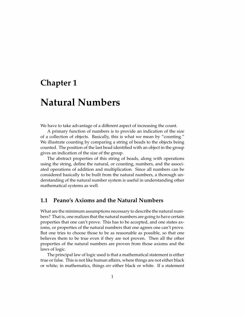
Fig. 1.1 - Comparing groups Fig. 1.2 - Comparison by counting
can be shown to contradict one of the axioms, it is false. If working fromone of the axioms we prove something is true, and working from anotherwe prove it false, then the axioms themselves are flawed, and the axiomshave to be modified.
It turns out that five axioms are sufficient to define the natural numbers.The motivation for these axioms can be appreciated by considering thenatural numbers as an infinite string of beads. This is true because one canuse a string of beads for counting.
For example, consider the simplest task in counting, determining if twogroups have the same number of elements. As shown in Fig. 1.1, one cando this by just putting the elements in a one-to-one correspondence. If onegroup has elements left over after that is done, it is larger than the other.If we put the elements of each in correspondence with the beads of a verylong (e.g., infinite) string of beads, then we know one group is larger thanthe other if there are beads between the end of one group’s beads and theend of the other (Fig. 1.2).
The five axioms we use to characterize the natural numbers were in-vented by Peano. They tell us the characteristics of the string that arenecessary so that it can be used for counting. They are
1. The set1 of natural numbers contains an element denoted 1 (one). Thisalso implies that the set is nonempty.
2. Each element x is associated with exactly one natural number, calledthe successor of x, and denoted x′.
1A set is a fundamental concept in mathematics. In some sense, it cannot be completelydefined because it is used as the building block for other concepts. You have to infer what aset is from context. Here, we just mean a set is a collection of objects. Later, we will considersets as objects themselves, and ask questions such as how we know if two sets are equal. Orhow to combine sets. One of the challenges of sets is how to handle sets with an unlimited(infinite) number of elements. We use uppercase calligraphic letters to denote sets; e.g., thesetA.
1.1. PEANO’S AXIOMS AND THE NATURAL NUMBERS 3
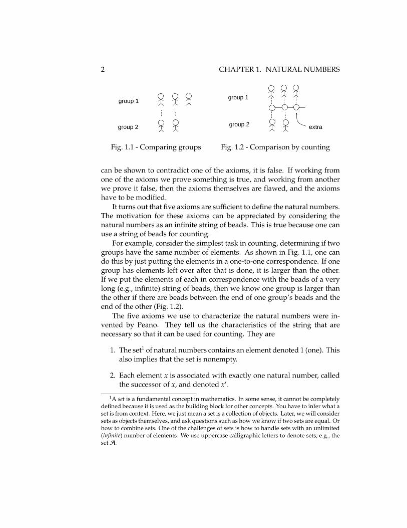
Fig. 1.3 - Useless string Fig. 1.4 - Second useless string
For our string of beads, this means the string is connected, with eachbead connected to its successor. And in particular, it is not connectedas in Fig. 1.3. Clearly, a string connected as in Fig. 1.3 would not beuseful for counting because one of its beads has two successors.
We use an arrow from a bead to its successor to illustrate this connec-tion.
3. One is the successor of no element; i.e., x′ , 1.2 This means that one isthe first bead on the string. This rules out the string in Fig. 1.4, sinceevery bead is a successor of some bead in this string.
4. If x′ = y′, then x = y; i.e., an element is the successor of at most oneelement.
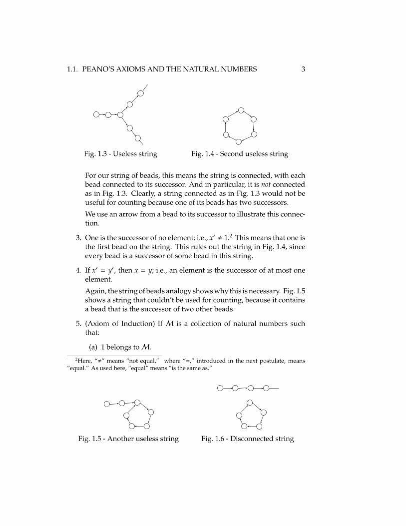
Again, the string of beads analogy shows why this is necessary. Fig. 1.5shows a string that couldn’t be used for counting, because it containsa bead that is the successor of two other beads.
5. (Axiom of Induction) If M is a collection of natural numbers suchthat:
(a) 1 belongs toM.
2Here, “,” means “not equal,” where “=,” introduced in the next postulate, means“equal.” As used here, “equal” means “is the same as.”
Fig. 1.5 - Another useless string Fig. 1.6 - Disconnected string
4 CHAPTER 1. NATURAL NUMBERS
(b) If x belongs toM then so does x′.
ThenM contains all the natural numbers.
This rules out the string in Fig. 1.6. Most people probably wouldn’tconsider Fig. 1.6 to represent a string, because, while the individualbeads are each connected to another bead, it has disconnected parts. Ifwe start with bead one, and proceeded from bead to bead by movingto each bead’s successor, we would miss the disconnected part. Thisaxiom rules out this collection for use in counting.
In addition, the Axiom of Induction is how we handle the fact that the setof natural numbers is infinite; i.e., our string of beads is without end. Itallows one to prove things about all the elements of a set even if we can’texamine each one individually.
We show how an argument by induction works by showing that everynumber except 1 has a predecessor; i.e., we show that every element except1 is the successor of some other element:
x = u′ if x , 1.
We note that this seems obvious from our string. Indeed, that’s why wedeveloped the string analogy—to give us some intuition about the natureof natural numbers. The more formal proof proceeds as follows:
(a) Let M be the set that includes one, and all numbers that are thesuccessors of some number. Clearly, one is a member ofM. (b) If x belongsto M, then we have x′ = u′ for some u if we choose u = x. That is, x′
belongs toM because it is a successor of x, and x has a successor because ofPeano’s second axiom. So x′ belongs toM. Thus by induction,M includesall natural numbers.
Note the properties of this formal proof: We are going to use the Axiomof Induction. To do that, we explicitly show that our argument satisfies thetwo requirements of the axiom. We show that the first requirement holds;namely, that the setM includes one (by definition). Then we show that thesecond requirement holds because each element has a successor by Peano’ssecond axiom. Each element of the argument holds either by definition orby reference to an axiom.
1.2 Positional Systems and Decimal Numbers
In the last section, we used a string of beads to give us a tool for indicatingthe size of a collection of objects. The beads were aligned with the objects

1.2. POSITIONAL SYSTEMS AND DECIMAL NUMBERS 5
of the collection, and the position of the last bead that was aligned withan object was a representation of the size of that collection. In this book,such a representation we will often call a “number.” But more precisely, theposition of the last bead is the representation of a number, rather than thenumber itself. As a convenience we often use the word “number” whenwe are really indicating the representation of a number. The distinction isanalogous to that in an ordinary game, such as chess. There is the abstractgame of chess with its abstract rules, and there are concrete representationswith specific boards and specific representations of the playing pieces. Anexpensive chess set (a specific representation of the game) might be highlydecorative, but a game of chess played on an inexpensive set is the sameas one played on an expensive chess set, as long as one can make theconnection between the corresponding pieces.
The numbers themselves and the rules for manipulating them are anumber system. The representation of the numbers and the rules for manip-ulating the representation are the representation of the number system. Asindicated previously, the numbers represented by the string of beads arecalled the natural numbers, and the rules for manipulating natural num-bers, together with the natural number themselves, make up the naturalnumber system.
The distinction between a number and its representation can be impor-tant when we realize that there are many representations of the naturalnumbers. The beaded string is a representation of the natural numbers.The Roman numerals that you might be familiar with (whose first few arei, ii, iii, iv, v, vi etc.) are another. Different representations have differentadvantages in different circumstances. We illustrated Peano’s axioms witha beaded string because it gives a clear representation of the necessity ofeach particular axiom. A binary system, which we will discuss in somedetail, is the underlying representation used in present-day digital comput-ers, because the building blocks of devices used to represent numbers canbe in one of two states. But the system most people use in day-to-day workis the decimal system.
In the decimal system, we use symbols to represent numbers ratherthan beads, and we have a rule to generate the successor of a numberthat is different than moving to the next bead on the string. The symbolrepresening a number is a string of simpler symbols3 (or digits), and theposition of the digits in the string is significant. Thus if xi is one of the
3It is probably no coincidence that the number of simple symbols is the same as thenumber of fingers on a person’s two hands.

6 CHAPTER 1. NATURAL NUMBERS
simpler symbols,x = xn . . . x1x0.
might represent a specific number, but interchanging xn and, say x0 willin general represent a different number (unless the digits xn and x0 are thesame). For example, 1 and 2 are simple symbols in the decimal system, and12 and 21 are representations of two natural numbers. But even thoughthey are made up of the same basic symbols, they don’t represent the samenumber because the position of the symbols is also significant. The decimalnumber system is a positional representation system.
In the decimal system, the representaion of the successor of a number isgenerated by starting at the right-most digit, x0. That digit is changed, sothat x0 runs through a sequence. When that sequence has been exhausted,x0 is reset to its initial value, and the next digit on the left is changed throughthe same sequence. The result is that changing the digit to the left only oncerepresents a whole sequence of changes to the successor. Similarly, after thatdigit has run through its sequence, a much larger sequence of successorshas been generated. The length of that sequence determines the radix ofthe number system. The decimal system has a radix of 10. As we shall see,the decimal system makes it easy to write down the results of any countingoperation, and also makes it relatively easy to do complicated calculations.
To see how this comes about, consider a simple system with only twosymbols in the sequence. This gives rise to a binary system, with a radix of2. To start, instead of using beads on a string to represent counts, we canuse marks on a piece of paper. For example,
on a piece of paper could represent the same count as the corresponding setof beads on a string.
Now group the marks by pairs. There will either be a single mark leftover, or none left over. Replace each pair by a single mark followed by a”0” if there was no mark left over, or a ”1” if there was one left over. Thus
= −→ 0.
Repeat the procedure again for the remaining marks:
0 = 0 −→ 10.
Repeat until all the marks have been replaced by either a ”0” or a ”1.”
10 −→ 110.

1.2. POSITIONAL SYSTEMS AND DECIMAL NUMBERS 7
This is the new binary representation of the original set of marks.It is clear how to recover the original set of marks. The digit on the right
represents either one mark or none. The next next digit to its left representseither twice as many as the neighboring digit , or none. Continue to the lastdigit on the left, giving for example
110 −→ { } { } { } = .
Similarly, by recalling the correspondence between the binary represen-tation and the set of marks, it is possible to see what the binary representa-tion of the successor to a number is. The successor to a set of marks is justthe set with an additional mark. If we associate that additional mark withthe right-most digit of the binary representation, we see that it will resultin a change depending on whether the right-most digit is a 0 or a 1. A 0should be changed to a 1. A 1 represents a mark that should be combinedwith the new mark to form a new pair. That new pair implies that the 0or 1 digit to its left should be modified, while the right-most 1 should bechanged to a 0.
Now the second-right-most digit should be changed according to thealgorithm we used to change the right-most digit. This changing the digitto the left of the symbol we are currently modifying is called carrying; i.e.,we are “carrying out” another mark from the current digit to the place onits left.
For example, the successor to 110 is simply 111. But the successor to 111is calculated in steps,
111′ −→ 11 {11} −→ 1 {11} 0 −→ {11} 00 −→ {1} 000 −→ 1000,
where we have indicated need for carrying by enclosing the multiple 1’sat a current position by braces. That is, in the first step a 1 is added in thefirst digit on the right. So there are now 2 1’s in the first digit place. Thisis converted to a 0 at that place, and a 1 is carried out and added to theplace to its left. Now we have two 1’s in next place, which results in a 0there with another 1 carried to the left again. This continues until no moreadjustments are necessary.
Calculating the successor to a binary number can be described succinctlywith Boolean algebra notation. Boolean algebra is a system for relating state-ments that are either true or false. If x is a Boolean variable associated witha statement, we let x = 1, mean “the statement associated with x is true,”and x = 0, mean “the statement associated with x is false.” The symbols¬x, where ¬ is the Boolean operator “not,” means “not x;” i.e., if x is true,
8 CHAPTER 1. NATURAL NUMBERS
then ¬x is false, and if x is false, ¬x is true. Using 1 and 0 to denote true andfalse, we have x = 1 implies ¬x = 0 and x = 0 implies ¬x = 1. We describecombination of Boolean variables using two other Boolean operators, “∧”(“and”) and “∨” (“or”). The statement x ∨ y (“x or y”) is true of either x ory is true, otherwise it is false. The statement a ∧ b (“x and y”) is true only ifboth x and y are true.
Boolean algebra is particularly useful in describing machinery that takesaction depending on the state of an element that has two possible values.This is, of course, how an electronic digital computer works. An electroniccomputer calculates by using transistors to switch output currents depend-ing on the values of one or two input currents. Conceptually a transistor, asused in an electronic computer, behaves like an electrical relay switch. Anelectrical relay switch makes or breaks a connection depending on whetherthere is a current in an electromagnetic coil (the relay magnet). If one con-siders current as representing 1, and no current as representing 0, one candescribe the control circuit using binary symbols.
For example, an “¬” circuit can be constructed by having the inputcurrent in the coil break the output circuit. That is, no current to the coilallows current in the output circuit, and current in the coil prevents currentin the output circuit. Similarly, two relays connected in series (i.e., twoseparate input currents driving two separate relay magnets) so that bothrelay outputs must be closed to close the output circuit mimics the Boolean“∧” operator. Two relays in parallel, so that current in either relay can closethe output circuit mimics the Boolean “∨” operator. The output currentfrom one circuit element can then drive the input to the next.
Consider now representing the successor of a binary number in Booleannotation. A binary number is represented as a sequence of digits, say xi,where i denotes the position of the digit and x←i is the digit to the left ofxi. For example, the binary number 110 has x0 = 0, x1 = 1, and x←1 = 1.Since the digits have only two possibilities, we can represent them as binaryvalues. For example, if xi = 1, we can interpret that as the Boolean statement“the ith digit is 1.”
Then to determine the new representation x′i of digit xi, we need twopieces of information: The initial value of xi, and whether there is a carryinto the ith position from its neighbor to the right. To give this second pieceof information, we introduce a carry symbol ci, which is nonzero if there isa carry into the ith position and zero otherwise. Then the prescription forcalculating x′i and whether there is a carry out of the ith position is
x′i = (xi ∧ ¬ci) ∨ (¬xi ∧ ci),

1.2. POSITIONAL SYSTEMS AND DECIMAL NUMBERS 9
c←i = xi ∧ ci.
Assuming that x0 refers to the right-most digit, one calculates the successorby choosing c0 = 1. With all the xi specified, this prescription determines x′0and c←0 = c1, which then determines all the digits and carry symbols to theleft.
We note here the use of parentheses to indicate the order in whichoperations are to be performed. The Boolean operations take two valuesand reduce them to a single value. We are to perform the operations withinparentheses first in reducing the final result to a single value, thus orderingthe operations within a calculation. In this case, the prescription reads “x′i isnonzero if either xi or the carry symbol ci is nonzero but not both; otherwiseit is zero. The carry symbol for the digit to the left is nonzero if xi and ciare both nonzero; otherwise it is zero.” Since we now know how to writethe symbol for i′ for a natural number, we may define 0′ = 1 and label thedigits of x = xn . . . x1x0 so that x←i denotes xi′ . One can work through thispresciption for the calculation of 111′ = 1000 given earlier to see how aspecific calculation goes.
Next, we would like to be able to tell, from the binary representation oftwo numbers, which one represents a larger count. For the representationas a string of beads, the larger count is represented by the longer string. Wecan’t count on this for binary numbers because there are different numbersof the same length. However, just as with the string representation of anumber, a longer binary number does represent a larger count than anyshorter binary number. This may seem obvious, but we will mention anargument that doesn’t depend on what count each position represents, butrather on the argument that it represents some count.
First note that any number represented by all ones follows any numberof the same length with zeros in some positions. For example, the four-digitnumber 1111 represent a larger count than any other four-digit numberlike 1100, because each 1 represents a count while each 0 represents theirabsence. Next note that the successor of all ones in those positions is alonger string beginning with one and followed by all zeros; i.e., the numberthat is one digit longer but represents the smallest count for a number of thatlength. For example, since 1111′ = 10000, the smallest five-digit number10000 represents a larger count than 1111.
Unlike the string representation, two binary numbers may be of thesame length, as in the example 1100 and 1111 above. However, to comparetwo numbers we can build up each number by examining the right-mostdigit first, and generating a sequence of numbers by adding more digits
10 CHAPTER 1. NATURAL NUMBERS
from the left until we generate the entire number. If we add a zero in astep in this process, the new number is the same as the previous one in thesequence, since leading zeros don’t represent any contribution to the countthe number represents (by virtue of how we form binary numbers fromthe beaded string, as above). If we add a one, the new number is longerthan the old one, and thus represents a larger count. If at this stage, onenumber of the sequence is longer than the corresponding number in theother sequence, that number is the largest generated so far.
Thus by adding one more digit from the previous number in the se-quence corresponding to each number, we will find which number (if ei-ther) is the larger so far. We keep this up until we have processed all thedigits in each number. So here’s how this works out for 1100 and 1111. Thefirst number in the sequence is 0 for the first and 1 for the second, so thesecond is larger after looking at one digit. The next in sequence is 00 and 11,and the second is still larger. Adding another digit give 100 and 111, so thesecond remains larger. The same is true when we add the fourth digit, afterwhich we are done since we’ve consider all digits in the original numbers.
We can write a Boolean expression implementing this algorithm thattells us if a number x follows y when forming successors of y. We start atthe right-most digit, as outlined above. Information from previous digitcalculations is necessary by the time we get to the left-most digit, becauseboth x and y may be the same length.
Therefore, let the Boolean variable gi = 1 mean that x comes after y ifwe only look at digits to the right of xi and yi For example, if we are lookingat x = 11011 and y = 11101, g2 tells us whether x1x0 = 11 follows y1y0 = 01(ignore any leading 0’s). Then
gi′ = (xi ∧ gi) ∨ (¬yi ∧ (xi ∨ gi)).
Thus gi′ = 1 if either both xi and gi are 1 (so it doesn’t matter what yi is),or yi = 0 and either xi = 1 (which makes gi = 1) or gi = 1 already (whichremains so even if xi = 0). One calculates the gi until both numbers haveonly 0’s remaining. If gn = 1, where n is the largest i needed to representeither number, then x represents a larger count than y.
Clearly, we also have a way of considering if x and y are equal: Ask if xcomes before y, and whether y comes before x. If neither comes before theother, they must be the same.
The decimal system is similar to the binary system, but a larger set ofsymbols is used. These symbols are strings of Arabic numerals (or decimal
1.2. POSITIONAL SYSTEMS AND DECIMAL NUMBERS 11
digits) from the set4
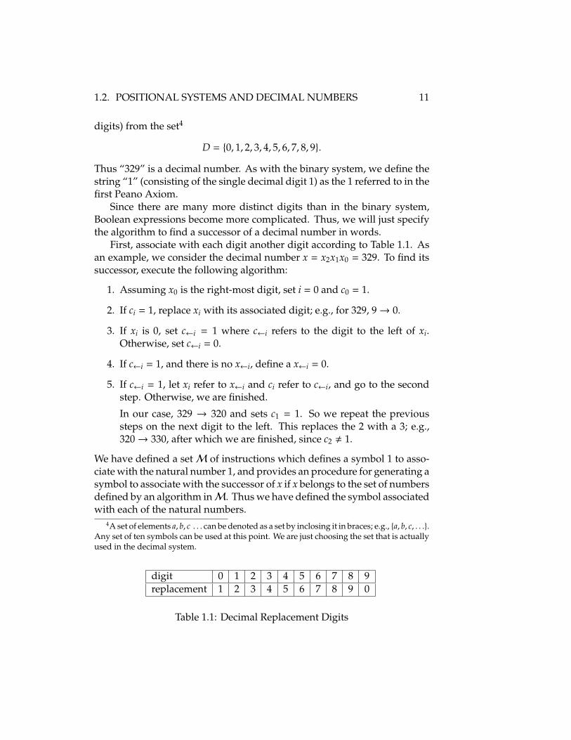
D = {0, 1, 2, 3, 4, 5, 6, 7, 8, 9}.Thus “329” is a decimal number. As with the binary system, we define thestring “1” (consisting of the single decimal digit 1) as the 1 referred to in thefirst Peano Axiom.
Since there are many more distinct digits than in the binary system,Boolean expressions become more complicated. Thus, we will just specifythe algorithm to find a successor of a decimal number in words.
First, associate with each digit another digit according to Table 1.1. Asan example, we consider the decimal number x = x2x1x0 = 329. To find itssuccessor, execute the following algorithm:
1. Assuming x0 is the right-most digit, set i = 0 and c0 = 1.
2. If ci = 1, replace xi with its associated digit; e.g., for 329, 9→ 0.
3. If xi is 0, set c←i = 1 where c←i refers to the digit to the left of xi.Otherwise, set c←i = 0.
4. If c←i = 1, and there is no x←i, define a x←i = 0.
5. If c←i = 1, let xi refer to x←i and ci refer to c←i, and go to the secondstep. Otherwise, we are finished.
In our case, 329 → 320 and sets c1 = 1. So we repeat the previoussteps on the next digit to the left. This replaces the 2 with a 3; e.g.,320→ 330, after which we are finished, since c2 , 1.
We have defined a setM of instructions which defines a symbol 1 to asso-ciate with the natural number 1, and provides an procedure for generating asymbol to associate with the successor of x if x belongs to the set of numbersdefined by an algorithm inM. Thus we have defined the symbol associatedwith each of the natural numbers.
4A set of elements a, b, c . . . can be denoted as a set by inclosing it in braces; e.g., {a, b, c, . . .}.Any set of ten symbols can be used at this point. We are just choosing the set that is actuallyused in the decimal system.
digit 0 1 2 3 4 5 6 7 8 9replacement 1 2 3 4 5 6 7 8 9 0
Table 1.1: Decimal Replacement Digits

12 CHAPTER 1. NATURAL NUMBERS
Also, it is easy to see how to modify the binary algorithm for determiningif a decimal number x can be formed by repeatly forming the successor ofthe decimal number y. And this gives us an algorithm for determining iftwo numbers are the same.
1.3 Addition and Multiplication
Rather than always counting objects by actually comparing them with astring of beads, one can define operations that allow one to combine thosebasic counting procedures to predict what one would get for a more complexcounting process. Consider an example of counting apples in two baskets.Addition is defined in such a way that if we count the apples in each basketseparately using beads, we can tell how many we would count if we putboth baskets in a larger basket and counted apples in the larger basket usingbeads.
Addition is defined inductive as follows:
1. x + 1 = x′.
2. If x + y is defined,5 then x + y′ = (x + y)′.
The first statement says that the number associated with a set when anadditional member is added to it is the successor of the number associatedwith the original set. The second statement says that if you have two sets andadd one to one of the sets, the number now associated with the combinationof the two sets is the successor of the number previously associated withthe combination.
The string-of-beads analogy is that we represent the addition of twonumbers by following one section of beads representing the first numberby a section representing the second, as shown in Fig. 1.7. (We have foregonedrawing the arrowheads from a number to its successor, since the directionof a proper string is from the initial 1.) We represent an equation by puttingthe strings side by side. If the total number of beads in each string isthe same, the expressions illustrated by the strings are equal. Here werepresent a number by a section of the string, set off with parenthesis ifnecessary for clarity. We denote a number represented as the successor of asecond number by filling in the last element. The sequence of beads ending
5Technically, it’s not obvious if we’ve defined x + y everywhere relying only on Peano’saxioms, since we only define x + y′ if x + y is already defined. See the Appendix for a moredetailed argument.

1.3. ADDITION AND MULTIPLICATION 13
(
( (
(
)2 + 1 =
2' =
3 =
)
)
)
( () )2 + 4 =
2 + 3' =
5' =
6 =
(
(
(
() )
)
)
Fig. 1.7 - x + 1 = x′ Fig. 1.8 - x + y′ = (x + y)′
in a filled bead is the number represented by all the beads. That number isthe successor of the number represented by the beads before the filled bead.In Fig. 1.7, we illustrate 2 + 1 on the top, and 3 = 2′ on the bottom.
Then Fig. 1.8 shows how we represent induction by illustrating how wedefine 2 + 4 = 6 from 2 + 3′ = 5′, where we assume that 2 + 3 = 5 has alreadybeen shown. From the representation, we see 4 as 3′ and 6 as 5′.
The real power of the analogy comes when we note from the stringanalogy that x + y = y + x, which we illustrate in Fig. 1.9. We say additionis commutative. And in Fig. 1.10, we show x + (y + z) = (x + y) + z, or thataddition is associative. We draw the figures associated with two statements,and then consider them equivalent if we can rotate or reconnect the beadsto change one into the other. So the string of beads analogy, while not aformal proof, gives us an intuitive feeling that these theorems are true. Forthose interested, we reproduce standard proofs in the Appendix.
Table 1.2 shows addition for small decimal numbers. One sees that xdefines a column and y defines a row. So for example, to calculate 6 + 8when 6 + 7 is known, we go to the column labeled 6 and the row labeled7 to get 6 + 7 = 13. 6 + 8 is the successor of 6 + 7, which our rules forgenerating successors give as 14. One can also verify that commutativityand associativity hold for numbers in this table. For example, we note that8 + 6 also equals 14.
( () )3 + 2 =
( () )2 + 3 = ( )( ) )()(
( ))( )( )((1 + 2) + 3 =
1 + (2 + 3) =
Fig. 1.9 - x + y = y + x Fig. 1.10 - x + (y + z) = (x + y) + z

14 CHAPTER 1. NATURAL NUMBERS
y\x 1 2 3 4 5 6 7 8 9 101 2 3 4 5 6 7 8 9 10 112 3 4 5 6 7 8 9 10 11 123 4 5 6 7 8 9 10 11 12 134 5 6 7 8 9 10 11 12 13 145 6 7 8 9 10 11 12 13 14 156 7 8 9 10 11 12 13 14 15 167 8 9 10 11 12 13 14 15 16 178 9 10 11 12 13 14 15 16 17 189 10 11 12 13 14 15 16 17 18 1910 11 12 13 14 15 16 17 18 19 20
Table 1.2: Decimal Addition
Next we note an interesting fact about counting with a string of beads.We have obtained a count for a set of objects, as in Fig. 1.2, by associatingeach object with a bead. But we could have associated any number of beadswith any one object and had as useful a result, as long as we associated thesame number of beads with each object. By this we mean that if we usestrings of beads to compare two sets of objects, associating x beads witheach object, we can compare the strings to find out which set is bigger evenif x isn’t a single bead.
Fig. 1.11 shows what happens when two beads are associated with oneobject. The beads thus associated will depend on two numbers, say x and y,where x is the count of beads associated with one object, and y is the countwe would have gotten if we had associated only one. Calculating the totalnumber of beads associated with y objects when each object is associatedwith x beads is called multiplication, and is described as calculating x× y. Ifone thinks a bit about it, it is clear that x × y can be defined by
1. x × 1 = x,
2. If x × y is defined,6 x × y′ = (x × y) + x.
This is very similiar to the definition of addition, but instead of increasingthe number of beads associated with a set by 1 when adding an object, oneincreases the nunber of beads by x.
Multiplication can make representing large numbers much easier. Sup-pose we consider a very simple system where we put a mark on a piece of
6See earlier footnote about the definition of addition
1.3. ADDITION AND MULTIPLICATION 15
paper for each item we count. Then as we count the first three items, wewould put down a mark in succession; i.e., , then , and finally . In thesecases, it is easy to distinguish the different case visually, as it is with thenext number . However, it is easier to be sure of the count when, at somepoint, we cross off a specific number of vertical marks. This indicates thatthe number of marks has reached a group that is about as large as can bereadily distinguished. Thus, we might chose to finish out a group of marksat, say, five, as with ¡. Then, if we add another item, the count would berepresented as ¡ + . Thus a relatively large count, of say ¡ + ¡ + , orjust ¡ ¡ , could be more readily understood that a succession of entirelysimilar marks; e.g., . . . .
In this last example we have two groups of five, plus three. Usingmultiplication to indicate this kind of grouping, we write the two groups offive as 5 × 2. Then this count is (5 × 2) + 3, where the parentheses indicatethat the number represented by 5 × 2 is determined separately, before theresult is added to 3. If we add another group of 5, then 5× 3 would replace5 × 2 in the above count.
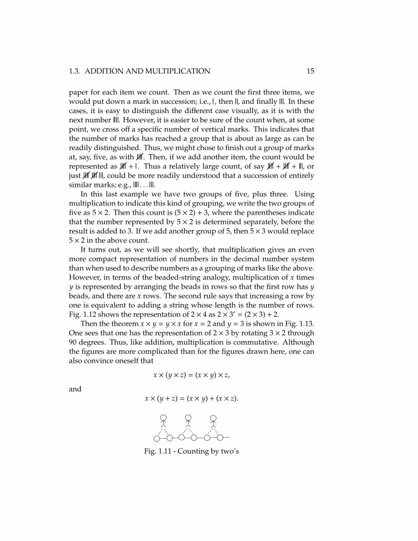
It turns out, as we will see shortly, that multiplication gives an evenmore compact representation of numbers in the decimal number systemthan when used to describe numbers as a grouping of marks like the above.However, in terms of the beaded-string analogy, multiplication of x timesy is represented by arranging the beads in rows so that the first row has ybeads, and there are x rows. The second rule says that increasing a row byone is equivalent to adding a string whose length is the number of rows.Fig. 1.12 shows the representation of 2 × 4 as 2 × 3′ = (2 × 3) + 2.
Then the theorem x× y = y× x for x = 2 and y = 3 is shown in Fig. 1.13.One sees that one has the representation of 2 × 3 by rotating 3 × 2 through90 degrees. Thus, like addition, multiplication is commutative. Althoughthe figures are more complicated than for the figures drawn here, one canalso convince oneself that
x × (y × z) = (x × y) × z,
andx × (y + z) = (x × y) + (x × z).
Fig. 1.11 - Counting by two’s

16 CHAPTER 1. NATURAL NUMBERS
(
(
(
(
(
(
)
)
)
)
)
2 x 4 =
2 x 3' =
(2 x 3) + 2 =)
(
(
)
)
(
((
)
))
2 x 3 =
3 x 2 =
Fig. 1.12 - a × b′ = (a × b) + a Fig. 1.13 - a × b = b × a
The first relation shows that multiplication is associative, and the secondrelationship shows that multiplication distributes over addition. Again, referto the Appendix for proofs.
We note that multiplication is often denoted using “·” between numbersrather than “×,” or often “×” is omitted entirely; i.e.,
x × y ≡ x · y ≡ x y,
where “≡” means “equal by definition.” Furthermore, multiplication isconsidered to have a higher precedence than addition; i.e., in an expressioninvolving combinations of multiplication and addition, without parenthe-ses to denote in which order they are to be done, all the multiplications areassumed to be done before the additions. For example
x · y′ = (x · y) + x,
can be writtenx y′ = x y + x.
Table 1.3 shows the multiplication table for small decimal numbers. Weuse it in a similar manner to the addition table, although filling it out is alittle bit more complicated. For example, we get 6 ·8 by adding 6 to 6 ·7 = 42.But 42 is not in our addition table. We proceed as follows:
42 + 6 = 42 + 5′
= 42 + (5 + 1)
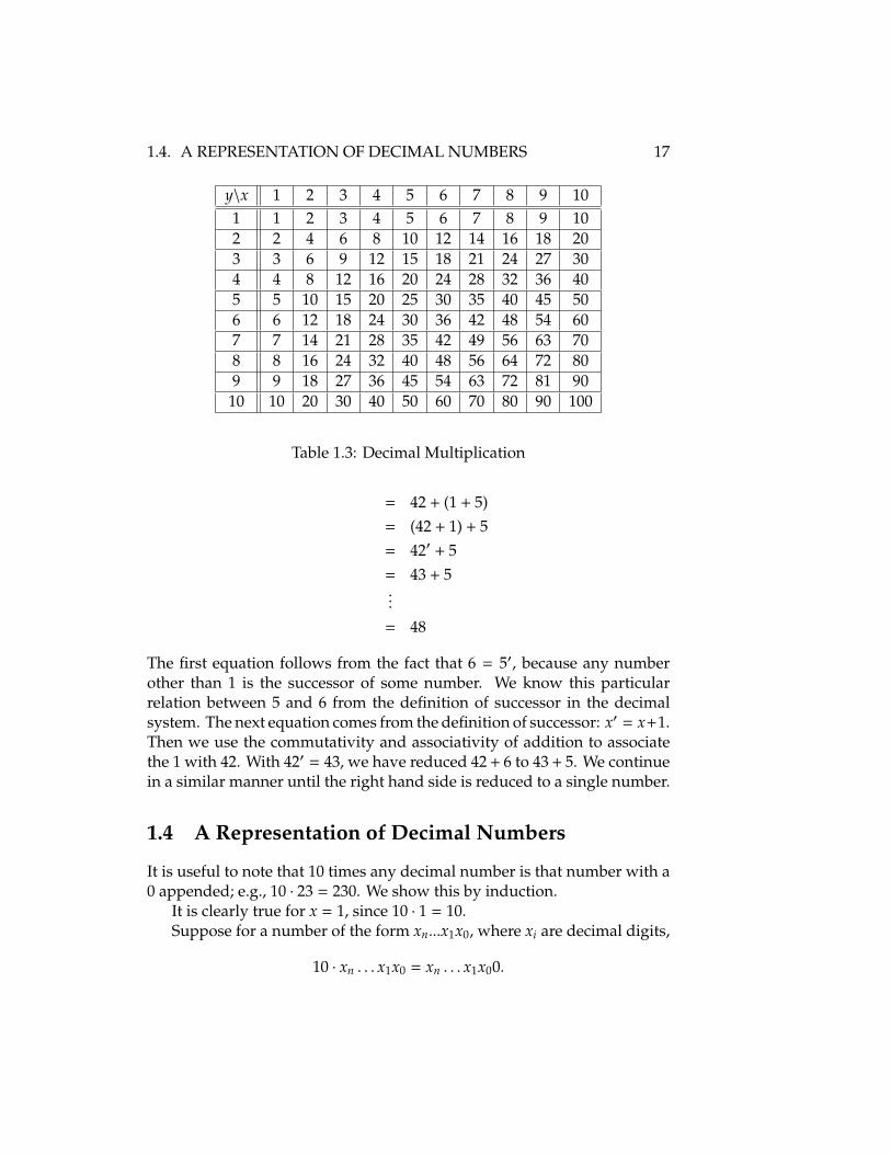
1.4. A REPRESENTATION OF DECIMAL NUMBERS 17
y\x 1 2 3 4 5 6 7 8 9 101 1 2 3 4 5 6 7 8 9 102 2 4 6 8 10 12 14 16 18 203 3 6 9 12 15 18 21 24 27 304 4 8 12 16 20 24 28 32 36 405 5 10 15 20 25 30 35 40 45 506 6 12 18 24 30 36 42 48 54 607 7 14 21 28 35 42 49 56 63 708 8 16 24 32 40 48 56 64 72 809 9 18 27 36 45 54 63 72 81 9010 10 20 30 40 50 60 70 80 90 100
Table 1.3: Decimal Multiplication
= 42 + (1 + 5)= (42 + 1) + 5= 42′ + 5= 43 + 5...
= 48
The first equation follows from the fact that 6 = 5′, because any numberother than 1 is the successor of some number. We know this particularrelation between 5 and 6 from the definition of successor in the decimalsystem. The next equation comes from the definition of successor: x′ = x+1.Then we use the commutativity and associativity of addition to associatethe 1 with 42. With 42′ = 43, we have reduced 42 + 6 to 43 + 5. We continuein a similar manner until the right hand side is reduced to a single number.
1.4 A Representation of Decimal Numbers
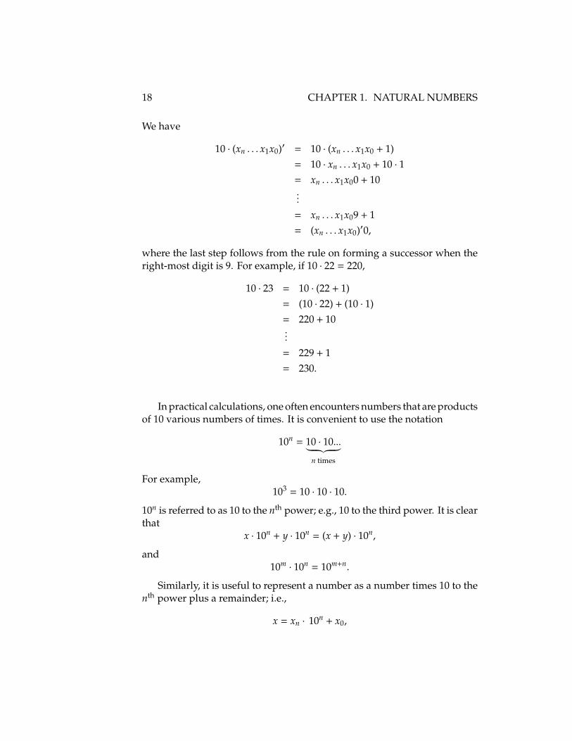
It is useful to note that 10 times any decimal number is that number with a0 appended; e.g., 10 · 23 = 230. We show this by induction.
It is clearly true for x = 1, since 10 · 1 = 10.Suppose for a number of the form xn...x1x0, where xi are decimal digits,
10 · xn . . . x1x0 = xn . . . x1x00.
18 CHAPTER 1. NATURAL NUMBERS
We have
10 · (xn . . . x1x0)′ = 10 · (xn . . . x1x0 + 1)= 10 · xn . . . x1x0 + 10 · 1= xn . . . x1x00 + 10...
= xn . . . x1x09 + 1= (xn . . . x1x0)′0,
where the last step follows from the rule on forming a successor when theright-most digit is 9. For example, if 10 · 22 = 220,
10 · 23 = 10 · (22 + 1)= (10 · 22) + (10 · 1)= 220 + 10...
= 229 + 1= 230.
In practical calculations, one often encounters numbers that are productsof 10 various numbers of times. It is convenient to use the notation
10n = 10 · 10...︸ ︷︷ ︸n times
For example,103 = 10 · 10 · 10.
10n is referred to as 10 to the nth power; e.g., 10 to the third power. It is clearthat
x · 10n + y · 10n = (x + y) · 10n,
and10m · 10n = 10m+n.
Similarly, it is useful to represent a number as a number times 10 to thenth power plus a remainder; i.e.,
x = xn · 10n + x0,
1.4. A REPRESENTATION OF DECIMAL NUMBERS 19
where x0 is a decimal digit not equal to 0. This can always be done for adecimal number not ending in 0. For example,
26 = 25 + 1...
= 20 + 6= 2 · 101 + 6
One can apply the procedure repeatedly for larger numbers; e.g.,
126 = 12 · 101 + 6= (1 · 101 + 2) · 101 + 6= 1 · 102 + 2 · 101 + 6.
Clearly, one can represent any decimal natural number as
xn . . . x1x0 = xn · 10n + . . . + x1 · 101 + x0,
if we agree to ignore terms with xi = 0, so we can handle cases like
102 = 1 · 102 + 2.
We do this by defining0 · x ≡ x · 0 ≡ 0.
We can invent an even more compact notation if we write
n∑
i=0
An = A0 + A1 + . . . + An,
and define100 ≡ 1.
Then
xn . . . x1x0 =
n∑
i=0
xi · 10i.
We can deduce a representation of binary numbers in the same way. Inthis case, we note that 2 (binary 10) times any binary number is that number
20 CHAPTER 1. NATURAL NUMBERS
with a 0 appended; e.g. 10 · 101 = 1010. And the binary number xn . . . x1x0can be written
xn . . . x1x0 =
n∑
i=0
xi · 2i.
Note that for both binary and decimal numbers, this expands a number interms of powers of the radix of the representation. With binary numbersin this representation, it is common to write the binary expression 10i as 2i,probably since decimal numbers are the choice in everyday use. If we wantto write 10 as a number to another base like 2, one often sees 102, whichreads “10 to the base 2.” In general, for any base b we might see (10b)i fordecimal 2 multiplied i times.
It is useful to note that (in decimal notation)
210 = 1024,103 = 1000.
That is, a 10-digit binary number is very nearly equivalent to a 3-digitdecimal number. So if you are used to estimating counts in decimal, youcan get an idea of the size of a count in binary by associating 10 binary digitswith every 3 decimal ones.
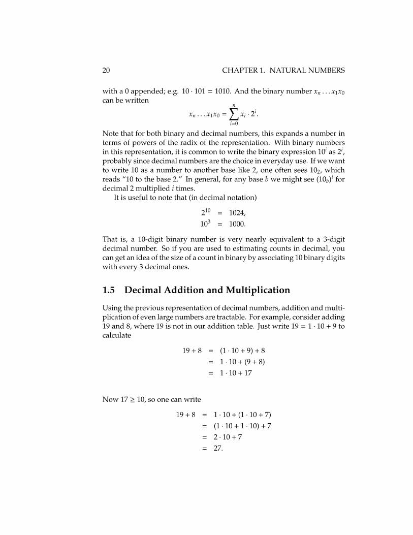
1.5 Decimal Addition and Multiplication
Using the previous representation of decimal numbers, addition and multi-plication of even large numbers are tractable. For example, consider adding19 and 8, where 19 is not in our addition table. Just write 19 = 1 · 10 + 9 tocalculate
19 + 8 = (1 · 10 + 9) + 8= 1 · 10 + (9 + 8)= 1 · 10 + 17
Now 17 ≥ 10, so one can write
19 + 8 = 1 · 10 + (1 · 10 + 7)= (1 · 10 + 1 · 10) + 7= 2 · 10 + 7= 27.

1.5. DECIMAL ADDITION AND MULTIPLICATION 21
Moving the part of 17 ≥ 10 to the position that represents coefficients of 10is called carrying.
In general, to add decimal numbers x and y, write
x =
nx∑
i=0
xi · 10i,
y =
ny∑
i=0
yi · 10i,
and form
z =
max(nx,ny)∑
i=0
(xi + yi) · 10i,
where xi = 0 if i > nx, yi = 0 if i > ny, and we define x + 0 ≡ 0 + x ≡ x (evenif x = 0). Then we adjust (normalize, using carrying) this series so that
z =
nz∑
i=0
zi · 10i.
where nz ≥ max(nx, ny), and the zi are decimal digits 0–9. We can formalizeaddition as the following algorithm:
1. Define an index number i and set i = 0. Define a “carry number ”c0 = 0.
2. Form wi = xi + yi + ci.
3. If wi ≥ 10, let wi = 10 + zi define zi and define ci′ = 1. Otherwise,define zi = wi and ci′ = 0.
4. If i < nx, i < ny, or ci′ , 0, add 1 to i and go to item 2. Otherwise, youare done.
It is usual to arrange the calculation in the following compact manner.Consider 302 + 749 as an example:
1 1
3 0 2+ 7 4 9
1 0 5 1
22 CHAPTER 1. NATURAL NUMBERS
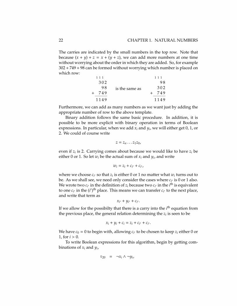
The carries are indicated by the small numbers in the top row. Note thatbecause (x + y) + z = x + (y + z), we can add more numbers at one timewithout worrying about the order in which they are added. So, for example302 + 749 + 98 can be formed without worrying which number is placed onwhich row:
1 1 1
3 0 29 8
+ 7 4 9
1 1 4 9
is the same as
1 1 1
9 83 0 2
+ 7 4 9
1 1 4 9
Furthermore, we can add as many numbers as we want just by adding theappropriate number of row to the above template.
Binary addition follows the same basic procedure. In addition, it ispossible to be more explicit with binary operation in terms of Booleanexpressions. In particular, when we add xi and yi, we will either get 0, 1, or2. We could of course write
z = zn . . . z1z0,
even if zi is 2. Carrying comes about because we would like to have zi beeither 0 or 1. So let wi be the actual sum of xi and yi, and write
wi = zi + ci′ + ci′ ,
where we choose ci′ so that zi is either 0 or 1 no matter what wi turns out tobe. As we shall see, we need only consider the cases where ci′ is 0 or 1 also.We wrote two ci′ in the definition of zi because two ci′ in the ith is equivalentto one ci′ in the (i′)th place. This means we can transfer ci′ to the next place,and write that term as
xi′ + yi′ + ci′ .
If we allow for the possibilty that there is a carry into the ith equation fromthe previous place, the general relation determining the zi is seen to be
xi + yi + ci = zi + ci′ + ci′ .
We have c0 = 0 to begin with, allowing ci′ to be chosen to keep zi either 0 or1, for i > 0.
To write Boolean expressions for this algorithm, begin by getting com-binations of xi and yi,
τ20 = ¬xi ∧ ¬yi,

1.5. DECIMAL ADDITION AND MULTIPLICATION 23
τ21 = (xi ∧ ¬yi) ∨ (¬xi ∧ yi),τ22 = xi ∧ yi,
Combine with ci,
τ31 = (τ21 ∧ ¬ci) ∨ (τ20 ∧ ci),τ32 = (τ22 ∧ ¬ci) ∨ (τ21 ∧ ci),τ33 = τ22 ∧ ci,
and calculate the result,
zi = τ31 ∨ τ33,
ci′ = τ32 ∨ τ33.
Multiplication is messier than addition for positional number systems,because we generate a lot more terms, but the basic idea is similar. We justnote, for example,
(x + y) · (z + w) = x · (z + w) + y · (z + w) = x · z + x · w + y · z + y · w.
Then
12 · 27 = (1 · 10 + 2) · (2 · 10 + 7)= 2 · 102 + 7 · 10 + 4 · 10 + 2 · 7= 2 · 102 + 11 · 10 + 14= 2 · 102 + 10 · 10 + 1 · 10 + 1 · 10 + 4= 2 · 102 + 1 · 102 + 2 · 10 + 4= 3 · 102 + 2 · 101 + 4= 324.
The general procedure is to calculate
x · y =
nx∑
i=0
xi · 10i
·
ny∑
j=0
x j · 10 j
=
nx+ny∑
n=1
∑
k,k′3k+k′=n
xk · yk′
· 10n,
24 CHAPTER 1. NATURAL NUMBERS
where “3” reads “such that,” and then normalize. The second form of theproduct comes from regrouping the outer sum to be over terms involvingthe same power of ten. For our example, the above expression gives
12 · 27 = (1 · 2) · 102 + (1 · 7 + 2 · 2) · 101 + (2 · 7) · 100,
which, of course, normalizes to 324.As a practical matter, it is easier to first note that a single-digit multiply-
ing a general number is simple to do. Write
z =
ny∑
i=0
zi · 10i = x · y =
ny∑
i=0
x · yi · 10i,
where both x and all yi are single digits. We can then use Table 1.3 for theproduct x · yi, writing it in the form ci′ · 10 + zi, where ci′ and zi are singledecimal digits. Then cn′ carrys into the calculation of x · yi′ . The generalprocedure in this case is then
1. Set i = 0 and ci = 0.
2. Calculate ci′ and zi from x · yi = ci′ · 10 + zi.
3. If i′ is less than ny, or ci′ is nonzero, set i = i′, and repeat step 2.
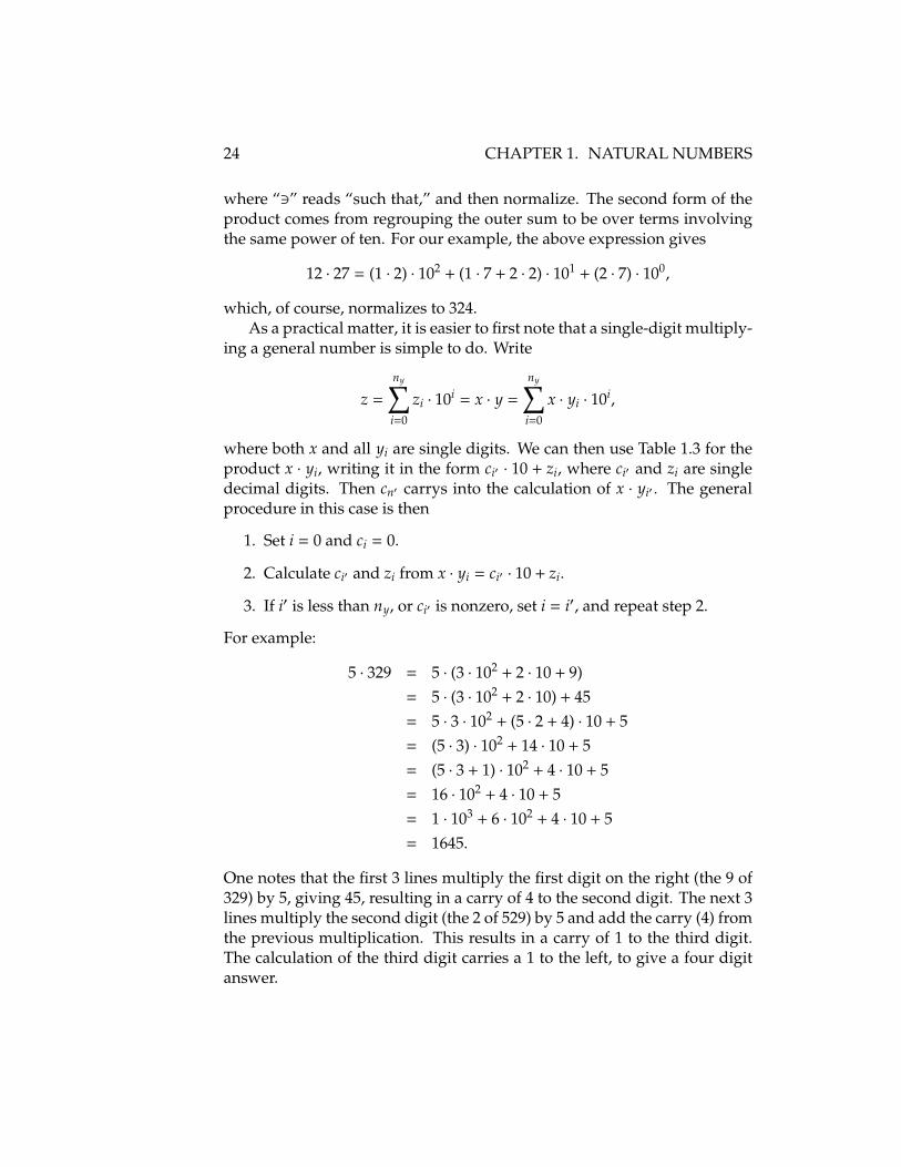
For example:
5 · 329 = 5 · (3 · 102 + 2 · 10 + 9)= 5 · (3 · 102 + 2 · 10) + 45= 5 · 3 · 102 + (5 · 2 + 4) · 10 + 5= (5 · 3) · 102 + 14 · 10 + 5= (5 · 3 + 1) · 102 + 4 · 10 + 5= 16 · 102 + 4 · 10 + 5= 1 · 103 + 6 · 102 + 4 · 10 + 5= 1645.
One notes that the first 3 lines multiply the first digit on the right (the 9 of329) by 5, giving 45, resulting in a carry of 4 to the second digit. The next 3lines multiply the second digit (the 2 of 529) by 5 and add the carry (4) fromthe previous multiplication. This results in a carry of 1 to the third digit.The calculation of the third digit carries a 1 to the left, to give a four digitanswer.
1.5. DECIMAL ADDITION AND MULTIPLICATION 25
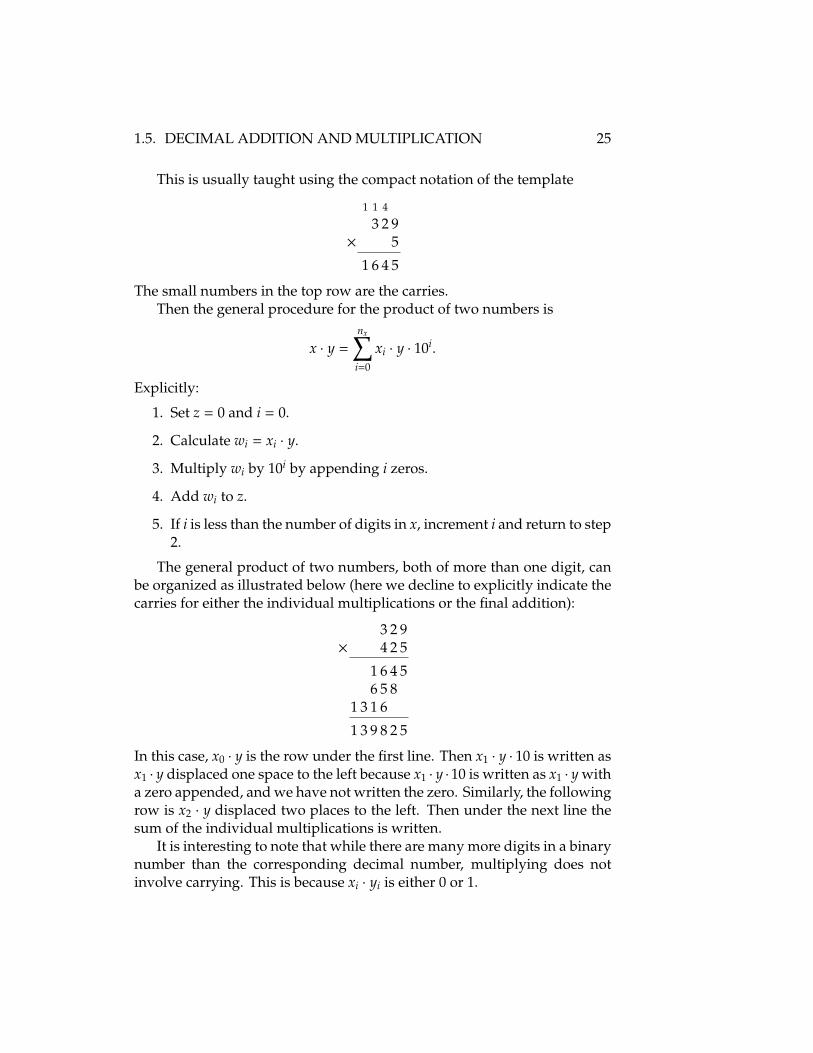
This is usually taught using the compact notation of the template
1 1 4
3 2 9× 5
1 6 4 5
The small numbers in the top row are the carries.Then the general procedure for the product of two numbers is
x · y =
nx∑
i=0
xi · y · 10i.
Explicitly:
1. Set z = 0 and i = 0.
2. Calculate wi = xi · y.
3. Multiply wi by 10i by appending i zeros.
4. Add wi to z.
5. If i is less than the number of digits in x, increment i and return to step2.
The general product of two numbers, both of more than one digit, canbe organized as illustrated below (here we decline to explicitly indicate thecarries for either the individual multiplications or the final addition):
3 2 9× 4 2 5
1 6 4 56 5 8
1 3 1 6
1 3 9 8 2 5
In this case, x0 · y is the row under the first line. Then x1 · y · 10 is written asx1 · y displaced one space to the left because x1 · y · 10 is written as x1 · y witha zero appended, and we have not written the zero. Similarly, the followingrow is x2 · y displaced two places to the left. Then under the next line thesum of the individual multiplications is written.
It is interesting to note that while there are many more digits in a binarynumber than the corresponding decimal number, multiplying does notinvolve carrying. This is because xi · yi is either 0 or 1.

26 CHAPTER 1. NATURAL NUMBERS
1.6 Ordering Property and Cancellation
Natural numbers satisfy a property that is easy to see from their similarityto a string of beads. For any natural numbers x, y, either
1. there exists a natural number u such that
x + u = y,
or
2. there exists a natural number u such that
x = y + u
or
3.
x = y.
For the first case, we write x < y or y > x (“x less than y” or “y greaterthan x”),7 and for the second case x > y or y < x. Note that these casesare mutually exclusive; for each pair x, y, there is only one possibility. Thisproperty is called order.
For example, since for all x , 1 there exists a u such that x = u′ = u + 1(or 1 + u = x), we have 1 < x. That is, 1 is the least natural number, asexpected.
This property also lets us deduce that if
a + x = a + y,
where a is a natural number, then
x = y.
For in this case, suppose a + x = a + y but x > y. Then there would exist a usuch that x = y + u. Then we would have
a + (y + u) = a + y
7Correspondingly, “≤” means “less than or equal,” and “≥” means “greater than orequal.”

1.7. WELL-ORDERING PROPERTY 27
or(a + y) + u = a + y;
i.e., a number, a + y, less than itself, which would be a contradiction.Similarly, if
a · x = a · y,with a a natural number (not zero), then
x = y.
For if x > y, for example, then we would have
a · (y + u) = a · yor
a · y + a · u = a · y,which would imply a · y is less than itself.
The theorems that x + a = y + a implies x = y, and x · a = y · a impliesx = y are called the cancellation rules.
1.7 Well-Ordering Property
It is an important property of the natural numbers that any nonempty set hasa least element. This is an additional property beyond the order propertyby itself. This is obvious from the analogy of the natural numbers with thestring of beads, but it can also be shown formally.
Let N be any nonempty set of natural numbers. LetM be the set of allnatural numbers less than or equal to every element of N . ThenM is theset of lower limits of N . Previously we showed that 1 < x for x , 1. Thus1 ∈ M (where “∈” reads “belongs to”), andM is nonempty. To show thatN has a least element, we need to show there is an element ofM that is alsoinN .
Now if m ∈ M implied m+1 ∈ M, one would have all m ∈ M by Peano’sfifth postulate. But N is nonempty. Therefore there is a m ∈ M such thatm + 1 is not in M. Then either m < n for all n ∈ N , or m ∈ N . If m < nfor all n ∈ N , then m + 1 ≤ n for all n ∈ N .8 This would put m + 1 inM,contradicting the defining property of m. Therefore, m ∈ N and m ≤ n forall n ∈ N . That is,N has a least element.
8For m < n means that there exists a u such that m + u = n. If u = 1, then m + 1 = n. Ifu , 1, then there exists some number v such that u = v′ = v + 1. Then (m + 1) + v = n, orm + 1 < n. In either case, m + 1 ≤ n.

28 CHAPTER 1. NATURAL NUMBERS
1.8 Summary
The natural numbers are defined by Peano’s axioms:
1. There is an element named “1” (one).
2. Each element x is associated with exactly one successor element, de-noted x′.
3. x′ , 1.
4. If x′ = y′, then x = y.
5. IfM is a collection of natural numbers such that
(a) 1 belongs toM,
(b) If x belongs toM, then x′ belongs toM,
thenM contains all the natural numbers (the Axiom of Induction).
It follows that each number except 1 has a predecessor u such that x = u′.The operation of addition between natural numbers is defined by
1. x + 1 = x′.
2. If x + y is defined, then x + y′ = (x + y)′.
The operation of multiplication between natural numbers is defined by
1. x × 1 = x.
2. If x × y is defined, then x × y′ = (x × y) + x.
Addition and multiplication have the following properties:
1. x + y = y + x. (Commutativity of Addition)
2. x + (y + z) = (x + y) + z. (Associativity of Addition)
3. x × y = y × x. (Commutativity of Multiplication)
4. x × (y × z) = (x × y) × z. (Associativity of Addition)
5. x × (y + z) = (x × y) + (x × z). (Distribution Law)
Two natural numbers x and y are ordered, in that either
1.9. APPENDIX 29
1. satisfy x = y, or
2. there exists a natural number u such that x + u = y, or
3. there exists a natural number u such that x = y + u.
These three possibilities are also written as either x = y, x < y, or x > y, andlead to the cancellation rules:
1. If x + a = y + a, then x = y.
2. If x × a = y × a, then x = y.
They also, along with Peano’s fifth postulate, lead to the conclusion thatany nonempty set of natural numbers has a least element (the well-orderedproperty).
We have described how the natural number system encapsulates thebasic properties of a string of beads that can be used for counting. Theessential properties of the string of beads are that it has a beginning, andthat each bead has a neighbor farther along the string; i.e., a successor.
The number 1 (one) corresponds to the start of the string. The operationof addition corresponds to including another object in the count of objectsin a group by moving farther down the string. We described a practical rep-resentation of the abstract idea of natural numbers—namely, the decimalnumber system. We showed how multiplication is useful in representinglarge numbers by representing numbers as sums of successively larger pow-ers of 10. We described the rules which allow addition and multiplicationto be defined between any two numbers.
We showed that the natural numbers are ordered, in that there is adefinite relationship between any two numbers. This allows one to saywhether the number representing one count is smaller, larger or the sameas the number representing another. This corresponds to counting groupsusing strings of beads and comparing the lengths of the strings.
In the following chapters, we will describe extensions of the naturalnumber system that provide useful tools for other related tasks. But thenatural number system is the building block for these more general systems.This is why we have examined its properties in such detail.
1.9 Appendix
For completeness, we show the standard proofs of the properties of addi-tion and multiplication of the natural numbers (see also the Bibliography).Recall that

30 CHAPTER 1. NATURAL NUMBERS
1. x + 1 = x′.
2. If x + y is defined, then x + y′ = (x + y)′.
and
1. x · 1 = x,
2. If x · y is defined, then x · y′ = (x · y) + x.
We believe the theorems to be proven are true because they seem obviousfrom our analogy with a string of beads, but the proofs don’t depend onthat analogy.
This Appendix should be taken as expanding on earlier discussions. Wetry to emphasize the main points earlier in this chapter to give a sense ofwhere we are going overall, but if you want to look at the most completearguments that can be made, or you are curious about the details, you willfind this Appendix interesting.
Functions. The prescription for adding a natural number y to anothernatural number x defines a function fx(y). At the level we are looking, itisn’t obvious that we need to look much deeper than we did earlier, sincewe didn’t have any difficulty calculating x + y for any particular pair ofnumbers.
However, it is interesting, and not too difficult, to be more precise aboutthe term function, since one might question whether there is a unique x + yalways available when needed to define x + y′. If x + y is defined, thenwe can form x + y′. But how do we know in general (as opposed to theparticular cases we have examined) x + y is unique and available?
A function is a rule for associating a number (a result) with anothernumber (a variable). One can think of a function as a set of ordered pairs,9
{(y, z)}, where y is the variable, and z is the number associated with y. Inorder for the set of all ordered pairs to represent a function, however, theremust be only one z associated with a particular y.
A good example of a function is the successor function defined by theset of ordered pairs {(y, y′)}. Note that, according to Peano’s second axiom,each natural number has only one successor. Therefore, there is only onez associated with the pair (y, z). Then the set {(y, y′)} defines a function,which we can write as s(y).
9An ordered pair is a pair of numbers where order matters. For example, (x, y) is anordered pair not necessarily equal to the ordered pair (y, x) unless x = y.

1.9. APPENDIX 31
Recursively Defined Functions. We show by induction that addition de-fines a function fx(y) for each y. Note that the definition of addition isrecursive, defining the ordered pair (y′, z′) in terms of the ordered pair(y, z). Let fx(y) be the set of all ordered pairs that include (1, x′), along withall pairs generated by forming (y′, z′) from any (y, z) already in the set.
1. Since no number is the predecessor of 1, there is only one ordered pairof the form (1, z), and it has z = x′.
2. If (y, z) is unique, then since y′ is the successor only of y, a pairwhose first element is y′ will appear only when generated from (y, z).Furthermore, since there is only one successor of z, there can be onlyone element of the form (y′, z′).
Then if (y, z) is unique, (y′, z′) is unique.
Then fx(y) is defined for all y.10
Similarly, we can discuss multiplication, defining gx(y) as the set of allordered pairs that include (1, y), along with all pairs generated by forming(y′, fz(x)) = (y′, z + x) from some (y, z) already in the set.
1. Since no number is the predecessor of 1, there is only one ordered pairof the form (1, z), and it has z = y.
2. If (y, z) is unique, then since y′ is the successor only of y, a pairwhose first element is y′ will appear only when generated from (y, z).Furthermore, there can be only one element of the form (y′, z + x),since addition is a function and has only one number associated withz + x.
Then if (y, z) is unique, (y′, z + x) is unique.
Then gx(y) is defined for all y.
Associativity of Addition. This argument is by induction. LetM be the setof all z such that (x + y) + z = x + (y + z) for all x and y.
1. For all x and y,
(x + y) + 1 = (x + y)′
= x + y′
= x + (y + 1).10See Recursion Theorem, for example, in Halmos (see Bibliography).
32 CHAPTER 1. NATURAL NUMBERS
Then 1 ∈ M.
2. Note that((x + y) + z)′ = (x + y) + z′,
and(x + (y + z))′ = x + (y + z)′ = x + (y + z′).
Then if z ∈ M, and since the successor of (x + y) + z = x + (y + z) isunique, z′ ∈ M.
Then z ∈ M for all z.
Commutativity of Addition. Shown using two levels of induction. LetMbe the set of all x such that x + y = y + x for all y.
1. LetN be the set of all y such that 1 + y = y + 1.
(a) Note1 + y = y + 1,
holds for y = 1. Then 1 ∈ N .(b) Note that
(1 + y)′ = 1 + y′,
and(y + 1)′ = (y + 1) + 1 = y′ + 1.
Then if y ∈ N , and since the successor of 1 + y = y + 1 is unique,y′ ∈ N .
Then y ∈ N for all y, and 1 ∈ M.
2. Note that
(x + y)′ = x + y′
= x + (y + 1)= x + (1 + y)= (x + 1) + y= x′ + y,
and(y + x)′ = y + x′.
Then if x ∈ M, and since the successor of x + y = y + x is unique,x′ ∈ M.

1.9. APPENDIX 33
Then x ∈ M for all x.
Distributive Law. LetM be the set of all z such that x · (y+z) = (x · y)+ (x ·z)for all x and all y.
1. Note that x · y′ = x · (y + 1) and x · y′ = (x · y) + x = (x · y) + (x · 1). Then
x · (y + z) = (x · y) + (x · z),
for z = 1 and all x and all y. Then 1 ∈ M.
2. Note that
x · (y + z)′ = x · ((y + z) + 1),= (x · (y + z)) + (x · 1)= ((x · y) + (x · z)) + x= (x · y) + ((x · z)) + x)= (x · y) + (x · z′),
andx · (y + z)′ = x · (y + z′).
Then if z ∈ M, and since the successor of y + z is unique, z′ ∈ M.
Then z ∈ M for all z.
Muliplication Lemma. LetM be the set of all y such that x′ · y = (x · y) + yfor all x.
1. Note thatx′ · y = (x · y) + y
for y = 1, since x′ = x′ · 1, and x′ = x + 1 = (x · 1) + 1. Then 1 ∈ M.
2. Then y ∈ M implies
x′ · y′ = (x′ · y) + x′
= ((x · y) + y) + x′
= (x · y) + (y + x′)= (x · y) + (y + (x + 1))= (x · y) + ((x + 1) + y)= (x · y) + (x + (1 + y))
34 CHAPTER 1. NATURAL NUMBERS
= (x · y) + (x + (y + 1))= (x · y) + (x + y′)= ((x · y) + x) + y′
= (x · y′) + y′.
Then y′ ∈ M.
Then y ∈ M for all y.
Commutativity of Multiplication. Shown using two levels of induction.LetM be the set of all x such that x · y = y · x for all y.
1. LetN be the set of all y such that 1 · y = y · 1.
(a) Note1 · y = y · 1,
for y = 1. Then 1 ∈ N .
(b) Note that y ∈ N gives
y′ · 1 = y′
= y + 1= (y · 1) + (1 · 1)= (1 · y) + (1 · 1)= 1 · (y + 1)= 1 · y′,
which implies y′ ∈ N .
Then y ∈ N for all y, and 1 ∈ M.
2. Note (x · y)+ y = x′ · y by our multiplication lemma. But if x ∈ M, then
(x · y) + y = (y · x) + (y · 1) = y · (x + 1) = y · x′
by the distribution property. Then
x′ · y = y · x′
and x′ ∈ M.

1.9. APPENDIX 35
Then x ∈ M for all x.
Associativity of Multiplication. LetM be the set of all z such that (x · y) ·z =x · (y · z).
1. We have
(x · y) · 1 = x · y= x · (y · 1).
So 1 ∈ M.
2. If z ∈ M,
(x · y) · z′ = ((x · y) · z) + (x · y)= (x · (y · z)) + (x · y)= x · ((y · z) + y)= x · (y · z′),
so that z′ ∈ M.
Then z ∈ M for all z.
Ordering. Let M be the set of all x such that for any y, either x = y, orx = y + u for some u, or y = x + u for some u.
1. If x = 1,
(a) If y = 1, then x = y.(b) If y , 1, then y has a predecessor u, and y = u + 1 = 1 + u = x + u.
Then 1 ∈ M.
2. If x ∈ M, then
(a) If y = x, then x′ = y′, so x′ = y + w with w = 1.(b) If x = y + u, then x′ = (y + u)′ = y + u′. So x′ = y + w with w = u′.(c) If y = x + u, then
i. For u = 1, x′ = y.ii. For u , 1, then u = w′ for some w, and y = x+w′ = x+(w+1) =
(x + 1) + w = x′ + w. So y = x′ + w.
Then x ∈ M implies x′ ∈ M.
Then x ∈ M for all x.

36 CHAPTER 1. NATURAL NUMBERS
Chapter 2
Integers
The natural numbers are the building blocks for more general numbersystems. The next level of sophistication is the integers.
Integers are useful in dynamic situations, where the count associatedwith a group changes. If the count increases, the natural numbers aresufficient. But if the count decreases, we need a number that can be addedto the count to decrease it. Numbers of this type are the negative numbers.They are members of the set of integers.
2.1 Zero
The integers contain the natural numbers as a subset. That is, the integersare made of the natural numbers plus other elements. Since integers aredesigned to describe a situation where the count decreases as well as in-creases, it is useful to have a number to represent the case when the counthas decreased to nothing. In that case, we say the count is 0 (zero), and wemake zero an actual number in the set of integers.
We have used zero as a place holder in the decimal number system. Fornumbers of the form xn . . . x1x0, we have shown that they can be representedas
xn . . . x1x0 =
n∑
i=0
xi · 10i,
where 0 · 10i is to be ignored, and 100 = 1.We have also shown that if
x =
nx∑
i=0
xi · 10i,
37
38 CHAPTER 2. INTEGERS
y =
ny∑
i=0
yi · 10i,
then
x + y =
max(nx,ny)∑
i=0
(xi + yi) · 10i
and
x · y =
nx+ny∑
n=0
n−k∑
k=0
xk · yn−k
· 10n,
(recall n− k is a single number defined by n = k + (n− k)) where these formscan be reduced to standard form xn . . . x1x0. But to do this, we are to writen for n + 0 or 0 + n where these forms appear, even if n = 0.
So far, all this is just notation. But it turns out to be useful to define 0(zero) to be a number itself, and not just in the decimal representation. Zerois defined to be a number with the properties
x + 0 = x,
and assumed to have all the other properties of the natural numbers (exceptmultiplicative cancellation). In particular,
x · y = (x + 0) · y = x · y + x · 0 = x · y
impliesx · 0 = 0.
Adding zero to the set of natural numbers is part of defining the setof integers. The set of integers includes all the elements of the naturalnumbers, plus additional elements. The addition elements are defined tohave the general properties of the natural elements, as well as their ownparticular properties.
For example, since the natural numbers satisfy x + y = y + x, we define0 to have the property 0 + x = x because x + 0 = x and 0 is an integer.Similarly, 0 · x = 0 by definition, because x · 0 = 0 and x · y = y · x for thenatural numbers.
Also note, conveniently, that
10m · 10n = 10m+n = 10m+n+0 = 10m+n · 1
2.2. NEGATIVE NUMBERS 39
suggests that we should define
100 = 1.
This was just our convention for the standard decimal representation of anumber. As a matter of fact, we can extend this to
x0 = 1
for any natural number.
2.2 Negative Numbers
Recall that for any natural numbers x, y, either
1. there exists a natural number u such that
x + u = y,
or
2. there exists a natural number u such that
x = y + u
or3.
x = y.
We note that with the addition of zero, for integers we can combine thelast possibility with the first two, choosing u = 0. It turns out that it is alsoconvenient to combine the first two possibilities by adding to the integersthe negative integers.
Within the integers, we call the natural numbers the positive integers.Then for each positive integer x we add a corresponding negative numberx, also called the additive inverse of x, defined by the property
x + x = 0.
Then, for example, case 1 above can be rewritten
x + u = yx + u + u = y + u
x = y + u,

40 CHAPTER 2. INTEGERS
which looks formally like the second case. Similarly, the second case can bewritten as
x + u = y.
Rather than say that either their exists a u such that x + u = y, or a usuch that x = y + u, or that x = y, it is more convenient just to say that thereexists a number u such that
x + u = y.
All three cases are summarized by the same statement, where either u is apositive integer, a negative integer, or zero.
If x is a positive integer, then the absolute value of x, written |x|, is equalto x. The absolute value of x is defined to be x also. That is, |x| is the positiveinteger from the set {x, x}.
2.3 Operations with Negative Numbers
We are going to define the properties of negative numbers from the require-ment that, if x is the additive inverse of x, then x + x = 0, and x is to satisfyall the properties of x. For example, if x + y = y + x, then x + y = y + x.
At this point, these are assumptions. We don’t know yet whether thefollowing set of assumptions is consistent; i.e., we don’t know whether it ispossible to derive contradictory statements from these assumptions.
There are two ways to look at this situation. On can postulate that theseassumptions are consistent, and see if anyone can derive contradictionsfrom them. If, after the passage of time, no one does, we gain strength inthe supposition that these assumptions are consistent. However, as we willsee later in this chapter, in the particular case of the integers, it is possible toderive all these assumptions from considering integers as pairs of naturalnumbers.
We define the addition of negative integers from the requirement
(x + y) + (x + y) = 0,
where x and y are positive integers. This suggests
(x + y) = x + y,
i.e., we just add two negative numbers as if they were positive, but say thesum is the negative partner of the positive sum. Then
(x + y) + (x + y) = (x + y) + (x + y) = (x + x) + (y + y) = 0.
2.3. OPERATIONS WITH NEGATIVE NUMBERS 41
This then gives us a prescription for adding a positive number x and anegative number y in the general case. We first find the positive number usuch that either y = x + u or x = y + u. For the former, we write
x + y = x + (x + u) = x + (x + u) = (x + x) + u = u,
where y = x + u. For the later, we have
x + y = (y + u) + y = (u + y) + y = u + (y + y) = u,
where x = y + u.For example, if y = x + u for y = 5, x = 2 and u = 3, then
2 + 5 = 2 + (2 + 3) = 2 + (2 + 3) = (2 + 2) + 3 = 3.
On the other hand, if x = y + u for x = 5, y = 2 and u = 3, then
5 + 2 = (2 + 3) + 2 = (3 + 2) + 2 = 3 + (2 + 2) = 3.
The addition of a positive number and a negative number is calledsubtraction; i.e., for x + y, we say we are “subtracting y from x.” This iswritten
x + y ≡ x − y,
and is read ‘x minus y.” This suggest an alternate notation for x, since
x = 0 + x ≡ 0 − x ≡ −x,
where we have taken advantage of the idea that 0 is something to be ignored.With this notation −x is read “minus x.” This suggests a similar notation
x = 0 + x = +x,
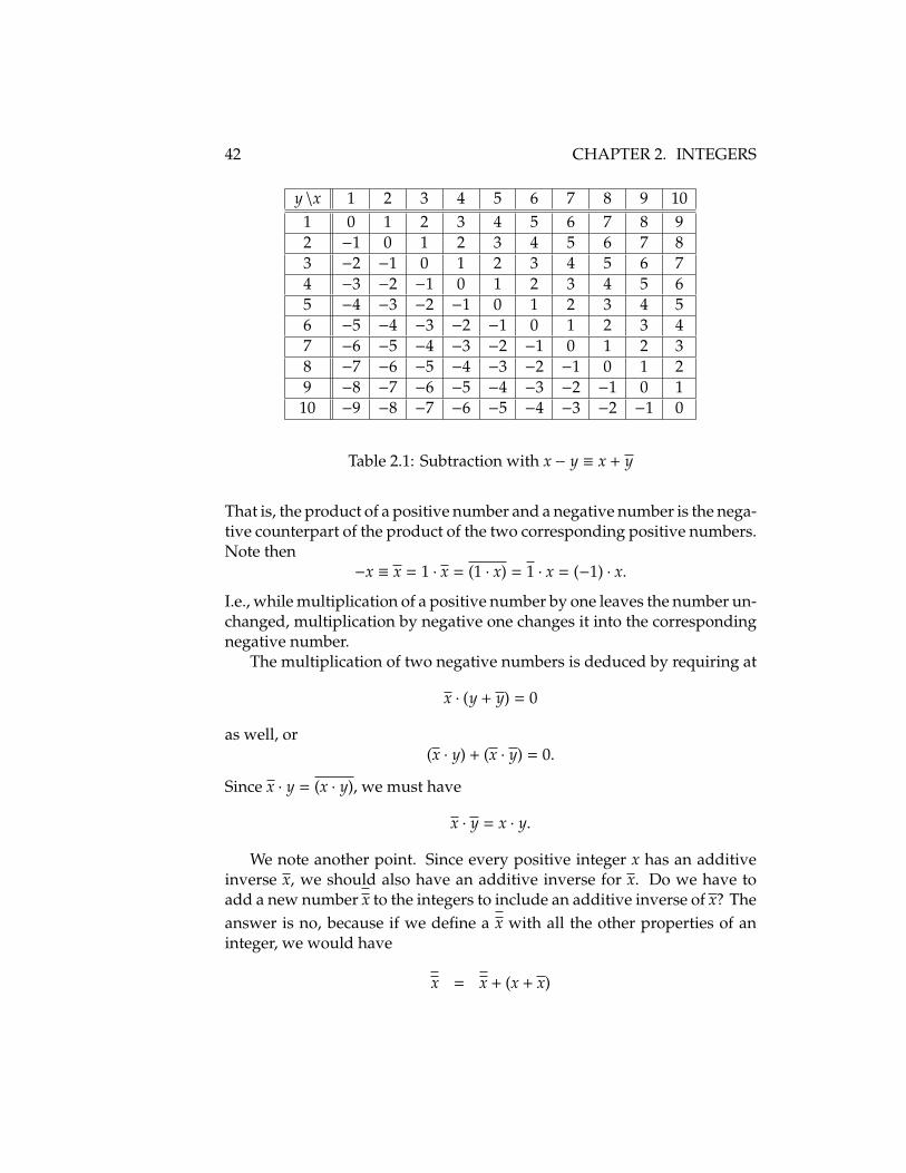
which is often used to indicate that x is positive. Table 2.1 shows thesubtraction table for the first few decimal numbers using this notation.
Similarly, we define multiplication of a positive number by a negativenumber by noting
x · (y + y) = x · 0 = 0 = (x · y) + (x · y).
Thus, since x · y + (x · y) = 0, we define
x · y = (x · y).
42 CHAPTER 2. INTEGERS
y \x 1 2 3 4 5 6 7 8 9 101 0 1 2 3 4 5 6 7 8 92 −1 0 1 2 3 4 5 6 7 83 −2 −1 0 1 2 3 4 5 6 74 −3 −2 −1 0 1 2 3 4 5 65 −4 −3 −2 −1 0 1 2 3 4 56 −5 −4 −3 −2 −1 0 1 2 3 47 −6 −5 −4 −3 −2 −1 0 1 2 38 −7 −6 −5 −4 −3 −2 −1 0 1 29 −8 −7 −6 −5 −4 −3 −2 −1 0 1
10 −9 −8 −7 −6 −5 −4 −3 −2 −1 0
Table 2.1: Subtraction with x − y ≡ x + y
That is, the product of a positive number and a negative number is the nega-tive counterpart of the product of the two corresponding positive numbers.Note then
−x ≡ x = 1 · x = (1 · x) = 1 · x = (−1) · x.I.e., while multiplication of a positive number by one leaves the number un-changed, multiplication by negative one changes it into the correspondingnegative number.
The multiplication of two negative numbers is deduced by requiring at
x · (y + y) = 0
as well, or(x · y) + (x · y) = 0.
Since x · y = (x · y), we must have
x · y = x · y.
We note another point. Since every positive integer x has an additiveinverse x, we should also have an additive inverse for x. Do we have toadd a new number x to the integers to include an additive inverse of x? Theanswer is no, because if we define a x with all the other properties of aninteger, we would have
x = x + (x + x)
2.4. AN ALTERNATE APPROACH 43
= (x + x) + x= 0 + x= x.
So, if x is the additive inverse of x, then x is the additive inverse of x.Finally, we point out some possible confusion with the notation −a
for a. This comes about because we also use “−” to denote subtraction; i.e.,x− y ≡ x+ y. If we use a negative sign in both senses in the same expression,we have to be careful about what it means. For example, consider thedistribution law. Being careful about notation tells us that
x · (y − z) = x · (y + (−z))= x · (y + z)= (x · y) + (x · z)= (x · y) + x · z= (x · y) − (x · z).
Thus the distribution law for multiplication over addition also tells us howto distribute multiplication over subtraction; it is not a separate question.
2.4 An Alternate Approach
We can derive all the results of the previous section with a very generalargument. In particular, the basic problem is to define elements to add tothe natural numbers that decrease them as well as increase them.
Suppose we look at a particular problem. We want to add an element 1to the natural numbers so that adding it to a natural number decreases it.Now, since 1′ > 1, let us define 1 to be the solution of
1′ + 1 = 1.
It turns out that the only other assumptions we need, other than that thisequation has a solution, is that 1 and all the numbers generated by multiply-ing or adding a natural number to 1 exist, and satisfy the basic propertiesof the natural numbers. In particular,
x + y = y + x,x + (y + z) = (x + y) + z,
x · y = y · x,

44 CHAPTER 2. INTEGERS
x · (y · z) = (x · y) · z,x · (y + z) = x · y + x · z,
where x, y and z are any numbers that can be formed as sums or productsof the natural numbers and 1. We also assume that 1 · x = x for any suchnew element introduced, as it does for the natural numbers.
For example, we have
1 = 1′ + 1,= (1 + 1) + 1,= 1 + (1 + 1).
Our assumption is that 1 + 1 must be a number; call it 0 (zero). Then zerohas the property
1 + 0 = 1.
Now examine a general natural numbers x. Suppose for a particular xthere exists an x such that
x + x = 0.
Clearly, this is true for x = 1, with x = 1. Then
(x + x) + 1 = 1,(x + 1) + x = 1,
x′ + (x + 1) = 1 + 1,x′ + (x + 1) = 0.
Then there exists a number x′ = x + 1 such that
x′ + x′ = 0.
Thus for any natural number x there exists an x such that x + x = 0.Next, we require that 1 · 0 be a number. Since
1 · x = x
for all natural numbers x, we assume this also holds for x = 0. Then
1 · 0 = 0.
2.5. DECIMAL SUBTRACTION 45
Now suppose x · 0 = 0 for the natural number x. We know this holds forx = 1. Then we have
x · 0 + 0 = 0 + 0,x · 0 + 1 · 0 = 0 + (1 + 1),
(x + 1) · 0 = (0 + 1) + 1,x′ · 0 = 1 + 1,x′ · 0 = 0.
Then x · 0 = 0 for all natural numbers x.Finally, we note that if there is “another zero 0” such that
x + 0 = x
for any x, we need only add x to both sides of the equation to find
x + x + 0 = x + x,0 + 0 = 0,
0 = 0,
where we have used our assumption that 0 + x = x for any x is also true forx = 0.
2.5 Decimal Subtraction
First consider binary subtraction, which (as in any number system) is equiv-alent to finding z = x+y. We have assumed that x and y are natural numbers,and that x > y, as all other cases can be reduced to this case.
As with our discussion of addition, we write the natural number z aszn . . . z1z0. Our algorithm will calculate zi given xi and yi. As with addition,it is useful to define ci, which in this case will indicate whether it wasnecessary to “borrow” from xi′ or successive digits in order to restrict zi to0 or 1.
This comes about when we realize that x+y = z means finding a numberz such that
y + z = x.
We would like to have this hold for each digit individually; i.e., we wouldlike to solve
yi + zi = xi,

46 CHAPTER 2. INTEGERS
with yi and xi given, and zi = 0 or 1. But this isn’t always possible, as wecan see if yi = 1 while xi = 0. The solution is to define wi from yi + wi = xi,and then let
wi = zi + ci′ + ci′ .
Then if yi = 1 and xi = 0 gives wi = 1, we have ci′ = 1 producing zi = 1.The 1 + 1 in the ith place become just 1 in the (i′)th calculation
xi′ + yi′ → xi′ + yi′ + 1 = (xi′ + 1) + y.
Thus instead of carrying into the next place, we are “borrowing” from xi′ .We can think of borrowing as carrying a negative number. Thus for the ith
digit, we look for solutions of the form
yi + zi + ci′ + ci′ ,= xi + ci,
The ci on the right indicates whether we have borrowed from xi to calculatethe previous digit. This gives an explicit expression for
zi = xi + ci + yi + ci′ + ci′ .
If xi + ci + yi is a negative number, we choose ci′ = 1 and carry 1 to (borrow1 from) xi′ . An explicit example is the worse case of xi = 0 with both ci andyi = 1, for then the sum of these three terms is 1 + 1. We would then chooseci′ = 1, giving zi = 0.
In explicitly writing an algorithm using Boolean expressions, it is firstuseful to determine how many bits we need to extract from xi. This isdetermined from yi and ci, and it is useful to define
τ20 = ¬yi ∧ ¬ci,
τ21 = (yi ∧ ¬ci) ∨ (¬yi ∧ ci),τ22 = yi ∧ ci
Then whether we need to borrow from xi′ depends on whether xi representsenough bits to provide the bits required. Thus
ci′ = τ22 ∨ (¬xi ∧ τ21).
Similarly,zi = (¬xi ∧ τ21) ∨ (xi ∧ (τ22 ∨ τ20)).

2.5. DECIMAL SUBTRACTION 47
We can approach decimal subtraction in the manner we first approacheddecimal addition. If
x =
nx∑
i=0
xi · 10i,
y =
ny∑
i=0
yi · 10i,
then
z = x − y =
max(nx,ny)∑
i=0
(xi − yi) · 10i
However, the terms xi − yi in general may not all be positive or negative.It is not usual to represent an integer as a string of digits that are eitherpositive or negative, but as either
z = zn . . . z1z0,
orz = −z = zn . . . z1z0 = −zn . . . z1z0.
As for addition, arranging a number is standard form is called normalizingthe number. For example, the above prescription would give
222 − 315 = 113 = 1 · 102 + 1 · 101 + 3 · 102 = −1 · 102 + 1 · 101 − 3 · 102
We first choose to make the left-most digit positive, in this case by multi-plying by −1; i.e.
222 − 315 = 113 = −113 = −(1 · 102 − 1 · 101 + 3 · 100).
Then we can make all the interior digits positive, in this case, by writing
222 − 315 = −(0 · 102 + (10 − 1) · 101 + 3 · 100). = −(9 · 101 + 3) = −93.
Note that we have “borrowed” 1 · 102 to add 10 · 101 to the −1 · 101 term.The coefficient of 101 then becomes 9, a positive number. We see that this isa general way of making the coefficient of a 10i-term a positive digit if westart from the right-most end of the number. This works because we alwayshave something to borrow from the next term on the left.
We can write down a general algorithm for calculating x − y if x , y(and neither x or y is zero) as follows.
48 CHAPTER 2. INTEGERS
1. If x > 0 and y < 0, set x − y = x + |y| and quit.
2. If x < 0 and y > 0, set x − y = |x| + y and quit.
3. Otherwise, x and y are of the same sign. Define variables r and s to bethe absolute values of x and y such that r > s. Then t = r − s > 0 andx − y = ±t. We make t > 0 so that we know to “borrow” from ti+1 inorder to make ti > 0. So either r = |x| and s = |y|, or r = |y| and s = |x|.
4. Define ti = 0 for all i, and if ri or si are not explicitly defined considerthem to be equal to zero. Define a “borrow number” bi. Set an indexi to zero, and set b0 = 0.
5. Set ti = ri + si + bi.
6. If ti < 0, define ti = ti, set ti = ti + 10, and set bi′ = 1. This is equivalentto borrowing 1 from ri′ and adding 10 to ri. Otherwise, set bi′ = 0.
7. If i < nr, i < ns, or bi′ , 0, increment i by 1 and go to 5.
8. If x > 0 and y > 0, set x− y = t if x > y, or x− y = t if x < y. Then quit.
9. If x < 0 and y < 0, set x − y = t if |x| > |y|, or x − y = t if |x| < |y|. Thenquit.
The difference between addition and subtraction of decimal integers is thatfor addition, we sometimes need to “carry” a result over to the coefficientof the next power of 10, while with subtraction we “borrow” from the nextpower of 10.
The following sequence shows successive steps in subtracting 1847 from10729. The number being subtracted is called the the subtrahend, and thenumber being subtracted from is called the minuend. The result is thedifference. The calculation is usually organized by writting the minuend onone line, the subtrahend on the next, and the difference following. Thisleads to the following sequence:
1 0 7 2 9− 1 8 4 7
2
⇒6 12
1 0 7/ 2/ 9− 1 8 4 7
8 2
⇒
16
−1 6/ 12
1 0/ 7/ 2/ 9− 1 8 4 7
8 8 2
⇒
9 16
0 −1/ 6/ 12
1/ 0/ 7/ 2/ 9− 1 8 4 7
8 8 8 2
For the right-most digit (or the first digit counting from the right), no bor-rowing is necessary. However, the next digit to the left asks for subtracting

2.5. DECIMAL SUBTRACTION 49
4 from 2. Since 4 > 2, we borrow 10 from the left, changing the 2 to a 12, andthe 7 on the left to a 6. We indicate this by writing the new subtrahend digitabove a crossed-out original digit. On the third digit, we want to subtract 8from 6, which requires borrowing from the 0 on the left. This can be doneif we note that 0 − 1 = −1, so we now have 16 in the third place. Since16 − 8 = 8, the third digit of the answer is in the acceptable range of 0 − 9.Finally, we need to borrow in the fourth place, changing the −1 to 9. Thisgives the fourth digit of the answer as 8. There is no fifth digit in the finalanswer, since the 1 in the fifth place in the minuend has been borrowed forthe fourth-place calculation.
We can also do subtraction by carrying a negative number. Here’s theprevious calculation using this method:
− 1 1 1
1 0 7 2 9− 1 8 4 7
8 8 8 2
Note that we have put a negative sign on the line indicating carries. Thisis because a 1 on this line means that the subtrahend (original secondline) should be increased (unlike addition, where either original line canbe increased) for that digit’s calculation. Furthermore, if there’s a carryassociated with the digit to the left, 10 is added to the minuend (originalfirst line). This is because we are carrying a negative number; i.e., carrying-10 to the left means that 1 is subtracted from the calculation on the leftwhile 10 is added to the current calculation. For example, focus on thethird digits, which originally is 7 − 8. We carry -10 to the left, giving 17 − 8except for the carry into the third digit from the second. This means that weshould be calculating 17−9 = 8, which is the final answer for the third digit.Negative carrying makes subtraction look similar to addition (see p. 21), butone must be careful about both adding and subtracting the carries in theappropriate manner.
We note that no special rules need be enumerated when decimal num-bers are multiplied. We use the same algorithm as for positive numbers,and note that the product is positive if the two numbers have the same sign.Otherwise, the product is negative.
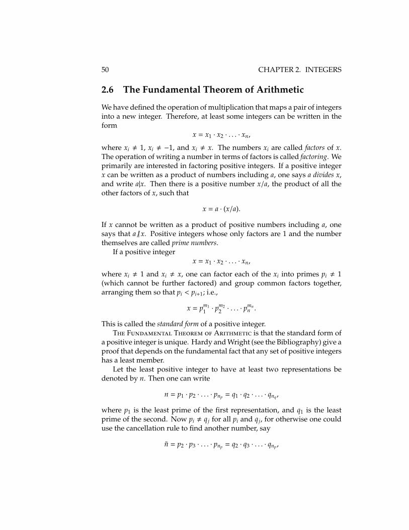
50 CHAPTER 2. INTEGERS
2.6 The Fundamental Theorem of Arithmetic
We have defined the operation of multiplication that maps a pair of integersinto a new integer. Therefore, at least some integers can be written in theform
x = x1 · x2 · . . . · xn,
where xi , 1, xi , −1, and xi , x. The numbers xi are called factors of x.The operation of writing a number in terms of factors is called factoring. Weprimarily are interested in factoring positive integers. If a positive integerx can be written as a product of numbers including a, one says a divides x,and write a|x. Then there is a positive number x/a, the product of all theother factors of x, such that
x = a · (x/a).
If x cannot be written as a product of positive numbers including a, onesays that a 6 | x. Positive integers whose only factors are 1 and the numberthemselves are called prime numbers.
If a positive integerx = x1 · x2 · . . . · xn,
where xi , 1 and xi , x, one can factor each of the xi into primes pi , 1(which cannot be further factored) and group common factors together,arranging them so that pi < pi+1; i.e.,
x = pm11 · p
m22 · . . . · p
mnn .
This is called the standard form of a positive integer.T F T A is that the standard form of
a positive integer is unique. Hardy and Wright (see the Bibliography) give aproof that depends on the fundamental fact that any set of positive integershas a least member.
Let the least positive integer to have at least two representations bedenoted by n. Then one can write
n = p1 · p2 · . . . · pnp = q1 · q2 · . . . · qnq ,
where p1 is the least prime of the first representation, and q1 is the leastprime of the second. Now pi , q j for all pi and q j, for otherwise one coulduse the cancellation rule to find another number, say
n = p2 · p3 · . . . · pnp = q2 · q3 · . . . · qnp ,
2.6. THE FUNDAMENTAL THEOREM OF ARITHMETIC 51
with n < n and with two representations, which would be a contradiction.Now consider p1 · q1. Since p1 and q1 are the smallest in their respective
factorizations, p1 · p1 ≤ n and q1 · q1 ≤ n, (“≤” is “less than or equal”). Thenp1 · q1 < n, and
N = n − p1 · q1,
is a positive number with a unique factorization. Since p1 can be written asa factor of n,
N = p1 · (p2 · . . . · pn − q1),
one has p1|N. Similarly, q1|N, so since N has a unique factorization,
N = p1 · q1 · N,
andn = p1 · q1 + N = p1 · q1 · (1 + N),
Thenq1|(n/p1)
orq1|p2 · . . . · pn.
But this is a contradiction, since n/p1 < n (and thus has a unique factoriza-tion) and q1 , pi for all pi.
To illustrate the ideas of this proof, let us suppose that we know that22 = 2 · 11, and we suspect that 22 is the minimum positive integer with adifferent factorization. Let us assume the alternate factorization involves 3.In this case, take p1 = 2, q1 = 3, and p1 · q1 = 6. Then N = n − p1 · q1 = 16would have a unique factorization involving both 2 and 3, and 3 would bea factor of 16/2 = 8. But 36 | 8. Thus N cannot have a unique factorizationinvolving both 2 and 3, and 22 cannot have one factorization involving 2and another involving 3.
We notice an interesting feature of this proof: The unique factorizationis true of the natural numbers by themselves, but we used the properties ofa number generated by subtraction,
N = n − p1 · q1
= (p1 · p2 · . . . · pn) − (p1 · q1)= (p1 · p2 · . . . · pn) + p1 · q1
= p1 · ((p2 · . . . · pn) + q1)= p1 · ((p2 · . . . · pn) − q1),

52 CHAPTER 2. INTEGERS
to prove the theorem. We haven’t developed any parallel manipulation forworking with n = N + p1 · q1, which is what one can write using naturalnumbers alone. In other words, a feature (subtraction) of a larger system(the integers) which is not available in the system of the natural numbers,is used to prove a theorem about the natural numbers, a subset of the largersystem.
2.7 Abstract Characterization of Integers
A ring is a set of objects with binary1 operations “+” (addition) and “·”(multiplication) with properties
1. Addition is commutative: a + b = b + a.
2. Addition is associative: (a + b) + c = a + (b + c).
3. There exists an element 0 such that a + 0 = a for all integers a.
4. For any integer a there exists an integer a such that a + a = 0. That is,each integer has an additive inverse.
5. Multiplication is associative: (a · b) · c = a · (b · c).
6. Multiplication distributes over addition: a · (b + c) = (a · b) + (a · c).
Integers are a commutative ring:
7. Multiplication is commutative: a · b = b · a.
Integers are a commutative ring with unity:
8. There exists an element 1 such that a · 1 = a for all integers a.
The integers have properties in addition to those of a commutative ringwith a unity. They also form an integral domain. An integral domain is acommutative ring with unity where
9. a · b = 0 implies a = 0 or b = 0.
This property by itself implies the cancellation law for multiplication. Forif c , 0 and a · c = b · c, then (a − b) · c = 0. Since c , 0, a − b = 0, or a = b.
The abstract notion of the order of two integers a and b is described bynoting whether a − b is positive or negative. An integral domain D is an
1A binary operation is a rule which produces a single output from two inputs.

2.7. ABSTRACT CHARACTERIZATION OF INTEGERS 53
ordered integral domain if there exists a subset Dp ⊂ D (a setDp whose everyelement also belongs toD), called the positive elements, such that for all aand b inDp
1. If a, b ∈ Dp, then a + b ∈ Dp.
2. If a, b ∈ Dp, then a · b ∈ Dp.
3. For all c ∈ D, either c ∈ Dp, c ∈ Dp, or c = 0.
The first two properties are called closure under addition and multiplication,respectively. The third property is called the trichotomy law. If a , b, thea + b is either in Dp (is positive) or it is not. In the former case, one writesa > b. In the later case,
a + b = a + b = b + a
is positive, and b > a.Note that since a is the additive inverse of a, if a > b we have
a + b ∈Dp, (2.1)
a + b ∈Dp, (2.2)
b + a ∈Dp, (2.3)
orb > a,
in agreement with intuition.The closure relations insure that inequalities have certain expected in-
tuitive behaviors. For example, a > b and c > 0, one expects that a + c > b.This follows from closure under addition, for a > b means a + b ∈ Dp, andc > 0 means c ∈ Dp. Then closure under addition gives
a + b + c = (a + c) + b ∈ Dp,
ora + c > b.
Similarly, closure under multiplication means that if a > b and c > 0,a c > b c. For
a + b ∈ Dp,
a c + b c ∈ Dp,
a c + b c ∈ Dp,
a c> b c.

54 CHAPTER 2. INTEGERS
One can define the absolute value |a| of an integer a by
• If a ∈ Dp, |a| = a.
• If a ∈ Dp, |a| = a.
In the later case, we can write a = 1 · |a| = −|a|. Thus |a| is always positive;i.e., belongs toDp.
The final defining property of the integers is that the positive integers arewell-ordered. We know this from the fact that we constructed the positiveintegers from the natural numbers, and we have shown that the naturalnumbers are well-ordered.
But if one assumes that the integers are an integral domain with a well-ordered subsetDp, one can show thatDp is the set of natural numbers.
First note that there can’t be any positive numbers between 0 and 1. Forsince the positive integers are well-ordered, let x be the minimum positiveinteger. Assume
0 < x < 1.
Then one would have0 < x2 < x.
But x2 is a positive integer by the closure property, so x2 < x violates thedefining property of x. Thus 1 is the minimum positive integer.
Now a setA that includes 1 and includes a + 1 if it includes a is the setof positive integers Dp. For let B be the set of all positive integers not inA. Suppose B is nonempty. It does not include 1 (the minimum positiveinteger), because 1 ∈ A by definition. Since B ⊂ Dp, it is well-orderedand has a minimum element b > 1. Then b − 1 > 0, so b − 1 ∈ A. Butb − 1 ∈ A implies (b − 1) + 1 = b ∈ A by the defining property ofA, whichis a contradiction. Thus B is empty, andA = Dp.
2.8 Constructing the Integers
We have postulated that we can create an element zero and a set of nega-tive numbers with a one-to-one correspondence with the natural numbers,and combine them with the natural numbers (now also called the positivenumbers) to create a set called the integers. We have defined addition andmultiplication between all combinations of zero, negative and positive in-tegers. It is plausible that this has been done consistently, but we haven’treally proved that in the manner that we did for the natural numbers.
2.8. CONSTRUCTING THE INTEGERS 55
For the natural numbers, we postulated that they are defined by Peano’saxioms. Then we defined addition and multiplication in terms of successors,as provided by those axioms. Then, in addition to suggestive argumentsusing a beaded string, we proved (in the Appendix to the first chapter) thatthose definitions imply that addition and multiplication are associative andcommutative, and that addition distributes over multiplication. In order toprovide the same degree of confidence in the properties of the integers, itis useful to consider the integers as a ordered pair of natural numbers. Wewrite
X = (x+, x−),
where x+ and x− are natural numbers whose properties we have alreadyestablished. Ordered means that the order of the pair matters; i.e., in general
(x+, x−) , (x−, x+).
Consideration of integers as ordered pairs is suggested by the problemof keeping a running count of some quantity that can both increase anddecrease. For example, suppose one has a herd of cattle. The herd canincrease when one buys more cattle. The herd can decrease when we sellcattle, or they are lost through predators or natural causes.
Recall that for any two natural numbers x, y, either x = y, or there existsa natural number u such that x = y + u, or there exists a natural number usuch that y = x + u. As far as the size of the herd is concerned, the totalnumber in the herd at any one time is the difference between the sum of allthe cattle we have acquired and the sum of all the cattle that we have lost. Ifwe keep track of the two sums, gains and losses, we can determine the sizeof the herd at any one time by finding the number that added to the lossesequals the gains. The point is that by maintaining two numbers using onlyaddition, we can always find the current size of the herd.
This suggests that addition of integers as an ordered pair should consistsof addition of the components; i.e.,
X + Y = (x+, x−) + (y+, y−) = (x+ + y+, x− + y−).
Furthermore, we guess that X and X differ in that their components areinterchanged; i.e.,
X + X = (x+, x−) + (x−, x+) = (x+ + x−, x− + x+).
This implies that an ordered pair with equal components should be in-terpreted as 0, and it is the difference in the components that determine

56 CHAPTER 2. INTEGERS
the corresponding natural number. So we need a way of identifying theproperties of an integer when the components are not equal.
The key point here is that, from our point of view, the only thing thatmatters is whether the first or second element of the pair is larger, and whatthe difference between them is. In other words, we really don’t care whatthe absolute size of the elements is, we just care about these two properties.
So, from our point of view, we don’t need equality of the ordered pairs,we need equivalence. Equivalence is defined by an equivalence relation. Ifwe have an equivalence relation “∼” satisfied by two quantities x and y, wewrite x ∼ y. The properties that make an equivalence relation useful are:
Reflexive Law X ∼ X.
Symmetric Law If X ∼ Y, then Y ∼ X.
Transitive Law If X ∼ Y and Y ∼ Z, then X ∼ Z.
“Equivalence” is “equal in some sense,” and we use the equal sign “=,”in this sense—as an equivalence relation. This is not the same thing as“identical.”
For example, consider different species of money. The American dollar($) was once convertible to the English pound (£) at the rate of $5 = 1£. Thiswas a time when $5 was “equal,” in the sense of purchasing power, to 1£,without being “identical.” The equivalence relation is shorthand for tellingus whether two items are the same for the purposes we are talking about.
Since for any two natural numbers x, y, either x = y, or there exists anatural number u such that x = y + u, or there exists a natural number usuch that y = x + u. we can write an integer as either (x0, x0), (x0 + x+, x0),or (x0, x0 + x−). We define the standard form of an integer as that obtainedby letting x0 = 1
Then for the integer X = (x+, x−) we can reduce X to standard form(x+, x−). where either x+ = 1 or x− = 1 or both. We define
1. X = O if x+ = 1 and x− = 1
2. X is a positive integer if x+ is a natural number and x− = 1
3. X is a negative integer if x+ = 1 and x− is a natural number.
We define X = Y as true if X and Y have the same standard form. Thiswill be true for X = (x+, x−) and Y = (y+, y−) if
x+ + y− = x− + y+,

2.8. CONSTRUCTING THE INTEGERS 57
because it holds if x+ and x− differ by the same amount as y+ and y−. Itis not affected if a single number is added to both x+ and x−, or a differentnumber added to both y+ and y−. Clearly, “=” in this sense is an equivalencerelation.
We note that
(x+, x−) + (1, 1) = (1, 1) + (x+, x−) = (x+ + 1, x− + 1) = (x+, x−),
where the last form follows by reduction to the standard form. So wehave an integer, O = (1, 1), that satisfies one of the requirements for azero, namely X + O = O + X = X. We have already noted that for anypositive integer X = (x, 1) there exists a negative integer X = (1, x) suchthat X + X = 0.
Now one sees easily that the integers are commutative and associativeunder addition:
X + Y = (x+, x−) + (y+, y−)= (x+ + y+, x− + y−)= (y+ + x+, y− + x−)= (y+, y−) + (x+, x−)= Y + X.
and
X + (Y + Z) = (x+, x−) + ((y+, y−) + (z+, z−))= (x+, x−) + (y+ + z+, y− + z−)= (x+ + (y+ + z+), x− + (y− + z−))= ((x+ + y+) + z+), (x− + y−) + z−)= ((x+ + y+), (x− + y−)) + (z+, z−)= (X + Y) + Z.
Next we note that a positive integer corresponding to the natural numberx can be chosen of the form X = (x′, 1) and a corresponding negative integerof the form X = (1, x′). Then each representation of an integer will have twocomponents that are different (since 1 is the successor of no natural number),and will have an obvious correspondence with a particular natural number(since each natural number has a unique predecessor). That is, the set ofall pairs (x′, 1) includes all the natural numbers: With x = 1, it includesan element (1′, 1) that corresponds to the natural number 1. If the pair

58 CHAPTER 2. INTEGERS
(y, 1) corresponds to the natural number x, then (y′, 1) corresponds to thenatural numbers x′. Thus by induction the set of all (x′, 1) corresponds tothe set of all natural numbers. Similarly, by induction there is an orderpair of the form (1, x′) that also corresponds to the natural numbers, but(x′, 1) , (1, x′).
With the definition of the successor of a positive integer as
X′ = (x′, 1)′ ≡ (x′′, 1),
and withI ≡ (1′, 1),
as the generalization of the natural number 1, addition of positive integerssatisfies the same definition of addition as the natural numbers, namely
X + I = (x′, 1) + (1′, 1)= (x′ + 1′, 1 + 1)= (x′ + 1 + 1, 1 + 1)= (x′′ + 1, 1 + 1)= (x′′, 1)= X′,
andX + Y′ = X + (Y + I) = (X + Y) + I = (X + Y)′.
The later property follows from the associativity of integers.Multiplication is defined by
(x+, x−) · (y+, y−)≡(x+ · y+ + x− · y−, x+ · y− + x− · y+).
This form is motivated by noting that we suspect that each term in theproduct (as for natural numbers themselves) is a sum of products of twonatural numbers, one from a component of each integer. In order to satisfythe postulated rules on multiplication of positive and negative integers, theproduct must be positive if both terms come from the positive parts of eachinteger or from the negative parts of each integers. It must be negative ifone term comes from the positive part and one from the negative part of aninteger.
One can also write
(x0 + x+, x0 + x−) · (y0 + y+, y0 + y−) =
(z0 + x+ · y+ + x− · y−, z0 + x+ · y− + x− · y+),
2.8. CONSTRUCTING THE INTEGERS 59
wherez0 = x0 · (y0 + y+ + y−) + (x0 + x+ + x−) · y0.
Thus as with addition, multiplication of X and Y can be carried out with anyrepresentation of X or Y as long as it is equal to the corresponding standardrepresentation.
We notice that
X ·O = (x+, x−) · (1, 1) = (x+ + x−, x+ + x−) = (1, 1) = O,
so the second requirement for zero is met.Using x · y′ = x · y + x for the natural numbers, we explicitly verify that
the multiplicative properties of I = (1′, 1) hold:
X · I = (x+, x−) · (1′, 1)= (x+ · 1′ + x− · 1, x+ · 1 + x− · 1′)= (x+ · 1 + x+ + x− · 1, x+ · 1 + x− · 1 + x−)= ((x+ + x−) + x+, (x+ + x−) + x−)= (x+, x−)= X.
We note that the multiplication rule gives X ·Y = X ·Y, so that Y = I ·Y = I ·Y.As we have seen for addition, because we can regroup the natural
numbers as necessary when we actually carry out multiplication, we alsohave X · Y = Y · X, and
(X · Y) · Z = ((x+ · y+ + x− · y−) · z+ + (x+ · y− + x− · y+) · z−,(x+ · y+ + x− · y−) · z− + (x+ · y− + x− · y+) · z+)
= ((x+ · (y+ · z+ + y− · z−) + x− · (y+ · z− + y− · z+),(x+ · (y+ · z− + y− · z+) + x− · (y+ · z+ + y− · z−))
= X · (Y · Z).
We also have the distribution law:
X · (Y + Z) = (x+ · (y+ + z+) + x− · (y− + z−),x+ · (y− + z−) + x− · (y+ + z+))
= ((x+ · y+ + x− · y−) + (x+ · z+ + x− · z−),(x+ · y− + x− · y+) + (x+ · z− + x− · z+))
= (X · Y) + (X · Z).

60 CHAPTER 2. INTEGERS
The distribution law, along with X · I = X, allows us to show that thedefinition of multiplication holds for integers as it does for the naturalnumbers:
X · Y′ = X · (Y + I) = X · Y + X · I = X · Y + X.
The fact that we can define a subset {Xi = (x′i , 1)} of the integers, definea successor X′i = (x′′i , 1) to Xi also in the subset while satisfying Peano’s ax-ioms, and show that the set of Xi satisfy the defining equations for additionand multiplication of the natural numbers, shows that the natural numberscan be considered a subset of the integers.
2.9 Summary
The integers are a well-ordered integral domain. A well-ordered integraldomain is an ordered integral domain where any nonempty subset of thepositive elements has a least element.
An ordered integral domain is an integral domain with a subset calledthe positive elements that is closed with respect to addition and multiplica-tion, and such that any element is either a positive element, or its additiveinverse is a positive element, or it is the element zero.
An integral domain is a commutative ring with unity such that thecancellation law for multiplication holds. A commutative ring with unityis a commutative ring with an element whose product with each element ofthe ring is that element. A commutative ring is a ring where multiplicationis commutative.
A ring is a set of element with the operations of addition and multi-plication, where addition is associative and commutative, multiplication isassociative, addition distributes over multiplication, there exists an elementzero that when added to any element gives that element, and for each ele-ment of the ring there exists another element which when added to it giveszero.
From these properties, it has been demonstrated that a subset of the in-tegers that includes the unity element, and has the property that an elementbelonging to the set implies the element added to unity also belongs to theset, then that subset includes all the positive integers.
We have show that a system with these properties can be constructedfrom the natural numbers. This system consists of an ordered pair of naturalnumbers. If the first number of the pair is greater than the second, the pairrepresents a positive integer. If the second number of the pair is greater

2.10. APPENDIX 61
than the first, the pair represents the additive inverse of a positive number.If the two numbers of the pair are equal, it represents the zero.
2.10 Appendix
We have already shown, through the explicit construction of the integersas an ordered pair of natural numbers, that zero can be included in the setof integers. It is also possible to integrate zero into the system of naturalnumbers by defining the first symbol of Peano’s axioms to be zero insteadof one. Zero becomes the element which is the successor of no element, andthe seccessor of zero is defined to be one; i.e.,
0′ = 1.
Then addition is defined by
x + 0 = x,x + y′ = (x + y).′
Note that this defines the successor of any number to be one plus the numberin a slightly different manner than did the first scheme, for now we have
x + 0′ = (x + 0)′,x + 1 = x′.
since x + 0 = x, instead of x + 1 = x′ directly as before. Then the secondequation defining addition has the same effect as it did under the originalset of Peano’s axioms.
The extension to multiplication with zero is
x · 0 = 0,x · y′ = (x · y) + x.
Then choosing y = 0 in the second equation give
x · 1 = x · 0 + x,
orx · 1 = x,
as expected.
62 CHAPTER 2. INTEGERS
Now we show that addition and multiplication including zero eachsatisfy associativity and commutativity, and that multiplication distributesover addition. Recall from the Appendix of the first chapter that theseproperties were shown by proving that they hold for one of the variablesset to one in an equation, and that induction implies the equation hold forits successor as well. So inclusion of zero involves showing that the relationholds for one of the variables set to zero; then the equation for succeedingnumbers holds by induction.
Associativity of Addition. To start from zero, we only need to note that
(x + y) + 0 = x + y = x + (y + 0).
Commutativity of Addition. Similarly, to include zero in commmutativitywe need to show that
x + 0 = 0 + x,
for all x. This holds for x = 0, so look at
x′ + 0 = x′
= (x + 0)′
= (0 + x)′
= 0 + x′.
if x + 0 = 0 + x.
Distribution Law. To carry through the proof for the distribution law, weonly need to show that
x · (y + z) = (x · y) + (x · z),
for z = 0. But
x · (y + 0) = (x · y) = (x · y) + 0 = (x · y) + (x · 0).
As before, we can now use induction to show the case holds when z is notzero.
Multiplication Lemma. To prove x′ · y = (x · y) + y by induction, we needto show that this holds when y = 0. But
x′ · y = x′ · 0 = 0,
2.10. APPENDIX 63
and(x · y) + y = (x · 0) + 0 = 0 + 0 = 0.
so one can proceed as before to the case of a general y through induction.
Commutativity of Multiplication. To use induction to prove commutativ-ity of multiplication, we need to show that 0 · y = y · 0 for all y. Clearly, thisholds for y = 0. Then
0 · y′ = (0 · y) + 0 = 0 · y,
andy′ · 0 = (y · 0) + 0.
Thus if 0 · y = y · 0, then 0 · y′ = y′ · 0. We can then use induction on x = 0as before.
Associativity of Multiplication. Note that
(x · y) · 0 = 0,
andx · (y · 0) = x · 0 = 0.
Thus (x · y) · z = x · (y · z) for z = 0. Then as in the previous chapter, one thencan use induction to show that the relation holds for z in general.

64 CHAPTER 2. INTEGERS
Chapter 3
Rational Numbers
Earlier, we have seen that it has proven useful to augment the naturalnumbers with zero and the negative numbers. We did this by introducing,for each natural number x, a corresponding negative number x such that
x + x = 0,
where 0 (zero) is a number such that
x + 0 = x,x · 0 = 0.
We think of zero as a place holder that represents “nothing”, as in “addingnothing to a number gives the same number back,” and negative numbersare the additive inverses of the positive numbers.
Just as the addition of zero and negative numbers allows us to extendour ability to keep track of the size of a group of objects by allowing the sizeto decrease as well as increase, it is useful to extend the idea of counting toinclude objects that don’t come in whole units.
For example, consider two herds of cattle. One herd consists of largeanimals, the other of small. Suppose that we want to “count” the cattle interms of some standard weight, say, that of a standard rock, rather than asindividual animals. Then we can more realistically compare the relativeworth of the two herds. We can easily split the standard rock into halves,those halves in halves (giving a quarter rock), and so forth. Then one animalmight weight the same as 10 rocks, one half rock, and one eighth rock. Aneighth rock, for example, would be what you would get splitting a quarterrock in half.
65

66 CHAPTER 3. RATIONAL NUMBERS
One might think of this as a generalization of counting by extendingcounting to measuring. We are measuring the weight of the herd, rather thancounting the number of cattle. It turns out possible to do this by addingmultiplicative inverses to the set of integers to form the rational numbers.
3.1 Multiplicative Inverses
For each nonzero integer x (positive or negative) we introduce a numbercall the multiplicative inverse, written x−1, defined by the property
x · x−1 = 1.
The notation x−1 comes from
xu+v = xu · xv,
and the observation that
1 = x0 = x1+1 = x1−1 = x1 · x−1 = x · x−1.
The practical significance of the multiplicative inverse is seen if wegeneralize our idea of the natural numbers as a string of beads. Rather thana string of beads, just think of a straight line marked at regular intervals.The interval between zero and one represents a certain length. Then sincex ·x−1 = 1, and multiplying something by x gives x copies of that something,it is reasonable to think of x−1 as the xth fraction, or part, of the intervalbetween zero and one.
For example, the animal in our example that weighted the same as 20rocks, a half rock and an eighth rock would be described as weighing thesame as 20 + 2−1 + 8−1 rocks.
Since the zeroth part of something is zero, one might suspect that therecan’t be anything that can be multiplied by zero to give one. This is correct.For since
x · 0 = 0 = y · 0,giving zero a multiplicative inverse would imply
x · (0 · 0−1) = y · (0 · 0−1),
(assuming associativity of multiplication by 0−1) leading to
x · 1 = y · 1,

3.2. ORDER AND MULTIPLICATIVE INVERSES 67
orx = y
for all x and y. Basically, multiplication by zero removes all informationabout what has been multiplied. That information cannot be recovered.One just does without a multiplicative inverse of zero.
We also note in passing that zero is the only number that is its ownadditive inverse. For if there is another number with the defining propertyof 0, we would have
0 + 0 = 0.
But0 + 0 = 0 + 0 = 0
by the property of zero itself, so
0 = 0.
So in that sense zero is unusual even with respect to addition.
3.2 Order and Multiplicative Inverses
If a and b are positive integers with a > b, define a−1 and b−1 to be positive.Recall that a > b means
a + b > 0.
Then multiplying by a−1 · b−1 and assuming a−1 and b−1 have all the usualassociativity and commutativity properties of integers, we have
(a−1 · b−1) · a + (a−1 · b−1) · b> 0,
(b−1 · a−1) · a + a−1 · (b−1 · b)> 0,
b−1 · (a−1 · a) + a−1 · (b−1 · b)> 0,b−1 + a−1 · (b−1 · b)> 0,
b−1 + a−1 > 0.b−1 > a−1.
In particular a−1 < 1 if a > 1.Thus, when multiplicative inverses are added to the integers, there are
at least as many rational numbers between zero and one as there are positiveintegers. This has the important result that while the rational numbers areordered, they are no longer well-ordered. That is, there are sets of rational

68 CHAPTER 3. RATIONAL NUMBERS
numbers bounded below that do not have a least element. An example isthe set of all multiplicative inverses greater than zero. For suppose x−1
min isthe lease multiplicative inverse greater than zero. Then xmin is an integer,and xmin + 1 is an integer greater than xmin. Then (xmin + 1)−1 < x−1
min, whichcontradicts the assumption the x−1
min is the desired least element.
3.3 Operations with Multiplicative Inverses
We first note that1 · 1 = 1,
so that1−1 = 1.
More generally,(x−1)−1 = x.
That is, the multiplicative inverse of the multiplicative inverse of a numberis the number itself. This follows from
(x−1)−1 = (x−1)−1 · (x · x−1),
=((x−1)−1 · x−1
)· x,
= x,
where we have assumed that x−1 has all the commutative, associative anddistributive properties that the integers have.
From the interpretation of the multiplicative inverse and the fact thatwe want to treat it as a number like the positive and negative integers, it isclear we should define
(x · y)−1 ≡ y−1 · x−1.
Then we have
(x · y) · (x · y)−1 = (x · y) · (y−1 · x−1)= ((x · y) · y−1) · x−1
= (x · (y · y−1) · x−1
= (x · 1) · x−1
= x · x−1,
= 1.
3.4. FRACTIONS 69
Addition of multiplicative inverses is a bit more complicated. We firstnote that
x−1 = x−1 · (y · y−1) = y · (x · y)−1,
which is easily interpreted as y times the (x · y)th part of one. It is clear howto add different multiples of the (x · y)th part of one. So we write
x−1 + y−1 = x−1 · (y · y−1) + y−1 · (x · x−1)= y · (x−1 · y−1) + x · (x−1 · y−1)= (x + y) · (x · y)−1,
to definex−1 + y−1 ≡ (x + y) · x−1 · y−1.
3.4 Fractions
It is common notation to write
x · y−1 =xy.
Then
x−1 = 1 · x−1 =1x.
and
x ·(1x
)= 1.
When one writes x−1 as 1x (or commonly 1/x), we speak of 1
x as a fraction.Since x ·
(1x
)= 1, one can think of 1
x as something that when added tox copies of itself is equivalent to 1. This gives an interpretation of x
y as xcopies of something of which it takes y copies to add up to one. The obviousexample is “half” a cake or half a pie, written 1/2, where the 1 indicates thatwe’re referring to that partition of the cake (or pie) into pieces that require 2such pieces to make a whole cake (or pie). A corollary to that interpretationis that
xy
=w xw y
,
since x copies of something that takes y copies to add up to one is the sameas w x copies of something that takes w y copies to add to up one. For

70 CHAPTER 3. RATIONAL NUMBERS
example, 24 of a pie is the same as 1
2 of a pie. This also follows from ourformal rules above by
xy
= x · y−1 = x · y−1 · w · w−1 = w · x · w−1 · y−1 =w xw y
.
Multiplying in or cancelling out a common factor in the two parts of afraction is a common technique in manipulating fractions.
We also call x/y a fraction, where x is called the numerator of the fraction,and y is called the denominator. The multiplication of x by the multiplicativeinverse of y, which is what x/y means, is also called dividing x by y. Theact of dividing is called division, and is often given the symbol “÷”. Thusx/y is often written x ÷ y. The result of a division is called the quotient, asin the quotient of x ÷ y is z. Thus we have division as multiplication bythe multiplicative inverse, in a manner analogous to defining subtractionas addition of the additive inverse.
Our rules for combining fractions then are:
1(1x
) = x,
(1x
)·(
1y
)=
1(x · y)
,
(1x
)+
(1y
)=
(x + y)(x · y)
.
It is also clear we should have(
xy
)·(u
v
)= x ·
(1y
)· u ·
(1v
)= x · u ·
(1y
)·(1v
)=
(x · u)(y · v)
.
To illustrate manipulations with fractions, consider(
xy
)+
(uv
)=
(xy
)·(vv
)+
(uv
)·(
yy
)
=
((x · v)(y · v)
)+
((u · y)(v · y)
)
=((x · v) + (u · y))
(y · v),
where the basic strategy is to multiply numerators and denominators ofthe various components until the denominators are all the same. Then one
3.4. FRACTIONS 71
can add the numerators. One usually dispenses with all the parenthesisby saying all the terms in the numerator are evaluated separately, as areall the terms in the denominator. In both numerator and denominator,multiplication has precedence over addition, and each fraction is evaluatedindependently before being combined with another. Then
xy
+uv
=x · v + u · y
y · v .
A slightly more subtle example is division of fractions, as in
abcd.
This is written out as
ab·( cd
)−1= a · b−1 ·
(c · d−1
)−1
= a · b−1 · c−1 ·(d−1
)−1
= a · b−1 · c−1 · d,
orabcd. =
ab· d
c
This justifies the oft-used prescription for dividing fractions; namely, invertthe denominator (i.e., exchange the numerator and denominator in thebottom fraction), then multiply that fraction by the original numeratorfraction. This is sometimes shortened to “invert and multiply.”
Another justification of “invert and multiply” follows from
abcd
=a db dc bd b
=a db c
=ad· c
d.
Here we have successively multipied the numerator and denominator offractions by the same factor, and finally cancelled the common factor of(d b)−1 in the fraction involved in the last step.
In some practical applications of these formulas, it is useful to note
z =z1,
72 CHAPTER 3. RATIONAL NUMBERS
so, for example,xy
+ z =xy
+z1.
Then one can apply the general formula to write
xy
+ z =x + y · z
y.
A common shorthand is to write
z +xy
= zxy,
where the addition symbol is understood.Lastly, we note that the additive inverse of a fraction follows from
(xy
)= x · y−1 = x · y−1 =
xy,
since (xy
)+
xy
= (x + x) · y−1 = 0.
Of course, this is not the only way of writing it, because we could use
(xy
)=
xy,
just as well.These results mean that there is often a lot of implicit notation involved
in calculations with fractions. For example, suppose one has 1 12 baskets of
apples and sells 34 a basket. How much is left? We have
112− 3
4= 1 +
12
+(34
)
=11
+12
+34
=22
+12
+34
=32
+34
=64
+34

3.5. DECIMAL FRACTIONS 73
=6 + 3
4
=34.
3.5 Decimal Fractions
We have represented positive decimal integers as
x =
n∑
i=0
xi · 10i.
With multiplicative inverses, we can represent numbers that involve in-verses of powers of 10. In which case, it is usual to sum the terms bystarting with the largest. Thus we write
x =
n∑
i=0
xm−i · 10m−i.
where n can be greater than m.To see that such numbers exist, recall that
10 · 10−1 = 1 = 101 · 10−1 = 101−1 = 100.
Indeed, this is why we have defined x0 = 1, x1 = x, and use the notation x−1
for the multiplicative inverse of x. Then any number of 10’s and (10−1)’swill satisfy
10−m · 10n = 10n−m,
(m, n > 1) after 10−1 · 101-pairs are combined as ones.So there are fractions that can be written in the form
y =x
10k
=
∑ni=0 xn−i · 10n−i
10k
= 10−kn∑
i=0
xn−i · 10n−i
=
n∑
i=0
xn−i · 10n−k−i
74 CHAPTER 3. RATIONAL NUMBERS
=
n∑
i=0
xm+k−i · 10m−i
=
n∑
i=0
ym−i · 10m−i,
where we have defined yi = xi+k and m = n− k. If m = n, we have our usualrepresentation of a decimal natural number. We note that since a nonzeroxi represents a contribution to the magnitude of x greater than any possiblesum of terms with x j, j < i, the same is true for the yi multiplying possible10i < 1 in the representation of y.
One can expand the usual representation, whether binary or decimal, ofan integer to include rationals, where m > n, by using a period to separatethe coefficients of 100 = 1 and 10−1 (for decimals), as in
2.37 ≡ 2 · 100 + 3 · 10−1 + 7 · 10−2.
The period in a decimal rational number is called the decimal point, and theradix point for systems like the binary system that are based on a differentradix.
Addition of decimal rationals is consistent with this notation, as we canwrite
2.1 + 1 = 10−1 · 21 + 1= 10−1 · (21 + 10)= 10−1 · 31= 3.1 .
Multiplication is even simpler—
2.3 · 4.1 = (10−1 · 23) · (10−1 · 41)= 10−2 · 23 · 41= 10−2 · 943= 9.43 .
3.6 Division for Positional Systems
Let us consider division in a positional number system. In addition tomultiplying an integer by a multiplicative inverse, divsion often refer to

3.6. DIVISION FOR POSITIONAL SYSTEMS 75
the mechanical process of finding the representation of a rational number.When determining the representation of
z =xy,
x is called the dividend and y is called the divisor.The simplest such system we consider is the binary system, and the
problem we wish to solve is to find a positional representation of a fraction
xy
=
n∑
i=0
zm−i · 2m−i.
We note that while m in general will be fixed and either positive or negative,n may be limited either by the desired accuracy in the result, or by thepossibility that no finite n will satisfy this requirement exactly.
We start by writing this relationship in the form
x = y ·n∑
i=0
zm−i · 2m−i.
Since 2m represents the largest contribution to z, m is determined by therequirement
y · 2m+1 > x ≥ y · 2m.
Recall that 2m will be larger than the contributions of the remaining terms inz. If m is smaller than required, not even the sum of the remaining terms hasthe potential to make the required contribution. If m is larger than required,z will be too large, and the remaining terms only add more contributions.
The next nonzero contribution is determined by
y · 2m−i+1 > x − y · 2m ≥ y · 2m−i.
That is, we just subtract the known contribution to z, and add a term tolessen the difference between x and the known terms, assuming that thisdifference is greater than zero. In general, then we will have
y · 2m−i+1 > x − y ·i−1∑
j=0
zm− j · 2m− j ≥ y · 2m−i,
where zi is either 0 or 1. At any step, if the difference between x and a sumof finite terms in y · z gives zero, we are finished, since no additional termsare necessary to satisfy x = y · z.

76 CHAPTER 3. RATIONAL NUMBERS
For example, consider 2/5 in binary form. We have 2 = 10 and 5 = 101.Then the first term is determined by
101 · 2m+1 > 10 ≥ 101 · 2m.
If m = −2, we have101 · .1 > 10 ≥ 101 · .01,
or10.1 > 10 ≥ 1.01
So m = −2. To get the next term, note that
x − y · 2−2 = 10 − 101 · .01 = 10 − 1.01 = .11.
So we need1.01 · 2−i+1 > .11 ≥ 1.01 · 2−i,
or i = 1. Thus the first two terms of 2/5 in the binary representation give
10101
= .011 + . . .
This is illustrated in Fig. 3.1.
.01100. . . quotient101)10.00000. . . divisor ) divident
1 01110 x − y · 2−2
101100. . . x − y ·∑1
i=0 z−2−i · 2−2−i
Fig. 3.1 - Classic Binary Long Division
Note that when we get to the last printed line of Fig. 3.1, we are calculat-ing 1
101 . This is a repeat of the first part of the calculation. This means thatthe pattern we have generated so far will just be repeated over and overagain. Thus we find
10101
= .01100110011 . . . .
Division of decimals is done in the same basic manner, although weneed to determine a digit that is not just zero or nonzero. We can illustrate

3.6. DIVISION FOR POSITIONAL SYSTEMS 77
the calculation somewhat differently by repeatedly writing the numeratorof a fraction as some multiple of the denominator, plus a remainder. As in
25
=20 · 10−1
5
=205· 10−1
=4 · 5
5· 10−1
= 4 · 10−1
= .4 .
This is just a somewhat more verbose expression of the basic algorithmillustrated in Fig. 3.1, but in a decimal representation. In this case in thedecimal system there is no remainder. A more complicated example is
2.15
=21 · 10−1
5
=215· 10−1
=4 · 5 + 1
5· 10−1
= 4 · 10−1 +15· 10−1
= 4 · 10−1 +105· 10−2
= 4 · 10−1 + 2 · 10−2
= .42 .
As with our binary calculation, the process may not terminate; e.g.,
23
=203· 10−1
=18 + 2
3· 10−1
=(6 +
23
)· 10−1.
The remainder 23 · 10−1 is just 10−1 times the original fraction, so we see that
the remainder will factor in the same way as the first term. In other words,the process will continue indefinitely, and we write
23
= .6666 . . . .

78 CHAPTER 3. RATIONAL NUMBERS
But remember that 10−n is something that when multiplied by 10n gives one.If one corresponds to the interval between zero and one when the integersare arranged along a line, 10−n represents a shorter and shorter interval as ngets larger. Then the interval represented by the difference between .66 and.666 is 10 times smaller than the interval between .6 and .66. Thus there isusually a practical limit to the required number of digits to the right of thedecimal pointed needed to represent a decimal number.
We conclude by noting that the multiplicative inverse x−1 of x is just 13 .
Thus, for example
3−1 =13
= .33333 . . . .
We can write down a general algorithm for decimal division by notingthat if q is a rational number q = x
y with x and y integers, we want
q =xy
=
n∑
i=0
qm−i · 10m−i,
with qm−i being decimal digits between 0 and 9. This can be arranged bybeginning with m and qm chosen with a two-step process. First choose msuch that
y · 10m+1 > x ≥ y · 10m
Then choose qm by requiring that
y · (qm + 1) · 10m > x ≥ y · qm · 10m
with qm a decimal digit. This second step is an extra step that is not requiredfor a binary calculation, because qm can only be 1 in that case.
Next choose qm−i by a similar two-step approach. First choose i suchthat
y · 10m−i+1 > x − y ·i−1∑
j=0
qm− j · 10m− j ≥ y · 10m−i
Then choose the decimal digit qm−i by requiring
y · (qm−i + 1) · 10m−i > x − y ·i−1∑
j=0
qm− j · 10m− j ≥ y · qm−i · 10m−i
For the rational numbers q = xy , this can be formalized as follows:
1. Choose n to be the number of digits desired in the representation.

3.6. DIVISION FOR POSITIONAL SYSTEMS 79
4.552)234.0
20826 026 0
0
Fig. 3.2 - Classic Long Division
2. Choose m such that y · 10m+1 > x ≥ y · 10m.
3. Choose a decimal digit qm such that y · (qm + 1) · 10m > x ≥ y · qm · 10m.
4. Set the remainder R = x − y · qm · 10m.
5. Choose i such that y · 10m−i+1 > R ≥ y · 10m−i.
6. Choose qm−i such that y · (qm−i + 1) · 10m−i > R ≥ y · qm−i · 10m−i.
7. Set R = R and R = R − y · qm−i · 10m−i. If R = 0, you are done.
8. If i + 1 < n, increment i and go to item 5.
If n > 0 and n > m, the result has the decimal form
Q = qmqm−1 . . . q0 . q−1 . . . qm−n,
(the decimal point is between q0 and q−1) with remainder R, so that q =Q + R. The remainder may be dropped and Q modified if the answer isrounded. That is, one may choose qm−n according to whether incrementingqm−n lessens the difference between Q and q. For example, suppose x
y =
3.2 + .06, where Q = 3.2 and R = .06. Then 3.3 is a better approximationto 3.26 than 3.2 is, and one would round x
y to 3.3. Whether one rounds ifR = .05 would be a matter of convention, since rounding or not roundinggives a representation of x
y to the same accuracy.Fig. 3.2 shows an example of the use of this algorithm in the form of the
classical decimal long division procedure. This algorithm makes especiallyeffective use of the positional characteristic of the decimal representation ofnumbers; i.e., that the coefficient of 10i is in the ith place from the left side ofthe number (counting i = 0 as the first place). Here we illustrate the divisionof 23.4 by 5.2, or 23.4 ÷ 5.2. One places the numerator under the division
80 CHAPTER 3. RATIONAL NUMBERS
symbol ) , and the denominator to the left. Both the numerator and thedenominator are multiplied by powers of ten so that the denominator is theminimum possible positive integer. The location of the decimal point in thenumerator will also be the location of the decimal number of the quotient.
Then m and qm are determined by the requirement above, and the prod-uct of the denominator with qm is placed below the numerator. In addition,qm is place above the division symbol. Both these numbers are placed sotheir least significant digit aligns with the least significant digit of the partof the numerator they are chosen to match. The product of the denominatorand qm is then subtracted from the numerator. The result of this subtractionis then matched with the next digit of the quotient. If the quotient is zero,the process terminates exactly; otherwise the process is carried out as far asdesired.
3.7 Abstract Characterization of Rationals
A field is a commutative ring with an identity in which each element a , 0has a multiplicative inverse a−1 such that a · a−1 = 1. The rationals aretherefore a field.
A field is an integral domain, for if a · b = 0 and a , 0, then (a−1 · a) · b =1 ·b = b = 0. Similarly, if b , 0, one shows a = 0 by multiplying the equationby b−1.
One notes that if a > 0, a−1 > 0. Similarly, since the product of twonegative numbers is positive,
(−|a|)−1 = −|a|−1.
That is, the multiplicative inverse of a negative number is negative.Since the multiplicative inverse of positive numbers is positive and unity
is positive, the rational numbers are still ordered; i.e., the positive rationalsare closed under addition and multiplication, and a rational number a iseither a positive number, zero, or its additive inverse is a positive number.However, the rational numbers are no longer well-ordered.
Consider the setA of all elements greater than some positive element a.If b were the least element ofA, consider c = (a + b) · 2−1. Since b > a,
c > (a + a) · 2−1 = 2 · a · 2−1 = a,
and c ∈ A. Butc < (b + b) · 2−1 = 2 · b · 2−1 = b,

3.8. CONSTRUCTING THE RATIONALS 81
which contradicts the assumption b is the least element ofA. Thus,A hasno least element.
Similarly, one can always find a rational number between any two ra-tional numbers.
3.8 Constructing the Rationals
As with the integers, it is convenient to consider the rationals as an orderedpair, but in this case we consider them to be an ordered pair of integers ratherthan natural numbers. The first number of the pair can be considered to bethe numerator of a fraction, and the second number can be considered tobe the denominator; e.g.,
X = (xn, xd).
Then if x is an integer, the rational number it corresponds to is
X = (x, 1).
The rational number corresponding to x−1 is
X−1 = (1, x).
Multiplication is defined by
X · Y = (xn · yn, xd · yd).
We first note that if X = (x, 1) corresponds to the integer x, and Y = (y, 1)corresponds to the integer y, then X ·Y = (x · y, 1 · 1) = (x · y, 1) correspondsto the integer x · y, as expected.
Again, it is clear thatX · Y = Y · X,
and
X · (Y · Z) = (xn · yn · zn, xd · yd · zd)= (X · Y) · Z.
We note thata · a−1 = (a, 1) · (1, a) = I,
and that(xn, yd) · I = (xn, yd) · (a, a) = (xn · a, xd · a).
82 CHAPTER 3. RATIONAL NUMBERS
Since both pairs represent the same rational number, we extend the notionof “equal” so that
X = Y
ifxn · yd = xd · yn.
Thus a common factor in xn and xd doesn’t affect whether X = Y. while westill have X = Y if xn = yn and xd = yd.
Next, addition is defined as
X + Y = (xn · yd + xd · yn, xd · yd).
Again, we note that if X corresponds to the integer x, and Y corresponds tothe integer y, then X + Y = (x · 1 + 1 · y, 1 · 1) = (x + y, 1) corresponds to theinteger x + y,
It is clear thatX + Y = Y + X,
and
X + (Y + Z) = (xn, xd) + (yn · zd + yd · zn, yd · zd)= (xn · yd · zd + xd · yn · zd + xd · yd · zn, xd · yd · zd)= (xn · yd + xd · yn, xd · yd) + (zn, zd)= (X + Y) + Z.
We also have the distribution law:
X · (Y + Z) = (xn(·yn · zd) + xn(·yd · zn), xd · (yd · zd))= (xn · yn, xd · yd) + (xn · zn, xd · zd)= X · Y + X · Z.
3.9 Summary
We have extended the well-ordered integral domain of integers to the fieldof rationals by the addition of a multiplicative inverse of each integer exceptzero.

3.9. SUMMARY 83
We have shown how fractions are another representation of rationalnumbers. We have shown how to represent rationals in the decimal num-ber system, and how to perform addition and multiplication of decimalnumbers
We have seen that the rationals are still ordered, but no longer well-ordered.
We have shown that a field with these properties can be constructedfrom the integers by considering a rational number to be an ordered pair ofintegers.

84 CHAPTER 3. RATIONAL NUMBERS
Chapter 4
Real Numbers
It turns out that rational numbers are incomplete, in the sense that there aresequences of rational numbers whose successive values increase monoton-ically (xm+1 ≥ xm) and are bounded above, but do not converge to a limitthat is a rational number. This unexpected shortcoming is remedied withthe irrational numbers, which, together with the rational numbers, make upthe real number system.
4.1 Sequences
From the decimal representation of a rational number,
x = 10−mm+n∑
i=0
xi · 10i,
and the fact that 10−i can be interpreted as one 10i-th the interval betweenzero and one when the integers are marked off along a line, one realizesthat the term involving 10−i makes a smaller and smaller contribution to xas i increases. One suspects that the sequence {xm} defined by
xm = 10−mm+n∑
i=0
xi · 10i,
would converge on a specific number as m increases, as long as 0 ≤ xi < 10.We have already seen sequences that do converge, simply because x−i =
0 for i greater than a specific number. An example is x = .42. But we have
85
86 CHAPTER 4. REAL NUMBERS
also seen sequences that do not terminate; e.g.,
(1/3)1 = .3,(1/3)2 = .33(1/3)3 = .333
. . .
Yet in this case it seems obvious (1/3)m → (1/3) (“→” reads “approaches”)as m→∞ (m increases without limit).
For x = 3, let us calculate how much xm differs from 1/3 by writing
x = xm + εm.
In this case, we have
εm = (1/3) − xm,
3 · εm = 1 − 3 · xm.
But3 · xm = . 99 . . .︸︷︷︸
m times
,
so
εm =10−m
3.
As we suspect, the error in xm decreases rapidly with increasing m.We note that xm+1 = xm + δm, where both xm and δm are rational; e.g.,
.33 =3
10+
3100
=30 + 3
100=
33100
,
etc. So we have a monotonically increasing (xm+1 > xm) infinite (no limitto the number of elements in the sequence) sequence of rational numbersbounded above (εm > 0, so xm < 1/3) apparently converging to a definiterational number. If the rational numbers can represent anything that wecan think of as a “number.”, one would think that any such monotonicallyincreasing sequence bounded above would converge to a rational number.
In fact, it is not hard to find a monotonically increasing sequence bound-ed above that can be shown not to converge to a rational number. Consider

4.1. SEQUENCES 87
the sequence {xm} where xm is the largest rational number involving termsequal or larger than 10−m whose square is less than 2. One finds
x0 = 1,x1 = 1.4,x2 = 1.41,x3 = 1.414,...
with
(x0)2 = 1,(x1)2 = 1.96,(x2)2 = 1.9881,(x3)2 = 1.999396,
... .
The sequence is monotonically increasing, and is clearly bounded above by,say, x = 2. It would appear to be converging, as we see by writing
x = xm + εm,
x2 = (xm + εm)2,
2 = x2m + 2 · xm · εm + ε2
m,
2> x2m + 2 · xm · εm,
εm <2 − x2
m
2 · xm.
The error decreases as (xm)2 gets closer to 2, and we are causing (xm)2 to getcloser to 2 by a factor of 10 each iteration.
But the problem is that a number whose square is 2 cannot be representedas a rational number, so the series is not converging to a number in the setof rational numbers. This is a consequence of the fundamental theorem ofarithmetic, which says that there is only one way to factor a number. Thussuppose that it was possible to represent the square root of 2 (written
√2)
as a rational number. One would have√
2 =x1 · x2 · . . . · xm
y1 · y2 · . . . · yn,

88 CHAPTER 4. REAL NUMBERS
where xi , y j for all i, j. Multiplying by the denominator and squaring, onewould have
2 · y21 · y2
2 · . . . · y2n = x2
1 · x22 · . . . · x2
m.
But since there is only one way to factor either side of this equation, eitherthe left hand side has 1 or an odd number of 2’s in it, and the right had sidehas 0 or an even number of 2’s in it. This is a contradiction, so
√2 cannot
be represented as a rational number.
4.2 Irrational Numbers
The problem of infinite1 sequences bounded above that appear to convergeto a number not in the rationals is remedied by adding elements to the setof rationals.
Dedekind2 realized that a monotonically increasing sequence boundedabove divides the rationals into two sets: The set of rationals L less thanor equal to any member of the sequence, and the set of rationalsU greaterthan any member of the sequence. The key point is thatU may or may nothave a least element. This partition of the rationals defines a cut.
For example, for the sequence (1/3)m discussed earlier, the number 1/3 isgreater than any xm, and therefore is an upper bound of the sequence. And1/3 is a least upper bound. For if we assume x < 1/3 is an upper bound,let δ = (1/3) − x. But the difference between 1/3 and xm is εm = 10−m/3,for which an m can be chosen so that εm < δ. So there is a xm > x, whichcontradicts the assumption that x is an upper bound.
However, if we define a cut using the sequence xm with x2m < 2 discussed
earlier, the sequence has no rational least upper bound. For assume that xis a least upper bound. Let δ = x2 − 2 > 0 (not = 0, since there is no rationalnumber whose square is 2) and x = x − (δ/2). Then x2 = x2 − δ + (δ2/4) =2 + (δ2/4) > 2. Then x < x is also an upper bound in U, contradicting anassumption that x is the least upper bound.
Dedekind generalized the idea of a rational number by defining the realnumber system to include all the rational numbers plus all the numbersneeded so that any such cut included a least element in U. If the leastelement inU is not rational, it is said to be irrational.
1Clearly, monotonically increasing finite sequences of rational numbers always convergein a trivial sense. Similarly, if all the sequences made from subsets of strictly increasingelements xm+1 > x are finite, the sequence always converges.
2See the bibliography.
4.3. APPLICATIONS 89
Thus in the real number system, a monotonically increasing sequencebounded above always defines a sequence converging on a particular x.Because with the least element x in U for any monotonically increasingsequence {xm} and any δ, one can always find an integer n such that
xm + δm = x,
with δm < δ for all m > n, no matter how small δ is.3 For suppose no suchn can be found. That would imply that x − δ/2 < x belongs toU because itis greater than any xm. But x is the least upper bound, so this would be acontradiction.
The property of the real number system that for any set of reals withan upper bound, there is a least upper bound (not necessarily in the set), iscalled completeness.
Irrational numbers were introduced with the idea of filling in “holes”in the rationals; i.e., we intend to fill in the holes between the rationalnumbers when we complete them to form the reals. On reflection, wemight wonder whether, by defining numbers as upper limits of boundedinfinite sequences, we might have somehow introduced irrational numbersin some place other than the holes between rationals. For example, have weintroduced irrational numbers that are larger than any rational number?
We have not, because of the A P of the reals. TheArchimedean Property states that for any real number x there is an integern ≥ x. For let Sx be the set of all integers less than or equal to x. Then Sxis bounded above by x, and hence there is a real number x that is the leastupper bound of Sx.4 Since x is a least upper bound to Sx, there is a integerm ∈ Sx such that m > x − 1 (otherwise x − 1 would be an upper bound).Then m + 1 > x, and so is not in Sx. But m + 1 is also an integer, so Sx cannotinclude all the integers. So x cannot be greater than all integers.
4.3 Applications
Nth Root of a Positive Real number. The existence of a least upper boundfor a monotonically increasing bounded set of numbers allows us to showthat there exists a real number x > 1 satisfying
y = xn,
3This is what one means by convergence.4Note that we have not used the fact that that x is an integer. All that is required is that
Sx have a least upper bound in the reals. Of course, all integers are also reals.

90 CHAPTER 4. REAL NUMBERS
for all y > 1, where n is an integer greater than 1.To show this, construct the sequence of numbers x−m such that
(x−m)n ≤ y < (x+m)n,
withx+
m = x−m + αm,
where αm is α raised to the mth power and α < 1. The previous exampleof constructing an approximation to y = x2 corresponds to the case y = 2,n = 2, and α = .1.
Since y > 1, we have yn > y, and y is an upper limit on x−m. Then theset {x−m} has a least upper bound, which we will call x−. Similarly, x+
m hasa greatest lower bound, which we will call x+. We will show x− = x+ = x.For either x+ − x− = ε, x+ − x− = −ε, or x+ − x− = 0, with ε > 0. Supposex+ − x− = ε > 0. Since
x+ − x− ≤ x+m − x−m = αm.
x+ − x− can be made smaller than ε, giving a contradiction. The onlypossibility is x+ = x− = x.
Next we need to showy = xn.
Now either y − xn = 0, y − xn = ε, or y − xn = −ε, where ε > 0. Supposey− xn = ε. Then since y < (x+
m)n by construction, and x ≥ x−m because x = x−
is a least upper bound, we have y− xn < (x+m)n − (x−m)n. If y− xn < 0, writing
xn − y > 0 and using x+m > x+ = x with y > (x−m)n allows one to write
|y − xn| < (x+m)n − (x−m)n,
for all three possibilitiesUsing the identity
an − bn = (a − b) · (an−1 + an−2 b + an−3 b2 + . . . + bn−1),
we have
(x+m)n − (x−m)n = (x+
m − x−m) ·((x+
m)n−1 + (x+m)n−2 x−m + (x+
m)n−3 (x−m)2 + . . . + (x+m)n−1
),
or(x+
m)n − (x−m)n < (x+m − x−m) n (x+
m)n.
4.3. APPLICATIONS 91
This gives(x+
m)n − (x−m)n < n (x+m)n αm,
which can be made as small as desired. So the assumption |y − xn| = ε > 0leads to a contractions if m is large enough. Thus y − xn = 0.
Since
y = y1 = y
n times︷︸︸︷1n + 1
n +··· =
n times︷ ︸︸ ︷y
1n · y 1
n · . . . =(y
1n)n
= xn,
we are justified in writing
x = y1n ≡ n√
y.
Raising a Real Number to a Real Power. The existence of real numberssuch as n
√y means that it is possible to define raising a positive real number
to any real power. This is useful because many phenomena can be describedby a number raised to the appropriate power.
For example, consider a herd of animals. Each year, a certain fraction αof the animals produce young. Let Ny0 be the number of animals at year y0.Assume, for simpicity, that the animals give birth only once a year. Thenone would expect the number the next year to be Ny0+1 = Ny0 · (1 +α), sincethe new population is the old population Ny0 plus the births α · Ny0 . Aftertwo years, one expects
Ny0+2 = Ny0+1 · (1 + α) = Ny0 · (1 + α)2.
In general, one expects to find
Ny0+n = Ny0 · (1 + α)n.
after n years, assuming no deaths.Now in this case, we have been assuming that n is an integer. However,
we can also make a prediction for partial years, if we assume that the birthsoccur evenly throughout the year. Namely, let t be time measure in years;then one expects
N(t) = N(t0) · (1 + α)t−t0 ,
if (1 + α)t−t0 can be made to be a proper generalization of (1 + α)n. That is,we want a generalization N(t)/N(t0) = (1 + x)t−t0 of Nn/Nn0 = (1 + x)n−n0 ,where t is a real number instead of an integer like n. The general problemis to define y = xw, where w is real.

92 CHAPTER 4. REAL NUMBERS
For the moment, let us assume that the power itself is positive, as it isin the example. For a power represented as a rational number; i.e., y = xa/b,we have show one can define the bth root of x as x
1b . Then
xab =
(x
1b)a,
has the expected interpretation of the bth root of x raised to the ath power.For example, consider
232 =
(2
12)3
=(√
2)3.
We know that1.414. <
√2 < 1.415.
Cubing this, we get2.827 < 2
32 < 2.833.
If the exponent is irrational, then we can define a monotonically increas-ing sequence of rational approximations to it, again, in a manner similarto the way we defined a monotonically increasing sequence for
√2. For
example, considery = xw,
where w is irrational. If w−m < w−m+1 < w, then y−m = xw−m is a monotoni-cally increasing sequence bounded above by xwR , where wR is any rationalnumber greater than w. Let j and k be integers, and write
w−m =jmkm ,
w+m =
jm + 1km ,
where w−m ≤ w < w+m. Let
y−m = xw−m ,
y+m = xw+
m .
For example, if w =√
2, k = 10, and m = 2, then jm = 141 and y−m = xw−m =x141/100, y+
m = xw+m = x142/100.
Then y+m > 1 is monotonically decreasing (and bounded below by some
number y+) because it is a number measured in units of x1/km, which get
smaller as m increases. We can then write∣∣∣y+ − xw
∣∣∣ ≤∣∣∣y+
m − xw−m∣∣∣ =
∣∣∣xw+m − xw−m
∣∣∣ = xw−m ·(x
1km − 1
).

4.3. APPLICATIONS 93
One can show that x1/km − 1 can be made arbitrarily small by writing
x − 1 =(x
1km
)km
− 1 > km(x
1km − 1
),
where we have again used
an − bn = (a − b) · (an−1 + an−2 b + an−3 b2 + . . . + bn−1).
Thenx
1km − 1 <
x − 1km ,
and ∣∣∣y+ − xw∣∣∣ < xw−m x − 1
km .
Since xw−m is bounded and 1/km can be made arbitrarily small, we are justifiedin writing y+ = y = xw.
This is an example of a general procedure: Suppose we have a functionf (xr) defined for rational xr. Suppose that for x−1 < x < x+
1 , f (x) increases as xincreases. To define f (x) for irrational x, let x−m be a monotonically increasingsequence of rational numbers satisfying x−m < x with least upper bound x−.Similarly, let x+
m be a monotonically decreasing sequence of rational numberssatisfying x+
m > x with greatest lower bound x+. Require x−m < x < x+m with
limm→∞(x+m − x−m) = 0 (x+
m approaches x−m as m increases without limit). Ourexamples showed ways of doing this, and imply x = x− = x+. Then thereexists a number y− that is a least upper bound on y−m = f (x−m), and a numbery+ that is a greatest lower bound on y+
m = f (x+m). Now either y+ − y− = ε for
some ε > 0, or y+−y− = 0. If y+m−y−m = f (x+
m)− f (x−m) can be made as small asdesired, the only possibility is y+ = y−. We define f (x) = y+ = y− = y. Theimportant point is that y exists in the real number system. Even if all the xmare rational, the corresponding y need not be rational (as neither does x).
We have assumed that the number being raised to a power is itselfpositive. This is because if it is negative, whether the result makes sensedepends on the number. For example, since (−1)3 = −1, we can write−1 = (−1)1/3. However, there is no real number whose square is−1, so thereis no real (−1)1/2.
If the exponent is negative, we write
x−|w| =1
x|w|,
as noted before for integer w. As in that case, this is so
x|w| · x−|w| = x|w|−|w| = x0 = 1,
as desired for multiplying powers of a number.
94 CHAPTER 4. REAL NUMBERS
4.4 Constructing the Reals
We have seen that a rational number x defines a partition of the rationalnumbers into two sets: The set L of all numbers ` < x, and the setU of allnumbers u ≥ x. Furthermore, it is possible to define partitions that seem asif they “should” include a number x that has the property that any numberless than x is in L, and any number greater than x is in U, even though itcan be shown that no such number exists in the rationals. This is the casefor the partition defined by those numbers whose square is less than 2. Thatis, if there were a number x =
√2 in the rationals, any number less than
√2
would be in L, and any number greater than√
2 would be inU.Notice that partitions by themselves have properties suggestive of num-
bers. For example, partitions can be looked at in a manner that suggeststhe order property. In particular, ifL1 corresponds to one partition, andL2another, and if any x1 ∈ L1 also belongs to L2, while not all x2 ∈ L2 belongto L1, it isn’t hard to think that L1 < L2.
Furthermore, it’s possible to think of adding partitions in such a mannerthat the sum has properties similar to the sum of rational numbers. First,for a partition it is natural to associate L, rather than U, with a number,since then a larger number is associated with a larger set. Next, if x1 ∈ L1and x2 ∈ L2, then it seems reasonable to defineL = L1 +L2 as the set of allx such that there is an x1 ∈ L1 and an x2 ∈ L2 that satisfies x = x1 + x2. Thensuccessively adding, say, the partition defined by 1, we can build up largerand larger sets in a manner similar to adding 1 to the natural numbers. Wewould also expect this definition of addition to satisfy the usual propertiesof addition; e.g.,L1 +L2 = L2 +L1, and (L1 +L2) +L3 = L1 + (L2 +L3). Inthis manner, we can add the partition that separates the real numbers intothose whose squares are less than or greater than 2 to any other partition.
This suggests that it might be possible to construct a set that behaveslike an “augmented” set of rationals by considering the set of all possiblepartitions, in particular, the set of all possibleL’s, to be numbers themselves.This is in fact possible, as we are about to demonstrate. The advantage ofactually constructing the reals from the rationals is that we then know thatthe completeness property is consistent with all the properties already heldby the rationals; i.e., we can add the least upper bound of any monotonicallyincreasing bound set to the reals without upsetting any other postulate of therationals. To do this, we need to define equality, addition and multiplicationfor these sets and show that these operations satisfy the same properties forcuts as equality, addition and multiplication satisfy for the rationals.
If we are going to do operations on sets, we first need to decide how we

4.4. CONSTRUCTING THE REALS 95
know two sets are equal. If the sets are finite, then the answer is simple:Two sets are equal if they include the same elements. If the sets are infinite,we can’t always compare the sets element by element. The method usedthen for, say, two setsA and B, is to show that if a ∈ A implies a ∈ B, andb ∈ B implies b ∈ A, thenA = B. Another way to state the same idea is tosay thatA = B ifA ⊆ B (A is a subset of B with the possibility that everyelement of B is also inA) and B ⊆ A.
So we are going to construct the real number system from entire subsetsof rational numbers, namely cuts. First we formalize the definition of cuts.Following a method similar to that used by McCoy,5 we consider a cut tobe a subsetA ⊂ R+ of the positive rationals6 with the follow properties.
1. A is a nonempty subset of R+. In particular, defineA to be the subsetof R+ that does not include rationals inA. ThenA is not empty.
2. If a ∈ R+ and b ∈ R+, then a ∈ A with b < a implies b ∈ A.
3. If a ∈ A, there exists a c ∈ A with c > a. This gives a specific choiceforA if the cut defines a point in the rationals; that point is defined tobe inA.
For example, the cut Rx is defined to be the set Rx ∈ R+ such that a ∈ Rximplies a < x; i.e., Rx is the cut defined by the positive rational number x.Note that Rx and Rx are nonempty. Note that if a ∈ Rx, then a < x, so thatb < a implies b < x and b ∈ Rx. Finally, if a ∈ Rx, then there is a rationalnumber δ such that a + δ = x. Then c = a + δ/2 < x, so that c > a and c ∈ Rx.
Addition of Cuts As suggested earlier, addition of cuts is defined in theobvious way: IfA and B are cuts, thenA+B is the set of all a + b such thata ∈ A and b ∈ B. Checking,
1. Note that A + B is nonempty. Furthermore, A and B are nonempty,with elements a ∈ A and b ∈ B that are not inA +B. SoA +B is notempty.
2. If c < a + b, let x = c/(a + b). Let b = x · b. Then b < b and b ∈ B.Similarly, let a = x · a. Then a < a and a ∈ A. Then a + b = c impliesc ∈ A +B.
5See the bibliography.6McCoy considers cuts to be subsets of the entire set of rationals.
96 CHAPTER 4. REAL NUMBERS
3. SinceA andB are cuts, a ∈ A implies there exists a δa such that a+δa ∈A; and b ∈ B implies a δb with b + δb ∈ B. Then for c = a + b ∈ A +B,there exists a c + δc = a + δa + b + δb > a + b with c + δc ∈ A +B.
We note, as an observation, that if a ∈ A, then a ∈ (A+B). For choose aδ > 0 so that a + δ = a with a ∈ A, and δ ∈ B. One can always do this sinceB is not empty. Then a + δ ∈ (A +B) for all a ∈ A.
Now clearly if we want cuts to be a generalization of the positive ratio-nals, we need addition to satisfy
Rx + Ry = Rx+y.
We know that Rx + Ry defines some cut, but we need to show that it is thesame cut as that defined by Rx+y. One shows that two setsA and B are thesame by showingA ⊆ B and B ⊆ A.
1. If x ∈ Rx, x < x and if y ∈ Ry, y < y. Then x + y < x + y, x + y ∈ Rx+y,and Rx + Ry ⊆ Rx+y.
2. Similarly, if c ∈ Rx+y, c < x + y. Define w = c/(x + y). Then x = w ·x < xand x ∈ Rx. Also y = w · y < y and y ∈ Ry. Then since x + y = c,Rx+y ⊆ Rx + Ry.
Thus Rx + Ry = Rx+y.It is also clear that cuts satisfy the commutative and associative laws,
since the rational elements in the cuts satisfy those laws. ThusA+B = B+Abecause if a ∈ A and b ∈ B, a+b = b+a. Similarly, if c ∈ C, (a+b)+c = a+(b+c)implies (A +B) + C = A + (B + C).
Another property addition of cuts satisfies in common with the rationalsis thatA , A+B. To see this, choose δ small enough that δ ∈ A and δ ∈ B.Then there will be an integer n such that n · δ ∈ A but (n + 1) · δ ∈ A.However, (n + 1) · δ ∈ (A +B). So (A +B) , A.
Order Let A, B be cuts such thatA ⊂ B. Let C be the set c ∈ R+ such thatfor all a ∈ A, a + c < b for some b ∈ B. Then C is a cut, since
1. C and C are nonempty. For ifA ⊂ B, there exists a b ∈ B that is not inA. For b, there exists a δ such that b + δ ∈ B. For any a ∈ A, a < b, sothat a + δ < b + δ with b + δ ∈ B. Thus δ ∈ C. Similarly, there exits ab ∈ B so a + b < B for any a ∈ A. Thus b ∈ C.
2. If c ∈ C, for any a ∈ A, a + c ∈ B. Then for any a < a, a + c ∈ B.
4.4. CONSTRUCTING THE REALS 97
3. For all a ∈ A and any c ∈ C, there exists a b ∈ B satisfying a+c < b. Butfor each b ∈ B, there exists a δ such that b + δ ∈ B. Since a + (c + δ) <b + δ ∈ B, c + δ ∈ C.
For any two cuts A, B, it is clear either A ⊂ B, B ⊂ A, or A = B. IfA , B, there exists a cut C such that eitherA+C = B or B+C = A. To seethis, consider the caseA ⊂ B. Let C be the cut found above such that for alla ∈ A and all c ∈ C, a + c < b for some b ∈ B.
1. If a ∈ A and c ∈ C, then a + c ∈ B because a + c ∈ B for all a ∈ A bydefinition. SoA + C ⊆ B.
2. Now fix b ∈ B.
(a) If there exists an a ∈ A greater than b, find some c ∈ Cwith c < b.Then find a < a such that b = a + c.
(b) For b > a for all a ∈ A, there exists a δ such that b + δ ∈ B.Let δ = δ/3. If δ is to large to be in A, keep dividing it untilδ ∈ A. Then there will be some integer na such that na · δ ∈ Aand (na + 1) · δ ∈ A. Let a = na · δ. Then a is within δ of beinglarger than any a ∈ A. Similarly, let C ⊂ C be the set of all c suchthat a + c < b + δ for all a ∈ A. There will be some integer nc suchthat nc · δ < c for all c ∈ C, while (nc + 1) · δ > c for some c ∈ C. Letc = nc · δ. Then c is within δ of some c ∈ C. Now by constructiona ∈ A and c ∈ C. And a + c will be no more than 2 · δ less thanb + δ ≥ b + 3 · δ; i.e., b + δ > a + c > b. Let w = b/(a + c). Thenb = w · a + w · c, where w · a ∈ A and w · c ∈ C ⊂ C.
So B ⊆ A + C.
Then if there are cuts A and B with A ⊂ B, there exists a cut C such thatA + C = B.
As a consequence, ifA+C = B+C, thenA = B. For, ifA , B, supposeA = B +D. Then we would have (B +D) + C = B + C, or E = E +D withE = B + C. But this contradicts the previous result thatA , A +B.
Completeness With the ideas of addition and order defined for cuts, onecan consider the idea of completeness. Recall that completeness means thatany set of elements bounded above has a least upper bound.
For cuts, this means that for any collection of cuts M bounded above,there is a cut Slub, (possibly not in M) such that if A ∈ M, then A ≤ Slub.

98 CHAPTER 4. REAL NUMBERS
And if there exits another cut S , Slub such thatA ≤ S for allA ∈M, thenSlub < S.
Define Slub as the union of all A ∈ M. The union of two sets is the setof all the elements of both sets. Since the elements in M are sets of rationalnumbers, the union of all A ∈ M is a set of all rational numbers in any oftheA ∈M. Then
1. Slub is not empty. Furthermore, since M is bounded above, there isan element m ∈ R+ that is greater than any element in Slub. Then Slubis not empty.
2. If s ∈ Slub, then s ∈ A for some A ∈ M. Then for any b ∈ R+ withb < s, b ∈ A and b ∈ Slub.
3. If s ∈ Slub, then s ∈ A for someA ∈M. Then there exists a δ such thats + δ ∈ A, and s + δ ∈ Slub.
ThereforeSlub is a cut. Clearly, it is an upper bound for M, forSlub containsany rational number in any element of M.
Note that if S , Slub is another upper bound of M, then any rationalnumber s inS but not inSlub must be greater than any a in anyA belongingto M. But Slub consists only of a in some A ∈ M. Therefore Slub ⊂ S andSlub is the least upper bound of M.
Multiplication of Cuts Like addition, multiplication of cuts is also definedin the obvious way: IfA and B are cuts, thenA ·B is the set of all a · b suchthat a ∈ A and b ∈ B. Then,
1. We haveA·B is nonempty. Furthermore, if a ∈ A and b ∈ B, a ·b > a ·bfor any a ∈ A and b ∈ B. SoA · B is not empty.
2. If c < a · b, then c/a < b and (c/a) ∈ B. Then c = a · (c/a) ∈ A · B.
3. If a ∈ A, there exits a δ such that a + δ ∈ A. Then for c = a · b ∈ A · B,(a + δ) · b = c + δ = c ∈ A · B, with c < c.
We also want multiplication to satisfy
Rx · Ry = Rx·y.
where Rw is the cut corresponding to the positive rational number w.
1. If x ∈ Rx, x < x and if y ∈ Ry, y < y. Then x · y < x · y, x · y ∈ Rx·y, andRx · Ry ⊆ Rx·y.
4.4. CONSTRUCTING THE REALS 99
2. Similarly, if z ∈ Rx·y, z < x · y. Find a w such that z < w < x · y. Thenx = w/y < x and x ∈ Rx. Since z/w < 1, y = (z/w) · y < y and y ∈ Ry.Then x · y ∈ Rx · Ry. Since x · y = (w/y) · ((z/w) · y) = z, Rx·y ⊆ Rx · Ry.
Thus Rx · Ry = Rx·y.Therefore, we have shown that Rx · R1 = Rx, It would be useful to know
thatA · R1 = A for any cutA.
1. Clearly, if a ∈ A, and b ∈ R1, then b < 1 andA · R1 ⊆ A.
2. If a ∈ A, then there exists an a > a such that a ∈ A, and b = a/a < 1such that b ∈ R1. Then a · b ∈ A, andA ⊆ A · R1.
Thus we have shownA·R1 = A. This is the abstract property of the number1, so we define I ≡ R1.
Again, analogous to the case for the addition of cuts, it is clear that cutssatisfy the commutative and associative laws for multiplication, since therational elements in the cuts satisfy those laws. ThusA ·B = B ·A becauseif a ∈ A and b ∈ B, a · b = b · a. Similarly, if c ∈ C, (a · b) · c = a · (b · c) implies(A · B) · C = A · (B · C).
Multiplicative Inverse If A represents a rational number, then A wouldhave a least upper bound alub that would be that rational number. Thenone would expect the set B representing the multiplicative inverse of Awould be the set of all b < 1/alub. In general, we can’t assume thatA has aleast upper bound, but we do notice that if it exists, alub is inA, rather thanA. And 1/alub would be the largest number of the form 1/a with a ∈ A.But there are any number of a ∈ A arbitrarily close to alub, if it exists. Thissuggests we require that if b ∈ B there exist some a ∈ A such that b < 1/a,rather than the more specific requirement b < 1/alub.
That is, letA be a cut. LetB be the set of all b ∈ R+ such that there existsan a ∈ A with b < 1/a. Then B is a cut, since
1. B is nonempty. For if a ∈ A, 1/(2 · a) < 1/a and 1/(2 · a) ∈ B. If a ∈ A,then 1/a > 1/a for all a ∈ A. Therefore, 1/a is not in B, and B is notempty.
2. b < b with b < 1/a implies b < 1/a and b ∈ B.
3. For b ∈ B, there exists an a ∈ A such that b < 1/a. Then there exists ab with b < b < 1/a, because a rational number can be found betweenany two rational numbers. Then b < 1/a implies b < b ∈ B.
100 CHAPTER 4. REAL NUMBERS
One can verify thatA · B = I.
1. If b ∈ B, then there is an a ∈ A such that b < 1/a. Then a·b < a·(1/a) < 1for all a ∈ A, soA · B ⊆ I.
2. To show I ⊆ A · B, we need to show that for any α < 1 we can findan a ∈ A, a b ∈ B such that a · b = α, and an a ∈ A such that 1/a > b.
Note that for any a ∈ A one can write
a = α · a + (1 − α) · a>α · a + (1 − α) · a∗,
where a∗ is any element ofA. This suggests defining
δ = (1 − α) · a∗,
and noting that since δ ∈ A, there exists an integer n > 0 such thatn · δ ∈ A and (n + 1) · δ ∈ A. Let a = n · δ and a = (n + 1) · δ. Then
a>α · a + δ
> α · a + a − a,
or
0>α · a − a,a>α · a,1a>αa.
Define b = α/a. Then 1/a > b, with a ∈ A and a · b = α, as required.Then b ∈ B.
Since a ∈ A and b ∈ B, we have I ⊆ A · B.
So I = A · B.
Distributive Law We would also like to know if cuts satisfy the distributivelawA · (B + C) = (A · B) + (A · C).
1. For any r ∈ A · (B + C), we have r = a · s, with a ∈ A and s ∈ B + C.For any s ∈ B + C, we have s = b + c, with b ∈ B and c ∈ C. Thena · (b + c) ∈ A · (B + C). But a · b ∈ A · B, and a · c ∈ A · C. ThenA · (B + C) ⊆ (A · B) + (A · C).

4.4. CONSTRUCTING THE REALS 101
2. There exists an element in A · B, of the form a · b. Similarly, thereexists an element inA · C, of the form a · c. Suppose that a < a. Thena ·b+ a ·c < a · (b+c). But a · (b+c) ∈ A· (B+C), so a ·b+ a ·c ∈ A· (B+C).Thus (A · B) + (A · C) ⊆ A · (B + C).
ThenA · (B + C) = (A · B) + (A · C).We can use the distribution and trichotomy laws to show that A · C =
B · C implies A = B. For suppose A = B + D. Then we would have(B · C) + (D · C) = B · C. But this contradicts the earlier result X , X +Y.ThusA = B.
Additive Inverses We have seen that cuts in the positive rationals form aset that contains a subset that can be identified with the positive rationalsthemselves. Cuts can be given operations of addition and multiplicationthat can be identified with addition and multiplication of the positive ratio-nals, and addition and multiplication of cuts corresponding to the positiverationals produce cuts that are identified with the corresponding positiverationals. One of the cuts, I, can be identified with the special number 1.
Since the set of cuts of the positive rational numbers also contains ele-ments that do not correspond to the positive rationals, the set of cuts canbe thought of as an extension of the set of positive rationals. We have al-ready seen how to extend the set of natural numbers to include an additiveinverse. We can do likewise with cuts.
Let x be the ordered pair (X+, X−), of cuts X+ and X−. Since for anytwo cuts X+ and X−, either X+ = X−, or there exits a cut U such thatX+ = X− +U, orX− = X+ +U. Just as with the natural numbers, we definethe addition of order pairs x and y by
x + y = (X+ +Y+, X− +Y−),
and multiplication by
x · y = (X+ · Y+ +X− · Y−, X+ · Y− +X− · Y+).
We say two ordered pairs are equal if
X+ +Y− = X− +Y+,
and define the special ordered pair
1 = (I + I, I).

102 CHAPTER 4. REAL NUMBERS
Then ordered pair corresponding to the natural number x is
x = (Rx + I, I) = (Rx+1, I).
Analogous to integers, we have
x + y = (Rx+1 + Ry+1, I + I) = (Rx+y+2, R2) = (Rx+y+1, I),
as expected. Another example is
x · 1 = (Rx+1, I) · (R2, I)= (R2·x+2 + I, Rx+1 + R2),= (R2·x+3, Rx+3),= (R2·x+1, Rx+1),= (Rx+1, I),= x.
Thus as with the integers, for each x there corresponds an x such that
x + x = 0,
where0 = (I, I),
and
x + 0 = x,x · 0 = 0.
4.5 Summary
The real number system is made up of rational and irrational numbers.Like the rational numbers, the real numbers form an ordered field. The realnumber system has the additional property, not shared with the rationals,that any set of real numbers bounded above has a least upper bound (thoughthe least upper bound is not necessarily in that set, but rather in the reals).Similarly, any set of real numbers bounded below has a greatest lowerbound. This property is called completeness.
We have show that the real numbers can be build from sets of rationalnumbers. The particular sets are Dedekind cuts. A Dedekind cut is apartition of the rational number into two nonempty subsets, A and its
4.5. SUMMARY 103
complement, such that if a ∈ A and b < a, then b ∈ A; and if a ∈ A, thereexists a c > a with c ∈ A. IfA has a least upper bound a, the cut correspondsto the rational number a. Otherwise, the cut defines an irrational number.
Since there is no rational number whose square is 2, but one can definea cut using numbers whose square is less than 2, there is a real numberwhose square is 2. Since the real numbers include the rational numbers asa subset, the set of real numbers is larger than the set of rational numbers.
The existence of roots of real numbers allows one to define a real numberraised to real power.

104 CHAPTER 4. REAL NUMBERS

Chapter 5
Complex Numbers
Earlier, we have discussed the notion of a number raised to a power. Simi-larly, the notion of the nth root of a number has been introduced by notingthat there are numbers which when multiplied by themselves n times yieldthe first. An example of this is the square root of a number, as in y = x2. Inthis case, one may write x =
√y, or x = y1/2. The later notation is consistent
with the power law xa · xb = xa+b.In order for the square root of a number to exist for all positive numbers,
it was necessary to include the irrational numbers to expand rational num-bers to the set of all real numbers. In this chapter, we consider an extensionof the real numbers to the complex number system, so that even negativenumbers have a square root. As in previous expansions of various numbersystems, the complex numbers will include the reals as a subset.
5.1 The Square Root of Negative One
Since the product of two numbers, positive or negative, is always positive,there is no real number whose square is −1. So one expands the idea ofnumbers to include one with this property. Let i be defined by
i2 = −1.
We note that if real numbers can multiply i in the usual way, we get thesquare root of any negative number; e.g.,
(√
2 i) · (√
2 i) = 2 · i2 = −2.
105

106 CHAPTER 5. COMPLEX NUMBERS
This suggest that we define complex numbers as a real number plus amultiple of i; i.e.,
z = x + y i.
5.2 Addition and Multiplication
The obvious strategy is to define addition and multiplication as if i satisfiedthe usual properties of a real number, but replace i2 by −1 when it occurs.Then, for example,
z1 + z2 = (x1 + y1 i) + (x2 + y2 i)= (x1 + x2) + (y1 + y2) i.
and
z1 · z2 = (x1 + y1 i) · (x2 + y2 i)= x1 · x2 + x1 · y2 i + y1 · x2 i + y1 · y2 i2
= (x1 · x2 − y1 · y2) + (x1 · y2 + y1 · x2) i.
It is easy to verify that addition and multiplication are commutative andassociative, and that multiplication distributes over addition.
We note that0 = 0 + 0 i,
and1 = 1 + 0 i
have the properties of 0 and 1 for the reals; namely
z + 0 = z,
andz · 1 = z.
We note that there is the analogue to a magnitude or absolute value ofa complex number in
|z| =√
x2 + y2,
in that |z| = 0 if and only if z = 0. If one associates with each complexnumber z = x + y i a complex conjugate z∗ = x − y i, one sees
|z|2 = z∗ · z.

5.2. ADDITION AND MULTIPLICATION 107
The complex conjugate leads to the multiplicative inverse
z−1 =x − y ix2 + y2 =
z∗
|z|2 =z∗
z∗ · z .
The additive inverse is clearly
z = x + y i = −x − y i,
and satisfiesz = −1 · z.
One can get some feel for what addition and multiplication of complexnumbers mean by writing
z = |z|(x + y i),
wherex2 + y2 = 1.
Thenz1 + z2 = (|z1| x1 + |z2| x2) + (|z1| y1 + |z2| y2) i.
Write
|α1 z1 − α2 z2|2 = α21 |z1|2 + α2
2 |z2|2 − α1 α2 (z1 z∗2 + z∗1 z2)
= α21 |z1|2 + α2
2 |z2|2 − 2α1 α2 |z1| |z2| (x1 x2 + y1 y2)≥ 0.
where α1 and α2 are real. Choose
α1 = |z2|,α2 = |z1|,
to getx1 x2 + y1 y2 ≤ 1.
Now
|z1 + z2|=√
(z1 + z2) (z∗1 + z∗2)
=
√|z1|2 + |z2|2 + 2 |z1| |z2| (x1 x2 + y1 y2)
≤√|z1|2 + |z2|2 + 2 |z1| |z2|
≤ |z1| + |z2|.
108 CHAPTER 5. COMPLEX NUMBERS
Thus the magnitude of the sum of two complex numbers is less than orequal to the sum of the magnitudes of the two numbers. Equality holds ifx1 = x2 and y1 = y2. This condition holds for purely real numbers (y = 0), asone would expect if the complex numbers are an extension of real numbers.
5.3 Pythagorean Theorem
For multiplication, we have
z = z1 z2
= |z1| |z2| (x1 + y1 i) (x2 + y2 i)= |z1| |z2| ((x1 x2 − y1 y2) + (x1 y2 + y1 x2) i).
Now with
x = x1 x2 − y1 y2,
y = x1 y2 + y1 x2,
one can verify that
x2 + y2 = (x1 x2 − y1 y2)2 + (x1 y2 + y1 x2)2
= x21 x2
2 + y21 y2
2 − 2 x1 y1 x2 y2 + x21 y2
2 + y21 x2
2 + 2 x1 y1 x2 y2
= x21 x2
2 + y21 y2
2 + x21 y2
2 + y21 x2
2
= (x21 + y2
1) (x22 + y2
2)= 1.
Thenz = z1 z2 = |z1| |z2| (x + y i),
wherex2 + y2 = 1.
Thus the product of two complex numbers has a magnitude that is theproduct of the magnitudes of each of its factors.
If we take the product
z z∗ = |z| (x + i y) (x − i y) = |z|,
where we have defined z as z normalized so that |z| = |z∗| = 1, we get a singlereal number with the magnitude of z. The magnitude of a real number isits length. Therefore, |z| =
√x2 + y2 is the length of z = x + y i.

5.4. GEOMETRY OF COMPLEX NUMBERS 109
Assume that a two-dimensional geometric space has similar properties.In particular, assume that one can lay down coordinate axes in the two-dimensional space analogous to the real and imaginary axes of the complexplane. These axes define a right angle. Assume that any triangle in thetwo-dimensional space can be rotated and translated without changing thelengths of its sides or the magnitudes of its angles. If a triangle can be rotatedand translated so that two sides overlay the two coordinate axes, we saythat it is a right triangle. Orient it so that one vertex is at the origin, one isalong the horizontal axis to the left of the origin, and the third is along thevertical axis above the origin. After a triangle has been so oriented, translateit along the horizontal axis until one vertex is at the origin, and another isalong the horizontal axis. The other vertex will be above the horizontal axisand to the right of the vertical axis. The side from the origin to the vertexabove the horizontal axis is like a line from the origin to the complex pointz. Then we would expect
∆z2 = ∆x2 + ∆y2,
where ∆x, ∆y, and ∆z are the lengths of the sides of the right triangle. Thisis the P T.
5.4 Geometry of Complex Numbers
It turns out that addition and multiplication of complex numbers havesimple geometric interpretations. One can think of a complex number as apoint in a two-dimensional plane, with the real component along one axis,and the imaginary component along the other. One can draw an arrowfrom the origin to the point, so that the length of the arrow represents themagnitude of the number.
Addition of two complex numbers adds the two components individ-ually, as show in Fig. 5.1. One sees that addition gives the same resultas obtained by translating the arrow representing the first number whilekeeping it parallel to its original direction, so that its origin is now at theend of the second number. The sum of the two numbers is then representedby the arrow from the origin to the end of the displaced first arrow.
As we have noted, multiplication of two complex numbers produces acomplex number whose magnitude is the product of the magnitudes of thefactors. The direction of the complex product is found from the angles, inthe counterclockwise sense, between the positive real axis and the complexnumbers themselves. We will show that multiplication adds the angles
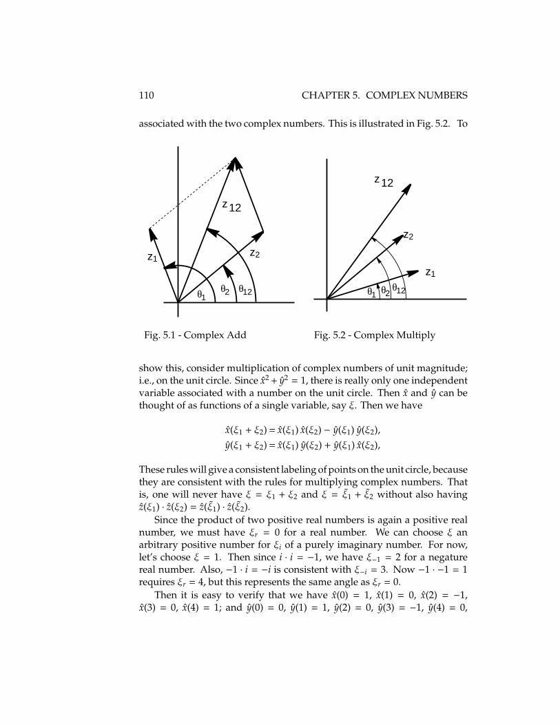
110 CHAPTER 5. COMPLEX NUMBERS
associated with the two complex numbers. This is illustrated in Fig. 5.2. To
z2
z1
z12
θ2θ1θ12
z2z1
z12
θ2θ1θ12
Fig. 5.1 - Complex Add Fig. 5.2 - Complex Multiply
show this, consider multiplication of complex numbers of unit magnitude;i.e., on the unit circle. Since x2 + y2 = 1, there is really only one independentvariable associated with a number on the unit circle. Then x and y can bethought of as functions of a single variable, say ξ. Then we have
x(ξ1 + ξ2) = x(ξ1) x(ξ2) − y(ξ1) y(ξ2),y(ξ1 + ξ2) = x(ξ1) y(ξ2) + y(ξ1) x(ξ2),
These rules will give a consistent labeling of points on the unit circle, becausethey are consistent with the rules for multiplying complex numbers. Thatis, one will never have ξ = ξ1 + ξ2 and ξ = ξ1 + ξ2 without also havingz(ξ1) · z(ξ2) = z(ξ1) · z(ξ2).
Since the product of two positive real numbers is again a positive realnumber, we must have ξr = 0 for a real number. We can choose ξ anarbitrary positive number for ξi of a purely imaginary number. For now,let’s choose ξ = 1. Then since i · i = −1, we have ξ−1 = 2 for a negaturereal number. Also, −1 · i = −i is consistent with ξ−i = 3. Now −1 · −1 = 1requires ξr = 4, but this represents the same angle as ξr = 0.
Then it is easy to verify that we have x(0) = 1, x(1) = 0, x(2) = −1,x(3) = 0, x(4) = 1; and y(0) = 0, y(1) = 1, y(2) = 0, y(3) = −1, y(4) = 0,

5.4. GEOMETRY OF COMPLEX NUMBERS 111
defining positive and negative real numbers, and positive and negativeimaginary numbers.
It is clear that we only have to define x and y in the first quadrant, since,for example
x(ξ + 1) = x(ξ) x(1) − y(ξ) y(1) = −y(ξ).
Then
x(ξ + 1) = −y(ξ), y(ξ + 1) = +x(ξ);x(ξ + 2) = −x(ξ), y(ξ + 2) = −y(ξ);x(ξ + 3) = +y(ξ), y(ξ + 3) = −x(ξ).
Other values for different ξ in the first quadrant can be built up by lettingξ1 = ξ2 = ξ, giving
x(2 ξ) = x2(ξ) − y2(ξ),y(2 ξ) = 2 x(ξ) y(ξ).
or
x(ξ) = x2(ξ2
)− y2
(ξ2
),
y(ξ) = 2 x(ξ2
)y(ξ2
),
leading to
x(ξ2
)= ±
√1 + x(ξ)
2,
while we still have
y(ξ2
)= ±
√1 − x2
(ξ2
).
The sign to use with the square root is determined by which quadrant ofthe circle we are in, since we know what ξ corresponds to the x and y axes.Using these formulas repeatedly, one can calculate x(∆ξ) and y(∆ξ) for assmall ∆ξ as needed, and then calculate x(ξ) from repeatedly applying theexpressions for x(ξ1 + ξ2). For example, we know x(0) = 1 and x(1) = 0.One application gives x(1/2), the next x(1/4), and so on. For example, if wewant x(7/8), we note
x(78
)= x
(12
)x(38
)− y
(12
)y(38
),
y(78
)= x
(12
)y(38
)+ y
(12
)x(38
).
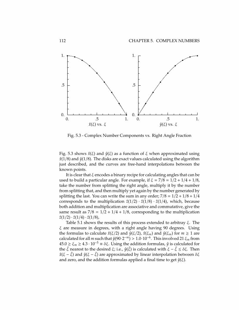
112 CHAPTER 5. COMPLEX NUMBERS
1.
.5
0.0. .5 1.
x(ξ) vs. ξ
r rr
rr
r
r
r
r
1.
.5
0.0. .5 1.
y(ξ) vs. ξ
r
r
r
r
rr
rr r
Fig. 5.3 - Complex Number Components vs. Right Angle Fraction
Fig. 5.3 shows x(ξ) and y(ξ) as a function of ξ when approximated usingx(1/8) and y(1/8). The disks are exact values calculated using the algorithmjust described, and the curves are free-hand interpolations between theknown points.
It is clear that ξ encodes a binary recipe for calculating angles that can beused to build a particular angle. For example, if ξ = 7/8 = 1/2 + 1/4 + 1/8,take the number from splitting the right angle, multiply it by the numberfrom splitting that, and then multiply yet again by the number generated bysplitting the last. You can write the sum in any order; 7/8 = 1/2 + 1/8 + 1/4corresponds to the multiplication z(1/2) · z(1/8) · z(1/4), which, becauseboth addition and multiplication are associative and commutative, give thesame result as 7/8 = 1/2 + 1/4 + 1/8, corresponding to the multiplicationz(1/2) · z(1/4) · z(1/8),
Table 5.1 shows the results of this process extended to arbitray ξ. Theξ are measure in degrees, with a right angle having 90 degrees. Usingthe formulas to calculate x(ξ/2) and y(ξ/2), x(ξm) and y(ξm) for m ≥ 1 arecalculated for all m such that y(90·2−m) > 1.0·10−6. This involved 21 ξm from45.0 ≥ ξm ≥ 4.3 · 10−5 ≡ δξ. Using the addition formulas, y is calculated forthe ξ nearest to the desired ξ; i.e., y(ξ) is calculated with ξ − ξ ≤ δξ. Thenx(ξ − ξ) and y(ξ − ξ) are approximated by linear interpolation between δξand zero, and the addition formulas applied a final time to get y(ξ).

5.4. GEOMETRY OF COMPLEX NUMBERS 113
degs 0 1 2 3 4 5 6 7 8 90 0.000 .0175 .0349 .0523 .0698 .0872 .1045 .1219 .1392 .1564
10 .1736 .1908 .2079 .2250 .2419 .2588 .2756 .2924 .3090 .325620 .3420 .3584 .3746 .3907 .4067 .4226 .4384 .4540 .4695 .484830 .5000 .5150 .5299 .5446 .5592 .5736 .5878 .6018 .6157 .629340 .6428 .6561 .6691 .6820 .6947 .7071 .7193 .7314 .7431 .754750 .7660 .7771 .7880 .7986 .8090 .8192 .8290 .8387 .8480 .857260 .8660 .8746 .8829 .8910 .8988 .9063 .9135 .9205 .9272 .933670 .9397 .9455 .9511 .9563 .9613 .9659 .9703 .9744 .9781 .981680 .9848 .9877 .9903 .9925 .9945 .9962 .9976 .9986 .9994 .9998
Table 5.1: y(ξ) vs. ξ in degrees
By checking with other calculations, it is found that this method gener-ates y(ξ) at the values in the table to an accuracy of approximately 1 in 1010.Before the invention of the inexpensive calculators, tables such as Table 5.1(extended to many more significant figures) were a common method ofworking with these functions in practical calculations.
We would like to supply more of the details of this process. First, wewould like to show that small changes in ξ result in small changes in x(ξ)and y(ξ). And as suggested by Fig. 5.3, we would like to know for sure thatx(ξ)) and y(ξ) are monotonic for 0 ≤ ξ ≤ 1. Let δξ be some small angle usedto build up an arbitrary angle ξ. Then
x(ξ + δξ) = x(ξ) x(δξ) − y(ξ) y(δξ),y(ξ + δξ) = x(ξ) y(δξ) + y(ξ) x(δξ)
and(x(δξ))2 + (y(δξ))2 = 1.
Let
δx(ξ, δξ) = x(ξ + δξ) − x(ξ),δy(ξ, δξ) = y(ξ + δξ) − y(ξ).
We have
δx(ξ, δξ) = x(ξ) (x(δξ) − 1) − y(ξ) y(δξ)
= x(ξ)(x(δξ))2 − 1
x(δξ) + 1− y(ξ) y(δξ)
114 CHAPTER 5. COMPLEX NUMBERS
=−x(ξ)(y(δξ))2
x(δξ) + 1− y(ξ) y(δξ)
=−y(δξ){
x(ξ) y(δξ)x(δξ) + 1
+ y(ξ)}
=−y(δξ){
x(ξ) y(δξ) + y(ξ) x(δξ) + y(ξ)x(δξ) + 1
}
=−y(δξ){
y(ξ + δξ) + y(ξ)x(δξ)) + 1
}.
and
δy(ξ, δξ) = x(ξ) y(δξ) + y(ξ) (x(δξ) − 1)
= x(ξ) y(δξ) + y(ξ)(x(δξ))2 − 1
x(δξ) + 1
= x(ξ) y(δξ) − y(ξ)(y(δξ))2
x(δξ) + 1
= y(δξ){
x(ξ) − y(ξ) y(δξ)x(δξ) + 1
}
= y(δξ){
x(ξ) x(δξ) + x(ξ) − y(ξ) y(δξ)x(δξ) + 1
}
= y(δξ){
x(ξ + δξ) + x(ξ)x(δξ)) + 1
}.
Note also that(x(ξ2
))2=
1 + x(ξ)2
,
1 −(x(ξ2
))2=
1 − x(ξ)2
,
(y(ξ2
))2=
12
1 − (x(ξ))2
1 + x(ξ)
y(ξ2
)=
y(ξ)√2 (1 + x(ξ))
,
or
y(ξ2
)≤ y(ξ)√
2.
Thus y(δξ) can be made as small as desired if we start with ξ = 1.

5.5. CALCULATING PI 115
These calculations show that x(ξ) is monotonically decreasing, and y(ξ)is monotonically increasing, for 0 ≤ ξ ≤ 1. Since δx(ξ, δξ) and δy(ξ, δξ) canbe made as small as desired, they also show that x(ξ + δξ) approaches x(ξ),and y(ξ + δξ) approaches y(ξ), as δξ goes to zero.
We have calculated x(ξ) and y(ξ) by starting with ξ = 1 and repeatedlydividing ξ by two, obtaining x(δξ) and y(δξ) for arbitrarily small δξ. Thenusing the addition formulas, one gets their values at angles that are multi-ples of δξ. Next, one can define x(ξ) and y(ξ) for arbitrary ξ, even thoughwe have explicit expressions for x(ξ) and y(ξ) only at particular points.
To do this, let δξm = 2−m, with m ≥ 0. For fixed ξ, choose nm such thatnm δξm ≤ ξ < (nm + 1) δξm. Define ξ−m = nm δξm and ξ+
m = ξ−m + δξm. Thenfor 0 ≤ ξ ≤ 1, ξ−m is a monotonically increasing sequence with least upperbound ξ−, and ξ+
m is a monotonically decreasing sequence with greatestlower bound ξ+. Since ξ+ − ξ− ≤ ξ+
m − ξ−m = 2−m, which can be made assmall as desired, ξ = ξ− = ξ+.
Since x(ξ) is monotonically decreasing in ξ and ξ+m is monotonically
decreasing in m, x(ξ+m) is monotonically increasing in m. It is also bounded
above by one, so x(ξ+m) converges to a definite number, x(ξ+). Similarly,
x(ξ−m) converges to x(ξ−). But the difference between ξ+ and ξ− approacheszero, and we have shown that this implies that the difference in x(ξ+) andx(ξ−) also approaches zero. This allows one to define x(ξ) ≡ x(ξ+) = x(ξ−).Similar considerations allow us to find y(ξ) for arbitrary ξ.
5.5 Calculating Pi
We have seen that we can consider√
(∆x)2 + (∆y)2 as the distance betweentwo points in the complex plane whose real components differ by ∆x andwhose imaginary components differ by ∆y. Earlier discussions can beseen as a method for dividing an arc of radius 1 describing a right angleinto n = 2m segments corresponding to equal increments δξ by repeatedlyapplying the rule
xm+1 =
√1 + xm
2
and using(xm)2 + (ym)2 = 1
to find the corresponding imaginary component of a small distance smextending from the point Z0,N = 1 to the point Z1,n = xm + ym i. Then one

116 CHAPTER 5. COMPLEX NUMBERS
generates the remaining points on the arc from
Xi+1,n = Xi,n xm − Yi,n ym,
Yi+1,n = Xi,n ym + Yi,n xm.
for i = 1 to n.The circumference of a unit circle is 2π. We would expect to be able to
estimate π by calculating
π2≈
n∑
i=1
√(Xi,n − Xi−1,n)2 + (Yi,n − Yi−1,n)2
for large enough n.But all the terms in this sum are equal, as seen by realizing x = 1, y = 0
at ξ = 0, and writing δy = y(δξ) and δx = x(δξ) − 1. Let
∆x(ξ +
δξ2
)= x(ξ + δξ) − x(ξ),
∆y(ξ +
δξ2
)= y(ξ + δξ) − y(ξ).
Then one writes
∆x(ξ +
δξ2
)= x(ξ) δx − y(ξ) δy,
∆y(ξ +
δξ2
)= x(ξ) δy + y(ξ) δx.
and finds after some algebra
(∆x
(ξ +
δξ2
))2+
(∆y
(ξ +
δξ2
))2
= (x(ξ))2 + (y(ξ))2) · ((δx)2 + (δy)2)= ((δx)2 + (δy)2).
Note that the right hand side is independent of ξ, so that
(∆s)2 =(∆x
(ξ +
δξ2
))2+
(∆y
(ξ +
δξ2
))2= (∆s(δξ))2
depends only on δξ, and is independent of ξ. This means that the intervaldefined by δξ is proportional to a constant distance along the circumferenceof the unit circle independent of its position on the circle. That means we
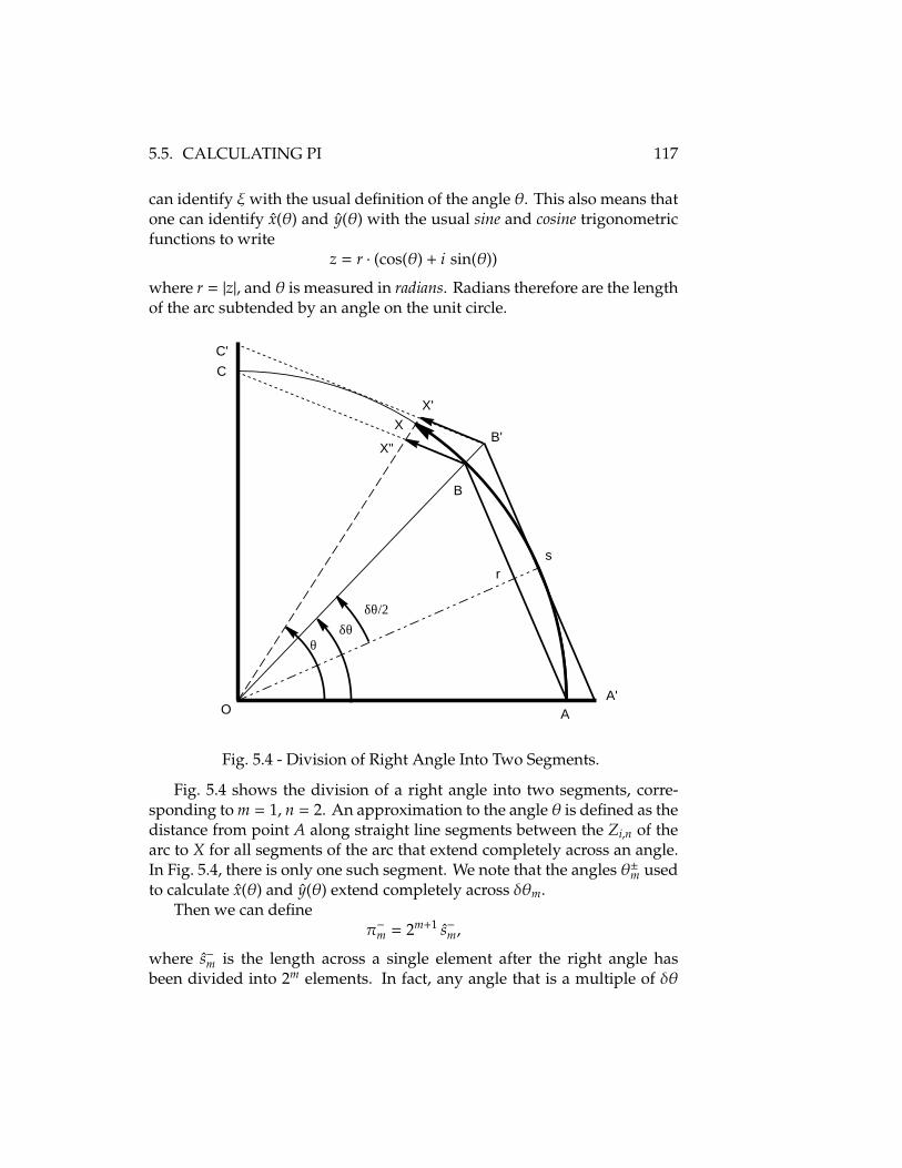
5.5. CALCULATING PI 117
can identify ξwith the usual definition of the angle θ. This also means thatone can identify x(θ) and y(θ) with the usual sine and cosine trigonometricfunctions to write
z = r · (cos(θ) + i sin(θ))
where r = |z|, and θ is measured in radians. Radians therefore are the lengthof the arc subtended by an angle on the unit circle.
O A
B
CC'
B'
A'
XX'
X"
θδθ
δθ/2
rs
Fig. 5.4 - Division of Right Angle Into Two Segments.
Fig. 5.4 shows the division of a right angle into two segments, corre-sponding to m = 1, n = 2. An approximation to the angle θ is defined as thedistance from point A along straight line segments between the Zi,n of thearc to X for all segments of the arc that extend completely across an angle.In Fig. 5.4, there is only one such segment. We note that the angles θ±m usedto calculate x(θ) and y(θ) extend completely across δθm.
Then we can defineπ−m = 2m+1 s−m,
where s−m is the length across a single element after the right angle hasbeen divided into 2m elements. In fact, any angle that is a multiple of δθ

118 CHAPTER 5. COMPLEX NUMBERS
is proportional to the sum of the lengths of all the segments that extendacross segments defined by the δθ. Since all those segments are equal, anyangle can be thought of as the length of a single segment times the numberof segments. As we will now show for a right angle, in the limit that δθapproaches zero, we get a well-defined number—the total length along thearc.
In Fig. 5.4, s−1 is the distance AB. δθ = δθm = δθ1 corresponding to s−1 isthe angle AOB. The line Ors bisects δθ, so that OrB is a right angle. Since OBhas unit length, rB has length y(δθ/2). In general, the mth approximation ofπ will be
π−m = 4 n y(δθm/2) = 2m+2 ym+1.
Then
π−m+1 − π−m = 2m+2 (2 ym+2 − ym+1)
= 2m+2(2
√1 − (xm+2)2 −
√1 − (xm+1)2
)
= 2m+2
2
√1 − 1 + xm+1
2−
√1 − (xm+1)2
= 2m+2(√
2 (1 − xm+1) −√
(1 − xm+1) (1 + xm+1))
= 2m+2√
1 − xm+1
(√2 −
√1 + xm+1
)
= 2m+2 (1 − xm+1)32
√2 +√
1 + xm+1
= 2m+2 (1 − (xm+1)2)32
(1 + xm+1)32 (√
2 +√
1 + xm+1)
= 2m+2 (ym+1)3
(1 + xm+1)32 (√
2 +√
1 + xm+1)
=π−m(ym+1)2
(1 + xm+1)32 (√
2 +√
1 + xm+1)> 0.
So the set of π−m form a monotonically increasing sequence. We expressπ−m+1 − π−m as π−m times a number to show that the difference is a smallfraction of π−m. In this case, we know that xm approaches 1 as m increases,and we know from the fact that we are splitting a small angle on the real axisthat ym is being cut roughly in half each iteration. So we expect π−m+1 − π−mis being cut roughly a factor of 4 each iteration.

5.5. CALCULATING PI 119
If we show that the sequence is bounded above, we will have provedthat π−m converges to a real number π. An upper limit to π can be obtainedby defining s+
1 = A′B′ in Fig. 5.4, and generalizing for s+m. In Fig. 5.4, we see
that the length of Os is 1. Since Os = OB′ · x(δθm/2), the length of OB′ is1/xm+1. Then since B′s = OB′ · y(δθm/2), we have
s+m = 2
ym+1
xm+1
and
π+m − π−m = 2m+2
(ym+1
xm+1− ym+1
)
= 2m+2 ym+1
xm+1(1 − xm+1)
=π+m
(ym+1)2
1 + xm+1
π+m − π−m > 0.
So we have an upper limit on π+m as the minimum value of all the π+
m.However, we can also show that theπ+
m form a monotonically decreasingsequence by considering
π+m+1 − π+
m = 2m+2(2
ym+2
xm+2− ym+1
xm+1
)
= 2m+2
2
√(ym+2)2
(xm+2)2 −ym+1
xm+1
= 2m+2
2
√1 − xm+1
1 + xm+1− ym+1
xm+1
= 2m+2
2
√(1 − xm+1
1 + xm+1
) (1 + xm+1
1 + xm+1
)− ym+1
xm+1
= 2m+2(2
ym+1
1 + xm+1− ym+1
xm+1
)
=−2m+2 ym+1 (1 − xm+1)xm+1 (1 + xm+1)
=−π+m
(ym+1
1 + xm+1
)2
< 0.
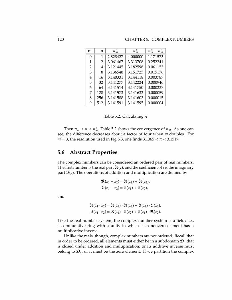
120 CHAPTER 5. COMPLEX NUMBERS
m n π−m π+m π+
m − π−m0 1 2.828427 4.000000 1.1715731 2 3.061467 3.313708 0.2522412 4 3.121445 3.182598 0.0611533 8 3.136548 3.151725 0.0151764 16 3.140331 3.144118 0.0037875 32 3.141277 3.142224 0.0009466 64 3.141514 3.141750 0.0002377 128 3.141573 3.141632 0.0000598 256 3.141588 3.141603 0.0000159 512 3.141591 3.141595 0.000004
Table 5.2: Calculating π
Then π−m < π < π+m. Table 5.2 shows the convergence of πm. As one can
see, the difference decreases about a factor of four when m doubles. Form = 3, the resolution used in Fig 5.3, one finds 3.1365 < π < 3.1517.
5.6 Abstract Properties
The complex numbers can be considered an ordered pair of real numbers.The first number is the real part<(z), and the coefficient of i is the imaginarypart =(z). The operations of addition and multiplication are defined by
<(z1 + z2) =<(z1) +<(z2),=(z1 + z2) ==(z1) +=(z2),
and
<(z1 · z2) =<(z1) · <(z2) − =(z1) · =(z2),=(z1 · z2) =<(z1) · =(z2) +=(z1) · <(z2).
Like the real number system, the complex number system is a field; i.e.,a commutative ring with a unity in which each nonzero element has amultiplicative inverse.
Unlike the reals, though, complex numbers are not ordered. Recall thatin order to be ordered, all elements must either be in a subdomainDp thatis closed under addition and multiplication; or its additive inverse mustbelong to Dp; or it must be the zero element. If we partition the complex

5.7. ROOTS OF COMPLEX NUMBERS 121
plane into two regions, one of which is Dp, consider two numbers that arein Dp. Since multiplication results in adding the angles associated with thetwo numbers, the product will not in general be in Dp. For example, if Dpconsists of the region<(z) > 0, then (1+2 i) ∈ Dp. But (1+2 i)2 = −3+4 i; i.e.,the product of two numbers in Dp is not necessarily in Dp. So the complexnumbers do not separate into positive and negative numbers.
5.7 Roots of Complex Numbers
Consider determining a complex number z satisfying
zn = Z.
with n a positive integer and Z a known complex number. This is a gen-eralization of the problem of determining the square root of a real number.From the fact that the magnitude of the product of complex numbers is theproduct of their magnitudes, we need
|z|n = |Z|,
which involves only real numbers. This can be solved by successive ap-proximations, just as we found
√2 earlier. Then we need only to solve the
equationzn = Z,
where |z| = 1 and |Z| = 1.Recall that multiplying complex numbers corresponds to adding the
associated angles. If we have a number n√1+, with∣∣∣ n√1+
∣∣∣ = 1 and whoseassociated angle is the nth part of a circle around the origin of the complexplane, then
(n√1+
)n= 1. As a matter of fact,
(n√1+
)mfor 0 ≤ m < n also
satisfies((
n√1+)m)n
= 1 (where(
n√1+)0 ≡ 1). This follows from
(( n√1+
)m)n=
( n√1+
)mn=
( n√1+
)nm=
(( n√1+
)n)m= 1m = 1.
We note the angle associated with(
n√1+)m
is m times the angle associated
with n√1+, so the(
n√1+)m
are distinct for 0 ≤ m < n. If one chooses m ≥ n,
one just reproduces(
n√1+)m−n
.

122 CHAPTER 5. COMPLEX NUMBERS
To solve zn = Z, define a n√Z with∣∣∣ n√Z
∣∣∣n = |Z| and an associated anglethe nth part of the angle associated with Z. Then there are n solutions to
zn = Z,
namely,zm =
n√Z
( n√1+
)m, 0 ≤ m < n.
For example, let’s look at z2 = i directly. With z = x + y i, we have
(x2 − y2) + 2 x y i = i,
or
y =±x,±2 x2 = 1.
But only the positive sign is possible in the second equation since x is real.Then the two roots are given by
z = ± 1√2
(1 + i).
In this case2√
i =1√2
(1 + i),
and multiplying by 2√1+ = −1 gives the other root.
5.8 Quadratic Equations
The complex numbers were invented to solve equations that required anumber whose square is negative. This arises in many solutions of thequadratic equation
a x2 + b x + c = 0,
which, in turn, arises in many practical applications.One can solve this equation by taking advantage of the algebraic prop-
erties of a field:
a x2 + b x =−c,
x2 +ba
x =−ca,
5.9. THE FUNDAMENTAL THEOREM OF ALGEBRA. 123
(x +
b2 a
)2
=−ca
+b2
4 a2 ,
x +b
2 a=±
√b2 − 4 a c
4 a2 ,
x =−b ±
√b2 − 4 a c
2 a.
If 4 a c > b2, there is no solution in the field of real numbers, even though allthe coefficients are real numbers
Now, all the algebraic steps that were used above can be used for equa-tions with complex coefficients. This is true because the complex numbersform a fields, just like the real numbers. That is, there are additive inverses,so one can add the same quantity to each side of an equation. There aremultiplicative inverses, so one can divide each side by any nonzero number.But there are also complex numbers whose square are negative, and hencethe last step is always justified if a , 0.
For example, one finds easily enough that the two solutions of
x2 − 3 x + 2 = 0
are x = 1 and x = 2. Direct application of the above result to
x2 − 3 x i − 2
shows x = i and x = 2 i are solutions of an equation with complex coeffi-cients.
For equations with real coefficients, there is also an interesting change indescription possible. We can say that there are either two real solutions, onereal solution (if 4 a c = b2), or no real solutions. If we work in the complexnumber system, we can say there are always two solutions, which may bedegenerate if 4 a c = b2. Furthermore, we see complex roots are complexconjugates of each other.
5.9 The Fundamental Theorem of Algebra.
We have shown that the roots of an arbitrary quadratic can be calculatedexplicitly. It is easy to believe that a generalization to higher order poly-nomials would quickly get very messy. However, it turns out that it is notdifficult to show that an nth-order polynomial has n roots, which may in
124 CHAPTER 5. COMPLEX NUMBERS
general be complex.1 This means that an nth-order polynomial
pn(z) =
n∑
i=0
an−i zn−1
can be written in the form
pn(z) = an (z − z1) (z − z2) . . . (z − zn),
where some of the zi may be the same; i.e., degenerate. This is known asT F T A. Also, if we are only interested infinding the roots zi, we are free to choose an = 1 by dividing each of theother ai by an , 0, (otherwise the polynomial is of lower order than n).
First we show that an nth-order polynomial can be written in the form
pn(z) = (z − zn) pn−1(z),
where pn−1(z) is of order n − 1, if pn(zn) = 0. This process can be continuedwith pn−1(z) until we have the desired form.
We note that if pn(z) can be written in this form, choosing z = zi for somezi solves the equation pn(z) = 0. But it doesn’t automatically follow logicallythat zn such that pn(zn) = 0 implies that pn(z) can be written as (z−zn) pn−1(z).However, this does follow from the fact that it is possible to write down theexplicit form of pn−1(z), given pn(z) and zn. This follows from the algebraicidentity
zm − zmn = (z − zn) · (zm−1 + zm−2 zn + zm−3 z2
n + . . . + zm−1n )
= (z − zn)m−1∑
i=0
zm−i−1 zin.
This allows one to write zm in terms of zmn plus a term proportional to z− zn
times a factor with z raised to a power less than m. Thus one simply replaceszm by zm − zm
n + zmn in pn(z), where pn(zn) = 0, and rearranges the resulting
series.For example, consider the quadratic equation
p2(z) = z2 + a1 z + a0
= (z2 − z22 + z2
2) + a1 (z − z2 + z2) + a0
= (z − z2) (z + z2) + a1 (z − z2) + z22 + a1 z2 + a0
= (z − z2) (z + z2 + a1) + z22 + a1 z2 + a0
= (z − z2) (z + z2 + a1) + p2(z2).1For example, see Courant and Robbins in the Bibliography.

5.9. THE FUNDAMENTAL THEOREM OF ALGEBRA. 125
150
−100
−50
0
50
100
150
−150 −100 −50 0 50 100−150
6
−8
−6
−4
−2
0
2
4
6
8
10
−14−12−10−8 −6 −4 −2 0 2 4−10
Fig. 5.5 - P(z), z2 for |z| = 10 Fig. 5.6 - P(z) for |z| = 1.8, 2.2
But if p2(z2) = 0, we have
p2(z) = (z − z2) p1(z)
withp1(z) = z + (z2 + a1).
We illustrate a method to find at least one root of a polynomial byconsidering this quadratic equation with
z1 = .6 + .8 i,z2 =−1 +
√3 i
The method is a generalization of a procedure that brackets the solutionbetween an upper and lower limit. The complication here is that the poly-nomial is a function of both the real and imaginary parts of z. This compli-cation is handled by fixing the magnitude of z and considering the behaviorof the polynomial as a function of θ; i.e., we write z = r · (cos(θ) + sin(θ) i),fix r and look at the p(z) as a function of θ.
A key observation is that as θ changes from 0 to 2π, zn returns to itsinitial value when n is an integer. So any polynomial in z will form a closedpath in the complex plane. Furthermore, when r is large enough, we see thatzn dominates, so pn(z) for large enough |z| circles the origin of the complexplane n times.
This is illustrated in Fig. 5.5, which plots this polynomial for |z| = 10. Thedashed line is a corresponding plot of z2, which of course has the segment

126 CHAPTER 5. COMPLEX NUMBERS
for π ≤ θ ≤ 2π overlaying the segment for 0 ≤ θ ≤ π. The differencebetween the dashed line and the solid line represents the contribution ofthe lower-order terms of the polynomial.
In addition, if |z| is small enough, The curves converge on a specificpoint,
a0 = (−1)n z1 z2 . . . zn.
Polynomials in z also vary smoothly as we move from point to point. Thatis, a polynomial at z differs from the same polynomial at z + δz by a termproportional to δz, which can be made as small as desired by moving closerto z. For example
(z + δz)2 = z2 + δz · (2 + δz).
Thus a polynomial has no discontinuous changes in value, as we movealong a path between two points. Therefore the path traced by the poly-nomial in Fig. 5.5 will sweep out the entire interior of that path (withoutleaving uncovered areas in the z plane) as |z| decreases to 0, and the poly-nomial converges on a0.
Next, Fig. 5.6 shows the behavior of the polynomial for |z| = 2.2 and1.8, values which bracket the root z2. If |z| is the magnitude of a root, thecurve must pass through the origin of the complex plane, corresonding to|p(z)| = 0. In addition, the “x” indicates a0 for this equation.
Notice that we can tell when decreasing |z| causes the curve to passthrough the origin. If we drawn a straight line from the origin to the curve,and let the end of the line on the curve follow θ as θ increases while theother end remains at the origin, the line will circle around the origin likethe hands of a clock. If |z| is large enough, as in Fig. 5.5, the line will rotaten time because pn(z) is never zero on the curve.
Notice that this is also true for |z| = 2.2, the dashed curve in Fig. 5.6However, the line only rotates once after we have decreased |z| to 1.8 (al-though it does reverse direction once), because we have passed through theorigin once. The number of times this line rotates about the origin of thecomplex plane is called the winding number of the curve.
For a general function, it might be possible for a curve with 1.8 < |z| < 2.2in Fig. 5.6 to jump discontinuously over the origin as we move between thetwo in the figure, changing the winding number without passing throughthe origin. But the winding number of a smoothly varying function onlychanges when the curve passes through the origin. So we can discoverwhen the curve has passed through a root as |z| changes by monitoring thewinding number. Once we find a curve for which pn(|z|) = 0, one can findthe value of θ that corresponds to the root.

5.10. SUMMARY 127
The winding number for curves of small enough |z| is zero. Thus thewinding number of the curve must decrease as we reduce |z| from a valuethat has a winding number of n. Since the polynomial varies smoothly,that can happen only if the curve does in fact pass through the origin. Thisshows that our polynomial has a root.
Lastly, we would point out that if the coefficients of the polynomial arereal, complex roots appear in complex conjugate pairs. That is if one of theroots zi is complex, then the complex conjugate of zi is also a root. Thisfollows from the fact that the nth power of the complex conjugate is equalthe complex conjugate of the nth power. For example,
((x + i y)2)∗ = (x2 − y2 + i 2 x y)∗ = x2 − y2 − i 2 x y = (x − i y)2.
5.10 Summary
We have extended the field of real numbers to include square roots of neg-ative numbers. The complex numbers have the usual algebraic propertiesof real numbers, except that they are not ordered.
A complex number has a real part and an imaginary part. A complexnumber has associated with it a complex conjugate and a real numbercalled the magnitude or absolute value. The magnitude of the sum of twocomplex numbers is less than or equal to the sum of the magnitudes of thetwo numbers. The magnitude of the product of two complex numbers isthe product of the magnitude of the two factors. Zero is the only complexnumber that has zero magnitude.
Each complex number can be considered a point in a two-dimensionalplane. An angle in the counterclockwise sense can be associated betweenthe positive real axis and a line from the origin to the point. Multiplicationof two complex numbers gives a product whose associated angle is the sumof the angles of the factors.
We have shown that the algebra of complex numbers is consistent withgeometry in two dimensions. We have shown that the Pythagorean Theo-rem of geometry follows as a consequence of this algebra. As a result, π,the ratio of the circumference of a circle to its diameter, can be calculated.
We have given an explicit formula two solutions of a quadratic equation,although the roots may be degenerate. If the coefficients of the equation arereal and the roots are distinct and complex, they are complex conjugates ofeach other.
We have examined the general nth root of a complex number, and haveshown that n distinct roots exist. There are also n roots (some possibly
128 CHAPTER 5. COMPLEX NUMBERS
degenerate) for an nth-order polynomial, a fact know as the FundamentalTheorem of Algebra. Complex roots of polynomials with real coefficientsoccur in complex-conjugate pairs.

Appendix A
Addendum
In the last chapter, we showed how to raise a complex number to a power,given that the power was a real number. That is, we showed how to calculatezx for z complex if x is real. It turns out to be of considerable practicalimportance, in many fields of applied math, science and engineering, to beable to do the converse; i.e., to raise a real number to a complex power.This means we need to decide what xz means. But first we look at usefulapplications of raising real numbers to real powers.
A.1 Exponential and Logarithmic Tables
Recall that xn, where n is a natural number, means to multiply x by itself ntimes. This means xm+n = xm xn. This property can be generalized. Sincexn = xn+0 = xn x0. we define x0 ≡ 1, Then 1 = x0 = xn−n = xn x−n impliesx−n = 1/xn. Also, since xm·n = (xn)m, it is natural to write for positivex = x1 = (x1/n)n, so that x1/n is the nth root of any positive x. To avoidany complications of complex roots of negative numbers, in this section weassume that we are talking about a real x > 0.
Then for any positive rational number y = m/n, one can define
xy = xm/n = (x1/n)m,
i.e., xm/n is the nth root of x raised to the mth power. This process canbe defined for a real number given as a converging sequence of rationalnumbers, as we did for defining
√2.
Raising a real number to a fractional power can be a useful computa-tional technique. If u = ax and v = ay, then
u · v = ax · ay = ax+y,
129

130 APPENDIX A. ADDENDUM
10.
5.
0.0. .5 1.
10x vs. x
q q qq
q
q
q 1.
.5
0.0. 5. 10.
log10(x) vs. x
q
Fig. A.1 - Exponential and Logarithmic Functions
and there exists a number w such that w = u ·v = ax+y. If we can determine xand y from u and v, and w from x+ y more easily than actually multiplying utimes v, we have a potentially useful calculational tool. The number we arelooking for is the logarithm of a number, written loga(w), and it is defined byw = aloga(w). The number a is called the base of the logarithm. If the numbera is not written, it is assumed that the base is 10, and the logarithms arecalled the common logarithms.
Some logarithms are easy to determine. For example, loga(1) = 0 andloga(a) = 1. Since 10
12 =√
10, we have log√
10 = 12 . So because it is easy
to calcuate the square root of a number, it is easy to calculate logarithmsof 102−m
(m integer) and products of such terms.. Thus, we can show ingeneral what the common exponential and logarithmic functions look likein Fig. A.1. The values at the dots are exact values, calculated from multiples
of 102−3= 101/(23) = 101/8 =
8√10 =
√√√10 = 1.3335 . . ., and the curves are
interpolated free-hand between points.Tables A.1 and A.2 show tables that are constructed using an extension
of this procedure. The difference between the tables and the figures is thatfor the figures, we have plotted values at exactly known points.
For Table A.1, we specify x at particular values, and ask for 10x at thosevalues. This is done by writing
x =
n∑
m=1
xm 2−m,
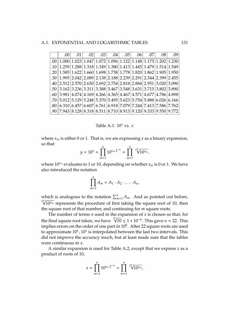
A.1. EXPONENTIAL AND LOGARITHMIC TABLES 131
.00 .01 .02 .03 .04 .05 .06 .07 .08 .09.00 1.000 1.023 1.047 1.072 1.096 1.122 1.148 1.175 1.202 1.230.10 1.259 1.288 1.318 1.349 1.380 1.413 1.445 1.479 1.514 1.549.20 1.585 1.622 1.660 1.698 1.738 1.778 1.820 1.862 1.905 1.950.30 1.995 2.042 2.089 2.138 2.188 2.239 2.291 2.344 2.399 2.455.40 2.512 2.570 2.630 2.692 2.754 2.818 2.884 2.951 3.020 3.090.50 3.162 3.236 3.311 3.388 3.467 3.548 3.631 3.715 3.802 3.890.60 3.981 4.074 4.169 4.266 4.365 4.467 4.571 4.677 4.786 4.898.70 5.012 5.129 5.248 5.370 5.495 5.623 5.754 5.888 6.026 6.166.80 6.310 6.457 6.607 6.761 6.918 7.079 7.244 7.413 7.586 7.762.90 7.943 8.128 8.318 8.511 8.710 8.913 9.120 9.333 9.550 9.772
Table A.1: 10x vs. x
where xm is either 0 or 1. That is, we are expressing x as a binary expansion,so that
y = 10x =
n∏
m=1
10xm 2−m=
n∏
m=1
2m√10xm ,
where 10xm evaluates to 1 or 10, depending on whether xm is 0 or 1. We havealso introduced the notation
n∏
m=1
Am = A1 · A2 · . . . · An,
which is analogous to the notation∑n
m=1 Am. And as pointed out before,2m√
10xm represents the procedure of first taking the square root of 10, thenthe square root of that number, and continuing for m square roots.
The number of terms n used in the expansion of x is chosen so that, forthe final square root taken, we have 2n√
10 ≤ 1 + 10−6. This gave n = 22. Thisimplies errors on the order of one part in 106. After 22 square roots are usedto approximate 10x, 10x is interpolated between the last two intervals. Thisdid not improve the accuracy much, but at least made sure that the tableswere continuous in x.
A similar expansion is used for Table A.2, except that we express x as aproduct of roots of 10,
x =
n∏
m=1
10xm 2−m=
n∏
m=1
2m√10xm ,

132 APPENDIX A. ADDENDUM
.0 .1 .2 .3 .4 .5 .6 .7 .8 .91.0 .0000 .0414 .0792 .1139 .1461 .1761 .2041 .2304 .2553 .27882.0 .3010 .3222 .3424 .3617 .3802 .3979 .4150 .4314 .4472 .46243.0 .4771 .4914 .5052 .5185 .5315 .5441 .5563 .5682 .5798 .59114.0 .6021 .6128 .6233 .6335 .6435 .6532 .6628 .6721 .6812 .69025.0 .6990 .7076 .7160 .7243 .7324 .7404 .7482 .7559 .7634 .77096.0 .7782 .7853 .7924 .7993 .8062 .8129 .8195 .8261 .8325 .83887.0 .8451 .8513 .8573 .8633 .8692 .8751 .8808 .8865 .8921 .89768.0 .9031 .9085 .9138 .9191 .9243 .9294 .9345 .9395 .9445 .94949.0 .9542 .9590 .9638 .9685 .9731 .9777 .9823 .9868 .9912 .9956
Table A.2: log(x) vs. x
rather than a sum of negative powers of 2. Then
x = 10y = 10log(x)
gives
y = log(x) =
n∑
m=1
xm 2−m.
Here’s a simple example of how the tables might be used to reducemultiplication to addition. Look at 15 · 62 = 930. We have
log(15) = log(10 · 1.5)= log(10) + log(1.5)= 1 + .1761= 1.1761
log(62) = 1.7924,log(15 · 62) = log(15) + log(62)
= 2.9685,102.9685 = 102 · 10.9685
= 100 · 9.30= 930.
Note that even in multiplication of 2-digit numbers, the product mayhave more digits than are explicitly given in the tables; e.g., 16 · 62 = 992.
A.1. EXPONENTIAL AND LOGARITHMIC TABLES 133
But the tables give log(16 · 62) = 2.9965. From Table A.1 all we know forsure is that the product is between 990 and 1000.
We can try interpolation, noting that log 990 = 2.9956 and log 1000 = 3.Suppose y = 10x and y + ∆y = 10x+∆x, where x, y, x + ∆x and y + ∆y areknown. In this case, we have y = 9.9 and ∆y = .1, with x and x + ∆x thecorresponding logarithms. We know x + δx, and want to interpolate to gety + δy = 10x+δx.
It is intuitively clear that if we linearize between known values, weshould end up with a linear relationship between δy and δx. In fact, wewould guess that
δy∆y
=δx∆x.
To show that this is true, begin with
10x+δx = (1 − α) 10x + α 10x+∆x,
10δx/x = (1 − α) + α 10∆x/x,
1 + βδxx≈ 1 + αβ
(∆xx
),
where β is a constant. Then
α ≈ δx∆x,
and
10x+δx ≈ 10x + α(10x+∆x − 10x
),
y + δy≈ y + α∆y,δy≈ α∆y,
as expected.Since
2.9965 − log(990)log(1000) − log(990)
=2.9965 − 2.9956
3 − 2.9956=
944≈ .2,
an interpolation would give log(16·62) ≈ log(992). Thus we might hope thatinterpolation can be used to give (n + 1)-digit accuracy from n-digit tables,if the logarithms of the n-digit numbers are given with sufficient accuracy.One notes that it doesn’t take much paper to display 2-digit tables. Threedigit tables would only be a few pages long, and for more important workit would be reasonable to use tables for 4-digit numbers. It is easy to verifythat multiplying 4-digit numbers is quite a bit more tedious than adding

134 APPENDIX A. ADDENDUM
them, so one can easily understand why tables such as these were usedbefore calculators became common.
Recall that xn, where n is a natural number, means to multiply x by itselfn times. This means xm+n = xm xn. This property can be generalized. Sincexn = xn+0 = xn x0, we define x0 ≡ 1. Then 1 = x0 = xn−n = xn x−n impliesx−n = 1/xn. Also, since xm·n = (xn)m, it is natural to write for positivex = x1 = (x1/n)n, so that x1/n is the nth root of any positive x.
A.2 Natural Logarithms
It is useful to show how the use of common logarithms, Table A.1, allowsone to determine logarithms to any base. Note that we can write either
x = aloga(x),
orx = 10log(x).
But notice thatxy =
(aloga(x)
)y= ay loga(x),
so thatlog (xy) = y log(x).
Then we havelog(x) = log
(aloga(x)
)= loga(x) log(a).
This gives a method of converting the common logarithms to logarithms ofany other base; i.e.,
loga(x) =log(x)log(a)
.
It turns out that there is a particular base for logarithms that has a veryuseful property. It is clear from Fig. A.1 that near x ≈ 0, we have a linearrelationship between 10x and x, so we can write
10x ≈ 1 + β x,
where β a constant, for x� 1 (x much less than 1). Converting to a differentbase would give
ax = 10x log(a) ≈ 1 + β log(a) x.
Choose a = e such that β log(e) = 1. This choice of a defines e such that
ex ≈ 1 + x,
A.2. NATURAL LOGARITHMS 135
for small enough x.From Table A.1, we see that 10x increases .023 as x goes from 0 to .01.
Then
1log(e)
≈ 2.3,
log(e)≈ .434,
so thate ≈ 10.434 ≈ 2.7.
To get a more accurate determination of e, it is useful to get an estimatein the error in determining β = 1/ log e. We can do this by calculating 10δx
for a small enough δx that 10δx is essentially linear in δx. We assume that10δx is essentially linear when 10δx < 1 + ε, where ε is a number of the sameorder of magnitude as δx.
It is convenient to choose δx = 2−m, so that
10δx = 102−m=
2m√10,
since we can calculate 2m√10 for any m. Then since
10x =1
10−x ,
we can determine two possible values of β from
1 + βam 2−m ≈ 2m√
10 ≈ 11 − βb
m 2−m
Then we have
βam =
102−m − 12−m ,
βbm =
102−m − 12−m 102−m .
An estimate in the uncertainty in β is given by
∆βm = βam − βb
m =
(102−m − 1
)2
2−m 102−m =
(βa
m)2
102−m 2−m ≈ (βa
m)2 2−m,
where we have used 102−m ≈ 1.

136 APPENDIX A. ADDENDUM
We can get an estimate of the error in e implied by βam and βb
m from
∆em = 101βa
m − 101βb
m
= 101βa
m
1 − 10
(1βb
m− 1βa
m
)
= 101βa
m
(1 − 10
∆βmβa
m βbm
)
≈−eam
∆βm
βam
≈−eam β
am 2−m,
where we have used the linear approximation of the exponential involvingthe small quantity ∆βm, and replaced βb
m by βam when convenient.
For example, if we choose ε = 10−6, one finds m = 22,
eam ≈ 2.718281
ebm ≈ 2.718283
∆em ≈−1.5 × 10⁻⁶,
where eam = 101/βa
m , and similarly for ebm. One can verify that e is very nearly
the average of the two, which is consistent with the estimate of ∆em.The property
ex ≈ 1 + x,
for x ≈ 0 turns out to be so useful that one defines natural logarithms by thespecial notation
ln(x) ≡ loge(x).
In fact, one often describes e as the base of the natural logarithms. So wenow have two special cases of loga(x): log(x) ≡ log10(x), and ln(x) ≡ loge(x).
Growth of a number that, at any instant, is proportional to the numberitself is an example of why e is a useful number. For example, suppose apopulation is increasing 5% a year. Clearly, the rate of increase is propor-tional to the population y at the beginning of the year. If the population y′
at the end of the year isy′ = (1 + α′) y,
and if α′ � 1, we have y′ ≈ y eα′. As a matter of fact, we can write y′ = y eα,
where α ≈ α′ for α� 1. We just write
y′ = eα y,

A.3. DEFINING PROPERTY OF EXPONENTIALS 137
eα y = (1 + α′) y,α= ln(1 + α′).
Furthermore, if we ask for an estimate of the population y at the middleof the year,1 we would guess
y = (1 + .5α′) y.
This gives y ≈ e.5α′
y. In general, if we measure the passage of time t inyears, we would expect
y(t) = eα t y0,
where y0 = y(t = 0). We could do the entire calculation raising 10 to somepower, but numerical factors of ln(10) or log(e) would multiply the rates.So using e just simplifies the calculations.
A.3 Defining Property of Exponentials
Returning now to the probem raised at the beginning of this chapter, wewould like to determine how to raise a real number to a complex power.Of course, the problem is that if the exponent n in xn is complex, we don’thave the idea of multiplying x a complex number of times. It turns out thatthe generalization of this operation is to take one of the properties of theoperation with real numbers, and make it the defining property of a newfunction. To see how this is done, let us define a function
fa(x) = ax,
where a is arbitrary and x is a real number. Then fa(x) satisfies
fa(x + y) = fa(x) · fa(y).
This property, which is obvious for real x and y, can be generalized to thecase where x and y are complex. The new function with this property is theexponential function exp(x), and the defining property is written
exp(x + y) = exp(x) · exp(y),
where clearly we want to define exp(0) = 1 so that exp(x+0) = exp(x)·exp(0).
1Making the highly idealistic assumption that births occur uniformly throughout theyear.
138 APPENDIX A. ADDENDUM
We note that the function exp(x) has the property of raising a number toa power. For example, we define exp(1) by
exp(1) ≡ e.
Nowe2 = exp(1) · exp(1) = exp (1 + 1) = exp(2),
so exp(2) raises the number e to the second power. Furthermore, exp(1/2)is the square root of e, since
exp(12
)· exp
(12
)= exp
(12
+12
)= exp(1) = e.
So in general for positive integers x and y,
exp(
xy
)= exp
(1y
+1y
+ · · ·)
︸ ︷︷ ︸x times
= exp(
1y
)· exp
(1y
)· · ·
︸ ︷︷ ︸x times
has the expected interpretation of the yth root of e raised to the xth power.The number exp(x) turns out to be the limit of a sequence of numbers,
similar to the manner that√
2 is the limit of a sequence of rational numbers.We will discover that sequence for exp(x) by writing it as a product of termsthat differ slightly from 1 = exp(0). We write
exp(x) = exp(n · x
n
)=
(exp
(xn
))n.
Note that xn can be made as small as desired. Furthermore, on a fine enough
scale, any “reasonable” function looks like a straight line.We can elaborate on this a bit. Fig. A.2 gives a plot of
f (x) = sin(
1√x2 + δ2
)
with δ = .005. We know from the previous chapter that, in general, sin(θ) =x(θ) is a well-defined function if θ is well-defined. However, in this caseθ = 1/
√x2 + δ2. If δ = 0, f (x) would not be defined at all at x = 0. With δ
small, the function oscillates increasingly rapidly near x = 0. It might notbe clear that this function looks like a straight line on a small scale. ButFig. A.3 shows the f (x) when the scale of x is expanded a factor of 100. On
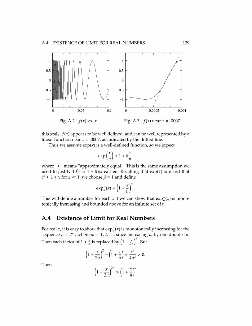
A.4. EXISTENCE OF LIMIT FOR REAL NUMBERS 139
0.1
−0.5
0
0.5
1
0 0.05
−1
0.001
−0.5
0
0.5
1
0 0.0005
−1
Fig. A.2 - f (x) vs. x Fig. A.3 - f (x) near x = .0007
this scale, f (x) appears to be well defined, and can be well represented by alinear function near x = .0007, as indicated by the dotted line.
Thus we assume exp(x) is a well-defined function, so we expect
exp(xn
)≈ 1 + β
xn,
where “≈” means “approximately equal.” This is the same assumption weused to justify 10δx ≈ 1 + β δx earlier. Recalling that exp(1) ≡ e and thatex ≈ 1 + x for x� 1, we choose β = 1 and define
exp−n (x) =(1 +
xn
)n.
This will define a number for each x if we can show that exp−n (x) is mono-tonically increasing and bounded above for an infinite set of n.
A.4 Existence of Limit for Real Numbers
For real x, it is easy to show that exp−n (x) is monotonically increasing for thesequence n = 2m, where m = 1, 2, . . ., since increasing m by one doubles n.
Then each factor of 1 + xn is replaced by
(1 + x
2n
)2. But
(1 +
x2n
)2−
(1 +
xn
)=
x2
4n2 > 0.
Then (1 +
x2n
)2n>
(1 +
xn
)n

140 APPENDIX A. ADDENDUM
andexp−2n(x) > exp−n (x).
We use a trick to show that exp−n (x) has an upper limit. Recall that wewant
1 = exp(0)
exp(x) · 1exp(x)
= exp(x − x)
exp(x) · 1exp(x)
= exp(x) · exp(−x)
1exp(x)
= exp(−x),
orexp(x) =
1exp(−x)
.
This suggests that if exp−n (x) is monotonically increasing, then
exp+n (x) ≡ 1
exp−n (−x)=
1(1 − x
n
)n
would be expected to be monotonically decreasing. Indeed, we have
1(1 − x
2n
)2 −1
1 − xn
=− x2
4n2(1 − x
2n
)2 (1 − x
n
) ,
so in fact exp+n (x) is monotonically decreasing if n ≥ n0 > x, where we have
already assumed x > 0. In the rest of the section, we will assume that n ≥ n0,so that exp+
n (x) > 0; i.e., it is bounded below. Then we have the existence of
exp+(x) = limn→∞ exp+
n (x).
Since1
1 − xn
−(1 +
xn
)=
x2
n2 ·1
1 − xn
,
we have1
1 − xn
> 1 +xn,
A.4. EXISTENCE OF LIMIT FOR REAL NUMBERS 141
andexp+
n (x) > exp−n (x).
This shows that exp−n (x) has an upper limit.2 It is also the reason for thesuperscripts “+” and “−,” for exp+
n (x) approaches its limit from above,and exp−n (x) approaches its limit from below. Thus we are also justified indefining
exp−(x) = limn→∞ exp−n (x),
We can show that exp−n (x) and exp+n (x) have the same limit (again, for
real x) by using the identity
an − bn = (a − b) · (an−1 + an−2 b + an−3 b2 + . . . + bn−1)
= (a − b)n−1∑
m=0
an−1−m bm.
Then
exp+n (x) − exp−n (x) =
1
1 − xn
−(1 +
xn
)
n−1∑
m=0
(1 +
xn
)n−m−1 (1 − x
n
)−m.
The first term on the right is
x2
n21
1 − xn
.
Now (1 +
xn
)n−m−1 (1 − x
n
)−m<
(1 − x
n
)−(n−1)
and (1 +
xn
)n−m−1 (1 − x
n
)−m<
(1 − x
n
)exp+
n (x).
There are n terms of this form, giving
exp+n (x) − exp−n (x) <
x2
n1
1 − xn
exp+n (x).
2 Consider also exp−n (x) and exp+m(x) for m , n. If m > n, note that exp+
m(x) > exp−m(x),while exp−m(x) > exp−n (x), which implies exp+
m(x) > exp−n (x). Similarly, if m < n, thenexp+
m(x) > exp+n (x), while exp+
n (x) > exp−n (x), also leads to exp+m(x) > exp−n (x). Therefore since
exp+n0
(x) is an upper bound for all exp+n (x), it is also an upper bound for all exp−n (x).
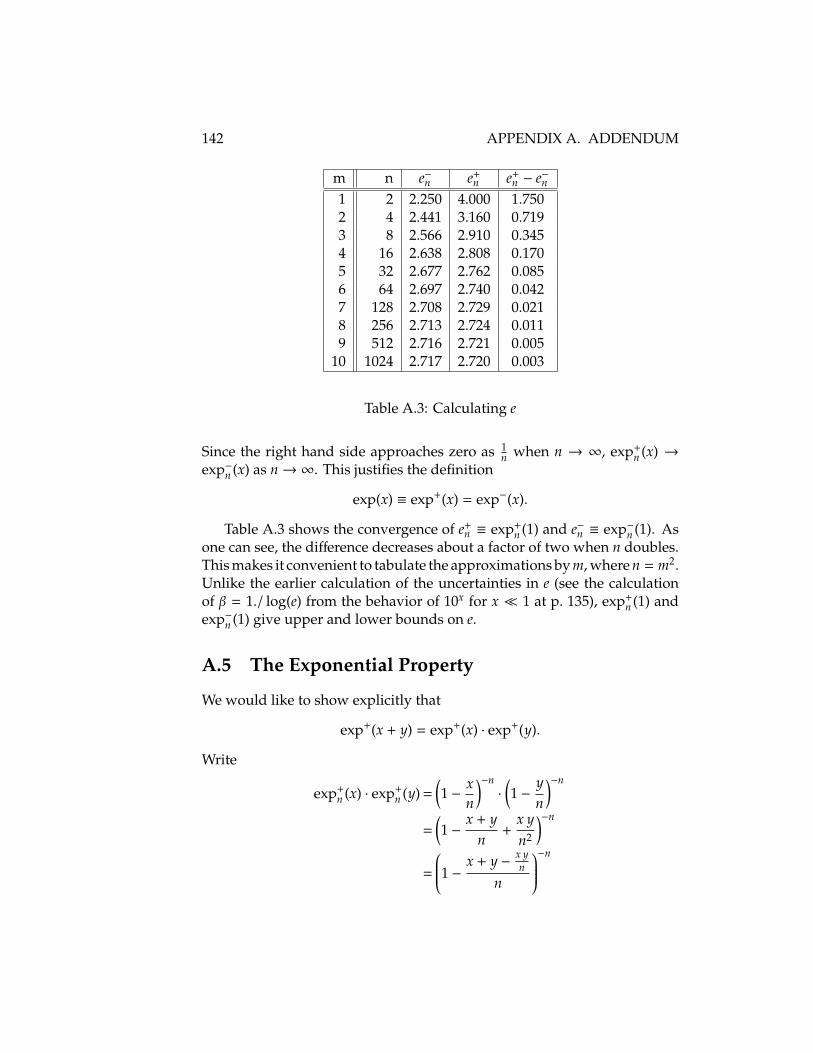
142 APPENDIX A. ADDENDUM
m n e−n e+n e+
n − e−n1 2 2.250 4.000 1.7502 4 2.441 3.160 0.7193 8 2.566 2.910 0.3454 16 2.638 2.808 0.1705 32 2.677 2.762 0.0856 64 2.697 2.740 0.0427 128 2.708 2.729 0.0218 256 2.713 2.724 0.0119 512 2.716 2.721 0.005
10 1024 2.717 2.720 0.003
Table A.3: Calculating e
Since the right hand side approaches zero as 1n when n → ∞, exp+
n (x) →exp−n (x) as n→∞. This justifies the definition
exp(x) ≡ exp+(x) = exp−(x).
Table A.3 shows the convergence of e+n ≡ exp+
n (1) and e−n ≡ exp−n (1). Asone can see, the difference decreases about a factor of two when n doubles.This makes it convenient to tabulate the approximations by m, where n = m2.Unlike the earlier calculation of the uncertainties in e (see the calculationof β = 1./ log(e) from the behavior of 10x for x � 1 at p. 135), exp+
n (1) andexp−n (1) give upper and lower bounds on e.
A.5 The Exponential Property
We would like to show explicitly that
exp+(x + y) = exp+(x) · exp+(y).
Write
exp+n (x) · exp+
n (y) =(1 − x
n
)−n·(1 − y
n
)−n
=(1 − x + y
n+
x yn2
)−n
=
1 − x + y − x yn
n
−n

A.5. THE EXPONENTIAL PROPERTY 143
= exp+n
(x + y − x y
n
)
In the limit that n→∞, we expect that
exp+(x) · exp+(y) = exp+(x + y).
To show this, first note that
exp+n(x + y
) ≥ exp+n
(x + y − x y
n
)≥ exp+
n
(x + y − x y
m
).
for n > m (and x y ≥ 0). Letting n→∞, we have
exp(x + y) ≥ limn→∞ exp+
n
(x + y − x y
n
)≥ exp
(x + y − x y
m
).
Then letting m→∞, we expect
exp(x + y) ≥ limn→∞ exp+
n
(x + y − x y
n
) ?≥ exp(x + y),
To justify the last relationship, we need to show
limδ→0
exp(x + δ) = exp(x),
with δ = −x ym . This property is called continuity, and functions with this
property are continuous. To see why this is necessary, consider a function
f (x) =
1 if x > 00 if x = 0−1 if x < 0
For x = 0, it is clear that limδ→0 f (x + δ) , f (x). One says that f (x) iscontinuous except at x = 0; or that f (x) is discontinuous at x = 0. We needto show that exp(w) is continuous at w = x + y.
Starting with
exp(x) = limn→∞
(1 +
xn
)n,
an − bn = (a − b)n−1∑
m=0
an−1−m bm,

144 APPENDIX A. ADDENDUM
we get
exp(x + δ) − exp(x) = limn→∞
δn
n−1∑
m=0
(1 +
x + δn
)n−1−m·(1 +
xn
)m
< δ · limn→∞
(1 +
x + δn
)n
1 +x + δ
n
< δ exp(x + δ),
where we have assumed δ > 0. Similar results hold if we approach x frombelow. This shows that limδ→0 exp(x ± δ) = exp(x), since the differencebetween exp(x) and x(x + δ) is proportional to δ. Then
limn→∞ exp+
n
(x + y − x y
n
)= exp(x + y),
By similar arguments, we also have
exp−(x + y) = exp−(x) · exp−(y).
A.6 General Power Function
If we define a general power function pow(a, x) ≡ ax, we have a functionthat satisfies
pow(a, x) · pow(a, y) = pow(a, x + y),
just as exp(x). Yet the proceedures for calculating ax and exp(x) appear quitedifferent. The first involves taking the qth root of a, where q comes fromthe rational approximation of x ≈ p
q , then multiplying those roots togetherp times. The second involves taking the limit of a sequence of calculationsof smaller and smaller numbers and raising them to greater and greaterpowers. One might wonder how one sees that they produce the sameresult when a = e, and how exp(x) can produce ax when a , e.
Note that(1 + β
xn
)n=
1 +1(nβ x
)
(nβ x
)β x
.
If we let m = nβ x , we can write
(1 + β
xn
)n=
{(1 +
1m
)m}β x
.
A.7. EXPONENTIALS FOR COMPLEX ARGUMENTS 145
If we let n → ∞, implying m → ∞, and using e = exp(1), we see this is inthe form
limn→∞
(1 + β
xn
)n= eβ x =
(eβ
)x.
Finally, if we choose β = ln(a), we have
limn→∞
(1 + ln(a)
xn
)n==
(eln(a)
)x= ex ln(a) = eln(ax) = ax.
orax = pow(a, x) = exp(x ln(a)).
All this suggests that a possible approach to finding a generalizationfor complex numbers of raising a real number to a complex power is toconsider
limn→∞
(1 +
zn
)n,
where z is complex.
A.7 Exponentials for Complex Arguments
Consider exp(z), where z is complex; i.e., exp(z) = exp(x + i y). We note thatwe have no difficulty calculating
exp−n (x + i y) =
(1 +
x + i yn
)n
,
since we have defined addition, multiplication and raising a complex num-ber to a real power. The magnitude of exp−n (z) is determined by notingthat ∣∣∣∣∣1 +
x + i yn
∣∣∣∣∣ =
√(1 +
xn
)2+
( yn
)2.
Then
| exp−n (z)|2 =
(1 +
1n
(2 x +
x2 + y2
n
))n
= exp−n
(2 x +
x2 + y2
n
),
which, using the same arguments as given on p. 144, gives
| exp(z)| = limn→∞ | exp−n (z)| = exp(x).

146 APPENDIX A. ADDENDUM
The angle that | exp(z)|makes with the real axis is n times the angle δθnthat (1 + z
n ) makes with the real axis. With x(δθn) and y(δθn) the real andimaginary components of (1 + z
n ) when normalized to one, arguments usedto calculate π also show that (see p. 117 ff.)
y(δθn) < δθn <y(δθn)x(δθn)
.
Then yn√(
1 +xn
)2+
( yn
)2< δθn <
yn
1 +xn
,
andlimn→∞θn = lim
n→∞n δθn = y.
One can then write
exp(x + i y) = exp(x)[x(y) + i y(y)].
We note that the basic symbol “y” is used with two different connotations:y(y) is the imaginary component of a complex number which makes anangle y with the real axis, and whose magnitude is one
We note
exp(i y) = exp(0 + i y) = exp(0)[x(y) + i y(y)] = x(y) + i y(y).
This means thatexp(x + i y) = exp(x) · exp(i y)
It is easy to see that the generalization
exp(z1 + z2) = exp(z1) · exp(z2)
holds, for we already know that
exp(x1 + x2) = exp(x1) · exp(x2)
for real x1 and x2. For imaginary arguments,
exp(i (y1 + y2)) = x(y1 + y2) + i y(y1 + y2)= (x(y1) + i y(y1)) · (x(y2) + i y(y2))= exp(i y1) · exp(i y2).
A.8. LOGARITHMS 147
In general, we have
exp(z1 + z2) = exp((x1 + i y1) + (x2 + i y2))= exp((x1 + x2) + i (y1 + y2))= exp(x1 + x2) · exp(i (y1 + y2))= exp(x1) · exp(x2) · exp(i y1) · exp(i y2)= exp(x1) · exp(i y1) · exp(x2) · exp(i y2)= exp(x1 + i y1) · exp(x2 + i y2),
exp(z1 + z2) = exp(z1) · exp(z2).
The equationeiθ = cos(θ) + i sin(θ),
with ez ≡ exp(z), is known as the E . There are some amazingspecial forms of this equation, such as
eiπ = −1.
For real x, ex is the number e raised to the xth power, as the notation suggests.For ez with z complex, clearly the notation is misleading by itself, and is thereason the above formula looks so strange. For notice that we have fourdifferent kinds of numbers here: the negative number −1; the imaginarynumber i whose square is a negative number; the ratio of the diameter of acircle to its circumference, π, a number more associated with geometry thancomplex numbers; and (apparently) the number defined by limn→∞(1 + 1
n )n
raised to an imaginary power. And they all appear to be simply related!
A.8 Logarithms
The logarithm function ln(x) is defined by the property
x = exp(ln(x));
i.e., ln(x) is the inverse function of exp(x). From the defining property ofthe exponential function,
exp(x + y) = exp(x) · exp(y),
we see that
x = exp(ln(x)),
148 APPENDIX A. ADDENDUM
y = exp(ln(y)),x · y = exp(ln(x)) · exp(ln(y))
exp(ln(x · y)) = exp(ln(x)) · exp(ln(y))exp(ln(x · y)) = exp(ln(x) + ln(y))
Now exp(x) is monotonically increasing for real x. This means that for realx there is only one solution to x = exp(ln(x)). So we must have
ln(x · y) = ln(x) + ln(y).
It is clear that we also wantln(1) = 0,
so that ln(x) = ln(x · 1) = ln(x) + ln(1) = ln(x) + 0 holds. These can be chosenas the defining equation of the logarithm function, even, as we shall see, ifx and y are complex.
We want to employ the same sort of trick used to get a representation ofthe exponential function; namely, relate ln(x) to a small number, which inthis case is the logarithm of a number near one. We write
ln(x) = ln(x
1n)n
= n ln(x
1n)
= n ln( n√x).
For large enough n, n√x → 1 from above, and ln(1) = 0. Therefore, weexpect
ln( n√x) ≈ β · ( n√x − 1)
for large enough n. Since we also want n√x = exp(ln( n√x)), we can write
n√x = exp(ln( n√x)) = 1 + ln( n√x) + · · · ≈ 1 + β · ( n√x − 1) + . . . ,
where, as before, we have used exp(δx) ≈ 1 + δx for small enough δx. Thisholds if we choose β = 1. Thus we define
ln+n (x) ≡ n ( n√x − 1).
The expectation is thatln+(x) = lim
n→∞ ln+n (x).
We note that explicitly,
exp−n (ln+n (x)) =
(1 +
n ( n√x − 1)n
)n
= x,
A.8. LOGARITHMS 149
as expected. Similarly
ln+n (exp−n (x)) = n
n
√(1 +
xn
)n− 1
= x.
In other words, ln+n (x) is the inverse of exp−n (x). Since this property holds
for all n, it holds in the limit that n → ∞, when exp−n (x) → exp(x), and (aswe will show) ln+
n (x)→ ln(x).For real x, note that
ln+2n(x) − ln+
n (x) = n(2 ( 2n√x − 1) − ( n√x − 1)
)
= n (2 2n√x − n√x − 1)=−n ( 2n√x − 1)2
< 0.
Thus ln+n (x) is monotonically decreasing. Then for x > 1, where n√x > 1,
ln+n (x) is bounded by zero, and limn→∞ ln+
n (x) exists.From this expression, we can verify the defining logarithmic property if
x > 0 and y > 0:
n · ( n√
x · y − 1) = n · ( n√x − 1) · n√
y + n · ( n√
y − 1),
orlimn→∞( n
√x · y − 1) = lim
n→∞( n√x − 1) · limn→∞
n√
y + limn→∞( n
√y − 1),
orln+(x · y) = ln+(x) + ln+(y).
As ln+n (x) is the inverse of exp−n (x), one might expect that there is an
inverse of exp+n (x) There is, and one can derive it by writing
ln(x) = ln(x−
1n)−n
= −n ln(x−
1n)
= −n ln( −n√x).
In this case −n√x → 1 from below, so ln( −n√x) → 0 from below. Then weexpect
ln( −n√x) ≈ β · (1 − −n√x)
for large enough n. We choose β = 1 so that
ln−n (x) = −n ( −n√x − 1).
is the inverse of exp+n (x).
150 APPENDIX A. ADDENDUM
We note that explicitly, since ( −n√x)−n = x,
exp+n (ln−n (x)) =
(1 − −n ( −n√x − 1)
n
)−n
= x,
as expected. Similarly
ln−n (exp+n (x)) =−n
−n
√(1 − x
n
)−n− 1
= = −n
[−n
√1 − x
n
]−n
− 1
= x.
For real x, note that
ln−2n(x) − ln−n (x) =−n(2 ( −2n√x − 1) − ( −n√x − 1)
)
=−n (−1 + 2 −2n√x − −n√x)= n (1 − −2n√x)2
> 0.
Thus ln−n (x) is monotonically increasing.Comparing the difference between ln+
n (x) and ln−n (x), we find
ln+n (x) − ln−n (x) = n ( n√x − 1) + n ( −n√x − 1)
= n ( n√x +−n√x − 2)
= n ( 2n√x − −2n√x)2
> 0.
Thus the monotonically decreasing ln+n (x) is bounded below by ln−m(x) for
any m, and the monotonically increasing ln−n (x) is bounded above by ln+m(x)
for any m. So limn→∞ ln+n (x) = ln+(x), and limn→∞ ln−n (x) = ln−(x).
Using
an − bn = (a − b) · (an−1 + an−2 b + an−3 b2 + . . . + bn−1),
we write
an − a−n = a−n · (a2n − 1)= (a − 1) · a−n · (a2n−1 + a2n−2 + . . . + 1)

A.8. LOGARITHMS 151
= (a − 1) · a−n ·2n−1∑
i=0
ai
= (a − 1) · a−n ·n−1∑
i=0
(ai + ai+n)
= (a − 1) ·n−1∑
i=0
(ai−n + ai)
= a12 ·
(a
12 − a−
12)·
n−1∑
i=0
(a−n+i + ai)
Now a−n+i + ai for n > i is the sum of two terms of the form am, one of whichhas m ≥ 0 and one of which has m ≤ 0. So if a ≥ 1 then a|m| ≥ 1. If a ≤ 1,then a−|m| ≥ 1. Thus the sum of the two terms is greater than one whethera ≥ 1 or a ≤ 1, and we can write
an − a−n > n · a 12(a−
12 − a−
12).
Let a = n√x, then
| 2n√x − −2n√x| < −2n√x · |x − x−1|n
,
and
ln+n (x) − ln−n (x) < −n√x · (x − x−1)2
n.
Since −n√x → 1 as n → ∞, the right hand side can be made as small asdesired. Thus we are justified in writing
ln(x) ≡ ln+(x) = ln−(x).
We also now have enough results to define ln(z) for complex z. Recallthat
z = |z| · (x + y i).
A common notation is r = |z|, and θ such that x = x(θ) and y = y(θ). Thenwith eln(r) = r, we can write
z = |z| · eiθ = eln(r) eiθ = eln(r)+iθ.
Thenln(z) = ln
(eln(r)
)+ ln
(eiθ
).

152 APPENDIX A. ADDENDUM
With
ln(eiθ
)= lim
n→∞n ·[((
eiθ) 1
n − 1)
=(ei θn − 1
)≈ i
θn
]
givingln
(eiθ
)= iθ,
we haveln(z) = ln(r) + iθ.
We note
z1 · z2 = eln(r1)+iθ1 · eln(r2)+iθ2
= eln(r1)+ln(r2)+i (θ1+θ2)
= eln(r1·r2) · ei (θ1+θ2)
= r1 · r2 · ei (θ1+θ2)
= r1 · r2 · (x(θ1 + θ2) + y(θ1 + θ2) i),
as expected.As a final example, we can now raise an arbitrary complex number to
an arbitrary complex power. Write
z1 = eln(r1)+iθ1 ,
z2 = x2 + i y2,
zz21 = e(ln(r1)+iθ1)·(x2+i y2)
= e(ln(r1)·x2−θ1·y2)+i (θ1·x2+ln(r1)·y2)
An interesting application comes by considering an extension of ez,which we found gave the Euler formula for an imaginary z = iθ. Now thatwe have defined logarithms, we can ask what happens for an arbitrary realnumber x , e? Assuming that x > 0 so that ln x is real, we write
xiθ =(eln(x)
)iθ= ei ln(x)θ,
orxiθ = cos(ln(x)θ) + i sin(ln(x)θ).
So like eiθ, we have |xiθ| = 1, but with a modified angle as an argument tothe trigonometric functions.
As has been pointed out by others, an interesting example is
ii =(ei π2
)i= e−
π2 ,
A.9. THE BINOMIAL THEOREM 153
showing an example of an imaginary number raised to an imaginary powerthat is real. How about the generalization (i y)iθ? We have (again, assuminga real y > 0)
i y = ei π2 · eln(y)
= ei π2 +ln(y),
(i y)iθ = e−π2 θ · ei ln(y)θ
= e−π2 θ · (cos(ln(y)θ) + i sin(ln(y)θ)).
Finally, we note thatei 2πm = 1
for all integer m. Thus if we write
z = eln(r)+i (θ+2πm),
with 0 ≤ θ ≤ 2π, we must make a consistent choice of m if we are going touse ln(z) in some definition or calculation, in order to keep ln(z) from beingmultivalued.
A.9 The Binomial Theorem
To further study the properties of the exponential function as (1 + (z/n))n or(1 − (z/n)−n as n→∞, it is useful to expand these expressions using
(a + b)n =
n∑
k=0
n!k! (n − k)!
ak bn−k,
where
0! = 1, (A.1)n! = n · (n − 1)! for n > 0 (A.2)
is called the factorial function, and is read as “n factorial.” Then for n > 0,we have
n! = n · (n − 1) · (n − 2) · . . . · 1.For example, 3! = 3 · 2 · 1 = 6.
This expansion of (a + b)n is called the B T, and is oftenwritten
(a + b)n =
n∑
k=0
(nk
)ak bn−k,
154 APPENDIX A. ADDENDUM
with the binary coefficient (nk
)≡ n!
k! (n − k)!.
It is not too hard to see why the binomial expansion has this form.Clearly, the expansion of (a+b)n will involve the addition of n+1 terms, eachof which will be of the form ak bn−k, as suggested by explicitly expanding
(a + b)2 = a2 + 2 a b + b2,
or(a + b)3 = a3 + 3 a2 b + 3 a b2 + b3.
The coefficient of ak bn−k is determined by noting that it is obtained from
(a + b)n = (a + b) · (a + b) · . . . · (a + b)︸ ︷︷ ︸n times
by taking a or b from the first (a + b) term, a or b from the second, and soforth for all n (a + b) terms, in such a way that one has k a’s and (n − k) b’s.
This is a counting problem, and is equivalent to taking k black markersand n−k white markers, and distributing them in n bins. There are n!/(k! (n−k)!) was of doing this. For if we distribute the k black markers first, we haven choices for the first bin, (n−1) for the second, and so forth down to (n−k+1)choices for the last. This give n!/(n− k)! possibilities. The remaining emptybins are then filled with white markers.
However, each arrangement of black markers is equivalent to arrange-ments in which the same bins are filled in a different order. There are k!ways of filling k bins, as one has k choices for the first bin, k − 1 for thesecond, and so forth, all such choices giving the same final distribution ofbins with black markers. So the coefficient of ak bn−k is n!/(k! (n − k)!).
A proof by induction verifies that we have reasoned correctly. Thebasic idea of the proof by induction is illustrated in the Pascal’s Triangle ofFig. A.4. As we go from (a + b)n to (a + b)n+1, we go down one level in thetriangle. The row of the triangle for (a + b)n starts with the coefficient of an.The next term is the coefficient of the previous term with a decrement of thepower associated with a and an increment of the power associated with b.The last term is the coefficient of bn. The coefficient of am bn+1−m in (a + b)n+1
is the coefficient of am−1 bn−(m−1) plus the coefficient of am bn−m in the line forn above.
For the formal proof, first note that the formula is correct for n = 2. If itis true for n, note that

A.9. THE BINOMIAL THEOREM 155
1
1 1
1 2 1
1 3 3 1
1 4 6 4 1
1 5 10 10 5 1
1 6 15 20 15 6 1
n = 0
n = 1
n = 2
n = 3
n = 4
n = 5
n = 6
Fig. A.4 - Pascal’s Triangle
(a + b) ·n∑
k=0
n!k! (n − k)!
ak bn−k
=
n∑
k=0
n!k! (n − k)!
ak+1 bn−k +
n∑
k=0
n!k! (n − k)!
ak bn+1−k
=
n+1∑
k=1
n!(k − 1)! (n − (k − 1))!
ak bn−(k−1) +
n∑
k=0
n!k! (n − k)!
ak bn+1−k
=
n+1∑
k=1
n!(k − 1)! (n + 1 − k)!
ak bn+1−k +
n∑
k=0
n!k! (n − k)!
ak bn+1−k
= an+1 +
n∑
k=1
n!(k − 1)! (n − k)!
{ 1n + 1 − k
+1k
}ak bn+1−k + bn+1
= an+1 +
n∑
k=1
(n + 1)!k! (n + 1 − k)!
ak bn+1−k + bn+1
=
n+1∑
k=0
(n + 1)!k! (n + 1 − k)!
ak bn+1−k.
Then we can write
(1 +
zn
)n=
n∑
k=0
n!(n − k)! k!
( zn
)k.

156 APPENDIX A. ADDENDUM
or3(1 +
zn
)n=
n∑
k=0
1 · (1 − 1n ) · (1 − 2
n ) · . . . · (1 − k−1n )
k · (k − 1) · (k − 2) · . . . · 1 zk.
We suspect that, for fixed k, in the limit that n→ ∞, terms like (1 − (k −. . .)/n) in the numerator can be replaced by 1. So we define the function
expn(z) =
n∑
k=0
zk
k!.
It is clear that expn(x) increases monotonically with n for real x. We willshow later that it is bounded above, so that a real number
exp∞(x) = limn→∞ expn(x)
is defined.Comparing terms in the expansion of (1 + (x/n))n, it is clear that for a
real number x,
exp−(x) = limn→∞
(1 +
xn
)n≤ exp∞(x).
Now following Taylor,4 define
exp−m,n(x) ≡m∑
k=0
1 · (1 − 1n ) · (1 − 2
n ) · . . . · (1 − k−1n )
k · (k − 1) · (k − 2) · . . . · 1 xk
for m < n. Thus exp−m,n(x) is the terms involving xk for k ≤ m in exp−n (x).Clearly
exp−m,n(x) < exp−n (x).
But also noteexpm(x) = lim
n→∞ exp−m,n(x),
soexp(x)m = lim
n→∞ exp−m,n(x) ≤ limn→∞ exp−n (x) = exp−(x).
3Earlier we showed that(1 + x
n
)nmonotonically increases as n doubles. For real x > 0,
we see that it also increases as a function of n if n only increases by 1. Each coefficient of xk
increases with n, and positive terms are added to the series as n increase. For x < 0, the oddand even terms are handled separately, as discussed below.
4See the bibliography
A.10. INFINITE POWER SERIES 157
But limm→∞ expm(x) = exp∞(x). So we have exp∞(x) ≤ exp−(x) as well asexp−(x) ≤ exp∞(x). Then it must be true that
exp−(x) = exp∞(x),
or that exp−(x), exp+(x), and exp∞(x) are all the same numbers, exp(x).We will show later that even for complex numbers
limn→∞
(1 +
zn
)n= lim
n→∞
n∑
k=0
zk
k!= lim
n→∞ expn(z) ≡ exp(z).
A.10 Infinite Power Series
We have succeeded in writing (1+(z/n))n as a power series in z; i.e., in a sumof terms of the form ck zk, where ck is independent of z. This is importantbecause for small enough |z|, we can make the contribution of terms forlarge k (terms with zk) as small as necessary for the series to converge, evenfor n→∞.
To show this, consider the geometric series
Sn(x) =
n∑
k=0
xk,
where initially we consider x real. This series can be summed, as can beseen by considering
(1 − x) (1 + x + x2 + . . . + xn) = (1 + x + x2 + . . . + xn)− (x + x2 + x3 + . . . + xn+1)
= 1 − xn+1
Then
Sn(x) =
n∑
k=0
xk =1 − xn+1
1 − x.
This can also be shown formally by induction, for clearly
S1(x) = 1 + x =(1 + x) (1 − x)
1 − x=
1 − x2
1 − x.
158 APPENDIX A. ADDENDUM
Then if Sn(x) = (1 − xn+1)/(1 − x),
Sn+1 = Sn(x) + xn+1
=1 − xn+1
1 − x+ xn+1
=1 − xn+1 + xn+1 − xn+2
1 − x
=1 − xn+2
1 − x.
So the expression holds for all n.If 0 < x < 1, Sn(x) is monotonically increasing and bounded above by
1/(1 − x). This means that
S(x) = limn→∞Sn(x) =
∞∑
k=0
xk =1
1 − x
exists, and is a real number for 0 < x < 1.The fact that S(x) exists allows us to estimate the error in e ≈ expn(1).
Write
e = exp(1) =
∞∑
k=0
1k!
=
n∑
k=0
1k!
+
∞∑
k=n+1
1k!
= expn(1) + Rn,
where
Rn =
∞∑
k=n+1
1k!
=1
(n + 1)!
∞∑
k=n+1
(n + 1)!k!
.
But∞∑
k=n+1
(n + 1)!k!
= 1 +1
n + 2+
1(n + 3) (n + 2)
+ . . .
< 1 +1
n + 2+
1(n + 2)2 + . . .
<1
1 − 1n+2
=n + 2n + 1
.
Then∆en = e − expn(1) <
n + 2(n + 1) (n + 1)!
.
For example, ∆e1 < 3/4, and ∆e3 < 5/96. Thus the error in expn(1) reducesvery quickly as a function of n (compare with calculations on p. 135 andp. 142).

A.11. THE EXPONENTIAL FUNCTION EXP(Z) 159
The fact that Sn(x) is monotonically increasing is because each term ispositive. A series that converges when each term is replaced by its absolutevalue is call absolutely convergent. Sn(x) is absolutely convergent.
If−1 < x < 0, then xn for some n will be positive, and for some n it will benegative. Let S+
n (x) consist of the positive terms of Sn(x), and S−n (x) consistof the negative terms. Then comparing term by term, we see S+
n (x) ≤ Sn(|x|)and increases monotonically as n increases. So S+
n (x) approaches a limitS+(x) as n increase. A similar argument shows that −S−n (x) → −S−(x) asn → ∞. Then Sn(x) = S+
n (x) + S−n (x) is also defined. So Sn(x) → S(x) for|x| < 1.
For complex arguments, note that |zn| = |z|n, as well as<(zn) ≤ |zn| and=(zn) ≤ |zn|. So if we consider
Sn(z) =<(Sn(z)) +=(Sn(z)) i.
both <(Sn(z)) and =(Sn(z)) can be split into positive and negative terms,each of which are less than the corresponding term in Sn(|z|). So we findthat Sn(z)→ S(z) for |z| < 1, where
S(z) = limn→∞Sn(z) =
∞∑
k=0
zk =1
1 − z=
1 − x + y i(1 − x)2 + y2 .
A.11 The Exponential Function exp(z)
We have defined the nth-order approximation to the exponential functionas
expn(z) =
n∑
k=0
zk
k!.
We note that each additional term added as k increases picks up a factorof z/k. For some k = k, |z|/k < 1. The absolute value of each additionalterm in expn(z) is less than the corresponding kth term in the geometricseries S(|z|/k). Thus we can put an upper bound on expn(z) that is the upperbound S(|z|/k) on Sn(|z|/k), plus the sum of all terms in expn(z) for k < k.This means that expn(z) → exp(z) as n → ∞ for all z It is also clear expn(z)is absolutely convergent.
Similar arguments show that
(1 +
zn
)n= exp−n (z) =
n∑
k=0
1 · (1 − 1n ) · (1 − 2
n ) · . . . · (1 − k−1n )
k · (k − 1) · (k − 2) · . . . · 1 zk.
160 APPENDIX A. ADDENDUM
is absolutely convergent, since each term on the right is less than the corre-sponding term in expn(z). So we have
limn→∞ exp−n (z) = exp−(z),
even when z is complex.Next, we would like to verify that
exp(x + y) = exp(x) · exp(y),
even when x, y are complex.To do this, we need to know how to multiply series. Suppose An and Bn
are absolutely convergent sequences with
An =
n∑
i=0
ai,
Bn =
n∑
i=0
bi.
Consider the series
An =
n∑
i=0
|ai|αn,
Bn =
n∑
i=0
|bi|αn,
with α real and α ≤ 1.We have introduced α for two reasons. One is that exp(z), the principal
series we are interested in, is a power series in z. The second is that usuallyone thinks of the power series as ordered in such a way that the succeedingterms are progressively less important. If we introduce α as a bookkeepingdevice and group the product series in terms of αn, we would expect theresulting series to be ordered in the same sense, becauseαn < αn−1 ifα < 1. Ifwe set α = 1, we get sums of the absolute values of ai and bi, which convergebecause we assume An and Bn are absolutely convergent sequences.
Then An < A and Bn < B. We want to multiply An and Bn in such a wayas to recognized a product series Cn. Consider
A2 · B2 = {|a0| + |a1|α + |a2|α2} · {|b0| + |b1|α + |b2|α2}

A.11. THE EXPONENTIAL FUNCTION EXP(Z) 161
= {|a0| + (|a0| |b1| + |a1| |b0|)α+ (|a0| |b2| + |a1| |b1| + |a2| |b0|)α2}+ {(|a1| |b2| + |a2| |b1|)α3 + |a2| |b2|α4}
= C2 + R2,
where C2 looks like the first 3 terms of the desired product series. Thegeneral result, then, is
n∑
i=0
|ai|αi
·
n∑
j=0
|bi|α j
=
n∑
m=0
m∑
k=0
|ak| |bm−k| αm
+
2n∑
m=n+1
n∑
k=m−n
|ak| |bm−k| αm.
The left hand side has an upper limit of A · B, and the second term on theright consists of entirely positive terms. This means that
Cn =
n∑
m=0
m∑
k=0
|ak| |bm−k| αm
has an upper limit as n → ∞. Since it is also monotonically increasing,limn→∞ = C defines a number. Then the sum defined without using absolutevalues and without α,
Cn =
n∑
m=0
m∑
k=0
ak bm−k
also defines a limit C = limn→∞ Cn.Because expn(z) is absolutely convergent, we are therefore justified in
writing
exp(x) · exp(y) =
∞∑
i=0
xi
i!
·∞∑
j=0
y j
j!
=
∞∑
n=0
n∑
k=0
xk yn−k
k! (n − k)!
=
∞∑
n=0
n∑
k=0
n!k! (n − k)!
xk yn−k
1n!
162 APPENDIX A. ADDENDUM
=
∞∑
n=0
(x + y)n
n!
= exp(x + y),
where use is made of the binomial expansion to rewrite the inner sum.Recall that e ≡ exp(1), and ex = exp(x) for real x. The fact that exp(x)·exp(y) =exp(x + y) for complex x, y allows us to define
ez ≡ exp(z).
for complex z.We know that ex is real if x is real. And for complex z,
ez = ex+y i = ex ei y
From a binomial expansion, we also know that
zn =
n∑
k=0
n!k! (n − k)!
xk(y i)n−k,
so we see(zn)∗ = (z∗)n.
Since ez = exp(z) is a power series, we have
(ez)∗ = ez∗ .
Then
|ei y|2 = ei y (ei y)∗
= ei y e−i y
= ei y−i y
= e0
= 1.
Then(<(ei y))2 + (=(ei y))2 = 1.
We know that, since ei 0 = 1, there exists a y such that<(ei y) is nonzero.It is useful logically to know that there also exists a y such that =(ei y) , 0.
A.11. THE EXPONENTIAL FUNCTION EXP(Z) 163
Note that ei y is a power series in i y. A term (i y)m will be real if m is even,and imaginary if m is odd. Then
=(ei y) =
∞∑
m=0
(−1)m y(2m+1)
(2m + 1)!.
Write this as
=(ei y) = y − y3
3!
∞∑
m=0
(−1)m 3! y2m
(2m + 3)!
.
Then clearly
=(ei y)> y − y3
3!
∞∑
m=0
y2m
= y − y3
3!1
1 − y2 ,
if y < 1. This give =(ei y) > 0 if 0 < y <√
6/7.We also know that
ei (y1+y2) = ei y1 ei y2
implies
<(ei (y1+y2) =<(ei y1)<(ei y2) − =(ei y1)=(ei y2),=(ei (y1+y2) =<(ei y1)=(ei y2) +=(ei y1)<(ei y2).
Then we have the addition rules
<(ei 2y) = (<(ei y))2 − (=(ei y))2,
=(ei 2y) = 2<(ei y)=(ei y).
and the splitting rule
<(ei y) =
√1 +<(ei 2y)
2.
These same rules hold for x and y, where z = x + y i = |z| (x + y i). Theyallow one to determine x and y as a function of a single parameter—theangle from the origin of the complex plane to z, measured counterclockwisefrom the real axis. One starts from the fact that x = 1, y = 0 along the realaxis, and x = 0, y = 1 along the imaginary axis, and repeatedly apply the

164 APPENDIX A. ADDENDUM
splitting rule to get x and y for a small angle. Then one applies the additionrules to generate x and y for all angles in between.
We can employ a variation of this procedure to interpret ei y as a pointin the complex plane of unit distance from the origin, and whose angle isgiven by y.
We first note that ei 0 = 1, implying that the zero angle lies along the realaxis. We suspect that there is some real number y = y > 0 that satisfiesei y = i. In fact, as we shall see, there are infinitely many. We define y as thesmallest. To see show how to find y, we write
<(ei (y+δy)) −<(eiy) =−<(ei y)(1 −<(ei δy)
)− =(ei y)=(ei δy)
=−<(ei y)1 −
(<(ei δy)
)2
1 +<(ei δy)− =(ei y)=(ei δy)
=−<(ei y)
(=(ei δy)
)2
1 +<(ei δy)− =(ei y)=(ei δy)
=−=(ei δy){<(ei y)=(ei δy)
1 +<(ei δy)+=(ei y)
}.
The left hand side of this equation is the change in <(ei y). The terms onthe right are negative, as long as there is a positive <(ei δy) and =(ei δy).Starting from <(ei 0) = 1, <(ei y) decrease until y = y, where <(ei y) = 0.With<(ei y) = 0, then (<(ei y)2 + (=(ei y)2 = 1 requires =(ei y) = 1.
From discussions in the previous chapter, we know that we can measureangles as the length along the unit (radius one) circle counterclockwise fromthe real axis in the complex plane. The rules for generating x(θ) and y(θ)along this circle are the same as for generating<(ei y) and=(ei y). These rulesgenerate x(θ) and y(θ) uniquely, except for an overall scale on θ. That is, ifwe demand, say y(0) = 0 and y(θ0) = 1, with y(θ) monotonically increasingas a function of θ between 0 and θ0, then x(θ) and y(θ) are determined forall other θ. The only way the rules for generating x(θ) and y(θ) can be thesame as for generating<(ei y) and =(ei y) is if
x(y) + i y(y) = eiα y,
where α is some constant. Since ei y = i and y(π/2) = 1, this means that
y = α · π2.

A.12. AN APPLICATION - LOAN AMORTIZATION 165
Here, π is the ratio of the circumference to the diameter of the unit circle.We also know from the previous chapter (p. 117) that
π = limn→∞ 2n+2
[yn+1 = =(zn+1) = =
(ei y
2n+1
)= =
(eiα π
2n+2)],
where yn+1 is the smallest nonzero =(z) when z is on the unit circle in thecomplex plane, and the arc in the first quadrant has been divided into 2n+1
segments.5
For small δy we have
=(ei δy) > δy − (δy)3
3!1
1 − (δy)2 ,
for 0 < δy <√
6/7. The argument that gives this limit also gives
=(ei δy) < δy +(δ)3
3!1
1 − (δy)2 ,
and
δy − (δy)3
3!1
1 − (δy)2 < =(ei δy) < δy +(δy)3
3!1
1 − (δy)2 .
for δy in the same range. With
δy = απ
2n+2 ,
we haveπ = lim
n→∞ 2n+2=(eiα π2n+2 ) = απ.
This implies α = 1.We also know that repeated application of the addition rule gives<(ei 2 y)
= −1, <(ei 3 y) = 0, <(ei 4 y) = 1, so that ei y is periodic with a period of4 y = 2π. So ei y is now completely defined.
A.12 An Application - Loan Amortization
A very practical problem involving exponential-like solutions is loan amor-tization. As an example, we show how to calculate the monthly payments
5Don’t be confused by the fact that y = =(z) in the discussion in the previous chapter,whereas in this discussion y is a real number used to define a complex number ei y. That is,x =<(ei y) and y = =(ei y).
166 APPENDIX A. ADDENDUM
needed to repay a loan with a given nominal interest rate.6 Our notation isas follows:
L = loan amount,i = nominal interest rate,
M = monthly payments,N = total number of payments.
The problem is to determine M given L, i and N. We need to define someauxiliary quantities. Let
α= interest rate per month; i.e., i12 ,
Pn = principal owed after n payments.
Then the boundary conditions are that P0 = L (the entire loan amount after 0,or no, payments), and PN = 0 (the loan will be completely repaid after Npayments).
Then the defining equation is
M = αPn−1 + (Pn−1 − Pn).
This is a difference equation that just states the monthly payments includea payment of interest on the principal due at the beginning of the currentmonth, plus a reduction in the principal at the end of the month.
This equation can be solved by noting that one solution is
Ppn = constant =
Mα.
This is called the particular solution. Unfortunately, this solution does notsatisfy the boundary conditions P0 = L and PN = 0.
This can be accomplished by adding a solution Phn of the corresponding
homogeneous equation
0 = αPhn−1 + (Ph
n−1 − Phn)
to the particular solution. This is called the homogeneous equation becauseit is homogeneous in the N unknowns Pn, in that it only involves terms that
6For our purposes, a nominal interest rate is an interest rate quoted for a year, butcompounded at a different period. For our following example, we have a 5% nominalrate compounded monthly. The interest is then 5
12 % per month. The effective interest rateis the corresponding rate an amount increases if compounded over an entire year; i.e.,(1 + .05
12
)12 − 1 = 5.116%.
A.12. AN APPLICATION - LOAN AMORTIZATION 167
include a Pn, and those Pn are all to the same power; i.e., all terms involvea Pn for some n, and none involve Pn raised to some power other than one.Writing the homogeneous equation in the form
Phn = (1 + α) Ph
n−1,
we see a solution of the homogeneous equation is
Phn = C (1 + α)n = C
(1 +
nαn
)n= C exp−n (nα).
where C is a constant determined by the boundary conditions.Then Pn = Pp
n + Phn solves the desired equation, as we see by writing
M = α (Ppn−1 + Ph
n−1) + (Ppn−1 + Ph
n−1) − (Ppn + Ph
n)
= αPpn−1 + Pp
n−1 − Ppn︸ ︷︷ ︸
= M
+αPhn−1 + Ph
n−1 − Phn︸ ︷︷ ︸
= 0
.
Our proposed solution is then
Pn =Mα
+ C exp−n (nα),
with M and C determined by the boundary conditions. The requirement
L = P0 =Mα
+ C
gives
C = L − Mα
The requirement
PN = 0 =Mα
+(L − M
α
)exp−N(N α).
gives
M = αLexp−N(N α)
exp−N(N α) − 1.
We consider an example with
L = $100, 000.00,i = 5%,
N = 240.

168 APPENDIX A. ADDENDUM
3
0.5
1
1.5
2
2.5
0 0.5 1 1.5 2 2.5 0
360−0.07
−0.06
−0.05
−0.04
−0.03
−0.02
−0.01
0
0 0.5 1 1.5 2 2.5 3
1272
180240
−0.08
Fig. A.5 - Ie(x)/L vs. x Fig. A.6 - (Ie(x) − IN(x))/IN(x) vs. x
Then
α= .004167,exp−N(N α) = 2.71264,
M = $659.96.
In this case, since α = .0512 and the loan runs for 20 years, N α = 1. Since N is
large, we get exp−N(N α) = exp−N(1) ≈ exp(1) = e.One notes that the total amount paid is
N M = $158, 390.40,
of whichIN = N M − L = $58, 390.40
represents interest payments.We can write
N ML
=x expN(x)
expN(x) − 1,
with x = N α. Sinceex = exp(x) ≡ lim
n→∞ exp−n (x),
it is reasonable to inquire if exp(N α) can be substituted for exp−N(N α) incalculating IN/L.
Fig. A.5 shows Ie/L, where Ie is IN calculated with this substitution.Fig. A.6 shows the relative error, (Ie − IN)/IN, calculated for N = 12, 72, 180,240 and 360, or monthly payment on 1, 6, 15, 20 and 30 year loans. Fig. A.6

A.12. AN APPLICATION - LOAN AMORTIZATION 169
shows that Ie gives quite an accurate idea of IN even for N a relatively smallvalue of 12.
It is interesting to point out approximations for small x. Using theBinomial Theorem, we have
(1 +
xN
)N= 1 + x +
N (N − 1)2
x2
N2 + . . . .
ThenN M
L=
x (1 + x + . . .)
x +N (N − 1)
2x2
N2 + . . .
=1 + x + . . .
1 +(N − 1) x
2 N+ . . .
=
1 − (N − 1) x2 N
1 − (N − 1) x2 N
·
1 + x + . . .
1 +(N − 1) x
2 N+ . . .
Keeping terms only to order x in the numerator and denominator, we have
N ML
=1 +
N + 12 N
x + . . .
1 + . . .= 1 +
N + 12 N
x + . . .
Similar calculations using
exp(x) = 1 + x +x2
2+ . . .
lead tox exp(x)
exp(x) − 1= 1 +
12
x + . . . ...
Thus for αN � 1,
IN
L≈ (N + 1)α
2,
Ie
L≈ N α
2,
consistent with Fig A.6. We notice that IN/L is exactly correct for N = 1.Also, that these expressions imply that the average interest rate for a short-term loan is half the rate changed on the unpaid balance. This is understoodwhen one realizes that, on average, the unpaid balance is half the originalloan (except when N = 1).
170 APPENDIX A. ADDENDUM
A.13 Summary
We have shown how to define the operation of raising a complex numberto a complex power in such a way as to recover the usual properties of thisoperation when both numbers are real—principally zz1+z2 = zz1 · zz2 . Thisis done by defining the exponential function exp(z) as a power series in zn
with an infinite number of terms, and defining ez ≡ exp(z), where e is aparticular real positive number defined by e = limn→∞(1 + (1/n))n.
We discussed what it means for this series to converge. We showedthat an infinite series defines a definite number if the sequence of numbersdefined by the sum of k < n terms is monotonically increasing and boundedabove.
In verifying exp(z1) · exp(z2) = exp(z1 + z2), we made us of the binaryexpansion of (a+b)n to regroup the product of the two series. This expansionwas also useful in showing that e = exp(1).
We showed that eiθ ≡ exp(iθ), θ real, defines a complex number z ofunit magnitude in the complex plane that makes an angle θ with the realaxis. Finally, we discussed the logarithm function ln(z), which allows anynumber to be written as the power of another.
We have shown that exponential-like functions are involved in the ev-eryday financial problem of calculating loan payments. In addition, ex-ponential and logarithm functions exp(z) and ln(x) turn out to have anamazing variety of applications, if for no other reason than they revealmany relationships in the geometry of two dimensions. Scientists and en-gineers working in the real world of three dimensions take advantage ofmany of these relationships.

Bibliography
Birkhoff, Garret, and MacLane, Saunders, A Survey of Modern Algebra, 4thed., New York: Macmillan, 1977.
Courant, Richard, and Robbins, Herbert, What is Mathematics?, 4th ed., NewYork: Oxford University Press, 1947.
Dedekind, Richard, Essays on the Theory of Numbers, New York: Dover, 1963.
Halmos, Paul R., Naive Set Theory, New York: Springer-Verlag, 1974.
Hardy, G. H., and Wright, E. M., An Introduction to the Theory of Numbers,5th ed., Oxford: Oxford University Press, 1979.
Landau, Edmund, Differential and Integral Calculus, 3rd ed. (Translated byM. Hausner and M. Davis), New York: Chelsea, 1965.
Landau, Edmund, Foundations of Analysis, 3rd ed. (Translated by F. Stein-hardt), New York: Chelsea, 1966.
McCoy, Neal H., Introduction to Modern Algebra, Boston: Allyn and Bacon,1960.
Taylor, Angus E., Advanced Calculus, Boston: Ginn and Company, 1955.
171

172 BIBLIOGRAPHY
Notation
Below are explanations of elements of mathematical notation used in themain text. The page numbers after the item refer to the page on whichthe item is first discussed. The Index will often given other references todiscussions of the same material.
A— This calligraphic font is often used to describe a set. (p. 2)
A— Complement of setA. (p. 95)
|a|— Absolute value of a. (p. 40)
+ — Addition. (p. 12)
−— Subtraction. (p. 41)
= — Equal. (p. 3)
, — Not equal. (p. 3)
< — Less than. (p. 26)
�— Much less than. (p. 134)
> — Greater than. (p. 26)
≤— Less than or equal. (p. 26)
≥— Greater than or equal. (p. 26)
≡— Equal by definition. (p. 16)
≈— Approximately equal. (p. 139)
×— Multiplication. (p. 14)
·— Multiplication. Alternative form of “×”. (p. 16)
173
174 NOTATION
÷— Division. (p. 70)
∼— Equivalence relation. (p. 56)
x′ — Successor of x. (p. 2)
x — Additive inverse of x. (p. 39)
x−1 — Multiplicative inverse of x. (p. 66)∑i2
i=i1fi — Summation of fi over an index i. (p. 19)
∏i2i=i1
fi — Product of fi over an index i. (p. 131)
{a, b, c}— The set consisting of a, b and c. (p. 11)
(a, b) — Ordered pair. (p. 30)
∈— Set membership. (p. 27)
3— Such that. (p. 24)
⊂— Subset relation. (p. 53)
⊆— Set equality or subset relation. (p. 95)
→— Approaches. (p. 86)
∞— Infinity. (p. 86)
limn→∞ fn — Limit of fn as n increases without limit. (p. 93)
Index
absolute convergence, 159absolute value
complex numbers, 106integers, 40, 54
addition“carrying”, 21complex numbers, 106decimal, 20integers, 39, 40natural numbers, 12, 28rational numbers, 68real numbers, 95
additive inverse, 39for zero, 67
anglesradians, 117
Archimedean Property, 89associativity
additioncomplex numbers, 106, 127integers, 38, 52, 57natural numbers, 13, 28, 31rational numbers, 68, 82real numbers, 94, 96
multiplicationcomplex numbers, 106, 127integers, 38, 59natural numbers, 16, 28, 35rational numbers, 68, 81real numbers, 94, 99
binary addition, 22
binary numbers, 6division, 74
binary operation, 52Binomial Theorem, 153Boolean algebra, 7“borrowing”, 47boundary conditions, 166
calligraphic lettersnotation for sets, 2
cancellation rules, 26, 29“carrying”, 21
negative, 46closure, 53commutativity
additioncomplex numbers, 106, 127integers, 38, 52, 57natural numbers, 13, 28, 32rational numbers, 68, 82real numbers, 94, 96
multiplicationcomplex numbers, 106, 127integers, 38, 52, 59natural numbers, 15, 28, 34rational numbers, 68, 81real numbers, 94, 99
completeness, 89complex conjugate, 106complex numbers
addition, 106complex conjugate, 106
175

176 INDEX
geometric interpretation, 109magnitude, 106multiplication, 106non-ordering, 120
continuity, 143continuous functions, 143
decimal numbers, 10addition, 20division, 76multiplication, 23representation
fractions, 73natural numbers, 17
successor, 5decimal point, 74Dedekind cut, 88degenerate roots, 124denominator, 70difference equation, 166distribution law
complex numbers, 106, 127integers, 38, 52, 59natural numbers, 16, 28, 33rational numbers, 68, 82real numbers, 94, 100
dividend, 75dividing fractions, 71division, 70, 74
classical long division, 79quotient, 70symbol, 70
divisor, 75
e, 138base of natural logarithms, 136calculation of, 135, 142, 158
equivalence relations, 56reflexive law, 56symmetric law, 56
transitive law, 56Euler formula, 147exponentials
defining property, 137, 142expn(x), 156for imaginary arguments, 162
field, 80fractions, 69functions, 30
continuous, 143recursively defined functions, 31
Fundamental Theoremof Arithmetic, 50of Algebra, 123
homogeneous equation, 166
i (=√−1), 105
Induction, Axiom of, 3, 28infinite series
absolute convergence, 157convergence, 157definition, 157
integersaddition, 39, 40multiplication, 41
integral domain, 52ordered, 53positive elements, 53
“invert and multiply”, 71irrational numbers, 88
least upper bound, 88logarithms
base, 130common, 130defining property, 147, 149definition, 130ln(x), 136, 151ln+
n (x), 148

INDEX 177
ln−n (x), 149natural, 136
base of, 136
measuring, 66multiplication
complex numbers, 106decimal, 23integers, 41natural numbers, 14, 28rational numbers, 68real numbers, 98
multiplicative inverse, 66lack for zero, 66
natural numbersaddition, 12, 28multiplication, 14, 28
negative integers, 39addition, 40multiplication, 42
number system, 5positional representation, 6
numberscomplex, 105 ff.integer, 37 ff.natural, 1 ff.rational, 65 ff.real, 85 ff.
numerator, 70
onenatural numbers, 2
orderrational numbers, 80
ordered pair, 30ordering
natural numbers, 26, 28, 35non-ordering
complex numbers, 120well-ordering
integers, 54natural numbers, 27, 29rational numbers, 67
ordering operationsparentheses, 9
pairordered, 30
particular solution, 166Pascal’s triangle, 154Peano’s Axioms, 1, 4, 28π
calculating, 115 ff.polynomials, 124
roots, 124degenerate, 124
pow(a, x), 144powers
raising reals to real powers, 91Pythagorean Theorem, 108
quadratic equations, 122quotient, 70
radians, 117radix, 6radix point, 74rational numbers
addition, 68multiplication, 68
real numbersaddition, 95multiplication, 98
right angle, 109right triangle, 109rings, 52
commutative, 52with unity, 52
roots of complex numbers, 121roots of positive real numbers, 89rounding, 79

178 INDEX
sequences, 85subtraction, 41
“borrowing”, 47decimal, 47difference, 48minuend, 48negative carrying, 46subtrahend, 48
successor, 2
trichotomy law, 53
unity (= 1), 52
winding number, 126
zeroas a power, 19, 37as placeholder, 19, 37integers, 37, 38, 52no multiplicative inverse, 66own additive inverse, 67start of addition, 61start of multiplication, 61start of Peano’s axioms, 61