CURRENTS IN THE ST. JOHNS RIVER, FLORIDA SPRING AND SUMMER ... · conducted an oceanographic survey...
67
NOAA Technical Report NOS CO-OPS 025 CURRENTS IN THE ST. JOHNS RIVER, FLORIDA SPRING AND SUMMER OF 1998 Silver Spring, Maryland September 1999 noaa National Oceanic and Atmospheric Administration U.S. DEPARTMENT OF COMMERCE National Ocean Service Center for Operational Oceanographic Products and Services Products and Services Division
Transcript of CURRENTS IN THE ST. JOHNS RIVER, FLORIDA SPRING AND SUMMER ... · conducted an oceanographic survey...

NOAA Technical Report NOS CO-OPS 025
CURRENTS IN THE ST. JOHNS RIVER, FLORIDASPRING AND SUMMER OF 1998
Silver Spring, MarylandSeptember 1999
noaa National Oceanic and Atmospheric Administration
U.S. DEPARTMENT OF COMMERCENational Ocean ServiceCenter for Operational Oceanographic Products and ServicesProducts and Services Division

Center for Operational Oceanographic Products and ServicesNational Ocean Service
National Oceanic and Atmospheric AdministrationU.S. Department of Commerce
The National Ocean Service (NOS) Center for Operational Oceanographic Products and Services(CO-OPS) collects and distributes observations and predictions of water levels and currents toensure safe, efficient and environmentally sound maritime commerce. The Center provides theset of water level and coastal current products required to support NOS' Strategic Plan missionrequirements, and to assist in providing operational oceanographic data/products required byNOAA's other Strategic Plan themes. For example, CO-OPS provides data and products requiredby the National Weather Service to meet its flood and tsunami warning responsibilities. TheCenter manages the National Water Level Observation Network (NWLON), and a nationalnetwork of Physical Oceanographic Real-Time Systems (PORTS) in major U.S. harbors. TheCenter: establishes standards for the collection and processing of water level and current data;collects and documents user requirements which serve as the foundation for all resulting programactivities; designs new and/or improved oceanographic observing systems; designs software toimprove CO-OPS' data processing capabilities; maintains and operates oceanographic observingsystems; performs operational data analysis/quality control; and produces/disseminatesoceanographic products.

1856 chart of the St. Johns River entrance
NOAA Technical Report NOS CO-OPS 025
CURRENTS IN THE ST. JOHNS RIVER, FLORIDASPRING AND SUMMER OF 1998
Richard Bourgerie
September 1999
noaa National Oceanic and Atmospheric Administration
U.S. DEPARTMENT National Oceanic and National Ocean ServiceOF COMMERCE Atmospheric Administration Nancy Foster,William M. Daley, Secretary D. James Baker, Under Secretary Assistant Administrator
Center for Operational Oceanographic Products and ServicesRichard Barazotto, Director

ii
NOTICE
Mention of a commercial company or product does not constitute anendorsement by NOAA. Use for publicity or advertising purposes ofinformation from this publication concerning proprietary products or the testsof such products is not authorized.

iii
TABLE OF CONTENTS
LIST OF FIGURES . . . . . . . . . . . . . . . . . . . . . . . . . . . . . . . . . . . . . . . . . . . . . . . . . . . . . . . . . iv
LIST OF TABLES . . . . . . . . . . . . . . . . . . . . . . . . . . . . . . . . . . . . . . . . . . . . . . . . . . . . . . . . . . v
ACRONYMS AND ABBREVIATIONS . . . . . . . . . . . . . . . . . . . . . . . . . . . . . . . . . . . . . . . . vi
ABSTRACT . . . . . . . . . . . . . . . . . . . . . . . . . . . . . . . . . . . . . . . . . . . . . . . . . . . . . . . . . . . . . vii
1. INTRODUCTION . . . . . . . . . . . . . . . . . . . . . . . . . . . . . . . . . . . . . . . . . . . . . . . . . . . . . . . 11.1 Previous Measurements of Currents and Water Levels in the St. Johns River . . 11.2 General Description of the St. Johns River . . . . . . . . . . . . . . . . . . . . . . . . . . . . . 2
2. PROJECT DESCRIPTION . . . . . . . . . . . . . . . . . . . . . . . . . . . . . . . . . . . . . . . . . . . . . . . . 52.1 Station Locations and Observation Periods . . . . . . . . . . . . . . . . . . . . . . . . . . . . . 52.2 Instrumentation and Sampling Methods . . . . . . . . . . . . . . . . . . . . . . . . . . . . . . . 102.3 Data Processing and Quality Control . . . . . . . . . . . . . . . . . . . . . . . . . . . . . . . . . . 12
3. CURRENTS . . . . . . . . . . . . . . . . . . . . . . . . . . . . . . . . . . . . . . . . . . . . . . . . . . . . . . . . . . . . 133.1 Harmonic Analysis and Tidal Constituents . . . . . . . . . . . . . . . . . . . . . . . . . . . . . 163.2 St. Johns River Entrance (J1) . . . . . . . . . . . . . . . . . . . . . . . . . . . . . . . . . . . . . . . . 183.3 Mayport Basin Entrance (J2) . . . . . . . . . . . . . . . . . . . . . . . . . . . . . . . . . . . . . . . . 213.4 Inner Mayport Basin (J3) . . . . . . . . . . . . . . . . . . . . . . . . . . . . . . . . . . . . . . . . . . . 233.5 Intracoastal Waterway Intersection (J4) . . . . . . . . . . . . . . . . . . . . . . . . . . . . . . . . 243.6 East Blount Island (J7) . . . . . . . . . . . . . . . . . . . . . . . . . . . . . . . . . . . . . . . . . . . . . 263.7 Dames Point Bridge (J5) . . . . . . . . . . . . . . . . . . . . . . . . . . . . . . . . . . . . . . . . . . . 283.8 Trout River Cut (J6) . . . . . . . . . . . . . . . . . . . . . . . . . . . . . . . . . . . . . . . . . . . . . . . 30
4. RESPONSE OF THE CURRENTS AND WATER LEVELS TO A STORM EVENT . . 33
5. SUMMARY . . . . . . . . . . . . . . . . . . . . . . . . . . . . . . . . . . . . . . . . . . . . . . . . . . . . . . . . . . . . 37
6. DATA AND INFORMATION PRODUCTS . . . . . . . . . . . . . . . . . . . . . . . . . . . . . . . . . . 39
ACKNOWLEDGMENTS . . . . . . . . . . . . . . . . . . . . . . . . . . . . . . . . . . . . . . . . . . . . . . . . . . . . 41
REFERENCES . . . . . . . . . . . . . . . . . . . . . . . . . . . . . . . . . . . . . . . . . . . . . . . . . . . . . . . . . . . . 43
APPENDIX A. Photographs of Field Operations . . . . . . . . . . . . . . . . . . . . . . . . . . . . . . . . . . 45
APPENDIX B. Tidal Current Tables, 2000 (Tables 1 and 2 for the St. Johns River) . . . . . . 47
APPENDIX C. Notice-to-Mariners issued on December 15, 1998 . . . . . . . . . . . . . . . . . . . . 55

iv
LIST OF FIGURES
Figure 1.1 Chartlet of the station locations: current meters and water level gages . . . . . . . 8Figure 1.2 Time-line of the current meter station deployments . . . . . . . . . . . . . . . . . . . . . . 9Figure 2.1 RDI Workhorse ADCPs used for this survey . . . . . . . . . . . . . . . . . . . . . . . . . . . 10Figure 2.2 Illustration of the profiling ability of a bottom-mounted ADCP . . . . . . . . . . . . 10Figure 2.3 Flotation Technologies, Inc. bottom-mount used for the survey . . . . . . . . . . . . 11Figure 3.1 Time differences, from the river mouth, of two tide and two tidal current phases 13Figure 3.2 Phase lag of water level at Mayport Degaussing Structure and current at the
River Entrance . . . . . . . . . . . . . . . . . . . . . . . . . . . . . . . . . . . . . . . . . . . . . . . . . . 14Figure 3.3 Phase lag of water level and current at Dames Point . . . . . . . . . . . . . . . . . . . . . 14Figure 3.4 Time differences, from the river mouth, of the four tidal current phases . . . . . . 15Figure 3.5 Vertical profiles of mean current speeds at all stations . . . . . . . . . . . . . . . . . . . 16Figure 3.6 Comparison of the 1934-based and the 1998-based tidal current predictions
at the River Entrance . . . . . . . . . . . . . . . . . . . . . . . . . . . . . . . . . . . . . . . . . . . . . . 19Figure 3.7 Velocity scatter diagram for the River Entrance . . . . . . . . . . . . . . . . . . . . . . . . . 19Figure 3.8 Speed-direction scatter plot for the River Entrance . . . . . . . . . . . . . . . . . . . . . . 19Figure 3.9 Observed, predicted, and residual current at the River Entrance . . . . . . . . . . . . 20Figure 3.10 Observed, predicted, and residual current at Mayport Basin Entrance . . . . . . . . 22Figure 3.11 Velocity scatter diagram for Mayport Basin Entrance . . . . . . . . . . . . . . . . . . . . 22Figure 3.12 Speed-direction scatter plot for Mayport Basin Entrance . . . . . . . . . . . . . . . . . . 22Figure 3.13 Velocity scatter diagram for Inner Mayport Basin . . . . . . . . . . . . . . . . . . . . . . . 23Figure 3.14 Speed-direction scatter plot for Inner Mayport Basin . . . . . . . . . . . . . . . . . . . . . 23Figure 3.15 Observed, predicted, and residual current at the I.C.W. Intersection . . . . . . . . . 25Figure 3.16 Velocity scatter diagram for I.C.W. Intersection . . . . . . . . . . . . . . . . . . . . . . . . 25Figure 3.17 Speed-direction scatter plot for I.C.W. Intersection . . . . . . . . . . . . . . . . . . . . . . 25Figure 3.18 Observed, predicted, and residual current at East Blount Island . . . . . . . . . . . . 27Figure 3.19 Velocity scatter diagram for East Blount Island . . . . . . . . . . . . . . . . . . . . . . . . . 27Figure 3.20 Speed-direction scatter plot for East Blount Island . . . . . . . . . . . . . . . . . . . . . . . 27Figure 3.21 Observed, predicted, and residual current at Dames Point Bridge . . . . . . . . . . . 29Figure 3.22 Velocity scatter diagram for Dames Point Bridge . . . . . . . . . . . . . . . . . . . . . . . 29Figure 3.23 Speed-direction scatter plot for Dames Point Bridge . . . . . . . . . . . . . . . . . . . . . 29Figure 3.24 Comparison of the 1958-based and the 1998-based tidal current predictions
at Trout River Cut . . . . . . . . . . . . . . . . . . . . . . . . . . . . . . . . . . . . . . . . . . . . . . . . 30Figure 3.25 Observed, predicted, and residual current at Trout River Cut . . . . . . . . . . . . . . 32Figure 3.26 Velocity scatter diagram for Trout River Cut . . . . . . . . . . . . . . . . . . . . . . . . . . . 32Figure 3.27 Speed-direction scatter plot for Trout River Cut . . . . . . . . . . . . . . . . . . . . . . . . 32Figure 4.1 Wind speed, gust, and direction at Mayport during an early August 1998
storm event . . . . . . . . . . . . . . . . . . . . . . . . . . . . . . . . . . . . . . . . . . . . . . . . . . . . . 33Figure 4.2 Observed water level, and predicted tides at Dames Point, observed and
predicted current at East Blount Island, and streamflow at Pablo Creekduring an early August 1998 storm event . . . . . . . . . . . . . . . . . . . . . . . . . . . . . . 35

v
LIST OF TABLES
Table 1.1 St. Johns River current meter station deployment information . . . . . . . . . . . . . 6Table 3.1 Principal tidal current constituents: amplitudes and epochs of the five most
significant tidal current constituents . . . . . . . . . . . . . . . . . . . . . . . . . . . . . . . . . . 17

vi
ACRONYMS AND ABBREVIATIONS
ADCP acoustic Doppler current profilerADR analog-to-digital recordercfs cubic feet per secondC&GS Coast and Geodetic SurveyCO-OPS Center for Operational Oceanographic Products and ServicesCOP Current Observation ProgramDQC data quality controlFLDEP Florida Department of Environmental Protectionft feetGOES Geostationary Operational Environmental SatelliteICW Intracoastal WaterwaykHz kilohertzm metersMEC maximum ebb currentMFC maximum flood currentMLLW mean lower low waterNGWLMS Next Generation Water Level Measurement SystemNOAA National Oceanic and Atmospheric AdministrationNOS National Ocean ServiceNWLON National Water Level Observation NetworkPORTS Physical Oceanographic Real-Time System RMS root mean squareSBE slack before ebbSBF slack before floodSJRWMD St. Johns River Water Management DistrictUS United StatesUSACE United States Army Corps of EngineersUTC Universal Time, Coordinated

vii
ABSTRACT
The National Ocean Service’s Center for Operational Oceanographic Products and Servicesconducted an oceanographic survey of the currents in the St. Johns River, Florida during the springand summer months of 1998. The main goal of this survey was to collect new measurements of thecurrents at as many sites as feasible in the St. Johns River to update the published tidal currentpredictions. From the river’s entrance near the Mayport Naval Station to the Trout River Cut, sevennew current meter stations were occupied throughout a sixteen-mile stretch of river.
Earlier measurements of the currents in the St. Johns River were collected during surveys in 1934and 1958 using instrumentation and methods that have long since been outdated. Over the decades,the currents have been affected by extensive dredging of channels, new harbor and channelconstruction, and other natural and man-made modifications. Also, because of the large militarypresence and heavy volume of shipping in the St. Johns River (more than 18 million tons per year),it was essential that the latest technology be applied to evaluate the adequacy of the tidal currentpredictions.
Several acoustic Doppler current profilers were deployed in locations throughout the St. Johns River;they have produced valuable new information on the currents in this tidal river. The results of thissurvey have led to the generation of new, more accurate tidal current predictions, which will serveto increase the safety and efficiency of navigation and commerce in the St. Johns River system.Because of this survey, 18 new tidal current prediction stations were added to the Tidal CurrentTables, and 23 historical stations were validated, and added to the Tidal Current Tables.
In addition to the new current meter stations, a network of water level gages has been continuallyoperating in the river for a few years. In the spring of 1995, the Florida Department ofEnvironmental Protection, in cooperation with the St. Johns River Water Management District,installed 13 water level gages along approximately a 100-mile stretch of the river. Data from twoof these water level stations have been harmonically analyzed to produce new tide predictions, whichare now incorporated into the NOS Tide Tables.

viii

1
1. INTRODUCTION
The National Ocean Service’s (NOS) Center for Operational Oceanographic Products and Services(CO-OPS), manages the Current Observation Program (COP). This program’s goal is to improvethe quality and accuracy of the NOS Tidal Current Tables, which are published annually. Improvingthis information is a critical part of NOS’s efforts toward promoting safe navigation in our Nation’swaterways. CO-OPS acquires, archives, and disseminates information on tides and tidal currentsin U.S. ports and estuaries; this has been a vital NOS function since the 1840s. Mariners havealways required accurate and dependable information on the movement of the waters in which theynavigate. Ships have doubled in length, width, and draft in the last 50 years and seagoing commercehas tripled, leading to increased risk in the Nation's ports (USACE, 1997).
The existing suite of NOS tidal current prediction stations are presently based on limited data setsthat have rarely, if ever, been updated. Over two-thirds of NOS’s more than 3,000 tidal currentprediction stations are based on data that are more than 40 years old (Earwaker, 1999). To allow forthe continued support of these tidal current predictions, with shrinking government resources, cost-effective methods are being established to maintain the Current Observation Program.
The circulation dynamics of an estuary or tidal river are modified by natural factors, and man-madealterations such as the dredging of channels, harbor construction, bridge construction, the depositionof dredge spoils, and diversion of river flow. These changes in the tidal regime and subsequentwater flow can occur rapidly or over several decades, and will, by their nature, affect the accuracyof tide and tidal current predictions. New data must be collected periodically to assure that theinformation is reliable; the alternative is to distribute tide and tidal current predictions based onpotentially inadequate and outdated information, or to stop distribution altogether.
1.1 Previous Measurements of Currents and Water Levels in the St. Johns River
The Coast and Geodetic Survey (C&GS), the predecessor of NOAA, last conducted measurementsof the currents in the St. Johns River in 1934 and 1958 using current poles and Roberts Radio currentmeters. Eighteen stations yielded data of good quality, and predictions have been published for thesestations for many years. Most of the observation periods ranged from three to eight days, except thereference station, “St. Johns River Entrance,” which consisted of two 15-day periods (Haight, 1938).
The type of current pole used in the 1930s was a 15-foot pole of white pine, 2 3/4" in diameter,submerged 14 feet with an attached graduated log line. The pole was weighted at the lower end tocause it to float upright with the top about one foot out of the water. Every 30 minutes, the currentwas measured continuously for 60 seconds, with a stopwatch, and logged to a file (C&GS, 1926).
The Roberts radio current meter was a big improvement over the current pole. It was an automatedelectronic system that eliminated the necessity of maintaining a crew and vessel during the entireobservation period. The meters were suspended from an anchored mooring connected to a 10 ft.surface buoy. A rotating impeller was actuated by the current flow; the meter was able to measurecurrent speeds ranging from 0.1 knots to seven knots. Current directions were accurate to within

2
10 degrees. The data were relayed by VHF telemetry to a remote base station, generally every30 minutes, and logged to a file (C&GS, 1950).
Approximately 43 water level stations along the St. Johns River have been occupied by NOS since1923, although most of the stations were established and removed during the mid-to-late 1970s.Before this survey, 32 stations on the St. Johns River were published in the annual NOS Tide Tables(NOS, 1999a). The water level station at Mayport is part of the NOS National Water LevelObservation Network (NWLON) and has continuous observations since April of 1928.
Prior to 1989, NOS measured water levels with systems that utilized an analog-to-digital recorder(ADR) driven by a float within a stilling well. Water level data were recorded on punched paper tapeat 6-minute intervals. Each measurement was a discrete instantaneous value measured when the wireleading to the float was mechanically locked in place while the ADR unit punched the paper tapewith a binary code representing the value of the water level. Measurements were recorded with 0.01foot resolution. A local “tide observer” would periodically remove the paper data roll and mail itto NOS headquarters for processing and analysis (Mero, 1988).
In 1985, NOS embarked on a major upgrade of the NWLON. This network presently consists ofabout 175 continuously operating water level stations around the US coast (including the GreatLakes), and several Atlantic and Pacific islands. The stations are now equipped with measurementsystems called Next Generation Water Level Measurement Systems (NGWLMS). The NGWLMSuses acoustic sensors, electronic data storage, and backup pressure sensors. The systems are alsoequipped to ingest ancillary sensor data, such as wind speed and direction, barometric pressure, airtemperature, water temperature, and salinity. The data are telemetered every one to three hours, viaNOAA’s Geostationary Operational Environmental Satellite (GOES), to NOS headquarters forprocessing, analysis, archival, and dissemination (Mero, 1998).
1.2 General Description of the St. Johns River
The St. Johns River (SJR) is the longest river in Florida, meandering more than 300 statute miles–itis an unusual river in that it flows from south to north. The source of the river (its headwaters) is abroad marsh area about 15 miles west of Vero Beach; the river ends at the Atlantic Ocean atMayport. The St. Johns River is considered a “lazy” river--the total elevation drop from itsheadwaters to the Atlantic Ocean is less than 30 feet, an average slope of about one inch per mile(NOS, 1998).
Over its entire length, the river’s average depth is relatively shallow. However, the 26-mile stretchof river from the mouth to downtown Jacksonville (the deepest segment) has an average depth ofapproximately 30 ft. (Morris, 1995). The main navigation channel, extending about 23 miles inlandfrom the mouth, is presently dredged to 38 feet. Plans are currently underway to deepen the channelto 40 feet. Many small rivers, creeks, and tributaries feed into the St. Johns River, increasing theoverall river flow, and affecting the tidal signal, especially during storm events. Some of the largerrivers and creeks along the lower portion of the St. Johns River include: Pablo Creek, Sisters Creek,Clapboard Creek, and Cedar Point Creek. Others, farther upriver, include: Dunn Creek, BrowardRiver, Trout River, Arlington River, and Ortega River.

3
The St. Johns River runs through the city of Jacksonville, which is the largest city in the state ofFlorida–it has boundaries from the ocean to more than 35 statute miles upriver. Jacksonville is amajor southeastern deepwater port, handling more than 18 million tons per year of cargo. Principalexports include paper products, phosphate rock, fertilizers, and citrus products. Principal importsinclude petroleum, coffee, limestone, automobiles, and lumber (USACE, 1997). Deep-draft vesselstransit as far as downtown Jacksonville, or about 24 statute miles upriver. Beyond this point,commercial traffic is light and consists almost entirely of oil barges (NOS, 1998).
The climate of the St. Johns River basin is classified as a “humid subtropical” zone. Daily maximumtemperatures in the summer average approximately 90b F; below-freezing temperatures generallyoccur about a dozen times per year in the winter. The rainy season is from late summer to early fall,while the drier months occur during the winter (NOS, 1998).
The effect of the tides on the river is significant. Tidal influences are prevalent from the mouth ofthe river to slightly more than 100 statute miles upriver, near Georgetown, where the tide becomesnegligible. The exact point where the river becomes nontidal will constantly change, depending onthe strength of the tide signal (e.g., spring or neap tides), and the interaction of the tide with thevariable river flow. Tidal effects have been reported as far south as Lake Harney, upstream ofDe Land (NOS, 1993).
The total flow in the river is comprised of about 80%-90% tide-induced flow, with the remainingflow caused by wind, freshwater inflow (from tributaries and rain), and industrial and treatment plantdischarges. The river flow generally increases downstream, with the highest flows occurring at themouth of the river. The total discharge of the river is normally greater than 50,000 cfs and canexceed 150,000 cfs. River flow is seasonal, generally following the seasonal rain patterns, withhigher flows occurring in the late summer to early fall, and the lower flows occurring in the wintermonths. The average annual nontidal discharge at the river mouth is approximately 15,000 cfs(NOAA, 1985).

4
5
2. PROJECT DESCRIPTION
In the past sixty years, the currents (and to a lesser extent, the water levels) in the St. Johns Riverhave been significantly affected by extensive dredging of channels and harbors, new channelconstruction, and other natural and man-made modifications that have occurred over the years.Because of the large military presence and heavy volume of shipping in the St. Johns River (morethan 18 million tons per year), it was essential that the latest technology be applied to evaluate thereports of inadequate tidal current predictions.
From mid-April through mid-September 1998, CO-OPS conducted an oceanographic survey of thecurrents in the St. Johns River. The purpose of this survey was to evaluate reports of decreasedreliability and usefulness of the published NOS Tidal Current Tables. Seven current meter stationswere strategically selected (Figure 1.1) to collect new data and produce new tidal current predictionsat critical sites where the local maritime community expressed a need for more accurate information.
In addition to the new current meter sites, a network of water level gages has been continuouslyoperating in the river since the spring of 1995. The Florida Department of Environmental Protection(FLDEP), in cooperation with the St. Johns River Water Management District (SJRWMD), installedand maintains 13 water level gages along more than a 90-mile stretch of the river. Figure 1.1 showsthe locations of six of these gages. As part of this project, the six-minute data from two of thesewater level stations were harmonically analyzed to produce new tide predictions, which are nowincorporated into the NOS Tide Tables.
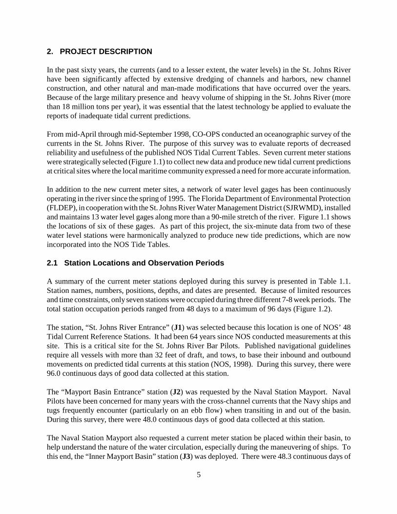
2.1 Station Locations and Observation Periods
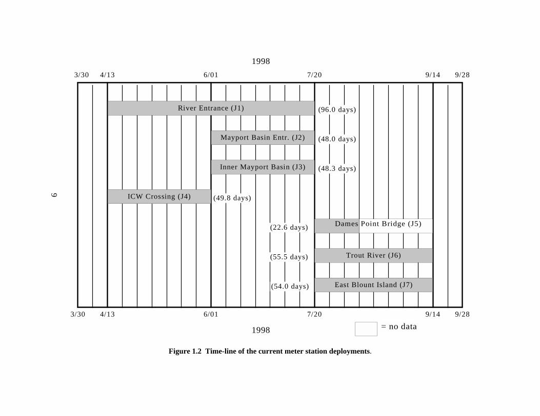
A summary of the current meter stations deployed during this survey is presented in Table 1.1.Station names, numbers, positions, depths, and dates are presented. Because of limited resourcesand time constraints, only seven stations were occupied during three different 7-8 week periods. Thetotal station occupation periods ranged from 48 days to a maximum of 96 days (Figure 1.2).
The station, “St. Johns River Entrance” (J1) was selected because this location is one of NOS’ 48Tidal Current Reference Stations. It had been 64 years since NOS conducted measurements at thissite. This is a critical site for the St. Johns River Bar Pilots. Published navigational guidelinesrequire all vessels with more than 32 feet of draft, and tows, to base their inbound and outboundmovements on predicted tidal currents at this station (NOS, 1998). During this survey, there were96.0 continuous days of good data collected at this station.
The “Mayport Basin Entrance” station (J2) was requested by the Naval Station Mayport. NavalPilots have been concerned for many years with the cross-channel currents that the Navy ships andtugs frequently encounter (particularly on an ebb flow) when transiting in and out of the basin.During this survey, there were 48.0 continuous days of good data collected at this station.
The Naval Station Mayport also requested a current meter station be placed within their basin, tohelp understand the nature of the water circulation, especially during the maneuvering of ships. Tothis end, the “Inner Mayport Basin” station (J3) was deployed. There were 48.3 continuous days of

6
data collected at this station; unfortunately, the current meter was placed too close to the south sideof the basin, and the measured currents were weak and variable. The majority of current speeds weremeasured at less than 1/4 knot, therefore the data were considered unusable.
Table 1.1 St. Johns River current meter station deployment information.
Station Station Name PositionWaterDepth
(MLLW)# DaysData
DeploymentPeriod
J1 St. JohnsRiver Entrance
30b 24.022' N081b 23.154' W
50.8 ft.(15.5 m)
96.0 04/16 - 07/211998
J2 Mayport Basin Entrance 30b 23.820' N081b 23.929' W
43.0 ft.(13.1 m)
48.0 06/03 - 07/211998
J3 Inner Mayport Basin 30b 23.661' N081b 24.403' W
37.1 ft.(11.3 m)
48.3 06/04 - 07/221998
J4 Intracoastal WaterwayIntersection
30b 23.020' N081b 27.519' W
53.8 ft.(16.4 m)
49.8 04/15 - 06/041998
J5 Dames Point Bridge 30b 23.078' N081b 33.276' W
39.0 ft.(11.9 m)
22.6 07/23 - 08/151998
J6 Trout River Cut 30b 23.029' N081b 37.694' W
43.3 ft.(13.2 m)
55.5 07/22 - 09/161998
J7 East Blount Island 30b 23.521' N081b 30.511' W
44.3 ft.(13.5 m)
54.0 07/23 - 09/151998
The “Intracoastal Waterway (ICW) Intersection” station (J4) was one of the highest priority station’srequested by the St. Johns River Bar Pilots. In this area, it was reported that ships frequentlyencounter unpredictable cross-channel currents at various stages of the tide, especially during highstreamflow conditions. In addition, many tugs and tows cross over the river while transiting theICW, further complicating navigation. Prior to this survey, there were no tidal current predictionspublished for this junction of the river. During this survey, 49.8 continuous days of good data werecollected at this station.
The “East Blount Island” station (J7) is another point in the river where it was reported thatunpredictable cross-channel currents are encountered. Before this survey, there were no tidal currentpredictions published for this junction of the river. In addition, the Navy maintains a large storagefacility along the Back River, and they were interested in collecting new information on the currentsin this area. During this survey, 54.0 continuous days of good data were collected at this station.
The “Dames Point Bridge” station (J5) was deployed in an area of particular concern for largevessels transiting the river. Just to the west of this station, there is a sharp turn in the river. Pilotshave reported their ships being “set deep into the bend” on both the flood and the ebb, presumablyfrom cross-channel currents from the Blount Island Channel. In addition, vessels use this area of the

7
channel as a turning basin when using the Blount Island Terminal (NOS, 1998). Due to instrumentbattery failure, only 22.6 days of continuous good data were collected at this station.
The “Trout River Cut” station (J6) was requested by the St. Johns River Bar Pilots because of theeffect of the Trout River on the currents in the main shipping channel. This location is the farthestupriver of the seven stations occupied during this survey. Cross-channel currents are reported to “setacross the channel on both the flood and ebb.” Also, there are many oil terminals in this area, on thewest bank, adding to the pilots’ concerns (NOS, 1998). This location is one of the existing 17subordinate tidal current stations that have been published for many years, however, it had been 40years since NOS conducted new measurements at this site. During this survey, 55.5 continuous daysof good data were collected.
Original survey plans included the deployment of a current meter farther upriver in downtownJacksonville, near the FEC railroad bridge. However, logistical constraints and instrumentationrecovery concerns (reports of bottom debris and bridge construction), prompted a last-minute changein plans, and this current meter was placed at the Dames Point Bridge (station J5).

Figure 1.1 Chartlet of the station locations: current meters and water level gages.
8
Mayport Basin Entr. (J2)
River Entrance (J1)
Inner Mayport Basin (J3)
ICW Crossing (J4)
Dames Point Bridge (J5)
Trout River (J6)
East Blount Island (J7)
(96.0 days)
(48.0 days)
(48.3 days)
(49.8 days)
(22.6 days)
(55.5 days)
(54.0 days)
3/30 4/13 6/01 7/20 9/14
3/30 4/13 6/01 7/20 9/14
9/28
9/28
1998
1998 = no data
Figure 1.2 Time-line of the current meter station deployments.
9

10
Figure 2.1 RDI Workhorse ADCPs used for this survey.
2.2 Instrumentation and Sampling Methods
RD Instruments (RDI) “Workhorse Sentinel” acoustic Doppler current profilers (ADCP) were usedat all of the current meter stations in this survey (Figure 2.1). NOS personnel have deployed dozensof RDI ADCPs in various harbors and estuaries throughout the U.S. for more than 10 years; theseinstruments have a proven reliability and performance. The advent of ADCP technology has enabledNOS to obtain water current data throughout an entire water column with long-term theoreticalaccuracies of approximately 0.02 knots or better (RDI, 1996).
The ADCP computes current velocities throughout a water column by measuring the Doppler shiftof a fixed-frequency sound transmission. Sound scatterers in the water (i.e., plankton, particles, airbubbles) reflect the transmitted sound back to the ADCP in the form of a "backscattered" echo. TheADCPs used in this survey have four acoustic transducer heads equally spaced in the azimuth,known as the “JANUS” configuration. They have four transducers angled at 20 degrees from thehorizontal, and operate at a frequency of 300 kHz.
The most important feature of the ADCP is its ability to remotely measure current profiles, whichare divided into uniform segments called depth cells or "bins" (Figure 2.2). All of the current metersused in this survey were programmed to collect and internally record data at six minute intervals, in1 meter bin lengths throughout the water column.
All of the current meters were deployed on the river bottom in an upward-looking configuration, onplatforms specially designed for instrument protection and leveling: Flotation Technologies TrawlResistant Bottom-Mounts (Figure 2.3) were used. These platforms have the shape of a truncatedpyramid (with the sides angled at approximately 35b from horizontal) built to lift and deflect passingtrawl-type fishing gear. They have overall dimensions of 6 ft. × 6 ft. × 1.7 ft. Their weight in air isapproximately 800 pounds, including the lead ballast.

11
Figure 2.2 Illustration of the profiling ability of a bottom-mounted ADCP.
Figure 2.3 Flotation Technologies, Inc.bottom-mount used for the survey.
The bottom-mounts consist of three main components: a base section made of corrosion resistantaluminum, a recovery pod made of syntactic foam, and a gimbal mechanism made of machinedPVC. The gimbal mechanism orients the ADCP to vertical at bottom slopes of up to 20b. Anacoustic release, housed in the recovery pod, is used for recovering the package. Upon activationof the acoustic release, the recovery pod floats to the surface and the attached line is used to haul thebase onto the ship. One interesting feature of this bottom-mount is that most of the buoyancy issituated on the top half, making it self-righting in “free-fall” when placed in the water at angles upto and even beyond 90 degrees.
Because these bottom-mounts present a relatively low profile, they were all placed directly in themain navigation channel, usually in a deeper section, as determined from the latest hydrographicsurvey sounding data. This provided more representative and useful current measurements than ifthe current meters had been placed on the edge of the navigation channel (as was often necessarywith older technology) to avoid becoming a hazard to navigation.

12
2.3 Data Processing and Quality Control
After the bottom-mounts and current meters were recovered and brought to shore, the raw data weredownloaded from the ADCP’s internal recorder to a laptop PC. The data were then transported toNOAA headquarters in Silver Spring, Maryland, where they were subjected to a set of standard dataquality control (DQC) procedures and thoroughly processed and analyzed. The data were convertedfrom instrument format (binary ADCP) into ASCII engineering units for analysis. Data were thenchecked for time validity, outliers, trends, and noise bursts. Time-series plots were created for eachstation for the various measured parameters.
Each data set was checked for instrument tilts greater than 15 degrees. Any data record that had aninstrument tilt of greater than 15 degrees was not used for analysis. Similarly, if there were anysudden movement of the bottom-mount (illustrated by the tilt sensor, compass, and pressure sensor),the data were scrutinized because a significant movement of the bottom-mount may have occurred.This only occurred in one of the data sets for a relatively short time period.
In order to compute the water depth (from the surface) of each depth cell, some simple computationsare required. First, the distance above the bottom for the center of each depth cell is calculated. Toobtain these, three values are added:
1) the height of the ADCP acoustic heads off of the river bottom;2) the depth cell length;3) the “blanking distance”.
For all of the deployments, these three parameters were fixed at 0.6 m, 1.0 m, and 1.7 m,respectively. To this total, a speed of sound correction of about 0.2m (based on measured watertemperature and estimated conductivity) is added. This gives a “fixed” height above the bottom (forthe first depth cell) of 3.5m for all stations. The second depth cell is 4.5m off of the bottom, and thenth depth cell is (n+2.5) m above the bottom.
Finally, to determine the water depth of each depth cell, the distance above bottom for a given depthcell is subtracted from the total station depth, which was either computed directly from the ADCP’sinternal pressure sensor or estimated from a fathometer and/or bathymetric soundings.
Because of acoustic side lobe interference effects near the river surface, in which the verticallyoriented side lobes combine with the 20-degree main beam, the ADCP data are not assured valid inthe top 6% of the water column (RDI, 1996). Even with this limitation, good data were collectedvery near the surface at each of the seven stations. Depending on the total station depth, theshallowest depth having good data ranged from five to 10 feet below MLLW.

13
-1.0 2.0 5.0 8.0 11.0 14.0 17.0 20.0 23.0 26.0
Distance (nm) From River Mouth
-1.0
0.0
1.0
2.0
3.0
4.0
5.0
6.0
7.0
8.0
9.0
10.0
11.0
12.0
Gre
enw
ich
Inte
rval
(hou
rs)
High Water IntervalLow Water IntervalMaximum FloodMaximum Ebb
Figure 3.1 Time differences, from the river mouth, of two tide and two tidal currentphases. Note that the tidal current phases are for depth cells nearest 15 feet.
3. CURRENTS
Currents in the lower St. Johns River are tidally dominated. Because the river is basically aconstricted channel, the currents are rectilinear (or reversing), in that the water flows alternately inapproximately opposite directions, with a slack water at each reversal of direction. The currents aresemidiurnal, consisting of two flood and two ebb periods each day.
In the 16-mile stretch of river studied in this survey, the currents exhibit mostly progressive wavecharacteristics, meaning that the maximum strengths of flood and ebb occur near the times of highand low water, respectively. This relationship varies along the river (Figure 3.1), depending on thedistance from the mouth of the river, the water depth, and other physical factors. At the riverentrance, the maximum flood and ebb currents occur approximately one hour before the high andlow tides at the river entrance (Figure 3.2). Further upriver, at Dames Point (approximately 10.5miles from the river entrance), the maximum flood and ebb currents precede the times of high andlow water by only about 15-35 minutes (Figure 3.3). Somewhere around 15 to 17 miles from theriver entrance, the flood and ebb strengths occur almost simultaneously with the times of high andlow waters (Figure 3.1).

14
00:00 04:00 08:00 12:00 16:00 20:00
April 28, 1998 (UTC)
-1.0
0.0
1.0
2.0
3.0
4.0
5.0
6.0
7.0
Wat
er L
evel
(fee
t--M
LLW
)
-4.0
-3.0
-2.0
-1.0
0.0
1.0
2.0
3.0
4.0
Spee
d (k
nots
)
water levelcurrent (16.4 ft.)
70 min.
64 min.
Figure 3.2 Phase lag of water level at Mayport D.S. and current at the RiverEntrance (J1). Note that both plots are actual observations, while the timedifferences are mean values.
00:00 04:00 08:00 12:00 16:00 20:00
August 13, 1998 (UTC)
-1.0
0.0
1.0
2.0
3.0
4.0
5.0
Wat
er L
evel
(fee
t--M
LLW
)
-3.0
-2.0
-1.0
0.0
1.0
2.0
3.0
Spee
d (k
nots
)
water levelcurrent (14.4 ft.)
15 min.
35 min.
Figure 3.3 Phase lag of water level and current at Dames Point. Note that bothplots are actual observations, while the time differences are mean values.

15
-1.0 1.0 3.0 5.0 7.0 9.0 11.0 13.0 15.0
Distance (nm) From River Mouth
-2.0
0.0
2.0
4.0
6.0
8.0
10.0
12.0
14.0
Gre
enw
ich
Inte
rval
(hou
rs)
Slack Before FloodMaximum FloodSlack Before EbbMaximum Ebb
2.3 hours difference
2.8 hours difference
2.7 hours difference
2.9 hours difference
J1 J2 J4 J7 J5 J6
Figure 3.4 Time differences, from the river mouth, of the four tidal current phases. Note that all of the values are for depth cells nearest 15 feet.
The progression of the tidal current from the mouth of the river to the Trout River Cut station (J6)is highly linear. In this approximately 16-mile stretch of river, there was a measured time differenceof 2.3 to 2.9 hours (Figure 3.4) for all four of the tidal current phases–slack before flood (SBF),maximum flood current (MFC), slack before ebb (SBE), and maximum ebb current (MEC). Thiscorresponds to an average progression speed of about 5.5 to 7.0 knots, which is importantinformation to mariners when planning for the most efficient times to transit up or down the river.
This direct linear relationship of the tidal current phases along the river was used as a tool to verifyall of the older (1934 and 1958) published tidal current prediction stations. After the final analysis,only one old station was removed from the tidal current tables because the timing of its tidal currentphases fell far outside of the interpolated tidal current phase progression line.
The currents at all of the stations exhibited vertical profiles that are typical of tidal rivers. Figure 3.5shows the deployment-averaged vertical profiles from all of the stations. The current speeds werestrongest near the surface (due to bottom frictional effects), and the down-river stations generally hadstronger currents than the up-river stations.
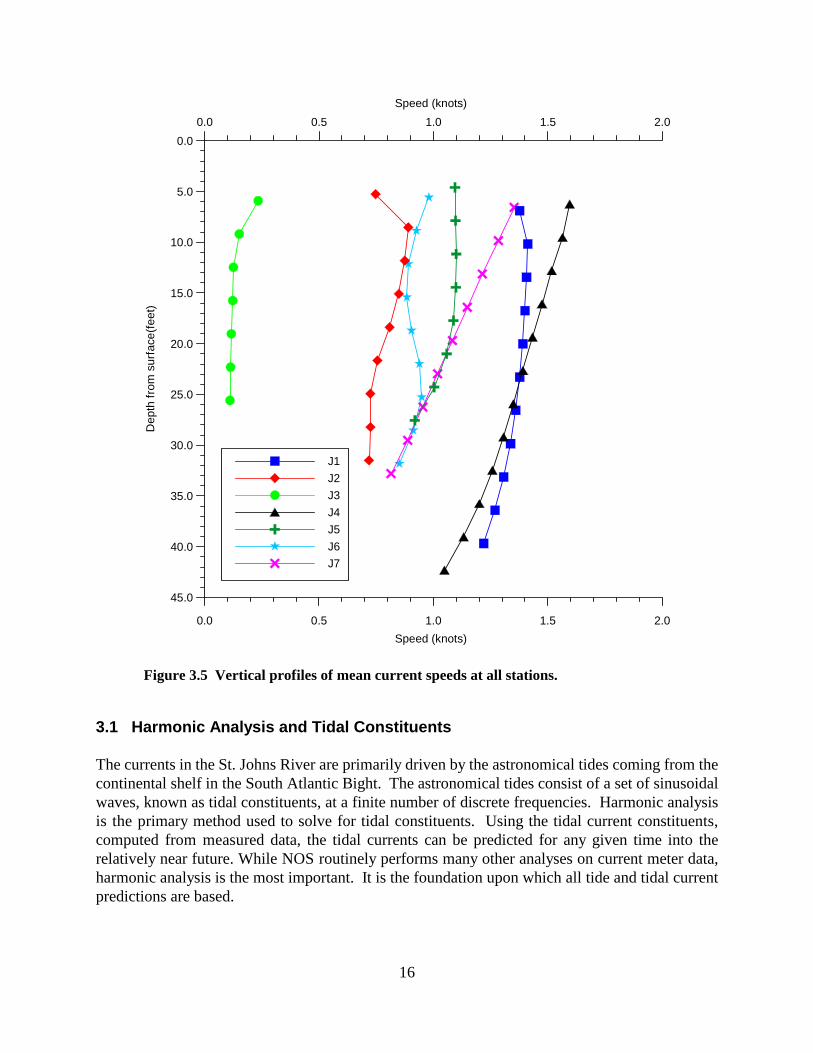
16
0.0 0.5 1.0 1.5 2.0Speed (knots)
45.0
40.0
35.0
30.0
25.0
20.0
15.0
10.0
5.0
0.0D
epth
from
sur
face
(feet
)
0.0 0.5 1.0 1.5 2.0Speed (knots)
J1J2J3J4J5J6J7
Figure 3.5 Vertical profiles of mean current speeds at all stations.
3.1 Harmonic Analysis and Tidal Constituents
The currents in the St. Johns River are primarily driven by the astronomical tides coming from thecontinental shelf in the South Atlantic Bight. The astronomical tides consist of a set of sinusoidalwaves, known as tidal constituents, at a finite number of discrete frequencies. Harmonic analysisis the primary method used to solve for tidal constituents. Using the tidal current constituents,computed from measured data, the tidal currents can be predicted for any given time into therelatively near future. While NOS routinely performs many other analyses on current meter data,harmonic analysis is the most important. It is the foundation upon which all tide and tidal currentpredictions are based.

17
Two different harmonic analysis methods were used on the data collected in this survey. Leastsquares harmonic analysis (Harris et al., 1963) was performed on the five stations that had 48 daysor more of data, and Fourier harmonic analysis (Dennis and Long, 1971) was performed on theDames Point station (J5), which collected only 23 days of data. The five principal tidal currentharmonic constituents computed for the six stations are listed in Table 3.1. They are listed in orderfrom down-river to up-river, with three depths each. In general, all of the epochs (phases) increaseupriver, which is typical for a tidal river.
Table 3.1 Principal tidal current constituents: amplitudes (along-channel in knots) and epochs(kappas) of the five most significant tidal current constituents. Stations are listed from down-riverto up-river.
StationDepth(ft.)
M2 S2 N2 K1 O1
Amp. Epoch Amp. Epoch Amp. Epoch Amp. Epoch Amp. Epoch
J1 9.8 2.02 195.6 0.24 215.1 0.42 168.1 0.21 76.0 0.17 93.7
J1 16.4 2.01 194.1 0.24 216.7 0.40 167.6 0.21 74.4 0.17 91.5
J1 29.5 1.91 191.2 0.23 220.1 0.38 167.7 0.20 70.6 0.17 89.7
J2 8.5 1.25 195.0 0.09 176.5 0.18 160.9 0.15 73.6 0.05 92.8
J2 15.1 1.22 194.6 0.08 189.1 0.18 163.9 0.15 69.6 0.07 91.7
J2 31.5 0.91 205.7 0.08 197.8 0.13 174.2 0.12 81.0 0.10 109.7
J4 9.5 2.10 207.2 0.28 220.9 0.43 173.5 0.27 64.4 0.19 93.6
J4 16.1 2.03 205.3 0.28 221.3 0.42 174.2 0.26 60.3 0.19 95.4
J4 29.2 1.81 200.4 0.25 220.1 0.39 174.9 0.23 56.1 0.18 90.5
J7 6.6 1.85 230.1 0.21 253.5 0.29 211.7 0.18 129.8 0.12 121.3
J7 16.4 1.58 225.5 0.18 247.4 0.25 204.4 0.16 125.1 0.12 123.2
J7 29.5 1.22 222.6 0.16 248.9 0.22 201.8 0.13 121.8 0.08 130.4
J5 4.6 1.54 245.0 0.17 266.1 0.30 233.7 0.15 113.8 0.07 149.3
J5 14.4 1.60 240.6 0.19 267.3 0.31 227.0 0.14 115.3 0.06 134.9
J5 27.6 1.30 244.6 0.19 280.7 0.25 225.4 0.19 130.5 0.12 144.5
J6 5.6 1.40 269.2 0.14 294.0 0.19 253.5 0.14 150.5 0.12 139.4
J6 15.4 1.24 269.1 0.14 299.0 0.20 255.9 0.13 150.7 0.10 149.5
J6 31.8 1.17 266.3 0.12 299.1 0.18 253.8 0.12 149.4 0.08 153.2
The least squares harmonic analysis directly solves for up to 175 different tidal current constituents,depending on the length of the data set. For the data in this survey, 23 tidal current constituents werecomputed. Fourier harmonic analysis (29-day) solves for 25 tidal current constituents: eleven tidal

18
current constituents are directly computed, while 14 others are derived using standard amplitude andphase relationships from equilibrium theory.
The M2 constituent is the major semidiurnal lunar constituent. It is due to the direct tide producingforce of the moon and has a period of 12.42 hours. S2 is the major semidiurnal solar constituent dueto the sun; it has a period of 12.00 hours. The interaction of the two constituents going in and outof phase with each other causes the spring/neap cycles.
3.2 St. Johns River Entrance (J1)
Prior to this survey, the St. Johns River Entrance was an NOS Reference Station for only17 subordinate tidal current stations; the previous predictions at this Reference Station had beenbased on two 15-day current pole observations collected in 1934. The new data collected at thisstation are now being used to compute all of the published NOS tidal current predictions in the St.Johns River. Starting with the 1999 edition of the NOS Tidal Current Tables, a total of 55subordinate tidal current stations (including multiple depths at 20 individual sites) will be referencedto the St. Johns River Entrance station. Appendix B contains the year 2000 tidal current predictions(Table 1 and Table 2) for the St. Johns River. In addition to the new data collected during thissurvey, there were older, archived data that were previously unpublished. These data were revisited,and where appropriate, they were fully processed and analyzed.
The new Reference Station was deployed approximately 270 yards to the west of the publishedposition of the 1934 station, allowing for a direct inter-comparison of the two data sets. Figure 3.6is a 16-hour time-series plot comparing the tidal current predictions based on the 1934 data with thetidal current predictions based on the new 1998 data. The most apparent difference between the twosets of predictions is seen in the phase of the currents: all four phases (SBE, MEC, SBF, MFC) ofthe new tidal current predictions occur earlier than the old tidal current predictions, by as much asalmost an hour. Over the past 64 years, there have been numerous bathymetric and hydrologicalchanges in the river, having a pronounced effect on the amplitude and phase of the currents.
The new predicted maximum flood speeds are slightly stronger than the old predicted maximumflood speeds, while the new predicted maximum ebb speeds are slightly weaker than the oldpredicted maximum ebb speeds. The smaller ebb speeds may be a result of the considerabledeepening and widening of the river over the past 60-plus years. Currents (especially ebb currents)in a tidal river such as the St. Johns River will generally decrease when the cross-sectional area(depth and width) is increased, assuming the overall discharge stays fairly constant during that time(Pond and Pickard, 1983).
The maximum current speed observed during the 96.0 day measurement period was 3.43 knotstoward 264.3 degrees, which is in the flood direction. This speed was measured at a depth of 9.8 feeton May 25, 1998, on the day of a new moon. Figure 3.7 is a velocity scatter diagram of the currentsat a depth of 16.4 feet. The effect of the Mayport Basin is clearly seen here during the ebb current;in the northeast quadrant, there is a small divergence of the flow, especially at ebb speeds greaterthan about 1.5 knots.

19
-3.0
-2.0
-1.0
0.0
1.0
2.0
3.0
Spee
d (k
nots
)
1934-based1998-based
FLOOD
EBB
SBF(56 minutes)
SBE(16 minutes)
Max Ebb(20 minutes)
Max Flood(39 minutes)
-3.0
-2.0
-1.0
0.0
1.0
2.0
3.0
Spee
d (k
nots
)
Figure 3.6 Comparison of the 1934-based and the 1998-based tidal currentpredictions at the River Entrance (J1).
mean north component = 0.04 knotsmean east component = 0.12 knots
-4.0 -3.0 -2.0 -1.0 0.0 1.0 2.0 3.0 4.0East component (knots)
-4.0
-3.0
-2.0
-1.0
0.0
1.0
2.0
3.0
4.0
Nor
th c
ompo
nent
(kno
ts)
Figure 3.7 Velocity scatter diagram for theRiver Entrance (J1), 16.4 ft. depth.
Figure 3.8 Speed-direction scatter plotfor the River Entrance (J1), 9.8 ft. depth.

20
standard deviation = 0.23 knots
-1.0
0.0
1.0
8-Jul 9-Jul 10-Jul 11-Jul 12-Jul 13-Jul 14-Jul 15-Jul
1998 Days (UTC)
Res
idua
l Spe
ed (k
nots
)
-5.0
-4.0
-3.0
-2.0
-1.0
0.0
1.0
2.0
3.0
4.0
Spee
d (k
nots
)
observedpredictedresidual
(16.4 ft. depth)
Figure 3.9 Observed, predicted, and residual current (along-channel--262bbbb) at theRiver Entrance (J1) during a seven day period. Note that the residual standarddeviation value is for the entire 96.0-day deployment period.
Figure 3.8 is a speed-direction scatter plot of the currents at a depth of 9.8 feet. This is a goodillustration of the bipolar, rectilinear nature of the currents in the river. The ebb current (meandirection of 81b True) is not as “tight” as the flood current (mean direction of 262b True), again dueto the draining of the Mayport Basin during the stronger ebb flows. The effect of the jetties in thisarea is to constrict the direction of the current.
A seven-day time-series plot representing the measured currents, astronomical predictions, andresidual currents (all along-channel at 16.4 ft. depth) is presented in Figure 3.9. The tidal currentconstituents, obtained by least-squares harmonic analysis, were used to predict the tidal current forthe 96.0-day measurement period. These values were then subtracted from the observed current toobtain the residual current.
Analysis of the residual current at the 16.4 ft. depth reveals that the standard deviation for themeasurement period is 0.23 knots. The standard deviation is a direct measure of the observedvariability in a time-series. When applied to the residual current, it is a good method to gage theproportion of nontidal energy in the total current. The astronomical constituents accounted for morethan 97% of the total variance, with the M2 constituent comprising over 90% of the total variancealone. The remaining 3% of the variance is due to meteorological and hydrological forces, such asweather fronts, offshore events, and streamflow. Results for the other depths are similar.

21
3.3 Mayport Basin Entrance (J2)
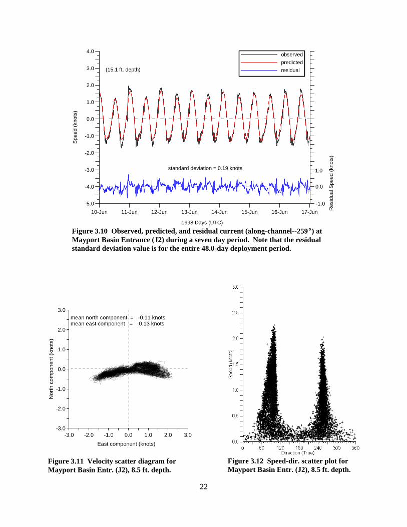
The Mayport Basin Entrance is a new station for NOS, so there are no prior data at this site to makecomparisons. A seven-day time-series plot representing the measured currents, astronomicalpredictions, and residual currents (all along-channel at 15.1 ft. depth) is presented in Figure 3.10.The tidal current constituents were obtained by least-squares harmonic analysis, and used to computethe astronomical tidal current for the 48.0-day measurement period. These values were thensubtracted from the observed current to obtain the residual current. This procedure was performedon data at three different depths: 8.5 ft., 15.1 ft., and 31.5 ft.
Analysis of the residual current at the 15.1 ft. depth reveals that the standard deviation for themeasurement period is 0.19 knots. The astronomical constituents account for 96% of the totalvariance, with the M2 constituent comprising over 90% of the total variance alone. The remaining4% of the variance is due to meteorological and hydrological forces. Results for the other depths aresimilar.
The maximum current speed observed during the measurement period was 2.53 knots toward103.4 degrees, which is in the ebb direction. This speed was measured at a depth of 5.2 feet onJune 10, 1998, on the day of a full moon. The current in the upper five to 12 feet of the watercolumn exhibits a significant cross-channel flow, cutting across the Mayport channel axis at abouta 25b to 30b angle, especially during ebbing currents greater than about 1.8 knots (Figure 3.11). Infact, the vast majority of the strongest currents (from 1.8 knots to 2.2 knots) observed at this stationoccurred in the upper five to 12 feet, during ebb flow, at angles across the main channel.
The current below about 12 feet showed some cross-channel flow during ebb conditions, but not tothe same extent as the surface water. The ebb current strength decreased with depth, and the angleof the cross-channel flow was not as extreme towards the deeper sections. The strongest currentsbelow 12 feet were from about 1.4 knots to 1.7 knots, mostly in a flood direction, in-line with thechannel.
Figure 3.12 is a speed-direction scatter plot of the currents at a depth of 8.5 feet; it illustrates therelative flood and ebb distribution. This figure shows that the ebb current (mean direction of93b True) is slightly stronger than the flood current (mean direction of 255b True), and that the twoaxes are 162b apart, owing to the cross-channel flow at this depth.
22
Figure 3.12 Speed-dir. scatter plot forMayport Basin Entr. (J2), 8.5 ft. depth.
mean north component = -0.11 knotsmean east component = 0.13 knots
-3.0 -2.0 -1.0 0.0 1.0 2.0 3.0East component (knots)
-3.0
-2.0
-1.0
0.0
1.0
2.0
3.0
Nor
th c
ompo
nent
(kno
ts)
Figure 3.11 Velocity scatter diagram forMayport Basin Entr. (J2), 8.5 ft. depth.
standard deviation = 0.19 knots
-1.0
0.0
1.0
10-Jun 11-Jun 12-Jun 13-Jun 14-Jun 15-Jun 16-Jun 17-Jun
1998 Days (UTC)
Res
idua
l Spe
ed (k
nots
)
-5.0
-4.0
-3.0
-2.0
-1.0
0.0
1.0
2.0
3.0
4.0
Spee
d (k
nots
)
observedpredictedresidual(15.1 ft. depth)
Figure 3.10 Observed, predicted, and residual current (along-channel--259bbbb) atMayport Basin Entrance (J2) during a seven day period. Note that the residualstandard deviation value is for the entire 48.0-day deployment period.

23
Figure 3.14 Speed-Dir. scatter plot forInner Mayport Basin (J3), 9.2 ft. depth.
mean north component = -0.03 knotsmean east component = -0.04 knots
-3.0 -2.0 -1.0 0.0 1.0 2.0 3.0East component (knots)
-3.0
-2.0
-1.0
0.0
1.0
2.0
3.0
Nor
th c
ompo
nent
(kno
ts)
Figure 3.13 Velocity scatter diagram forInner Mayport Basin (J3), 5.9 ft. depth.
3.4 Inner Mayport Basin (J3)
Figure 3.13 is a velocity scatter diagram of the currents at a depth of 5.9 feet, and Figure 3.14 is aspeed-direction scatter plot of the currents at a depth of 9.2 feet. Both figures clearly show theextremely slow currents measured at this station. These weak currents were most likely a result ofthe current meter’s position–it was placed too close to the south side of the basin, very near theNaval pier known as “foxtrot” pier. If the station had been positioned just 100 yards to the north,the measured currents most likely would have been more substantial. Because of the very lowobserved currents at this station, the data were considered unusable, and no harmonic analyses wereperformed or astronomical predictions computed. The NOS standard is that any current less than1/4 knot is considered weak and variable.
The maximum current speed observed during the measurement period was 0.91 knots toward 247.0degrees, which is in the flood direction. This speed was measured at a depth of 5.9 feet onJune 10, 1998, on the day of a full moon. However, it was an anomalous value; less than 10% ofthe measurements at this depth exceeded 1/2 knot. All other depths showed even slower speeds: asthe depth increased, the observed current decreased markedly. The current at 9.2 feet exceeded 1/2knot only eight times out of the more than 11,000 six-minute observations, and exceeded 1/4 knotonly 13% of the 48.3-day measurement period.

24
3.5 Intracoastal Waterway Intersection (J4)
The Intracoastal Waterway (ICW) Intersection is a new station for NOS, so there are no prior dataat this site to make comparisons. A seven-day time-series plot representing the measured currents,astronomical predictions, and residual currents (all along-channel at 16.1 ft. depth) is presented inFigure 3.15. The tidal current constituents were obtained by least-squares harmonic analysis, andused to compute the astronomical tidal current for the 49.8-day measurement period. These valueswere then subtracted from the observed current to obtain the residual current. This procedure wasperformed on data at three different depths: 9.5 ft., 16.1 ft., and 29.2 ft.
Analysis of the residual current at the 16.1 ft. depth reveals that the standard deviation for themeasurement period is 0.25 knots. The astronomical constituents account for more than 97% of thetotal variance, with the M2 constituent comprising almost 90% of the total variance alone. Theremaining 3% of the variance is due to meteorological and hydrological forces. Results for the otherdepths are similar.
The ICW crosses the main channel of the St. Johns River at about a 45b angle from the north; while,from the south, it enters almost parallel to the main channel. Because of the influence of the ICW,the current in the upper six to 23 feet of the water column exhibits a significant cross-channel flow,mainly early in the ebb cycle, when the current is between about 0.5 knots to 1.3 knots. During theseconditions, the water from the ICW (flowing out from the south) causes a cross-channel flow atabout 30b to 40b across the main channel (Figure 3.16). When the ebbing current in the upper23 feet becomes greater than about 1.5 knots, the direction of the flow comes in-line with the mainchannel. The current below about 23 ft. depth showed some cross-channel flow, but not nearly tothe same extent as the surface water.
The maximum current speed observed during the measurement period was 3.79 knots toward132.6 degrees, which is in the ebb direction. This speed was measured at a depth of 6.2 feet onApril 27, 1998, one day after a new moon. The flood currents are significantly weaker than the ebbcurrents at this station: at 9.5 ft., the maximum flood currents (mean direction of 293b True) averageonly 1.6 knots, while the maximum ebb currents (mean direction of 125b True) average 2.6 knots(Figure 3.17). Also, at 16.1 ft., the maximum flood currents average only 1.6 knots, while themaximum ebb currents average 2.4 knots.
In the upper 23 ft., the current at this station rotates clockwise during a given tidal cycle; the ebbcurrent will start flowing toward about 80b to 90b until the speed reaches about 1.3 knots to1.5 knots, when the direction of the current will rapidly change to about 120b to 130b, in-line withthe main channel. The current then remains in this state, slows to a minimum current, then quicklyturns to a flood toward about 300b. Because of the influence of the ICW, the slack-before-ebb at thisstation is relatively high; it is usually greater than 1/3 knot, while the slack-before-flood is almostalways less than 1/4 knot.

25
Figure 3.17 Speed-Dir. scatter plot forI.C.W. Intersection (J4), 9.5 ft. depth.
mean north component = -0.10 knotsmean east component = 0.32 knots
-4.0 -3.0 -2.0 -1.0 0.0 1.0 2.0 3.0 4.0East component (knots)
-4.0
-3.0
-2.0
-1.0
0.0
1.0
2.0
3.0
4.0
Nor
th c
ompo
nent
(kno
ts)
Figure 3.16 Velocity scatter diagram forI.C.W. Intersection (J4), 16.1 ft. depth.
standard deviation = 0.25 knots
-1.0
0.0
1.0
1-May 2-May 3-May 4-May 5-May 6-May 7-May 8-May
1998 Days (UTC)
Res
idua
l Spe
ed (k
nots
)
-5.0
-4.0
-3.0
-2.0
-1.0
0.0
1.0
2.0
3.0
4.0
Spee
d (k
nots
)
observedpredictedresidual(16.1 ft. depth)
Figure 3.15 Observed, predicted, and residual current (along-channel--293bbbb) at theI.C.W. Intersection (J4) during a seven day period. Note that the residual standarddeviation value is for the entire 49.8-day deployment period.
26
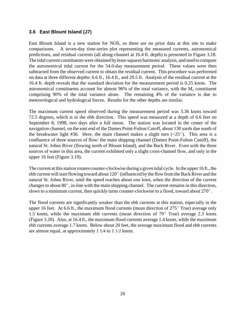
3.6 East Blount Island (J7)
East Blount Island is a new station for NOS, so there are no prior data at this site to makecomparisons. A seven-day time-series plot representing the measured currents, astronomicalpredictions, and residual currents (all along-channel at 16.4 ft. depth) is presented in Figure 3.18.The tidal current constituents were obtained by least-squares harmonic analysis, and used to computethe astronomical tidal current for the 54.0-day measurement period. These values were thensubtracted from the observed current to obtain the residual current. This procedure was performedon data at three different depths: 6.6 ft., 16.4 ft., and 29.5 ft. Analysis of the residual current at the16.4 ft. depth reveals that the standard deviation for the measurement period is 0.25 knots. Theastronomical constituents account for almost 96% of the total variance, with the M2 constituentcomprising 90% of the total variance alone. The remaining 4% of the variance is due tometeorological and hydrological forces. Results for the other depths are similar.
The maximum current speed observed during the measurement period was 3.36 knots toward72.5 degrees, which is in the ebb direction. This speed was measured at a depth of 6.6 feet onSeptember 8, 1998, two days after a full moon. The station was located in the center of thenavigation channel, on the east end of the Dames Point-Fulton Cutoff, about 130 yards due south ofthe breakwater light #36. Here, the main channel makes a slight turn (~25b). This area is aconfluence of three sources of flow: the main shipping channel (Dames Point-Fulton Cutoff), thenatural St. Johns River (flowing north of Blount Island), and the Back River. Even with the threesources of water in this area, the current exhibited only a slight cross-channel flow, and only in theupper 16 feet (Figure 3.19).
The current at this station rotates counter-clockwise during a given tidal cycle. In the upper 16 ft., theebb current will start flowing toward about 120b (influenced by the flow from the Back River and thenatural St. Johns River, until the speed reaches about one knot, when the direction of the currentchanges to about 80b, in-line with the main shipping channel. The current remains in this direction,slows to a minimum current, then quickly turns counter-clockwise to a flood, toward about 270b.
The flood currents are significantly weaker than the ebb currents at this station, especially in theupper 16 feet. At 6.6 ft., the maximum flood currents (mean direction of 275b True) average only1.5 knots, while the maximum ebb currents (mean direction of 79b True) average 2.3 knots(Figure 3.20). Also, at 16.4 ft., the maximum flood currents average 1.4 knots, while the maximumebb currents average 1.7 knots. Below about 20 feet, the average maximum flood and ebb currentsare almost equal, at approximately 1 1/4 to 1 1/2 knots.

27
standard deviation = 0.25 knots
-1.0
0.0
1.0
5-Aug 6-Aug 7-Aug 8-Aug 9-Aug 10-Aug 11-Aug 12-Aug
1998 Days (UTC)
Res
idua
l Spe
ed (k
nots
)
-5.0
-4.0
-3.0
-2.0
-1.0
0.0
1.0
2.0
3.0
4.0
Spee
d (k
nots
)
observedpredictedresidual(16.4 ft. depth)
Figure 3.18 Observed, predicted, and residual current (along-channel–270bbbb) atEast Blount Island (J7) during a seven day period. Note that the residual standarddeviation value is for the entire 54.0-day deployment period.
Figure 3.20 Speed-Dir. scatter plot forEast Blount Island (J7), 6.6 ft. depth.
-3.0 -2.0 -1.0 0.0 1.0 2.0 3.0East component (knots)
-3.0
-2.0
-1.0
0.0
1.0
2.0
3.0
Nor
th c
ompo
nent
(kno
ts)
mean north component = 0.09 knotsmean east component = 0.27 knots
Figure 3.19 Velocity scatter diagram forEast Blount Island (J7), 9.8 ft. depth.

28
3.7 Dames Point Bridge (J5)
Dames Point Bridge is a new station for NOS, so there are no prior data at this site to makecomparisons. A seven-day time-series plot representing the measured currents, astronomicalpredictions, and residual currents (all along-channel at 14.4 ft. depth) is presented in Figure 3.21.The tidal current constituents were obtained by 15-day Fourier harmonic analysis, and used tocompute the astronomical tidal current for the 22.6-day measurement period. These values were thensubtracted from the observed current to obtain the residual current. This procedure was performedon data at three different depths: 4.6 ft., 14.4 ft., and 27.6 ft. Analysis of the residual current at the14.4 ft. depth reveals that the standard deviation for the measurement period is 0.28 knots.
Only 22.6 days of data were collected at this station, so a 15-day Fourier harmonic analysis wasperformed, as opposed to a 29-day Fourier harmonic analysis or a least-squares harmonic analysis.The main difference in the 15-day Fourier harmonic analysis is that the N2 tidal constituent isinferred from the M2 tidal constituent, and 14 other tidal constituents are inferred (from equilibriumtheory) rather than computed directly as with the least-squares harmonic analysis. This explains thehighest prediction error (based on the residual standard deviation) of any of the stations in this survey.
The maximum current speed observed at this station during the measurement period was 2.56 knotstoward 85.1 degrees, which is in the ebb direction. This speed was measured at a depth of 4.6 feeton July 25, 1998, two days after a new moon. The station was located in the center of the navigationchannel, on the west end of the Dames Point-Fulton Cutoff, about 200 yards due east of the DamesPoint bridge. Here, the Blount Island channel enters the main shipping channel from the north. Evenwith this confluence, the current exhibited only a slight cross-channel flow, and only in the upper14 feet, late in the flood cycle (Figure 3.22).
In the upper 14 ft., the current rotates counter-clockwise during a given tidal cycle; the ebb currentwill start flowing toward about 70b to 80b, in-line with the main shipping channel. The currentremains in this direction, slows to a minimum current, then turns counter-clockwise to a flood,toward about 280b. The flood direction remains at about 280b, until late in the flood cycle, whenthe current slows to less than one knot. The current then turns to about 230b to 260b, beinginfluenced by the inflowing water of the Blount Island channel to the north.
The flood currents are significantly weaker than the ebb currents at this station. At 4.6 ft., themaximum flood currents (mean direction of 254b True) average only 1.2 knots, while the maximumebb currents (mean direction of 80b True) average 1.9 knots (Figure 3.23). Also, at 14.4 ft., themaximum flood currents average 1.4 knots, while the maximum ebb currents average 1.8 knots.

29
standard deviation = 0.28 knots
-1.0
0.0
1.0
5-Aug 6-Aug 7-Aug 8-Aug 9-Aug 10-Aug 11-Aug 12-Aug
1998 Days (UTC)
Res
idua
l Spe
ed (k
nots
)
-5.0
-4.0
-3.0
-2.0
-1.0
0.0
1.0
2.0
3.0
4.0
Spee
d (k
nots
)
observedpredictedresidual(14.4 ft. depth)
Figure 3.21 Observed, predicted, and residual current (along-channel–257bbbb) atDames Point Bridge (J5) during a seven day period. Note that the residualstandard deviation value is for the entire 22.6-day deployment period.
Figure 3.23 Speed-Dir. scatter plot forDames Point Bridge (J5), 4.6 ft. depth.
-3.0 -2.0 -1.0 0.0 1.0 2.0 3.0East component (knots)
-3.0
-2.0
-1.0
0.0
1.0
2.0
3.0
Nor
th c
ompo
nent
(kno
ts)
mean north component = 0.07 knotsmean east component = 0.31 knots
Figure 3.22 Velocity scatter diagram forDames Point Bridge (J5), 7.9 ft. depth.

30
FLOOD
EBB
SBF(58 minutes)
SBE(34 minutes)
Max Ebb(58 minutes)
Max Flood(41 minutes)
-2.0
-1.0
0.0
1.0
2.0
Spee
d (k
nots
)
1958-based1998-based
-2.0
-1.0
0.0
1.0
2.0
Spee
d (k
nots
)
Figure 3.24 Comparison of the 1958-based and the 1998-based tidal currentpredictions at Trout River Cut (J6).
3.8 Trout River Cut (J6)
Prior to this survey, the Trout River Cut station was known as “Phoenix Park.” This was an NOSsubordinate station, based on the St. Johns River Entrance reference station. The previouspredictions at this station had been based on five days of observations collected in 1958. The newdata collected at this station are now being used in the NOS Tidal Current Tables (Appendix B). Thenew current meter at this site was located about 240 yards to the north of the published position ofthe 1958 station, so, a direct inter-comparison of the two data sets is possible.
Figure 3.24 is a 16-hour time-series plot comparing the tidal current predictions based on the 1958data and the new 1998 data. The most apparent difference between the two sets of predictions isseen in the phase of the currents: all four phases (SBE, MEC, SBF, MFC) of the new tidal currentpredictions occur earlier than the old tidal current predictions, from at least a half-hour to as muchas an hour. The new predicted maximum flood speeds are about the same as the old predictedmaximum flood speeds, while the new predicted maximum ebb speeds are stronger than the oldpredicted maximum ebb by about 25%. As with the St. Johns River Entrance station, numerousbathymetric and hydrological changes have occurred in this area over the past 40 years, causingchanges to the amplitude and phase of the currents.

31
A seven-day time-series plot representing the measured currents, astronomical predictions, andresidual currents (all along-channel at 15.4 ft. depth) is presented in Figure 3.25. The tidal currentconstituents, obtained by least-squares harmonic analysis, were used to predict the tidal current forthe 55.5-day measurement period. These values were then subtracted from the observed current toobtain the residual current.
Analysis of the residual current at the 15.4 ft. depth reveals that the standard deviation for themeasurement period is 0.19 knots. The astronomical constituents account for almost 96% of thetotal variance, with the M2 constituent comprising more than 90% of the total variance alone. Theremaining 4% of the variance is due to meteorological and hydrological forces. Results for the otherdepths are similar.
The station was located in the center of the navigation channel, on the south end of the Trout RiverCut Range, about 150 yards from the navigational buoys “67" and “68". Here, the Trout River entersthe main shipping channel from the west. The current at this station generally did not exhibit anycross-channel flow, even with the proximity of the Trout River. This may have been a function ofthe particular position of the instrument. Had the station been positioned further to the north, theremay have been a significant cross-channel flow observed.
The maximum current speed observed during the 55.5-day measurement period was 2.18 knotstoward 15.4 degrees, which is in the ebb direction. This speed was measured at a depth of 8.9 feeton September 8, 1998, two days after a full moon. Figure 3.26 is a velocity scatter diagram of thecurrents at a depth of 8.9 feet. It shows that, overall, the flood currents are slightly weaker than theebb currents at this station, and there is little cross-channel flow.
Figure 3.27 is a speed-direction scatter plot of the currents at a depth of 5.6 feet. This againillustrates the rectilinear nature of the currents at this station. At 5.6 ft., the maximum flood currents(mean direction of 193b True) average 1.3 knots, while the maximum ebb currents (mean directionof 005b True) average 1.5 knots. Also, at 15.4 ft., the maximum flood currents average 1.1 knots,while the maximum ebb currents average 1.3 knots (Appendix B).

32
standard deviation = 0.19 knots
-1.0
0.0
1.0
5-Aug 6-Aug 7-Aug 8-Aug 9-Aug 10-Aug 11-Aug 12-Aug
1998 Days (UTC)
Res
idua
l Spe
ed (k
nots
)
-5.0
-4.0
-3.0
-2.0
-1.0
0.0
1.0
2.0
3.0
4.0
Spee
d (k
nots
)
observedpredictedresidual(15.4 ft. depth)
Figure 3.25 Observed, predicted, and residual current (along-channel–191bbbb) atTrout River Cut (J6) during a seven day period. Note that the residual standarddeviation value is for the entire 55.5-day deployment period.
-3.0 -2.0 -1.0 0.0 1.0 2.0 3.0East component (knots)
-3.0
-2.0
-1.0
0.0
1.0
2.0
3.0
Nor
th c
ompo
nent
(kno
ts)
mean north component = 0.06 knotsmean east component = 0.00 knots
Figure 3.26 Velocity scatter diagram forTrout River Cut (J6), 8.9 ft. depth.
Figure 3.27 Speed-Dir. scatter plot forTrout River Cut (J6), 5.6 ft. depth.

33
31-Jul 1-Aug 2-Aug 3-Aug 4-Aug 5-Aug 6-Aug 7-Aug
1998 Days (UTC)
0
5
10
15
20
25
Spee
d (k
nots
)
0
100
200
300
400
Dire
ctio
n (T
rue)
SpeedGust
Figure 4.1 Wind speed, gust, and direction at Mayport during an early August1998 storm event. Note that the wind direction is the direction the wind is from.
4. RESPONSE OF THE CURRENTS AND WATER LEVELS TO A STORM EVENT
Prevailing winds in the lower St. Johns River basin are northeasterly in the fall and winter months,and southwesterly in spring and summer. The strongest winds generally occur in February andMarch, while lighter winds generally occur in July and August. The greatest rainfall, mostly in theform of local thundershowers, occurs during the summer months in the lower SJR basin. Rainfallof 1 inch or more in 24 hours normally occurs about fourteen times a year, and very infrequentlyheavy rains, associated with tropical storms, reach amounts of several inches with durations of morethan 24 hours. Winter is the dry season, having the least rainfall. River flow is seasonal, generallyfollowing the seasonal rain patterns, with higher flows occurring in the late summer to early fall, andthe lower flows occurring in the winter months (NOAA, 1998).
Throughout the lower St. Johns River, more than 80% of the total river flow is attributed to tidalforces (NOAA, 1985). However, during storm events, the tides can be overcome by nontidal factorssuch as wind, rain, and streamflow. Persistent winds from the north will cause a marked elevationof the water levels, a significant increase of the flood current speeds, and lengthening of the floodcurrent duration. Winds from the south will have the opposite effect. Wind setup occurs atsustained wind speeds of greater than about 7 knots.
From August 2-4, a persistent wind blew from the north at 10-15 knots for more than 48 hours,gusting consistently near 20 knots (Figure 4.1). While not an extreme storm, the persistent directionand speed of the wind caused a significant setup in the water levels and affected the currentssubstantially (Figure 4.2, panels A and B).

34
In addition to the steady wind, there was significant rainfall associated with this storm. This isreflected in the streamflow from a USGS gaging station in Pablo Creek, just south of the SJR, nearMayport (Figure 4.2, panel C). It shows that a sharp rise in the streamflow occurred in less thaneight hours, late on August 1, peaking at over 530 cfs. This turned out to be the annual peak at thisgaging station for 1998. The mean daily flow for this station is approximately 50 cfs.
Prior to the storm, the observed water levels throughout the lower SJR were all running at or justunder predicted tides. The observed water levels at Dames Point were lower than the predicted tideby about 0.1 ft. to 1 ft. (Figure 4.2, panel A). Late on August 1, the water level began respondingto the persistent northerly winds and increased streamflow, and rose to about 1 ft. over the predictedtide. The water levels continued in this state for about 2 1/2 days, until late on August 4, when theybegan to slowly fall back down in line with the predicted tide.
Observed currents at the two operating current meters (Trout River and East Blount Island) were ingood agreement with tidal current predictions, prior to the storm. Late on August 1, the observedcurrent at East Blount Island began responding to the persistent northerly winds (Figure 4.2,panel B). The ebb current speeds were reduced by as much as 3/4 knot, while the ebb currentduration was reduced by about 1 1/2 hours. The flood current speeds were increased by as much as1 knot, while the flood current duration was increased by about 1 1/2 to 2 hours. The currents at thisstation were affected for about 1 1/2 days, until mid-day on August 3, when they quickly returnedback to a normal tidal state.
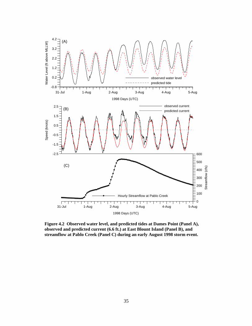
35
31-Jul 1-Aug 2-Aug 3-Aug 4-Aug 5-Aug
1998 Days (UTC)
-0.8
0.2
1.2
2.2
3.2
4.2
Wat
er L
evel
(ft a
bove
MLL
W)
observed water levelpredicted tide
(A)
31-Jul 1-Aug 2-Aug 3-Aug 4-Aug 5-Aug
1998 Days (UTC)
0
100
200
300
400
500
600
Stre
amflo
w (c
fs)
-2.5
-1.5
-0.5
0.5
1.5
2.5
Spee
d (k
nots
)
observed currentpredicted current
Hourly Streamflow at Pablo Creek
(B)
(C)
Figure 4.2 Observed water level, and predicted tides at Dames Point (Panel A),observed and predicted current (6.6 ft.) at East Blount Island (Panel B), andstreamflow at Pablo Creek (Panel C) during an early August 1998 storm event.

36

37
5. SUMMARY
The National Ocean Service’s Center for Operational Oceanographic Products and Servicesconducted an oceanographic survey of the currents in the St. Johns River, Florida from mid Aprilto mid September, 1998. The main goal of this survey was to collect new measurements of thecurrents in as many sites as feasible in the St. Johns River to update the published tidal currentpredictions. New measurements of the currents in the St. Johns River had not been collected sincesurveys in the 1930s and 1950s. Over the decades, the currents have been affected by extensivedredging of channels, new harbor and channel construction, and other natural and man-mademodifications. The large military presence and shipping industry in the St. Johns River require thataccurate tidal current predictions be available.
From the river’s entrance near the Mayport Naval Station to the Trout River Cut, seven new currentmeter stations were occupied throughout a sixteen-mile stretch of river, where the local communityexpressed a need for more accurate information. The results of this survey have led to the generationof new, more accurate tidal current predictions, which will serve to increase the safety and efficiencyof navigation and commerce in the SJR system. Because of this survey, 18 new tidal currentprediction stations (six stations with three depths each) were added to the Tidal Current Tables, and23 historical stations (twelve stations with one or two depths each) were validated, and incorporatedinto the Tidal Current Tables (Appendix B).
Currents in the lower St. Johns River are tidally dominated; they are semidiurnal, consisting of twoflood and two ebb periods each day. Because the river is basically a constricted channel, the currentsare rectilinear, and exhibit mostly progressive wave characteristics. This relationship varies alongthe river, depending on the distance from the mouth of the river, the water depth, and other physicalfactors. At the river entrance, the maximum flood and ebb currents occur approximately one hourbefore the high and low tides at the river entrance. Further upriver, at Dames Point (approximately10.5 miles from the river entrance), the maximum flood and ebb currents precede the times of highand low water by only about 15-35 minutes. Somewhere around 15 to 17 miles from the riverentrance, the flood and ebb strengths occur almost simultaneously with the times of high and lowwaters.
The progression of the tidal current from the mouth of the river to the Trout River Cut is highlylinear. In this approximately 16-mile stretch of river, there was a measured time difference of 2.3to 2.9 hours for all four phases of the tidal current. This corresponds to an average progression speedof about 5.5 to 7.0 knots, which is important information to mariners when planning for the mostefficient times to transit up or down the river. This linear relationship of the tidal current phasesalong the river was also used as a tool to verify older tidal current prediction stations, prior topublishing the latest tidal current predictions.
The currents at all of the stations exhibited vertical profiles that are typical of tidal rivers. Currentspeeds were strongest near the surface and decreased with depth, due to bottom frictional effects.Down-river stations generally had stronger currents than up-river stations. The highest current speedmeasured during this survey was a 3.79 knot ebb flow at the ICW Intersection, at a depth of 6.2 feeton April 27, 1998, one day after a new moon.

38
Harmonic analysis was performed on six of the stations at three different depths each. The mostsignificant astronomical tidal constituent at all of the stations is the semidiurnal lunar constituent,M2. This tidal constituent accounted for approximately 90% of the total variance in the observedcurrents at all six stations. Tidal current predictions were computed (using the astronomical tidalcurrent constituents) for six of the stations. Analysis of the residual currents (nontidal current)revealed that between 93% and 99% of the observed currents were tidally-driven.
Although concern was expressed about cross-channel flows at most locations, only the instrumentat the Intracoastal Waterway Intersection actually measured a significant cross-channel flow. Otherstations exhibited some cross-channel flow, but not to the same extent as the ICW station. Duringstorm events, the tides and tidal currents can be overcome by nontidal factors such as wind, rain, andstreamflow. Persistent winds from the north will cause a marked elevation of the water levels, asignificant increase of the flood current speeds, and lengthening of the flood current duration.During these conditions, astronomical tide and tidal current predictions are of limited value; real-time information would be much more useful.
The installation of a Physical Oceanographic Real-Time System (PORTS) may be a valuable toolfor the local maritime community. PORTS is a decision support tool which improves the safety andefficiency of maritime commerce and coastal resource management through the integration of real-time environmental observations, forecasts, and other geospatial information. PORTS collects anddisseminates observations and predictions of water levels, currents, air and water temperature,salinity, and meteorological parameters (winds, atmospheric pressure, visibility, etc.). AlthoughPORTS has been developed by NOS, the funding for installation and operation of a PORTS remainsthe responsibility of the local maritime community (NOS, 1999b).

39
6. DATA AND INFORMATION PRODUCTS
The data collected from this survey are fully archived and available to the public from the NationalOcean Service. To obtain any portion or the complete data set, use the following addresses:
Center for Operational Oceanographic Products and ServicesProducts and Services DivisionN/OPS31305 East-West HighwaySilver Spring, MD 20910(301) 713-2877
e-mail address: [email protected]
INTERNET address: http://www.co-ops.nos.noaa.gov

40

41
ACKNOWLEDGMENTS
The author and NOS would like to express their gratitude to the US Navy. The Harbor OperationsDepartment of the Naval Station Mayport in Mayport, Florida provided critical support for all of theinstrument deployments and recoveries. Their vessel, the C-Tractor #13, a 105 ft. contract tug,proved an excellent platform for this type of work. In particular, Mr. Tom Reynolds, the Chief NavalPilot, deserves a special thanks for finding time in the tug fleet’s busy schedule to assist us on fourdifferent occasions. He also provided valuable advice and abundant local knowledge during stationsite selections and all of the field operations.
The tug captains and their crews deserve special recognition for their operational support. CaptainsPete Coradi and Pat Winn operated the tugs, and showed much professionalism, alertness, andpatience, especially when unexpected equipment problems were encountered. Harbor OperationsOfficer, LCDR Christofferson, and Mr. Bob Reeder, Surface Coordinator, provided logistical supportfor all of the tug operations.
Dive support was provided by Mr. Rodney Jones on two occasions. He also assisted with linehandling during a couple of the instrument deployment and recovery operations. In addition, specialgratitude is expressed to Messrs. Gary Collins and Phillip Murphy of the EPA, District 4 for gearingup (with only 1 hours notice) and successfully diving for, and recovering, a critical component ofone of our stations.
NOAA employees, Messrs. Richard Bourgerie and Jim Lewis were field party chiefs. Mr. PeterStone and Mrs. Karen Earwaker provided additional field support and constructive comments onthe content of this report. The draft technical report was reviewed by Dr. Chris Zervas,Mr. Stephen Gill, and Mr. William Stoney. Mrs. Brenda Via critiqued, edited, and finalized thefigures, and provided desktop publishing for this report.

42

43
REFERENCES
Coast and Geodetic Survey, 1926. Instructions for Tidal Current Surveys, Special Publication No.124, Washington, DC, US Government Printing Office.
Coast and Geodetic Survey, 1950. Manual of Current Observations, Special Publication No. 215,Washington, DC, US Government Printing Office.
Dennis, R.E., and E. E. Long, 1971. A User’s Guide to a Computer Program for Harmonic Analysisof Data at Tidal frequencies, NOAA Technical Report NOS 41, Office of Oceanography andMarine Assessment, NOS, NOAA, Rockville, MD, 31 pp.
Earwaker, K., and Zervas, C., 1999. Assessment of the National Ocean Service’s Tidal CurrentProgram, NOAA Technical Report NOS CO-OPS 022, Center for Operational OceanographicProducts and Services, NOS, NOAA, Silver Spring, MD, 70 pp.
Haight, F.J., 1938. Currents in the St. Johns River, Savannah River, and Intervening Waterways.Coast and Geodetic Survey, National Oceanic and Atmospheric Administration, SpecialPublication No. 211, Washington, DC, US Government Printing Office.
Harris, D.L., N.A. Pore, and R. Cummings, 1963: The application of high speed computers topractical tidal problems, Abstract of Papers 6:16, IAPO, Thirteenth General Assembly, IUGG,Berkeley, CA.
Mero, T.N. and W.M. Stoney, 1988: A Description of the National Ocean Service Next GenerationWater Level Measurement System, Proceedings, 1988 International Hydrographic Conference,Baltimore, MD, 8 pp.
Mero, Thomas N., 1998, NOAA/National Ocean Service Application of Real-Time Water Levels,Proceedings, Ocean Community Conference ‘98, Baltimore, MD, November 1998, 4 pp.
Morris, F.W., 1995. Volume 3 of the Lower St. Johns River Basin Reconnaissance: Hydrodynamicsand Salinity of Surface Water. Technical Publication SJ95-9. Palatka, Florida: St. Johns RiverWater Management District.
National Oceanic and Atmospheric Administration, 1985. National Estuarine Inventory, Data Atlas.Volume 1, Physical and Hydrologic Characteristics. National Ocean Service. Rockville, MD.
National Oceanic and Atmospheric Administration, 1998. Local Climatological Data: AnnualSummary for Jacksonville, Florida. National Climatic Data Center, Asheville, NC.
National Ocean Service, 1993. Final Report: St. Johns River, Florida, Tide Control and TidalCharacteristics. Report delivered to the US Army Corps of Engineers, Jacksonville District, aspart of a cooperative agreement, 35 pp.

44
National Ocean Service, 1998. United States Coast Pilot, Atlantic Coast: Gulf of Mexico, PuertoRico, and Virgin Islands. Office of the Coast Survey, National Oceanic and AtmosphericAdministration, Silver Spring, MD, 348p.
National Ocean Service, 1999a. Tidal Current Tables 1999, Atlantic Coast of North America. U.S.Department of Commerce, National Oceanic and Atmospheric Administration, 209 pp.
National Ocean Service, 1999b. National PORTS Program Plan. Center for Operational Productsand Services.
Pond, S., and G.L. Pickard, 1983: Introductory Dynamical Oceanography, 2nd Edition, PergamonPress, New York, New York, 329 pp.
RD Instruments, 1996. Acoustic Doppler Current Profiler, Principles of Operation: A PracticalPrimer. Second Edition for Broadband ADCP’s. RD Instruments, San Diego, CA, 54 pp.
U.S. Army Corps of Engineers, 1997. Waterborne Commerce of the United States, Part 5-Waterways and Harbors, National Summaries, Navigation Data Center, 345 pp.

45
Two of the RDI Workhorse ADCPs used forthe survey.
105 ft. C-tractor tug used for the survey.
Initial retrieval of a recovery pod from asmall support boat.
Loading a cleaned-up bottom-mount backonto the vessel, ready for re-deployment.
APPENDIX A. Photographs of Field Operations
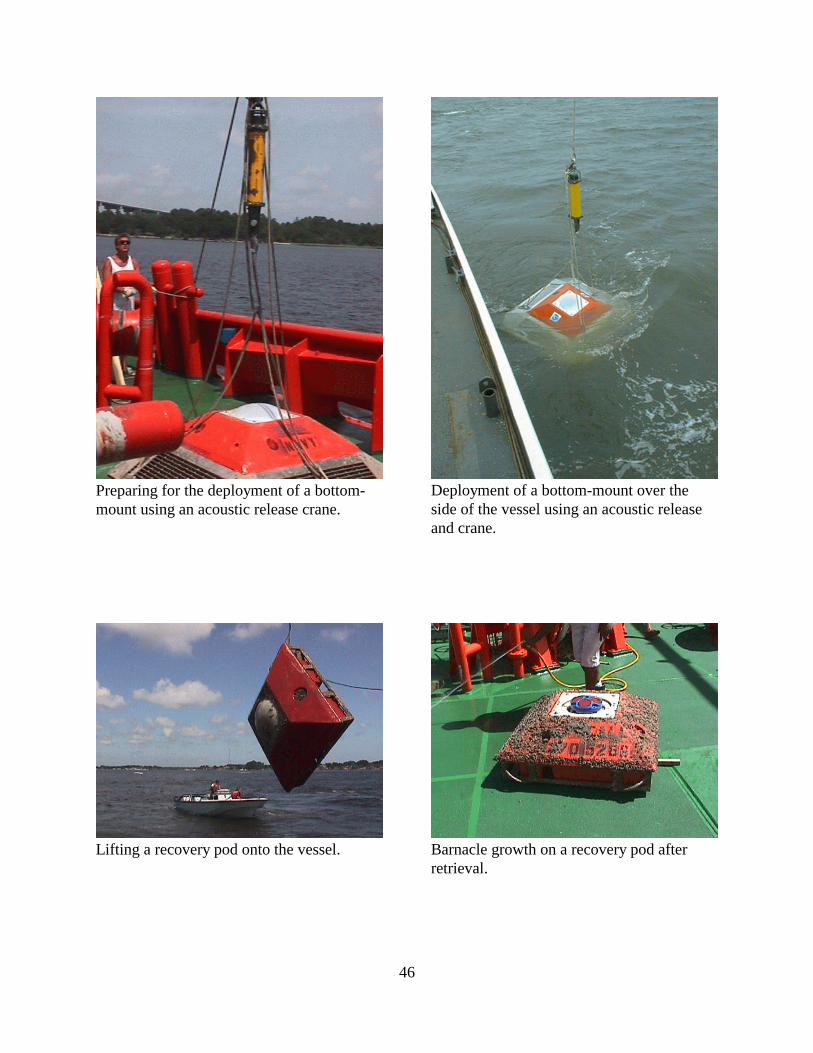
46
Deployment of a bottom-mount over theside of the vessel using an acoustic releaseand crane.
Preparing for the deployment of a bottom-mount using an acoustic release crane.
Lifting a recovery pod onto the vessel. Barnacle growth on a recovery pod afterretrieval.

47
APPENDIX B. Tidal Current Tables, 2000 (Tables 1 and 2 for the St. Johns River)

48

Slack Maximum Slack Maximum Slack Maximum Slack Maximum Slack Maximum Slack Maximumh m h m knots h m h m knots h m h m knots h m h m knots h m h m knots h m h m knots
St. Johns River Entrance, Florida, 2000F–Flood, Dir. 262 ° True E–Ebb, Dir. 081 ° True
January
1 0016 0310 2.0�
Sa 0631 1011 2.0 �1307 1553 1.4
�1835 2158 2.0 �
2 0104 0406 2.0�
Su 0720 1056 2.0 �1359 1651 1.5
�1925 2238 1.9 �
3 0152 0452 2.1�
M 0805 1139 2.0 �1447 1732 1.5
�2011 2314 1.9 �
4 0237 0531 2.2�
Tu 0848 1219 2.0 �1533 1805 1.6
�2054 2345 1.9 �
5 0320 0607 2.3�
W 0929 1253 2.0 �1615 1838 1.6
�2136
6 0017 1.9 �Th 0359 0645 2.3
�1009 1315 2.0 �1657 1913 1.6
�2216
7 0051 1.9 �F 0438 0723 2.3
�1048 1336 2.1 �1737 1952 1.6
�2255
8 0128 1.9 �Sa 0516 0804 2.3
�1128 1408 2.1 �1818 2033 1.6
�2335
9 0208 1.9 �Su 0556 0848 2.3
�1208 1444 2.1 �1859 2118 1.6
�
10 0016 0250 1.9 �M 0641 0934 2.2
�1247 1524 2.1 �1939 2204 1.8
�
11 0101 0334 1.9 �Tu 0730 1021 2.1
�1327 1606 2.1 �2019 2251 1.9
�
12 0148 0422 2.0 �W 0823 1109 2.0
�1408 1651 2.1 �2100 2338 2.1
�
13 0238 0513 2.0 �Th 0919 1158 2.0
�1451 1741 2.1 �2142
14 0026 2.3�
F 0332 0609 2.0 �1015 1247 1.9
�1540 1834 2.2 �2228
15 0116 2.4�
Sa 0430 0707 2.1 �1113 1340 1.8
�1636 1930 2.2 �2318
16 0210 2.5�
Su 0531 0807 2.2 �1213 1437 1.7
�1737 2027 2.2 �
17 0013 0308 2.6�
M 0632 0906 2.3 �1315 1539 1.7
�1840 2124 2.3 �
18 0111 0409 2.7�
Tu 0731 1005 2.3 �1417 1642 1.8
�1940 2221 2.4 �
19 0211 0509 2.9�
W 0828 1104 2.4 �1516 1741 1.9
�2037 2318 2.4 �
20 0309 0605 3.0�
Th 0923 1204 2.5 �1611 1837 2.0
�2133
21 0016 2.4 �F 0406 0659 3.0
�1016 1303 2.5 �1703 1930 2.1
�2228
22 0114 2.4 �Sa 0501 0752 2.9
�1109 1400 2.4 �1754 2023 2.1
�2325
23 0212 2.3 �Su 0558 0846 2.7
�1201 1452 2.4 �1845 2117 2.1
�
24 0021 0311 2.2 �M 0656 0941 2.5
�1251 1542 2.2 �1935 2211 2.1
�
25 0118 0414 2.0 �Tu 0756 1035 2.2
�1341 1633 2.1 �2025 2303 2.1
�
26 0213 0536 1.9 �W 0855 1127 2.0
�1430 1728 2.0 �2114 2351 2.1
�
27 0308 0653 1.8 �Th 0951 1216 1.7
�1520 1831 1.9 �2201
28 0037 2.0�
F 0403 0753 1.8 �1045 1303 1.6
�1610 1933 1.8 �2249
29 0124 2.0�
Sa 0457 0845 1.7 �1136 1352 1.4
�1702 2026 1.8 �2337
30 0213 1.9�
Su 0551 0933 1.7 �1228 1445 1.3
�1756 2112 1.8 �
31 0027 0306 1.8�
M 0643 1018 1.7 �1321 1545 1.3
�1848 2155 1.8 �
February
1 0117 0402 1.9�
Tu 0732 1103 1.8 �1412 1642 1.3
�1938 2235 1.8 �
2 0206 0453 2.0�
W 0818 1146 1.8 �1501 1728 1.4
�2025 2313 1.8 �
3 0252 0538 2.1�
Th 0901 1224 1.9 �1547 1808 1.5
�2108 2349 1.9 �
4 0335 0619 2.2�
F 0942 1250 2.0 �1629 1846 1.6
�2149
5 0026 1.9 �Sa 0416 0659 2.3
�1022 1312 2.0 �1708 1926 1.7
�2230
6 0105 2.0 �Su 0456 0741 2.3
�1101 1342 2.1 �1746 2007 1.8
�2311
7 0145 2.0 �M 0538 0824 2.3
�1140 1418 2.2 �1823 2050 1.9
�2353
8 0227 2.1 �Tu 0623 0909 2.2
�1219 1456 2.2 �1901 2136 2.1
�
9 0037 0312 2.1 �W 0712 0957 2.1
�1259 1538 2.2 �1941 2223 2.2
�
10 0124 0358 2.2 �Th 0804 1045 2.0
�1341 1623 2.2 �2024 2311 2.4
�
11 0213 0448 2.2 �F 0859 1134 1.9
�1426 1712 2.2 �2111
12 0001 2.5�
Sa 0306 0542 2.2 �0955 1225 1.9
�1516 1806 2.1 �2202
13 0052 2.5�
Su 0404 0641 2.1 �1053 1318 1.8
�1614 1905 2.1 �2257
14 0147 2.5�
M 0508 0743 2.1 �1154 1415 1.7
�1719 2006 2.1 �2356
15 0246 2.5�
Tu 0613 0848 2.1 �1258 1519 1.6
�1825 2109 2.2 �
16 0058 0351 2.6�
W 0715 0954 2.2 �1402 1627 1.7
�1928 2211 2.2 �
17 0201 0455 2.7�
Th 0814 1100 2.3 �1501 1731 1.9
�2026 2314 2.3 �
18 0301 0555 2.8�
F 0909 1206 2.4 �1554 1827 2.0
�2122
19 0017 2.4 �Sa 0358 0649 2.8
�1000 1304 2.4 �1642 1917 2.2
�2216
20 0118 2.4 �Su 0452 0739 2.7
�1050 1352 2.4 �1728 2004 2.3
�2308
21 0213 2.4 �M 0545 0829 2.6
�1138 1433 2.3 �1813 2052 2.3
�
22 0000 0302 2.3 �Tu 0639 0918 2.3
�1225 1511 2.2 �1858 2139 2.2
�
23 0051 0349 2.1 �W 0733 1007 2.1
�1311 1551 2.1 �1944 2225 2.2
�
24 0141 0435 2.0 �Th 0826 1054 1.8
�1356 1633 2.0 �2031 2311 2.1
�
25 0230 0525 1.8 �F 0918 1139 1.7
�1442 1720 1.8 �2119 2355 2.0
�
26 0320 0633 1.7 �Sa 1007 1222 1.5
�1529 1812 1.7 �2208
27 0040 1.9�
Su 0412 0745 1.6 �1056 1307 1.4
�1620 1911 1.7 �2257
28 0127 1.8�
M 0505 0840 1.5 �1146 1356 1.3
�1714 2010 1.6 �2348
29 0218 1.7�
Tu 0600 0929 1.6 �1239 1450 1.2
�1810 2104 1.7 �
March
1 0040 0314 1.7�
W 0653 1016 1.6 �1333 1550 1.3
�1904 2152 1.7 �
2 0132 0411 1.8�
Th 0743 1059 1.7 �1425 1646 1.4
�1953 2236 1.8 �
3 0222 0504 2.0�
F 0828 1135 1.8 �1511 1734 1.6
�2039 2318 1.9 �
4 0309 0550 2.1�
Sa 0911 1204 2.0 �1553 1816 1.8
�2122 2359 2.0 �
5 0354 0633 2.2�
Su 0951 1234 2.1 �1631 1857 2.0
�2204
6 0040 2.1 �M 0437 0716 2.2
�1030 1309 2.2 �1707 1939 2.2
�2245
7 0122 2.2 �Tu 0521 0759 2.2
�1109 1347 2.2 �1744 2022 2.3
�2328
8 0205 2.3 �W 0606 0845 2.1
�1150 1428 2.3 �1822 2108 2.4
�
9 0013 0249 2.4 �Th 0655 0933 2.1
�1232 1511 2.3 �1905 2157 2.5
�
10 0101 0335 2.4 �F 0747 1023 2.0
�1318 1558 2.2 �1953 2247 2.5
�
11 0151 0425 2.3 �Sa 0842 1114 1.9
�1407 1648 2.2 �2046 2338 2.5
�
12 0246 0519 2.2 �Su 0940 1206 1.8
�1501 1743 2.1 �2143
13 0031 2.5�
M 0345 0620 2.1 �1040 1300 1.7
�1602 1846 2.0 �2243
14 0128 2.4�
Tu 0450 0728 2.0 �1142 1400 1.6
�1709 1955 1.9 �2345
15 0229 2.4�
W 0557 0844 2.0 �1245 1506 1.6
�1817 2108 2.0 �
16 0049 0337 2.4�
Th 0700 1002 2.1 �1346 1619 1.7
�1920 2222 2.1 �
17 0153 0446 2.5�
F 0758 1110 2.2 �1442 1725 2.0
�2018 2331 2.3 �
18 0253 0547 2.6�
Sa 0851 1206 2.3 �1532 1817 2.2
�2111
19 0032 2.4 �Su 0349 0639 2.6
�0941 1253 2.4 �1616 1901 2.4
�2201
20 0124 2.5 �M 0441 0726 2.5
�1027 1332 2.3 �1658 1942 2.5
�2249
21 0209 2.4 �Tu 0531 0810 2.3
�1112 1405 2.3 �1739 2023 2.4
�2336
22 0246 2.4 �W 0619 0853 2.1
�1155 1437 2.2 �1820 2104 2.4
�
23 0022 0317 2.2 �Th 0707 0936 1.9
�1239 1513 2.1 �1903 2147 2.3
�
24 0107 0348 2.0 �F 0755 1019 1.7
�1322 1552 1.9 �1949 2232 2.1
�
25 0152 0426 1.9 �Sa 0842 1102 1.6
�1405 1636 1.8 �2037 2316 2.0
�
26 0239 0509 1.7 �Su 0930 1145 1.5
�1450 1723 1.7 �2127
27 0001 1.9�
M 0327 0600 1.6 �1018 1229 1.4
�1539 1816 1.6 �2217
28 0048 1.8�
Tu 0419 0659 1.5 �1107 1317 1.3
�1633 1914 1.6 �2308
29 0138 1.8�
W 0514 0806 1.5 �1159 1409 1.3
�1730 2013 1.6 �
30 0001 0232 1.7�
Th 0609 0905 1.6 �1251 1505 1.3
�1827 2108 1.6 �
31 0055 0329 1.7�
F 0701 0952 1.7 �1341 1603 1.5
�1920 2158 1.8 �
Time meridian 75° W. 0000 is midnight. 1200 is noon.

Slack Maximum Slack Maximum Slack Maximum Slack Maximum Slack Maximum Slack Maximumh m h m knots h m h m knots h m h m knots h m h m knots h m h m knots h m h m knots
St. Johns River Entrance, Florida, 2000F–Flood, Dir. 262 ° True E–Ebb, Dir. 081 ° True
April
1 0149 0426 1.8�
Sa 0749 1033 1.9 �1428 1655 1.8
�2008 2244 1.9 �
2 0241 0517 2.0�
Su 0833 1113 2.0 �1509 1742 2.0
�2053 2329 2.1 �
3 0330 0604 2.1�
M 0915 1153 2.1 �1548 1826 2.3
�2136
4 0012 2.3 �Tu 0416 0649 2.1
�0956 1233 2.2 �1626 1909 2.5
�2219
5 0056 2.4 �W 0501 0733 2.1
�1037 1316 2.3 �1705 1954 2.6
�2303
6 0141 2.5 �Th 0548 0820 2.1
�1120 1400 2.3 �1748 2041 2.7
�2350
7 0227 2.5 �F 0637 0909 2.0
�1207 1446 2.3 �1835 2132 2.7
�
8 0040 0314 2.5 �Sa 0731 1002 1.9
�1258 1535 2.2 �1929 2225 2.6
�
9 0133 0406 2.3 �Su 0829 1056 1.8
�1352 1627 2.1 �2028 2319 2.5
�
10 0230 0502 2.2 �M 0930 1151 1.8
�1451 1726 1.9 �2130
11 0015 2.5�
Tu 0331 0606 2.1 �1030 1248 1.7
�1555 1835 1.8 �2233
12 0113 2.4�
W 0435 0729 2.0 �1130 1349 1.7
�1703 2009 1.8 �2337
13 0216 2.2�
Th 0540 0905 2.1 �1229 1458 1.7
�1810 2136 1.9 �
14 0041 0326 2.2�
F 0642 1009 2.1 �1326 1614 1.9
�1911 2240 2.1 �
15 0145 0439 2.2�
Sa 0739 1102 2.2 �1417 1716 2.1
�2006 2338 2.3 �
16 0244 0540 2.3�
Su 0830 1150 2.3 �1504 1803 2.4
�2056
17 0030 2.4 �M 0338 0629 2.3
�0917 1231 2.3 �1547 1841 2.5
�2143
18 0116 2.5 �Tu 0428 0710 2.2
�1002 1305 2.2 �1627 1917 2.6
�2227
19 0154 2.4 �W 0513 0748 2.1
�1044 1334 2.2 �1706 1953 2.5
�2310
20 0223 2.3 �Th 0557 0825 1.9
�1126 1404 2.1 �1745 2031 2.4
�2353
21 0245 2.2 �F 0640 0904 1.8
�1207 1439 2.0 �1827 2113 2.3
�
22 0035 0313 2.1 �Sa 0724 0945 1.6
�1248 1518 1.9 �1911 2156 2.1
�
23 0118 0349 1.9 �Su 0809 1028 1.5
�1331 1600 1.8 �1957 2242 2.0
�
24 0202 0431 1.8 �M 0856 1112 1.5
�1415 1645 1.7 �2046 2328 2.0
�
25 0247 0519 1.7 �Tu 0944 1157 1.4
�1502 1735 1.6 �2137
26 0014 1.9�
W 0336 0613 1.7 �1032 1244 1.4
�1554 1830 1.6 �2228
27 0103 1.8�
Th 0427 0710 1.7 �1119 1334 1.5
�1651 1928 1.6 �2322
28 0154 1.8�
F 0521 0807 1.7 �1207 1427 1.6
�1749 2026 1.7 �
29 0018 0249 1.7�
Sa 0614 0857 1.8 �1253 1522 1.8
�1844 2119 1.8 �
30 0116 0346 1.7�
Su 0704 0944 2.0 �1338 1616 2.0
�1935 2209 2.0 �
May
1 0211 0442 1.8�
M 0751 1029 2.1 �1422 1707 2.3
�2022 2256 2.2 �
2 0303 0533 1.9�
Tu 0836 1114 2.2 �1505 1754 2.6
�2108 2343 2.4 �
3 0352 0621 2.0�
W 0920 1159 2.3 �1548 1841 2.8
�2153
4 0030 2.5 �Th 0439 0708 2.1
�1005 1246 2.4 �1632 1928 2.9
�2240
5 0117 2.6 �F 0528 0756 2.0
�1053 1334 2.4 �1720 2017 2.9
�2330
6 0206 2.6 �Sa 0620 0848 2.0
�1145 1423 2.3 �1812 2110 2.8
�
7 0022 0256 2.5 �Su 0716 0943 1.9
�1241 1515 2.2 �1910 2206 2.7
�
8 0118 0350 2.3 �M 0817 1040 1.8
�1340 1611 2.0 �2013 2303 2.5
�
9 0216 0450 2.2 �Tu 0918 1139 1.8
�1442 1715 1.8 �2118
10 0000 2.4�
W 0316 0604 2.1 �1017 1238 1.8
�1548 1852 1.7 �2223
11 0059 2.3�
Th 0418 0756 2.1 �1113 1339 1.8
�1655 2036 1.9 �2327
12 0202 2.1�
F 0520 0901 2.1 �1207 1447 1.9
�1758 2139 2.0 �
13 0030 0313 2.0�
Sa 0619 0953 2.2 �1258 1559 2.0
�1857 2234 2.2 �
14 0132 0427 2.0�
Su 0714 1040 2.2 �1347 1657 2.2
�1950 2327 2.3 �
15 0230 0527 2.0�
M 0805 1124 2.2 �1434 1741 2.4
�2038
16 0015 2.4 �Tu 0322 0614 2.0
�0851 1202 2.2 �1517 1817 2.5
�2122
17 0058 2.4 �W 0409 0651 2.0
�0934 1235 2.1 �1557 1851 2.5
�2204
18 0135 2.3 �Th 0452 0724 1.9
�1016 1303 2.1 �1637 1925 2.5
�2245
19 0200 2.2 �F 0533 0757 1.8
�1056 1334 2.0 �1716 2002 2.4
�2325
20 0217 2.1 �Sa 0614 0833 1.7
�1137 1409 2.0 �1755 2042 2.3
�
21 0006 0245 2.0 �Su 0656 0914 1.5
�1217 1447 1.9 �1837 2125 2.2
�
22 0048 0321 2.0 �M 0741 0957 1.5
�1259 1528 1.8 �1922 2211 2.1
�
23 0130 0403 1.9 �Tu 0827 1043 1.5
�1343 1613 1.7 �2010 2257 2.0
�
24 0213 0448 1.9 �W 0913 1129 1.5
�1429 1701 1.7 �2101 2344 2.0
�
25 0258 0537 1.8 �Th 0957 1215 1.6
�1519 1753 1.6 �2153
26 0032 1.9�
F 0344 0629 1.8 �1040 1302 1.7
�1613 1850 1.7 �2248
27 0121 1.8�
Sa 0433 0722 1.9 �1122 1352 1.9
�1710 1947 1.8 �2344
28 0213 1.7�
Su 0524 0813 2.0 �1205 1444 2.1
�1807 2042 1.9 �
29 0041 0309 1.7�
M 0617 0902 2.1 �1251 1539 2.3
�1900 2134 2.1 �
30 0139 0406 1.7�
Tu 0708 0951 2.2 �1338 1633 2.6
�1951 2224 2.3 �
31 0234 0501 1.8�
W 0758 1039 2.3 �1427 1725 2.8
�2041 2314 2.5 �
June
1 0326 0553 1.9�
Th 0848 1129 2.4 �1517 1815 3.0
�2130
2 0004 2.6 �F 0417 0643 2.0
�0938 1219 2.5 �1607 1905 3.0
�2220
3 0055 2.6 �Sa 0509 0734 2.0
�1030 1311 2.4 �1659 1957 3.0
�2313
4 0148 2.5 �Su 0603 0828 1.9
�1126 1404 2.3 �1755 2051 2.8
�
5 0007 0242 2.5 �M 0701 0925 1.9
�1225 1459 2.1 �1855 2148 2.7
�
6 0103 0339 2.3 �Tu 0801 1025 1.8
�1327 1559 2.0 �2000 2247 2.5
�
7 0201 0443 2.2 �W 0900 1126 1.9
�1431 1712 1.8 �2106 2346 2.3
�
8 0258 0616 2.1 �Th 0956 1224 1.9
�1535 1917 1.8 �2210
9 0044 2.2�
F 0357 0741 2.1 �1048 1323 2.0
�1638 2027 1.9 �2312
10 0145 2.0�
Sa 0455 0838 2.1 �1138 1423 2.0
�1739 2124 2.1 �
11 0013 0252 1.8�
Su 0551 0927 2.1 �1227 1527 2.1
�1835 2216 2.2 �
12 0112 0405 1.7�
M 0645 1012 2.1 �1315 1627 2.2
�1927 2305 2.2 �
13 0208 0506 1.7�
Tu 0736 1054 2.1 �1403 1714 2.3
�2014 2352 2.2 �
14 0259 0552 1.7�
W 0822 1133 2.1 �1448 1751 2.4
�2058
15 0035 2.2 �Th 0345 0628 1.7
�0906 1207 2.0 �1531 1825 2.4
�2140
16 0113 2.2 �F 0427 0658 1.7
�0948 1236 2.0 �1611 1859 2.4
�2220
17 0141 2.1 �Sa 0508 0729 1.6
�1028 1307 2.0 �1650 1936 2.3
�2300
18 0157 2.1 �Su 0549 0805 1.6
�1109 1342 1.9 �1729 2015 2.3
�2341
19 0223 2.0 �M 0631 0846 1.5
�1149 1420 1.8 �1809 2058 2.2
�
20 0021 0258 2.0 �Tu 0714 0929 1.5
�1231 1501 1.8 �1852 2143 2.1
�
21 0102 0337 2.0 �W 0757 1015 1.6
�1314 1544 1.8 �1939 2229 2.1
�
22 0143 0419 2.0 �Th 0839 1100 1.7
�1400 1631 1.8 �2030 2316 2.0
�
23 0223 0504 2.0 �F 0920 1146 1.8
�1447 1721 1.8 �2123
24 0003 1.9�
Sa 0305 0552 2.0 �0959 1232 2.0
�1538 1815 1.8 �2217
25 0051 1.9�
Su 0349 0642 2.0 �1040 1320 2.2
�1633 1911 1.9 �2312
26 0141 1.8�
M 0439 0734 2.1 �1123 1411 2.3
�1730 2007 2.1 �
27 0009 0235 1.7�
Tu 0534 0827 2.2 �1211 1505 2.5
�1828 2102 2.2 �
28 0107 0333 1.7�
W 0631 0919 2.3 �1303 1602 2.7
�1923 2156 2.3 �
29 0205 0431 1.8�
Th 0727 1011 2.4 �1358 1659 2.8
�2017 2249 2.4 �
30 0302 0528 1.9�
F 0822 1104 2.5 �1454 1753 3.0
�2110 2343 2.5 �
Time meridian 75° W. 0000 is midnight. 1200 is noon.

Slack Maximum Slack Maximum Slack Maximum Slack Maximum Slack Maximum Slack Maximumh m h m knots h m h m knots h m h m knots h m h m knots h m h m knots h m h m knots
St. Johns River Entrance, Florida, 2000F–Flood, Dir. 262 ° True E–Ebb, Dir. 081 ° True
July
1 0357 0622 2.0�
Sa 0916 1158 2.5 �1549 1846 3.0
�2203
2 0038 2.5 �Su 0451 0716 2.0
�1012 1253 2.4 �1644 1939 3.0
�2257
3 0134 2.5 �M 0546 0811 2.0
�1110 1349 2.3 �1742 2034 2.8
�2351
4 0231 2.4 �Tu 0642 0908 2.0
�1211 1448 2.2 �1842 2132 2.7
�
5 0046 0329 2.3 �W 0738 1008 2.0
�1312 1551 2.0 �1946 2230 2.4
�
6 0141 0431 2.2 �Th 0833 1106 2.0
�1413 1718 1.9 �2050 2328 2.2
�
7 0235 0550 2.1 �F 0926 1202 2.1
�1513 1859 1.9 �2153
8 0024 2.0�
Sa 0330 0707 2.1 �1016 1255 2.1
�1613 2004 2.0 �2252
9 0120 1.8�
Su 0424 0804 2.0 �1105 1347 2.1
�1711 2059 2.0 �2349
10 0219 1.6�
M 0519 0854 2.0 �1153 1443 2.1
�1806 2150 2.0 �
11 0045 0326 1.5�
Tu 0613 0940 2.0 �1242 1542 2.1
�1858 2237 2.0 �
12 0139 0433 1.5�
W 0704 1023 2.0 �1332 1638 2.1
�1947 2324 2.0 �
13 0230 0523 1.5�
Th 0753 1104 1.9 �1420 1722 2.1
�2032
14 0008 2.0 �F 0317 0600 1.5
�0838 1140 1.9 �1505 1759 2.2
�2115
15 0048 2.0 �Sa 0401 0631 1.6
�0921 1212 1.9 �1547 1834 2.3
�2156
16 0121 2.0 �Su 0442 0703 1.6
�1002 1243 1.9 �1627 1911 2.3
�2236
17 0141 2.0 �M 0523 0739 1.6
�1043 1318 1.9 �1706 1950 2.3
�2315
18 0202 2.0 �Tu 0603 0819 1.6
�1123 1356 1.9 �1746 2032 2.2
�2355
19 0233 2.1 �W 0643 0901 1.7
�1205 1436 1.9 �1829 2116 2.1
�
20 0034 0310 2.1 �Th 0722 0945 1.7
�1247 1518 1.9 �1915 2203 2.1
�
21 0112 0349 2.1 �F 0801 1031 1.9
�1331 1604 1.9 �2006 2249 2.0
�
22 0151 0432 2.1 �Sa 0839 1117 2.1
�1417 1652 2.0 �2058 2336 1.9
�
23 0231 0518 2.1 �Su 0920 1203 2.3
�1506 1744 2.0 �2151
24 0024 1.9�
M 0314 0608 2.1 �1003 1251 2.4
�1600 1839 2.1 �2245
25 0113 1.8�
Tu 0404 0701 2.1 �1050 1342 2.5
�1659 1936 2.1 �2341
26 0207 1.7�
W 0501 0757 2.2 �1142 1437 2.6
�1800 2034 2.2 �
27 0040 0305 1.7�
Th 0603 0853 2.3 �1239 1537 2.6
�1900 2132 2.3 �
28 0142 0407 1.7�
F 0705 0949 2.4 �1339 1637 2.8
�1958 2229 2.3 �
29 0242 0508 1.8�
Sa 0804 1046 2.4 �1438 1736 2.9
�2053 2328 2.4 �
30 0339 0606 2.0�
Su 0902 1143 2.4 �1537 1831 3.0
�2147
31 0026 2.5 �M 0433 0700 2.1
�0959 1241 2.4 �1634 1925 2.9
�2240
August
1 0124 2.5 �Tu 0525 0754 2.1
�1056 1341 2.4 �1731 2018 2.8
�2333
2 0219 2.4 �W 0616 0848 2.2
�1154 1440 2.3 �1829 2114 2.6
�
3 0025 0312 2.4 �Th 0707 0944 2.2
�1251 1542 2.1 �1930 2210 2.3
�
4 0117 0404 2.2 �F 0759 1038 2.2
�1348 1657 2.0 �2031 2305 2.1
�
5 0208 0500 2.1 �Sa 0850 1130 2.2
�1444 1824 1.9 �2129 2357 1.9
�
6 0259 0607 2.0 �Su 0940 1218 2.1
�1539 1931 1.9 �2225
7 0047 1.7�
M 0350 0717 1.9 �1029 1306 2.1
�1635 2027 1.8 �2318
8 0137 1.5�
Tu 0443 0815 1.8 �1119 1356 2.0
�1730 2117 1.8 �
9 0010 0231 1.4�
W 0538 0905 1.8 �1209 1451 1.9
�1824 2205 1.8 �
10 0103 0334 1.3�
Th 0631 0951 1.8 �1301 1550 1.9
�1915 2251 1.8 �
11 0155 0438 1.3�
F 0722 1034 1.8 �1351 1644 1.9
�2002 2336 1.8 �
12 0244 0524 1.4�
Sa 0810 1113 1.8 �1438 1728 2.0
�2046
13 0018 1.9 �Su 0330 0600 1.5
�0855 1147 1.9 �1522 1808 2.1
�2128
14 0052 2.0 �M 0413 0635 1.6
�0937 1219 1.9 �1604 1846 2.2
�2208
15 0112 2.0 �Tu 0452 0712 1.7
�1018 1254 1.9 �1644 1925 2.2
�2247
16 0133 2.1 �W 0529 0750 1.8
�1057 1332 2.0 �1725 2007 2.2
�2325
17 0204 2.1 �Th 0605 0832 1.9
�1137 1411 2.0 �1808 2050 2.1
�
18 0003 0240 2.1 �F 0641 0915 2.0
�1219 1453 2.1 �1855 2136 2.0
�
19 0041 0319 2.1 �Sa 0719 1001 2.2
�1302 1537 2.2 �1944 2223 2.0
�
20 0120 0401 2.1 �Su 0800 1048 2.3
�1348 1624 2.2 �2035 2311 1.9
�
21 0202 0447 2.1 �M 0844 1136 2.4
�1438 1715 2.2 �2128 2359 1.8
�
22 0247 0538 2.1 �Tu 0933 1225 2.5
�1533 1810 2.1 �2223
23 0050 1.8�
W 0339 0633 2.1 �1025 1318 2.5
�1633 1910 2.1 �2321
24 0144 1.7�
Th 0440 0733 2.1 �1123 1414 2.5
�1737 2012 2.1 �
25 0022 0244 1.6�
F 0547 0834 2.2 �1224 1516 2.5
�1841 2116 2.2 �
26 0125 0349 1.7�
Sa 0653 0936 2.2 �1327 1620 2.6
�1941 2218 2.3 �
27 0225 0454 1.8�
Su 0754 1037 2.3 �1429 1722 2.7
�2038 2320 2.4 �
28 0321 0553 2.1�
M 0852 1139 2.4 �1528 1819 2.8
�2131
29 0019 2.4 �Tu 0411 0646 2.3
�0947 1240 2.5 �1625 1911 2.8
�2221
30 0113 2.5 �W 0459 0736 2.4
�1041 1339 2.5 �1720 2002 2.6
�2311
31 0201 2.4 �Th 0545 0825 2.4
�1134 1434 2.4 �1815 2054 2.4
�
September
1 0000 0245 2.3 �F 0632 0914 2.4
�1227 1525 2.3 �1910 2145 2.1
�
2 0048 0329 2.2 �Sa 0720 1003 2.3
�1319 1617 2.1 �2006 2236 1.9
�
3 0136 0414 2.0 �Su 0810 1052 2.2
�1410 1717 1.9 �2100 2324 1.7
�
4 0225 0503 1.9 �M 0901 1139 2.1
�1502 1838 1.7 �2152
5 0010 1.5�
Tu 0314 0600 1.7 �0952 1226 2.0
�1555 1944 1.6 �2243
6 0056 1.4�
W 0406 0710 1.7 �1043 1314 1.8
�1649 2038 1.6 �2333
7 0144 1.3�
Th 0500 0819 1.6 �1135 1405 1.7
�1744 2127 1.6 �
8 0024 0238 1.2�
F 0556 0913 1.7 �1227 1500 1.7
�1838 2212 1.7 �
9 0117 0339 1.3�
Sa 0651 0959 1.7 �1318 1558 1.8
�1927 2256 1.8 �
10 0207 0436 1.4�
Su 0741 1040 1.8 �1409 1651 1.9
�2013 2334 1.9 �
11 0254 0523 1.6�
M 0827 1116 1.8 �1456 1737 2.0
�2055
12 0003 2.0 �Tu 0336 0603 1.8
�0910 1152 1.9 �1540 1818 2.1
�2136
13 0026 2.1 �W 0414 0641 2.0
�0950 1228 2.0 �1623 1859 2.2
�2214
14 0055 2.1 �Th 0449 0720 2.2
�1030 1306 2.2 �1705 1940 2.1
�2252
15 0130 2.2 �F 0524 0801 2.3
�1109 1346 2.3 �1749 2024 2.1
�2330
16 0208 2.2 �Sa 0600 0845 2.4
�1151 1428 2.3 �1834 2109 2.0
�
17 0010 0248 2.2 �Su 0639 0931 2.4
�1236 1512 2.3 �1923 2158 1.9
�
18 0052 0332 2.2 �M 0724 1020 2.5
�1324 1559 2.3 �2015 2248 1.8
�
19 0138 0420 2.1 �Tu 0815 1111 2.5
�1415 1650 2.2 �2111 2339 1.8
�
20 0228 0513 2.0 �W 0910 1203 2.5
�1512 1747 2.1 �2209
21 0031 1.7�
Th 0326 0611 2.0 �1009 1258 2.4
�1614 1850 2.1 �2308
22 0127 1.7�
F 0431 0716 1.9 �1111 1356 2.4
�1720 2000 2.1 �
23 0009 0229 1.6�
Sa 0540 0826 2.0 �1215 1500 2.4
�1825 2111 2.1 �
24 0110 0337 1.7�
Su 0646 0937 2.1 �1319 1607 2.4
�1925 2218 2.2 �
25 0207 0444 2.0�
M 0747 1046 2.3 �1422 1712 2.5
�2020 2318 2.3 �
26 0259 0542 2.2�
Tu 0842 1150 2.4 �1521 1808 2.6
�2112
27 0010 2.4 �W 0346 0631 2.5
�0934 1248 2.5 �1616 1859 2.6
�2200
28 0056 2.4 �Th 0430 0716 2.6
�1024 1339 2.5 �1707 1945 2.4
�2247
29 0136 2.3 �F 0513 0759 2.6
�1112 1422 2.5 �1758 2031 2.2
�2333
30 0215 2.2 �Sa 0556 0843 2.5
�1200 1500 2.3 �1848 2117 2.0
�
Time meridian 75° W. 0000 is midnight. 1200 is noon.
Slack Maximum Slack Maximum Slack Maximum Slack Maximum Slack Maximum Slack Maximumh m h m knots h m h m knots h m h m knots h m h m knots h m h m knots h m h m knots
St. Johns River Entrance, Florida, 2000F–Flood, Dir. 262 ° True E–Ebb, Dir. 081 ° True
October
1 0018 0254 2.1 �Su 0641 0928 2.4
�1248 1536 2.1 �1938 2203 1.7
�
2 0103 0335 2.0 �M 0730 1015 2.2
�1335 1614 1.9 �2028 2248 1.6
�
3 0149 0419 1.8 �Tu 0821 1101 2.1
�1424 1659 1.7 �2117 2333 1.5
�
4 0237 0508 1.7 �W 0913 1148 1.9
�1514 1753 1.6 �2206
5 0018 1.4�
Th 0328 0604 1.6 �1005 1235 1.8
�1606 1927 1.5 �2256
6 0105 1.3�
F 0422 0708 1.5 �1057 1324 1.7
�1700 2034 1.6 �2345
7 0156 1.3�
Sa 0520 0816 1.5 �1149 1417 1.7
�1754 2120 1.6 �
8 0036 0251 1.4�
Su 0616 0912 1.6 �1243 1513 1.7
�1846 2158 1.8 �
9 0125 0348 1.5�
M 0709 0958 1.7 �1336 1609 1.7
�1933 2231 1.9 �
10 0210 0440 1.7�
Tu 0756 1039 1.9 �1427 1701 1.9
�2017 2304 2.0 �
11 0252 0525 2.0�
W 0839 1118 2.0 �1515 1747 2.0
�2058 2338 2.1 �
12 0330 0608 2.3�
Th 0920 1157 2.2 �1600 1830 2.0
�2138
13 0015 2.2 �F 0407 0649 2.5
�1001 1238 2.3 �1643 1913 2.1
�2217
14 0055 2.2 �Sa 0444 0731 2.6
�1042 1319 2.4 �1727 1957 2.0
�2257
15 0136 2.3 �Su 0523 0817 2.6
�1126 1403 2.5 �1813 2044 1.9
�2340
16 0220 2.2 �M 0606 0905 2.6
�1213 1449 2.4 �1903 2134 1.8
�
17 0027 0307 2.2 �Tu 0656 0956 2.6
�1303 1537 2.4 �1959 2227 1.8
�
18 0119 0357 2.1 �W 0753 1050 2.5
�1358 1630 2.2 �2058 2321 1.7
�
19 0216 0452 1.9 �Th 0855 1145 2.5
�1457 1730 2.1 �2159
20 0017 1.7�
F 0319 0555 1.8 �0959 1242 2.4
�1559 1839 2.0 �2258
21 0116 1.7�
Sa 0427 0711 1.8 �1103 1342 2.3
�1704 2002 2.0 �2356
22 0218 1.8�
Su 0535 0845 1.9 �1208 1447 2.2
�1807 2121 2.1 �
23 0051 0327 1.9�
M 0639 1001 2.1 �1312 1557 2.2
�1906 2220 2.2 �
24 0144 0434 2.1�
Tu 0737 1102 2.3 �1414 1704 2.3
�2000 2310 2.3 �
25 0234 0529 2.4�
W 0830 1157 2.4 �1511 1759 2.3
�2050 2355 2.3 �
26 0319 0614 2.6�
Th 0918 1247 2.5 �1604 1846 2.3
�2137
27 0035 2.3 �F 0402 0654 2.7
�1004 1331 2.5 �1652 1927 2.2
�2221
28 0110 2.2 �Sa 0443 0733 2.7
�1049 1406 2.4 �1738 2007 2.0
�2304
29 0145 2.2 �Su 0525 0813 2.5
�1134 1434 2.3 �1823 2047 1.8
�2347
30 0222 2.1 �M 0608 0855 2.4
�1218 1502 2.1 �1908 2129 1.6
�
31 0031 0301 1.9 �Tu 0653 0940 2.2
�1303 1537 1.9 �1955 2213 1.5
�
November
1 0116 0343 1.8 �W 0742 1026 2.0
�1348 1618 1.8 �2043 2258 1.4
�
2 0202 0429 1.7 �Th 0833 1113 1.9
�1435 1706 1.7 �2132 2344 1.4
�
3 0251 0520 1.6 �F 0925 1200 1.8
�1523 1801 1.6 �2219
4 0031 1.4�
Sa 0345 0616 1.5 �1018 1248 1.8
�1613 1901 1.6 �2306
5 0119 1.5�
Su 0441 0718 1.5 �1111 1338 1.7
�1706 2000 1.7 �2352
6 0210 1.6�
M 0538 0818 1.6 �1205 1431 1.6
�1758 2049 1.8 �
7 0037 0304 1.7�
Tu 0631 0910 1.7 �1300 1527 1.6
�1848 2132 1.9 �
8 0121 0357 2.0�
W 0720 0957 1.9 �1355 1622 1.7
�1934 2214 2.0 �
9 0204 0447 2.2�
Th 0806 1041 2.1 �1446 1712 1.8
�2018 2256 2.2 �
10 0246 0534 2.5�
F 0850 1124 2.3 �1533 1800 1.9
�2100 2338 2.3 �
11 0327 0619 2.7�
Sa 0933 1208 2.4 �1619 1845 2.0
�2142
12 0022 2.3 �Su 0409 0704 2.8
�1017 1253 2.5 �1705 1931 2.0
�2227
13 0108 2.3 �M 0453 0752 2.8
�1104 1340 2.5 �1753 2020 1.9
�2315
14 0156 2.3 �Tu 0542 0842 2.8
�1154 1429 2.5 �1846 2113 1.8
�
15 0008 0246 2.2 �W 0636 0936 2.7
�1247 1520 2.4 �1945 2209 1.8
�
16 0105 0339 2.0 �Th 0738 1032 2.5
�1344 1616 2.2 �2046 2307 1.8
�
17 0207 0437 1.9 �F 0843 1130 2.4
�1442 1718 2.1 �2145
18 0005 1.8�
Sa 0313 0547 1.7 �0949 1228 2.3
�1543 1838 2.1 �2242
19 0104 1.8�
Su 0420 0746 1.8 �1054 1328 2.2
�1645 2016 2.1 �2335
20 0206 1.9�
M 0526 0905 1.9 �1158 1433 2.0
�1746 2116 2.2 �
21 0027 0313 2.1�
Tu 0627 1003 2.1 �1301 1545 2.0
�1844 2207 2.2 �
22 0118 0418 2.3�
W 0722 1057 2.3 �1402 1654 2.0
�1938 2253 2.2 �
23 0206 0511 2.5�
Th 0813 1148 2.4 �1458 1748 2.0
�2027 2336 2.2 �
24 0252 0555 2.6�
F 0900 1235 2.5 �1548 1832 2.0
�2112
25 0014 2.2 �Sa 0336 0633 2.6
�0944 1317 2.4 �1633 1909 1.9
�2156
26 0047 2.1 �Su 0418 0709 2.6
�1027 1351 2.3 �1716 1943 1.8
�2237
27 0119 2.1 �M 0458 0747 2.5
�1110 1414 2.2 �1758 2019 1.7
�2319
28 0154 2.0 �Tu 0540 0827 2.3
�1152 1437 2.1 �1841 2058 1.6
�
29 0001 0232 1.9 �W 0622 0910 2.2
�1234 1510 2.0 �1925 2141 1.5
�
30 0045 0313 1.8 �Th 0708 0955 2.1
�1317 1549 1.9 �2012 2227 1.5
�
December
1 0130 0357 1.7 �F 0756 1041 2.0
�1400 1633 1.8 �2058 2313 1.5
�
2 0218 0444 1.6 �Sa 0847 1128 1.9
�1443 1721 1.8 �2142 2359 1.6
�
3 0308 0536 1.6 �Su 0940 1214 1.8
�1528 1812 1.8 �2224
4 0045 1.7�
M 0400 0632 1.6 �1033 1302 1.7
�1616 1905 1.8 �2306
5 0133 1.8�
Tu 0455 0730 1.7 �1128 1353 1.7
�1706 1956 1.9 �2348
6 0223 2.0�
W 0549 0825 1.8 �1223 1446 1.6
�1757 2044 2.0 �
7 0032 0316 2.2�
Th 0642 0916 2.0 �1319 1542 1.6
�1848 2132 2.1 �
8 0118 0410 2.4�
F 0732 1005 2.2 �1413 1637 1.7
�1937 2218 2.2 �
9 0205 0501 2.7�
Sa 0820 1052 2.3 �1505 1729 1.8
�2024 2306 2.3 �
10 0253 0552 2.8�
Su 0907 1141 2.5 �1554 1819 1.9
�2112 2354 2.4 �
11 0342 0641 2.9�
M 0956 1230 2.5 �1643 1908 2.0
�2202
12 0044 2.4 �Tu 0432 0731 3.0
�1046 1320 2.5 �1734 1959 1.9
�2255
13 0135 2.3 �W 0525 0823 2.9
�1138 1413 2.5 �1829 2054 1.9
�2353
14 0229 2.2 �Th 0622 0918 2.7
�1233 1507 2.4 �1928 2153 1.9
�
15 0054 0325 2.1 �F 0725 1016 2.6
�1328 1604 2.3 �2027 2252 1.9
�
16 0157 0427 1.9 �Sa 0831 1114 2.4
�1425 1709 2.2 �2124 2351 2.0
�
17 0301 0552 1.8 �Su 0937 1212 2.2
�1523 1839 2.1 �2218
18 0048 2.0�
M 0405 0750 1.9 �1041 1311 2.1
�1622 2000 2.1 �2309
19 0146 2.1�
Tu 0507 0854 2.0 �1144 1415 1.9
�1721 2056 2.1 �2359
20 0248 2.2�
W 0607 0949 2.2 �1245 1527 1.8
�1819 2146 2.1 �
21 0049 0352 2.3�
Th 0702 1041 2.2 �1343 1638 1.7
�1912 2232 2.1 �
22 0139 0450 2.3�
F 0752 1131 2.3 �1438 1733 1.8
�2002 2315 2.1 �
23 0227 0536 2.4�
Sa 0839 1218 2.3 �1527 1816 1.8
�2047 2355 2.1 �
24 0313 0614 2.5�
Su 0924 1301 2.2 �1612 1850 1.7
�2131
25 0028 2.0 �M 0356 0649 2.4
�1006 1337 2.2 �1653 1920 1.7
�2212
26 0059 2.0 �Tu 0437 0724 2.4
�1047 1403 2.1 �1734 1954 1.6
�2254
27 0132 1.9 �W 0516 0802 2.3
�1127 1420 2.0 �1815 2031 1.6
�2335
28 0208 1.9 �Th 0556 0843 2.2
�1208 1448 2.0 �1857 2113 1.6
�
29 0018 0247 1.8 �F 0639 0926 2.1
�1248 1523 2.0 �1939 2157 1.6
�
30 0101 0329 1.8 �Sa 0725 1012 2.0
�1328 1603 2.0 �2021 2242 1.7
�
31 0146 0414 1.8 �Su 0814 1058 2.0
�1407 1646 2.0 �2101 2327 1.8
�
Time meridian 75° W. 0000 is midnight. 1200 is noon.
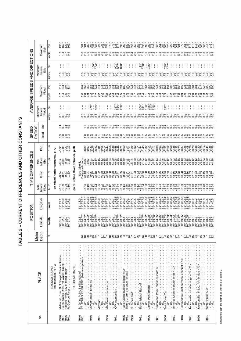
TA
BL
E 2
– C
UR
RE
NT
DIF
FE
RE
NC
ES
AN
D O
TH
ER
CO
NS
TA
NT
S
No.
PLA
CE
Met
erD
epth
PO
SIT
ION
Latit
ude
Long
itude
TIM
E D
IFF
ER
EN
CE
S
Min
.be
fore
Flo
odF
lood
Min
.be
fore
Ebb
Ebb
SP
EE
DR
AT
IOS
Flo
odE
bb
AV
ER
AG
E S
PE
ED
S A
ND
DIR
EC
TIO
NS
Min
imum
befo
reF
lood
Max
imum
Flo
od
Min
imum
befo
reE
bbM
axim
umE
bb
fth
mh
mh
mh
mkn
ots
knot
skn
ots
knot
sD
ir.D
ir.D
ir.D
ir.N
ort
hW
est
NA
SS
AU
SO
UN
DT
ime
mer
idia
n, 7
5°
W
o
n M
iam
i Har
bo
r E
ntr
ance
, p.7
2
7926
Mid
soun
d, 1
mi.
N o
f Saw
pit C
reek
ent
ranc
e .
. . .
.30
°31.
4’
81
°27.
1’
+0
01–0
24
–0 1
4–0
30
0.9
1.1
0.0
– –
1.7
312
°0.
0–
–1.
713
5°
7931
Sou
th A
mel
ia R
iver
, off
Wal
ker
Cre
ek .
. . .
. . .
. . .
.30
°32.
2’
81
°27.
9’
–1 0
9–0
21
–0 3
9–2
06
0.8
0.9
0.0
– –
1.4
341
°0.
0–
–1.
416
2°
7936
Nas
sau
Riv
er, S
W o
f Mes
a M
arsh
. . .
. . .
. . .
. . .
.30
°32.
0’
81
°28.
8’
+0
08–0
21
0 00
–0 2
20.
81.
10.
0–
–1.
529
4°
0.0
– –
1.7
129
°79
41F
t. G
eorg
e R
iver
. . .
. . .
. . .
. . .
. . .
. . .
. . .
. . .
. . .
30°2
7.4
’ 8
1°2
7.1
’–1
36
–1 2
0–1
25
–2 2
90.
20.
60.
0–
–0.
333
4°
0.0
– –
0.9
162
°
ST
. JO
HN
S R
IVE
Ro
n S
t. J
oh
ns
Riv
er E
ntr
ance
, p.6
8
7946
St.
John
s P
oint
, 5 m
iles
east
of
. . .
. . .
. . .
. . .
. . .
30°2
3.5
’ 8
1°1
8.0
’S
ee ta
ble
5.79
51S
T. J
OH
NS
RIV
ER
EN
T. (
betw
een
jetti
es)
. . .
. . .
.16
30°2
4.02
’ 8
1°2
3.15
’D
aily
pre
dict
ions
0.0
– –
2.0
262
°0.
0–
–2.
008
1°
. . .
do.
. . .
. . .
. . .
. . .
. . .
. . .
. . .
. . .
. . .
. . .
. . .
.10
30°2
4.02
’ 8
1°2
3.15
’+
0 06
+0
13–0
04
+0
071.
01.
20.
0–
–2.
026
2°
0.0
– –
2.1
081
°. .
. do
. .
. . .
. . .
. . .
. . .
. . .
. . .
. . .
. . .
. . .
. . .
. . .
3030
°24.
02’
81
°23.
15’
–0 1
9+
0 01
–0 0
2+
0 07
0.9
0.9
0.0
– –
1.9
262
°0.
0–
–1.
908
0°
7956
May
port
Bas
in E
ntra
nce
. . .
. . .
. . .
. . .
. . .
. . .
. . .
930
°23.
82’
81
°23.
93’
–0 0
2–0
08
+0
01+
0 33
0.6
0.7
0.1
179
°1.
225
5°
0.0
– –
1.4
093
°. .
. do
. .
. . .
. . .
. . .
. . .
. . .
. . .
. . .
. . .
. . .
. . .
. . .
1530
°23.
82’
81
°23.
93’
–0 1
2+
0 17
+0
11+
0 07
0.7
0.6
0.0
– –
1.3
251
°0.
116
6°
1.2
087
°. .
. do
. .
. . .
. . .
. . .
. . .
. . .
. . .
. . .
. . .
. . .
. . .
. . .
3230
°23.
82’
81
°23.
93’
+0
24+
0 48
+0
17+
0 34
0.6
0.3
0.1
333
°1.
224
7°
0.1
164
°0.
606
9°
7961
May
port
. . .
. . .
. . .
. . .
. . .
. . .
. . .
. . .
. . .
. . .
. . .
730
°23.
6’
81
°26.
0’
+0
06+
1 02
+0
15–0
04
1.1
1.6
0.0
– –
2.2
211
°0.
0–
–3.
302
6°
. . .
do.
. . .
. . .
. . .
. . .
. . .
. . .
. . .
. . .
. . .
. . .
. . .
.17
30°2
3.6
’ 8
1°2
6.0
’–0
03
+0
38+
0 12
+0
051.
11.
30.
0–
–2.
221
1°
0.0
– –
2.6
026
°. .
. do
. .
. . .
. . .
. . .
. . .
. . .
. . .
. . .
. . .
. . .
. . .
. . .
2730
°23.
6’
81
°26.
0’
–0 2
7+
0 26
+0
15+
0 14
0.9
0.9
0.0
– –
1.7
211
°0.
0–
–1.
802
6°
7966
Mile
Poi
nt, s
outh
east
of
. . .
. . .
. . .
. . .
. . .
. . .
. . .
730
°22.
9’
81
°26.
7’
+0
06+
0 38
+0
48+
0 44
1.5
1.6
0.0
– –
3.0
241
°0.
0–
–3.
207
3°
. . .
do.
. . .
. . .
. . .
. . .
. . .
. . .
. . .
. . .
. . .
. . .
. . .
.18
30°2
2.9
’ 8
1°2
6.7
’–0
12
+0
38+
0 54
+0
561.
21.
20.
0–
–2.
524
1°
0.0
– –
2.5
073
°. .
. do
. .
. . .
. . .
. . .
. . .
. . .
. . .
. . .
. . .
. . .
. . .
. . .
2930
°22.
9’
81
°26.
7’
–0 4
2+
0 38
+1
00+
0 38
1.1
0.9
0.0
– –
2.3
241
°0.
0–
–1.
807
3°
7971
ICW
Inte
rsec
tion
. . .
. . .
. . .
. . .
. . .
. . .
. . .
. . .
. . .
1030
°23.
02’
81
°27.
52’
+0
27+
0 29
+0
08+
0 58
0.8
1.3
0.2
217
°1.
629
3°
0.4
003
°2.
612
5°
. . .
do.
. . .
. . .
. . .
. . .
. . .
. . .
. . .
. . .
. . .
. . .
. . .
.16
30°2
3.02
’ 8
1°2
7.52
’+
0 22
+0
31+
0 10
+0
490.
81.
20.
221
3°
1.6
293
°0.
300
7°
2.4
113
°. .
. do
. .
. . .
. . .
. . .
. . .
. . .
. . .
. . .
. . .
. . .
. . .
. . .
2930
°23.
02’
81
°27.
52’
+0
09+
0 35
+0
10+
0 21
0.8
1.0
0.1
200
°1.
529
4°
0.2
020
°2.
109
9°
7976
Pab
lo C
reek
bas
cule
brid
ge <
40>
. . .
. . .
. . .
. . .
.3
30°1
9.4
’ 8
1°2
6.3
’–0
14
–0 1
8+
0 49
+0
591.
72.
50.
0–
–3.
418
0°
0.0
– –
5.2
000
°79
81S
iste
rs C
reek
ent
ranc
e (b
ridge
) .
. . .
. . .
. . .
. . .
. .4
30°2
3.4
’ 8
1°2
7.7
’–3
30
–3 1
4–2
13
–2 3
40.
80.
80.
0–
–1.
600
0°
0.0
– –
1.6
180
°. .
. do
. .
. . .
. . .
. . .
. . .
. . .
. . .
. . .
. . .
. . .
. . .
. . .
1030
°23.
4’
81
°27.
7’
–3 3
6–3
04
–2 0
7–2
34
0.6
0.6
0.0
– –
1.2
000
°0.
0–
–1.
218
0°
7986
St.
John
s B
luff
. . .
. . .
. . .
. . .
. . .
. . .
. . .
. . .
. . .
.7
30°2
3.4
’ 8
1°2
9.5
’+
0 30
+1
21–0
18
+1
020.
81.
20.
0–
–1.
624
4°
0.0
– –
2.4
059
°. .
. do
. .
. . .
. . .
. . .
. . .
. . .
. . .
. . .
. . .
. . .
. . .
. . .
1730
°23.
4’
81
°29.
5’
+0
18+
1 03
+0
30+
1 02
0.9
1.0
0.0
– –
1.7
244
°0.
0–
–2.
005
9°
. . .
do.
. . .
. . .
. . .
. . .
. . .
. . .
. . .
. . .
. . .
. . .
. . .
.26
30°2
3.4
’ 8
1°2
9.5
’–0
12
+0
33+
0 24
+1
140.
80.
80.
0–
–1.
624
4°
0.0
– –
1.6
059
°79
91B
loun
t Isl
and,
Eas
t of
. . .
. . .
. . .
. . .
. . .
. . .
. . .
. .
730
°23.
52’
81
°30.
51’
+1
21+
1 08
+0
49+
1 54
0.7
1.1
0.2
000
°1.
527
5°
0.2
183
°2.
307
9°
. . .
do.
. . .
. . .
. . .
. . .
. . .
. . .
. . .
. . .
. . .
. . .
. . .
.16
30°2
3.52
’ 8
1°3
0.51
’+
0 54
+0
58+
1 04
+1
430.
70.
80.
201
1°
1.4
270
°0.
116
8°
1.7
090
°. .
. do
. .
. . .
. . .
. . .
. . .
. . .
. . .
. . .
. . .
. . .
. . .
. . .
3030
°23.
52’
81
°30.
51’
+0
33+
1 08
+1
12+
1 32
0.5
0.6
0.1
183
°1.
126
4°
0.0
– –
1.3
099
°79
96D
ames
Poi
nt B
ridge
. . .
. . .
. . .
. . .
. . .
. . .
. . .
. . .
530
°23.
08’
81
°33.
28’
+1
52+
1 39
+1
28+
2 14
0.6
0.9
0.1
345
°1.
225
4°
0.2
155
°1.
908
0°
. . .
do.
. . .
. . .
. . .
. . .
. . .
. . .
. . .
. . .
. . .
. . .
. . .
.14
30°2
3.08
’ 8
1°3
3.28
’+
1 30
+1
29+
1 32
+2
070.
70.
90.
134
3°
1.4
257
°0.
0–
–1.
807
3°
. . .
do.
. . .
. . .
. . .
. . .
. . .
. . .
. . .
. . .
. . .
. . .
. . .
.28
30°2
3.08
’ 8
1°3
3.28
’+
1 15
+2
00+
2 01
+2
140.
60.
70.
116
0°
1.2
254
°0.
0–
–1.
407
3°
8001
Dru
mm
ond
Poi
nt, c
hann
el s
outh
of
. . .
. . .
. . .
. . .
.7
30°2
4.55
’ 8
1°3
6.17
’+
1 51
+2
32+
2 44
+3
000.
70.
80.
0–
–1.
424
1°
0.0
– –
1.7
060
°. .
. do
. .
. . .
. . .
. . .
. . .
. . .
. . .
. . .
. . .
. . .
. . .
. . .
1730
°24.
55’
81
°36.
17’
+1
34+
2 35
+2
51+
3 01
0.7
0.7
0.0
– –
1.3
222
°0.
0–
–1.
406
1°
. . .
do.
. . .
. . .
. . .
. . .
. . .
. . .
. . .
. . .
. . .
. . .
. . .
.27
30°2
4.55
’ 8
1°3
6.17
’+
1 21
+2
20+
2 46
+2
510.
60.
50.
0–
–1.
224
3°
0.0
– –
1.1
057
°80
06T
rout
Riv
er C
ut .
. . .
. . .
. . .
. . .
. . .
. . .
. . .
. . .
. . .
630
°23.
03’
81
°37.
69’
+2
31+
2 48
+2
32+
2 52
0.7
0.7
0.1
277
°1.
319
3°
0.1
280
°1.
500
5°
. . .
do.
. . .
. . .
. . .
. . .
. . .
. . .
. . .
. . .
. . .
. . .
. . .
.15
30°2
3.03
’ 8
1°3
7.69
’+
2 19
+2
53+
2 42
+2
520.
60.
60.
0–
–1.
119
1°
0.1
107
°1.
302
5°
. . .
do.
. . .
. . .
. . .
. . .
. . .
. . .
. . .
. . .
. . .
. . .
. . .
.32
30°2
3.03
’ 8
1°3
7.69
’+
1 49
+2
31+
3 02
+2
580.
60.
60.
0–
–1.
220
5°
0.0
– –
1.1
023
°80
11T
erm
inal
Cha
nnel
(no
rth
end)
<70
> .
. . .
. . .
. . .
. .7
30°2
1.42
’ 8
1°3
7.08
’+
2 39
+3
16+
3 02
+3
380.
50.
60.
0–
–1.
022
5°
0.0
– –
1.3
001
°. .
. do
. .
. . .
. . .
. . .
. . .
. . .
. . .
. . .
. . .
. . .
. . .
. . .
1730
°21.
42’
81
°37.
08’
+2
16+
3 06
+3
20+
3 33
0.6
0.5
0.0
– –
1.2
183
°0.
0–
–1.
100
1°
. . .
do.
. . .
. . .
. . .
. . .
. . .
. . .
. . .
. . .
. . .
. . .
. . .
.27
30°2
1.42
’ 8
1°3
7.08
’+
1 51
+3
28+
3 16
+3
230.
50.
30.
0–
–1.
018
5°
0.0
– –
0.7
001
°80
16C
omm
odor
e P
oint
, ter
min
al c
hann
el <
70>
. . .
. . .
.7
30°1
9.05
’ 8
1°3
7.58
’+
2 39
+3
28+
3 10
+3
370.
50.
50.
0–
–0.
919
7°
0.0
– –
1.0
072
°. .
. do
. .
. . .
. . .
. . .
. . .
. . .
. . .
. . .
. . .
. . .
. . .
. . .
1730
°19.
05’
81
°37.
58’
+2
12+
3 13
+3
23+
3 25
0.5
0.4
0.0
– –
1.0
221
°0.
0–
–0.
905
1°
. . .
do.
. . .
. . .
. . .
. . .
. . .
. . .
. . .
. . .
. . .
. . .
. . .
.27
30°1
9.05
’ 8
1°3
7.58
’+
1 43
+2
30+
3 38
+3
080.
60.
40.
0–
–1.
122
1°
0.0
– –
0.8
035
°80
21Ja
ckso
nvill
e, o
ff W
ashi
ngto
n S
t <70
> .
. . .
. . .
. . .
.6
30°1
9.3
’ 8
1°3
9.2
’+
1 48
+3
03+
3 12
+3
261.
20.
90.
0–
–2.
428
1°
0.0
– –
1.8
118
°. .
. do
. .
. . .
. . .
. . .
. . .
. . .
. . .
. . .
. . .
. . .
. . .
. . .
1530
°19.
3’
81
°39.
2’
+1
48+
2 57
+3
12+
3 20
1.0
0.8
0.0
– –
2.0
281
°0.
0–
–1.
611
8°
. . .
do.
. . .
. . .
. . .
. . .
. . .
. . .
. . .
. . .
. . .
. . .
. . .
.24
30°1
9.3
’ 8
1°3
9.2
’+
1 48
+2
33+
3 12
+3
381.
00.
70.
0–
–1.
928
1°
0.0
– –
1.4
118
°80
26Ja
ckso
nvill
e, F
.E.C
. RR
. brid
ge <
70>
. . .
. . .
. . .
. .
730
°19.
3’
81
°39.
9’
+1
48+
3 21
+3
30+
3 20
1.0
0.8
0.0
– –
2.0
240
°0.
0–
–1.
606
0°
. . .
do.
. . .
. . .
. . .
. . .
. . .
. . .
. . .
. . .
. . .
. . .
. . .
.15
30°1
9.3
’ 8
1°3
9.9
’+
1 48
+3
03+
3 24
+3
260.
90.
60.
0–
–1.
824
0°
0.0
– –
1.3
060
°. .
. do
. .
. . .
. . .
. . .
. . .
. . .
. . .
. . .
. . .
. . .
. . .
. . .
2430
°19.
3’
81
°39.
9’
+1
48+
3 15
+3
24+
3 14
0.7
0.5
0.0
– –
1.3
240
°0.
0–
–1.
006
0°
8031
Win
ter
Poi
nt <
70>
. . .
. . .
. . .
. . .
. . .
. . .
. . .
. . .
.7
30°1
8.5
’ 8
1°4
0.5
’+
1 54
+3
33+
4 30
+3
440.
60.
50.
0–
–1.
220
0°
0.0
– –
1.0
015
°. .
. do
. .
. . .
. . .
. . .
. . .
. . .
. . .
. . .
. . .
. . .
. . .
. . .
1430
°18.
5’
81
°40.
5’
+1
54+
3 03
+4
24+
3 38
0.6
0.5
0.0
– –
1.1
200
°0.
0–
–1.
001
5°
. . .
do.
. . .
. . .
. . .
. . .
. . .
. . .
. . .
. . .
. . .
. . .
. . .
.22
30°1
8.5
’ 8
1°4
0.5
’+
1 54
+3
57+
4 36
+3
560.
40.
40.
0–
–0.
820
0°
0.0
– –
0.8
015
°
End
note
s ca
n be
foun
d at
the
end
of ta
ble
2.
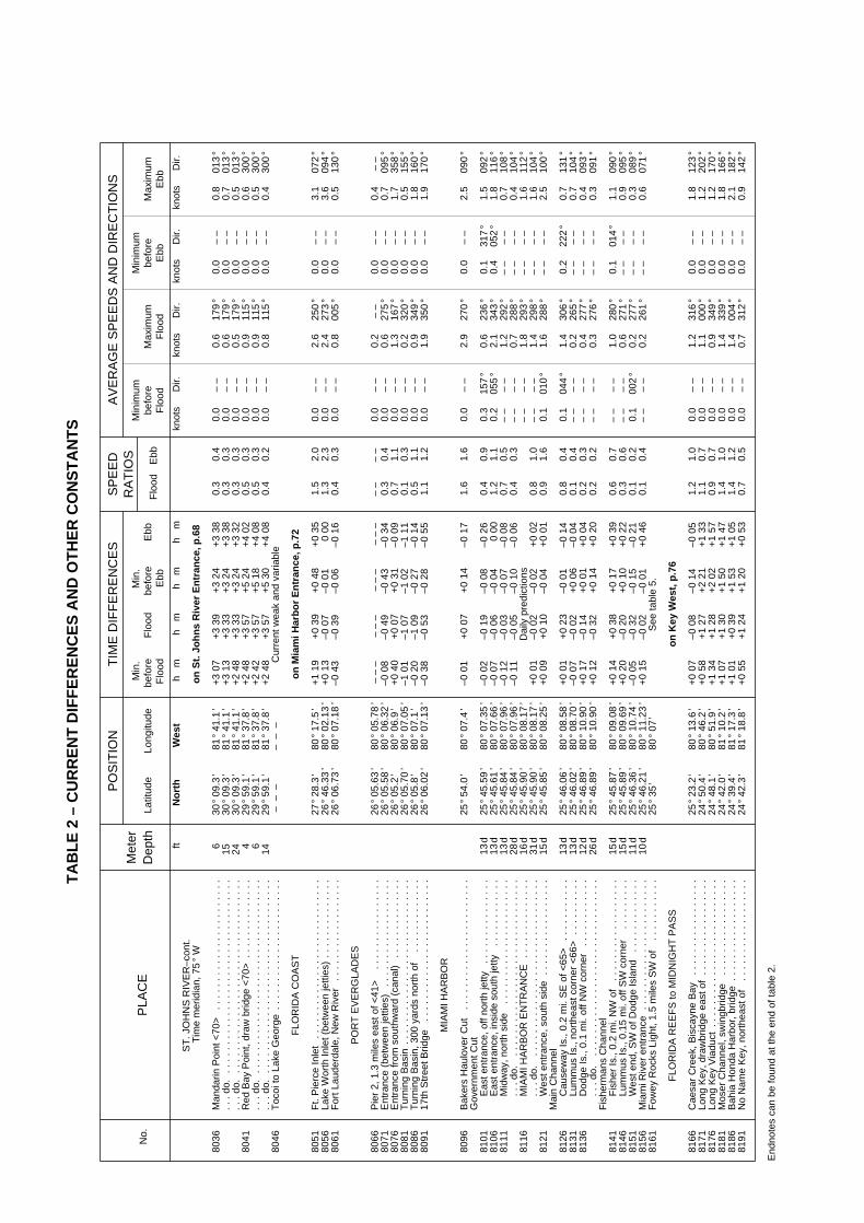
TA
BL
E 2
– C
UR
RE
NT
DIF
FE
RE
NC
ES
AN
D O
TH
ER
CO
NS
TA
NT
S
No.
PLA
CE
Met
erD
epth
PO
SIT
ION
Latit
ude
Long
itude
TIM
E D
IFF
ER
EN
CE
S
Min
.be
fore
Flo
odF
lood
Min
.be
fore
Ebb
Ebb
SP
EE
DR
AT
IOS
Flo
odE
bb
AV
ER
AG
E S
PE
ED
S A
ND
DIR
EC
TIO
NS
Min
imum
befo
reF
lood
Max
imum
Flo
od
Min
imum
befo
reE
bbM
axim
umE
bb
fth
mh
mh
mh
mkn
ots
knot
skn
ots
knot
sD
ir.D
ir.D
ir.D
ir.N
ort
hW
est
ST
. JO
HN
S R
IVE
R–c
ont.
Tim
e m
erid
ian,
75
° W
on
St.
Jo
hn
s R
iver
En
tran
ce, p
.68
8036
Man
darin
Poi
nt <
70>
. . .
. . .
. . .
. . .
. . .
. . .
. . .
. .
630
°09.
3’
81
°41.
1’
+3
07+
3 39
+3
24+
3 38
0.3
0.4
0.0
– –
0.6
179
°0.
0–
–0.
801
3°
. . .
do.
. . .
. . .
. . .
. . .
. . .
. . .
. . .
. . .
. . .
. . .
. . .
.15
30°0
9.3
’ 8
1°4
1.1
’+
3 13
+3
33+
3 24
+3
380.
30.
30.
0–
–0.
617
9°
0.0
– –
0.7
013
°. .
. do
. .
. . .
. . .
. . .
. . .
. . .
. . .
. . .
. . .
. . .
. . .
. . .
2430
°09.
3’
81
°41.
1’
+2
48+
3 33
+3
24+
3 32
0.3
0.3
0.0
– –
0.5
179
°0.
0–
–0.
501
3°
8041
Red
Bay
Poi
nt, d
raw
brid
ge <
70>
. . .
. . .
. . .
. . .
. .
429
°59.
1’
81
°37.
8’
+2
48+
3 57
+5
24+
4 02
0.5
0.3
0.0
– –
0.9
115
°0.
0–
–0.
630
0°
. . .
do.
. . .
. . .
. . .
. . .
. . .
. . .
. . .
. . .
. . .
. . .
. . .
.6
29°5
9.1
’ 8
1°3
7.8
’+
2 42
+3
57+
5 18
+4
080.
50.
30.
0–
–0.
911
5°
0.0
– –
0.5
300
°. .
. do
. .
. . .
. . .
. . .
. . .
. . .
. . .
. . .
. . .
. . .
. . .
. . .
1429
°59.
1’
81
°37.
8’
+2
48+
3 57
+5
30+
4 08
0.4
0.2
0.0
– –
0.8
115
°0.
0–
–0.
430
0°
8046
Toc
oi to
Lak
e G
eorg
e .
. . .
. . .
. . .
. . .
. . .
. . .
. . .
.–
– –
– –
–C
urre
nt w
eak
and
varia
ble
FLO
RID
A C
OA
ST
on
Mia
mi H
arb
or
En
tran
ce, p
.72
8051
Ft.
Pie
rce
Inle
t .
. . .
. . .
. . .
. . .
. . .
. . .
. . .
. . .
. . .
27°2
8.3
’ 8
0°1
7.5
’+
1 19
+0
39+
0 48
+0
351.
52.
00.
0–
–2.
625
0°
0.0
– –
3.1
072
°80
56La
ke W
orth
Inle
t (be
twee
n je
tties
) . .
. . .
. . .
. . .
. . .
26°4
6.33
’ 8
0°0
2.13
’+
0 13
–0 0
7–0
01
0 00
1.3
2.3
0.0
– –
2.4
273
°0.
0–
–3.
609
4°
8061
For
t Lau
derd
ale,
New
Riv
er .
. . .
. . .
. . .
. . .
. . .
. .26
°06.
73’
80
°07.
18’
–0 4
3–0
39
–0 0
6–0
16
0.4
0.3
0.0
– –
0.8
005
°0.
0–
–0.
513
0°
PO
RT
EV
ER
GLA
DE
S
8066
Pie
r 2,
1.3
mile
s ea
st o
f <41
> .
. . .
. . .
. . .
. . .
. . .
26°0
5.63
’ 8
0°0
5.78
’–
– –
– –
––
– –
– –
––
––
–0.
0–
–0.
2–
–0.
0–
–0.
4–
–80
71E
ntra
nce
(bet
wee
n je
tties
) .
. . .
. . .
. . .
. . .
. . .
. . .
26°0
5.58
’ 8
0°0
6.32
’–0
08
–0 4
9–0
43
–0 3
40.
30.
40.
0–
–0.
627
5°
0.0
– –
0.7
095
°80
76E
ntra
nce
from
sou
thw
ard
(can
al)
. . .
. . .
. . .
. . .
. .
26°0
5.2
’ 8
0°0
6.9
’+
0 40
+0
07+
0 31
–0 0
90.
71.
10.
0–
–1.
316
7°
0.0
– –
1.7
358
°80
81T
urni
ng B
asin
. . .
. . .
. . .
. . .
. . .
. . .
. . .
. . .
. . .
. .
26°0
5.70
’ 8
0°0
7.05
’–1
01
–1 0
7–1
02
–1 1
10.
10.
30.
0–
–0.
232
0°
0.0
– –
0.5
155
°80
86T
urni
ng B
asin
, 300
yar
ds n
orth
of
. . .
. . .
. . .
. . .
.26
°05.
8’
80
°07.
1’
–0 2
0–1
09
–0 2
7–0
14
0.5
1.1
0.0
– –
0.9
349
°0.
0–
–1.
816
0°
8091
17th
Str
eet B
ridge
. . .
. . .
. . .
. . .
. . .
. . .
. . .
. . .
.26
°06.
02’
80
°07.
13’
–0 3
8–0
53
–0 2
8–0
55
1.1
1.2
0.0
– –
1.9
350
°0.
0–
–1.
917
0°
MIA
MI H
AR
BO
R
8096
Bak
ers
Hau
love
r C
ut .
. . .
. . .
. . .
. . .
. . .
. . .
. . .
.25
°54.
0’
80
°07.
4’
–0 0
1+
0 07
+0
14–0
17
1.6
1.6
0.0
– –
2.9
270
°0.
0–
–2.
509
0°
Gov
ernm
ent C
ut81
01
Eas
t ent
ranc
e, o
ff no
rth
jetty
. . .
. . .
. . .
. . .
. . .
13d
25°4
5.59
’ 8
0°0
7.35
’–0
02
–0 1
9–0
08
–0 2
60.
40.
90.
315
7°
0.6
236
°0.
131
7°
1.5
092
°81
06
Eas
t ent
ranc
e, in
side
sou
th je
tty .
. . .
. . .
. . .
. .13
d25
°45.
61’
80
°07.
66’
–0 0
7–0
06
–0 0
40
001.
21.
10.
205
5°
2.1
343
°0.
405
2°
1.8
116
°81
11
Mid
way
, nor
th s
ide
. . .
. . .
. . .
. . .
. . .
. . .
. . .
.13
d25
°45.
84’
80
°07.
96’
–0 1
2–0
03
–0 0
7–0
08
0.7
0.5
– –
– –
1.2
292
°–
––
–0.
710
8°
.
. . d
o. .
. . .
. . .
. . .
. . .
. . .
. . .
. . .
. . .
. . .
. . .
28d
25°4
5.84
’ 8
0°0
7.96
’–0
11
–0 0
5–0
10
–0 0
60.
40.
3–
––
–0.
728
8°
– –
– –
0.4
104
°81
16
MIA
MI H
AR
BO
R E
NT
RA
NC
E .
. . .
. . .
. . .
. . .
.16
d25
°45.
90’
80
°08.
17’
Dai
ly p
redi
ctio
ns–
––
–1.
829
3°
– –
– –
1.6
112
°
. .
. do.
. . .
. . .
. . .
. . .
. . .
. . .
. . .
. . .
. . .
. . .
.31
d25
°45.
90’
80
°08.
17’
+0
01–0
02
–0 0
2+
0 02
0.8
1.0
– –
– –
1.4
298
°–
––
–1.
610
4°
8121
W
est e
ntra
nce,
sou
th s
ide
. . .
. . .
. . .
. . .
. . .
. .
15d
25°4
5.85
’ 8
0°0
8.25
’+
0 09
+0
10–0
04
+0
010.
91.
60.
101
0°
1.6
288
°–
––
–2.
510
0°
Mai
n C
hann
el81
26
Cau
sew
ay Is
., 0.
2 m
i. S
E o
f <65
> .
. . .
. . .
. . .
.13
d25
°46.
06’
80
°08.
58’
+0
01+
0 23
–0 0
1–0
14
0.8
0.4
0.1
044
°1.
430
6°
0.2
222
°0.
713
1°
8131
L
umm
us Is
., no
rthe
ast c
orne
r <
66>
. . .
. . .
. . .
.13
d25
°46.
02’
80
°08.
70’
–0 0
7–0
02
+0
06–0
04
0.1
0.4
– –
– –
0.2
265
°–
––
–0.
710
4°
8136
D
odge
Is.,
0.1
mi.
off N
W c
orne
r .
. . .
. . .
. . .
. .12
d25
°46.
89’
80
°10.
90’
+0
17–0
14
+0
01+
0 04
0.2
0.3
– –
– –
0.4
277
°–
––
–0.
409
3°
.
. . d
o. .
. . .
. . .
. . .
. . .
. . .
. . .
. . .
. . .
. . .
. . .
26d
25°4
6.89
’ 8
0°1
0.90
’+
0 12
–0 3
2+
0 14
+0
200.
20.
2–
––
–0.
327
6°
– –
– –
0.3
091
°F
ishe
rman
s C
hann
el81
41
Fis
her
Is.,
0.2
mi.
NW
of
. . .
. . .
. . .
. . .
. . .
. . .
15d
25°4
5.87
’ 8
0°0
9.08
’+
0 14
+0
38+
0 17
+0
390.
60.
7–
––
–1.
028
0°
0.1
014
°1.
109
0°
8146
L
umm
us Is
., 0.
15 m
i. of
f SW
cor
ner
. . .
. . .
. . .
15d
25°4
5.89
’ 8
0°0
9.69
’+
0 20
–0 2
0+
0 10
+0
220.
30.
6–
––
–0.
627
1°
– –
– –
0.9
095
°81
51
Wes
t end
, SW
of D
odge
Isla
nd .
. . .
. . .
. . .
. . .
11d
25°4
6.36
’ 8
0°1
0.74
’–0
05
–0 3
2–0
15
–0 2
10.
10.
20.
100
2°
0.2
277
°–
––
–0.
308
9°
8156
Mia
mi R
iver
ent
ranc
e .
. . .
. . .
. . .
. . .
. . .
. . .
. . .
.10
d25
°46.
21’
80
°11.
23’
+0
15–0
02
–0 0
1+
0 46
0.1
0.4
– –
– –
0.2
261
°–
––
–0.
607
1°
8161
Fow
ey R
ocks
Lig
ht, 1
.5 m
iles
SW
of
. . .
. . .
. . .
. .
25°3
5’
80
°07
’S
ee ta
ble
5.
FLO
RID
A R
EE
FS
to M
IDN
IGH
T P
AS
So
n K
ey W
est,
p.7
6
8166
Cae
sar
Cre
ek, B
isca
yne
Bay
. . .
. . .
. . .
. . .
. . .
. .
25°2
3.2
’ 8
0°1
3.6
’+
0 07
–0 0
8–0
14
–0 0
51.
21.
00.
0–
–1.
231
6°
0.0
– –
1.8
123
°81
71Lo
ng K
ey, d
raw
brid
ge e
ast o
f . .
. . .
. . .
. . .
. . .
. . .
24°5
0.4
’ 8
0°4
6.2
’+
0 58
+1
27+
2 21
+1
331.
10.
70.
0–
–1.
100
0°
0.0
– –
1.2
202
°81
76Lo
ng K
ey V
iadu
ct .
. . .
. . .
. . .
. . .
. . .
. . .
. . .
. . .
.24
°48.
1’
80
°51.
9’
+1
34+
1 28
+2
02+
1 57
0.9
0.7
0.0
– –
0.9
349
°0.
0–
–1.
217
0°
8181
Mos
er C
hann
el, s
win
gbrid
ge .
. . .
. . .
. . .
. . .
. . .
.24
°42.
0’
81
°10.
2’
+1
07+
1 30
+1
50+
1 47
1.4
1.0
0.0
– –
1.4
339
°0.
0–
–1.
816
6°
8186
Bah
ia H
onda
Har
bor,
brid
ge .
. . .
. . .
. . .
. . .
. . .
. .24
°39.
4’
81
°17.
3’
+1
01+
0 39
+1
53+
1 05
1.4
1.2
0.0
– –
1.4
004
°0.
0–
–2.
118
2°
8191
No
Nam
e K
ey, n
orth
east
of
. . .
. . .
. . .
. . .
. . .
. . .
24°4
2.3
’ 8
1°1
8.8
’+
0 55
+1
24+
1 20
+0
530.
70.
50.
0–
–0.
731
2°
0.0
– –
0.9
142
°
End
note
s ca
n be
foun
d at
the
end
of ta
ble
2.

55
APPENDIX C. Notice-to-Mariners issued on December 15, 1998

56
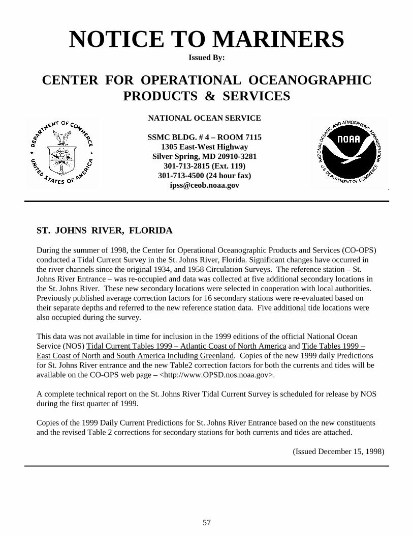
57
NOTICE TO MARINERSIssued By:
CENTER FOR OPERATIONAL OCEANOGRAPHICPRODUCTS & SERVICES
NATIONAL OCEAN SERVICE
SSMC BLDG. # 4 – ROOM 71151305 East-West Highway
Silver Spring, MD 20910-3281301-713-2815 (Ext. 119)
301-713-4500 (24 hour fax)[email protected]
ST. JOHNS RIVER, FLORIDA
During the summer of 1998, the Center for Operational Oceanographic Products and Services (CO-OPS)conducted a Tidal Current Survey in the St. Johns River, Florida. Significant changes have occurred inthe river channels since the original 1934, and 1958 Circulation Surveys. The reference station – St.Johns River Entrance – was re-occupied and data was collected at five additional secondary locations inthe St. Johns River. These new secondary locations were selected in cooperation with local authorities. Previously published average correction factors for 16 secondary stations were re-evaluated based ontheir separate depths and referred to the new reference station data. Five additional tide locations werealso occupied during the survey.
This data was not available in time for inclusion in the 1999 editions of the official National OceanService (NOS) Tidal Current Tables 1999 – Atlantic Coast of North America and Tide Tables 1999 –East Coast of North and South America Including Greenland. Copies of the new 1999 daily Predictionsfor St. Johns River entrance and the new Table2 correction factors for both the currents and tides will beavailable on the CO-OPS web page – <http://www.OPSD.nos.noaa.gov>.
A complete technical report on the St. Johns River Tidal Current Survey is scheduled for release by NOSduring the first quarter of 1999.
Copies of the 1999 Daily Current Predictions for St. Johns River Entrance based on the new constituentsand the revised Table 2 corrections for secondary stations for both currents and tides are attached.
(Issued December 15, 1998)