Last Revision Rev-26 December 8, 2008 meg

1

CURRENT-VIEWING RESISTOR VALIDATION AND APPLICATION Copyright © 1986 - 2008 by Michael E. Gruchalla, All Rights Reserved*

ABSTRACT Current-viewing resistors are common sensors applied in instrumentation systems for direct measurement of system currents. The current-viewing resistor typically comprises a very low resistance placed in series with the conductor to be instrumented where the conductor current is witnessed as the potential developed across the current-viewing resistor. Series inductance in a current-viewing resistor creates a network zero in the response at ω0=R/L. At frequencies above ω0, the impedance of the current-viewing resistor rises due to this inductive component. This results in higher than expected output potentials for a given current, and very high overshoot and ringing in transient signals having spectral content above ω0. Also, the very low value of the current-viewing resistor can result in validation and measurement errors at DC and low frequencies as well due to circulating currents in the reference conductors. Validation and application of the current-viewing resistor and the most common sources of current-viewing resistor measurement error are reviewed.

* This work is continuation of original research begun by the author in 1984. This is an unpublished work of the author. The author welcomes comments and critical review, but this work shall not be distributed or published in any manner without the prior written consent of the author.

1. INTRODUCTION The current-viewing resistor (“CVR”) is a

deceptively-simple sensor. In principle, the current-viewing resistor is simply a low-value resistor. The current of interest is driven through the CVR and the potential across the CVR is recorded. The measured current is then computed simply as I = VCVR / RCVR. The resistance value of the CVR is selected such that the potential developed across the CVR resistance at full current may be considered sufficiently negligible that normal circuit operation is unaffected.

The resistance of typical current-viewing resistors is often quite small ranging from several milliohms to µOhms. This low resistance creates at least two critical issues in the application of the CVR.

One primary concern is series inductance in series with the CVR resistive element. Such inductance can be an inadvertent inductance introduced due to a less-than-optimum implementation of the CVR, or it can be an inherent inductance in the actual CVR sensor.

Series inductance results in a network zero in the frequency response of the CVR at ω0 = RCVR/LCVR. At frequencies above ω0, the impedance of the CVR rises with frequency with a first-order characteristic. This results in the output potential at frequencies above the response zero being higher than would be provided by the CVR resistance alone. The error can be quite substantial, particularly for very low-value CVR devices. It would not be unexpected that errors

AUTHOR’S CVR RESEARCH HISTORY and

MANUSCRIPT-DEVELOPMENT The author has over 35 years experience in the design and implementation of sensors and instrumentation systems. The author’s originalresearch in development of novel CVR elements and best practices in CVR applications was begun in about 1984. The author has worked with T&M Research Products, Inc. (Albuquerque, New Mexico) for many years in the development of novel sensor designs, including CVR devices. T&M Research Products retained the author to develop unique methods to extend the operating range of itsCVR products. This manuscript was expanded to include detailed review of the low-frequency instrumentation effects and the high-frequencyinductive effects of commercial CVR devices and the improvement in frequency response that may be enjoyed with careful design and implementation of device-specific compensating elements.

2

on the order of 1,000 to 10,000 could result where the apparent current appears to be much higher than its true value if the series inductance is not taken into account.

However, often the series inductance is unknown, and it is almost never specified in commercial sensors. As a result, very significant measurement errors can be unknowingly introduced into RF and pulsed current measurements. Therefore, the response characteristics of a CVR must be well understood over the entire spectrum of interest.

The low value of the CVR resistance can also result in instrumentation errors at DC and low frequencies well below any response zero created by series inductance. This is due to parasitic resistance in the overall effective measurement path. Often this parasitic resistance is not obvious resulting in it being overlooked. The effect of this parasitic resistance is to cause the output potential of the CVR to appear higher than that due to the CVR resistance alone. This error too can be quite significant, perhaps as much as a factor of 10 to 1000. However, this error is due to the instrumentation configuration, and is not a characteristic of the CVR sensor.

Both the CVR characteristics and the total instrumentation configuration must be carefully considered to assure accurate CVR measurements.

2. CVR VALIDATION MEASUREMENT A critical element in the application of the CVR is

the accurate characterization of the transfer function, not only at DC, but also over frequency. This can be challenging due to the low resistance of the CVR.

This low resistance value results in low output potentials for currents typically applied in calibration operations. The output levels can be as low as a few nanovolts for very low-value CVR elements. These low output signals require extreme care in both the measurement configuration and the measurement process to assure that noise does not corrupt the calibration process.

The CVR resistance very often is much lower than the resistance of the interconnecting cables utilized in the calibration process. As noted, this can result in parasitic resistance introduced in to the measurement. For very low-value CVR elements, the instrumentation resistance can easily be several orders of magnitude greater than the CVR resistance resulting in very significant measurement errors if proper care is not exercised in the test configuration.

System noise is also typically a limiting factor in the calibration of CVR devices. Again, extreme care is required to assure that neither internal system noise nor external noise, 60Hz noise for example, corrupts the measurements.

The error sources may not always be obvious, and error introduced into the data may not be recognized as error. It is therefore vitally important that those characterizing and utilizing CVR devices thoroughly understand the error sources, have the experience to recognize error-corrupted data, and have the experience to control, or even mitigate the error mechanisms.

2.1 Network-Analyzer Considerations Where the sources of error can be adequately

controlled, the network analyzer is the most convenient instrument for characterizing the CVR transfer function over frequency. The network analyzer provides a very convenient means to collect both magnitude and phase response over quite wide frequency ranges and with a quite wide dynamic range.

Two important parameters of network analyzer measurements are the noise floor and the dynamic range. The signal levels in network-analyzer CVR measurements are expected to be quite low. The fundamental noise of the measurement system will determine the lowest signal levels that may be observed. The dynamic range of the network analyzer system determines how far below the reference power level signals may be observed. For example, the gain of a 100µOhm CVR in a 50-Ohm network analyzer S21 measurement is -108dB. The dynamic range of the measurement system must be greater than 108dB, and a signal level 108dB below the reference level must be substantially above the noise floor.

Although the noise floor and dynamic range are related, these are separate system parameters. Part of the measurement-validation process is to assure that both the measurement-system noise floor and the dynamic range are suitable for the intended measurements.

Although the network analyzer provides a very wide dynamic range in measurements, it is not a low noise instrument in comparison to devices such as a low-noise amplifier (“LNA”).

As noted, the signal levels in CVR measurements can typically be more than 100dB below the reference level. The receiver levels of less than a microvolt can be expected.1

The very low signal levels expected require high-quality materials and extreme care in connector cleanliness and connection. The author uses SMA terminated nominal 1m Andrew FSJ1-50A heliax

1 If the reference level is 0dBm, the receiver power when measuring a 100 µOhm CVR is -108dBm, -138dbW, which is 0.9µV RMS in a 50-Ohm system.

3

instrumentation cables.2 All connectors are lightly cleaned before each mating (simply brushed to remove accumulated debris), and the SMA connectors torqued to 8in-lbs.3

Also, flexing of the source and receiver transmission lines can alter the response by several tenths of a dB at the higher frequencies. This is due to slight changes in the geometry of the line structure, and, for braded-shield materials, changes in the line transfer impedance results due to altering of the shield coverage as the material is flexed. Changes in system parameters as low as 10PPM could introduce measurement errors in these wide-dynamic-range measurements of 100dB or more. Therefore, flexing of the source and receiver lines, particularly between normalization and Test-Article measurement should be minimized.

The use of transmission lines having a solid shield such as heliax or semirigid materials reduces the effects of flexing of the lines, but these are comparatively stiff and may be difficult to apply in all applications. There are also very high-quality transmission-line materials available, but these are typically quite costly, and therefore somewhat less than desirable than the less-costly alternatives, particularly for small laboratories and general laboratory use where it is reasonably expected that the lines will be subjected to substantial handling and abuse, and therefore will have a rather limited lifetime. Heliax and semirigid materials are not only much less costly than other alternatives, but also are easily fabricated and repaired in the user’s laboratory.

The solid-shield materials also provide true 100 percent shield coverage, if the connectors are properly installed. This is a very critical consideration in the wide dynamic-range measurements encountered in CVR measurements.

It is for these reasons that the author typically prefers heliax transmission-lines for most test applications, and particularly for measurements of low-resistance CVR devices.

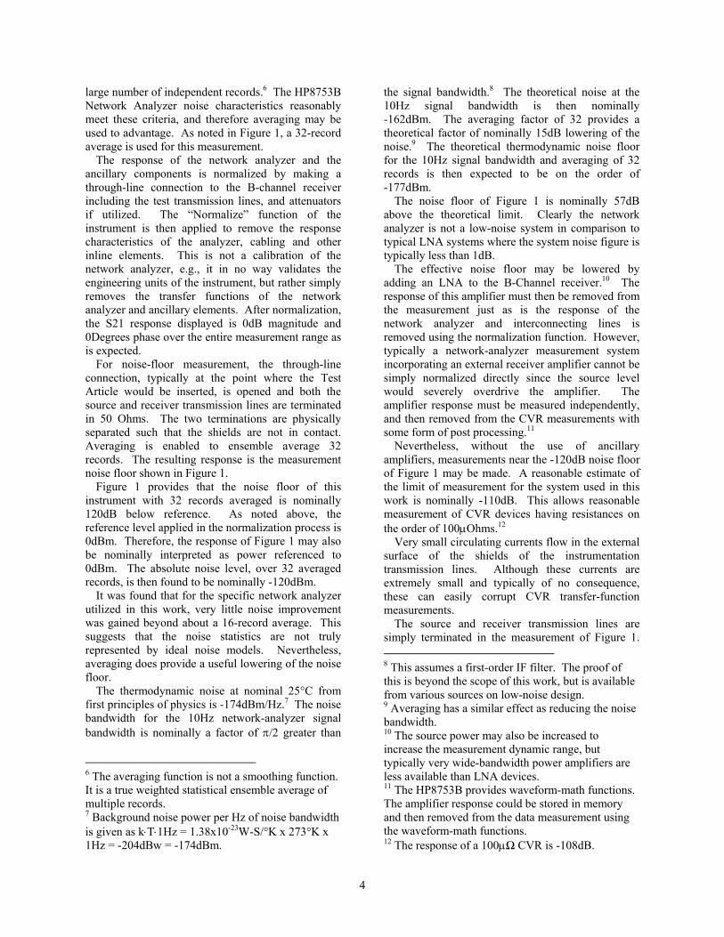
Figure 1 is the noise floor of the HP8735B network analyzer used by the author in this work.4 2 This is a ¼” heliax material having a cutoff frequency of nominally 20GHz and is adequately flexible for use as general-purpose instrumentation cabling. 3 The author has found that a torque of 8in-lbs is a reasonable compromise for both brass and stainless steel SMA connectors even thought 5in-lbs is the recommended torque of brass components. 4 For each measurement, the author disassembles the system, cleans and reconnects all the components, verifies that the un-normalized response is as expected, and normalizes the system response. The

Figure 1. HP8753B Noise-Floor,

0dBm Reference

For this noise-floor measurement, the network analyzer is configured with a standard 6dB resistive power divider at the source port with one output driving the network-analyzer Reference receiver, and the other output driving the B-Channel receiver through the actual transmission lines and other ancillary elements that are to be utilized in the actual Test-Article measurements. The instrument is configured to display S21, e.g., B/R.5 The IF bandwidth is set to 10Hz which is the narrowest bandwidth provided in this instrument.

The source power is set to +6dBm. This results in an input power to the Reference and B-Channel receivers of 0dBm. This establishes 0dBm as the reference power level to both the Reference receiver and the Test-Article input port. Although the network analyzer is typically used to measure transfer functions, e.g., Test-Article output power as a function of input power, its receivers are effectively wide-bandwidth receivers. Therefore, the network analyzer may also be applied to make wide-bandwidth transfer-function power measurements. This could be done by observing the B-Channel signal rather than the S21 (B/R) parameter. However, in the instrument utilized in this work, the averaging function is unavailable for non-ratio measurements.

If the noise is nominally Gaussian, white, ergodic and stationary, the averaging function allows the noise floor to be lowered by ensemble averaging a

author uses this approach to assure that all measurements are repeatable. 5 The author does not utilize the S-Parameter Test Set in CVR measurements in order to minimize any extraneous system loss and to minimize the opportunity for entry of system noise.

4

large number of independent records.6 The HP8753B Network Analyzer noise characteristics reasonably meet these criteria, and therefore averaging may be used to advantage. As noted in Figure 1, a 32-record average is used for this measurement.

The response of the network analyzer and the ancillary components is normalized by making a through-line connection to the B-channel receiver including the test transmission lines, and attenuators if utilized. The “Normalize” function of the instrument is then applied to remove the response characteristics of the analyzer, cabling and other inline elements. This is not a calibration of the network analyzer, e.g., it in no way validates the engineering units of the instrument, but rather simply removes the transfer functions of the network analyzer and ancillary elements. After normalization, the S21 response displayed is 0dB magnitude and 0Degrees phase over the entire measurement range as is expected.

For noise-floor measurement, the through-line connection, typically at the point where the Test Article would be inserted, is opened and both the source and receiver transmission lines are terminated in 50 Ohms. The two terminations are physically separated such that the shields are not in contact. Averaging is enabled to ensemble average 32 records. The resulting response is the measurement noise floor shown in Figure 1.

Figure 1 provides that the noise floor of this instrument with 32 records averaged is nominally 120dB below reference. As noted above, the reference level applied in the normalization process is 0dBm. Therefore, the response of Figure 1 may also be nominally interpreted as power referenced to 0dBm. The absolute noise level, over 32 averaged records, is then found to be nominally -120dBm.

It was found that for the specific network analyzer utilized in this work, very little noise improvement was gained beyond about a 16-record average. This suggests that the noise statistics are not truly represented by ideal noise models. Nevertheless, averaging does provide a useful lowering of the noise floor.

The thermodynamic noise at nominal 25°C from first principles of physics is -174dBm/Hz.7 The noise bandwidth for the 10Hz network-analyzer signal bandwidth is nominally a factor of π/2 greater than

6 The averaging function is not a smoothing function. It is a true weighted statistical ensemble average of multiple records. 7 Background noise power per Hz of noise bandwidth is given as k⋅T⋅1Hz = 1.38x10-23W-S/°K x 273°K x 1Hz = -204dBw = -174dBm.

the signal bandwidth.8 The theoretical noise at the 10Hz signal bandwidth is then nominally -162dBm. The averaging factor of 32 provides a theoretical factor of nominally 15dB lowering of the noise.9 The theoretical thermodynamic noise floor for the 10Hz signal bandwidth and averaging of 32 records is then expected to be on the order of -177dBm.

The noise floor of Figure 1 is nominally 57dB above the theoretical limit. Clearly the network analyzer is not a low-noise system in comparison to typical LNA systems where the system noise figure is typically less than 1dB.

The effective noise floor may be lowered by adding an LNA to the B-Channel receiver.10 The response of this amplifier must then be removed from the measurement just as is the response of the network analyzer and interconnecting lines is removed using the normalization function. However, typically a network-analyzer measurement system incorporating an external receiver amplifier cannot be simply normalized directly since the source level would severely overdrive the amplifier. The amplifier response must be measured independently, and then removed from the CVR measurements with some form of post processing.11

Nevertheless, without the use of ancillary amplifiers, measurements near the -120dB noise floor of Figure 1 may be made. A reasonable estimate of the limit of measurement for the system used in this work is nominally -110dB. This allows reasonable measurement of CVR devices having resistances on the order of 100µOhms.12

Very small circulating currents flow in the external surface of the shields of the instrumentation transmission lines. Although these currents are extremely small and typically of no consequence, these can easily corrupt CVR transfer-function measurements.

The source and receiver transmission lines are simply terminated in the measurement of Figure 1. 8 This assumes a first-order IF filter. The proof of this is beyond the scope of this work, but is available from various sources on low-noise design. 9 Averaging has a similar effect as reducing the noise bandwidth. 10 The source power may also be increased to increase the measurement dynamic range, but typically very wide-bandwidth power amplifiers are less available than LNA devices. 11 The HP8753B provides waveform-math functions. The amplifier response could be stored in memory and then removed from the data measurement using the waveform-math functions. 12 The response of a 100µΩ CVR is -108dB.

5

As noted, the shields at the terminations are not connected, e.g., the cables were each terminated and allowed to lay separated from each other.

If the shields are connected, even though the cables are competently terminated, the shield circulating currents will introduce artifacts into the measurement. This is most obvious in the noise-floor measurements.

This is easily demonstrated by clamping together the shields of the connectors of the terminated lines in the noise-floor measurement configuration of Figure 1. This then allows the shield currents on the outside of the source transmission line to flow on the shield of the B-Channel receiver line. Some small part of the receiver shield current escapes into the interior of the receiver line due to the transfer impedance of the receiver transmission line creating artifacts in the received signal. 13 Figure 2 shows the noise-floor measurements with the source and receiver shields connected at the line terminations.

Figure 2. Noise-Floor Measurement with

Shields Connected

Comparing Figures 1 and 2, it is seen that simply connecting the source and receiver shields together in the noise-floor measurement with both transmission lines independently competently terminated results in the introduction of substantial signal components, primarily at the lower limits of the measurement. The noise floor is increased by about 30dB at 300kHz.

The shields of the source and receiver transmission lines will typically be intimately connected at the Test Article. Therefore, the response of Figure 2 is 13 Transmission-line transfer impedance of a terminated line is simply the ratio of the voltage developed at the center conductor of the line to the line shield current.

the true noise floor of the measurement system. Acceptably-accurate measurements may be made where the signal at the measurement frequency is least 10dB above this noise floor at that frequency, but a minimum 20dB margin is a more-preferred margin.

Another measurement-configuration issue that must be managed in the CVR measurement is the mismatch in impedances between the characteristic impedance of the network analyzer, nominally 50 Ohms in this work, and the CVR impedance.

Typically, a network analyzer does not present with accurate matched source and receiver impedances. Often the specified VSWR could be as high as 2:1.

If the CVR is simply driven directly from the source, and the output signal delivered directly to the receiver, VSWR ripple would result if the source and receiver impedances are substantially different from the impedance of the interconnecting transmission lines, This effect will be most noticeable at high sensitivities, e.g., 1dB/Division, but in general will be acceptable at low sensitivities such as 20dB/Division. Also, a gain error would result if the source and receiver impedances are substantially difference from that expected.

It is typically infeasible to design effective matching networks such as minimum-loss pads or true transformers due to the extremely low-impedance expected of typical CVR devices and the wide measurement bandwidth.

The author applies a somewhat unconventional means to accommodate the impedance mismatch. Rather than attempting to actually match the network analyzer to the CVR load, the author simply assures that the impedances presented to the instrumentation transmission lines intimately at the Test Article are very nearly matched impedances, and that matched impedances are also presented to the Test Article.

This serves two purposes. First, since the source and load impedances are accurately known, the CVR response may be computed analytically and meaningfully compared to the measured response. Secondly, multiple reflections in a transmission line, which will result in the classic VSWR ripple in the network response, are eliminated if each transmission line is terminated at least one end.14

The author adds an attenuator to both the source transmission line and the receiver transmission line immediately at the Test Article. The value of these attenuators is a tradeoff between minimizing VSWR artifacts and maximizing noise-limited sensitivity of the measurement. The author typically utilizes 10dB attenuators on both the source and receiver 14 This is reviewed in more detail below.

6

transmission lines with these placed intimately at the Test Article. This of course has the effect of both reducing the source power by 10dB, and attenuating the output signal by 10dB. An S-Parameter test set could also be utilized with full two-port S-Parameter calibration to eliminate the effects of the measurement system. However, the test set can introduce additional path loss and noise, and S-Parameter test sets are not always available. The author has found that the procedure of adding source and receiver attenuators is adequate for the majority of CVR verification applications.

Although the absolute noise floor is unchanged with the addition of the two 10dB attenuators, the dynamic range of the measurement is reduced by 20dB. This reduction in dynamic range may be accommodated by increasing the source power by nominally 20dB.

The maximum source power of the HP8753B is +25dBm. A 20dB attenuator must be added to the Reference-Channel receiver path to prevent overloading the Reference receiver when the source power is set to +25dBm. With the 20dB attenuator added to the Reference path, and the two 10dB attenuators added to the Test-Article path, the system is then normalized to remove the effects of these added elements. This test configuration allows the dynamic-range effect of the Reference and Test-Article attenuators to be reasonably accommodated.

Where increased sensitivity is needed, one of both of the Test-Article attenuators may be removed and the response observed.15 If the resulting VSWR ripple is acceptable for the specific measurement application, the attenuators may be removed and the response reference level adjusted for the +20dB change in the drive level presented to the Test Article.

Also, if the attenuators are removed, it should be verified that the attenuator transfer functions are adequately ideal for the desired measurement accuracy. In may be necessary to remove the attenuator transfer-function response from the measurements using either some form of waveform math or in post processing. 16

Figure 3 is the response of the 10dB attenuators utilized in this work. The data of Figure 3 is the 15 With the source power set at the maximum level to achieve maximum dynamic range, nominally 20dB will be required in the Test-Article path to prevent overdriving the Receiver in the normalization process. 16 Many network analyzers provide some degree of native mathematical functions that may allow corrections to be made within network analyzer itself eliminating the need for additional post processing.

response of the two 10dB attenuators used in this work connected in series to provide a total 20dB attenuation in the measurement path.

Figure 3. Dual 10dB Attenuator Response

Figure 3 shows that over the measurement range the attenuator magnitude response is almost ideal with precisely 20dB attenuation flat within much better than 0.1dB and the phase is almost ideally zero degrees. Therefore, the actual transfer function of these attenuators need not be explicitly removed if the attenuators are removed to achieve greater dynamic range. Only the reference level need be corrected by +20dB since removing the two 10dB attenuators increases the drive to the Test Article by 10dB and increases the signal to the Receiver by 10dB.

The overall dynamic range of the HP8753B instrument utilized in this work is shown in Figure 4.

Figure 4. Maximum HP8753B Dynamic Range

It is important to understand that Figure 4 provides the system dynamic range. Specifically, Test Articles having gains somewhat above -140dB, on the order

7

of -130dB, may be accurately characterized. But, the noise level of -140dB in Figure 4 cannot be interpreted as the absolute noise-floor power. This method of extending the dynamic range does not alter the overall noise performance of the system.

To compute the absolute noise-floor power in Figure 4, the actual power delivered to the B-Channel receiver must be considered. In Figure 4, the source power is set to +25dBm. The system power divider introduces 6dB loss. Therefore, the power delivered to the Test Article with source attenuator removed is +19dBm. Also, removing the B-Channel receiver attenuator increases the power delivered to the B-Channel receiver by 10dB. Therefore, removing the two Test-Article attenuators results in an effective +20dB “gain” in the system response. Removing this 20dB gain from the data of Figure 4, the absolute noise floor is found to be nominally -119dBm. This agrees almost precisely with the noise-floor measurement of Figure 2.

These results of Figure 2 and Figure 4 show that the noise floor of the measurement system utilized in this work is nominally -120dBm, and the maximum available dynamic range is nominally 140dB. This allows characterization of CVR devices as low as nominally 10µOhms with a 10dB noise margin without the need for any ancillary equipment such as LNA devices. If a suitable LNA is added to the B-Channel receiver path, the noise floor may be theoretically reduced by at least 50dB, and the dynamic range increased to nominally 190dB.

2.2. CVR Network-Analysis Measurement Model

The use of a network analyzer is made problematic by the very low resistance of the typical CVR. A very accurate model of the network-analysis configuration must be developed, and very accurate implementation is necessary to achieve accurate results.

A typical network-analysis model used for CVR validation and calibration is shown in Figure 5.17

The model of Figure 5 comprises a source of potential 2VS and source impedance RS driving a coaxial transmission line of characteristic impedance Z0S. The transmission-line segment has some center-conductor and shield resistance as noted. The source potential of 2VS results in a potential of VS across a matched load assuming the transmission-line resistances are negligible. This potential VS is the network-analyzer reference potential and the

17 The source and receiver attenuators reviewed above are simply included in this model as elements of the source and receiver respectively.

potential that would normally be delivered to the matched load in a traditional network analysis. However, in measurements were the load is not matched, as in this analysis where the CVR impedance is very low in comparison to the system characteristic impedance, the potential applied to the CVR will be very much lower than VS.

Figure 5. CVR Network-Analysis Model

When the network-analysis source is driven into the low impedance of the CVR, it is effectively a current source with the excitation current equal to 2VS / RS. But, to achieve accurate results, the model must be well understood to assure accurate interpretation of the data, and extreme care must be applied in the implementation and execution of the measurements.

Referring to Figure 5, the source transmission line drives the CVR under test. The potential developed across the CVR is collected by a second coaxial transmission line of characteristic impedance Z0R to the receiver of load impedance RR. Center-conductor and shield resistance is also noted in the receiver transmission-line segment.

In typical practice, Z0S=Z0R=Rs=RR to provide accurate source and receiver impedance matching.

The two transmission lines are not matched at the CVR. As noted, this can result in unwanted multiple reflections in the measurements. In the model, the source and receiver are defined to provide perfect match to the transmission lines. As referenced above, in general, a transmission line need only be terminated at one end to eliminate multiple reflections. This however may not be obvious.

Consider a signal launched at the source and communicated to the CVR. At the CVR, the majority of the launched power is reflected back to the source. If the source impedance accurately matches the characteristic impedance of the source transmission line, this reflected signal will be perfectly terminated and no power will be reflected back toward the CVR even though the source transmission line is severely mismatched at the CVR.

Similarly, adding a suitable attenuator to the source transmission line at the CVR effectively forward

8

terminates the source preventing multiple reflections even if the load is not well matched.18

Any power launched into the receiver transmission-line segment at the CVR will also be perfectly terminated where the receiver impedance matches the characteristic impedance of the receiver transmission-line segment. Adding an attenuator in the receiver transmission line at the CVR also prevents multiple reflections where the receiver impedance is not well matched.

Matching of the characteristic impedances of transmission-line segments in this manner therefore effectively eliminates multiple reflections. But, care must still be applied in the interpretation of the measurements. And, the signal developed across the CVR must be faithfully communicated to the receiver.

The CVR presents effectively as a near short-circuit. This results in a current being driven into the CVR being determined by the source potential, e.g., 2VS, the source impedance RS, and the source transmission-line center-conductor and shield resistances.

The important fact to note is that the driving potential is the actual equivalent source equivalent potential 2VS, and is not the matched reference potential VS that would be presented to a matched load. Using the matched potential rather than the equivalent source potential will result in a +6dB measurement error, e.g., the measured CVR resistance will appear a factor of two higher than its actual value.

2.3. CVR Low-Frequency Measurement Model At low frequencies, the transfer impedance of the

coaxial feed lines is effectively the shield resistance. As a result, the shield current is not constrained to equal the center-conductor current. This results in a parasitic resistance in series with the CVR.

Figure 6 is the low-frequency measurement model showing the various currents. The coaxial transmission-line shield is modeled with an inner and outer resistance with the shield current flowing in the entire shield cross-section. This current flowing in the shield at low frequencies results in a shield potential between the ends of the transmission-line

18 Using 50-Ohm 10dB attenuators, the impedance looking into the attenuator loaded with a short is 41 Ohms, and 61 Ohms if loaded with an open circuit. This results in a worse-case VSWR of 1.22:1. Although this is not a particularly low VSWR, it is typically an acceptable tradeoff between noise and VSWR ripple.

segment. These shield potentials compromise the measurement of the CVR potential.

Figure 6. Low-Frequency Measurement Model

Examining Figure 6, it is seen that the source current is delivered to the CVR. A small portion of the source current is delivered to the receiver. This error should be considered, but as shown below, it is typically insignificant in most typical applications.

The current delivered to the CVR returns via the shields of the source and receiver transmission lines and the interconnected grounds. This results in the shield resistances appearing in series with the CVR. Figure 7 shows the equivalent circuit at low frequencies.

Figure 7. Low-Frequency Equivalent Circuit

Comparing Figures 4 and 5 it is seen that these are equivalent where the shield resistances have simply been separated from the transmission-line model. These shield resistances are shown in Figure 7 in the CVR return path to clearly show the effect of the shield resistance. Examining this return path in Figures 4 and 5, it is seen that the return paths of Figure 7 are identical to that of Figure 6.

The potential VR delivered to the receiver may be computed by inspection of Figure 7:

( ) ⋅⎥⎦

⎤⎢⎣

⎡++++

⋅⋅=

SCCSSHRSHSCVRCCSS

sR

RRRRRRR

VV

//(//1

2

( ) ⎟⎟⎠

⎞⎜⎜⎝

⎛+

⋅+CCRR

RSHRSHSCVR RR

RRRR // (1)

Equation 1 is the exact solution, but due to its

complexity, the critical parameters are not clearly

9

obvious. It is useful to examine the approximate response making several assumptions to reduce the complexity of the expression.

The center-conductor resistances are typically expected to be very much smaller than the characteristic impedance of the measurement system. For example, the typical center-conductor resistance for a 50-Ohm system would be expected to be less than perhaps 0.05 Ohm. Therefore, to a first-order estimate the center-conductor resistance may be ignored. This will result in less than about a 0.1 percent error (~0.06dB).

It would also be expected that the length of the source and receiver transmission lines would be roughly equal for a typical network analysis. Therefore, the approximation RSHS = RSHR ≡ RSH may be made.

Appling these approximations, the model of Figure 8 results. The shield resistances are combined as a single resistance to system ground. In this model, the effect of the shield resistance is very easily seen as a resistance directly in series with the CVR.

Figure 8. Simplified Equivalent Low-Frequency

CVR Measurement Circuit

The receiver potential may again be written by inspection of Figure 8 applying the noted approximations:

⎟⎟⎠

⎞⎜⎜⎝

⎛ +⋅≅

S

SHCVRsLFR R

RRVV

2/12)( (2)

Examining Figure 8, it is seen that the potential at

the receiver is the potential developed across the series combination of the CVR resistance and one-half the shield resistance. Although the shield resistance is expected to be much lower than the center-conductor resistance, and very much lower than the system characteristic impedance, it will typically be substantial compared to the CVR resistance.

For example, a reasonable estimate for the shield resistance including connection resistance would be on the order of several milliohms. Consider a 100µOhm CVR. If the shield resistance were only

one milliohm, the equivalent parasitic resistance presenting in series with the CVR would be 500µOhms. The response observed would be about 16dB higher than that of the CVR alone.

The transfer-function gain of the CVR in Figure 8 may be expressed in dB by dividing Equation 2 by VS and expressing the voltage ratio in dB.

⎟⎟⎠

⎞⎜⎜⎝

⎛ +=≅

S

SHVCR

S

CVRLF R

RRLog

VV

LogG2

2020 1010 (3)

It should again be noted that the term VS is the

network analysis reference potential, e.g., the potential that is delivered by the source to a matched load.

If the measured gain in the model of Figure 8 is used to compute the CVR impedance, and the shield resistance is ignored, as is the case where this effect of the shield resistance is not understood or simply not recognized, the CVR resistance will appear in this example to be 600µOhms rather than the actual value of 100µOhms.

It may seem in Figure 8 that the error caused by the shield resistance could be eliminated by simply tying the lower terminal of the CVR directly to “ground” thereby shunting the shield resistance. This however is not feasible since the ground terminals of the source, receiver and CVR would have to be connected together with zero-resistance connections.

In the case of DC and low-frequency measurements, e.g., 60Hz, the shield-resistance error may be eliminated by utilizing an isolated or “floating” receiver where the ground connections to the receiver are removed, for example by using a battery-operated digital millimeter as the receiver. An isolated receiver configuration is shown in Figure 9.

Figure 9. Isolated Receiver

The actual CVR terminals are shown as terminals A and B in Figure 9. The model of Figure 9 shows that isolating the receiver from ground results in a four-wire connection to the CVR where the source shield current (I1) is forced to identically equal the source center-conductor current (Is). Similarly, the

10

receiver shield current is forced to equal the receiver center-conductor current. The significance of this model is that no CVR return current flows in the receiver shield path.

The configuration of Figure 9 effectively provides Kelvin sensing of the CVR.19 Specifically, all current delivered to the CVR on the source center conductor is returned on the source shield. The only current allowed to flow in the receiver shield is the receiver load current.

Where the receiver resistance is very large compared to the CVR resistance, and the receiver center conductor and shield resistances are very small compared to the receiver impedance, the potential at the receiver load resistance RR is nominally equal to the potential developed at the CVR terminals A and B.20

The same result achieved by isolating the receiver may be achieved by isolating the source. However, in typical applications of CVR devices, it is often impractical to isolate the source. But, as reviewed below, there are several approaches to effectively isolate the receiver. Accordingly, the model of Figure 9 is typically the most practical configuration in actual applications.

2.4. CVR RF Measurement Model Although DC and low-frequency measurements

may be made effectively with an isolated receiver or Kelvin bridge, RF measurements will typically be constrained to a configuration such as shown in Figure 6 above.

The error due to the shield resistances may again be eliminated by forcing the source shield current to be equal to the center-conductor current. This condition is shown in the RF model of Figure 10.

Figure 10. CVR RF Measurement Model

19 A Kelvin bridge is typically utilized to very accurately measure the DC resistance of the CVR. 20 For very accurate metrology, the loading effect of the receiver circuit on the CVR and the voltage divider effect of the receiver center-conductor and shield resistances in series with the load resistance would be considered.

If the shield current I1 is forced to equal the center-conductor current IS, the current between the source and receiver grounds is then forced to zero. This is seen by inspection of Figure 10.

Current IS is delivered to the CVR. Some small current IR flows toward the receiver, and the remaining source current flows through the CVR. Since the source shield currents are forced to equal the center-conductor currents, the current delivered to the receiver resistance must return via the shield of the receiver transmission line back to the CVR as -I2. The current I1 returning on the shield of the source transmission line is then identically equal to the source current. Therefore, no current is available to flow in the ground connection between the source and receiver.

The equivalent circuit of the model of Figure 10 is shown in Figure 11.

Figure 11. RF Model Equivalent Circuit

Examining Figure 11, it is easily seen that if the source center-conductor and shield currents are constrained to be equal, the inter-ground current must be identically zero.

Also examining Figure 11, it is seen that the combination of the receiver resistance in series with the center conductor and shield resistances is simply in parallel with the CVR. Where the transmission-line resistances are very small with respect to the receiver resistance, effectively the entire CVR potential appears across the receiver resistance. And, where the receiver resistance is very much larger than the CVR resistance, the parallel combination of the CVR in parallel with the receiver resistance is effectively equal to the CVR resistance. Therefore, the receiver resistance loading the CVR is negligible, and the receiver potential is a reasonably-faithful representation of the CVR potential.

This constraint of forcing the shield current to equal the center-conductor current is automatically provided at frequencies where the transmission line operates as a true transmission line. In effect, the transmission-line properties effect an isolated source and an isolated receiver by forcing any current between the source and receiver grounds to zero.

11

Using the same approximations applied above, the CVR potential and the transfer-function gain may be computed by inspection of Figure 11.

⎟⎟⎠

⎞⎜⎜⎝

⎛⋅≅

S

VCRsHFR R

RVV 2)( (4)

⎟⎟⎠

⎞⎜⎜⎝

⎛=≅

S

VCR

S

CVRHF R

RLog

VV

G2

20 10 (5)

210 20

SG

CVRR

RHF ⋅

≅ (6)

Where the sources of error are eliminated,

Equation 5 provides the gain expected for a specific CVR resistance, and Equation 6 provides the CVR resistance from a measured gain.

3. Practical CVR Measurements Several CVR constructions were characterized by

the author do demonstrate the concepts reviewed in this work. The response data of each of these devices is presented and briefly discussed.

3.1 Simple Resistor CVR A very simple CVR was constructed using a

10-Ohm, 5%, thick-film, 1206 surface-mount resistor. A test fixture was fabricated by cutting small slot through the shield and dielectric to the center conductor of a section of UT-141-50 50-Ohm semirigid coaxial transmission line. This fixture was connected to the HP8753B Network Analyzer configured to measure S21. The slot in the line caused no noticeable spurious responses to the 3GHz measurement limit of the analyzer. The response of this fixture was normalized using the network analyzer normalization function to remove the magnitude and phase response of the fixture and interconnecting feed lines.

The 10-Ohm 1206 surface-mount resistor was set in the slot in the transmission line and connected between the shield and center conductor soldering the terminals of the 1206 package directly to the shield and center conductor respectively to provide minimum length in the configuration. It is estimated that the leakage inductance of this simple configuration is nominally 1nH to 2nH.

The DC value of the resistor was measured to be 10.5 Ohms. The response of this very simple CVR is shown in Figure 12.

Examining Figure 12, it is seen that the low-frequency response is -10.6dB. The value computed from Equation 5 is -7.5dB. This error is due to the

failure of the approximations made to arrive at Equation 5. Specifically, it was approximated that the CVR resistance is negligibly small in comparison to the system characteristic impedance. This is not true for a 50-Ohm system impedance and the 10.5-Ohm CVR resistance of this example.

Figure 12. Response of 10-Ohm 1206 Resistor

An exact solution must be computed by inspection of Figure 11.21

( ) ⎟⎟⎠

⎞⎜⎜⎝

⎛+

=ΩRCVRS

RCVRSR RRR

RRVV

////

25.10 (7)

( ) ⎟⎟⎠

⎞⎜⎜⎝

⎛+⋅

=ΩRCVRS

RCVR

RRRRR

LogG//

//2205.10 10 (8)

Applying the more exact Equation 8, the expected

response based on the resistance value measured at DC is -10.6dB. This now agrees well with the measured data.22

The nominal 1/2dB peak-to-peak magnitude ripple seen above 20MHz is VSWR ripple. Even with the 10dB attenuators at the source and receiver lines, the match is not perfect, and at the 1dB/Division sensitivity, the effect of the impedance mismatch is easily seen. Accordingly, some small amount of VSWR ripple is not uncommon. This could be reduced with more careful design of the fixture and increased attenuation at the Test-Article ports.

21 The transmission-line resistances are not included in this derivation since these are negligibly small in comparison to 50 Ohms. 22 The same result is found if the equivalent Thevenin source impedance of 25 Ohms is used to compute the CVR potential.

12

This specific example is included in this work to demonstrate how easily errors can be accidentally introduced into CVR measurements. Both the calibration and application models must be carefully designed and well understood, the paths of all the circulating currents must be well understood and controlled, and equally important is that any assumptions made must always be validated against each application to assure those assumptions are valid for that specific case.

Both the magnitude and phase response shown in Figure 12 are reasonably flat to about 300MHz. Above 300MHz, the magnitude response shows a rising response. This is due to the series inductance of this very simple construction. This rising response is a network zero at nominally 1.2GHz.23 This response corresponds to a series inductance of nominally 1.6nH.24

This simple CVR would provide faithful response to currents having frequency components below about 300MHz. However, if a 3GHz current were to be viewed, the indicated current would be a factor of about 2.2, 7dB, higher than the actual current.

Similarly, if a square current pulse having a nominal 100ps transition time were measured, the transition edge of the CVR signal would exhibit about a factor of 2.2 overshoot even though no such overshoot is present in the current signal measured.

These artifacts are a result of the leakage inductance of this very simple CVR element. And, if the element resistance were reduced, the effect of this inductance would be enhanced. For example, if a 1-Ohm 1206 resistor were installed in the same manner, the leakage inductance would be expected to be effectively the same since the inductance is a function of the physical geometry. The zero frequency would then move to nominally 60MHz, and the error for a 3GHz current would be nominally a factor of 20, and the overshoot for the 100ps transition-time pulse would also be a factor of 20.

An additional important but subtle feature of the response of Figure 12 is that the phase response is flat at zero degrees to the break frequency, and then breaks up and levels at nominally 45 degrees above the break frequency. If the response were a true network zero, the phase would level at 90 degrees. The fact that the phase is not 90 degrees shows that the 1206 resistor CVR is not a true first-order system. 23 This is estimated at the +3dB frequency by assuming a nominally-accurate first-order response. 24 This response is computed from the 1.2GHz +3dB frequency and the equivalent resistance of the 10.5-Ohm resistor in parallel with the 50-Ohm source and receiver resistances, or about a 7.4-Ohm equivalent resistance.

If this simple resistor CVR were to be used for measurements above 300MHz, not only would correction in the magnitude response be required, but phase correction would also be necessary. This could be provided by developing an accurate analytical model of the resistor CVR from its response of Figure 12, and than applying a complex deconvolution algorithm to remove the response of the CVR from measured data.

A network zero as seen in the response of Figure 12 can be a source of serious error. If the spectral content of the instrumented signal is well below this response zero, the CVR response will be a true representation of the current. However, often the spectral content of the instrumented signal is unknown. If the current signal contains spectral content above the response zero, the CVR response will not faithfully report the current signal.

CVR devices are very often applied in time-domain measurements. Therefore, it is useful to briefly examine in some detail the effect of CVR series inductance on the time-domain response of the CVR.

Figure 13 is the response of a 1-Ohm 1206 surface-mount thick-film resistor mounted in the UT-141 test fixture described above for the 10-Ohm resistor characterization of Figure 12.

Figure 13. Response of 1-Ohm 1206 Resistor

As with the 10-Ohm resistor, this resistor is mounted by soldering its electrodes directly to the transmission-line center conductor and shield respectively providing a minimum-length connection to the resistor. Since inductance is a function of the geometry, the inductance of this 1-Ohm resistor is expected to also be on the order of 1ηH to 2ηH.

The resistance value after installation was measured as 1.01 Ohms. Applying the exact expression of Equation 8, it is found that the expected

13

gain for this 1.01-Ohm CVR in a 50-Ohm system is -28.2dB.

The magnitude response in Figure 13 is flat below the response zero, and the phase is zero degrees. Therefore, in this region from DC to nominally 10MHz, the response of this simple resistor CVR is purely resistive. Marker 1 shows the gain in the resistive region to be -28.2dB. This is the gain expected based on the DC resistance value measured. Marker 2 shows the +3dB frequency to be nominally 120MHz. The equivalent series inductance is found to be nominally 1.3ηH which agrees reasonably with the value computed above for the 10.5-Ohm resistor.

Above 120MHz the gain breaks up indicating a zero-type response. The magnitude rises at nominally 20dB/Decade above 120MHz implying a first-order zero response. At nominally 20MHz the phase begins rising also indicating a response zero. The frequency where the gain increases 3dB is nominally 120MHz. For a first-order system, the phase should be 45 Degrees at the +3dB frequency. However, the phase is actually 49 Degrees. Also, as with the 10.6-Ohm resistor example, the phase does not reach 90 Degrees as expected of a first-order system. Accordingly, this 1-Ohm CVR example is not quite an ideal first-order system. Nevertheless, it is adequately close to first order that it may be reasonably approximated by a first-order model for the majority of applications where such a simple CVR may be utilized.

The frequency response of Figure 13 suggests that the time-domain response will exhibit peaking for signals having spectral components above about 100MHz. The time-domain response was collected using a tunnel-diode pulse source having a nominal 30ps transition time and an HP54510 digitizing oscilloscope having a minimum 300MHz equivalent analog bandwidth.

The response of the pulse source is shown in Figure 14.

Figure 14. Response of Tunnel-Diode Source

This source and oscilloscope have modestly good response characteristics showing a smooth transition and reasonably low overshoot and ringing. The 10%-90% transition time is seen to be nominally 900ps. Assuming this digital oscilloscope digital processing reasonably approximates a first-order

analog response, a 900ps rise time corresponds to a first-order bandwidth of nominally 388MHz.25 This is sufficient to examine the time-domain response of the 1-Ohm resistor CVR.

Figure 15 shows the response of the 1-Ohm resistor to the 30ps pulse.

Figure 15. Time-Domain Response of

1-Ohm 1206 Resistor

As expected, there is substantial overshoot as well as slight ringing. However, these data are deceiving. It should be noted specifically that the transition time is on the order of 700ps. This corresponds to a bandwidth of 500MHz. But, the oscilloscope bandwidth was found to be 388MHz in Figure 14. It appears that the oscilloscope is responding faster than it is capable, or that by some unknown mechanism has greater bandwidth when measuring the CVR than when measuring the source. Also, the data of Figure 15 could be misinterpreted to imply that the 1-Ohm CVR has a bandwidth of at least 500MHz. Of course, both of these observations must be incorrect.

If the oscilloscope analog response is nominally first order, as Figure 14 reasonably suggests, it will act as an integrator for spectral components above its bandwidth. The 30ps rise time of the source corresponds to a bandwidth of nominally 12GHz. Figure 13 shows that there will be little attenuation of spectral components above 3GHz. Therefore, the transition of the 30ps pulse would effectively pass the CVR with little degradation. A peak overshoot roughly equal to the peak level in Figure 14, or on the order of 250mV, would be expected. But, the overshoot seen in Figure 15 is only ~12mV. The 30ps transition of the pulse has been roughly integrated by the oscilloscope, and the transition seen in Figure 15 is not a first-order rise time, but rather a rough integral of the 30ps rise time.

The 12GHz spectral components of the pulse are so far beyond the oscilloscope bandwidth capabilities that the integral is grossly inaccurate. But, the intent of this example is to demonstrate how the zero response of the 1-Ohm CVR can produce data that is seemingly impossible based on the performance of the equipment utilized to collect the data. 25 The bandwidth*Rise-time product is 0.35 for a true first-order system.

14

Specifically, a 388MHz oscilloscope cannot record a 30ps rise time signal.

This example is included to demonstrate how the peaking response of the network zero of the CVR can result in very deceiving time-domain data. Time-domain data must always be vetted against the known capabilities of the instrumentation. If the recorded response seems to exceed the capabilities of the instrumentation, as in Figure 15, it is very likely that such a response is due to a peaking response of the sensor or other elements of the instrumentation path. Data such as that of Figure 15 is severely corrupted. But unless the capabilities of the instrumentation are well known, and the measurement effects of out-of-band spectral content are well understood and recognized when encountered (12GHz spectral components input to the 388MHz oscilloscope in this example), very serious errors will result in the measurements.

3.2 247µOhm CVR Figure 16 is the response of a commercial

247µOhm CVR. Note that the magnitude response in Figure 16 is recorded at 10dB/Division. The ideal gain of a 247µOhm CVR by Equation 5 is -100dB. The response in Figure 16 is not that typically expected of a resistive element.

Figure 16. Response of 247µOhm CVR

The falling response from 300kHz is due to the common grounds and the resistance of the instrumentation cables as analyzed above and reviewed in more detail below. If the CVR were ideal, this falling response would level out at -100dB for this 247µOhm unit. Instead, a response zero is seen in this device as with the simple 1206 resistor CVR examples above.

Using a linear extrapolation of the response, the zero frequency of this device is nominally 500kHz.

This suggests that the leakage inductance is on the order of 160pH. Although his is a rather small inductance, it is quite sufficient to compromise the sensor response due to the very low sensor resistance.

In Figure 16, the phase above the break frequency is 90 degrees as expected of a true inductance. In this 90-degree region, the magnitude response exhibits a nominal 20dB/Decade rising response. Therefore, this response is very close to the signature of an 80pH inductance in series with the 247µOhm CVR resistance. Therefore, this CVR is a reasonably-accurate first-order system to nominally 100MHz.

The response is peaked nominally 50dB at 100MHz. If a 100MHz current signal were measured with this device, the reported current would be nominally a factor of 300 higher than the actual current. The response in Figure 16 suggests that this specific device is limited to frequencies below nominally 500kHz.

Further, if the low-frequency artifact due to the instrumentation configuration is not eliminated, this device is basically unusable for wide-bandwidth measurements. It would even be difficult to calibrate at specific single frequency due to the fact that the low-frequency characteristics are more a function of the instrumentation configuration than the CVR itself. Competent metrology would require that the calibration be done with the actual instrumentation system and with the CVR installed in the actual measurement configuration. This typically cannot be effectively accomplished.

The response of Figure 16 is that of a differentiator above the 500kHz zero frequency. This response is less than desirable in typical data-acquisition systems as was demonstrated above in the 1-Ohm CVR example. Nevertheless, if it is a stable response, it can be useful in applications where the response of the current of interest drops with frequency.26 The differentiating response provides a type of frequency-dependent gain where the sensitivity increases as a first order with frequency. The recording equipment would be required to provide at least a 70dB dynamic range with post processing applied to deconvolve the magnitude and phase of the CVR response from the record above the 500kHz zero frequency.

3.3 Zero-Inductance CVR To demonstrate the response of a “zero-

inductance” CVR, the author constructed a nominal 56 milliohm CVR using a novel configuration to effectively eliminate series inductance in the CVR

26 As a comparison, many electromagnetic free-field sensors are derivative sensors.

15

resistive element over the measurement range.27 The response design goal was to have a nominally flat first-order response flat to nominally 1GHz with a true response pole at 2GHz or higher. Specifically, it was a design goal to eliminate the response zero of typical CVR devices. The response of this zero-inductance CVR is shown in Figure 17.

Figure 17. Response of a 56 Milliohm

Zero-Inductance CVR

Note that the magnitude data of Figure 17 is recorded at 1dB/Division. The ideal response of the 56 milliohm CVR is -53.0dB. The midband response of this unit is nominally that expected. The magnitude error is nominally 0.5dB from that expected from the DC Kelvin bridge measurements.

The remarkable feature of this response shown in Figure 17 is that it exhibits a high-frequency response pole rather than a response zero. This response pole is at nominally 2GHz.

The high-frequency out-of-band response of this unit is shown in Figure 18.

This high-frequency measurement confirms that the response remains below the midband level to 20GHz, and follows a nominally first-order pole response to 10GHz. This device will respond to wide-bandwidth signals as an almost ideal 2GHz first-order low-pass filter to nominally 10GHz.

The out-of-band performance of this device will be a well behaved first-order response. If a current pulse exhibiting a 30ps transition time were input to this unit, the response would be a nominally faithful representation of the current pulse but with the

27 This device is not a compensated CVR where a network is applied to compensate for the inductive component. It is a topology that exhibits an effective zero inductance. As such, it is a true resistive element.

transition time slowed to nominally 100ps as expected from the response pole. Most importantly, the response would exhibit virtually no overshoot or high-frequency enhancement due to this CVR.

Figure 18. 56 Milliohm Zero-Inductance CVR

Out-of-Band Response

A response characteristic such as that of Figure 17 is typically much more useful than that of Figure 16. The response of this zero-inductance CVR is effectively a quite well-behaved first-order low-pass element. As such, spectral components above the pole frequency are attenuated rather than enhanced. Effectively, above the pole frequency, the zero-inductance CVR becomes an integrator.

In contrast to the 247µOhm unit, this zero-inductance CVR would require nominally a 40dB instrumentation-system dynamic range (for one-percent measurement precision) with effectively no post-processing required for spectral components to at least 1GHz. Further, it could be used to nominally 10GHz with comparatively simple post processing to remove the effects of the pole at 2GHz.

A nominal 1dB peak-to-peak VSWR ripple is seen in the response of Figure 17. This is due to the less than perfect 50-Ohm source and receiver impedances provided with the 10dB attenuators. Where the signal levels are sufficiently high, this VSWR ripple may be reduced by using larger attenuators to provide better matching and more accurate 50-Ohm source and receiver impedances presented to the Test Article. If the attenuators are not utilized, typically a much larger ripple will be seen as well as a magnitude error. Figure 19 is the response of the 56 milliohm CVR of Figure 17 but without the 10dB attenuators.

16

Figure 19. Response of 56 Milliohm CVR

Without 10dB Attenuators

Both an increase in the VSWR ripple and a magnitude error are seen when the attenuators are eliminated from the test system.

The high ripple is problematic in interpreting this response data. The normal thought would be to draw a mental line though the mean of the magnitude ripple to estimate the true response. This however is an incorrect interpretation. A more accurate estimate of the true response is to draw a line across the positive peaks, e.g., a type of crude “connect the dots” estimate. Applying this technique to Figure 19 provides an estimate of the response shape very near the response of Figure 17. Nevertheless, this is a very poor estimate and not a good form of metrology.

Also, in Figure 19 there is a nominal 6.5dB magnitude error. At 300kHz, the CVR resistance appears to be nominally 120mOhms. If this is even recognized as an error, this could be misinterpreted as the low-frequency instrumentation error due to commingled grounds discussed below. However, the phase is effectively zero degrees at 300kHz. Therefore the response of Figure 19 is that of a true resistance. For this reason, the response of Figure 19 may not be recognized as erroneous. At 300kHz, this CVR appears to have a 120mOhm true resistance.

The response from 300kHz to nominally 10MHz is truly purely resistive. With the knowledge of the device and knowing that it is a simple resistive element (this is one of the advantages of being a designer of these sensors), it is known that the response of this device at DC will be effectively identical to that at 300kHz. But at DC the resistance was measured with a Kelvin bridge to be 56mOhms, and not the 120mOhms suggested by Figure 19.

The discrepancy could be introduced by several factors. However, the most likely source is that the impedances seen by Test Article are altered when the

attenuators are removed. Specifically, if the source impedance is somewhat lower than 50 Ohms (with a specified 2:1 VSWR it could be as low as 25 Ohms) and the receiver impedance higher, the gain observed without the 10dB attenuators would be substantially higher than that with the attenuators.

The comparatively high receiver signal levels available in the measurement of the 56mOhmCVR allows the use of 20dB attenuators at both the source and receiver ports of the Test Article. Figure 20 is the response of the 56mOhm zero-inductance CVR using 20dB attenuators rather than the 10dB units utilized in Figure 17.

Figure 20. Response of 56 Milliohm CVR

With 20dB Attenuators

The VSWR ripple is virtually totally eliminated in the response in Figure 20. The gain at low frequency is precisely the -53dB expected of the 56mOhm unit in a 50-Ohm system. The response is a very clean response that may be much more accurately interpreted than that of Figure 19, and even that of Figure 17. If a curve is fitted to the upper peaks of the response of Figure 17 as an estimate of the true response, the resulting response would be roughly similar to that of Figure 20 with the exception of the 0.5dB gain error.

Figure 20 reveals that the zero-inductance CVR exhibits a nominal 1dB gain peaking with a broad peak at 200MHz. Although not a perfect response, it is typically quite acceptable in the majority of applications. And, since this response is very well behaved, it could very effectively be deconvolved from the data in post processing.

3.4 CVR Low-Frequency Measurement Error The analyses above show that low-frequency errors

can be introduced in measurements utilizing CVR devices due to the resistance of the instrumentation

17

transmission lines and common grounds. To demonstrate this, the low-frequency response of the 247µOhm unit is shown in Figure 21. The data of Figure 21 was collected using an HP3577A network analyzer with a conventional network-analyzer configuration as shown in Figure 5 above.

Figure 21. Low-Frequency Response of

247µOhm CVR

The response of Figure 21 suggests that at DC and low frequencies, the CVR resistance is nominally 31mOhms rather than the value of 247µOhms measured at DC. The true resistance is indeed 247µOhms. The combined parallel resistance of the test-system source and receiver impedances is nominally 30mOhms.

The response in Figure 21 below nominally 500kHz is erroneous. This is a very clear example of the low-frequency error that can be unknowingly introduced where the grounds of the feeding source and the recording equipment are common.

For example, this CVR may be applied to measure the return current of some piece of equipment by placing this unit in the grounded return path of the feeding supply. The instrumentation capturing the CVR output will typically also be grounded as required for safety. This results in the configuration shown in Figure 7 above where the grounds of the instrumented signal source and the measurement system are commingled.

Although it is relatively straightforward to eliminate this low-frequency error, the instrumentation engineers designing the measurement must be aware of this error, and understand its origin, in order to avoid this error. For example, if the response in Figure 21 were being used to measure 60Hz current of a piece of equipment, the apparent

current indicated by the CVR signal would be more than a factor of 100 higher than the actual current. If the instrumentation engineer was unaware of this error mechanism, it could be concluded that the currents are much higher than the true values, or that the CVR is defective.

As specific examples, two common scientific applications of low-value CVR devices are in pulsed-power instrumentation and lightning instrumentation. Both of these venues typically require careful attention to grounding to assure both safety and data integrity. This high-quality grounding assures that the signal grounds and the instrumentation grounds are tightly bonded. The configuration of Figures 4 and 5 above is then assured.

In colloquial terms, the resulting ground configuration is referred to as a “ground loop.” Ground loops are almost always construed as bad, but often it cannot be explained why, and very often the fact that ground loops are present is not understood or observed.

Ground loops are neither bad nor good. Typically these are simply a necessary consequence of the required grounding configuration of the site and cannot be safely eliminated.

However, the commingled grounds may be accommodated and the effects mitigated. One common mitigation approach to grounding issues is to break the equipment-ground connection of either the instrumentation or the system instrumented, and in some cases both. This is a very dangerous practice, and a very serious violation of the National Electrical Code. It is particularly dangerous in pulsed-power and lightning applications were improper grounding can result not only in personnel safety hazards, but also in severe and quite-spectacular damage to facilities due to the extremely-high circulating energies. It is the instrumentation engineer’s task to recognize ground loops and safely mitigate the effects to provide accurate, high-quality data acquisition with proper attention to personnel safety and facility protection.

There are various methods that may be applied to accommodate commingled grounds. A totally passive approach is to apply common-mode isolation to force the instrumentation transmission-line shield and center-conductor currents to be identical above some minimum frequency.

Figure 22 is the response of the 247µOhm CVR of Figure 21 with a common-mode fixture added to the receiver path.28

28 This common-mode fixture was constructed by the author for this work simply from available materials. Although much less than an optimum design, the

18

Figure 22. 247µOhm CVR Response

with Common-Mode Isolation

The response of Figure 22 shows that the response is reasonably flat from nominally 400Hz to 500kHz. This configuration could then be applied for measurements in this spectral range without the need for post processing. However, the network zeros at nominally 400Hz and 500kHz would introduce very substantial error if the signal includes any substantial spectral energy below 400Hz or above 500kHz.

The low-frequency zero may be placed at arbitrarily low frequencies, but trying to achieve zero frequencies much below perhaps 10Hz using this approach is difficult due to material limitations. Nevertheless, the use of totally-passive common-mode fixtures is often a very effective and simple solution to reducing the measurement error resulting from commingled grounds.

Another means to accommodate the interconnected grounding is by the use of recording systems having isolated or floating inputs as reviewed above. Isolated inputs are becoming common in many digital oscilloscopes. Although these instruments are not truly differential-input devices, a useful pseudo-differential configuration is provided.29 The use of an instrumentation channel with an isolated input allows the CVR signal to be effectively Kelvin sensed eliminating the effects of commingled grounds as analyzed above. value of such a device is clear by comparing the responses of Figures 21 and 22. 29 Typically, the reference terminal of the isolated input for RF measurements is intended to be near ground potential. It is not a good practice in high-frequency applications that the reference and input terminal be interchanged, for example to provide a signal inversion in the measurement.

Similarly, a full-differential measurement could also be utilized, but typically fully-differential equipment is limited in bandwidth and is somewhat uncommon.

3.5 CVR High-Frequency Compensation Unlike the low-frequency error that is a function of

the instrumentation configuration, the high-frequency zero is a fundamental property of the specific CVR. It cannot be eliminated, but it can often be accommodated. The response may be compensated by adding a custom-designed element designed for each specific CVR. Figure 23 shows the response of the 247µOhm CVR of Figure 16 with a custom-designed compensation element to compensate the CVR response.

Figure 23. Compensated 247µOhm CVR with

Poor Connections

Comparing Figures 16 and 23, it is seen that compensation raises the useful frequency from nominally 500kHz to nominally 50MHz. The compensation has extended the operating range of this CVR by nominally two decades beyond that of the response of Figure 16.

There is a rather severe resonance just above 50MHz that could be interpreted as a fundamental characteristic of the CVR. The specific unit used for this example is a quite large unit, and anomalies in this region might be expected. However, this resonance is an anomalous response due to the instrumentation. It was found that one of the BNC adapters was causing this resonance. The specific commercial CVR used in this example is configured with a BNC connector at the potential port. The BNC is a generally very poor connector for wide dynamic-range measurements due to the variability in its contact resistance, and particularly the contact resistance in the shield connection. Nevertheless, this

19

is the connector provided in the Test Article and therefore must be accommodated.

The BNC connections and all other connections were thoroughly cleaned repeatedly until repeatable performance was obtained with each assembly of the test path and the cables and connections could be wiggled without noticeable variation in either the magnitude or phase response.

The response of the 247µOhm CVR with the high-quality connections in the data path is shown in Figure 24.

Figure 24. True Response of Compensated

247µOhm CVR

The true response of the compensated and properly-instrumented 247µOhm CVR exhibits a reasonably flat magnitude response to nominally 150MHz. The phase response, although not perfectly flat, is nominally zero degrees and acceptably flat for most CVR applications. This response, with proper care in the connections, is very stable and repeatable. Therefore, the transfer function of this CVR could be very effectively removed from measurements by deconvolution where the CVR transfer function characteristics are significant.

The anomalous response below 1MHz is due to the commingled grounds in the instrumentation and is not an anomalous response in the CVR. It was argued above that this low-frequency artifact, where actually due to the commingled grounds, could be managed by means of isolating the receiver ground

from the source ground by various means. Figure 25 is the response of the 247µOhm CVR measured using a broad-band isolator designed for nominally 100kHz in a 50-Ohm system.

Figure 25. Response of 247µOhm CVR with

Low-Frequency Isolation

The low-frequency artifact has been eliminated from the magnitude response, and only a small remnant remains in the phase response.

The computed gain for a 247µOhm CVR is -100.1dB. The gain of the compensated unit is about 0.6dB higher than expected by computation. From the discussion above for the responses of Figures 17 and Figure 20, a nominal +0.5dB error is reasonably expected due to the source and receiver impedances being slightly different from the specified 50-Ohm value. Applying a -0.5dB correction results in a gain of -99.94dB. The BNC connector can present with a resistance variation of several tents of a dB. Therefore, the results if Figure 25 are considered to be nominally at the limit of accuracy for this CVR.

The response above 150MHz is still problematic. If the instrumented current signal contains spectral components in the region above ~150MHz, a pulse exhibiting transition times faster than nominally 2ns for example, very significant errors in the data reported by this CVR will result. If such spectral components are present, or the spectrum is simply unknown, this high-frequency characteristic must be managed by the instrumentation engineer.

20

4. Conclusions The current-viewing resistor is a very simple

current sensor capable of providing very accurate measurement of both DC and RF currents.

One common, but often unrecognized, source of measurement error in the application of CVR devices is commingling of the grounds of the instrumented system and the instrumentation. This can result in DC and low-frequency measurement errors ranging from a few percent to as high as a factor of 100 or even higher.

Series inductance typical of the basic CVR element results in a response zero in the CVR high-frequency response. This results in a derivative response above the zero frequency. This too can result in very severe measurement error if not recognized. Errors as high as a factor of 1000 are not uncommon in single-frequency measurements, and overshoot and ringing of as much as a factor of 1000 in pulsed measurements is typical.

Accurate CVR measurements can only be accomplished where the effects of the measurement topology, commingled grounds for example, and the inherent response of the CVR, e.g., an inherent response zero, are not only observed but also well understood. With a thorough understanding of these error sources, the errors may be effectively managed. However, if these sources of error are unknown, very inaccurate and often confounding measurements will result.

It is not uncommon that the response of the basic CVR installed without regard to error sources is

found to be totally unusable. The response of the 247µOhm CVR and the specific measurement configuration reviewed in this work is indeed shown to be effectively unusable for any type of accurate measurements. Both DC and low-frequency measurements as well as high-frequency measurements are compromised.

However, it is straight forward to reduce the effects of the low-frequency zero due to commingled grounds by using common-mode isolation fixtures or totally isolated measurement instruments. It is also often feasible to eliminate the high-frequency zero due to CVR series inductance by incorporating custom-tailored compensation elements.

It was demonstrated in this work that the 247µOhm CVR response, with proper attention to and management of the error sources, may be very substantially improved from the basically unusable initial response to a well-behaved RF response flat from nominally 100Hz to 150MHz, and usable from nominally 10Hz to 200MHz. With proper instrumentation and measurement configurations, the response may be extended to DC providing an operating bandwidth from true DC to nominally 200MHz.

Although the CVR is a very simple sensor in principle, accurate CVR measurements can only be made if the various error sources are well understood, recognized, and effectively managed and mitigated.