Unemployment Risk and Precautionary Wealth: Evidence from Households' Balance Sheets

Christopher D. Carroll Karen E. Dynan Spencer D. KraneDepartment of Economics Mail Stop 80 Mail Stop 80The Johns Hopkins University Federal Reserve Board Federal Reserve Board3400 Charles Street Washington, DC 20551 Washington, DC 20551Baltimore, MD 21218 (202) 452-2553 (202) 452-3702(410) 516-7602 kdynan@frb.gov skrane@frb.govccarroll@jhu.edu

April 1999

Abstract

Recent empirical work on the strength of precautionary saving has yielded widelyvarying conclusions. The mixed findings may reflect a number of difficulties in proxyinguncertainty, executing instrumental variables estimation, and incorporating theoreticalrestrictions into empirical models. For each of these problems, this paper uses existing best-practice techniques and some new strategies to relate unemployment probabilities from theCurrent Population Survey to net worth data from the Survey of Consumer Finances. Wefind that increases in unemployment risk do not boost saving by households with relativelylow permanent income, but that a statistically significant precautionary effect emerges forhouseholds at a moderate level of income. This finding is robust to certain restrictions on thesample, but not robust across measures of wealth: We generally find a significantprecautionary motive in broad measures of wealth that include home equity, but not innarrower subaggregates comprising only financial assets and liabilities.

We are grateful to Dan Bergstresser, Martin Browning, Eric Engen, Steve Lumpkin, MarthaStarr-McCluer, Valerie Ramey, and seminar participants at the American EconomicAssociation Annual Meetings, Johns Hopkins University, the NBER Summer Institute, andGeorgetown University for helpful comments. We also thank Dan Bergstresser and ByronLutz for excellent research assistance and Arthur Kennickell, Martha Starr-McCluer, andGerhard Fries for help with the SCF. The views expressed are those of the authors and notnecessarily those of the Federal Reserve Board or its staff.

The coefficient of relative risk aversion estimated by Gourinchas and Parker (1997)1

also implies a substantial precautionary response.

1

I. Introduction

I.1. Overview

Many recent studies have noted the potential economic importance of precautionary

saving. Caballero (1990) and Normandin (1994) have pointed out that precautionary saving

may be able to explain certain stylized facts about aggregate consumption such as its excess

sensitivity to movements in income. Carroll (1992) and Carroll and Dunn (1997) have argued

that precautionary behavior is an important driving force for consumption-led business cycles.

And simulations in Hubbard, Skinner, and Zeldes (1994) suggest that precautionary saving

could account for almost half of the aggregate capital stock. Yet the empirical evidence

regarding precautionary saving is mixed: Kuehlwein (1991), Dynan (1993), Guiso, Jappelli,

and Terlizzese (1992) and Starr-McCluer (1996) find little or no precautionary saving,

whereas Carroll (1994), Carroll and Samwick (1997, 1998), Engen and Gruber (1997), and

Lusardi (1997, 1998) find evidence of a significant precautionary motive.1

The mixed findings may reflect a number of difficulties in testing for precautionary

saving. The problems fall into three general categories: the method of proxying uncertainty,

the instrumental variables strategy, and the incorporation of restrictions and insights provided

by a theoretical model. In each of these categories, this paper either builds on best-practice

techniques and other insights from the existing literature or brings to bear new strategies.

I.2. Proxying Uncertainty

Precautionary wealth is defined as the difference between the wealth that consumers

would hold in the absence of uncertainty and the amount they hold when uncertainty is

present (Kimball 1990). However, the most appropriate empirical measure of uncertainty is

not obvious. Many previous studies have proxied uncertainty with either the variability in a

household's income (Carroll, 1994 and Carroll and Samwick, 1997, 1998) or the variability in

its expenditures (Dynan, 1993, and Kuehlwein,1991). But, as Guiso, Jappelli, and Terlizzese

and Lusardi (1997, 1998) have pointed out, variability measures may be poor proxies for

uncertainty because they can contain large controllable elements in them. For example, a

Lusardi (1998) and Engen and Gruber also use measures of the probability of job loss2

in their analyses. Lusardi finds significant precautionary wealth accumulation using thehousehold's reported perception of job-loss risk. Engen and Gruber find that the effect ofunemployment insurance on precautionary wealth is significantly more pronounced at higherunemployment rates.

2

tenured college professor who, by choice, works only every other summer may have much

more variable annual income than a factory worker, but does not face the uncertainty of being

laid off during a recession. Similarly, differences in the variation in quarterly expenditures

between two households may simply reflect differences in the families' preferences towards

regular seasonal outlays such as summer vacations or school tuition.

Our measure of uncertainty is the probability of job-loss. Specifically, we estimate the

probability that a consumer who currently is employed will be unemployed one year hence. 2

Future job loss represents a potential major interruption to income over which households

generally have little influence, and thus it should provide a much cleaner signal of the

uncertainty faced by a household than variation in income or expenditures.

Unfortunately, no single source contains high-quality information on household-level

income, wealth, and job-loss risk. Our solution is to use a source of good data on

employment and unemployment, the Current Population Survey (CPS), to estimate job-loss

risk based on observable household characteristics. We then take the results from the CPS

estimation and apply them to predict job-loss risk for households in a data set that contains

good information on income and wealth, the Survey of Consumer Finances (SCF). Finally,

we relate the resulting predicted unemployment risk to household net worth.

I.3. Instrumental Variables Strategy

Because uncertainty is measured with significant error, most studies instrument for

their uncertainty proxy using variables such as the consumer's occupation, education, industry

of employment, and demographic characteristics. Econometric identification requires that at

least one instrument be related to the dependent variable (wealth, in our case) solely through

that instrument's correlation with uncertainty; this instrument can then legitimately be

excluded as an independent variable in the second-stage regression of wealth on instrumented

Lusardi (1997) emphasizes the link between occupational choice and risk aversion in3

the 1989 Italian Survey of Household Income and Wealth, in which one-half of householdsmention job security as a reason for choosing their jobs.

A related problem occurs in the branch of the literature that proxies uncertainty with4

insurance coverage: Risk-averse households may both save more and obtain more insurance,biasing the IV coefficient estimates. In a study focusing on households’ health insurancecoverage, Starr-McCluer addresses this problem by instrumenting coverage with the percent ofthe local workforce employed by large firms. Elsewhere, Engen and Gruber considerunemployment insurance coverage, which is determined by state policy makers and thusprobably largely exogenous to the individual household's saving behavior.

Engen and Gruber provide a forceful discussion of issues concerning instrument5

validity; they also argue that regional variables are good candidates for instrumentinguncertainty because they likely satisfy exogeneity requirements.

3

uncertainty.

Finding an appropriate instrument to exclude is problematic. For example, suppose

that more risk averse consumers both hold more precautionary wealth and choose occupations

with lower job-loss risk. Then occupation may be a good predictor of job-loss risk, but, if it3

is excluded from the second-stage regression, the coefficient estimate on the uncertainty

variable will be biased because of the correlation between instrumented job-loss risk and the

unmeasured risk-aversion portion of the error term. Similar arguments can be made for

educational choice and industry choice, and we find some empirical evidence that these

concerns may be warranted.4

To avoid this identification problem, we include all of the usual variables (occupation,

education, etc.) that are used as instruments for uncertainty as independent controls in our

second-stage equation. This requires us to find some other instrument that is correlated with

job-loss risk and can be excluded from the second-stage regression. We use the region where

the household resides. The large variation in regional economic conditions suggests that

region will be significantly correlated with an individual’s job-loss risk. In addition, based on

the assumption that, ex ante, most households do not choose where to live on the basis of

regional differences in job-loss risk, region should be uncorrelated with unobserved risk-

related determinants of wealth.5

I.4. Insights From a Structural Model

We thank Martin Browning for suggesting this transformation.6

4

We solve a theoretical model of precautionary saving, which implies important

restrictions on the empirical work. First, because a spell of unemployment causes a

household to run down precautionary balances, and because high-risk households are more

likely to have recently experienced unemployment spells, at a given point in time we may

observe high-risk households holding less wealth than their low-risk counterparts, even though

high-risk households would hold higher balances in the steady state. Thus, our specification

controls for recent shocks that may have depleted precautionary reserves.

Our model also provides guidance on how to transform wealth data. To deal with the

extreme skewness of the wealth distribution, many empirical papers have used the logarithm

rather than the level of wealth as the dependent variable. Of course, this requires dropping or

making ad hoc adjustments to observations with nonpositive wealth. However, a non-trivial

proportion of households hold zero or negative net worth--a fact that we show is consistent

with optimizing behavior in our model because of the existence of unemployment insurance

and differential borrowing and lending rates. To avoid eliminating these households from our

empirical work, we instead transform wealth using the inverse hyperbolic sine function

suggested by Burbidge, Magee and Robb (1988). Like the log, the inverse hyperbolic sine6

downweights large values, but unlike the log it can be applied to positive, zero, and negative

numbers; it also allows elasticities to vary with the level of wealth, another property of

precautionary behavior implied by standard theoretical models like ours but not allowed by a

log transformation.

I.5. Results

Our empirical results provide some support for the proposition that precautionary

saving is important. We find that increases in unemployment risk do not cause households

with relatively low permanent income to significantly boost their net worth, but that a

statistically significant and economically sizable precautionary effect emerges for households

at moderate and higher levels of income. These results are robust to a number of changes in

the specification, but not across subcomponents of wealth: We generally find a significant

precautionary motive in broad measures of wealth that include home equity, but not in

5

(1)

(2)

(3)

narrower subaggregates comprised only of financial assets and liabilities. We discuss a

number of potential explanations for these findings, both within and outside of the context of

precautionary saving.

II. A Model

In this section, we present and simulate a model of household behavior as a way to

clarify the relationship between net worth and unemployment risk. To isolate precautionary

responses, we consider a model in which there is no saving for retirement or other purposes.

We view this stylized model as a qualitative guide to the response of net worth to changes in

employment risk and to the dynamics of wealth for households that suffer spells of

unemployment.

II.1. The Household's Problem

We assume that the household's problem at time t is to

subject to

where C represents consumption, X is the total resources available to the household at time t,t t

and Y is income (which is assumed to be received at the beginning of the period). � is onet-1

plus the rate of time preference and R is one plus the (constant) rate of return, r.

The utility function is of the constant relative risk aversion (CRRA) form,

where � is the coefficient of relative risk aversion. This utility function has a positive third

derivative, and thus a mean-preserving spread in consumption uncertainty raises expected

Note that in this model permanent income is not the discounted value of future cash7

flows, but rather the path around which earnings exhibit transitory fluctuations, consistentwith Friedman’s (1957) original definition. Thus, while V affects cash flow, it does nott

influence Y .tP

Although very simple, this characterization of social insurance is sufficient for our8

model to mimic the aspects of the distribution of wealth that we are interested in. SeeHubbard, Skinner and Zeldes (1995) for a more sophisticated formulation of social insurance.

6

(4)

(5)

marginal utility. Because households want to smooth expected marginal utility over time,

such an increase in risk will cause a household to reallocate resources from consumption

today to a precautionary reserve that partially insures consumption tomorrow against potential

negative draws of income (see Kimball).

We assume that the household's income, Y, equals a permanent component, Y ,t tP

multiplied by a transitory shock V :t

The permanent component evolves as:

where N is a serially uncorrelated shock to permanent income that is lognormallyt+1

distributed with variance % , so that the log(Y ) is a random walk with drift g = log(G).n t2 7P

We will concentrate on the transitory shock to income, V, which captures botht

relatively small year-to-year fluctuations in wages and occasional large drops corresponding to

periods of unemployment. Specifically, we assume that with probability # the household is

unemployed and V = V where V captures, in a simple way, the “safety net” provided byt min min

formal and informal insurance markets. With probability (1 - #) the household is employed,8

in which case V is lognormally distributed with variance % and mean (1 - #V )/(1 - #). t v min2

(This last assumption ensures E V = 1, so that changes in the probability of unemploymentt t+1

7

(6)

(7)

(8)

affect the variance but not the expected value of income.)

End-of-period wealth is defined as the difference between resources and consumption,

A nontrivial fraction of actual households have very low or even negative levels of wealth:

For example, in the 1983, 1989, and 1992 waves of the SCF, 8 to 10 percent of households

have net worth less than one month’s income and 4 to 6 percent of households have negative

net worth. If V = 0, no optimizing household would hold zero or negative net worthmin

because of the possibility that C = 0 and U’(C ) > -∞. (See Zeldes, 1989, for a more detailedt t

discussion of this mechanism.) Thus, in our model, V > 0 is necessary to characterize themin

distribution of wealth. Further, to ensure that optimizing behavior produces the clustering of

net worth around zero observed in the data, we assume that consumers face different interest

rates for borrowing and saving. In particular, consumers ending period t with positive wealth

earn a return that applies to lenders, R , while those who choose to borrow (end the periodlend

with W < 0) will pay out at a higher rate, R . For lenders, the Euler equation fort borrow

consumption will be

while for borrowers, the Euler equation is:

Because R > R , there is a gap between the right-hand-sides of equations (7) and (8), borrow lend

so that there will be a range of X for which consumers choose C = X and W = 0.t t t t

II.2. Parameterization

We select the time period to be a year and set % = % = 0.01 and g = 0.03; asn v2 2

discussed in Carroll (1992), these values are roughly consistent with evidence from the Panel

We purposely chose a probability lower than the actual unemployment rate in order to9

offset the fact that we have normalized spells of unemployment to last a full year; forcomparison, Clark and Summers (1979) suggest that the average spell of adult unemployment(excluding people who leave the labor force) lasts between 3-1/2 and 4 months.

Note that the minimum value of x equals the present discounted value of V .10min

8

Study on Income Dynamics (PSID). Consumers are assumed to discount future utility at a

rate of 4 percent per year and have a coefficient of relative risk aversion of 2. We assume

the baseline probability of job loss, #, is 0.02. We set V equal to 0.2, implying that the9min

social safety net ensures resources equal to 20 percent of normal income. Finally, we assume

that the lending rate is zero and the borrowing rate is 20 percent--producing a gap between

R and R that is close to the difference between the after-tax rate of return on Treasuryborrow lend

bills and (at least until recently) the interest rates on many credit cards. These parameter

values ensure that households will not desire to accumulate assets without bound and thus that

the model has a steady state.

II.3. The Consumption Function

The model is solved using standard numerical dynamic stochastic programming

techniques. The ratio of resources to permanent income, x = X /Y , is a sufficient statistic fort t tP

the ratio of consumption to permanent income, c = C /Y (see Carroll, 1996). The solid linet t tP

in figure 1 depicts the predicted relationship between x and c under our baseline parametert t

values. The figure shows that consumers with very low levels of resources--those to the left10

of the 45 degree line where c = x --will consume more than their current resources. Theset t

will be consumers who have been hit with negative income shocks and are borrowing to

smooth consumption through the rough patch; their behavior satisfies equation (8). Those to

the right of the 45 degree line satisfy equation (7) and spend less than their current resources,

leaving some wealth to both finance planned future consumption and to buffer future shocks.

There also is a range--the segment that coincides with the 45 degree line--in which no choice

of c satisfies either Euler equation because of the discontinuity between R and R . Int lend borrow

this range, the borrowing rate is high enough to prevent the consumer from going into debt,

and the lending rate low enough that it is not worthwhile for the household to save. Hence,

The entire shift in the consumption function reflects precautionary behavior because11

we adjust the mean of the transitory shock so that the change in # does not affect theexpected level of income.

We construct this distribution by simulating our model for a large number of12

consumers. Each starts with an initial endowment of wealth (zero). We then draw randomincome shocks for them according to the parameters specified above and calculateconsumption and assets using the optimal consumption rule. We repeat this process for 10periods, by which time the distribution has essentially stabilized at what we call the steady-state.

9

consumption is equal to current resources.

The dashed curve in figure 1 shows the consumption function that would be optimal if

the probability of job loss were 4 percent annually, rather than our baseline assumption of

2 percent. With the exception of a portion where c = x in both regimes, the newt t

consumption function lies below the old function, indicating that at most levels of wealth a

consumer facing a 4 percent unemployment risk would consume less than one facing a 2

percent unemployment risk. For households consuming less than their current resources, the11

precautionary response shows up as increased saving, while for households consuming more

than their current resources, the precautionary response shows up as a reduction in borrowing.

II.4. The Distribution of Net Worth

How do these precautionary responses affect the observable variable in our data, the

cross-sectional distribution of net worth? Given our other baseline parameters, the gap

between R and R is such that if a household faced no income uncertainty (# = 0), itborrow lend

would maintain wealth of exactly zero. But, as can be seen in the solid locus in figure 2 and

the first column of table 1, which show the steady-state distribution of the ratio of net worth

to permanent income under # = 0.02, income uncertainty causes households to carry some

precautionary assets to serve as a buffer against potential bad draws of income in the future. 12

At the mean of the distribution, wealth is about 6-1/2 percent--or roughly one month's worth--

of permanent income. Because this figure represents the change in average desired wealth

due to the introduction of income uncertainty, it also can be interpreted as the model's

average level of precautionary balances associated with a 2 percent chance of job loss. Note

also that negative shocks to income leave a noticeable proportion of households with

Prior to their spell of unemployment, the assets of these households would average13

6-1/2 percent of permanent income (the population mean). Since the social insurance systemprovides income of 0.2 and these households borrow 0.33 on average, their consumption willaverage 0.066 + 0.2 + 0.33 = 0.6 of permanent income during the year of unemployment. Thus, the social insurance system together with the availability of credit (even at a 20 percentinterest rate) provide substantial insurance against major interruptions to consumption whilethe household is unemployed.

10

nonpositive net worth: Even with a 20 percent borrowing rate, optimal behavior implies that

about 13 percent of households are in debt. And the difference between borrowing and

lending rates is large enough that 11 percent of households have wealth of exactly zero.

The dashed line in figure 2 and the second column in table 1 show the steady-state

distribution of wealth when the probability of job loss is 4 percent. Reflecting the

precautionary response, this distribution lies to the right of the distribution when the

unemployment rate is 2 percent. As shown in the third and fourth columns of table 1, the

increase in the average wealth ratio amounts to about 5 percentage points--or 2.5 weeks--of

permanent income; this additional precautionary saving represents an 80 percent increase in

the average ratio of net worth to permanent income. As can be seen by comparing the

responses across the percentiles of wealth-to-income, the dollar amount of extra saving (or

reduced borrowing) rises somewhat with W /Y (column 3). But, because the bottom part oft tP

the wealth distribution is at such a low level of net worth, even a small absolute shift in the

distribution represents a much larger percentage increase in wealth at the lower percentiles

than it does at higher levels of wealth (column 4).

Finally, table 2 illustrates how experiencing a spell of unemployment affects net worth

in our model. All households who are unemployed in the year of observation (column 2)

have negative net worth; not only have they spent their precautionary reserves, they have

borrowed an amount that averages one-third of permanent income. Furthermore, spells of13

unemployment leave lasting scars on households' balance sheets: Even two years after a spell

of unemployment (column 4), households have substantially lower-than-average levels of

wealth and significantly higher-than-average probabilities of being in debt.

In sum, the model has several important implications for our empirical work. Under

reasonable parameters, a substantial fraction of optimizing households may have low or

Curtin, Juster, and Morgan (1989) compare the SCF wealth data to the wealth data14

from the PSID and the SIPP and conclude that "the unique design characteristics of the SCFgive it the highest overall potential for wealth analysis of the three data sets examined."(p.58)

11

negative net worth. For households with similar recent employment experiences, those facing

a greater probability of job loss should hold more wealth. However, a household with high

unemployment risk may hold less assets than a household with low risk if the high-risk

household has recently experienced a spell of unemployment. Finally, precautionary

responses may vary depending on the level of the wealth-to-permanent income ratio.

Of course, the model is meant only to highlight the relevant considerations for

designing a test of the relationship between wealth and unemployment risk. Besides ignoring

several important motives for saving, the model does not allow for differences in preference

parameters across households or for the possibility that some households' behavior may be

explained better by non-standard models. These issues are discussed further in section IV.

III. Data and Econometric Methodology

Our empirical goal is to construct a model of the relationship between W/Y andp

unemployment risk that takes into account the salient features of the cross-section wealth

distributions generated by the simulations in section II. We use a two-step procedure. The

first step is to construct estimates of unemployment risk and permanent income for each

household, and the second step is to estimate the relationship between W/Y andp

unemployment risk, controlling for other explanatory variables that reflect the influence of

tastes and the income process on wealth accumulation.

III.1. Data Sources

Like Starr-McCluer, Engen and Gruber, and Carroll and Samwick, we focus on the

cross-sectional relationship between the stock of household wealth and uncertainty. We use

wealth data from the Federal Reserve's Survey of Consumer Finances because it represents the

best available information on households' balance sheets. We use three cross-sectional14

waves of the SCF: 1983, 1989, and 1992. Each wave contains very detailed and accurate

information on the assets and liabilities of a household as well as data on their current

income, employment status, and demographic characteristics. Each SCF observation records

The fourth and eighth interviews are commonly referred to as the "outgoing rotation15

groups;" data from these have been compiled in a format that is much easier to use than thefull CPS. To create our data set, we used programs provided by Welch (1993) to matchrecords from CPS outgoing rotation group extracts for the same months in consecutive years. We were able to match about 75 percent of the households across years (the rest were lost toattrition) and about 95 percent of the individuals within the matched households.

12

data on assets, liabilities, and income for the household as a whole. The 1983 and 1992

surveys contain roughly 4000 observations, while the 1989 survey covers a bit more than

3000 households.

The model in section II was limited to one type of financial asset and one type of

unsecured liability. The real world offers a large range of assets and liabilities. While some

assets clearly are more costly than others to use as buffers against adverse shocks to income,

home equity lines of credit and the ability to borrow against defined contribution pension

plans allow even relatively illiquid assets to provide cash within a matter of weeks.

Accordingly, our baseline empirical model will focus on households' total net worth, which

we define as the sum of financial assets, real estate, noncorporate business equity, and

vehicles, less mortgage and consumer debt. Real estate, businesses, vehicles, mutual funds,

and equities are valued at respondents' assessments of their current market value; other assets

are valued at face value. This wealth measure includes the value of defined contribution

pensions plans, but excludes the value of defined benefit pension plans (which is difficult to

calculate accurately) and durable goods other than vehicles (which are not recorded in the

SCF).

Unfortunately, because the SCF at most covers only about 4000 households in a given

year, it contains too few observations on unemployment to accurately estimate the probability

of job loss for the regional breakdown that we work with below. Consequently, we use data

from the much larger Current Population Survey (CPS) to determine the relationship between

household characteristics and unemployment risk. The CPS has a quasi-panel structure: A

randomly selected household is interviewed for four consecutive months, then rotates out of

the sample for eight months, and then rotates back for four more consecutive months. For

our analysis, we use data from each household's fourth and eighth interviews. Thus, for15

This restriction introduces complications of its own: Our sample inherently will have16

fewer high risk households than the population at large. This is particularly true for the 1983and 1992 surveys, which were done near cyclical downturns. With fewer high riskhouseholds, we may have more difficulty identifying a precautionary effect. However, it isunclear what bias may arise from this restriction.

13

each household, we have two records of employment status and demographic characteristics

taken a year apart.

III.2. Sample Selection

Parameter consistency of our two-sample estimator requires that the samples be

randomly drawn from the same population. Both the CPS and the SCF area-probability

samples are random draws from the noninstitutional U.S. population. However, the SCF also

includes a special nonrandom "list" sample designed to oversample wealthy households.

Since these list samples are not random and covers a very different population than the CPS

and SCF area-probability samples, we excluded them from our analysis. The area probability

sample comprised about 90 percent of the total SCF sample in 1983, 72 percent in 1989, and

63 percent in 1992.

The simulations in section II indicate that, on average, households who have recently

experienced a spell of unemployment or other major earnings disruption will have low net

worth. Since consumers with high current unemployment risk also are more likely to have

recently experienced a bad draw to income, even in the presence of a strong precautionary

saving motive we could observe a negative correlation between wealth and the ex ante

probability of unemployment due to the influence of earlier shocks to earnings.

Unfortunately, the SCF contains no explanatory variables that can be used to directly control

for such major disruptions to income. The SCF, however, does record time at the current job,

and we thus decided to limit our analysis to households with similar recent employment

experiences by including only households whose head currently is employed and has been at

the same job for at least three years.16

Next, we excluded households whose heads are younger than 20 or older than 65,

since employment risk likely is irrelevant for people who have yet to enter the workforce

permanently or who are beyond a normal retirement age. Finally, to remove some obviously

Specifically, we excluded households in the lowest and highest 0.1 percentiles17

(calculated on a weighted basis) of the four measures of wealth we consider in section IV--total net worth, net worth excluding real estate, net worth excluding primary residence, andnet financial assets--and in the highest and lowest 0.1 percentiles of income and the ratio ofdebt service to income.

Interviewing for the 1983, 1989, and 1992 SCFs took place between February 198318

and August 1983, August 1989 and March 1990, and June 1992 and November 1992,respectively. Thus, our three different CPS samples are for respondents whose fourthinterview fell in the twelve months preceding August 1983, March 1990, and November 1992.

Although the SCF observations are at the household level and we generally used the19

demographic information only for the head of each household, we did not limit the CPSsample to only heads of households because it would have reduced our sample sizesubstantially. We instead included a dummy variable in the CPS regressions for whether therecord is for the head of household (SCF definition), as well as terms that interact the headdummy with age and race. We tried interacting other variables with the head dummy as well,but these did not enter the first-stage regression significantly.

14

extreme outliers in our data, we also dropped households with the very highest or very lowest

(0.1 percentiles) readings for wealth or income. These restrictions leave us with 1,68917

households from the 1983 SCF, 1,025 households from the 1989 survey, and 1,032

households from 1992.

For the CPS, we used the same age restrictions as for the SCF. Although the SCF

interviewing took place over periods of less than a year, in order to avoid potential problems

due to seasonality in unemployment rates, we predict unemployment risk by pooling

information from the CPS households whose fourth interview fell sometime during the twelve

months preceding the end of the sampling period for each SCF wave. We are left with CPS18

samples of 59,252 in 1983, 60,026 in 1989, and 63,351 in 1992.19

III.3. Wealth Transformation

Some summary statistics for net worth, assets, and liabilities are shown in table 3.

The distribution of wealth is highly skewed, with the net worth of the median households

being only about half the size of the average in each year. As discussed earlier, many

households have very low or negative net worth: between 8 to 10 percent have net worth less

than one month’s income and 4 to 6 percent have negative net worth.

For exposition, we eliminated the eight largest positive residuals before plotting this20

histogram, so the actual distribution is even more skewed than the one presented in figure 3.

15

Clearly, some transformation of the wealth data is necessary in order to avoid undue

influence from extreme observations. The distribution is sufficiently dispersed that the

potential solution provided by the model in section II--that is, using the ratio of net worth to

some proxy for permanent income as the dependent variable--does not work. For example,

the top panel of figure 3 plots a histogram of the residuals from a linear regression of a W/Yp

proxy on the explanatory variables used in the model estimated in table 7 for 1983 (base

sample) along with a normal density with the same mean and variance as the residuals. The

substantial mass in the tails and the skewness of the distribution indicates that the residuals

are very far from normal.20

As noted earlier, most previous studies of household wealth have downweighted large

observations by taking logarithms, imposing some additional transformation or restriction on

the sample to deal with zero or negative readings of net worth. Some examples include:

Paper Transformation Restrictions

Diamond and Hausman (1984) ln (W) W > $4000

King and Dicks-Mireaux (1982) ln (W/Y )p W > $2500

Starr-McCluer (1996) ln (W) if W > 00 if W ≤ 0

none

Carroll and Samwick (1997, 1998) ln (W-min(W,0)+1) none

Transformations that truncate or censor the lower part of the wealth distribution may

eliminate many households for whom employment risk is high or for whom a significant

share of net worth potentially is accounted for by precautionary behavior. Restricting the

dependent variable also adds the complication that the estimation technique should in

principle account for sample selection. The log transformation also is problematic because it

assumes a constant elasticity of wealth with respect to changes in explanatory variables.

Recall that our model simulations imply that at the low end of the distribution, small

increases in dollar terms in precautionary wealth can represent extremely large increases in

Note that for large z, ∂z/z approaches a constant elasticity of �. As discussed in21

Burbidge, Magee, and Robb, lim g[z,�] = z, while lim g[z,�] = sign[�z] ln(2|�z|)/�, so�→0 |�z→∞|

that the transformation encompasses a variety of functional forms.

16

(9)

(10)

percentage terms. Accordingly, average precautionary effects estimated under a log

transformation could give undue weight to the responses at the lower end of the wealth

distribution.

As an alternative, we use the inverse hyperbolic sine function to transform our net

worth variable. This transformation was proposed by Johnson (1949) and suggested for use

with wealth data by Burbidge, Magee, and Robb. The inverse hyperbolic sine of z is:

where � is an estimated damping parameter. Like the log transformation, g[z,�] downweights

large values of z. However, it has several advantages over the use of logs: The

transformation allows zero and negative values of z, estimates the degree to which large

values are downweighted, and does not impose constant elasticities. The effect of a change

in any independent variable x on z is given by , where the first term

on the right hand side equals the regression coefficient on x and the second term equals

(� z + 1) . Thus, ∂z/z = (� + 1/z ) , so that elasticities are decreasing functions of z.2 2 1/2 2 2 1/2 21

The middle panel of figure 3 shows g[z,�] with z equal to our W/Y proxy and with �P

= 3.87 (the value we estimate for the model with the 1983 total sample in table 7). The

bottom panel of figure 3 shows the residuals from a regression of g[W/Y,�] on the samep

explanatory variables used in the linear regression cited above. This distribution is much

closer to normal than that for the linear model, although the tails still contain a little more

mass than a normal distribution with the same variance.

III.4. The Likelihood Function

Indexing households by j, the model we wish to estimate is:

17

(11)

(12)

where g[ ] is the inverse hyperbolic sine function with parameter �, W is net worth, Y is j jp

permanent income, Pr(u ) is the probability of the household head becoming unemployed, andj

C is a row vector of control variables. We include ln Y as an explanatory variable becausej jp

a growing body of evidence suggests that saving behavior may vary across levels of

permanent income (see Dynan, Skinner, and Zeldes, 1997, Carroll and Samwick (1997, 1998),

and Lillard and Karoly, 1997).

Assuming � ∼ N(0,% ), the log likelihood function of the W /Y isj j j2 p

where n is the size of the SCF sample and K is the usual constant. The last term derivess

from the Jacobian of g[W/Y ,�]. Nonlinear maximization of (11) produces estimates of thep

�'s, �, and % . 2

III.5. First-stage Regressions for Unemployment Risk

For currently employed individual j, we assume there exists a latent variable u* =j

Z � + � such that u* > 0 if the person will be unemployed one year hence and u* ≤ 0 ifj u j j ju

the person will be employed. � is a logistically distributed idiosyncratic shock that isj

uncorrelated with Z , a row vector of observable characteristics for individual j. Thus, ju

Pr(u |e ), the probability of a currently employed person becoming unemployed, isj j

We estimate this probability using data from the CPS. The dependent variable is an indicator

that takes on a value of 1 if individual j is employed in month t (observed in the fourth CPS

interview) and unemployed in month t+12 (observed in the eighth CPS interview), and it

takes on a value of 0 if individual j is employed in both periods. Thus, we are exploiting the

quasi-panel structure of the CPS to estimate the probability of becoming unemployed rather

The SCF data sets contain six major occupational headings: managerial and22

professional; technical, sales and support; services; precision, craft, and repair; operators andlaborers; and farming, forestry and fisheries. They contain seven industry classifications: agricultural; mining and construction; manufacturing; wholesale and retail trade; FIRE andbusiness services; other private service producing; and public administration. The SCF doesnot provide more detailed information about occupation and industry for reasons ofconfidentiality. We use the nine Census subdivisions as regional identifiers: Thisinformation is not available for the 1989 and 1992 area-probability samples in the SCFpublic-use data set, but the SCF staff helped us by running our programs on their internaldata set which contains the regional identifiers.

18

than simply the probability of being unemployed. Of course, our procedure is imperfect in

that it does not capture the length of the unemployment spell and it misses spells completed

before t+12. For notational convenience, let Pr(u ) equal Pr(u |e ). j j j

To proxy for the probability of an employed SCF household head becoming

unemployed, we calculate Pr(û ) = exp(Z n )/[1 - exp(Z n )], where n is the CPS-basedj j u j u uuS uS

estimate of � and Z are the values of Z of the SCF household heads. Because the SCFu j juS u

area-probability sample and the CPS sample are both randomly drawn from the same

underlying population, this procedure produces consistent estimates of the probability that a

household from the SCF area-probability sample will become unemployed (see Angrist and

Krueger, 1992).

For Z , we are restricted to variables that are common to both the CPS and SCF. Ourju

first-stage equation contains regressors for occupation, industry, region, education, age, age-

squared, age interacted with occupation, age interacted with education, marital status, race,

gender, a dummy for head of household, the head dummy interacted with age, and the head

dummy interacted with gender.22

III.6. First-stage Regressions for Permanent Income

Because every household in the SCF reports income and a wide range of other

variables, our first-stage estimates for permanent income can be done entirely within the

SCFs. The log of permanent income is assumed to be a function of observable

characteristics, Z :j yS

19

(13)

We use the fitted value from an OLS regression of observed ln Y on Z as our estimate ofj jyS

the log of permanent income, ln Ê . We include in Z all of the Z along with a dummyj j jp yS uS

for home ownership, number of children in the household, number of earners, a dummy for

retirement, the log of retirement income, a dummy for whether the head has a defined benefit

pension, and dummies for whether the household has ever been turned down for credit or has

had problems servicing loans. We designate the variables that are in Z but not in Z asj jyS uS

Z .jÁS

Effectively, each household's proxy for permanent income equals average income for

all households with similar characteristics. This approach has been widely used, beginning

with Friedman (1957). Note, though, that such measures of permanent income do not capture

any unobservable individual-specific components of permanent income.

III.7. Control Variables

Finally, we need to specify the control variables, C , which are meant to capturej

factors that may affect wealth through some channel other than unemployment risk or

permanent income. As we noted in the introduction, many studies identify the effect of the

instrumented uncertainty proxy on wealth by excluding some variable such as occupation or

industry as independent regressors in specifications similar to equation (10). However,

because the household's choice of such variables can affect the expected life-cycle profile of

income or reflect idiosyncracies in discount rates and risk aversion, they may be correlated

with wealth through some avenue other than their influence on Pr(û ) or ln Ê . Thus, wej jp

include them as control variables in equation (10).

Indeed, because we cannot rule out a priori that most variables in Z might havejyS

some independent influence on wealth, we have included all but one of them in C . Thej

exception is region, which we believe is less likely to be correlated with the preference

parameters that determine the saving behavior of individual households. Furthermore,

Blanchard and Katz (1992) show there are no permanent differences in unemployment rates

20

(14)

across regions. This makes it unlikely that a significant number of households have chosen

ex ante to live in a particular region because of perceived permanent disparities in job-loss

risk. Thus, regional variation in unemployment is likely quite “exogenous” to an individual

household and probably provides a cleaner signal of the effect of Pr(u ) on wealth than aj

measure based solely on the other variables in Z . juC

III.8. Other Estimation Issues

As a result of the assumptions on Z , C , and Z , � is identified from region, whilej j j y uC yS

� is identified from both region and the nonlinear functional form of equation (12). u

Because, Z = Z ∪ Z , a sufficient condition for parameter consistency is for all of thej j jyS uS ÁS

variables in Z to be uncorrelated withv . This presumes that the Z have no predictivej j jyS ÁS

power for unemployment risk independent of the Z . If, in contrast, these variables werejuS

correlated with Pr(u ), the estimate of � still would be consistent because the Z arej u jÁS

included in C ; the � for these variables, however, would be inconsistent as they would nowj C

capture both direct effects on W /Y and the effects of their predictive power for Pr(u ). j j jp

Instead of maximizing (11), we maximize the constructed likelihood:

Obviously, the use of first-stage equations to estimate variables in equation (14) introduces

some complications. The appendix discusses parameter consistency and adjustments we make

so that standard errors and other statistics will (asymptotically) account for the first-stage

estimation of Pr(û ) and Ê . j jP

Finally, note that the relative unemployment risk associated with the different regions

changes over time. For example, when looking at simple top-to-bottom orderings, the average

changes between adjacent survey years in the ranking of a region's unemployment rate is

If regional effects were fixed, we would see no change in relative rankings. If23

positions were completely random, we would observe an average change of 4-1/2 positions.

Recall that the mean probabilities are not some unemployment rate per se, but rather24

the probability that a household head currently employed will be unemployed one year hence. For reference, the time series variance in the quarterly aggregate unemployment rate between1983 and 1992 was 1.3 percentage points.

21

about 1-3/4 positions. Accordingly, the use of three years of data should reduce the odds23

that our results are just capturing regional fixed effects on wealth.

IV. Empirical Results

IV.1. First-Stage Results

Table 4 presents results from the first-stage CPS logit equations for the probability of

becoming unemployed in 1983, 1989, and 1992. The rows present p-values for F-tests of the

joint significance of the corresponding independent variables. The industry, region, education,

and race dummies are all statistically significant (as groups) at the 1 percent level or better in

the first-stage CPS regressions. The occupation dummies and female head variable provide

power in estimating Pr(û ) in 1983 and 1992, but not in 1989. Finally, the age variable doesj

not explain Pr(û ) in any year, but age interacted with occupation is highly significant in 1983j

and marginally significant in the other years, while age interacted with education is significant

at 7 percent level or better in all three years. The lower part of the table provides summary

statistics for the predicted probability of becoming unemployed. The mean probabilities are

2.7 percent, 1.9 percent, and 2.2 percent for 1983, 1989, and 1992, respectively. More

importantly, in order to obtain precise estimates of � , we need the variation in predicted jobu

loss to be large. Fortunately, the models produce considerable variation in Pr(û ), with thej

standard deviations running between 70 and 80 percent of the means.24

Table 5 presents results from the first-stage income regressions. The adjusted R-

squared statistics indicate that these variables explain close to half of the variation in the log

of reported income in 1983, and between 30 and 40 percent in 1989 and 1992. Most of the

explanatory variables are statistically significant; a notable exception is education in 1983 and

1989. A simple regression of income on education dummies alone produces significant

coefficients and explains a nontrivial percentage of the variation in income (for example, 15

The runs that exclude self-employed households also exclude them in the first-stage25

estimates of unemployment risk and permanent income. Note that the question determiningself employment in the CPSs and 1983 SCF asks if the respondent is an employee of a privatebusiness, government, or is self employed. The 1989 and 1992 SCFs ask if the respondentworks for someone else or is self employed. Conceivably, some respondents, notably privatecontractors, could answer these questions differently.

22

(15)

percent in 1983). Accordingly, the insignificance in the overall equation likely results from

collinearity issues and not the irrelevance of education to permanent income.

IV.2. Second-Stage Results: The Basic Model

The results for our second-stage equation are found in table 6. For exposition, we

show estimated coefficients and (asymptotic) t-statistics only for selected variables. The left

hand columns for each year present results from the total area samples, while the right hand

columns show estimates excluding households whose head is self employed from the

samples. We separate these households because their balance sheets can be heavily25

influenced by business holdings and because self-employed households may have different

attitudes toward risk.

The results provide little evidence for the hypothesis that households accumulate more

wealth in response to an increased probability of becoming unemployed. In the total list

sample, the point estimate of the coefficient on Pr(û ) is positive in 1983, but it is close toj

zero in 1992 and is negative in 1989. In no year is the coefficient statistically different from

zero. To translate this result into an economically and statistically meaningful estimate of the

effect of a change in Pr(u ) on W /Y , we must take account of the inverse hyperbolic sinej j jp

transformation. Following the results in section III.3, we have

where b is the estimated coefficients on Pr(û ). The table presents ∂(W /Ê )/∂Pr(û ) andu j j j jp

asymptotic t-statistics that correspond to a one percentage point increase in Pr(û ) at thej

median W /Y . (Recall that Pr(û ) averages between 2 and 2-3/4 percent and the standardj j jP

23

deviations are in the 1-1/2 to 2 percentage point range; thus, a one percentage point increase

in Pr(û ) represents a fairly large change in our metric of employment risk.) In the 1982j

sample including the self employed, a one point increase in Pr(u ) increases W /Y by 0.04, orj j jP

about 1/2 month of income, but with a t-statistic of 0.5, this effect is not statistically

significant. The effects for 1989 and 1992 also are small and not statistically different from

zero. The samples excluding the self employed produce similar small and statistically

insignificant estimates of b and ∂(W /Y )/∂Pr(u ).u j j jp

Our simple theoretical model in section II does not imply any correlation between

permanent income and the ratio of wealth to permanent income. However, the coefficient on

ln Ê , � , is positive for all years and samples and is of at least marginal statisticalPj y

significance (p-values of 12-1/2 percent or better) in all but the 1983 sample including the

self employed. These estimates suggest either some misspecification of the model in section

II or a mismeasurement of permanent income.

The signs of the coefficients on the other independent variables generally make sense

and are reasonably stable across SCF years and between the samples that include and exclude

the self employed. The ratio of net worth to income is decreasing in the number of earners

per household, consistent with the notion that having multiple earners in the family lowers

precautionary reserves because both earners are unlikely to become unemployed at the same

time. As documented by previous studies, homeowners have higher net worth relative to

income. Having a defined benefit pension plan has a negative effect on the net worth ratio,

as would be predicted by a standard forward-looking model.

Finally, identification of � and, as a practical matter, of � requires that the errory u

term be orthogonal from the excluded instruments--the regional dummies. In econometric

terms, the critical assumption is that conditioned on the C , the regional dummies arej

correlated with the dependent variable only via their correlation with Pr(û ) and ln Ê . Thisj jP

assumption is formally tested via the overidentifying restrictions (OID) tests presented in table

6. These suggest that region is indeed a valid excluded instrument: none of the p-values is

close to statistical significance. Of course, these findings are subject to the usual caveats

concerning the low power of such tests.

24

(16)

IV.3. Second-Stage Results: An Extended Model

A possible explanation for the weak results in table 6 is that the model is too stylized

to fully characterize actual household behavior. A logical extension of the model--and one

suggested by the positive and marginally significant coefficients on ln Ê --would be to allowPj

the strength of the precautionary response to vary with income. Notably, our model’s simple

specification of V may not capture all of the salient features of means-tested socialmin

insurance--programs which can, as shown by Hubbard, Skinner, and Zeldes (1995), lead

households at the lower end of the income distribution to eschew saving because accumulated

wealth might cause them to forfeit social insurance benefits. Alternatively, some households

may use a “rule of thumb” rather than a forward-looking, optimizing framework to choose

consumption and saving (as in Campbell and Mankiw, 1989). Such households may not react

at all to changes in income risk. If low permanent income households are more likely to be

rule-of-thumb consumers, this might generate an association between the level of permanent

income and the precautionary response of wealth to risk.

Table 7 presents results for a second-stage equation that allows the precautionary

response to vary with income by including the term Pr(û )*ln Ê as an independent variable.j jp

The estimates for the control variables in this specification are similar to those in the base

specification, and so for exposition, we have not included them on the table.

Allowing for the interaction between unemployment risk and income produces a much

different picture for the role of uncertainty: the estimated coefficients on Pr(û ) are uniformlyj

negative and those on Pr(û )* ln Ê uniformly positive, with both significantly different fromj jP

zero at the 5 percent level in the total samples for all three years and statistically significant

at at least the 10 percent level in the sample excluding the self employed. Furthermore, the

coefficients and t-statistics on ln Ê are much smaller than those in the base model.jp

To calculate ∂(W /Y )/∂Pr(u ), we now must account for both the role of ln Ê in thej j j jp p

extended model and the inverse hyperbolic sine transformation; the appropriate statistic is

Strictly speaking, we divided the data into 50 equally sized bins based on Ê and26jp

then calculated equation (16) using the median values of Ê and W /Ê for the bin p pj j j

containing the listed Ê percentile (so, for example, we actually are looking at the 49thjp

percentile for Ê instead of the 50th percentile). We did this to avoid the event that thejp

particular household at the chosen percentile of Ê had an outlier value for W. We alsoj jp

multiplied equation (16) by 0.01 so that the change in W /Ê corresponds to a 1 percentagej jp

point increase in the probability of becoming unemployed.

25

where b is the estimated coefficient Pr(û )*ln Ê . The bottom portion of table 7 presentsuy j jP

estimates and (asymptotic) t-statistics for ∂(W /Ê )/∂Pr(û ) that correspond to a 1 percentagej j jp

point increase in Pr(û ) for the percentile of Ê listed in the first column. j jp 26

For the samples including the self employed, at low levels of Ê , we see only smalljp

and statistically insignificant effects of unemployment risk on wealth in all three years. For

example, in the 1983 sample including the self employed, at the 10th income percentile, a 1

percentage point increase in the probability of becoming unemployed is associated with a 0.03

increase in the ratio of wealth to income--or roughly a few days’ income--and has a t-statistic

of less than one. Thus, the results are consistent with the hypothesis that low-income

households have little or no precautionary response.

However, the estimated precautionary responses become economically significant as

fitted permanent income rises. By the 50th percentile of Ê , the 1983 total sample estimates jp

imply that households respond to a 1 percentage point increase in the probability of becoming

unemployed by increasing wealth-to-income ratio by 0.29, or about 3-1/2 (=0.29 x 12)

month’s income. These effects are large enough to be economically important, but not so

large as to be intuitively implausible. Furthermore, for the 50th percentile of Ê and above,jp

the estimates of ∂(W /Ê )/∂Pr(û ) are statistically different from zero at the 5 percent level.j j jp

The estimates of ∂(W /Ê )/∂Pr(û ) for the 1989 and 1992 SCF’s including the selfj j jp

employed are of very similar magnitude as the 1983 results, with the effects differing at most

by few percentage points of annual income. However, the point estimates are much less

precise than those in 1983. In part, this might reflect the fact that the samples in those years

are about 40 percent smaller than the 1983 sample. Once again, none of the OID tests reject

the region exclusion restrictions.

The ∂(W /Ê )/∂Pr(û ) estimates are somewhat smaller for the samples that excludej j jp

26

self-employed households. This result is consistent with the hypothesis that self-employed

households may be more vulnerable to income losses when business conditions go bad and

that the fact that they are less likely to be covered by unemployment insurance. The

precautionary effects are substantially less precisely estimated than in the total sample; again,

this is in part a function of reduced sample size.

IV.4. Second-Stage Results: Pooled SCF Samples

Recall that our sample restrictions left us with 1,689 households from the 1983 SCF,

1,025 households from the 1989 survey, and 1,032 households from 1992. It may be the case

that these samples for the individual SCF years are too small to produce precise estimates of

the relationship between wealth and unemployment risk. Yet the remarkable similarity in the

sizes of the precautionary effects and the other coefficients across years suggests that we can

pool the data from the three different SCF years for most of the second-stage wealth

regressions in order to gain more precise estimates.

Table 8 presents results based on the pooled data for the base model (left-hand

columns) and the model with the Pr(û )*ln Ê term (right-hand columns). Note that althoughj jP

the coefficients on income, job-loss risk, and the C are fixed across SCF years in the second-j

stage regression, we continue to estimate the first-stage regressions for Pr(û ) and ln Êj jP

separately for the three years to allow the relationships between unemployment risk,

permanent income, and household characteristics to vary with the different macroeconomic

conditions that prevailed in 1983, 1989, and 1992. We also add year dummies for 1989 and

1992 to allow the average level of wealth to vary over time with trend growth and with

business cycle conditions.

The base model now shows a small precautionary effect--for the sample that includes

the self-employed, the wealth-to-income ratio is increased by 0.06 (0.7 months of income) at

the median income--but it is statistically significant only at the 20 percent level. In the model

with the interaction, we still observe only small and statistically insignificant effects of

unemployment risk on wealth at low levels of Ê , but statistically and economicallyjp

significant precautionary wealth shows up for households at the 30th percentile of permanent

income and higher. At the median income, a one percentage point increase in the27

Note that although the point estimates for b and b in the pooled sample fall within27u uy

the range of estimates for three years, the point estimate of ∂(W /Ê )/∂Pr(û ) does not: Whilej j jp

equation (16) is monotone increasing in both b and b , across years, larger values of b alsou uy u

are associated with more negative values of b . Formal tests of the pooling restrictions areuy

ambiguous. In tests that do not account for the fact that Pr(u ) and ln Y are estimated, an F-j jp

test easily fails to reject the hypothesis that the � ,� ,� ,and � are constant across years butu y uy c

a likelihood ratio test easily rejects the pooling restrictions (this test includes the restrictionson % and �). However, both tests degenerate when they are adjusted for the first-stagee

2

estimates--they produce the (asymptotically) nonsensical result that the sum over the threeSCF year regressions of adjusted estimates of n% exceeds the adjusted estimate from thes e

2

pooled regression. This likely reflects asymptotic approximation error in the factors we useto blow the &ê /n up to consistent estimates of % = plim &e /n . (In the income-interactionj s e j s

2 22

model, the adjustments boost % by about 25 percent in 1983 and the pooled sample ande

about 50 and 70 percent in 1989 and 1992, respectively. See the appendix for details.)

27

(17)

probability of becoming unemployed is associated with an increase in precautionary balances

equal to 0.17 times of annual income (2 months), and, with a t-statistic of over 3, this effect

is highly statistically significant. The effects for the sample excluding the self-employed are

a bit smaller than in the overall sample, but with the much larger sample size, the estimated

effects are highly statistically significant for the upper half of the income distribution.

Note that these estimates of ∂(W /Ê )/∂Pr(û ) appear much too large to be causedj j jp

solely by the loss of expected permanent income associated with an increase in job-loss risk--

a factor that would cause ∂(W /Ê )/∂Pr(û ) > 0 even in a certainty equivalence world with noj j jp

precautionary saving. More specifically, the certainty equivalence solution for consumption

calculated from the model in section II (with R = �) is:

Let g = 0.02 and r = 0.05 (so r/(r - g) = 1.67). Now, suppose that there is a one percent

increase in the probability of losing a job for one-half year and that the household expects to

subsequently find a new job that permanently pays 10 percent less. (Note that this

unemployment spell and new-job income reduction are more severe than the averages found

in most empirical work--see, e.g., Carrington (1993).) Equation (17) indicates that in a

certainty equivalence world, consumption would fall--and wealth would rise--by

28

0.01*(0.5+0.1)*1.67 = 0.01 of income. We estimate empirically that a 0.01 increase in job-

loss risk raises the median consumer's wealth by 0.17 of income; thus, the increase in job-loss

probability would have to be maintained for 17 years for our estimates to be in line with even

a pessimistic scenario from a certainty-equivalence permanent income model.

We cannot precisely relate our results to other estimates of precautionary saving

because of the difficulty of putting the studies' different measures of uncertainty on a

comparable basis. That said, our findings appear to tell roughly the same story as Carroll and

Samwick (1997) and Engen and Gruber, but probably indicate larger precautionary effects

than those found in Lusardi (1997). Our median household increases W /Ê by 17 percent inj jp

response to a 1 percentage point--or roughly a 1/2 standard deviation--increase in Pr(û ). j

Carroll and Samwick (1997) estimate a 4 percent increase in the ratio of wealth to permanent

income in response to a 1 percentage point increase in the variance of transitory income; but

given that they estimate this variance to be between 2 and 10 percent, they are probably

considering a smaller increase in uncertainty than we are. Engen and Gruber estimate that a

10 percent increase in the income replaced by unemployment insurance--about a 1/2 standard

deviation change in the UI replacement rate (see Gruber 1994)--lowers the ratio of net

financial assets to income by 16 percent. In contrast, using the Italian Survey of Household

Income and Wealth, Lusardi finds that--roughly speaking--a 1 standard deviation increase in

the variance of respondents' subjective expectations of nominal income changes is associated

with just a 1-1/2 to 3 percent increase in W /Ê . j jp

IV.5. Identification Issues

We noted earlier that region may be a better instrument to exclude from C in order toj

identify uncertainty than variables some other papers have used--such as occupation,

education, or industry--which a priori are more likely to depend on unobserved taste

parameters, such as risk aversion, that are also correlated with saving. And as in the year-by-

year estimates, the p-values for the OID tests in table 8 are all quite large, suggesting that

region is a valid excluded instrument. To consider the other instruments that we could have

used--and that most previous authors have used--for identification, table 9 presents versions of

the pooled SCF interaction model (for the sample including the self employed) reestimated

Our test for each of these variables parallels our treatment of region in Table 8: The28

variable in question is used as the only excluded instrument (in particular, when occupation,education, or industry is being tested, we include region in the set of controls).

In general, if the excluded instrument is correlated with risk aversion, then the29

estimates of precautionary effects probably are biased downward (although, of course, the biascannot be signed directly in a multivariate model). For example, consider a case whereoccupation is the excluded instrument and people with high risk aversion both choose anoccupation with low unemployment risk and hold higher precautionary balances; this behaviormakes a negative contributes to the correlation between wealth and Pr(u).

29

with occupation, education, and industry excluded one-by-one from the controls. (For28

reference, we repeat the region-excluded regression in column 1.) When excluding

occupation or education, ∂(W /Ê )/∂Pr(û ) is reduced substantially, while the estimates whenj j jp

excluding industry are essentially the same as in the regions-exclusion case, suggesting that

the effect of job-loss risk on wealth is the same whether that risk comes from living in a

region that is temporarily undergoing a recession or from working in an industry where job-

loss risk is currently high. The OID tests reject the exclusion restrictions on occupation and29

industry at (close to) the five percent level, but do not reject education.

OID tests have been criticized because in some circumstances they have low power.

The rejections of occupation and industry indicates that our specification is not one where

OID tests are powerless, and the fact that region passes the test suggests that it is a valid

instrument. However, the failure to reject education, which a priori seems likely to be

endogenous with regard to unobserved traits determining saving, suggests that OID results

may not have as much power as we might like. Alternatively, the problem may be that

education is highly collinear with the included control variables. (Recall the earlier first-stage

regressions for ln Ê suggested this.)jP

Because we estimate the first-stage equations independently for each SCF year, our

instrument set in the pooled model effectively is comprised of the Z interacted with SCFjyS

year dummies. In contrast, the coefficients on the C are restricted to be the same across SCFj

years. Thus, we can test if the excluded instruments should enter C without causing aj

singularity between C and the instrument set. The bottom row of table 9 presents p-valuesj

for Lagrange multiplier tests of the exclusion of the appropriate instrument from C . Thesej

With regard to regional persistence, even though they find no permanent effect,30

Blanchard and Katz estimate that the transitory response of regional unemployment to ademand shock takes 6 years to disappear. With regard to nonprecautionary motives, onepotential important correlation between wealth and region may be due to regional variation inhouse prices. However, this would likely work against finding ∂(W /Ê )/∂Pr(û ) > 0 becausej j j

p

regions with higher unemployment rates are likely to have depressed house prices. Finally,we also cannot rule out a priori that tastes differ systematically across regions. But Carroll,Rhee, and Rhee (1994) are unable to show that intercountry saving rate differentials are

30

are soundly rejected in all specifications, including with our preferred regional exclusion.

The last column of table 9 presents estimates of the interaction model after adding

region to the C . In this case, abstracting from functional form, all of the identification of thej

effect of unemployment risk on wealth in this specification comes from the changes across

years in the regional job-loss risk variation. The estimates of ∂(W /Ê )/∂Pr(û ) are smallerj j jp

than those in our model excluding fixed-over-time region-specific intercepts. Still, by the

50th percentile of Ê , a one percentage point increase in Pr(û ) is associated with a 0.09j jp

increase in W /Ê , with the effect statistically significant at the 10 percent level. The effectj jp

rises in economic and statistical importance at higher levels of permanent income.

We view these estimates as a lower bound on the precautionary effects in this model.

Given the relatively short time span of our data, particularly between 1989 and 1992,

persistence in regional business conditions might mean that the time variation in the mix of

regional job-loss probabilities is small enough that collinearity between the fixed-region

effects and Pr(û ) is reducing the estimate of ∂(W /Ê )/∂Pr(û ). To the extent that fixed-j j j jp

region effects are reducing ∂(W /Ê )/∂Pr(û ) because they are correlated with elements of risk,j j jp

the statistical significance of the regional variables actually is a sign of precautionary

behavior. In contrast, to the extent that correlation between Pr(û ) and fixed-region effects isj

due to nonprecautionary factors, then the results in table 9 indicate that precautionary motives

are weaker than those estimated when region is excluded from C . Given that C includesj j

income, industry, occupation, education, demographics, and other factors, we think this is

unlikely. Note, though, that even if all the explanatory power of fixed-regional effects

reflected nonprecautionary factors, the ∂(W /Ê )/∂Pr(û ) estimates from the specification withj j jp

region included in C still indicate the existence of at least some precautionary saving.j30

attributable to taste or cultural differences, suggesting that it would be difficult to show thatcultural factors within the United States strongly influence regional saving rates.

31

IV.6. Sensitivity Checks

Table 10 presents a number of sensitivity checks on our results. All estimates are

based on the model including the Pr(û )*ln Ê interaction and the samples including the selfj jP

employed and pooled across SCF years.

Reduced Instrument Set. First, we consider some potential omitted regressor biases

that might be affecting the extended model. Recall that in the model with no interaction

term, because all of the Z (which are not used to estimate Pr(û )) are included in C , thej j jÁS

consistency of b is unaffected by the possibility that the Z might help predict Pr(u ). In theu j jÁS

interaction model, strictly speaking, the coefficient on Pr(û )*ln Ê would be unaffected byj jp

such unaccounted-for predictability only if we included the cross products of the Z and thejÁS

Z in C . But, doing so would mean adding hundreds of variables to C . As a parsimoniousj j jyS

check on the influence of some of these factors, we excluded the Z from the first-stagejÁS

estimate of ln Ê : Because the resulting Pr(û )*ln Ê no longer include any variation due toj j jp p

Z , b should be less influenced by the (potential) appearance of the cross products of thej uyÁS

Z in � . Furthermore, note that a number of the control variables included in Z , such asj j jÁS ÁS

the credit measures, are not usually used in regressions fitting permanent income proxies;

thus, eliminating the Z from the ln Ê regression also allows us to test the sensitivity of ourj jÁS p

results against a more traditional set of instruments for permanent income.

As can be seen in the first panel of table 10, use of this reduced instrument set has

little qualitative effect on ∂(W /Ê )/∂Pr(û ). These results suggests that the cross products ofj j jp

the Z are not highly correlated with the Pr(û )*ln Ê used in the original interaction model. j j jÁS p

We can guess that the other higher-order terms excluded from C (the cross-products of thej

Z and the Z ) probably do not greatly influence the estimated coefficients, either. And wej jÁS uS

can have more confidence that the inclusion of some nonstandard instruments in Z does notjys

greatly influence our empirical results.

Subaggregates of Wealth. We also consider how our results change when we use

various subaggregates of household wealth as the numerator in our dependent variable.

NFA thus equals total net worth less the value of defined contribution pension plans,31

business assets and liabilities, real estate assets and liabilities, and assets and liabilities relatedto vehicles.

Using different data and methods, Carroll and Samwick (1997) also found that the32

relationship between total net worth and uncertainty was stronger than the relationshipbetween uncertainty and the subaggregates of the balance sheet that they considered--namely,very liquid assets and non-housing, non-business wealth.

32

Engen and Gruber argue that households probably would allocate precautionary balances to

assets that can be liquidated at little cost. Accordingly, we considered their "net financial

assets" (NFA) grouping of checking accounts, savings accounts, certificates of deposit, stocks,

bonds, and mutual funds less unsecured liabilities. As shown in the second column, the31

results change markedly: The values of ∂(W /Ê )/∂Pr(û ) are now close to zero at all incomej j jp

levels and are no longer statistically significant. Among the other independent variables (not

shown), the largest changes are to the estimated coefficients on the homeowner dummy,

which become much smaller and lose their statistical significance.

In the third column, we consider a wealth variable that excludes only real estate equity

from our original measure of net worth. The estimated response of the ratio of wealth to

permanent income to a 1 percentage point increase in Pr(û ) is larger than that in the secondj

column, but it remains statistically insignificant at all income levels. Next, we exclude only

the equity in each households' principal residence from our original net worth variable. As

shown in the fourth panel, these regressions also offer little evidence of a precautionary

response of nonhousing wealth to an increased probability of becoming unemployed. 32

Finally, we estimate the model using total net worth as the dependent variable but with the

sample restricted to homeowners. The coefficient estimates (not shown) are about the same

as those in table 8, but the t-statistics are all about 25 percent smaller, in line with the

reduction in the sample size due to the exclusion of non-homeowners.

IV.7. Housing Wealth and Precautionary Saving

The results in table 10 point to home equity as a driving force behind the relationship

between total net worth and employment risk presented in table 8. Our theoretical model--

and most other theoretical analyses--yield little guidance as to what may be causing this

33

finding because they focus on a net worth measure comprised of only one type of liquid asset

and one type of unsecured liability. Still, it seems counterintuitive that the precautionary

response would be dependent on one of the seemingly least liquid of all household assets.

There are some possible theoretical justifications for consumers holding precautionary

wealth in housing even though it is illiquid. One example is Laibson's (1997) model of

consumers with hyperbolic time discount factors; such individuals will want to hold a buffer

against income risk in the long run, but they are so impatient that they must force themselves

to save by committing assets to instruments that are costly to liquidate. Alternatively, the

illiquidity of housing may not be an important factor in determining its usefulness as

precautionary saving. As Carroll and Samwick (1998) argue, less liquid assets may not be

undesirable buffers if a household's chief concern is a high cost but low probability event

such as job loss. Indeed, for such scenarios the transactions costs to tap any asset are small

in expected value terms. The expected portfolio costs associated with holding housing wealth

as a buffer against job loss also may not be large because state laws generally permit a

household to keep its primary residence in the case of bankruptcy. Finally, it may simply be

the case that housing wealth is more liquid than commonly supposed. For example, home

equity lines of credit have made it quite easy for consumers to tap their housing wealth at

rates well below those on credit cards. One problem with this explanation, however, is that

when we repeated the table 9 sensitivity checks for each SCF year separately (not shown), we

found that housing wealth was a driving factor even in 1983, when home equity lending was

much less prevalent than today.

Our findings also may reflect a less direct routing of precautionary balances into

housing wealth. The theoretical model in Carroll and Dunn (1997) shows that an increase in

the probability of unemployment can cause some prudent homeowners to delay purchasing a

new home because precautionary motives make them unwilling to incur the reduction in net

worth caused by the large transactions costs associated with paying mortgage points and real

estate commissions. If a significant portion of these costs were to be paid out of the equity in

their existing house, then homeowners deferring purchases would be left with relatively more

housing equity than those who went ahead with the upgrade. Thus, if consumers delay home

Because we have credit variables in C and limit our sample to household heads who33j

have held the same job for the past three years, we probably have controlled for some of theimportant sources of heterogeneity in individual lending terms. On the other hand, lendingterms show sufficient regional variation to suggest that more general regional economicconditions also affect the mortgage packages faced by the households in our sample. (Dataon lending terms are published for many large metropolitan areas, but are not availablebroken down by the nine Census subdivisions we use as regional identifiers.)

34

purchases when they face higher job-loss risk (as Dunn (1998) shows they do), this is likely

to show up in our empirical results as a positive relationship between home equity and

uncertainty.

Such behavior likely is reinforced by the supply side of the mortgage market. To

compensate lenders for risk, households with high job-loss risk can face some combination of

higher rates, larger downpayments, more strict mortgage insurance requirements, or higher

origination charges than low-risk households. These costs could cause a high-risk household33

to delay purchasing a home or to take out a smaller loan. Thus, all else equal, the pricing of

risk in the mortgage market may force homeowners with higher unemployment probabilities

to hold more housing equity than their low-risk counterparts.

V. Conclusion

This paper estimates the strength of the precautionary saving motive by relating the

uncertainty associated with the risk of becoming unemployed to the cross-sectional

distribution of household net worth. In doing so, we try to use best-practice techniques in

choosing our uncertainty proxy, instrumental variables strategy, and an empirical specification

that incorporates restrictions from a theoretical model. First, we consider the ex ante

probability that a household head becomes unemployed because it may be a better measure of

risk than the income or consumption variation proxies used in many previous papers. Second,

we avoid relying on instruments which may be correlated with idiosyncratic tastes to identify

variation in unemployment risk by using a variable (region) that presumably is uncorrelated

with relevant household idiosyncratic characteristics. Finally, we use the inverse hyperbolic

sine function to transform the wealth data, eliminating the need to exclude households with

nonpositive net worth or to assume constant elasticities in the response of wealth to driving

variables.

35

Our empirical results suggest that households in the lowest permanent income groups

do not engage in precautionary saving, but as income rises, precautionary behavior becomes

significant in both economic and statistical terms. Our findings hold for samples that both

include and exclude the self employed. However, the precautionary response generally does

not show up for subaggregates of the household balance sheet that exclude housing wealth.

While there are a number of reasons for precautionary saving behavior to be reflected in

housing wealth--either directly through the potential to tap housing equity when needed or

indirectly through the effect of delayed purchases of new homes--this dependence deserves

closer scrutiny since housing is generally considered one of the least liquid assets that a

family can hold.

36

(19)

(20)

(21)

Appendix

The Likelihood Function

The model we wish to estimate is:

Assuming � ∼ N(0,% ), the log likelihood function of the W /Yj corresponding to (19) isj j 2 p

But, effectively, we maximize the likelihood function:

First-Order Approximations

To estimate Pr(u ) we posit the latent relationship u = Z � + + , where + isj j j u j j* U

distributed logistically and that 1) there exists a variable u equal to 1 if a person ist+1|t

employed in period t and unemployed one year later and equal to 0 if a person is unemployed

in both periods; 2) u = 1 if u > 0 and u = 0 if u ≤ 0. This allows us to estimate t+1|t j t+1|t j* *

Pr(û ) = exp(Z n )/[1 - exp(Z n )] using the n estimated from a simple logistic regression.j j u j u uu u

Next, we assume that ln Y = Z � and ln Y = ln Y +� , where Z and � arej j y j j j j jp p yy

orthogonal. We regress the log of actual income on the Z , and use the fitted values as ourjyS

37

(22)

(23)

estimates of ln Ê . jp

Note that if P is the projection matrix of the Z's, M = I - P , and ln Y and Z areZ Z ZyS

the observations matrices on the ln Y and Z , then ln Y - ln Ê = ln Y - � - P ln Y = Mj j Z ZyS p p

ln Y - � = � - �. Thus,

Next, taking first-order approximations of Pr(u ) and g[W /Y ] about û and ln Ê ,j j j j p p

respectively, yields:

where ∂Pr(û )/∂� is the vector of derivatives ∂Pr(û )/∂� = Z Pr(û )(1 - Pr(û )), where �j u j uk jk j j ukuS

is the k element of � . This means that e can be approximated by th u j

38

(24)

Consistency

Standard two-stage least squares assumptions insure that the probability limits of the

products of ln Ê and C with the elements of e other than (Pr(u ) - Pr(û )) are zero. Toj j j j j p

show that the plims with (Pr(u ) - Pr(û )) are zero, the asymptotic approximations presentedj j

in equations (22) and (23) imply we need to show

for all variables r in Z and k in Z , where n is the number of observations in the SCFj j SyS uS

sample and Pr(û ) is evaluated using Z and n. Assuming �n (� - n) converges inj j CuS

distribution to N(0,2), where n is the number of observations in the CPS sample, thisC

condition will hold as long as n →∞ as n →∞ and plim (1/n ) & Z Z Pr(û ) (1 - Pr(û ))c s S j rk jk j j yS uS

is bounded, which will be the case if the Z have finite second moments.jS

The other nonstandard consistency conditions to consider are the probability limits of

the product of Pr(û ) with the (� - � ) terms in e. Given the approximations in (22) andj j j j

(23), it suffices to show plim 1/n & (� - � ) Z Pr(u ) (1 - Pr(u )) (� - n ) = 0 and plims j j j jk j j uk ukuS

1/n & -W /Ê [(�W /Ê ) + 1] (� - � ) Z Pr(u ) (1 - Pr(u ))(� - n ) = 0 for all k. s j j j j j j j jk j j uk ukp uS p 2 -1/2

Given that �n (� - n) converges in distribution to N(0,2) and plim 1/n& Z (� - � ) = 0C s j jk j juS

39

(since Z ⊂ Z ), these conditions will hold if plim 1/n & Pr(û ) (1 - Pr(û )) and plim 1/njk jk s j j j suS yS

& W /Ê [( �W /Ê ) + 1] Pr(û ) (1 - Pr(û )) are bounded. The first condition is trivial,j j j j j j j p p 2 -1/2

the second condition holds with � bounded.

Standard Error and Test Statistic Adjustments

The results in Pagan (1984) indicate that the standard errors calculated from the

Hessian of (20) will be too small. In particular, the correct standard errors must account for

the estimated regressors Pr(û ) and ln Ê , To calculate the standard errors, we first add thej jp

auxiliary assumption that moments estimated from the CPS are independent of moments

estimated from the SCF (see Angrist and Krueger 1992). Next, calculations along the lines of

those in Pagan and Angrist and Krueger indicate that plim 1/n $ e = % + (� - dg) % +s j j � y � 2 2 2 2

� ∂Pr(û )/∂�' 2 ∂Pr(û )/∂�, where dg = plim 1/n $ -W /Ê [( �W /Ê ) + 1] , but thatu j j s j j j j j2 2 -1/2 p p

1/n $ ê provides a consistent estimate of only % . Accordingly, the standard errorss j j �2 2

produced by the Hessian matrix need to be blown up by [plim 1/n $ e ] / [1/n $ ê ] ins j j s j j2 2

order to calculate the correct standard errors; this adjustment is made to the statistics reported

in the text. We estimate plim 1/n $ e using the obvious element-by-element estimatess j j2

from the first and second stage regressions.

For the model with the interaction between Pr(û ) and ln Ê , the term � (Pr(u )ln Y -j j uy j jp P

Pr(û ) ln Ê ) must be added to e. The interaction term is accommodated in the standard errorj j jP

calculations by adding the estimate of � (% � ∂Pr(û )/∂�' 2 ∂Pr(û )/∂� ) to the blow-upuy � j j 2 2

factor. For example, in the model with the income interaction, in both 1983 and the pooled

sample the adjustments boost the standard errors by about 25 percent. In 1989 and 1992, the

adjustments boost the standard errors by about 50 and 70 percent, respectively.

Replicants

In order to more accurately represent the variance of imputed variables, the 1989 and

1992 SCFs each contain 5 replicants. That is, each observation is repeated five times in the

data set, with noise added to any imputed series in accordance with the variance of the

underlying series. As discussed in Montalto and Sung (1996) and Kennickell and Woodburn

(1997), econometric estimates need to be corrected for the use of replicants. Their procedure

requires estimating the models separately for each replicant, using the average of the

40

coefficient values for point estimates, and calculating standard errors according to a formula

that accounts for both within-replicant and cross-replicant variation in the coefficients. As a

first approximation to these more complicated corrections, researchers can simply use the

coefficients from the model estimated using all of the data with the standard errors multiplied

by the square root of the number of replicants--this essentially assumes that the true sample

size equals that of one replicant. We make this simple adjustment to all of the standard

errors and test statistics for 1989 and 1992 presented in the paper: In the test cases we ran,

this approximation produced essentially the same coefficient estimates and standard errors as

the more complicated corrections. When we ran the pooled models, we used only one

replicant from the 1989 and 1992 SCFs.

41

References

Angrist, Joshua D. and Alan B. Krueger. 1992. "The Effect of Age at School Entryon Educational Attainment: An Application of Instrumental Variables withMoments from Two Samples." Journal of the American Statistical Association87 (June): 328-26.

Blanchard, Olivier and Lawrence Katz. 1992. “Regional Evolutions.” Brookings Papers onEconomic Activity 1992:1: 1-61.

Burbidge, John B., Lonnie Magee and A. Leslie Robb. 1988. "Alternative Transformationsto Handle Extreme Values of the Dependent Variable." Journal of the AmericanStatistical Association 83 (March): 123-27.

Caballero, Ricardo J. 1990. "Consumption Puzzles and Precautionary Saving." Journal ofMonetary Economics 25 (January): 113-36.

Campbell, John Y. and N. Gregory Mankiw, 1989. "Consumption, Income, andInterest Rates: Reinterpreting the Time Series Evidence" in NBERMacroeconomics Annual 1989, edited by Olivier Jean Blanchard and StanleyFischer (MIT Press: Cambridge, MA): 185-216.

Carrington, William J. 1993. “Wage Losses for Displaced Workers: Is It Really the Firmthat Matters?” Journal of Human Resources 28 (Summer): 435-62.

Carroll, Christopher D. 1992. "The Buffer-Stock Theory of Saving: Some MacroeconomicEvidence." Brookings Papers on Economic Activity 1992:2: 61-156.

Carroll, Christopher D. 1994. "How Does Future Income Affect Current Consumption?" Quarterly Journal of Economics 109 (February): 111-48.

Carroll, Christopher D. 1996. "Buffer Stock Saving: Some Theory." Manuscript.Department of Economics, Johns Hopkins University.

Carroll, Christopher D., Rhee, Byung-Kun and Changyong Rhee. 1994. “Are There CulturalEffects on Saving? Some Cross-Sectional Evidence.” Quarterly Journal ofEconomics 109: 685-99.

Carroll, Christopher D. and Wendy E. Dunn. 1997. "Unemployment Expectations, Jumping(S,s) Triggers, and Household Balance Sheets" in NBER Macroeconomics Annual1997, edited by Benjamin S. Bernanke and Julio Rotemberg (MIT Press: Cambridge,MA).

Carroll, Christopher D. and Andrew Samwick. 1997. "The Nature of Precautionary Wealth."

42

Journal of Monetary Economics 40 (September): 41-71.

Carroll, Christopher D. and Andrew Samwick. 1998. "How Important is PrecautionarySaving?" Review of Economics and Statistics 80 (August): 410-19.

Clark, Kim B. and Lawrence H. Summers. 1979. “Labor Market Dynamics andUnemployment: A Reconsideration.” Brookings Papers on Economic Acitivity:1979:1: 13-60.

Curtin, Richard T., F. Thomas Juster, James N. Morgan. 1989. "Survey Estimates of Wealth: An Assessment of Quality" in The Measurement of Saving, Investment, and Wealth,edited by Robert E. Lipsey and Helen Stone Tice (University of Chicago Press:Chicago, IL).

Diamond, P.A. and J.A. Hausman. 1984. "Individual Retirement and Savings Behavior." Journal of Public Economics 23: 81-114.

Dunn, Wendy E. 1998. “Unemployment Risk, Precautionary Saving and Durable GoodsPurchase Decisions.” Manuscript. (October).

Dynan, Karen E. 1993. "How Prudent Are Consumers?" Journal of Political Economy 101(December): 1104-13.

Dynan, Karen E., Jonathan Skinner and Stephen P. Zeldes. 1997. "Do the Rich Save More?"

Manuscript (April).

Engen, Eric M. and Jonathan Gruber. 1997. "Unemployment Insurance and PrecautionarySaving." Manuscript. (March).

Friedman, Milton. 1957. A Theory of the Consumption Function. (Princeton UniversityPress: Princeton, NJ).

Gourinchas, Pierre-Olivier and Jonathan A. Parker. 1997. “Consumption Over the LifeCycle." Social Systems Research Institute working paper No. 9722 (November).

Guiso, Luigi, Tullio Jappelli, and Daniele Terlizzese. 1992. "Earnings Uncertainty andPrecautionary Saving." Journal of Monetary Economics 30 (November): 307-37.

Gruber, Jonathan. 1994. "The Consumption Smoothing Benefits of UnemploymentInsurance." National Bureau of Economic Research Working Paper no. 4750 (May).

Hubbard, R. Glenn, Jonathan Skinner and Stephen P. Zeldes. 1994. "The Importanceof Precautionary Motives in Explaining Individual and Aggregate Saving." Carnegie-Rochester Conference Series on Public Policy 40 (June): 59-126.

43

Hubbard, R. Glenn, Jonathan Skinner and Stephen P. Zeldes. 1995. "Precautionary Saving

and Social Insurance." Journal of Political Economy 103 (April): 360-99.

Johnson, N. L. 1949. "Systems of Frequency Curves Generated by Methods of Translation." Biometrika 36: 149-76.

Kennickell, Arthur B. and R. Louise Woodburn. 1997. "Consistent Weight Design for the1989, 1992, and 1995 SCFs, and the Distribution of Wealth." Unpublished mimeo.(June).

King, M.A. and L-D. L. Dicks-Mireaux. 1982. "Asset Holdings and the Life-Cycle." TheEconomic Journal 92 (June): 247-67.

Kimball, Miles S. 1990. "Precautionary Saving in the Small and in the Large." Econometrica 58 (January): 53-73.

Kuehlwein, Michael. 1991. "A Test for the Presence of Precautionary Saving." EconomicsLetters 37 (December): 471-75.

Laibson, David I. 1997. "Golden Eggs and Hyperbolic Discounting." QuarterlyJournal of Economics 112 (May): 443-78.

Lillard, Lee and Lynn Karoly. 1997. "Income and Wealth Accumulation over the Lifecycle." Manuscript.

Lusardi, Annamaria. 1997. “Precautionary Saving and Subjective Earnings Variance.” Economic Letters 57 (December): 319-26.

Lusardi, Annamaria. 1998. “On the Importance of Precautionary Saving.” AmericanEconomic Review 88 (May): 448-53.

Montalto, Catherine and Jaimie Sung. 1996. “Multiple Imputation in the 1992 Survey ofConsumer Finances.” Financial Counseling and Planning 7: 133-46.

Normandin, Michel. 1994. "Precautionary Saving: An Explanation for the ExcessSensitivity of Aggregate Consumption." Journal of Business and Economics Statistics12 (April): 205-19.

Pagan, Adrian. 1984. "Econometric Issues in the Analysis of Regressions withGenerated Regressors." International Economic Review 25 (February): 221-47.

Starr-McCluer, Martha. 1996. "Health Insurance and Precautionary Saving."

44

American Economic Review 86 (March): 285-95.

Welch, Finis R. 1993. "dm11: Matching the Current Population Survey." StataTechnical Bulletin Reprints 2: 4-5.

Zeldes, Stephen P. 1989. “Optimal Consumption with Stochastic Income: Deviations fromCertainty Equivalence.” Quarterly Journal of Economics 104 (May): 275-98.

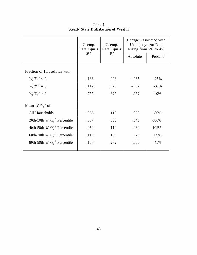
45

Table 1Steady State Distribution of Wealth

Unemp.Rate Equals

2%

Unemp.Rate Equals

4%

Change Associated withUnemployment Rate

Rising from 2% to 4%

Absolute Percent

Fraction of Households with:

W /Y < 0t t P .133 .098 -.035 -25%

W /Y = 0t t P .112 .075 -.037 -33%

W /Y > 0t t P .755 .827 .072 10%

Mean W /Y of:t t P

All Households .066 .119 .053 80%

20th-30th W /Y Percentilet t P .007 .055 .048 686%

40th-50th W /Y Percentilet t P .059 .119 .060 102%

60th-70th W /Y Percentilet t P .110 .186 .076 69%

80th-90th W /Y Percentilet t P .187 .272 .085 45%

46

Table 2Wealth Holdings for Households with Different Employment Histories

AllHouseholds

Unemployedin Year t

Unemployedin Year t-1

Unemployedin Year t-2

Not Unemp.in Last 3

Years

Fraction ofHouseholdswith:

W /Y < 0t t p .133 1.000 .975 .525 .041

W /Y = 0t t P .112 .000 .025 .275 .113

W /Y > 0t t P .755 .000 .000 .200 .840

Mean W / Yt tP .066 -.331 -.116 -.017 .095

Note: All calculations assume an unemployment rate of 2 percent.

47

Table 3SCF Summary Statistics

1983 1989 1992

Mean net worth $151,363 $143,393 $100,798

Median net worth $68,494 $67,545 $54,392

Net worth, 95th

percentile$590,320 $536,955 $360,119

Median ratio of networth to income

1.59 1.54 1.37

Percent with net worthof less than 1 month'sincome

8.0% 10.1% 9.1%

Percent with zero ornegative net worth

3.7% 5.3% 5.8%

Median net worth ofzero or negative networth households

-$1,338 -$1,450 -$2,475

Number of households 1689 1025 1032

Notes: Sample includes all households in SCF area with heads between the ages of 20 and 65who have been employed at the same job for at least three years. Sample excludes top andbottom 0.1 percentiles of wealth or income. All calculations were done on a weighted basis. Dollar amounts are expressed in 1992 dollars.

48

Table 4CPS First-Stage Estimation Resultsa

Dependent Variable = 1 if Unemployed in t+1; 0 Otherwise

1983 1989 1992

F-tests:b

Occupation 0.007 0.134 0.008

Industry 0.000 0.000 0.000

Region 0.012 0.000 0.000

Education 0.000 0.000 0.001

White 0.003 0.001 0.007

Female Head 0.051 0.105 0.011

Age 0.168 0.798 0.980

Age * Occupation 0.011 0.107 0.097

Age * Education 0.069 0.042 0.061

Mean Pr(û) 0.027 0.019 0.022

Std. Dev. Pr(û) 0.021 0.015 0.017

Number of Observations 59,252 60,026 63,351

Sample includes all individuals who were employed in t, including the self-employed.a

P-values.b

49

Table 5SCF First-Stage Estimation Results for Group Incomea

Dependent Variable = log(Y)

1983 1989 1992

F-tests:b

Occupation 0.684 0.361 0.847

Industry 0.009 0.111 0.084

Region 0.000 0.000 0.115

Education 0.417 0.742 0.016

White 0.667 0.061 0.463

Female Head 0.000 0.002 0.000

Home Owner 0.000 0.000 0.000

# Children 0.055 0.593 0.788

# Earners 0.000 0.000 0.000

Marital Status 0.000 0.008 0.058

Defined Benefit Coverage 0.000 0.000 0.009

Turned Down for Credit 0.331 0.076 0.897

Problems Servicing Debt 0.113 0.920 0.033

Age 0.000 0.000 0.016

Age * Occupation 0.008 0.059 0.759

Age * Education 0.376 0.553 0.248

Adjusted R2 0.46 0.41 0.28

Number of households 1688 1025 1032

Sample includes all individuals who were employed in t, including the self-employed.a

P-values.b

50

Table 6SCF Second-Stage Estimation Results

1983 1989 1992

Includingself-employed

Excludingself-employed

Includingself-employed

Excludingself-employed

Includingself-employed

Excludingself-employed

Pr(û) 0.52(0.50)

0.23(0.22)

-0.67(-0.28)

-1.03(-0.33)

0.03(0.01)

-0.60(-0.23)

ln Êp 0.09(1.24)

0.12(1.62)

0.23 (1.89)

0.44(2.44)

0.40(1.55)

0.26(1.58)

Number of Earners -0.04(-2.24)

-0.05(-2.58)

-0.08(-2.05)

-0.11(-1.94)

-0.18(-2.19)

-0.11(-1.99)

Owns Home 0.28 (9.00)

0.27(8.61)

0.32(5.80)

0.32(4.89)

0.28(3.46)

0.27(4.55)

Defined Benefit Pension -0.06(-3.43)

-0.04(-2.02)

-0.10(-2.60)

-0.08(-1.74)

-0.08(-1.39)

-0.02(-0.49)

Turned Down for Credit -0.05(-2.78)

-0.07(-3.15)

-0.03(-0.74)

-0.10(-2.14)

-0.06(-1.18)

-0.07(-1.72)

� 4.56 4.56 3.86 3.3 3.31 3.26

Overidentify restr. p-value 0.38 0.57 0.32 0.54 0.83 0.44

at median W/Êp 0.04(0.50)

0.01(0.22)

-0.05(-0.28)

-0.06(-0.32)

0.00(0.01)

-0.02(-0.23)

Number of Households 1689 1441 1025 835 1032 880

Note: Asymptotic t-statistics shown in parentheses. Regressions also include age, education, age*education,marital status, retirement status, race, sex, occupation, occupation*age, industry, and number of children.

51

Table 7SCF Second-Stage Estimation Results

1983 1989 1992

Includingself-employed

Excludingself-employed

Includingself-employed

Excludingself-employed

Includingself-employed

Excludingself-employed

Pr(û) -28.32(-2.53)

-26.75(-2.24)

-57.22(-1.99)

-66.09(-1.92)

-67.77(-1.99)

-50.46(-1.69)

Pr(û) * ln ÊP 2.96(2.58)

2.76(2.27)

5.72(1.98)

6.47(1.90)

6.85 (1.99)

5.05(1.68)

ln ÊP -0.03(-0.37)

0.01(0.12)

0.09(0.62)

0.25(1.17)

0.17(0.66)

0.11(0.57)

Ê percentile:P

10th 0.03(0.95)

0.03(0.51)

-0.01(-0.18)

-0.04(-0.60)

-0.01(-0.15)

-0.02(-.37)

30th 0.11(1.84)

0.04(1.34)

0.11(0.74)

0.06(0.30)

0.16(0.75)

0.03(0.38)

50th 0.29(2.14)

0.24(1.67)

0.27(1.18)

0.15(0.74)

0.17(1.17)

0.10(0.79)

70th 0.39(2.34)

0.33(1.87)

0.44(1.40)

0.24(1.03)

0.39(1.46)

0.14(1.05)

90th 0.52(2.47)

0.42(2.01)

0.71(1.61)

0.55(1.25)

0.77(1.67)

0.41(1.26)

Overidentify restr. p-value 0.50 0.71 0.32 0.61 0.89 0.46

Note: Asymptotic t-statistics shown in parentheses.

52

Table 8SCF Second-Stage Estimation Results: 1983, 1989, 1992 Pooled Data

Model without Pr(û) * ln ÊP

interactionModel with Pr(û) * ln ÊP

interaction

Includingself-employed

Excludingself-employed

Includingself-employed

Excludingself-employed

Pr(û) 0.95(1.34)

0.74(1.00)

-30.64(-3.34)

-27.15(-2.80)

Pr(û) * ln ÊP -- -- 3.15 (3.45)

2.77 (2.88)

ln ÊP 0.07 (1.85)

0.13(2.83)

0.00(0.04)

0.05(1.02)

Ê percentile:P

10th 0.02(1.34)

0.01(1.00)

0.01(0.64)

0.00(0.26)

30th 0.03(1.34)

0.02(1.00)

0.06(2.39)

0.05(1.76)

50th 0.06(1.34)

0.04(1.00)

0.17(3.07)

0.12(2.40)

70th 0.08(1.34)

0.05(1.00)

0.30(3.43)

0.21(2.75)

90th 0.09(1.34)

0.07(1.00)

0.43(3.62)

0.36(2.93)

Overidentify restr. p-value 0.31 0.59 0.34 0.57

Number of households 3746 3157 3746 3157

Note: Asymptotic t-statistics shown in parentheses.

53

Table 9Identification Issues: Alternative Excluded Controls

1983, 1989, 1992 Pooled Data

Instrument for ln Ê that is Excluded from ControlsP NoExcluded

InstrumentRegion Occupation Education Industry

Pr(û) -30.64(-3.34)

-20.15(-2.39)

-26.20(-2.81)

-28.58(-3.49)

-23.85(-2.82)

Pr(û) * ln ÊP 3.15(3.45)

1.95(2.33)

2.47(2.65)

2.95(3.67)

2.38(2.82)

ln ÊP 0.00(0.04)

-0.01(-0.25)

0.06(1.67)

-0.12(-2.86)

-0.09(-1.86)

Ê percentile:P

10th 0.01(0.64)

-0.02(-1.34)

-0.03(-2.69)

0.01(1.01)

-0.00(-0.40)

30th 0.06(2.39)

-0.00(-0.11)

-0.03(-1.02)

0.06(3.52)

0.03(1.01)

50th 0.17(3.07)

0.03(0.60)

-0.00(-0.06)

0.17(4.38)

0.09(1.64)

70th 0.30(3.43)

0.09(1.09)

0.05(0.59)

0.29(4.65)

0.17(2.05)

90th 0.43(3.62)

0.15(1.45)

0.13(1.09)

0.41(4.66)

0.26(2.33)

Overidentify restr. p-value 0.34 0.04 0.29 0.06 0.22

Exclusion p-value 0.01 0.00 0.00 0.00 n.a.

Note: Asymptotic t-statistics shown in parentheses.

54

Table 10Sensitivity Checks: 1983, 1989, 1992 Pooled Data

ReducedInstrumentsfor ln ÊP

Alternative Dependent Variables

Net FinancialAssets

NW excl.Real Estate

NW excl.Primary Res.

Pr(û) -25.37(-2.70)

0.14(0.10)

-6.98(-1.15)

-9.23(-1.53)

Pr(û) * ln ÊP 2.62(2.81)

-0.02(-0.15)

0.67 (1.11)

6.04(0.90)

ln ÊP 0.02(0.47)

0.01(1.65)

-0.00(-0.01)

0.01(0.18)

Ê percentile:P

10th 0.02(0.97)

-0.00(-0.63)

-0.01(-0.65)

-0.01(-0.79)

30th 0.09(2.39)

-0.00(-0.68)

-0.00(-0.07)

-0.00(-0.00)

50th 0.17(2.86)

-0.00(-0.64)

0.00(0.27)

0.01(0.44)

70th 0.30(3.05)

-0.00(-0.58)

0.01(0.49)

0.03(0.72)

90th 0.44(3.15)

-0.01(-0.51)

0.02(0.66)

0.06(0.94)

Overidentify restr. p-value 0.14 0.18 0.23 0.11

Region exclusion p-value 0.00 0.06 0.87 0.21

Note: Asymptotic t-statistics shown in parentheses.

-0.2 0.0 0.2 0.4 0.6w

0.2

0.4

0.6

0.8

1.0

CDF Figure 2

¬ Ρ = .04

Ρ = .02 ®

0.0 0.5 1.0 1.5 2.0 2.5x

0.2

0.4

0.6

0.8

1.0

1.2

1.4

c Figure 1

Ρ = .02 ®

¬ Ρ = .04

45 Degree