FEDERAL RESERVE BANK OF SAN FRANCISCO

WORKING PAPER SERIES

Currency Unions and Trade: A Post‐EMU Mea Culpa

Reuven Glick Federal Reserve Bank of San Francisco

Andrew K. Rose

University of California, Berkeley Haas School of Business

July 2015

Working Paper 2015-11

http://www.frbsf.org/economic-research/publications/working-papers/wp2015-11.pdf

Suggested citation:

Glick, Reuven, Andrew K. Rose. 2015. “Currency Unions and Trade: A Post‐EMU Mea Culpa.” Federal Reserve Bank of San Francisco Working Paper 2015-11. http://www.frbsf.org/economic-research/publications/working-papers/wp2015-11.pdf The views in this paper are solely the responsibility of the authors and should not be interpreted as reflecting the views of the Federal Reserve Bank of San Francisco or the Board of Governors of the Federal Reserve System.

Currency Unions and Trade: 

A Post‐EMU Mea Culpa Reuven Glick and Andrew K. Rose* 

 Revised Draft: July 17, 2015  

  

Abstract In our European Economic Review (2002) paper, we used pre‐1998 data on countries participating in and leaving currency unions to estimate the effect of currency unions on trade using (then‐) conventional gravity models.  In this paper, we use a variety of empirical gravity models to estimate the currency union effect on trade and exports, using recent data which includes the European Economic and Monetary Union (EMU).   We have three findings.  First, our assumption of symmetry between the effects of entering and leaving a currency union seems reasonable in the data but is uninteresting.  Second, EMU typically has a smaller trade effect than other currency unions; it has a mildly stimulating effect at best.  Third and most importantly, estimates of the currency union effect on trade are sensitive to the exact econometric methodology; the lack of consistent and robust evidence undermines confidence in our ability to reliably estimate the effect of currency union on trade.  Keywords: gravity, exports, trade, bilateral, common, fixed, time‐varying, country, specific, Poisson, currency union, monetary union, European  JEL Classification Numbers: F15, F33  Reuven Glick              Andrew K. Rose (correspondence) Federal Reserve Bank of San Francisco      Haas School of Business 101 Market St.,            University of California San Francisco CA 94105          Berkeley, CA USA 94720‐1900 Tel: (415) 974‐3184            Tel: (510) 642‐6609 Fax: (415) 974‐2168            Fax: (510) 642‐4700 E‐mail: reuven.glick@sf.frb.org        E‐mail: arose@haas.berkeley.edu  *  Glick is Group Vice President for International Research, Economic Research Department, Federal Reserve Bank of San Francisco.  Rose is Associate Dean for Academic Affairs and Chair of the Faculty, B.T. Rocca Jr. Professor, Haas School of Business at the University of California, Berkeley, NBER research associate, CEPR Research Fellow, and ABFER senior fellow.  We thank Genevieve Denoeux for research assistance, and Douglas Campbell, Thomas Chaney, José De Sousa, Zdenek Drabek, and workshop participants at the Monetary Authority of Singapore and the National University of Singapore.  The views expressed below do not represent those of the Federal Reserve Bank of San Francisco or the Board of Governors of the Federal Reserve System, or their staffs.  A current (PDF) version of this paper, the main STATA data sets used in the paper, and key output are available at http://faculty.haas.berkeley.edu/arose. 

1

1. Introduction 

In this paper we estimate the effect of currency unions on trade.  More specifically, we 

re‐estimate this effect using a variety of models and a panel of annual data that covers more 

than 200 countries between 1948 and 2013.  We do so largely to check the results of our 

European Economic Review (2002) paper, which used a panel approach to investigate the effect 

of currency unions on trade using data through 1997.  That work involved an assumption, a 

caveat, and some analysis.  In this paper, we examine each.   

Motivation: An Assumption, a Caveat, and a Finding 

In this paper, we use a data set that includes fifteen years of data for the Economic and 

Monetary Union in Europe, hereafter “EMU”.  We take advantage of this to ask three questions.  

First, we test whether our earlier assumption of symmetry between currency union entry and 

exit is justified in the data.  The data set of our EER (2002) paper included only 16 switches into 

but 130 switches out of currency unions before 1998.1  Given the paucity of data on entries into 

currency union, we explicitly assumed symmetry between entries and exits.2  We can now 

check this assumption, since the many entries into EMU give us a non‐trivial number of 

observations of currency union entries. 

Our second question is related: does EMU have a trade effect similar to that of other 

currency unions?  Our EER (2002) paper included no data on EMU, so we were cautious about 

the relevance of pre‐1998 data for EMU: 

“Caveats.  There are issues associated with the applicability of our results. Since our sample ends before EMU, most of the currency unions involved countries that were either small, poor, or both; our results may therefore be inapplicable to EMU.” 

 

2

Finally, we ask whether the (many) advances in empirical modeling of trade flows since 

our EER (2002) paper are materially relevant to estimating the currency union effect on trade.  

We worked hard in our earlier work to ensure that our results did not depend strongly on our 

precise methodology.  For instance we wrote (highlights added): 

 “To summarize: a number of different panel estimators all deliver the conclusion that currency union has a strong positive effect on trade.  … Our fixed effects estimates indicate that entry into/departure from a currency union leads bilateral trade to approximately double/halve, holding a host of other features constant.  This result is not only economically and statistically significant, but seems relatively robust...” 

“This result is economically large, statistically significant, and seems insensitive to a number of perturbations in our methodology.” 

 

The last dozen years has seen considerable methodological work in the area, perhaps most 

importantly the contributions of Anderson and van Wincoop (2003) and Santos Silva and 

Tenreyro (2006).  The literature has been ably surveyed recently by Head and Mayer (2014); see 

also Baldwin and Taglioni (2007).  We take advantage of this progress by estimating the effect 

of currency union on trade using newer techniques. 

To preview our conclusions, we find that: a) symmetry looks OK; b) EMU is way different 

from other currency unions; and most disturbingly c) econometric methodology matters a lot.  

Our finding of symmetry in trade patterns is weak and uninteresting, as we show below; it is 

also undermined by our final finding.  In the large, we find EMU has a mildly stimulating effect 

on trade at best.  Most importantly, we are forced to conclude that econometric methodology 

matters so much that it undermines confidence in our ability to estimate the effect of currency 

union on trade. 

 

3

2. Initial Methodology and Data Set 

  We are interested in estimating the effect of currency unions on aggregated 

international trade.  In our EER (2002) paper, we estimated a gravity model of international 

trade which was conventional for the time: 

ln(Tijt) = 0 + 1ln(YiYj)t + 2ln(YiYj/PopiPopj)t + 3lnDij + 4Langij + 5Contij + 6FTAijt   (1) 

+ 7Landlij + 8Islandij +9ln(AreaiAreaj) + 10ComColij + 11CurColijt   

+ 12Colonyij + 13ComNatij + CUijt + {δt} + ijt 

where i and j denote countries, t denotes time, and the variables are defined as: 

Tijt denotes the average nominal value of bilateral trade between i and j at time t, 

Y is real GDP, 

Pop is population, 

D is the distance between i and j, 

Lang is a binary variable which is unity if i and j have a common language, 

Cont is unity if i and j share a land border and 0 otherwise, 

FTA is unity if i and j belong to the same regional trade agreement and 0 otherwise, 

Landl is the number of landlocked countries in the country‐pair (0, 1, or 2). 

Island is the number of island nations in the pair (0, 1, or 2), 

Area is the land mass of the country, 

ComCol is unity if i and j were colonies after 1945 with the same colonizer  and 0 otherwise, 

CurCol is unity if i and j are colonies at time t and 0 otherwise, 

Colony is unity if i colonized j or vice versa and 0 otherwise, 

ComNat is unity if i and j remained part of the same nation during the sample (e.g., France 

and Guadeloupe, or the UK and Bermuda) and 0 otherwise, 

CU is unity if i and j use the same currency at time t and 0 otherwise, 

 is a vector of nuisance coefficients,  

4

{δ} is a mutually exclusive and jointly exhaustive set of year‐specific effects,  

ij represents the myriad other influences, assumed to be well behaved. 

We begin by re‐estimating this model on a longer data set that includes data through 

2013.  The coefficient of interest is γ, which we interpreted as the effect of a currency union on 

trade, ceteris paribus.  We follow our earlier work by estimating this model in two ways.3  First, 

we use ordinary least squares with standard errors which are robust to clustering (since dyads 

(country‐pairs) are likely to be highly dependent across years).  Second, we use the fixed effects 

“within” estimator by adding to (1) a comprehensive set of time‐invariant dyadic specific 

intercepts to the equation; this estimator thus exploits only the time series dimension of the 

data set around country‐pair averages.4 

The Data Set 

We rely on trade data drawn from the Direction of Trade (DOTS) data set assembled by 

the International Monetary Fund (IMF).  The DoT data set covers bilateral trade between over 

200 IMF country codes between 1948 and 2013 (with gaps; more on these below).   Not all of 

the areas covered are countries in the conventional sense of the word; colonies (e.g., Gibraltar), 

territories (e.g., Guam), overseas departments (e.g., Guadeloupe), countries that gained their 

independence during the sample (e.g., Guinea‐Bissau), and so forth are all included.  We use 

the term “country” simply for convenience.5  Bilateral trade on FOB exports and CIF imports is 

recorded in U.S. dollars.  We create an average value of bilateral trade between a pair of 

countries by averaging all of the four possible measures potentially available.6 

To this data set, we add a number of other variables that are necessary to estimate the 

gravity model.  We add population and real GDP data (in constant dollars) from three sources.  

5

Wherever possible, we use World Development Indicators (from the World Bank).  When the 

data are unavailable from the World Bank, we fill in missing observations with comparables 

from the Penn World Table Mark 7.1, and (when all else fails), from the IMF’s International 

Financial Statistics.  The series have been checked and corrected for errors.7 

We exploit the CIA’s World Factbook for a number of country‐specific variables.  These 

include: latitude and longitude, land area, landlocked and island status, physically contiguous 

neighbors, language, colonizers, and dates of independence.  We use these to create great‐

circle distance and other controls.  We obtain data from the World Trade Organization to create 

an indicator of regional trade agreements, and include: EEC/EC/EU; US‐Israel FTA; NAFTA; 

CARICOM; PATCRA; ANZCERTA; CACM, Mercosur, COMESA, and more.8 

Finally, we add information on whether the pair of countries was involved in a currency 

union.  By “currency union” we mean essentially that money was interchangeable between the 

two countries at a 1:1 par for an extended period of time, so that there was no need to convert 

prices when trading between a pair of countries; EMU is by far the most important 

contemporary example.  Hard fixes (such as those of Hong Kong or Denmark) do not qualify as 

currency unions under our definition.  We take our data from our earlier paper, which relied on 

the IMF’s Schedule of Par Values and issues of the IMF’s Annual Report on Exchange Rate 

Arrangements and Exchange Restrictions, supplemented with information from of The 

Statesman’s Yearbook, and extended through 2013 so that EMU is included.  Our definition of 

currency union is transitive; if dyads x‐y, and x‐z are in currency unions, then y‐z is a currency 

union.  In our sample, less than 2% of the observations involve dyads in a currency union.9 

 

6

3. Results with Older (Trade) Models 

We present estimates for (1) in Table 1.  For convenience and to provide a basis of 

comparison, we tabulate the estimates from our EER (2002) paper in the extreme left column.  

In our original paper, we estimated the key coefficient γ at 1.30, with a robust standard error of 

.13, implying that a pair of countries joined by a common currency trade over three times as 

much with each other (e1.3  3.7), holding other things constant.  As shown immediately to the 

right, our new data set – extended through 2013 with more than 200,000 extra observations – 

provides a point estimate of .92 with a (robust) standard error of .09.  While this is smaller, it is 

still statistically and economically substantive (e.92  2.51, with a t‐ratio exceeding 9).10 

By far the biggest recent event in monetary unions has been the establishment of the 

EMU.  In the next column of Table 1, we add a separate dummy for members of EMU, to 

dramatic effect.11  The currency union effect rises somewhat to 1.12, but the more interesting 

point estimate is that of EMU; the net effect of EMU membership is essentially nil in both 

economic and statistical terms; the net effect of EMU is (1.12‐1.10≈) .02 with a standard error 

of .08.  This is the first indication from the data that EMU seems to have a substantively 

different effect on trade than other monetary unions.12,13 

The essence of our 2002 paper was to take maximal advantage of currency union status 

using a panel estimator with fixed dyadic (country‐pair) effects, rather than relying simply on 

the least squares results of Table 1.  Accordingly, we add (more than 14,000) dyadic fixed 

effects and re‐estimate (1); our (within) results are presented in Table 2.  As in Table 1, we 

tabulate results from our earlier paper at the extreme left. 

7

The estimates in Table 2 indicate that γ has changed little with data revisions and 

extensions, from .65 to .63.14  However, when we add a separate dummy for EMU, the gross 

currency union estimate rises to .75, while the additional effect of EMU is significantly negative 

in both economic and statistical terms, as in Table 1.  The net effect of EMU on trade is now 

large and positive; the point estimate is (.75‐.33≈) .41 with a standard error of .05, implying that 

EMU entry expands trade by (e.41‐1≈) 51%.  Clearly the post‐1997 data changes our view of the 

currency union effect on trade substantively; even with the same statistical models, the data is 

delivering different results because of EMU. 

The impression of a post‐1997 break in the effect is reinforced by the Chow tests 

tabulated in Table 3.  The top row tests the hypothesis of model constancy – identical slopes of 

γ and {β} – when one compares the post‐1997 period with the entire sample.  The null 

hypothesis of model constancy is grossly inconsistent with the results of both the least squares 

estimator of Table 1 and the fixed effects estimator of Table 2.  The bottom row of Table 3 also 

finds non‐constancy for a narrower hypothesis; EMU observations need to be modeled 

differently from other observations. 

Symmetry 

The results in Tables 1 and 2 are attempts to estimate the steady state effect of 

currency union on trade, holding other things constant.  A related question is whether the trade 

effects of currency union entry and effect are symmetric; another question of interest is how 

long these effects take to make themselves apparent.  In our earlier paper, we had a large 

number of observations on exits from currency unions but only a small number of entries into 

currency unions; hence we were forced to make our assumption of symmetry between the 

8

dynamic trade effects of currency union exit and entry.  Since EMU began in 1999, we now have 

fifteen years of EMU data and can use this to test our assumption of symmetric dynamics.  We 

begin with a graphical approach. 

We replace our simple currency union dummy in (1) with lags after both currency union 

exits and entries and re‐estimate our equation; we then use these results to test the hypothesis 

of equality between the dynamic trade effects after currency union exit with the (opposite 

signed) effects after entry.  We use fourteen lags, since we have that many years of data 

following the start year of EMU.  We also add a comparable number of leads (before both 

currency union exit and entry) so as to be able to test for symmetry in the run‐up to monetary 

union exit/entry.  That is, we estimate: 

 

ln(Tijt) = 0 + 1ln(YiYj)t + 2ln(YiYj/PopiPopj)t + 3lnDij + 4Langij + 5Contij + 6FTAijt   (1’) 

+ 7Landlij + 8Islandij +9ln(AreaiAreaj) + 10ComColij + 11CurColijt   

+ 12Colonyij + 13ComNatij + ΣkθkENTRYijt‐k + ΣkφkEXITijt‐k + {δt} + ijt 

 

where ENTRYijt‐k is a dummy which is 1 if countries i and j entered a currency union at time t‐k 

and 0 otherwise; EXIT is defined analogously for exits from current union; and we let k run from 

‐14 to 14. 

The least squares point estimates of {φ} are portrayed in the upper‐left graph of Figure 

1, along with the corresponding +/‐ two standard error band; the lower‐left graph presents 

estimates of {θ}.  We are interested in checking the comparability between EMU and other 

currency unions.  Accordingly, we divide the ENTRY dummies into two mutually and jointly 

9

exhaustive sets of dummies and graph the resulting coefficients on the right side of the figure.  

Analogues estimated with dyadic fixed effects are in Figure 2; since we have more confidence in 

the latter, we focus on them.15 

Most of the results in Figure 2 seem intuitive.  The effect of currency union on trade is 

substantial, in both economic and statistical terms, before currency union exit.  Upon exit, the 

effect starts to shrink in both economic and statistical terms, though it lingers on even fourteen 

years after exit.  The effect after currency union entry is also striking; there seems to be a 

positive effect before entry, perhaps indicating that the event is endogenous (a different issue).  

The statistical effect of currency union entry on trade seems substantial, even long after entry.   

Estimates of (1’) allow us to test for symmetry rigorously.  We are particularly interested 

in symmetry between the (dynamic) effects of entry into and exit from currency union.  We ask 

“Does the additional boost to trade after currency union entry k years ago equal the reduction 

in trade after currency union exit k years ago?”16  Since we estimate both leads and lags before 

entry/exit, we can test for symmetry both before and after currency entry/exit, as well as both 

before and after simultaneously.  Our F‐tests are tabulated in Table 4; the different columns 

present results from our least squares and fixed effects estimators. 

The hypothesis of symmetric trade effects of currency union entry/exit works 

reasonably well for the fixed effect estimator, as indicated by the low F‐tests.  The same is true 

when we end the sample in 1997, in the middle of Table 4.  The only serious sign of asymmetry 

is the period before currency union entry/exit in the truncated (pre‐1998) sample.  For both 

samples of data, the least squares estimates are less consistent with symmetry.  At the bottom 

of the table, we present results which compare EMU with other currency unions.  EMU 

10

observations seem to have trade effects which are similar to other currency unions, especially 

after entry.  It is especially striking to us that the FE estimates are consistent with the 

hypothesis that the trade effect after EMU entry is symmetric to that after exit from other 

currency unions; this seems close to validating our original assumption of symmetry.  With new 

data and old methodology, the essence of our earlier work still looks reasonable; the question 

is whether it stands up to greater econometric scrutiny.  We now turn to that question. 

 

4. Results with Newer (Export) Models 

  We now pursue “theory‐consistent estimation” of the gravity equation, closely following 

the suggestions in the recent survey by Head and Mayer (2014).  We focus on their “LSDV” 

(Least Squares with time‐varying country Dummy Variables) technique which they show works 

well in many situations.  In particular, we estimate: 

 

ln(Xijt) = CUijt + 3lnDij + 4Langij + 5Contij + 6FTAijt + 10ComColij + 11CurColijt      (2) 

+ 12Colonyij + 13ComNatij + {λit} + {ψjt} + ijt 

 

where: 

Xijt denotes the nominal value of bilateral exports from i to j at time t, 

{λit} is a complete set of time‐varying exporter dummy variables, and 

{ψjt} is a complete set of time‐varying importer dummy variables. 

 

11

This equation is closely related to (1), with two substantive differences.  First, the equation 

estimates the effect of currency union on (log) exports rather than trade.  Second, it holds 

constant all country‐specific “monadic” phenomena (both time‐invariant, such as land area, and 

time‐varying, such as GDP) rather than time‐invariant dyadic phenomena.  Consistently, (2) can 

only estimate the effect of pair‐specific phenomena, like the currency union effect on exports. 

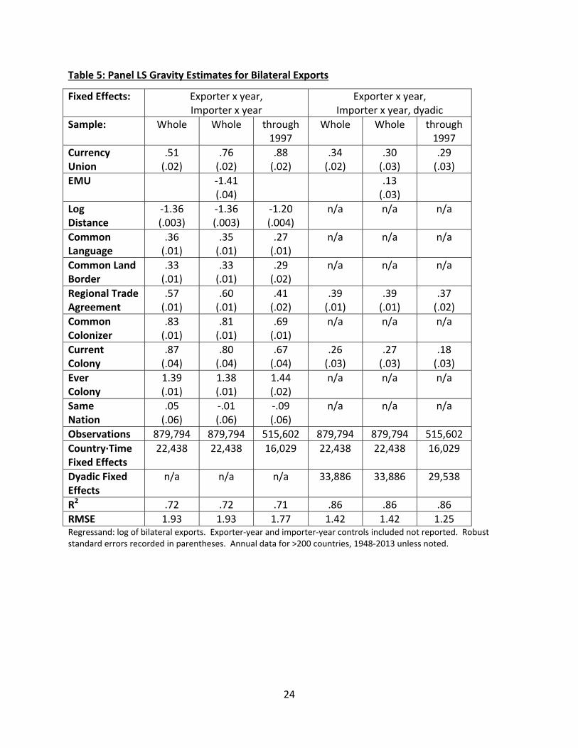
  The estimate of γ presented at the extreme left column of Table 5 is economically and 

statistically significant.  Roughly comparable to the .63 point trade effect of Table 2, the point 

estimate of the currency union effect on exports is .51.  This is a large effect in economic (e.51 ‐1 

≈ 67%) and statistical terms (the t‐ratio exceeds 20).  Point estimates for the other bilateral 

estimates also seem intuitive in sign and size.  We note in passing that even stronger results 

characterize the sample restricted to data before 1998, as shown in the right‐hand column.17 

  The analysis presented above suggests that EMU has a substantially smaller trade effect 

than other currency unions.  We check by adding a separate EMU dummy variable to our export 

model of (2); the estimates are also presented in Table 5.  Consistent with our earlier results 

but even more dramatically, the export‐stimulating effect of EMU is lower than other currency 

unions.  While other currency unions now seem to raise exports significantly (e.76 ‐1 ≈ 114%, 

with a t‐ratio of 38), EMU more than completely offsets this effect.  Indeed, the net effect of 

EMU on exports is negative; the point estimate is (.76‐1.41≈) ‐.65 with a standard error of .03. 

Baldwin and Taglioni (2007) recommend adding dyadic fixed effects to (2), precisely in 

the context of estimating the currency union effect on exports.18  We follow their suggestion on 

the right‐hand side of Table 5.  Adding country‐pair fixed effects (to the time‐varying 

exporter/importer effects) reduces the currency union effect, though it remains positive and 

12

significant.  However, the extra marginal effect of EMU is now positive; EMU is now estimated 

to raise exports by an economically significant (exp(.43)‐1≈) 54%, an effect significantly 

different from zero at any confidence level (the t‐ratio exceeds 20).  The dyadic effects add 

considerable explanatory power to the exports equation while reversing the EMU effect; a 

confusing state of affairs, to say the least. 

Symmetry 

  We are interested in whether the effects of currency union exit are symmetric with 

those of currency union entry; we are also interested in whether currency unions are all alike, 

or whether EMU is different.  Much as we did above in (1’), we re‐estimate our model after 

adding dynamic effects to our panel regression for exports: 

 

ln(Xijt) = CUijt + 3lnDij + 4Langij + 5Contij + 6FTAijt + 10ComColij + 11CurColijt      (2’) 

+ 12Colonyij + 13ComNatij + ΣkθkENTRYijt‐k + ΣkφkEXITijt‐k + {λit} + {ψjt} + ijt 

 

Figure 3 is analogous to Figures 1 and 2, but portrays least squares point estimates of 

{φ} (in the top‐left) and {θ} (in the lower‐left) for exports, along with corresponding +/‐ two 

standard error bands.  As before, we also divide the ENTRY dummies into two mutually and 

jointly exhaustive sets of dummies for EMU and non‐EMU unions, and graph the resulting 

coefficients on the right side of the figure. 

The results of Figure 3 are difficult to interpret, at least in any straightforward way.  In 

our sample, we have 1484 (bilateral) observations when an exporter‐importer dyad severed a 

13

currency union.  This seems like a large sample of observations, even taking into account 

dependencies between them.  Yet leaving a currency union seems to have little effect on 

exports.  More bizarrely, currency union entry has little effect on exports and seems indeed to 

lead them to decline significantly after some time.  The graphs on the right show that this 

finding stems from EMU, the source of many observations of monetary union entry.  Interesting 

enough, the effects of currency union entry and exit seem equally, and symmetrically, bizarre.  

This finding of symmetry is ratified by the formal statistical tests tabulated in Table 6; these are 

analogous to those of Table 4.  The low F‐tests are consistent with the hypothesis that the 

dynamic export effect of currency union entry is equal to (minus) that of currency union exit, 

both before and after currency union exit/entry.  We take this as cold comfort, since it is the 

result of both exit and entry effects being equally weird, not exactly a ratification of the 

assumption we made in our (2002) EER paper based on sensible results. 

On the other hand, adding dyadic fixed effects changes things radically.  This is 

demonstrated in Figure 4, which is the analogue to Figure 3 after country‐pair fixed effects are 

added to (2’).  The results are intuitive and echo those of Figure 2; exit from a currency union 

seems to make exports fall after a lag.  More importantly, currency union entry – especially into 

EMU – leads exports to rise significantly over time. 

Handling Zeros and Heteroskedasticity 

What is the source of the inconsistent and sometimes bizarre effects that currency 

union (especially EMU) entry seems to have on exports?  It may be the result of a short span of 

data on EMU; we only have fifteen years of data on EMU now, while we exploited 30 lags in our 

14

(2002) EER paper.  Still, the literature has recently focused on more technical problems likely to 

render the estimates from (2) and (2’) problematic. 

Santos Silva and Tenreyro (2006) argued persuasively that least squares estimates of (1) 

and (2) are likely to result in biased estimates of true gravity effects because of 

heteroskedasticity and/or the presence of numerous discarded observations of zero trade; 

Head and Mayer (2014) provide a summary of the associated issues.  Zero trade observations 

can arise because of rounding errors, missing observations, or truly zero trade; their presence is 

certainly endemic in our data set.19  To handle this problem, Santos Silva and Tenreyro (2006) 

propose Poisson pseudo‐maximum‐likelihood (hereafter “Poisson”) estimation.  Poisson, least 

squares, and a number of alternative estimators are studied further by Head and Mayer (2014); 

below, we follow their suggestion to compare Poisson and least squares.  In particular, we 

estimate annual cross‐sections with least squares: 

 

ln(Xijt) = CUijt + EMUEMUijt + 3lnDij + 4Langij + 5Contij + 6FTAijt + {λit} + {ψjt} + ijt   (3) 

 

for years t=1960, …, 2013.20  We then compare the estimates of γ with those from comparable 

annual cross‐sections estimated by Poisson of: 

 

Xijt = CUijt + EMUEMUijt + 3Dij + 4Langij + 5Contij + 6FTAijt + {λit} + {ψjt} + ijt     (3’) 

 

where Xijt=0 if we have zero or missing exports for the relevant countries.21 

15

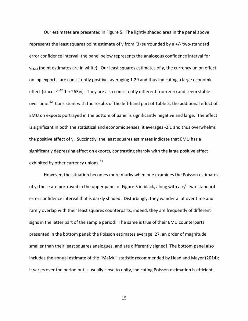
Our estimates are presented in Figure 5.  The lightly shaded area in the panel above 

represents the least squares point estimate of γ from (3) surrounded by a +/‐ two‐standard 

error confidence interval; the panel below represents the analogous confidence interval for 

γEMU (point estimates are in white).  Our least squares estimates of γ, the currency union effect 

on log exports, are consistently positive, averaging 1.29 and thus indicating a large economic 

effect (since e1.29‐1 ≈ 263%).  They are also consistently different from zero and seem stable 

over time.22  Consistent with the results of the left‐hand part of Table 5, the additional effect of 

EMU on exports portrayed in the bottom of panel is significantly negative and large.  The effect 

is significant in both the statistical and economic senses; it averages ‐2.1 and thus overwhelms 

the positive effect of γ.  Succinctly, the least squares estimates indicate that EMU has a 

significantly depressing effect on exports, contrasting sharply with the large positive effect 

exhibited by other currency unions.23 

However, the situation becomes more murky when one examines the Poisson estimates 

of γ; these are portrayed in the upper panel of Figure 5 in black, along with a +/‐ two‐standard 

error confidence interval that is darkly shaded.  Disturbingly, they wander a lot over time and 

rarely overlap with their least squares counterparts; indeed, they are frequently of different 

signs in the latter part of the sample period!  The same is true of their EMU counterparts 

presented in the bottom panel; the Poisson estimates average .27, an order of magnitude 

smaller than their least squares analogues, and are differently signed!  The bottom panel also 

includes the annual estimate of the “MaMu” statistic recommended by Head and Mayer (2014); 

it varies over the period but is usually close to unity, indicating Poisson estimation is efficient. 

16

To summarize, our least squares panel results with time‐varying country fixed effects 

but without dyadic effects indicate that EMU has a significantly dampening effect on exports 

which more than overwhelms the positive effect of other currency unions.  On the other hand, 

adding dyadic effects reverses this conclusion altogether.  More worrying still perhaps is the 

divergence between Poisson and LS cross‐sectional estimates of the effects of both currency 

unions and EMU on exports.  All this means that we have little confidence in our estimates.  Our 

least squares estimates of the effect of currency union on exports (without dyadic effects) are 

positive, reasonably stable and both economically and statistically significant; the Poisson 

estimates vary a lot over time and are often negative.  Where our LS estimates of the EMU 

effect on exports are large and negative, our Poisson estimates are small and positive.  The fact 

that the precise econometric methodology matters a lot is a strong and disturbing result of our 

analysis that undermines any positive findings. 

Summarizing the Net EMU Effect 

  The most interesting and important coefficient of interest in this literature is the net 

effect of EMU on trade and exports, ceteris paribus; Table 7 summarizes the  estimates 

together with some robustness checks.  We present results for the five different estimation 

techniques we have used (pooled OLS on trade, dyadic FE on trade, time‐varying 

exporter/importer FE on exports, dyadic and time‐varying exporter/importer FE on exports, and 

cross‐sectional Poisson on exports).  For the four different panel estimators, we present five 

robustness checks as well as our default estimates: a) sampling data every five years (instead of 

annually); b) only retaining dyads for similarly‐sized countries (those with GDPs that differ by 

less than a factor of five); c) only retaining dyads where bilateral trade is a small fraction (less 

17

than 10%) of total trade for both countries; d) dropping post‐2006 observations; and e) 

dropping observations where the residual is greater than two standard deviations from zero.24 

  After fifteen years, what do the data indicate that the effect of EMU has been on 

international trade?  The signal is hard to find in the noise.  Pooled least squares estimates of 

(1) imply that the trade effect has been insignificantly different from zero in both the economic 

and statistical senses.  Further, this result is insensitive across the five sensitivity tests.  But 

adding dyadic fixed effects leads one to conclude that EMU has significantly raised trade, and 

again this result seems robust.  Moving to a more recent model of exports with time‐varying 

country fixed effects, (2), leads to the conclusion that EMU has significantly reduced trade, and 

once more this conclusion seems insensitive.  Still, adding dyadic fixed effects reverses the 

result and restores the conclusion of a large positive effect of EMU on exports, another robust 

result.  But Poisson estimation seems reasonable, given the missing observations, MaMu test 

results, and heteroskedasticity in the data.  Of the fifteen (annual) Poisson estimates of the net 

EMU effect, four are negative and insignificant, five are positive and insignificant and the final 

five are positive, statistically significant and economically non‐trivial.  Since the estimators are 

basically presented in increasing order of plausibility and scientific respectability, one could 

conclude that EMU seems to have at least a mildly stimulating effect on exports.  If forced to 

make a quantitative assessment, that’s what we would conclude.  However, the switches and 

reversals across methodologies make us nervous of any bold statements. 

 

 

18

5. Summary and Conclusion 

In our EER (2002) paper, we concluded that “a pair of countries which joined/left a 

currency union experienced a near‐doubling/halving of bilateral trade.”  This conclusion was 

based on: a) an assumption of symmetry between the consequences of currency union exits 

and entries; b) a caveat that EMU might be different from other currency unions; and c) 

evidence that our results were insensitive to the precise econometric methodology.  In this 

paper, we re‐estimate this effect using a variety of models and a panel of annual data that 

covers more than 200 countries between 1948 and 2013, including fifteen years of EMU.  As it 

turns out, the assumption of symmetry between entry and exit seems reasonable, if often 

uninteresting.  The fear that prompted our caveat was warranted; EMU seems to be different 

from other currency unions.  Importantly, we have little confidence in either of our first two 

results because of our final finding.  We were wrong on the final point of our EER (2002) paper; 

the econometric methodology used to estimate the currency union effect matters, a lot. 

If one took seriously the results from least squares estimation without fixed effects, one 

would conclude that EMU had essentially no effect on trade, while other currency unions had 

an economically and statistically huge effect.  Moreover, this result seems insensitive to a 

variety of perturbations of the basic methodology.  On the other hand, adding dyadic fixed 

effects substantially lowers one’s estimate of the currency union effect, while simultaneously 

and significantly raising the effect of EMU; again, these results seem robust in the context of 

the technique.  But switching to a more modern model of exports with time‐varying country 

fixed effects would again change the conclusion, since those estimates imply that EMU has an 

enormous negative effect on exports while other currency unions have a huge positive effect; 

19

sadly, these results also seem insensitive within technique.  Then again, adding dyadic fixed 

effects to this model lowers the currency union effect but leaves it positive and significant, 

while indicating that EMU has an even larger positive effect on exports.  Finally, Poisson 

estimates of the currency union on exports vary substantially over time and rarely overlap with 

those of least squares; they are often small, negative and insignificantly different from zero.  

We conclude that it is currently beyond our ability to estimate the effect of currency 

unions on aggregate trade with much confidence.   

20

References  Anderson, James E. and Eric Van Wincoop. (2003) “Gravity and Gravitas: A Solution to the Border Puzzle” American Economic Review 93(1), 170‐192.  Baldwin, Richard (2006). “The Euro’s Trade Effects” ECB Working Paper Series No. 594.  Baldwin, Richard and Daria Taglioni (2007). “Trade Effects of the Euro” Journal of Economic Integration 22(4), 780‐818.  Baldwin, Richard, Virginia DiNino, Lionel Fontagné, Robert De Santis, and Daria Taglioni (2008), “Study on the Impact of the Euro on Trade and Foreign Direct Investment” European Economy Economic Papers 321.  De Sousa, José (2012). “The Currency Union Effect on Trade is Decreasing over Time” Economics Letters 117, 917‐920.  Frankel, Jeffrey (2010). “The Estimated Trade Effects of the Euro” chapter 5 in Alesina, A. and F.  Giavazzi (eds), Europe and the Euro (University of Chicago Press, Chicago), 169‐212.  Glick, Reuven and Andrew K. Rose (2002). “Does a Currency Union Affect Trade? The Time‐Series Evidence” European Economic Review 46(6), 1125‐51.  Head, Keith and Thierry Mayer (2014). “Gravity Equations: Workhorse, Toolkit, and Cookbook” chapter 3 in Gopinath, G., E. Helpman and K. Rogoff (eds), vol. 4 of the Handbook of International Economics (Elsevier, Amsterdam), 131–95.  Santos Silva, J.M.C., and Silvana Tenreyro (2006). “The Log of Gravity” Review of Economics and Statistics 88(4), 641‐658. 

21

Table 1: Pooled Panel Least Squares Gravity Estimates for Bilateral Trade 

  EER 2002  New  with EMU dummy 

through 1997 

Currency  Union 

1.30 (.13) 

.92 (.09) 

1.12 (.11) 

1.09 (.11) 

EMU        ‐1.10 (.13) 

 

Log Distance 

‐1.11 (.02) 

‐1.06 (.02) 

‐1.06 (.02) 

‐.94 (.02) 

Log Product Real GDPs 

.93 (.01) 

1.03 (.01) 

1.03 (.01) 

.96 (.01) 

Log Product Real GDP/capita 

.46 (.02) 

.11 (.01) 

.11 (.01) 

.13 (.01) 

Common Language 

.32 (.04) 

.54 (.04) 

.53 (.04) 

.42 (.04) 

Common Land Border 

.43 (.12) 

.71 (.11) 

.71 (.11) 

.63 (.11) 

Regional Trade Agreement 

.99 (.13) 

.89 (.04) 

.92 (.04) 

.95 (.07) 

Number Landlocked 

‐.14 (.03) 

‐.38 (.03) 

‐.38 (.03) 

‐.18 (.03) 

Number  Islands 

.05 (.04) 

.19 (.03) 

.19 (.03) 

.11 (.04) 

Log Product  Land Areas 

‐.09 (.01) 

‐.06 (.01) 

‐.06 (.01) 

‐.07 (.01) 

Common Colonizer 

.45 (.07) 

.60 (.06) 

.58 (.06) 

.50 (.07) 

Current  Colony 

.82 (.25) 

1.02 (.22) 

.95 (.22) 

.86 (.23) 

Ever  Colony 

1.31 (.13) 

1.19 (.13) 

1.18 (.13) 

1.31 (.14) 

Same  Nation 

‐.23 (1.05) 

‐1.18 (.21) 

‐1.16 (.21) 

‐1.14 (.21) 

Observations  219,558  426,953  426,953  238,995 

R2  .64  .67  .67  .64 

RMSE  2.02  2.03  2.03  1.92 

Years  1948‐1997  1948‐2013  1948‐2013  1948‐1997 Regressand: log of bilateral trade.  Intercept and year controls not reported.  Standard errors robust to dyadic clustering recorded in parentheses.  Annual data for >200 countries. 

22

Table 2: Dyadic Fixed Effects Gravity Estimates for Bilateral Trade 

  EER 2002   New   with EMU dummy 

through 1997 

Currency Union  .65 (.05) 

.63 (.07) 

.75 (.10) 

.68 (.10) 

EMU      ‐.33 (.11) 

 

Log Product  Real GDPs 

.05 (.01) 

.69 (.04) 

.69 (.04) 

.41 (.05) 

Log Product  Real GDP/capita 

.79 (.01) 

.42 (.04) 

.42 (.04) 

.65 (.05) 

R2: Within  .12  .20  .20  .14 

Years  1948‐1997  1948‐2013  1948‐2013  1948‐1997 

Observations  219,558  426,953  426,953  238,995 

Country‐Pair Fixed Effects 

11,178  14,801  14,801  13,342 

Regressand: log of bilateral trade.   Fixed dyadic (pair‐specific) effects and year effects included but not reported.  Other controls not reported: a) regional FTA membership, b) current colony.  Robust standard errors in parentheses.  Annual data for >200 countries. 

  

Table 3: Chow Tests for Bilateral Trade 

  Least Squares  Dyadic FE 

Post‐1997 versus all  89. (.00) 

134. (.00) 

EMU versus all  27. (.00) 

10. (.00) 

F‐tests (P‐values reported parenthetically) for hypothesis of identical slopes, using regression models from previous tables. 

    

23

Table 4: Symmetry Tests for Bilateral Trade 

  Fixed Effects:  Time  Dyadic, Time 

Whole Sample 

After CU Entry =  ‐ After CU Exit? 

2.8 (.00) 

1.4 (.15) 

Before CU Entry =  ‐ Before CU Exit? 

1.4 (.13) 

1.8 (.04) 

Both  2.6 (.00) 

1.8 (.01) 

1948‐1997  After CU Entry =  ‐ After CU Exit? 

1.4 (.13) 

1.1 (.35) 

Before CU Entry =  ‐ Before CU Exit? 

1.5 (.12) 

2.3 (.00) 

Both  2.2 (.00) 

2.0 (.00) 

Whole Sample 

After non‐EMU CU Entry =  After EMU Entry? 

1.6 (.09) 

.8 (.73) 

Before non‐EMU CU Entry = Before EMU Entry? 

1.1 (.39) 

1.3 (.17) 

Both  1.4 (.07) 

1.4 (.07) 

After non‐EMU CU Exit =  ‐ After EMU Entry? 

2.1 (.01) 

1.1 (.36) 

F‐tests with P‐values reported parenthetically, calculated from regressions of log of bilateral trade.  Regressors included: 14 leads, 14 lags and contemporaneous values of both currency union entry and currency union exit; log distance; log product real GDP; log product real GDP per capita; common language; common land border; regional FTA membership, # landlocked; # islands; log product area; common colonizer; current colony/colonizer; ever colony/colonizer; common country. Intercept and year controls not reported.  Annual data for >200 countries, 1948‐2013 unless noted. 

 

   

24

Table 5: Panel LS Gravity Estimates for Bilateral Exports 

Fixed Effects:  Exporter x year,  Importer x year 

Exporter x year,  Importer x year, dyadic 

Sample:  Whole  Whole  through 1997 

Whole  Whole  through 1997 

Currency Union 

.51 (.02) 

.76 (.02) 

.88 (.02) 

.34 (.02) 

.30 (.03) 

.29 (.03) 

EMU    ‐1.41 (.04) 

    .13 (.03) 

 

Log Distance 

‐1.36 (.003) 

‐1.36 (.003) 

‐1.20 (.004) 

n/a  n/a  n/a 

Common Language 

.36 (.01) 

.35 (.01) 

.27 (.01) 

n/a  n/a  n/a 

Common Land Border 

.33 (.01) 

.33 (.01) 

.29 (.02) 

n/a  n/a  n/a 

Regional Trade Agreement 

.57 (.01) 

.60 (.01) 

.41 (.02) 

.39 (.01) 

.39 (.01) 

.37 (.02) 

Common Colonizer 

.83 (.01) 

.81 (.01) 

.69 (.01) 

n/a  n/a  n/a 

Current Colony 

.87 (.04) 

.80 (.04) 

.67 (.04) 

.26 (.03) 

.27 (.03) 

.18 (.03) 

Ever Colony 

1.39 (.01) 

1.38 (.01) 

1.44 (.02) 

n/a  n/a  n/a 

Same Nation 

.05 (.06) 

‐.01 (.06) 

‐.09 (.06) 

n/a  n/a  n/a 

Observations  879,794  879,794  515,602  879,794  879,794  515,602 

Country∙Time Fixed Effects 

22,438  22,438  16,029  22,438  22,438  16,029 

Dyadic Fixed Effects 

n/a  n/a  n/a  33,886  33,886  29,538 

R2  .72  .72  .71  .86  .86  .86 

RMSE  1.93  1.93  1.77  1.42  1.42  1.25 Regressand: log of bilateral exports.  Exporter‐year and importer‐year controls included not reported.  Robust standard errors recorded in parentheses.  Annual data for >200 countries, 1948‐2013 unless noted. 

   

25

Table 6: Symmetry Tests for Bilateral Exports 

    Exporter x year, Importer x year FE 

Dyadic, Exporter x year, Importer x year FE 

Whole Sample 

After CU Entry =  ‐ After CU Exit? 

1.4 (.15) 

.8 (.71) 

Before CU Entry =  ‐ Before CU Exit? 

.4 (.98) 

.8 (.68) 

Both  1.0 (.41) 

1.0 (.49) 

1948‐1997 

After CU Entry =  ‐ After CU Exit? 

.6 (.90) 

1.2 (.30) 

Before CU Entry =  ‐ Before CU Exit? 

1.0 (.44) 

1.0 (.45) 

Both  .8 (.73) 

1.2 (.21) 

Whole Sample 

After non‐EMU CU Entry = After EMU Entry? 

1.8 (.04) 

1.3 (.17) 

Before non‐EMU CU Entry = Before EMU Entry? 

.6 (.89) 

1.4 (.16) 

Both  1.2 (.27) 

2.8 (.00) 

After non‐EMU CU Exit =    ‐ After EMU Entry? 

5.4 (.00) 

.9 (.51) 

F‐tests with P‐values reported parenthetically, calculated from regressions of log of bilateral exports.  Regressors included: 14 leads, 14 lags and contemporaneous values of both currency union entry and currency union exit; log distance; common language; common land border; regional FTA membership, common colonizer; current colony/colonizer; ever colony/colonizer; common country. Intercept and year controls not recorded.  Annual data for >200 countries. 

 

   

26

Table 7: Net EMU Effect 

Regressand  Log Trade  Log Exports 

Fixed Effects  Time  Time, Dyadic (country‐pair) 

Exporter x Time, Importer x Time 

Exporter x Time, Importer x Time, 

Dyadic 

Default  .02 (.08) 

.41(.05) 

‐.65(.03) 

.43 (.02) 

Data at Five‐Year Intervals 

.03 (.08) 

.34(.06) 

‐.50(.07) 

.51 (.05) 

Similarly‐sized Countries 

.08 (.11) 

.28(.08) 

‐.72(.04) 

.42 (.03) 

No Important Trade Relation 

.21 (.09) 

.36(.06) 

‐.27(.04) 

.51 (.03) 

Drop post‐2006 

‐.02 (.10) 

.46(.06) 

‐1.12(.05) 

.19 (.03) 

Drop >|2σ| Residuals 

‐.05 (.07) 

.42(.05) 

‐.64(.03) 

.30 (.02) 

 

Poisson 1999  ‐.14 

(.08) 

2000  ‐.10 (.08) 

2007  .12 (.08) 

2001  ‐.10 (.08) 

2008  .13 (.08) 

2002  ‐.11 (.08) 

2009  .21 (.08) 

2003  .00 (.08) 

2010  .26 (.09) 

2004  .07 (.08) 

2011  .30 (.09) 

2005  .08 (.08) 

2012  .29 (.10) 

2006  .10 (.08) 

2013  .31 (.10) 

 The coefficients tabulated denote the net EMU effect, i.e., the sum of coefficients on (CU+EMU) dummy variables; robust standard errors recorded in parentheses.  Least squares estimation.  Regressors included but not reported for trade models: non‐EMU currency union dummy; log distance; log product real GDP; log product real GDP per capita; common language; common land border; regional FTA membership; # landlocked; # islands; log product area; common colonizer; current colony/colonizer; ever colony/colonizer; common country; year controls.  Regressors included but not recorded for export models: non‐EMU currency union dummy; log distance; common language; common land border; regional FTA membership; common colonizer; current colony/colonizer; ever colony/colonizer; common country; intercept.  Regressors included but not recorded for Poisson models: non‐EMU currency union dummy; distance; common language; common land border; regional FTA membership.  Annual data for >200 countries, 1948‐2013 unless otherwise marked.   

27

Figure 1 

-1.5

-.5

.51.

5

-15 -10 -5 0 5 10 15Years from Exit

742 Exits

-1.5

-.5

.51.

5

-15 -10 -5 0 5 10 15Years from Entry

161 non-EMU Entries

-1.5

-.5

.51.

5

-15 -10 -5 0 5 10 15Years from Entry

392 Entries

-1.5

-.5

.51.

5

-15 -10 -5 0 5 10 15Years from Entry

231 EMU Entries

LS Gravity coefficients, with +/- 2 standard error bandEffects of Currency Union Transitions on log Trade

28

Figure 2 

-1.5

-.5

.51.

5

-15 -10 -5 0 5 10 15Years from Exit

742 Exits

-1.5

-.5

.51.

5

-15 -10 -5 0 5 10 15Years from Entry

161 non-EMU Entries

-1.5

-.5

.51.

5

-15 -10 -5 0 5 10 15Years from Entry

392 Entries

-1.5

-.5

.51.

5

-15 -10 -5 0 5 10 15Years from Entry

231 EMU Entries

FE Gravity coefficients, with +/- 2 standard error bandEffects of Currency Union Transitions on log Trade

29

Figure 3 

-1.5

-.5

.51.

5

-15 -10 -5 0 5 10 15Years from Exit

1484 Exits

-1.5

-.5

.51.

5

-15 -10 -5 0 5 10 15Years from Entry

352 non-EMU Entries

-1.5

-.5

.51.

5

-15 -10 -5 0 5 10 15Years from Entry

784 Entries

-1.5

-.5

.51.

5

-15 -10 -5 0 5 10 15Years from Entry

432 EMU Entries

Gravity coefficients (exporter/importer x year FE), +/- 2 standard error bandEffects of Currency Union Transitions on log Exports

30

Figure 4 

-1.5

-.5

.51.

5

-15 -10 -5 0 5 10 15Years from Exit

1484 Exits

-1.5

-.5

.51.

5

-15 -10 -5 0 5 10 15Years from Entry

352 non-EMU Entries

-1.5

-.5

.51.

5

-15 -10 -5 0 5 10 15Years from Entry

784 Entries

-1.5

-.5

.51.

5

-15 -10 -5 0 5 10 15Years from Entry

432 EMU Entries

Gravity coefficients (dyadic, exporter/importer x year FE), +/- 2 standard error bandEffects of Currency Union Transitions on log Exports

31

Figure 5  

Poisson

LS

-3-1

13

1960 1970 1980 1990 2000 2010

Currency Union Effect

Poisson

LS

MaMu

-3-1

13

1960 1970 1980 1990 2000 2010

Additional EMU Effect

Annual Gravity Poisson and Least Squares Estimates, +/- 2 standard error bandsCross-sectional Effects of Currency Unions on (log) Exports

32

Appendix 1: Countries in Sample 

Afghanistan 

Albania 

Algeria 

Am. Samoa 

Angola 

Ant. & Barb. 

Argentina 

Armenia 

Aruba 

Australia 

Austria 

Azerbaijan 

Bahamas 

Bahrain 

Bangladesh 

Barbados 

Belarus 

Belg.‐Lux. 

Belize 

Benin 

Bermuda 

Bhutan 

Bolivia 

Bos. & Herz. 

Botswana 

Brazil 

Brunei 

Bulgaria 

Burk. Faso 

Burundi 

Cambodia 

Cameroon 

Canada 

Cape Verde 

CAR 

Chad 

Chile 

China 

Colombia 

Comoros 

Congo 

Costa Rica 

Cote d'Iv. 

Croatia 

Cuba 

Cyprus 

Czech Rep 

Czechoslovakia 

Denmark 

Djibouti 

Dominica 

Dom. Rep 

E. Timor 

Ecuador 

Egypt 

El Salvador 

Eq. Guinea 

Eritrea 

Estonia 

Ethiopia 

Faeroes 

Falklands 

Fiji 

Finland 

France 

Fr. Guiana 

Fr. Polynesia 

Gabon 

Gambia 

Georgia 

Germany 

Ghana 

Gibraltar 

Greece 

Greenland 

Grenada 

Guadeloupe 

Guam 

Guatemala 

Guinea 

Guin.‐Bis. 

Guyana 

Haiti 

Honduras 

Hong Kong 

Hungary 

Iceland 

India 

Indonesia 

Iran 

Iraq 

Ireland 

Israel 

Italy 

Jamaica 

Japan 

Jordan 

Kazakhstan 

Kenya 

Kiribati 

Korea 

Kosovo 

Kuwait 

Kyrgyzstan 

Laos 

Latvia 

Lebanon 

Lesotho 

Liberia 

Libya 

Lithuania 

Macau 

Macedonia 

Madagascar 

Malawi 

Malaysia 

Maldives 

Mali 

Malta 

Martinique 

Mauritania 

Mauritius 

Mexico 

Moldova 

Mongolia 

Morocco 

Mozambique 

Myanmar 

N. Caledonia 

N. Korea 

N. Yemen 

Namibia 

Nauru 

Nepal 

Netherlands 

Neth. Antilles 

New Zealand 

Nicaragua 

Niger 

Nigeria 

Norway 

Oman 

Pakistan 

Palau 

Panama 

Papua New G. 

Paraguay 

Peru 

Philippines 

Poland 

Portugal 

Qatar 

Reunion 

Romania 

Russia 

Rwanda 

S. Yemen 

Sao T. & Prin. 

Saudi Arabia 

Senegal 

Serbia & Mon. 

Seychelles 

Sierra Leone 

Singapore 

Slovakia 

Slovenia 

Sol. Is. 

Somalia 

South Africa 

Sp. Sahara 

Spain 

Sri Lanka 

St. Helena 

St. Kitts & N. 

St. Pierre & M. 

St. Lucia 

St. Vin. & Gren. 

Sudan 

Suriname 

Swaziland 

Sweden 

Switzerland 

Syria 

Tajikistan 

Tanzania 

Thailand 

Togo 

Tonga 

Trin. & Tob. 

Tunisia 

Turkey 

Turkmen. 

Tuvalu 

Uganda 

UK 

Ukraine 

UAE 

Uruguay 

USA 

Uzbekistan 

Vanuatu 

Venezuela 

Vietnam 

W. Bank & Gaza 

Wallis & Fut. 

W, Samoa 

Yemen 

Yugoslavia 

Zaire 

Zambia 

Zimbabwe 

33

Appendix 2: Sensitivity Analysis 

Regressand  Log Trade  Log Exports 

Fixed Effects  Time  Time, Dyadic (country‐pair) 

Exporter x Time, Importer x Time 

Exporter x Time, Importer x Time, 

Dyadic 

  Currency Union 

EMU Currency Union 

EMU Currency Union 

EMU  Currency Union 

EMU

Default  1.12 (.11) 

‐1.10(.13) 

.75(.10) 

‐.33(.11) 

.76(.02) 

‐1.41 (.04) 

.30(.03) 

.13(.03) 

Drop Time  Effects 

1.30 (.11) 

‐1.29(.14) 

.85(.10) 

‐.70(.11)  n/a 

 n/a 

 n/a  n/a 

Data at Five‐Year Intervals 

1.16 (.11) 

‐1.13(.14) 

.76(.12) 

‐.43(.13) 

.76(.04) 

‐1.26 (.08) 

.37(.06) 

.14(.08) 

Add Quadratic Output Terms 

.80 (.11) 

‐1.07(.14) 

.53(.10) 

‐.31(.11)  n/a 

 n/a 

 n/a  n/a 

No Industrial Countries 

.82 (.12) 

‐.04 (.41) 

.72(.16) 

‐.13(.23) 

.46(.03) 

.98 (.18) 

‐.02(.04) 

1.19(.14) 

Larger Countries (GDP>$1 bn) 

1.06 (.12) 

‐1.08(.14) 

.66(.11) 

‐.32(.12) 

.70(.02) 

‐1.37 (.04) 

.28(.03) 

.14(.03) 

No Poor Countries (GDP p/c <$1,000) 

1.21 (.13) 

‐1.26(.15) 

.47(.11) 

‐.07(.12) 

.81(.02) 

‐1.43 (.04) 

.23(.03) 

.22(.04) 

Similarly‐sized Countries 

1.25 (.14) 

‐1.17(.18) 

.86(.17) 

‐.58(.18) 

.64(.04) 

‐1.36 (.06) 

.43(.06) 

‐.01(.06) 

No Important Trade Relation 

1.11 (.12) 

‐.90 (.15) 

.72(.12) 

‐.36(.13) 

.82(.03) 

‐1.09 (.05) 

.19(.04) 

.31(.05) 

Drop pre‐1960 

1.15 (.11) 

‐1.15(.14) 

.79(.11) 

‐.42(.12) 

.79(.02) 

‐1.46 (.04) 

.25(.03) 

.20(.04) 

Drop pre‐1980 

1.18 (.15) 

‐1.37(.17) 

.26(.18) 

‐.08(.19) 

.79(.03) 

‐1.57 (.05) 

.13(.08) 

.34(.08) 

Drop post‐2006 

1.07 (.11) 

‐1.09(.15) 

.70(.10) 

‐.24(.12) 

.79(.02) 

‐1.91 (.05) 

.28(.03) 

‐.10(.04) 

Drop CFA 

1.11 (.13) 

‐1.08(.15) 

.75(.11) 

‐.34(.12) 

.79(.02) 

‐1.43 (.04) 

.26(.03) 

.16(.03) 

Drop ECCB, US$, Fr. Fr., UK ₤ 

1.27 (.15) 

‐1.24(.17) 

1.01(.20) 

‐.60(.21) 

.89(.03) 

‐1.53 (.04) 

.25(.05) 

.16(.05) 

Drop >|2σ| Residuals 

1.17 (.10) 

‐1.22(.12) 

.69(.08) 

‐.28(.09) 

.79(.02) 

‐1.43 (.03) 

.57(.02) 

‐.28(.03) 

Coefficients on currency union/EMU dummy variables; robust standard errors recorded in parentheses.  Least squares estimation.  Regressors included but not recorded for trade models: log distance; log product real GDP; log product real GDP per capita; common language; common land border; regional FTA membership; # landlocked; # islands; log product area; common colonizer; current colony/colonizer; ever colony/colonizer; common country; year controls.  Regressors included but not recorded for export models: log distance; common language; common land border; regional FTA membership; common colonizer; current colony/colonizer; ever colony/colonizer; common country; intercept.  Annual data for >200 countries, 1948‐2013 unless otherwise marked.      

34

Endnotes   1  Since currency unions often involve more than a pair of countries, an entry into a currency union by one country can yield a number of (dependent) bilateral observations of currency union entry; more on this below. 

2  Indeed, our abstract includes this assumption as well as our chief finding (highlights added): 

“During this sample a large number of countries left currency unions; they experienced economically and statistically significant declines in bilateral trade, after accounting for other factors.  Assuming symmetry, we estimate that a pair of countries that starts to use a common currency experiences a near doubling in bilateral trade.” 

The assumption of symmetry was later repeated in the paper, twice. 

3  Other estimators led to similar results in our earlier paper 

4  Our fixed‐effects standard errors are also robust.  We do not claim that currency unions are formed exogenously, nor do we attempt to find instrumental variables to handle any potential endogeneity problem.  Any attempt to handle such issues would only further complicate our estimation strategy, which will be shown to be problematic enough in any case.  For the same reason we do not consider matching estimation further, particularly given the sui generis nature of EMU. 

5  The (211) countries are listed in Appendix 1. 

6  Since both exports and imports are measured by both countries, potentially there are four measured bilateral trade flows: exports from a to b, exports from b to a, imports into a from b, and imports into b from a. Observations where all four observations are 0 or missing are dropped from the sample for this part of our analysis.  In our earlier paper we deflated all trade values by the U.S. CPI; here we leave the data in nominal U.S. dollars, allowing the year dummies to pick up the price effects. 

7  The WDI data are in constant 2005 international dollars. When filling data in from our other sources, we spliced the series using the five‐ year average ratio for overlapping observations whenever possible.   8  In addition to the multilateral agreements listed, we include all other reciprocal trade agreements between two 

or more partners. Since we are not primarily interested in estimating the FTA effect, we treat all FTAs as being 

equal. 

9  We also took the opportunity to correct an error in the data set of our EER (2002) paper having to do with the transitivity of currency unions. 

10  A few of the nuisance coefficients (particularly those for real GDP per capita, and some of the political/geographic dummies) have changed substantially, but these are of lesser importance to us. 

11  More precisely, the dummy variable EMUijt equals one if both i and j use the Euro at time t, and zero otherwise.  We construct this variable similarly to that of our currency union variable but restrict it to countries that use the Euro, including EMU member countries as well as miscellaneous parts of France (Guadeloupe, French Guiana, Martinique, St. Pierre & Miquelon, Reunion), Montenegro and Kosovo.  Clearly this dummy variable overlaps with our currency union variable. 

12  In the extreme right column of Table 1, we re‐estimate using data through 1997, in an attempt to replicate our original EER (2002) results but with updated data; in most respects, the results are similar. The difference in the 

35

number of observations (238,995) compared to our prior work (219,558) is attributable primarily to the availability of GDP data. 

13  A cottage industry estimates the effects of the Euro on trade, and usually finds it to be small; Head and Mayer (2014) and Baldwin (2006) provide summaries; see also Baldwin et al (2008) and Frankel (2010).  

14  If we restrict our new data set to the same sample period as our original paper, the point estimates remain similar, as the results in the far right column of Table 2 indicate.

15  This is not, strictly speaking, an event study since we are estimating the other (nuisance) coefficients, β, on the entire sample period, not simply the period before currency union exit/entry. 

16  Technically speaking, our joint null is hypothesis is H0:  {[(θ1 ‐ θ0) = ‐ (φ1 ‐ φ0)], [(θ2 ‐ θ0) = ‐ (φ2 ‐ φ0)], …, [(θ14 ‐ θ0) = ‐ (φ14 ‐ φ0)]}. 

17  Again, sensitivity analysis is tabulated in Appendix 2. 

18 This prevents one from estimating the effects of time‐invariant bilateral phenomena (such as distance or language), but does not preclude estimating the effect of currency unions, and is also valuable as a robustness check to control for time‐varying omitted dyadic variables.

19  So is heteroskedasticity.  Our default trade models exhibit considerable heteroskedasticity, whether estimates with least squares or dyadic fixed effects (standard tests reject homoscedasticity at the .0000 level). 

20  Since we estimate these equations on a cross‐sectional basis, it is obviously infeasible to add dyadic fixed effects. 

21  These regressions are computationally demanding, and we have not (yet) been able to estimate them using panel techniques, despite our best attempts.  For the same reason, a few of the less economically interesting regressors have been dropped from the framework, including those for colonial history. 

22  This is similar to the results of de Sousa (2012) who finds the currency effect on trade stable over time using OLS, but declining when estimated with Poisson. 

23  We have also experimented with other estimators and found similar results, such as the Eaton‐Kortum modified Tobit estimator. 

24  Further sensitivity analysis for the coefficients on currency union and the incremental EMU effect is presented in Appendix 2.  We note in passing that most EMU members are industrial countries (those with IFS country codes under 200).