Currency Substitution, Speculation, and Financial … · substitution of the reserve/hard currency...

Currency Substitution, Speculation, and Financial Crises:

Theory and Empirical Analysis

Yasuyuki Sawada and Pan A. Yotopoulos

University of Tokyo and Stanford University

Revised, March 2000

Contact:Pan A. YotopoulosFRI – Encina WestStanford University

Stanford, CA 94305-6084

Phone: (650) 723-3129; Fax (650) 725-7007E-mail: [email protected]

2



Yasuyuki Sawada and Pan A. Yotopoulos

Abstract

We extend the “fundamentals model” of currency crisis by incorporating the currencysubstitution effects explicitly. In a regime of free foreign exchange markets and free capitalmovements the reserve (hard) currencies are likely to substitute for the local soft currency inagents’ portfolia that include currency as an asset. Our model shows that, controlling for thefundamentals of an economy, the more pronounced the currency substitution is in a country, theearlier and the stronger is the tendency for the local currency to devalue. This is especially true ifindebtedness, public and private, fail to decrease as currency substitution occurs. Moreover, theuse of the required reserve ratio is indicated as an adjustment device to moderate short-termcapital inflows and control the level of indebtedness. The model is implemented by constructinga currency-softness index. Two empirical findings emerge. First, there is a negative relationshipbetween the currency-softness index and the degree of nominal exchange rate devaluation. Thisindicates that soft currency countries have a systematic tendency to have under-valued currency.Second, there is a systematic negative relationship between the softness of a currency and thelevel of economic development. The policy recommendations of the paper refer to the means ofachieving “moderately repressed exchange rates,” and thus helping diffuse the pressure fordevaluation of soft currencies that is exogenously determined through the opportunities affordedfor currency substitution in a globalization environment.

JEL Classification: F31, F41, G15

Key words: Financial crises, incomplete markets, the new architecture of the internationalfinancial order, currency substitution, free currency markets

3



Yasuyuki Sawada and Pan A. Yotopoulos*

1. Introduction

Money enters the utility function as an asset. A subset of money, currency, is the

monetary asset par excellence because of its liquidity characteristics. Moreover, when it is

transacted freely in an open economy, a country’s currency can be readily converted into

internationally tradable goods and into other currencies as well. Besides its attributes as a store of

value and a medium of exchange, the characteristics of liquidity and convertibility make currency

into a super-asset that finds a prominent place in agents’ portfolia. But not all currencies were

created equal. From the point of view of asset value currencies occupy a continuum from the

reserve, to the hard, the soft, and the downright worthless. Reserve/ hard currencies are treated as

store of value internationally, and they are held by central banks in their reserves. This asset-

value quality of a reserve currency is based on reputation, which in the specific case means that

there is a credible commitment to stability of reserve-currency prices relative to some other prices

that matter.1 Soft currencies, on the other hand, lack this implicit warrantee of relative price

stability.

A basic premise of this paper is that there is an ordinal preference-ranking for currencies

when used for asset-holding purposes. Moreover, in a free currency market agents can implement

that ranking by moving to higher-ranking monetary assets at small transaction cost. In a free

* The authors are, respectively, Associate Professor of Economics, Department of Advanced Social and InternationalStudies, University of Tokyo and Professor of Economics, Food Research Institute, Stanford University. We wouldlike to thank Adrian Wood for helpful suggestions and for data support.1 Reputation in this context is different from credibility that entered the literature on foreign exchange managementfollowing the seminal article of Barro and Gordon (1983). In that literature reputation is related to timeinconsistency when policy-makers renege on their commitment to target one of the two alternative targets, theinflation rate or the balance of payments. For examples of this literature see Ag

enor (1994) and references therein.

4

currency market where an agent has a choice of holding any currency as an asset, why not hold

the best currency there is – the reserve currency that Central Banks also hold in their reserves? A

free currency market, therefore, sets off a systematic process of currency substitution: the

substitution of the reserve/hard currency for the soft.2 Currency substitution is the outcome of

asymmetric reputation between, e.g., the dollar and the peso in the positional continuum of

currencies.3 It results in an asymmetric demand from Mexicans to hold dollars as a store of value,

a demand that is not reciprocated by Americans holding pesos as a hedge against the devaluation

of the dollar!4 This can lead to the systematic devaluation of the soft currency. Girton and Roper

(1981), for example, emphasized that currency substitution can magnify small swings in expected

money growth differentials into large changes in exchange rates. Kareken and Wallace (1981) also

showed that the free-market international economy generates the multiplicity of equilibrium

exchange rates which highlight the potential instabilities caused by currency substitution. Capital

flight constitutes a form of this currency substitution and a complete flight from a currency, in the

form of dollarization, represents the extreme situation, where any or all of the three functions of a

cyrrency - unit of account, means of exchange, and, in particular, store of value – are discharged in

a foreign currency (Calvo and Végh, 1996).

By solving a dynamic optimization model for currency substitution, Obstfeld and Rogoff

(1996: 551-553) showed that domestic residents will hold the foreign currency, legal restrictions

notwithstanding, as long as the domestic inflation rate is sufficiently above the foreign one. In the

process, currency substitution makes the domestic soft currency decidedly nonessential, expanding

the scope of self-validating domestic price spirals. In sum, if weak legal restrictions and an

2 Our definition of currency substitution is not the only one employed in the literature. In fact the concept ofcurrency substitution is one of the most ambiguous in economics. For a survey of different definitions, seeGiovannini and Turtelboom (1994).3 In this formulation of the reputation-based continuum between reserve/hard and soft currencies, a free currencymarket makes foreign exchange into a “positional good” (Hirsch, 1976; Frank and Cook, 1976; Frank, 1985;Pagano, 1999). Following that literature, in a shared system of social status, e.g., it becomes possible for anindividual (a good) to have a positive amount of prestige (reputation) such as a feeling of superiority, only becausethe other individuals (other goods) have a symmetrical feeling of inferiority, i.e., negative reputation (Pagano,1999). In a free currency market, the simple fact that reserve currencies exist, implies that there are soft currenciesthat are shunned.

4 Keynes (1923) called “precautionary” this new slice added on the demand for foreign exchange that impingesasymmetrically on the conventional demand-and-supply model for determining exchange rate parity.

5

inflationary environment lead to currency substitution, considerable devaluation of the currency

may follow. In the worst case this may turn into a currency crisis.

We extend the “fundamentals model” of currency crisis by incorporating the currency

substitution effects explicitly. Our model shows that the more pronounced the currency

substitution is in a country, the earlier and the stronger is the tendency for the local currency to

devalue. The intuition behind our theory is straightforward. With strong currency substitution

the demand for the domestic currency, relative to the foreign (hard) currency, declines. Given the

stream of domestic money supply, a decline in domestic money demand will increase the

equilibrium price level. This increased domestic price level will lead to devaluation, according to

the arbitrage among tradable goods - or simply, according to purchasing power parity. A novel

feature of this paper is to show empirically that, controlling for the fundamentals, this systematic

devaluation that is triggered by reputation-asymmetry occurs especially in emerging economies

and developing countries.5

The paper is organized as follows. Section 2 sets the main thrust of this paper in the

context of the literature. Section 3 extends the fundamentals model of the currency crisis by

incorporating the currency substitution effect. The policy implications of this extension are also

discussed. In Section 4, the empirical framework and the results are presented. The final section

highlights the conclusions of this work.

2. The Predecessors

This paper builds on two strands of the literature.

Krugman (1979) first developed a model of the balance of payment crisis due to

speculative attacks on the fixed-exchange-rate regime. Flood and Garber (1984) presented the

linear version of Krugman’s model. This crop of the “first generation” models fingers the

deteriorating “fundamentals ” of an economy as the trigger to the currency crisis (Eichengreen,

5 In a two-country general equilibrium model one could show the impact of asymmetric reputation as a zero-sumgame (Pagano, 1999). For simplicity, we consider only one-sided reputation in this paper.

6

Rose, and Wyplosz, 1994).

The focus of this literature is on the role of money as a medium of exchange, as it enters

the balance of payments in terms of foreign exchange. But money also serves as an asset and as

such it enters the utility function. Sidrauski (1967) first formulated the Ramsey optimal growth

model with both consumption and real money balances to enter the utility function. The

approach was expanded in two alternative directions that formalized the micro-foundation of

money demand function: the Cash-in-Advance model (Lucas and Stokey, 1987) and the

Transaction Model (Baumol, 1952; Tobin, 1956). In order to examine whether putting money in

the utility function is appropriate, we can ask whether it is possible to rewrite the maximization

problem of an agent with transaction costs of money holdings. Feenstra (1986) showed that

maximization problems subject to a Baumol-Tobin transaction technology can be approximately

rewritten as maximization problems with money in the utility function. Moreover, the simple

Cash-in-Advance model of money can be written as the maximization problem ignoring the cash-

in-advance constraint but having money in the utility function (Blanchard and Fischer, 1989:

192). Also Obstfeld and Rogoff (1996: 530-532) showed that the money-in-utility-function

formula can be viewed as a derived utility function that includes real balances because agents

economize on time spent in transacting. Therefore, the-money-in-utility-function formula can be

regarded as a general formulation.

The novelty in our model consists in combining and expanding both strands of this

literature. Money is introduced in Krugman's model in its role as an asset, while the utility

function contains both domestic and foreign currency, with possibilities of substituting one for

the other, especially for asset-holding purposes.

3. The Fundamentals Model of Balance-of-Payments Crisis under Currency Substitution

If a country with a soft currency fixed its exchange rate initially, an expansionary fiscal

and/or monetary policy will render the fixed exchange rate regime untenable, sooner or later. In

this section, we will construct a simple model of currency crisis that is triggered by currency

7

substitution. The model portrays a situation where speculation-led crises can occur in a

completely rational environment under the basic principles of efficient asset-price arbitrage.

In what follows we first derive the optimal condition of currency substitution in a

dynamic model of optimizing agents. Then we extend the Obstfeld and Rogoff’s (1996) log-linear

version of Krugman’s (1979) model by introducing currency substitution effects while controlling

for the fundamentals.

3.1 A Model of the Currency Substitution

We construct a dynamic optimization model of currency substitution, applying the basic

setup of the Obstfeld and Rogoff (1996: 551-553) model. By definition, a domestic representative

agent’s total money for asset-holding purposes, M, is composed of domestic currency, M1 and

foreign currency, MF:

Mt = M1t + εMFt

where ε is the nominal exchange rate. Then the optimal allocation of money-holding can be solved

as a dynamic optimization problem of a household. Following Obstfeld and Rogoff (1996: 551-

553), we utilize the money-in-the-utility-function model with log-linear utility components of real

balance.

Assuming a small open economy, a representative household maximizes the following

lifetime utility:

(1)

−+

−+= ∑

∞

=

−

s

Fs

s

ss

ts

tst

P

M

P

MCuU

εγγθθρ log)1(log)1()( 1,

where u(C) represents instantaneous utility from consumption and ρ is a discount factor. The

parameters θ and γ are utility parameters and Pt represents the price level. This household can

8

accumulate foreign bonds and two kinds of monetary assets. The optimal consumption and

money demand are determined by maximizing (1) subject to the following intertemporal budget

constraint:

ttt

t

Ftt

t

tt

t

Ftt

t

tt TCY

P

M

P

MBr

P

M

P

MB −−++++=++ −−

+1111

1 )1(εε

,

where B is the stock of foreign bonds or assets. Y and T represent exogenously given income and

lump-sum tax, respectively. In order to derive a tractable analytical solution, we assume that

there is no consumption titling effect, i.e., (1 + r)ρ = 1. Then we obtain the following first-order

conditions with respect to C, M1, and MF, respectively:

(2a) )(')(' 1+= tt CuCu ,

(2b) )('1

)1(1

)('1

1

11

++

+−= t

tt

t

t

t

t

CuPM

P

PCu

Pργθθ ,

(2c) )(')1()(' 1

1

1+

+

++−= t

t

t

Ftt

t

t

tt

t

t CuPM

P

PCu

Pρε

εγθεθε

.

Combining equations (2b) and (2c), together with equation (2a) to eliminate the marginal utility

terms, yields

(3) t

t

tFtt

M

MΩ=

1

ε,

where the right-hand side is defined as

−

−

−≡Ω++

+

)/()/(

)/(1

11

1

tttt

ttt

PP

PP

εερρ

γγ

.

9

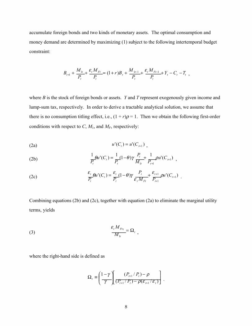
Equation (5) gives the optimal allocation condition of two different currencies. It is easily

verified that ∂Ωt/∂(εt+1/εt) > 0. Thus, under an assumption of sticky prices, devaluation of the

foreign exchange rate will have the household switch domestic currency holdings to foreign

currency holdings. In order to see this optimal condition from a viewpoint of currency

substitution, let us define the foreign-currency-preference variable, α, as follows:

(4a) M1t = (1-αt) Mt

(4b) εMFt = αtMt.

This foreign-currency preference, α, is the key variable since its value, as it rises from 0 to 1,

activates progressively greater currency substitution. If α = 0, there is no currency substitution

effect and a consumer holds only the domestic currency as an asset. The condition α = 0 is also

satisfied in the case of non-convertibility of the domestic currency and strict capital control. In

either case, foreign money holding is forced to be zero. On the other hand, the case of α = 1

indicates that domestic residents hold monetary assets exclusively in the form of foreign money.

This is the case of complete dollarization. Hence, the variable α reflects the degree of softness of

a currency, defined as currency substitution for asset-holding purposes. The value of α then

represents an inverse transformation of Gresham’s law since, as it ranges from 0 to 1, it is the

good (hard) currency that progressively drives out the bad.

From equations (3), (4a), and (4b), the optimal level of foreign-currency-preference, α,

becomes

(5) t

tt Ω+

Ω=1

α .

Recall that ∂Ωt/∂(εt+1/εt) > 0. Then, we can easily show that ∂αt/∂(εt+1/εt) > 0, indicating that

exchange rate devaluation will induce currency substitution under the assumption of sticky prices.

10

What happens when the prices adjust instantaneously? To see this, we assume that the

purchasing power parity (PPP) condition holds because of the instantaneous and complete price

adjustments. In this case, we have Pt = εtP*, where P* is the foreign price level which is assumed

to be constant to avoid unnecessary complications.6 Then equation (5) becomes

(5a) *

*

1 t

tt Ω+

Ω=α , where

−

−

−≡Ω+

+

)/)(1(

)/(1

1

1*

tt

ttt εερ

ρεεγγ

.

Denote that εt+1/εt = 1 + λt, where λt is devaluation rate. Then we can show that

(5b) [ ]0

)1()1(

)1)(1(2>

−+−−−≡

∂∂

ργρλργργ

λα

tt

t.

This comparative statics result indicates that currency substitution is induced by a

devaluation. Facing a depreciation of the foreign exchange rate, households optimally switch their

domestic currency to foreign currency, in order to maximize their intertemporal utility. This

result holds in general, regardless of the speed of price adjustment. Also, from equations (5a) and

(5b), it is straightforward to show that ∂αt/∂γ < 0 and ∂(∂αt/∂λt)/∂γ < 0, indicating that strong

utility preference towards the domestic currency decreases the effects of currency substitution by

lowering its level and muffling the response toward devaluations. Alternatively, a particular

utility preference toward foreign currency induces strong currency substitution as a behavioral

consequence. These results are intuitively straightforward.

3.2 The Monetary Model of Currency Crisis

Now, we can employ the conventional money demand function:

6 Our qualitative results will not change in the following relevant argument even if we assume that P* is constant.

11

(6) ),( 1+= tt

t

t iYLP

M,

where Yt is income and it is the nominal interest rate. Note that the real money demand function

can be derived from a dynamic optimization model of a household (Sidrauski, 1967; Lucas and

Stokey, 1987; Feenstra, 1986). Combining Equations (4a) and (6), we have the following

domestic money demand function:

(6b) ),()1()1( 11

+−=−= ttt

t

tt

t

t iYLP

M

P

M αα .

For the sake of expositional simplicity suppose for the time being suppose that αt is

exogenously given – an issue that we will revisit later in the nest section. We thus set aside the

endogenous structure of equation (5a). Now we draw on the first generation models of Krugman

(1979), as log-linearized by Obstfeld and Rogoff (1996), to model a small open economy with a

foreign exchange rate that complies with purchasing power parity (PPP) and uncovered interest

parity (UIP). This model assumes perfect goods market and capital mobility: 7

(7a) pt = et + pt*

(7b) it+1 = it+1* + Etet+1 - et,

where e is the logarithm of the nominal exchange rate of this economy. The log of the price level,

Pt, is denoted by p, and the interest rate is denoted by i. We assume a continuous-time Cagan-

type money demand function. Then, using Equation (6b), the money market equilibrium

condition becomes:

(8) m1t – pt = log (1-αt) + φyt - ηit+1,

7 This strong assumption will be released in the empirical implementation of the model below.

12

where φ and η are income elasticity and semi-interest elasticity of money demand, respectively.

Combining (7a), (7b), and (8), we have a dynamic equation of the exchange rate which

satisfies PPP, UIP, and money market equilibrium:

(9) m1t – φyt - et + ηit+1* - pt* = log(1-αt) - η(Etet+1 - et),

Under the assumption of the small open economy, foreign variables are exogenously given. In

order to simplify the argument, we assume that - φyt + ηit+1* - pt* = 0. Then we have a

continuous version of the exchange rate dynamics under perfect foresight as follows:

(9a) mt – et = log(1-αt) - η te&

3.3 The Role of the Central Bank

The balance sheet of the Central Bank is represented as

(10) BH + εAF = MB

where BH represents the domestic government bond ownership of the Central Bank and AF is its

total foreign asset holdings, i.e., foreign bonds and reserve currency. The Central Bank’s

monetary base is M1 = µ MB, where µ > 1 represents the money multiplier. Hence, Equation (10)

gives

(11) M1 = µ (BH + εAF),

3.4 The Collapse of the Fixed Exchange Rate Regime

From Equation (9a), we can see that a fixed exchange rate regime generates

(12) m1t – e = log(1-αt).

13

Suppose that the Central Bank is required to finance an ever-increasing fiscal deficit by

buying government bonds thus expanding its nominal holdings of domestic government debt, BH.

If the growth rate of domestic bond stock is constant at λ, we have

(13) HH BB =& λ.

Following Krugman (1979), we can calculate the shadow exchange rate under the flexible

exchange rate assumption and no foreign reserves, i.e., AF = 0. In this situation, the Central

Bank’s balance sheet equation (11) implies that

(14) Htt bm += µlog1 ,

where bH indicates the log of the central bank’s bond holding. By combining Equations (13) and

(14), it becomes obvious that the money supply increases at the constant rate λ after the collapse

of the fixed exchange rate regime, i.e., λ=tm1& . Moreover, from Equation (9a), we can easily see

that λ== tt em && 1 along the balanced growth path. Therefore, inserting Equation (14) into

Equation (9a), we obtain

(15) bHt – et = - log µ + log(1-αt) - ηλ

Finally, we can derive the log of the shadow exchange rate, which is defined as the floating

exchange rate that would prevail if the fixed exchange rate regime collapsed, as follows:

(16) et = bHt + log µ - log(1-αt) + ηλ.

We can see that ∂et /∂α > 0. This indicates that the currency substitution effects due to agents’

preference toward foreign currency will induce potential devaluation of the exchange rate over

time. As a result, controlling for the fundamentals, the collapse of the fixed exchange rate would

14

occur earlier. We can formally derive the time path to the collapse as follows. From Equation

(12), we have

(17) 0HHt bb = + λ t,

where bH0 is the initial value of the central bank’s government bond holding. Combining

Equations (16) and (17), together with eT = e , we can derive the time elapsed to the collapse of

the fixed exchange rate regime as follows:

λαµ )1log(log0 tHbe

T−+−−= − η.

Hence, we can easily inspect that ∂T/∂α < 0. Again, the softness of a currency is negatively

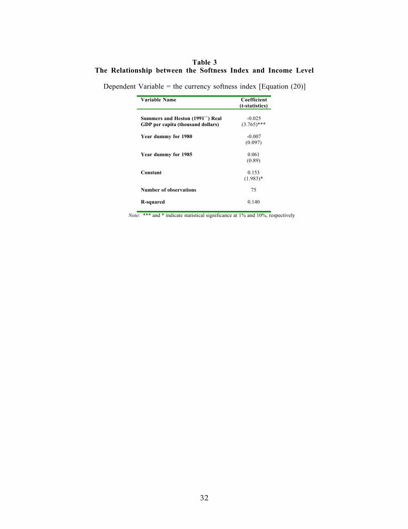
related to the timing of the currency crisis. As indicated in Figure 1, eT is the cross-over point

from fixed to flexible exchange rate, indicating devaluation. The equation and figure denote that

exogenous currency substitution, totally independently of the fundamentals and induced by shift

in preference parameters, will lead to an early collapse of the stable exchange rate regime (Figure

1).8 For example, such a change in the substitution parameter, α, can be induced by a preference

shift from domestic currency to foreign currency, i.e., a decrease in γ (equation 5a). It is

important to note that even with a modest expansion in the level of government indebtedness, λ, a

large currency substitution effect, α, can accelerate the onset of the crisis. This is applicable to

the recent Asian crises where the government account was in balance and otherwise the

fundamentals were solid (Yotopoulos and Sawada, 1999).

The intuition behind this result should be straightforward. A high degree of currency

substitution results in shrinking the demand for the domestic currency (Equation 6b). Given the

flow of money supply, a decline in money demand will increase the equilibrium price level.

According to the PPP, Equation (6), this increased price level will lead to devaluation. Although

8 Note that the first generation currency crisis model a la Krugman (1979) is the special case of our model with no

15

the devaluation rate itself will be the growth rate of the money supply, it is the currency

substitution that shifts the locus of the shadow exchange rate toward the devaluation.

So far, for the sake of tractability, we have assumed that the currency substitution

variable, α,is exogenously given. Yet, equation (5a) indicates that this variable is endogenously

determined by a household’s dynamic optimization behavior. The true equilibrium exchange rate

behavior should take into account this endogeneity of the currency substitution variable.

According to equation (5a) and (5b), there is a habit-formation of currency substitution, and thus

the foreign-currency-preference variable will increase in response to a devaluation, i.e., α = α (λ)

with ∂α/∂λ>0, because of endogeneity of the currency substitution variable, α. Then once a

country’s currency behaves as a soft currency, the dynamic locus of shadow exchange rate line,

represented by Equation (16), will be shifted toward further devaluation (Figure 1). This

mechanism creates the possibility of self-validating devaluation spirals. Soft currencies depreciate

systematically because of the currency substitution effect and crises occur more frequently. This

is a simple reduced form representation of the Y-Proposition (Yotopoulos, 1996, 1997).

3.5 Speculative Attacks and Policy Implications

The implication of the model is that even under a prudent fiscal policy and with pristine

economic fundamentals, strong currency substitution precipitates a devaluation that may turn

into a financial crisis. The premise of the analysis is that currency is held as an asset in the

utility function, regardless of the motivation for holding such an asset, whether it is for portfolio

diversification, speculation or hedging. The case of speculative attack on a currency, as made in

the literature, is related to financial capital flows in the form of “hot money.” This is a special

case of the currency-substitution-induced devaluation in the model.

A free currency market, where devaluation may happen, or it may not, provides a one-

way-option to the holder of the soft currency: by substituting the hard currency for the soft,

there is a capital gain to be reaped if devaluation happens, while there is not an equivalent loss if

currency substitution effects, i.e., α = 0.

16

it does not. This one-way bet is also offered to the “speculator” who can sell short the soft

currency. It is especially attractive to foreign fund managers who can borrow the soft currency

locally by leveraging a few billion dollars’ deposit into a peso loan with the proceeds also

converted into dollars. This play of draining the Central Bank’s reserves makes the devaluation

of the peso a self-fulfilling prophecy. And when devaluation comes, the international investor

can pay back the loan in cents on the dollar and take his hot money across the Rio Grande.9 The

entire process is initiated by taking advantage of the free currency market to convert a soft-

currency monetary asset into hard currency, thus asymmetrically increasing the asset-demand for

the latter and leading to the depreciation of the former.

The underlying asymmetry in reputation between the soft and the hard currency has a

parallel in the literature of incomplete credit markets for reasons of asymmetric information

(Stiglitz and Weiss, 1981). The policy implication of rationing foreign exchange and imposing a

mildly repressed exchange rate replicates the need for credit controls for circumventing the “bad

competition” and the “race for the bottom” that competitive price-setting implies for the credit

market. Capital controls become necessary in the case of the incomplete foreign exchange market

only to the extent that financial capital contributes to currency substitution of the soft local

currency. Otherwise, there is no need for imposing restrictions on direct foreign investment

inflows or on current account outflows for settling current account imbalances, or repatriation of

capital and profits (Yotopoulos, 1996, 1997; Yotopoulos and Sawada, 1999).

At a time when most of international capital inflows take the form of increased short-term

bank deposits, a sudden reversal of the inflows may quickly result in bank insolvencies and

failures (Calvo, Leiderman, Reinhart, 1993). Hence, a government in an attempt to prevent an

overheated credit expansion in the financial sector might opt to insulate the banking system from

short-term capital inflows. High reserve requirements are the operational policy intervention to

this effect. For example, a 100 percent required reserve ratio could be imposed on deposits with

9 A variant of this approach, fine-tuned for the existence of a Monetary Board, was used by fund managers in HongKong in September 1998. By selling short the Hang Seng stock market and at the same time converting HK dollarsinto US dollars they helped deplete the Monetary Board’s reserves thus forcing a monetary contraction. The increasein interest rates that followed fuelled a shift in assets from stocks to bonds, and a sharp decline in the stock marketthat rewarded the speculators with profits on their shorts. The scheme came to an abrupt end when the Hong Kong

17

the shortest maturity. Although this scheme would impose a burden on the banking system and

could result in some dis-intermediation of the capital inflows, it has the advantage of decreasing

banks’ exposure to the risks of sudden reversals of capital flows.

Besides controlling flows of financial capital, a conservative fiscal and monetary policy

will enable a soft-currency country to avoid a currency-substitution-led devaluation. Tightening

monetary policy, for example, by targeting reserve requirements, will contribute to avoiding

a currency crisis. To verify this argument, note that a lower money multiplier will put off the

timing of the collapse of the fixed exchange rate regime since ∂T/∂µ < 0. Recall that the money

multiplier is defined as

drc

c

D +++= 1µ ,

where c, rD, and d represent the currency-deposit ratio, the required reserve ratio, and the excess

reserve-deposits ratio, respectively. Therefore, we can easily see that increasing the required

reserve ratio will postpone the BOP crisis.

In fact, the use of reserve requirements as an appropriate financial-sector reform and an

adjustment device against capital inflows has been widely discussed recently (Cole and Slade,

1998; Calvo, Leiderman, and Reinhart, 1993). Many countries with a problematic financial sector

experience ineffective or inappropriately low reserve requirements. This leads domestic banks to

undertake risky projects that ultimately result in bank insolvencies. On the other hand, prudent

reserve requirements contribute to reducing the risks of private banks through imposing high

capital-to-risk-asset ratios and thus inducing banks to hold low-risk assets. Moreover, the central

bank can use the rent created by this operation to cover capital deficiencies in the event that

banks became insolvent and need arises to have them merged, sold, or liquidated (Cole and Slade,

1998).

4. Empirical Implementation of the Model

authorities intervened in support of the stock market (Yotopoulos and Sawada, 1999).

18

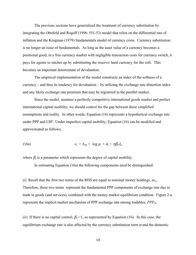
The previous sections have generalized the treatment of currency substitution by

integrating the Obstfeld and Rogoff (1996: 551-53) model that relies on the differential rate of

inflation and the Krugman (1979) fundamentals model of currency crisis. Currency substitution

is no longer an issue of fundamentals. As long as the asset value of a currency becomes a

positional good, in a free currency market with negligible transaction costs for currency switch, it

pays for agents to ratchet up by substituting the reserve/ hard currency for the soft. This

becomes an important determinant of devaluation.

The empirical implementation of the model constructs an index of the softness of a

currency – and thus its tendency for devaluation – by utilizing the exchange rate distortion index

and any likely exchange rate premium that may be registered in the parallel market.

Since the model, assumes a perfectly competitive international goods market and perfect

international capital mobility, we should control for the gap between these simplified

assumptions and reality. In other words, Equation (16) represents a hypothetical exchange rate

under PPP and UIP. Under imperfect capital mobility, Equation (16) can be modified and

approximated as follows:

(16a) et = bHt + log µ + αt + ηβ1λ,

where β1 is a parameter which represents the degree of capital mobility.

In estimating Equation (16a) the following components need be distinguished:

(i) Recall that the first two terms of the RHS are equal to nominal money holdings, m1t.

Therefore, these two terms represent the fundamental PPP components of exchange rate due to

trade in goods (and services), combined with the money market equilibrium condition. Figure 2-a

represents the implicit market mechanism of PPP exchange rate among tradables, PPPTt.

(ii) If there is no capital control, β1 =1, as represented by Equation (16). In this case, the

equilibrium exchange rate is also affected by the currency substitution term α and the domestic

19

money supply (Figure 2-b).

(iii) If there is strict capital control and foreign exchange is limited to the international trade of

goods, then β1 > 1 (Figure 2-c). As represented by Figure 2-c, under strict capital control against

short-term potfolio investments, the available amount of foreign exchange in the market is limited.

The existence of the currency substitution-driven demand for foreign exchange bids up the

equilibrium level of foreign exchange rate. The resulting foreign exchange rate is the black market

exchange rate, BM, which is higher than the equilibrium nominal exchange rate under perfect

capital mobility in Figure 2-b:

(16b) BMt = ln PPPTt + αt + β,

where PPPTt is the fundamental PPP part and β represents the degree of capital control.

(iv) Since the official nominal exchange rate (NER) is usually managed by the government in soft-

currency countries, the previous cases need reflect the official NER. BM, in specific, does not

necessarily represent the official NER. BM is regarded as the logarithm of the black market

exchange rate which reflects the existence of currency substitution by the domestic residents and

foreign exchange market interventions of the governments. Finally, subtracting NER from the -

both sides of (16b), we have the empirical model of currency substitution variable or the currency

softness index αit:

(18) BMit - ln NERit = ln PPPTit – ln NERit + β Dit +αit.

Let BP denote the black market premium relative to the nominal exchange rate. Then, by

applying a first-order Taylor expansion to equation (18), we have

(19) BPit = ln DNERit + β Dit +αit,

20

where ln DNERit=1n PPPTit – ln NERit. If data sets are available, the currency softness index, αit,

can be derived as the residual of this empirical model, by regressing the log of black market

premium, BPit, on the NER distortion index, ln PPPTit – ln NERit, and the capital control indicator

variable, Dit, which takes value of one if there are any foreign exchange controls and zero

otherwise.

Equation (19) calls for imposing coefficient restrictions. We thus estimate Equation (19)

with coefficient restriction on the NER distortion index by using OLS with the Huber-White

robust standard error. The regression version of equation (19) is:

(19a) (BPit - 1n DNERit ) = β Dit +αit.10

Finally, we obtain the currency softness index, αit, as the estimated residuals of Equation (19a).

4.1 The Data Set

In order to estimate the regression equation (19a), we need three variables: the foreign-

exchange-rate black-market premium BP; the nominal exchange rate (NER); the distortion index

1nDNER; and qualitative information about foreign capital control.

First, the data for the rate black market premium on the foreign exchange rate are widely

available from different sources. We utilized a comprehensive annual cross-country panel data set

of black market premium, which is compiled by Adrian Wood (1999). This data set covers 42

countries over a period of ten years (Table A2).

Second, consistent annual panel information on exchange rate restrictions is reported in

Ernst & Whinney (various years)11. They report restrictions on equity capital; debt capital;

interest; dividends and branch profits; and royalties, technical service fees, etc. Based on these

reports, we can easily construct a binary variable of foreign capital control.

10 We also add time effects in this regression.11 Ernst and Young since 1989.

21

However, obtaining the appropriate NER distortion index that the theory requires is not

easy. The empirical version of the NER distortion index that is broadly used for gauging a

currency's tendency to appreciate or depreciate is supposed to measure the deviation of the

nominal exchange rate (NER) from the ideal world where PPP holds and the prices of tradables

tend to converge internationally (McKinnon, 1979). The empirical application of the index,

however, whether it relies on the differential rate of inflation or other shortcut methods, reflects

the prices of both tradables and nontradables. Measuring the deviation of the NER, which is

formed exclusively in the world of tradables, by using a (PPP-deflated) general price index

introduces a distortion that makes the resulting index of questionable value. This shortcoming is

remedied by utilizing the unique set of data on the prices of tradables alone that Yotopoulos

(1996) has developed.

Yotopoulos' point of departure is the PPP exchange rate that is constructed from the

price-parity (micro-ICP) data of the Penn World Tables (Summers and Heston, 1991). The

familiar expression that gives purchasing power parity, PPP, for country I as the geometric

average of the k GDP-exhaustive commodity categories, is

(20)

∑

=

=∏=

k

i

Ii

Ii QQ

k

iW

i

IiI

P

PPPP

1

1

where PiI and Pi

W are the prices of i homogeneous commodity for country I and for the numeraire

country (world), and Q are the quantity weights.

Different aggregations of Equation (20) can lead to alternative price indexes, such as the

national price level of consumption or of government expenditure. For the Yotopoulos

application the normalized index of the prices of tradables is constructed as:

(21)

∑

=

+=∏+=

T

Ni

Ii

Ii QQ

T

NiW

i

Ii

TP

PP

1

1

where i = N + 1, ..., T is defined for commodities that are tradable in country I, (and

22

symmetrically for i = 1, ..., N for the nontradables). The PPP indexes in equation (21) are

expressed in local currency per US (numeraire country) dollar.

It still remains to be determined how to delineate the two subsets of commodities, i = 1,

..., N and i = N+1,...,T. Tradability is certainly related to tradedness. It could therefore be

defined based on the empirical-positivist rule of whether a good enters (international) trade or not.

One could then define two mutually exclusive categories of traded and nontraded goods. This

heuristic approach, however, fails to address some important issues. Is any participation in

international trade sufficient to make a good tradable? If so few nontradable goods would

probably remain. Empirically the issue is addressed by resorting to the standard definition of

openness in an economy that involves the ratio of imports and exports to GDP. The binary

classification into tradables and nontradables was made by adopting an arbitrary cut-off point of

trade value (the sum of exports and imports) for a commodity group of 20 percent of the total

commodity expenditure in GDP. By distinguishing a large number of commodity groups and by

weighting both prices and the participation of each individual commodity into tradability by

actual expenditure weights, we have effectively blunted the arbitrariness of the criterion.

Implementation of the definition of the real exchange rate (RER) relies on the micro-PPP

data of the ICP (Kravis, Heston, and Summers, 1982; Penn World Tables). For the "basic

classification" prices and nominal and real per capita expenditures (expressed in domestic

currency per U.S. dollar) are available for 152 GDP-exhausting commodities for the "benchmark"

countries and years. They were used in a flexible aggregation form to derive prices of tradables

and nontradables. The data for the definition of tradability come from the United Nations

Yearbook of International Trade Statistics which provides in 5-digit SITC classification for each

country the value of exports (f.o.b.) and imports (c.i.f.) in U.S. dollars. The 5-digit classification

was re-aggregated to achieve concordance with the ICP data. Appendix Table A1 presents the

value of the index for prices of tradables for the benchmark countries that were included in at least

one of the phases II, III, IV, and V of the ICP for 1970, 1975, 1980, and 1985, respectively.

Let a variable NER represent a country’s nominal exchange rate (NER) expressed in local

currency/US dollar. A country i’s tradable goods price at time t is represented by PTit. Let PPPT

23

denote the PPP level of tradable goods, i.e.,

=

TtUS

TitT

itP

PPPP

,

. Then, as we have discussed

already, we can define a NER distortion index, DNER, as follows:

(22) ,it

Tit

itNER

PPPDNER ≡

where T is a superscript for tradables. The ratio of tradable prices in the parentheses represents

an implicit long-run equilibrium purchasing power parity of tradable prices. Therefore, uit

represents the nominal exchange rate distortion, which is defined as the deviation of NER from the

PPP for tradable goods, i.e., the long-run equilibrium exchange rate. We can then formulate

formally:

Proposition (NER Misalignment): If DNERit>1 or ln DNERit>0, then the NER isovervalued relative to the purchasing power parity level; and if DNERit<1 or ln DNERit<0,then it is undervalued. If there are no time-specific and country-specific distortions, thenabsolute PPP holds among tradables.

Proof: From Equation (22), if DNERit > 1 ⇔ T

itit PPPNER < , NER is overvalued, and if

DNERit < 1 ⇔ T

itit PPPNER > , NER is undervalued. Moreover, if DNERit = 1 ⇔T

itit PPPNER = . Q.E.D.

Therefore, we can simply estimate this NER distortion index from Equation (22) by taking

the ratio of the relative price level of tradables to the NER, i.e.,

(22a)

=

it

Tit

itNER

PPPDNER lnln .

Note that the index takes the value of zero if there is no NER distortion. In order to quantify this

measure of distortion, we take advantage of Yotopoulos’ (1996) estimates of PPPT/ε that rely on

the price parities (micro-ICP) data set. The resulting estimates of NER distortions are also

24

presented in Appendix Table A1.

4.2 Estimation Results of the Currency Softness Index.

The summary statistics of the empirical estimation are presented in Table 1.

The estimation results of equation (19a) are presented in Table 2. As we can see, the

exchange control has a positive and significant coefficient. This is consistent with the theoretical

prediction which says that foreign capital controls will increase a country’s foreign exchange black

market premium (Figure 2-c). Another finding is that the dummy for 1985 has a positive and

significant coefficient. This year-specific positive effect probably represents the impact of the

significant appreciation of US dollar in the early 1980s and the resultant systematic depreciation

of other countries’ currency toward the US dollar.

We can derive the softness index by utilizing the framework of equation (20). The

estimated results are summarized in Table A2. Although the data set and the episodes of

currency crises are not rich enough to statistically investigate causality of our currency-

substitution hypothesis, we can empirically examine its relevance to crises by other methods. In

order to characterize empirically the currency softness, we employ two different approaches.

First, the relationship between the softness measure and the currency distortion index is

represented in Figure 4. We can clearly see that Figure 4 indicates a negative relationship between

the constructed currency softness index and the degree of NER overvaluation. The fact that soft

currencies are more likely to be undervalued (i.e., too many pesos to the dollar) is consistent with

the theoretical expectation of the model. The operational difference between a hard and soft

currency is that the exchange rate for the latter reflects not only the demand and supply of foreign

exchange for transaction (balance-of-payments) purposes, but includes also an additional splice of

“precautionary” demand for foreign exchange to be held as an asset. To the extent that hard-

currency-country residents do not need to hedge their domestic money-asset holding by

accumulating soft currency, the latter is bound to devalue. The tendency then for soft currencies

to have “high” nominal exchange rates in Equation (22) drives the DNER values below 1 (and to

negative territory) thus indicating an undervalued domestic currency. This is consistent with the

25

finding of Yotopoulos (1996: Chapter 6) in the original study of exchange rate parity relying on

micro-PPP data. Also, we can easily see that capital control is negatively related with the

currency substitution/softness indicator, α, which is fully consistent with our theoretical

framework in Section 2.1.

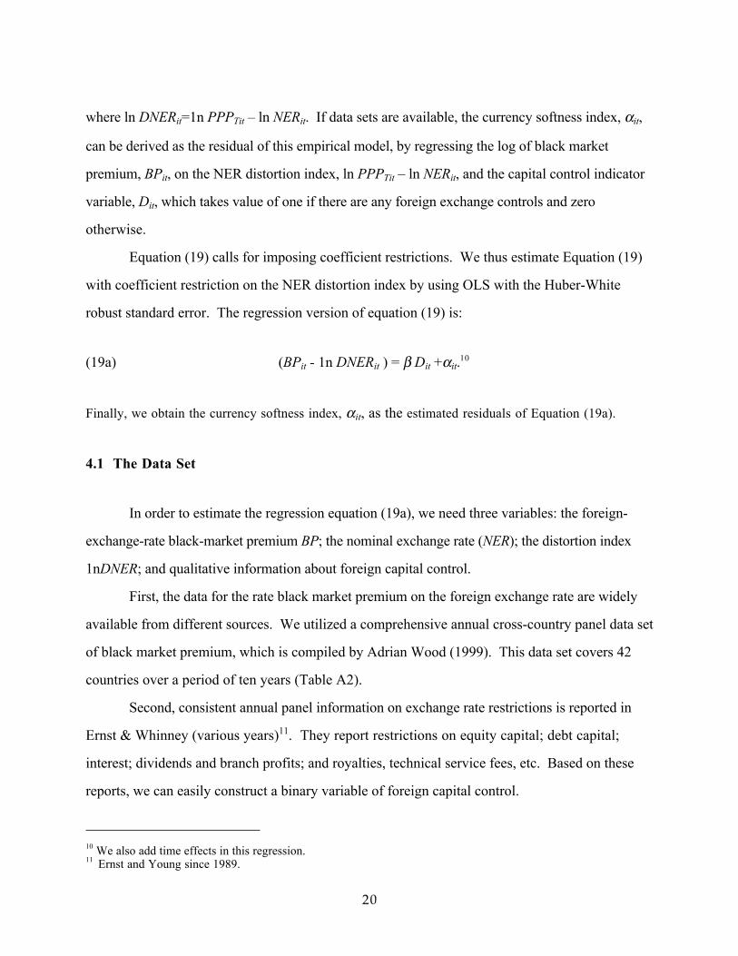
The second empirical finding relates to the negative relationship between the currency

softness index and per capita real GDP as is verified in Figure 5.12 To examine this relationship

statistically, we regressed the estimated currency softness index on the per capita GDP. We also

included the year dummy variables in order to control for a potential bias due to year-specific

systematic effects. The estimation results are presented in Table 3. The coefficient on per capita

GDP is negative and highly significant. This result confirms that there is a systematic

relationship between the credibility of a currency and the level of economic development. This

argument is consistent with the story that a less-developed country is more likely to be subject to

systematic devaluations due to its reputation-challenged currency. In fact, there might be a

circular causation between a currency's softness and a country’s low level of economic

development. When not constrained by controls, residents in a poor economy prefer holding the

dollar because the domestic currency lacks in its credibility. A poor country finds it difficult to

establish its currency’s reputation because of the low level of economic development. There

might be a certain two-way causality, which implies a vicious circle for a country's economic

development.

The obverse side of this finding holds that the best way for a soft currency to acquire

reputation and therefore to behave like a hard currency is for development to succeed. In other

words, liberalizing the currency market as a policy intervention for promoting development

amounts to putting the horse in front of the cart. A currency cannot become hard by behaving

like a hard currency, i.e., by trading freely in the world’s exchange markets. There is an

appropriate sequence in the process of economic liberalization. Freeing the foreign exchange

market comes towards the end of this process when the main business of development has been

done (Yotopoulos, 1996: Chapter 11).

12 Data on per capita real GDP is extracted from Summers and Heston (1991) Penn World Tables.

26

5. Conclusions

Since 1980 three-quarters of member-countries of the IMF, developed, developing, and

emerging alike, have been hit by financial crises. In the 1990s financial crises have become

especially virulent occurrences. The “fundamentals” models of financial crises can still do service

with an increasing dose of willing suspension of disbelief.

This paper extends the first-generation models of financial crises to allow for a systematic

devaluation of soft currencies that is independent of the fundamentals of an economy. In a

globalized world of free foreign exchange rates and free capital movements, the demand for

racheting up the quality of a currency used as an asset increases. Currency substitution in favor

of the reserve currency (currencies) becomes an exogenous factor relating to currency as a

positional good, and leads to systematic devaluation of the soft currency – and eventually to

crises.

The theoretical model and its empirical validation establish that the softness of a currency

is a most important determining factor of the likelihood of a devaluation. Moreover, per capita

income and the level of development are inversely related to the currency substitution variable

that quantifies a currency’s softness. The foreign exchange control variable moderates a

currency’s softness and its tendency to end up undervalued (“too many” pesos to the dollar) in a

free currency market. Besides (or barring) foreign exchange controls, a “moderately repressed

exchange rate” can be achieved by controlling and moderating the inflow of short-term capital,

thus avoiding systematic devaluations of soft currencies. Regulation of the banking sector serves

the same end. By setting, for example, higher reserve requirements the money multiplier is

lowered thus improving banks’ capital-to-risk-asset ratio. In sum, the policy recommendations of

the paper refer to the means of achieving “moderately repressed exchange rates,” and thus helping

diffuse the pressure for devaluation of soft currencies, in a globalization environment where

reserve and soft currencies compete for asset placement in agents’ portfolia.

28

References

Agénor, Pierre-Richard (1994), “Credibility and Exchange Rate Management in DevelopingCountries,” Journal of Development Economics, 45 (October): 1-15.

Barro, Robert J. and David B. Gordon (1983), “Rules. Discretion and Reputation in a Model ofMonetary Policy,” Journal of Monetary Economics, 12 (July): 101-121.

Blanchard, Oliver and Stanley Fischer (1989), Lectures on Macroeconomics. Cambridge, MA:MIT Press.

Baumol, William (1952), “The Transactions Demand for Cash: An Inventory TheoreticApproach,” Quarterly Journal of Economics, 66: 545-556.

Calvo, Guillermo A. and Carlos Végh (1996), “From Currency Substitution to Dollarization andBeyond: Analytical and Policy Issues,” in Guillermo A. Calvo, Money, Exchange Ratesand Output. Boston, MA: MIT Press.

Calvo, Guillermo A., Leonardo Leiderman, and Carmen M. Reinhart (1993), “Capital Inflows andReal Exchange Rate Appreciation in Latin America,” IMF Staff Papers, 40 (1): 108-151.

Cole, David C. and Betty F. Slade (1998), “The Crisis and Financial Sector Reform,” ASEANEconomic Bulletin, 15 (3): 338-346.

Eichengreen, Barry, Andrew K. Rose, and Charles Wyplosz (1994), “Speculative Attacks onPegged Exchange Rates: An Empirical Exploration with Special Reference to the EuropeanMonetary System.” NBER Working Paper No. 4898.

Ernst & Whinney (various years), Foreign Exchange Rates and Restrictions.

Feenstra, Robert (1986), “Functional Equivalence between Liquidity Costs and the Utility ofMoney,” Journal of Monetary Economics, 17: 271-291.

Flood, Robert and Peter Garber (1984), " Collapsing Exchange Rate Regimes: Some LinearExamples," Journal of International Economics, 17 (August): 1-13.

Frank, Robert H. (1985), Choosing the Right Pond. New York: Oxford University Press.

Frank, Robert H. and Philip J. Cook (1976), The Winner-Take-All Society: Why the Few at theTop Get So Much More Than the Rest of Us. New York: Penguin.

29

Girton, Lance and Don Roper (1981), “Theory and Implications of Currency Substitution,”Journal of Money, Credit and Banking, 13 (1): 12-30.

Giovannini, Alberto and Bart Turtelboom (1994), “Currency Substitution,” in Frederick van derPloeg, ed., The Handbook of International Macroeconomics. Oxford: Basil Blackwell.

Hirsh, Fred (1976), Social Limits to Growth. Cambridge, MA: Harvard University Press.

Kareken, Johm and Neil Wallace (1981), “On the Indeterminacy of Equilibrium Exchange Rates,”Quarterly Journal of Economics, 96 (2): 207-222.

Keynes, John Maynard (1923), A Tract for Monetary Reform. New York: Macmillan.

Kravis, Irving B., Alan Heston and Robert Summers (1982), World Product and Income:International Comparisons of Real Gross Product. Baltimore, MD: Johns Hopkins.

Krugman, Paul R. (1979) “A Model of Balance-of-Payments Crises,” Journal of Money, Creditand Banking, 11: 311-25.

Lucas, Robert and Nancy L. Stokey (1987), “Money and Interest in a Cash-in-AdvanceEconomy,” Econometrica, 55 (May): 491-513.

McKinnon, Ronald.I. (1979), Money in International Exchange. New York: Oxford UniversityPress.

Obstfeld, Maurice and Kenneth Rogoff (1996), Foundations of International Macroeconomics.Cambridge, MA: MIT Press.

Pagano, Ugo (1999), “Is Power an Economic Good? Notes on Social Scarcity and the Economicsof Positional Goods,” in Samuel Bowles, Maurizio Franzini and Ugo Pagano, eds., ThePolitics and Economics of Power. London: Routledge. Pp. 63-84.

Sidrauski, Miguel (1967), “Rational Choice and Patterns of Growth in a Monetary Economy,”American Economic Review, 57 (2): 534-544.

Stiglitz, Joseph E. and Andrew Weiss (1981), "Credit Rationing in Markets with ImperfectInformation," American Economic Review, 71 (June): 393-410.

Summers, Robert and Alan Heston (1991), “The Penn World Table (Mark 5): An Expanded Setof International Comparisons, 1950-1988,” Quarterly Journal of Economics, 106 (May):327-368. Homepage: http://pwt.econ.upenn.edu/

Tobin, James (1956), “The Interest Rate Elasticity of Transactions Demand for Cash,” Review of

30

Economics and Statistics, 38: 241-247.

Wood, Adrian (1999), "Data on Black Market Premium." University of Sussex, Institute ofDevelopment Studies (Compact Disk).

Yotopoulos, Pan A. (1996), Exchange Rate Parity for Trade and Development: Theory, Tests,and Case Studies. London and New York: Cambridge University Press.

Yotopoulos, Pan A. (1997), “Financial Crises and the Benefits of Mildly Repressed ExchangeRates.” Stockholm School of Economics Working Paper Series in Economics and Finance,No. 202 (October).

Yotopoulos, Pan A. and Yasuyuki Sawada (1999), “Free Currency Markets, Financial Crises andthe Growth Debacle: Is There a Causal Relationship?” Seoul Journal of Economics, 12(4): 419-456..

31

Table 1Summary Statistics

Variable Name Mean(Standard deviation)

Black market premium (%) 4.03(.57)

Yotopoulos’ exchange rate distortion index -0.171(0.304)

Per capita GDP 6781.64(3884.00)

Number of observations 75

Table 2Estimation of the Currency Softness Index

[Equation (19a)]Dependent Variable = modified black market premium

Variable Name Coefficient(t-statistics)

Capital control dummy( =1 if foreign capital is controlled)

0.458(7.70)***

Year dummy for 1980 0.018(0.23)

Year dummy for 1985 0.293(3.90)***

Constant -0.118(1.863)*

Number of Observations 75R-squared 0.491

Note) *** and * indicate statistical significance at 1% and 10%, respectively

32

Table 3The Relationship between the Softness Index and Income Level

Dependent Variable = the currency softness index [Equation (20)]

Variable Name Coefficient(t-statistics)

Summers and Heston (1991``) RealGDP per capita (thousand dollars)

-0.025(3.765)***

Year dummy for 1980 -0.007(0.097)

Year dummy for 1985 0.061(0.89)

Constant 0.153(1.983)*

Number of observations 75

R-squared 0.140

Note: *** and * indicate statistical significance at 1% and 10%, respectively

33

Figure 1

Timing of the Crisis

eT Equation (16)

α=α (λ)>0

e

0 bHT bH

34

Figure 2-aDetermination of Equilibrium PPP Exchange Rate

Through International Trade of Goods

Foreign exchange rate Supply of foreign currency

by export sector

PPPTt

Demand of foreign currencyby import sector

0Demand and supply of foreign currency

35

Figure 2-bDetermination of Equilibrium Exchange Rate

Under PPP and Perfect Capital Mobility


by export sector

Equilibrium exchange rate

PPPTt

Additional demand due to currency substitutionof domestic residents


0Demand and supply of foreign currency

36

Figure 2-cDetermination of Equilibrium Exchange Rate

Under PPP and Strict Capital Control


by export sector

BM

PPPTt

Additional demand due to currency substitutionof domestic residents

Official NER


0

Available foreign exchange in the market Demand and supply of foreigncurrency

37

Figure 4Currency Softness Index and Nominal Exchange Rate Distortion Index

(Pooled data of 1975, 80, and 85)

Softness Index

NER Distortion Index (ln DNER)

With Capital Control Without Capital Control

-1.008 .346

-.700

.623

Undervaluation Overvaluation

Note: The above table does not contain the samples with BP=0. In these cases, the softness index and the NERdistortion index are linearly dependent by construction.

38

Figure 5Currency Softness Index and Level of Economic Development

(Pooled data of 1975, 80, and 85)

Softness Index

Per Capita Real GDP (1980 dollar)

With capital control Without capital control

632 15264

-.700

.623

Argentina (1980)

39

Table A1Basic Data Based on Micro ICP

Country(Data Quality)

YEAR RPL(T) NER dist. Per capita GDP

PPPT/e ln DNER RGDPCHAustralia A- 1985 0.884 -0.123 12422.6Austria A- 1985 0.824 -0.194 10322.2

Belgium A 1985 0.811 -0.209 10617.4

Canada A- 1985 0.887 -0.120 15264.4

Denmark A- 1985 0.968 -0.033 11685

Finland A- 1985 1.017 0.017 11221.2

France A 1985 0.854 -0.158 11489.8

Germany A 1985 0.862 -0.149 11671.8

Greece A- 1985 0.653 -0.426 5614

Hungary B 1985 0.412 -0.887 5328

India C 1985 0.595 -0.519 696.6

Ireland A- 1985 0.816 -0.203 6031

Jamaica C 1985 0.552 -0.594 2393

Japan A 1985 1.037 0.036 10907

Kenya C 1985 0.411 -0.889 859

Netherlands A 1985 0.771 -0.260 10937

New Zealand A- 1985 0.763 -0.270 9848.6

Norway A- 1985 1.112 0.106 13521

Poland B 1985 0.507 -0.679 3844

Portugal A- 1985 0.604 -0.504 4643

Spain A- 1985 0.696 -0.362 6605

Sweden A- 1985 1.01 0.010 12158

Turkey C 1985 0.365 -1.008 3317

Uk A 1985 0.76 -0.274 10715

(Source) Background estimation of Yotopoulos (1996), Summers and Heston (1991)

40

Table A1Basic Data Based on Micro ICP (continued)



PPPT/e ln DNER RGDPCHArgentina C 1980 1.414 0.346 4437

Austria A- 1980 1.163 0.151 9453.4

Belgium A 1980 1.198 0.181 10248.4

Bolivia C 1980 0.82 -0.198 1852

Canada A- 1980 0.847 -0.166 13713.8

Chile C 1980 0.914 -0.090 4045

Colombia C 1980 0.577 -0.550 3392

Costa Rica C 1980 0.826 -0.191 3827

Dom Rep C 1980 0.801 -0.222 2250

Ecuador C 1980 0.668 -0.403 3092

El Salvador C 1980 0.7 -0.357 1898

France A 1980 1.224 0.202 11088.8

Germany A 1980 1.26 0.231 10850.4

Greece A- 1980 1.038 0.037 5408

Guatemala C 1980 0.645 -0.439 2574

Honduras C 1980 0.766 -0.267 1376

Hungary B 1980 0.636 -0.453 5034

India C 1980 0.489 -0.715 641

Ireland A- 1980 1.065 0.063 6150

Israel B 1980 0.966 -0.035 8369

Italy A 1980 1.023 0.023 9714

Japan A 1980 1.181 0.166 9534

Kenya C 1980 0.628 -0.465 951

Korea Rp B- 1980 0.719 -0.330 3174

Mexico C 1980 0.692 -0.368 5621

Netherlands A 1980 1.179 0.165 10503.2

Norway A- 1980 1.292 0.256 11635.8

Panama C 1980 0.763 -0.270 3368

Peru C 1980 0.436 -0.830 3141

Philpnes C 1980 0.688 -0.374 2026

Portugal A- 1980 0.813 -0.207 4439

Spain A- 1980 0.939 -0.063 6476

U.K A 1980 1.054 0.053 9696.4

Venezuela C 1980 0.921 -0.082 7000

Yugoslavia B 1980 0.983 -0.017 4551


41




PPPT/e ln DNER RGDPCHAustria A- 1975 1.186 0.171 8331.6Belgium A 1975 1.183 0.168 9326.2

Colombia C 1975 0.504 -0.685 2861

Denmark A- 1975 1.397 0.334 9433.2

France A 1975 1.214 0.194 9950.6

Germany A 1975 1.293 0.257 9634.2

India C 1975 0.614 -0.488 632

Ireland A- 1975 0.941 -0.061 5568.2

Italy A 1975 1.055 0.054 8088.6

Jamaica C 1975 0.998 -0.002 3174

Japan A 1975 0.946 -0.056 8053

Kenya C 1975 0.933 -0.069 938

Malaysia C 1975 0.626 -0.468 3217

Mexico C 1975 1.07 0.068 4671

Netherlands A 1975 1.179 0.165 9702.8

Philippines C 1975 0.711 -0.341 1764

Spain A- 1975 0.821 -0.197 6434.6

U.K A 1975 0.969 -0.031 8943

Yugoslavia B 1975 0.901 -0.104 3689


42




PPPT/e ln DNER RGDPCH

Belgium A 1970 0.863 -0.147 7764.8

France A 1970 0.913 -0.091 8458.8

Germany A 1970 0.974 -0.026 8506.2

India C 1970 0.57 -0.562 648

Italy A 1970 0.874 -0.135 6817.8

Japan A 1970 0.802 -0.221 6544

Kenya C 1970 0.514 -0.666 801

Korea B- 1970 0.502 -0.689 1712

Malaysia C 1970 0.445 -0.810 2435

Netherlands A 1970 0.827 -0.190 8362

Philippines C 1970 0.617 -0.483 1499

U.K. A 1970 0.745 -0.294 7992.4


43

Table A2Basic Data for Estimating the Relationship between Income Level and Currency Softness

Country Black MarketPremium (%)

Year NER DistortionIndex

Per CapitalReal GDP

Dummy forCapital Control

CurrencySoftness Index

Country bmp year ln DNER Rgdpch Control alpha

Argentina 0.33 1980 0.346 4437 1 -0.70

Australia 0.00 1985 -0.123 12422.6 0 -0.05

Austria 0.00 1975 0.171 8331.6 0 -0.05

Austria 0.00 1980 0.151 9453.4 0 -0.05

Austria 0.00 1985 -0.194 10322.2 0 0.02

Belgium 0.00 1975 0.168 9326.2 0 -0.05

Belgium 0.00 1980 0.181 10248.4 0 -0.08

Belgium 0.00 1985 -0.209 10617.4 0 0.03

Bolivia 22.00 1980 -0.198 1852 1 0.06

Canada 0.00 1980 -0.166 13713.8 0 0.27

Canada 0.00 1985 -0.12 15264.4 0 -0.06

Chile 5.90 1980 -0.09 4045 1 -0.21

Colombia 4.26 1975 -0.685 2861 1 0.39

Colombia 1.14 1980 -0.55 3392 1 0.20

Costa Rica -0.48 1980 -0.191 3827 0 0.29

Denmark 0.00 1975 0.334 9433.2 0 -0.22

Denmark 0.00 1985 -0.033 11685 0 -0.14

Dom Rep 10.74 1980 -0.222 2250 1 -0.03

Ecuador 13.00 1980 -0.403 3092 1 0.18

Finland 0.00 1985 0.017 11221.2 0 -0.19

France 0.00 1975 0.194 9950.6 0 -0.08

France 0.00 1980 0.202 11088.8 0 -0.10

France 0.00 1985 -0.158 11489.8 0 -0.02

Germany 0.00 1975 0.257 9634.2 0 -0.14

Germany 0.00 1980 0.231 10850.4 0 -0.13

Germany 0.00 1985 -0.149 11671.8 0 -0.03

Greece 7.43 1980 0.037 5408 1 -0.32

Greece 9.61 1985 -0.426 5614 1 -0.11

Guatemala 22.00 1980 -0.439 2574 1 0.30

Honduras 0.00 1980 -0.267 1376 1 -0.09

Hungary 40.34 1980 -0.453 5034 1 0.50

Hungary 36.96 1985 -0.887 5328 1 0.62

India 9.06 1975 -0.488 632 1 0.24

India 5.30 1980 -0.715 641 1 0.41

India 16.66 1985 -0.519 696.6 1 0.05

44

Table A2 (continued)Basic Data for Estimating the Relationship between Income Level and Currency Softness

Country Black MarketPremium (%)

Year NER DistortionIndex

Per CapitalReal GDP

Dummy forCapital Control

CurrencySoftness Index

Country bmp year ln DNER Rgdpch Control alpha

Ireland 0.00 1980 0.063 6150 0 0.04

Ireland 0.00 1985 -0.203 6031 0 0.03

Ireland 0.00 1975 -0.061 5568.2 0 0.18

Israel 0.66 1980 -0.035 8369 1 -0.32

Italy 0.00 1975 0.054 8088.6 1 -0.39

Italy 0.00 1980 0.023 9714 1 -0.38

Jamaica 21.98 1975 -0.002 3174 1 -0.12

Jamaica 12.86 1985 -0.594 2393 1 0.09

Japan -0.05 1975 -0.056 8053 0 0.17

Japan 0.00 1980 0.166 9534 0 -0.07

Japan -0.82 1985 0.036 10907 0 -0.22

Kenya 8.35 1975 -0.069 938 1 -0.19

Kenya 21.91 1980 -0.465 951 1 0.33

Kenya 5.53 1985 -0.889 859 1 0.31

Korea Rp 10.47 1980 -0.33 3174 1 0.08

Malaysia 0.00 1975 -0.468 3217 0 0.59

Mexico 0.00 1975 0.068 4671 1 -0.41

Mexico 3.18 1980 -0.368 5621 1 0.04

Netherlands -1.90 1975 0.165 9702.8 0 -0.07

Netherlands -2.13 1980 0.165 10503.2 0 -0.09

Netherlands -1.05 1985 -0.26 10937 0 0.07

New Zealand 0.00 1985 -0.27 9848.6 0 0.09

Norway 0.00 1980 0.256 11635.8 0 -0.16

Norway 0.00 1985 0.106 13521 0 -0.28

Panama 0.00 1980 -0.27 3368 0 0.37

Peru -0.05 1980 -0.83 3141 1 0.47

Philippines 13.18 1975 -0.341 1764 1 0.13

Philippines 3.29 1980 -0.374 2026 1 0.05

Portugal 1.62 1980 -0.207 4439 1 -0.13

Portugal -1.35 1985 -0.504 4643 1 -0.14

Spain 0.00 1975 -0.197 6434.6 1 -0.14

Spain 0.00 1980 -0.063 6476 1 -0.29

Spain 0.00 1985 -0.362 6605 1 -0.27

Sweden 0.00 1985 0.01 12158 0 -0.19

Turkey -10.15 1985 -1.008 3317 1 0.27

U.K. 0.00 1975 -0.031 8943 0 0.15

U.K. 0.00 1980 0.053 9696.4 0 0.05

U.K. 0.00 1985 -0.274 10715 0 0.10

Venezuela 0.00 1980 -0.082 7000 1 -0.28

Yugoslavia 13.14 1980 -0.017 4551 1 -0.21

Currency Substitution, Speculation, and Financial … · substitution of the reserve/hard currency...

Documents

Transcript of Currency Substitution, Speculation, and Financial … · substitution of the reserve/hard currency...