Currency Returns, Credit Risk and its Proximity: Evidence ... · Currency Returns, Credit Risk and...

Currency Returns, Credit Risk and its Proximity:

Evidence from Sovereign Credit Default Swap*

Byunghoon NamUniversity of Washington

November 2017

Abstract This paper examines whether credit risk and its proximity are priced in currencyreturns by making use of information in the term structure of sovereign credit default swap(CDS). Building upon and modifying a CDS pricing model, we construct two risk measuresexplaining different aspects of risk perception – “risk level”, measured by the level of CDScurve, represents whether the expected loss given credit events is high or low, and “riskproximity”, measured by the slope of CDS curve, captures how soon a specific credit eventis likely to be materialized. Combining with asset pricing models for defaultable bonds andexchange rate, we set up the model where exchange rate is determined by credit risk leveland proximity. Using a broad data set between 2004 and 2017 for 20 countries, we showthat risk level and proximity individually can explain considerable amount of variation incurrency returns and two risk measures together improves the predictive ability over a singleCDS spread. Comparing the two, risk level broadly plays a stronger role during normaltimes, while risk proximity gains its significance when financial crisis is near in time. Thesefindings suggest that not only credit risk level but also its proximity should be considered tobetter understand the exchange rate dynamics.

J.E.L. Codes: E43, F31, G12, G15

Keywords: Exchange Rates, Sovereign Credit Default Swap, Term Structure, Risk Proximity

* Correspondence: Department of Economics, University of Washington, Seattle, WA 98195;

[email protected].

1 Introduction

A large literature has documented the role of risk premium in explaining currency returns.

As currency can be viewed as a class of financial assets in international portfolios, systematic

sources of risk drive currency returns both across currencies and over time. Since investors

with risky currencies should be compensated for bearing risk, whether risk is high or low –

“risk level”– forecasts returns to holding that currency. Another aspect of risk that investors

are aware of is whether risk is near or far in time – the so-called “risk proximity”.1 If

a specific risky event is likely to be realized anytime soon, withdrawal of investment and

portfolio re-balancing cause changes in the value of currency. Although both aspects of risk

are perceived by investors and thus priced in currency returns, little attention has been paid

to “risk proximity”. This paper aims to evaluate the roles of these two different aspects of

risk in explaining the currency movements by using the information embedded in the term

structure of sovereign credit default swap.

Sovereign credit default swap (CDS) is a bilateral Over-the-Counter (OTC) insurance

contract offering protection against the default of a referenced sovereign government. Pro-

tection buyer purchases insurance against contingent credit events by paying an annuity

premium quarterly or bi-annually and protection seller compensates buyers for the losses

given credit events.2 Similar to other insurance contracts, CDS premium or spread natu-

rally provides information about the riskiness of a referenced entity, in our case a sovereign.

Sovereign credit risk is closely related to currency risk. Intuitively, one of the biggest risk

when holding financial assets issued in foreign currency is sovereign credit risk. Credit event

such as a default may trigger a collapse of the banking system of a country, causing enormous

losses on the value of assets denominated in that currency. Under floating exchange rate

regime and free capital flow, obviously the price of insurance against credit events measures

sovereign and currency risk well. Many researches empirically find that sovereign CDS

spread reflects the market pricing of time-varying systematic risk from various origins. Pan

and Singleton (2008) and Longstaff et al. (2011) show that global risk is a main driver

of CDS spread, while Remolona et al. (2008) argue that local risk is also an important

determinant. Stability of domestic financial system is also found to affect the CDS spread

(Acharya et al., 2013).

1The term “risk proximity” is often used in risk management literature.2In practice, there is no default in government bond. Instead, International Swap and Derivative Associa-

tion (ISDA) references four types of credit events: acceleration, failure to pay, restructuring, and repudiation.Sovereign CDS has been increasing in use from early 2000s and as such, policy makers, regulators and in-vestors monitor CDS spreads to gauge national financial stability. See Appendix for details about contractualprovisions and statistics.

1

Sovereign CDS spread has advantage over other risk measures because it is directly

observable. As currency risk is not observable, there have been several alternative approaches

to circumvent this issue. Pioneered by Lustig and Verdelhan (2007), many finance literature

on the carry-trade strategy consider systematic exchange risk as unobserved common factor.3

They empirically show the portfolio constructed by the carry-trade strategy yields high

returns due to latent risk measures. Another approach estimates currency risk by borrowing

risk information from the other asset classes. Bekaert et al. (2007) point out that risk factors

driving the premiums in the term structure of interest rates may also drive the risk premium

in currency returns. Similarly, Chen et al. (2017) theoretically and empirically show that

bond term premiums, which are separated out from the yield curve, are linked to currency

risk premiums. Compared to these risk measures, sovereign CDS spread, by nature, is free

from issues related to nonobservance and estimation because it is an observable price of credit

risk determined by the interaction of protection buyers and sellers in the market. Recent

researches in the aftermath of major global crises consider sovereign CDS as risk measure

and relate to the carry-trade returns (Coudert and Mignon, 2013; Corte et al., 2014).4

Another useful feature of sovereign CDS to be pointed out is its term structure. There ex-

ist different sovereign CDS contract tenors from 1- to 10-years and all the tenors are actively

traded in the market, unlike corporate CDS which is mostly concentrated in 5-year tenor

contract.5 Borrowing the concept of bond yield curve, we can construct the term structure

of sovereign CDS and define CDS curve as CDS spreads against tenors. We pay attention

to the term structure because it delivers more useful information over an single asset price

as proven from recent researches. They attempt to explain currency movements in the net

present value (NPV) framework by using the information from the term structures. Clarida

et al. (2003) show that the term structure of FX forward premiums succeeds in predicting

future spot exchange rates, while a single forward rate fails. Similarly, Chen and Gwati

(2014) find that FX option term structure contains information about higher moments in

exchange rate dynamics and helps forecast the currency returns. For the term structure of

interest rates, as it embodies information about the time-varying risk as well as the expec-

tation about future macroeconomic fundamentals, cross-country yield curve differences are

examined to explain the currency behavior well (Chen and Tsang, 2013; Chen et al., 2017).

While this line of research has shown that the measures extracted from the term structures

3The carry-trade is a strategy under which investors take long positions on high-yield currency and shortpositions on low interest rate currency. Other papers following this approach are Brunnermeier et al. (2009),Farhi et al. (2009), Lustig et al. (2011), Menkhoff et al. (2012) and many.

4Earlier work of Reihart (2002) also explores the effect of sovereign default events on currency crises,using credit rating data.

5See Appendix for details about statistics.

2

improve the forecasting ability, studies on what exactly these measures represent and how

they drive the currency returns are scant. This paper explicitly investigates the implications

of risk measures from CDS term structure and links to exchange rates by building a CDS

pricing model and combining with insights from previous researches on exchange rates and

defaultable bonds.

We first present the reduced-form model of CDS pricing where CDS spread is determined

by current and expected future path of risk-free short rates, default probabilities and frac-

tional losses given default over contract tenor. In order to summarize the term structure

of CDS spreads and the shape of CDS curve, level and slope factors are constructed in the

spirit of Nelson and Siegel (1987). Graphically, level captures the co-movement of various

tenors of CDS spreads and slope reflects the gap between shortest- and longest-tenor CDS

spreads. Interpreting the expressions for level and slope of CDS curve based on the CDS

pricing model, we coin them as “risk level” and “risk proximity”, respectively. Level of CDS

curve is expressed as the weighted average of expected losses given default over different

horizons. As an increase in level implies that expected losses, regardless of contract tenors,

are escalated due to either higher default probabilities or larger loss rates, we can name it as

risk level. Slope, defined as shortest- minus longest-tenor CDS spreads, provides information

about the timing of credit events. We prove that if default probability in the long-run is

higher than in the short-run, CDS curve is upward-sloping and slope is negative. Conversely,

inverted CDS curve and positive slope are resulted from relatively higher default probability

in the near term. In this regard, higher value of slope captures how soon the credit event is

likely to be materialized – the so-called risk proximity.

We then link credit risk measures to currency returns by well-known finance literature.

Applying the asset pricing model for defaultable bonds (Duffee and Singleton, 1999), we show

that stochastic discount factor or pricing kernel is written as a function of risk-free rates,

default probabilities and losses given default. Following Backus et al. (2001) that relate

the ratio of home and foreign pricing kernels to exchange rate changes under no arbitrage

condition, we iterate forward this relation to get the net present value (NPV) equation where

exchange rate is determined by cross-country differences in pricing kernels in the current and

future periods. Combining two, we demonstrate that exchange rate is determined by current

and expected future path of risk-free rates, default probabilities and losses given default at

home and abroad. Since this information is also contained in CDS spreads from short to

long tenors and effectively summarized by level and slope of CDS curve, connection between

credit risk measures and currency returns can be well-established. Therefore, theoretically,

currency return should be determined by both credit risk level and proximity.

3

For the empirical test, we look at a broad data set of quarterly exchange rate changes

against USD, three-month zero-coupon yields and the term structure of sovereign CDS for

twenty countries from 2004 to 2017. Our sample countries mostly consist of emerging and

developing countries because credit risk is particularly potential in these countries, compared

to advanced countries. We first check if level and slope factors capture most of variation in

entire sovereign CDS spreads of various tenors. Principal Component Analysis reveals that

the first two principal components, which explain almost all of the variation in CDS curve,

actually represent graphical level and slope respectively. Then, we proceed to examine the

roles of different sets of sovereign credit risk measures including a single CDS spread, level

and slope factors in explaining the exchange rate changes. The results confirms the existing

findings in the recent finance literature as follows: 1) sovereign credit risk forecasts a large

share of subsequent currency returns (Coudert and Mignon, 2013); 2) the effect of risk on

currency movements is state-dependent (Clarida et al., 2009 among many) – an increase

in sovereign credit risk results in positive currency returns under low volatility state, while

leads to low returns or losses under high volatility state6; 3) the UIP puzzle is mitigated

by reducing the omitted variable problem once incorporating credit risk measures in the

regression.

This paper is distinctive in the following dimensions: 1) level and slope factors individu-

ally can explain considerable amount of the variation in currency movements; 2) the model

with both level and slope factors outperform the model with a single CDS in explanatory

power. These findings suggest that not only risk level but also risk proximity matters for

currency returns and should not be ignored. Our results are similar to yet distinguished

from previous term structure literature. While confirming that the term structure of an

asset delivers more useful information about risk in addition to a single asset price, we make

a progress by clearly interpreting that new information from the term structure is about

different aspects of risk perception of market participants – risk level and proximity. To my

knowledge, there has been no attempt to investigate the role of risk proximity in driving

asset prices. Considering that investors are sensitive to how soon a bad event is actually

likely to happen as well as how much the expected loss is, the concept of risk proximity

may be one of the missing pieces in asset pricing model in general; 3) Comparing the role of

risk level and proximity, the former explains currency behavior more consistently, while the

latter catches up its role near the crises.

6Clarida et al.(2009) divide the sample periods into high, medium, low volatility and find that highinterest rate currency pays high return during low volatility times, but low return during high volatilitytimes. These results coincide with the findings in Brunnermeier et al. (2009) that under adverse financialmarket, as the carry-trades are unwound, dramatic depreciation happens for the high interest rate currency.

4

2 Theoretical Framework

2.1 Price of Credit Default Swap

In order to explore the informational contents contained in the term structure of CDS,

we start by evaluating a price at time t of an m-tenor CDS (Dmt ).7 Building upon and

modifying continuous time pricing of CDS in Duffie et. al. (2003), we set up the pricing

model in discrete time framework in order to analytically examine the meaning of CDS

spreads and its term structure. The premium leg which is the present value of protection

buyer’s cash flow (V PBt ) is given by8

V PBt = Dm

t + htexp(−rt)0 + (1− ht)exp(−rt)Et(V PBt+1 ) (1)

where rt is risk-free short rate at time t, ht is default probability between time t and t + 1

conditional on information up to time t, and lt is expected fractional loss at t+1 conditional

on information up to time t. The CDS premium (Dmt ) is paid at the beginning of time

t for the protection. If a credit event is triggered between time t and t + 1, the contract

is terminated and no more premium is paid. If not, the contract goes on to next period.

Iterating forward the eq.(1), we get9

V PBt = Dm

t Et

[m∑j=0

exp

(−

j∑k=0

(rt+k−1 + ht+k−1)

)](2)

On the other hand, the contingent payment leg which is the present value of protection

seller’s cash flow (V PSt ) is given by

V PSt = htexp(−rt)lt + (1− ht)exp(−rt)Et(V PS

t+1) (3)

If credit event is materialized between time t and t+1, the protection seller pays the notional

amount equivalent to the loss given event at the end of time t+ 1, terminating the contract.

7We use the term “tenor” instead of “maturity” for CDS contract because the length of CDS contract isshorter than or equal to underlying bond maturity and the cash flow of CDS is fundamentally different fromthat of bond.

8We assume without loss of generality that CDS premium is paid on a yearly basis. This assumptionenables us to relate annualized CDS spreads to annualized exchange rate changes and interest rate. However,the model can easily be translated into bi-annual or quarterly payment schemes.

9We define rt−1 = ht−1 = 0 and use the approximation of exp(c) ' 1 + c, for small c.

5

Iterating forward the eq.(3), we get

V PSt = Et

[m∑j=1

exp

(−

j∑k=1

(rt+k−1 + ht+k−2)

)ht+j−1lt+j−1

](4)

Granted that a fairly priced CDS at time t equates V PBt and V PS

t , a price at time t of an

m-tenor CDS (Dmt ) is expressed as

Dmt =

Et

[∑mj=1 exp

(−∑j

k=1(rt+k−1 + ht+k−2))ht+j−1lt+j−1

]Et

[∑mj=0 exp

(−∑j

k=0(rt+k−1 + ht+k−1))] (5)

A single CDS spread of tenor m is a function of current and expected future path of risk-free

short rates, default probabilities and fractional losses given default over the same tenor. So,

we can rewrite the equation using general functional form (g(.)) as:

Dmt = g(Rm

t , Hmt , L

mt ) (6)

whereRmt = [rt, Etrt+1, ..., Etrt+m]′, Hm

t = [ht, Etht+1, ..., Etht+m]′, Lmt = [lt, Etlt+1, ..., Etlt+m]′.

2.2 Risk Level and Risk Proximity

To make use of information embedded in the term structure of CDS in effective and

parsimonious way, we describe the shape of CDS curve with level and slope factors, borrowing

the idea from bond yield curve model (Nelson and Siegel, 1987 among others).10 Suppose

sovereign CDS has tenors of m = 1, 2, ..., n. Level factor is defined as a CDS spread of the

longest tenor, L(Dt) = Dnt , and slope factor as the difference in CDS spreads between the

shortest- and the longest-tenor, S(Dt) = D1t −Dn

t . The meaning of level factor is straight-

forward. From eq.(5), it represents the weighted average of expected losses given default

over short to long horizons. The weights for each period are just different from conventional

discount rates. Since expected loss measures whether the risk embedded in that asset is

high or low, let us refer to it as “risk level”. An increase in level implies expected losses,

regardless of contract tenors, are escalated due to either higher default probabilities or larger

loss rates.

Now, let’s examine the implication of slope factor. To motivate the idea with simple

10In Section 3, from Principal Component Analysis, we show that level and slope factors are actually thefirst two principal components which explain 99% of variation in entire CDS spreads at each time t.

6

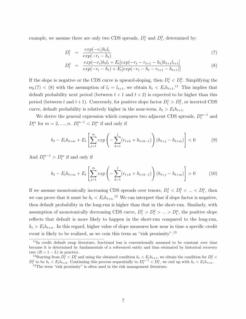
example, we assume there are only two CDS spreads, D1t and D2

t , determined by:

D1t =

exp(−rt)htltexp(−rt − ht)

(7)

D2t =

exp(−rt)htlt + Et[exp(−rt − rt+1 − ht)ht+1lt+1]

exp(−rt − ht) + Et[exp(−rt − ht − rt+1 − ht+1)](8)

If the slope is negative or the CDS curve is upward-sloping, then D1t < D2

t . Simplifying the

eq.(7) < (8) with the assumption of lt = lt+1, we obtain ht < Etht+1.11 This implies that

default probability next period (between t+ 1 and t+ 2) is expected to be higher than this

period (between t and t+1). Conversely, for positive slope factor D1t > D2

t , or inverted CDS

curve, default probability is relatively higher in the near-term, ht > Etht+1.

We derive the general expression which compares two adjacent CDS spreads, Dm−1t and

Dmt for m = 2, ...., n. Dm−1

t < Dmt if and only if

ht − Etht+m + Et

[m∑j=1

exp

(−

j∑k=1

(rt+k + ht+k−1)

)(ht+j − ht+m)

]< 0 (9)

And Dm−1t > Dm

t if and only if

ht − Etht+m + Et

[m∑j=1

exp

(−

j∑k=1

(rt+k + ht+k−1)

)(ht+j − ht+m)

]> 0 (10)

If we assume monotonically increasing CDS spreads over tenors, D1t < D2

t < ... < Dnt , then

we can prove that it must be ht < Etht+n.12 We can interpret that if slope factor is negative,

then default probability in the long-run is higher than that in the short-run. Similarly, with

assumption of monotonically decreasing CDS curve, D1t > D2

t > ... > Dnt , the positive slope

reflects that default is more likely to happen in the short-run compared to the long-run,

ht > Etht+n. In this regard, higher value of slope measures how near in time a specific credit

event is likely to be realized, as we coin this term as “risk proximity”.13

11In credit default swap literature, fractional loss is conventionally assumed to be constant over timebecause it is determined by fundamentals of a referenced entity and thus estimated by historical recoveryrate (R = 1− L) in practice.

12Starting from D1t < D2

t and using the obtained condition ht < Etht+1, we obtain the condition for D2t <

D3t to be ht < Etht+2. Continuing this process sequentially to Dn−1

t < Dnt , we end up with ht < Etht+n.

13The term “risk proximity” is often used in the risk management literature.

7

2.3 Sovereign Credit Risk and Exchange Rates

Consider a price at time t of a one-period zero-coupon government bond (P 1t ) which is

subject to default risk (Duffie and Singleton, 1999) given by

P 1t = exp(−rt − htlt) (11)

Compared to a default-free bond, a defaultable bond is like being priced using the default-

adjusted discount rate, which is essentially the nominal short rate: it = rt + htlt.14

Following many popular models of asset prices, under the absence of arbitrage, we assume

that a stochastic discount factor (SDF) or a pricing kernel of home country (Mt+1) which

prices all assets is conditionally log-normal:

Mt+1 = exp

(−rt − htlt −

1

2λ

′

tλt − λ′

tεt+1

)(12)

The term λt is time-varying price of risk associated with the sources of uncertainty εt.

Assuming that the sources of uncertainty are rt, ht and lt, we specify λt is a function of these

state variables. Equivalently, we obtain a pricing kernel of foreign country (M∗t+1) as

M∗t+1 = exp

(−r∗t − h∗t l∗t −

1

2λ∗

′

t λ∗t − λ∗

′

t ε∗t+1

)(13)

where λ∗t is a function of r∗t , h∗t and l∗t .

Now, let’s investigate the linkage between sovereign credit risk and exchange rate. Backus

et al. (2001) establish the condition under which home asset returns equate foreign asset

returns denominated in home currency as15

St+1

St=M∗

t+1

Mt+1

(14)

where St is the spot exchange rate of home currency measured as per foreign currency.

Defining the log of exchange rate st ≡ logSt and the log of pricing kernels mt+1 ≡ logMt+1,

m∗t+1 ≡ logM∗t+1, no-arbitrage requires that expected exchange rate change is given by the

expectation of difference between the log of foreign and home pricing kernels as specified in

eq.(12) and (13), so that

Etst+1 − st = Et(m∗t+1 −mt+1) (15)

14See Duffie and Singleton (1999) for discussion.15See Backus et al. (2001) for discussion.

8

Iterating eq.(15) forward in terms of st, we get a net present value (NPV) equation where

exchange rate is determined by the cross-country differences in pricing kernels in the current

and the future:

st = Et

∞∑j=1

(mt+j −m∗t+j)

= Et

∞∑j=0

[−(rt+j + ht+jlt+j − r∗t+j − h∗t+jl∗t+j)−

1

2

(λ

′

t+jλt+j − λ∗′

t+jλ∗t+j

)](16)

Assuming that λt (λ∗t ) is a function of rt, ht, lt (r∗t , h∗t , l∗t ) at each time t, exchange rate at time

t depends on current and expected future path of risk-free rates, default probabilities and

expected fractional losses at home and abroad. We can express this equation using general

functional form (h(.)) as:

st = h(Rt, Ht, Lt, R∗t , H

∗t , L

∗t ) (17)

where Rt = [rt, Etrt+1, ..., Etrt+∞]′, Ht = [ht, Etht+1, ..., Etht+∞]′, Lt = [lt, Etlt+1, ..., Etlt+∞]′,

R∗t = [r∗t , Etr∗t+1, ..., Etr

∗t+∞]′, H∗t = [h∗t , Eth

∗t+1, ..., Eth

∗t+∞]′ and L∗t = [l∗t , Etl

∗t+1, ..., Etl

∗t+∞]′.

2.4 Linking Term Structure of CDS and Exchange Rates

From the eq.(17), we have shown that exchange rate is determined by state vectors

(Rt, Ht, Lt, R∗t , H

∗t , L

∗t ). Since sovereign CDS spreads contain information about the same

state variables up to their tenors as in the eq.(6), the vectors of home CDS and foreign CDS

over entire tenors (Dt = [D1t , D

2t , ..., D

nt ]′, D∗t = [D1,∗

t , D2,∗t , ..., Dn,∗

t ]′), can be used as proxies

for these state vectors. As we demonstrated that level and slope measures effectively summa-

rize the CDS curve and provide more interesting interpretation of risk level and proximity,

we propose to use level and slope instead of entire set of CDS spreads. Then, the eq.(17),

using different general function (f(.)), becomes

st = f(L(Dt), S(Dt), L(D∗t ), S(D∗t )) (18)

Since nominal exchange rate is best approximated by a unit root process empirically, we focus

our analyses on exchange rate change, ∆st+m = st+m − st. So, we conduct the empirical

studies to show how level and slope factors of sovereign CDS curve determine subsequent

exchange rate changes in the following sections.

9

3 Basic Empirics

3.1 Data Description

Twenty sample countries are chosen on the basis of two criteria. First, sovereign CDS

should be actively traded in the market. We select candidate countries in descending order by

the trading volume reported by the Depository Trust and Clearing Corporation (DTCC).16

Second, among the candidates, we exclude the countries whose exchange rate regime is not

floating, based on the IMF Annual Report on Exchange Arrangements and Exchange Restric-

tions, 2016. Sample countries are Australia(AU), Brazil(BR), Chile(CL), Columbia(CO),

Hungary(HU), Iceland(IS), Indonesia(ID), Israel(IL), Japan(JP), Korea(KR), Mexico(MX),

Norway(NO), Peru(PE), Philippines(PH), Poland(PL), Romania(RO), South Africa(ZA),

Sweden(SE), Thailand(TH), Turkey(TR) and the United States of America(US). Although

our samples are mostly emerging and developing countries where sovereign credit risk is

especially potential, we have complete set of both advanced and emerging economies over

various continents including America, Asia, Europe, and Africa.

The main data we examine consists of monthly observations from January 2004 to June

2017 of the following series:17 1) spot exchange rate data: End-of-month exchange rates are

obtained from the Bloomberg. We use the logged exchange rate, measured as per-dollar

rate. Quarterly exchange rate change is expressed as ∆st+3 = st+3 − st and indicated as

annualized percentage. Positive ∆st+3 means the depreciation of home currency against

the US dollar and negative ∆st+3 means the appreciation; 2) zero coupon yield of three-

month maturity: End-of-month zero coupon yields as annualized percentage are obtained

from the Bloomberg.18 Then, quarterly excess currency return is computed as xrt+3 =

i3t − i3,USt − ∆st+3. Positive xrt+3 implies gain from the trade borrowing from the US and

investing in home country and negative xrt+3 represents loss; 3) sovereign CDS data: Data on

sovereign CDS spread is collected from the Bloomberg and the Datastream. We use sovereign

CDS spreads with tenors of 1, 2, 3, 5, 7, 10 years, with USD as currency of denomination

and in annuity basis point. CDS spreads are from the last trading day of each month.

Table 1 reports the summary statistics of our sample data. Considering potential struc-

tural breaks due to the Great Recession, the sample period is divided by two preliminary

16The Depository Trust and Clearing Corporation(DTCC) runs a warehouse for CDS trade confirmationsaccounting for around 90% of the total market and releases market data on the outstanding notional of CDStrades on a weekly basis.

17Sample periods are shorter for some countries due to data availability.18For countries in which zero coupon yield data is not available, three-month interbank rates are obtained

from central banks.

10

break dates – November 2007 and June 2009.19 For the interpretation purpose, we label

three sub-periods divided by two breaks as “Pre-Crisis”, “Crisis”and “Post-Crisis”. For

quarterly exchange rate change ∆st+3 in Panel A, we observe that all currencies have ap-

preciated before the Crisis except for IDR, JPY and ZAR, and all currencies except JPY

have depreciated during the Crisis. This would be consistent with the idea that the US dol-

lar (along the Japanese Yen) is commonly considered safe haven currencies. Behavior after

the Crisis is differentiated across countries due to local and domestic events. For example,

BRL, COP, HUF and ZAR have depreciated further, while ISK, ILS, KRW have appreciated.

The volatility of exchange rate has been increased during the Crisis. After the Crisis, the

standard deviation has decreased but still higher than the Pre-Crisis level for some countries

reflecting persisted uncertainties. From Figure 1, we see episodes of exchange rate volatility,

with the spike during the Great Financial Crisis and the European Fiscal Crisis. Panel B

presents statistics on excess currency returns xrt+3. Similar to exchange rate changes, most

of the countries have shown high returns before the Crisis and low returns or losses during

the Crisis.

Panel C describes the statistics on interest rate differentials measured by cross-country

differences in zero-coupon yield of three-month maturity as home minus US yield i3t − i3,USt .

Interest rate of home country is higher than that of the US and their gap has been widened

during the Crisis. The volatility is very low, compared to that of exchange rate, implying

that interest rate differential is not enough to generate the variation in currency movements

and lending support on the view why more volatile variables are needed as explanatory

variables in addition.

3.2 Principal Component Analysis of Term Structure of CDS

We describe the evolution of the term structure of sovereign CDS over sample period.

Figure 2 graphically shows sovereign CDS spreads of six different contract tenors. One

immediately noticeable feature present in all countries is that all the CDS spreads co-move.

During major global events when sovereign credit risk is mounted, CDS spreads jump up

regardless of tenors. What is more interesting in this figure is that the gap between short-

and long-tenor CDS spreads varies over time. Usually, the long-tenor CDS spread is higher

than the short-tenor CDS spread due to longer exposure and higher uncertainty, but the

gap becomes narrower or even inverted during the Global Financial Crisis. Level of CDS

19According to the NBER, the recession in the US is from December 2007 to June 2009. Although therecession periods in sample countries are not identical, we choose these breaks considering that no countrywas free from the massive impact of the Global Financial Crisis.

11

curve explains the co-movement of CDS spreads, while slope describes the difference between

the shortest- and the longest-tenor CDS spreads. From this observation, we can draw two

lessons: 1) the term structure of sovereign CDS contains more information than a single

CDS spread; 2) level and slope of CDS curve summarize the shape of CDS curve well. In

the previous section, we theoretically demonstrated that level reflects “risk level ”and that

slope captures “risk proximity”. For example, consider the case of Iceland. As Iceland has

experienced the financial crisis that involved the actual default of all three major commercial

banks in the last 2008 to 2010, instant sovereign default was highly anticipated in the market,

which was reflected in positive slope as well as skyrocketed level.

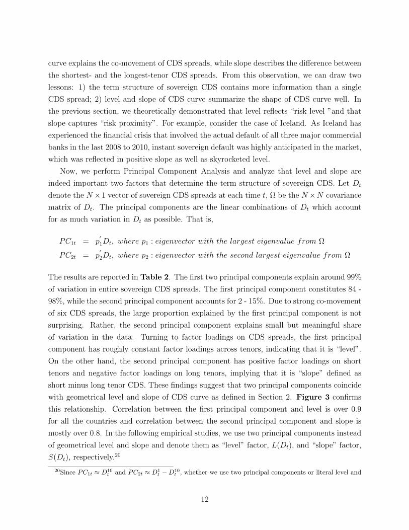
Now, we perform Principal Component Analysis and analyze that level and slope are

indeed important two factors that determine the term structure of sovereign CDS. Let Dt

denote the N ×1 vector of sovereign CDS spreads at each time t, Ω be the N ×N covariance

matrix of Dt. The principal components are the linear combinations of Dt which account

for as much variation in Dt as possible. That is,

PC1t = p′

1Dt, where p1 : eigenvector with the largest eigenvalue from Ω

PC2t = p′

2Dt, where p2 : eigenvector with the second largest eigenvalue from Ω

The results are reported in Table 2. The first two principal components explain around 99%

of variation in entire sovereign CDS spreads. The first principal component constitutes 84 -

98%, while the second principal component accounts for 2 - 15%. Due to strong co-movement

of six CDS spreads, the large proportion explained by the first principal component is not

surprising. Rather, the second principal component explains small but meaningful share

of variation in the data. Turning to factor loadings on CDS spreads, the first principal

component has roughly constant factor loadings across tenors, indicating that it is “level”.

On the other hand, the second principal component has positive factor loadings on short

tenors and negative factor loadings on long tenors, implying that it is “slope” defined as

short minus long tenor CDS. These findings suggest that two principal components coincide

with geometrical level and slope of CDS curve as defined in Section 2. Figure 3 confirms

this relationship. Correlation between the first principal component and level is over 0.9

for all the countries and correlation between the second principal component and slope is

mostly over 0.8. In the following empirical studies, we use two principal components instead

of geometrical level and slope and denote them as “level” factor, L(Dt), and “slope” factor,

S(Dt), respectively.20

20Since PC1t ≈ D10t and PC2t ≈ D1

t −D10t , whether we use two principal components or literal level and

12

Table 3 describes the statistics for level and slope factors with potential structural

breaks. During the Crisis, level has jumped up and slope has become flatter or even inverted.

This implies that investors have perceived that huge loss from the credit event is highly likely

to occur in the near future due to the impact from the Global Financial Crisis. In contrast,

slope during the Post-Crisis period has quickly become as steep as in the Pre-Crisis period,

while level has stayed up high. It can be interpreted that sovereign risk level was still high

due to sluggish recovery of real economies and on-going financial uncertainties, but actual

credit events were believed not to be realized near in time thanks to international efforts for

securing the financial safety nets.

4 Main Results

4.1 Explaining the Currency Returns with Sovereign Credit Risk

We empirically examine whether sovereign credit risk factors perceived at the particular

point in time can explain quarterly currency returns as predicted from the reduced-form

model developed in Section 2. We also compare the explanatory power of different sets of

risk measures: 1) one-year CDS spread, D1t ; 2) level factor, L(Dt), which captures risk level;

3) slope factor, S(Dt), which implies risk proximity; 4) both level and slope factors, L(Dt)

and S(Dt).21 Specifically, the following regressions are estimated with structural breaks for

each currency pairs:22

Model 1: ∆st+3 = β0 + β1D1t + εt+3 (19)

Model 2: ∆st+3 = β0 + β1L(Dt) + εt+3 (20)

Model 3: ∆st+3 = β0 + β1S(Dt) + εt+3 (21)

Model 4: ∆st+3 = β0 + β1L(Dt) + β2S(Dt) + εt+3 (22)

slope does not make a big difference to our empirical studies.21In our empirical study, we focus on home sovereign CDS spreads only. One reason is that we assume

no default risk in the US, our foreign country. This assumption is realistic in that market participantsrarely expect the default in the US assets. The other reason is that data on US sovereign CDS spreads onlybecomes available in recent years. However, later in this section, we conduct the robustness check by usingthe cross-country differences in credit risk factors.

22Test for endogenous structural breaks in the regression is performed based on Bai and Perron (2003)multiple break tests(with 15% trimming and 5 - 10% significance level). After identifying zero to two breaks,structural break dummy variables for each sub-period are incorporated into the regression.

13

Table 4 presents p-values from joint Wald test and adjusted R2s.23 As shown in the table,

p-values are all below 5% with a few exceptions for Israel and Thailand. The hypothesis that

sovereign credit risk factors have no information about three-month exchange rate change

is strongly rejected, regardless of which set of risk measures are employed. The regressions

generate high adjusted R2s up to 60%. This is quite an impressive portion in light of the

near-zero R2 typical in this literature. We confirm the existing finding that sovereign credit

risk accounts for a large share of currency returns (For example, Coudert and Mignon, 2013.).

Comparing the predictive ability of four different models, we first notice that the model

with both level and slope factors (Model 4) can explain currency movements better than

the model with one-year CDS spread (Model 1) in most countries. This finding lines up

with with previous literature that term structures provide more useful information than

a single asset price (Clarida et al., 2003; Chen and Tsang, 2013). One-year CDS spread

may capture the amount of credit risk in the shortest run, but cannot say anything about

the timing of risky events. In contrast, level and slope from the term structure of CDS,

which capture both credit risk level and proximity, can together help more comprehensively

evaluate the investors’ perception of risk and thereby better forecast the currency returns.

Another prominent feature is the performance of slope-only model (Model 3). Given that

slope factor explains only small portion of the variation in entire CDS spreads as investigated

in the Principal Component Analysis, its explanatory power is beyond expectation. This

model performs better than one-year CDS model (Model 1) in 9 out of 20 countries and

even better than level-only model (Model 2) in 8 out of 20 countries. These results lend

support on our argument that foreign currency holders care not only how much of sovereign

risk is expected from that currency, but also how near in time the risky event is expected to

happen.

We further investigate the relation between credit risk measures and currency returns by

employing two-state Markov-Switching model. Although structural break model estimates

coefficients in sub-sample periods divided by break dates, the state-dependent relationship

between variables might be averaged out in long sub-sample periods. This model is also silent

about what each state represents. Alternatively, Markov-Switching model can show the state-

dependency more clearly by allowing the regime to switch endogenously by unobserved yet

comprehensive state factors. The model specification is as follows:

23To complement our analysis of the link between sovereign credit risk and currency movements, we alsoregress excess currency returns, xrt+3 on four sets of risk measures. The results remain qualitatively thesame. The results are provided in Appendix.

14

∆st+3 = β0,ξt + β1,ξtL(Dt) + β2,ξtS(Dt) + εt+3, (23)

where εt+3 i.i.d.N(0, σ2ξt)

βi,ξt = βi,0(1− ξt) + βi,1ξt, for i = 0, 1

σ2ξt = σ2

0(1− ξt) + σ21ξt

ξt = 0, 1

Pr[ξt = 0|ξt−1 = 0] = P00

Pr[ξt = 1|ξt−1 = 1] = P11

where ξt is state variable. After estimating the parameters by Maximum Likelihood Estima-

tion (MLE), the filtered probabilities are computed by Hamilton filter (Hamilton, 1989).24

The regression results are reported in Table 5. We first observe that adjusted R2s are

very high up to 72%. Even though Markov-Switching model is estimated by Maximum

Likelihood Estimation (MLE) which maximizes the log-likelihood of the model, we can com-

pute adjusted R2s from the linear combinations of two fitted values weighted by filtered

probabilities of each state.25 26

What does each regime imply? The volatility of state 1 appears to be relatively high

compared to that of state 1 for all countries (σ20 < σ2

1). Consequently, state 0 represents

“low volatility”state, and state 1 stands for “high volatility”state. We also explore when

the volatility has been historically high by graphically checking the filtered probability of

state 1 (P1) as illustrated in Figure 5. High volatility states for sample countries com-

monly include major global crises such as the Global Financial Crisis and European Fis-

24Accurately, the model is estimated by Quasi-MLE. The model is not correctly specified because ofauto-correlation in the error term due to overlapping data. However, it turns out that MLE estimatesare consistent, while standard errors should be estimated by the robust covariance matrix. Specifically, letθ = argminθ∈Θ−lnL(θ) = argminθ∈Θ−lnf(yt; θ) and define the Gradient matrix evaluated at θ as G(θ) =∑Tt=1

∂∂θ lnf(yt; θ) =

∑Tt=1Gt, the Hessian matrix evaluated at θ as H(θ) =

∑Tt=1

∂2

∂θ∂θ′lnf(yt; θ). The robust

covariance matrix in the existence of auto-correlation can be computed by var(θ) = H(θ)−1JP (θ)H(θ)−1,

where JP (θ) =∑Tt=1GtG

′

t +∑pi=1 wi

(∑Tt=i+1GtG

′

t−i +∑Tt=i+1Gt−iG

′

t

). P indicates that the approxima-

tion is curtailed at P lags of the auto-correlation, and wi represents the weights with∑pi=1 wi = 1.

25We obtain the estimated ∆st+3 = [β0,0 + β1,0L(Dt) + β2,0S(Dt)]P0 + [β0,0 + β1,0L(Dt) + β2,0S(Dt)]P1

and compute the adjusted R2 by using the residual sum of squares (RSS).26Here, we do not report the goodness of fit measures from four different sets of risk factors as in Table

4. But, the model with both level and slope factors is also found to be superior to other models in terms ofadjusted R2 and AIC. The results can be provided upon request.

15

cal Crisis.27 Moreover, it seems noteworthy that the persistence of high volatility state is

country-dependent. The persistence is found to be low for countries like Korea, but high

for countries such as Mexico, Peru. The value transition probability from state 1 to state

1 (P11 = Pr[st = 1|st−1 = 1]) compares the country-specific persistence as it relates to the

expected duration of high volatility state by 1/(1− P11).28 The lower transition probability

(P11) a country exhibits, the longer the high volatility state persists. Economic implication

is that countries with relatively more persistent high volatility state have long struggled from

the impact of the global crises, compared to countries with less persistence.

The coefficient estimates confirm the findings from recent empirical evidences on the

carry-trade strategy (Clarida et al., 2009; Brunnermeier et al., 2009; Menkhoff et al., 2012).

They show that when the volatility is low, currency with higher risk appreciates as investors

demand compensation for holding risky currency. However, under high volatility, as investors

abruptly unwind their portfolios in favor to safe haven currency, the value of currency with

higher risk plummets. Since level and slope factors capture two types of riskiness – risk

level and proximity, an increase in either level or slope or both is accompanied by significant

appreciation of currency during low volatility state (state 0) and by depreciation or less

appreciation of currency during high volatility state (state 1).29 The concept of risk level and

proximity give insights on sign-switching relation between credit risk and currency returns

well. Recall that risk level is associated with the expected path of loss given credit events

and risk proximity delivers information about the timing of actual credit event. During

normal times when credit event is not likely to be realized shortly, both credit risk level

and proximity forecast positive currency returns, as investors still hold that currency to be

compensated for bearing risk. However, when the global crisis is about to be triggered,

country with weak economic fundamentals is vulnerable to credit risk with potential default.

Market participants with international portfolios anticipate that a default in this country

is near in time and that expected loss is also escalated due to high default probability.

Accordingly, they withdraw their investment and re-balance their portfolios so as to avoid

highly probable losses, causing depreciation in the currencies of these countries.

27Since it is difficult to clearly define exact periods for these crises, we use the Chicago Board Options Ex-change (CBOE) Volatility Index (VIX index) to identify highly volatile global financial market. Specifically,we indicate the periods when VIX index is greater than 20 along with the filtered probabilities.

28Expected duration of state 1: E(Dst=1) = sum∞j=1Pj−111 (1−P11) = 1/(1−P11). For Korea, E(Dst=1) =

1/(1− 0.780) = 4.54 months. For Mexico, E(Dst=1) = 1/(1− 0.923) = 13.01 months.29We have the similar results from the regression of the excess currency return, xrt+3. Higher level and

slope factors give high positive returns during low volatility state, and incur losses or low returns during thehigh volatility state. The results are provided in Appendix.

16

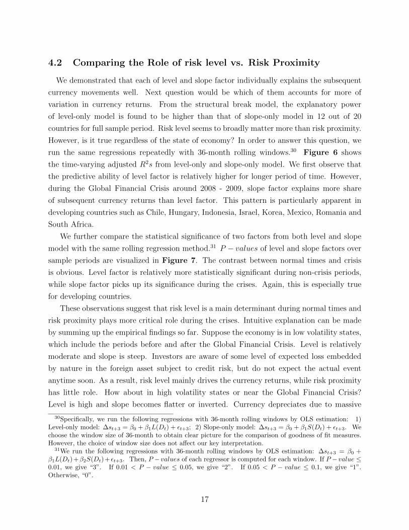
4.2 Comparing the Role of risk level vs. Risk Proximity

We demonstrated that each of level and slope factor individually explains the subsequent

currency movements well. Next question would be which of them accounts for more of

variation in currency returns. From the structural break model, the explanatory power

of level-only model is found to be higher than that of slope-only model in 12 out of 20

countries for full sample period. Risk level seems to broadly matter more than risk proximity.

However, is it true regardless of the state of economy? In order to answer this question, we

run the same regressions repeatedly with 36-month rolling windows.30 Figure 6 shows

the time-varying adjusted R2s from level-only and slope-only model. We first observe that

the predictive ability of level factor is relatively higher for longer period of time. However,

during the Global Financial Crisis around 2008 - 2009, slope factor explains more share

of subsequent currency returns than level factor. This pattern is particularly apparent in

developing countries such as Chile, Hungary, Indonesia, Israel, Korea, Mexico, Romania and

South Africa.

We further compare the statistical significance of two factors from both level and slope

model with the same rolling regression method.31 P − values of level and slope factors over

sample periods are visualized in Figure 7. The contrast between normal times and crisis

is obvious. Level factor is relatively more statistically significant during non-crisis periods,

while slope factor picks up its significance during the crises. Again, this is especially true

for developing countries.

These observations suggest that risk level is a main determinant during normal times and

risk proximity plays more critical role during the crises. Intuitive explanation can be made

by summing up the empirical findings so far. Suppose the economy is in low volatility states,

which include the periods before and after the Global Financial Crisis. Level is relatively

moderate and slope is steep. Investors are aware of some level of expected loss embedded

by nature in the foreign asset subject to credit risk, but do not expect the actual event

anytime soon. As a result, risk level mainly drives the currency returns, while risk proximity

has little role. How about in high volatility states or near the Global Financial Crisis?

Level is high and slope becomes flatter or inverted. Currency depreciates due to massive

30Specifically, we run the following regressions with 36-month rolling windows by OLS estimation: 1)Level-only model: ∆st+3 = β0 + β1L(Dt) + εt+3; 2) Slope-only model: ∆st+3 = β0 + β1S(Dt) + εt+3. Wechoose the window size of 36-month to obtain clear picture for the comparison of goodness of fit measures.However, the choice of window size does not affect our key interpretation.

31We run the following regressions with 36-month rolling windows by OLS estimation: ∆st+3 = β0 +β1L(Dt)+β2S(Dt)+ εt+3. Then, P −values of each regressor is computed for each window. If P −value ≤0.01, we give “3”. If 0.01 < P − value ≤ 0.05, we give “2”. If 0.05 < P − value ≤ 0.1, we give “1”.Otherwise, “0”.

17

withdrawal of investments from the risky assets. Which is the main driver of re-weighting

of investment from risky currencies to safe haven currencies: risk level or risk proximity?

If investors perceive that a default is far from realization although expected loss is huge

due to concurrent global devaluation of assets, they would require even more compensation

rather than unwinding the position. However, if a specific credit event is almost surely to be

immediately triggered, investors would unwind their position to avoid the losses, regardless

of risk level. As a result, the link between risk proximity and currency returns becomes more

pronounced for periods near major global crisis.

4.3 Risk-adjusted Uncovered Interest Rate Parity

This sub-section examines the role of sovereign credit risk in explaining the Uncovered

Interest Rate Parity (UIP) puzzle. Since our reduced-form model is departed from exact

UIP relation and based on the net present value (NPV) framework, we just briefly check

whether the UIP puzzle is mitigated when incorporating credit risk factors as proxies for risk

perceived at the current time t. Considering that one of the reasons for the UIP puzzle is

ignoring risk premium, we expect that inclusion of credit risk measures would help correct

the abnormal UIP coefficients. We start with the original UIP regression, which is also

known as Fama Regression (Fama, 1984). This model is used as a benchmark to compare

the results from our risk-adjusted UIP regression. We run the following regression and report

the results in Table 6:

∆st+3 = β0 + β1(it − i∗t ) + εt+3 (24)

The null hypothesis that interest rate differentials has no information about subsequent

exchange rate changes cannot be rejected and adjusted R2s are close to zero. The UIP

coefficients (β1) are negative for seven countries, while positive for the other countries. The

UIP puzzle is not as severe as in the existing empirical papers because our sample countries

are mostly emerging economies and our sample period is relatively short including major

global crises. Since our sample currencies are intrinsically risky, the deviation from the UIP

relation is smaller as implied by Bansal and Dahlquist (2000) and Frankel and Poonawala

(2010).32 In addition, as shown from summary statistics, riskier currencies tend to depreciate

more during the crisis. So, it is plausible to see positive coefficients when sample period is

exposed to severe financial turmoil. However, since our objectives is to mitigate the UIP

puzzle, we test whether the model augmented with risk premium pushes this coefficient to

32They find that the UIP coefficients are closer to 1 for emerging market currencies.

18

positive for negative coefficient countries and improves explanatory power.

Now, let us augment the UIP with risk premium, proxied by risk level (level factor) and

proximity (slope factor). The regression equation is as follows:

∆st+3 = β0 + β1(it − i∗t ) + β2L(Dt) + β3S(Dt) + εt+3 (25)

The results are reported in Table 7. Compared to the results from the original UIP, we ob-

serve some improvement. Joint Wald test that regressors have no explanatory power cannot

be rejected only for 5 countries at 10% significance level and the goodness of fit measures

increase up to 26%. We also notice improvement in the UIP coefficients. Out of seven

countries which showed negative coefficients in the UIP regression, four countries now have

positive coefficients and one country has less negative coefficient. Negative coefficients on

risk measures are also consistent with theoretical prediction. Assuming risk aversion instead

of risk neutrality, economic agents require a higher expected return on relatively riskier cross-

border investments because of risk premiums. So, when the risk premium is ignored in the

empirical regression of UIP relation, it may cause the estimators to be biased due to the

omitted variable problem (Obsfeld and Rogoff, 2001).33 In this context, after incorporating

risk premiums, measured by credit risk factors, the UIP puzzle could be mitigated.

4.4 Robustness Checks

We conduct extensive robustness checks to corroborate our key findings: 1) sovereign

credit risk measures can explain considerable amount of variation in currency returns; 2)

risk level and slope factors together explain the currency movements better than one-year

CDS – both risk level and proximity play a role in forecasting currency returns; 3) relation

between credit risk and currency returns are state-dependent; 4) risk level matters more

during normal times, while risk proximity picks up its role near crises.

Over different horizons (m = 1−, 3−, 6−, 12−months), we repeat the regressions of the

exchange rate changes on four sets of credit risk measures (eq.(19), (20)(21) and (22)) with

structural breaks. Adjusted R2 results in Table 8 are comparable to those in Table 4. All

four sets of credit risk measures can explain sizable amount of variation in currency move-

ments from monthly to yearly. Adjusted R2s are very high up to 79% in yearly prediction,

33Suppose the true model is ∆st+3 = β0+β1(it−i∗t )−ρt+εt+3, where ρt is time-varying risk premium. Riskpremium is positively correlated with interest rate differential, as risk is generally higher in higher interestrate country, and negatively correlated with the exchange rate changes, as risk premium compensates theinvestors. So, if the estimated model regresses ∆st+3 = β0 + β1(it − i∗t ) + εt+3, then β1 is negatively biased,resulting in the UIP puzzle.

19

while relatively low in monthly prediction. Comparing the explanatory powers across mod-

els, the model with both level and slope factors consistently produces the highest goodness

of fit. Markov-Switching model is also applied to different prediction horizons to check the

state-dependent property of estimates. The results for monthly prediction reported in Table

9 replicate all the findings from quarterly prediction: two regimes represent high and low

volatility states, the persistence of high volatility state is country-dependent, and coefficient

estimates are switching depending on the state of economy.

Until now, we relied on one country’s CDS spreads rather than cross-country difference in

CDS spreads when constructing credit risk measures, assuming no default risk in the US.34

However, if there exist default risk, however small it is, relative credit risk of one country to

the other should be taken into account in examining the bilateral currency movements. Here,

we relax the assumption of no default in denominating country and explore whether our main

results are preserved. Specifically, we define exchange rate against Japanese Yen. Cross-

country differences in CDS spreads between home country and Japan are used to construct

relative one-year CDS (D1,Rt = D1

t −D1,JPt ), relative level factor (L(DR

t ) = L(Dt)−L(DJPt )),

and relative slope factors(S(DRt ) = S(Dt) − S(DJP

t )).35 Using these relative measures,

we check the robustness of findings from structural break model and Markov-Switching

model. The model specifications are the same except replacing one-country risk measures

with cross-country differences. Table 10 and 11 present the results consistent with our key

findings. Whether we assume default risk in country of safe haven currency or not does not

qualitatively affect our conclusions.

We compare the explanatory power and the statistical significance of level and slope factor

with 36-months rolling windows. Voluminous regressions are performed for combinations of

four horizons (m = 1−, 3−, 6−, 12−months), two denominating currencies (USD, JPY) and

corresponding credit measures (only own country’s credit risk, relative credit risk). Figure

8 and 9 shows one example out of many results - the result from the regression of six-month

exchange rate against JPY on the relative level and slope factors. All the other results from

differently combined models are very similar. Overall, it seems safe to say that risk level

counts more, in general, while risk proximity takes a pivotal role during the crisis.

34We admit that this assumption was partly due to the lack of CDS data for the US.35Historical CDS data for Japan is available. Japanese yen is perceived as one of safe haven currencies,

while the accumulated sovereign debt is highest in the world, implying potential credit risk. In this regard,Japan is a good sample country for this robustness check.

20

5 Conclusions

This paper relates sovereign credit risk level and proximity to currency returns. Theoret-

ically, developing CDS pricing model and constructing the level and slope factors from the

term structure of sovereign credit default swap (CDS) spreads, we show that level represents

how high the expected loss is expected – risk level – and slope implies how soon the actual

credit event is likely to be realized – risk proximity. Combining with asset pricing models

for defaultable bonds and exchange rate, we set up the model where the spot exchange rate

is determined by both credit risk level and proximity. Empirically, we examine that the

explanatory power of the model with both level and slope factors improves over the model

with a single CDS spread, supporting our view that risk level and proximity capture different

aspects of risk perception of market participants. Their relative role relies on the state of

economy as risk level matters more during normal times, while risk proximity cut a con-

spicuous figure near the crises. These findings suggest that market participants and policy

authorities should closely monitor the movement of sovereign CDS spreads – not only level

but also slope of CDS curves – to better understand the short-run currency behavior.

Of course, there are many remaining tasks. Although we have restricted attention in

this paper to currency returns driven by credit risk due to clean measures of risk level and

proximity from the term structure of CDS spreads, there is no reason why these measures

cannot be obtained from the term structures of other asset classes such as bond yields and

options. By investigating the pricing mechanism of different assets, we would be able to

derive interesting interpretation from the time-varying shape of term structures. Another

next step would be to go beyond the reduced-form asset pricing model and to develop the

DSGE model. By incorporating the term structure of assets into otherwise general DSGE

open economy model, we could have more insights on the connection between macroeconomic

variables and asset prices.

21

References

[1] Acharya, V., Drechsler, I. and Schnabl, P. (2014). A pyrrhic victory? Bank bailouts and

sovereign credit risk. The Journal of Finance, 69(6), 2689-2739.

[2] Arce, O., Mayordomo, S. and Pea, J. I. (2013). Credit-risk valuation in the sovereign CDS

and bonds markets: Evidence from the euro area crisis. Journal of International Money and

Finance, 35, 124-145.

[3] Bansal, R. and Dahlquist, M. (2000). The forward premium puzzle: different tales from de-

veloped and emerging economies. Journal of International Economics, 51(1), 115-144.

[4] Backus, D. K., Foresi, S. and Telmer, C. I. (2001). Affine term structure models and the

forward premium anomaly. The Journal of Finance, 56(1), 279-304.

[5] Bai, J. and Perron, P. (2003). Computation and analysis of multiple structural change models.

Journal of Applied Econometrics, 18(1), 1-22.

[6] Bekaert, G., Wei, M. and Xing, Y. (2007). Uncovered interest rate parity and the term struc-

ture. Journal of International Money and Finance, 26, 1038-1069.

[7] Brunnermeier, M. K., Nagel, S. and Pedersen, L. H. (2008). Carry trades and currency crashes.

NBER macroeconomics annual, 23(1), 313-348.

[8] Chen, Y. C., Nam, B. H. and Tsang, K.P. (2017). Global Financial Crisis and the Exchange

Rate-Yield Curve Connection. Working paper.

[9] Chen, Y. C. and Gwati, R. (2014). Understanding Exchange Rate Dynamics: What Does The

Term Structure of FX Options Tell Us? Working paper.

[10] Clarida, R., Davis, J. and Pedersen, N. (2009). Currency carry trade regimes: Beyond the

Fama regression. Journal of International Money and Finance, 28(8), 1375-1389.

[11] Clarida, R., Sarno, L., Taylor M., and Valente G. (2003). The out-of-sample success of term

structure models as exchange rate predictors: a step beyond. Journal of International Eco-

nomics, 60(1), 61-83.

[12] Corte, P., Sarno, L., Schmeling, M. and Wagner, C. (2014). Sovereign risk and currency

returns. In The 41th European Finance Association Annual Meeting (EFA 2014).

[13] Coudert, V. and Mignon, V. (2013). The forward premium puzzle and the sovereign default

risk. Journal of International Money and Finance, 32, 491-511.

[14] Duffie, D. and Singleton, K. J. (1999). Modeling term structures of defaultable bonds. Review

of Financial studies, 12(4), 687-720.

[15] Duffie, D., Pedersen, L. H. and Singleton, K. J. (2003). Modeling sovereign yield spreads: A

case study of Russian debt. The Journal of Finance, 58(1), 119-159.

22

[16] Engel, C. (2014). Handbook of international economics (Vol. 4). Chapter 8. Elsevier.

[17] Farhi, E., Fraiberger, S.P., Gabaix, X., Ranciere, R. and Verdelhan, A. (2009). Crash risk in

currency markets. NBER working paper.

[18] Francis, C., Kakodkar, A. and Martin, B. (2003). Credit derivative handbook 2003. Merrill

Lynch, April, 16.

[19] Frankel, J. and Poonawala, J. (2010). The forward market in emerging currencies: Less biased

than in major currencies. Journal of International Money and Finance, 29(3), 585-598.

[20] Hamilton, J. D. (1989). A new approach to the economic analysis of nonstationary time series

and the business cycle. Econometrica: Journal of the Econometric Society, 357-384.

[21] Longstaff, F. A., Pan, J., Pedersen, L. H. and Singleton, K. J. (2011). How sovereign is

sovereign credit risk?. American Economic Journal: Macroeconomics, 3(2), 75-103.

[22] Lustig, H. and Verdelhan, A. (2007): The cross section of foreign currency risk premia and

consumption growth risk. The American economic review, 97, 89-117.

[23] Lustig, H., Roussanov, N. and Verdelhan, A. (2011): Common risk factors in currency markets.

Review of Financial Studies, 24, 3731-3777.

[24] Menkhoff, L., Sarno, L., Schmeling, M. and Schrimpf, A. (2012). Carry trades and global

foreign exchange volatility. The Journal of Finance, 67(2), 681-718.

[25] Nelson, C. R. and Siegel, A. F. (1987). Parsimonious modeling of yield curves. Journal of

business, 473-489.

[26] Obstfeld, M. and Rogoff, K. (2000). The six major puzzles in international macroeconomics:

is there a common cause?. NBER macroeconomics annual, 15, 339-390.

[27] Pan, J. and Singleton, K. J. (2008). Default and recovery implicit in the term structure of

sovereign CDS spreads. The Journal of Finance, 63(5), 2345-2384.

[28] Remolona, E. M., Scatigna, M. and Wu, E. (2008). The dynamic pricing of sovereign risk

in emerging markets: Fundamentals and risk aversion. The Journal of Fixed Income, 17(4),

57-71.

[29] Reinhart, C. M. (2002). Default, currency crises, and sovereign credit ratings. The world bank

economic review, 16(2), 151-170.

23

Table 1. Summary Statistics

for Exchange Rate, Excess Currency Return and Interest Rates

AU BR CL CO HU IS ID IL JP KR

Panel A: Exchange Rate Change (∆st+3)

Mean Full 0.087 0.773 0.749 0.690 2.148 2.809 3.404 -1.784 0.370 -0.207

Pre-Crisis -4.307 -13.291 -6.286 -8.658 -4.760 -2.443 2.137 -4.955 0.272 -5.525

Crisis 3.738 3.565 9.314 2.407 4.917 42.307 4.383 1.335 -9.483 16.465

Post-Crisis 1.561 7.311 2.554 5.064 5.073 -2.606 3.845 -0.819 2.433 -0.926

SD Full 27.644 33.594 23.711 28.927 30.373 33.081 20.228 16.901 21.064 22.155

Pre-Crisis 16.441 18.87 15.075 21.793 19.446 25.529 15.957 13.512 15.585 12.853

Crisis 59.086 60.240 48.206 49.812 59.310 67.001 41.599 30.490 28.362 46.174

Post-Crisis 21.895 30.072 18.802 25.486 25.931 17.587 15.349 14.467 21.420 16.458

AR(1) 0.727 0.715 0.674 0.681 0.689 0.723 0.724 0.721 0.710 0.684

Panel B: Excess Currency Return (xrt+3)

Mean Full 2.700 10.349 1.060 2.469 2.329 4.392 3.027 3.144 -1.504 2.248

Pre-Crisis 6.542 25.312 5.428 10.161 9.331 9.515 3.616 7.529 -3.578 6.364

Crisis 0.065 7.295 -4.493 5.324 3.120 -28.057 5.009 0.790 8.896 -13.401

Post-Crisis 1.296 3.411 0.973 -0.761 -1.371 8.433 2.325 2.116 -2.580 3.365

SD Full 27.475 33.727 23.918 29.681 30.628 32.227 20.589 17.344 21.033 21.917

Pre-Crisis 16.167 19.270 14.116 25.333 20.096 25.730 16.749 14.926 15.618 13.001

Crisis 58.404 59.494 47.570 49.248 59.438 67.513 41.759 30.178 28.148 45.554

Post-Crisis 22.076 30.173 18.527 25.411 26.056 17.706 15.654 14.332 21.379 16.550

AR(1) 0.725 0.717 0.653 0.673 0.691 0.704 0.722 0.712 0.711 0.675

Panel C: Interest Rate Differential (i3t − i3,USt )

Mean Full 2.746 11.081 3.111 4.462 4.377 7.146 6.403 1.211 -1.134 2.009

Pre-Crisis 2.235 12.021 0.486 2.972 4.571 7.072 5.753 0.618 -3.306 0.840

Crisis 3.803 10.860 4.821 7.731 8.037 14.251 9.392 2.125 -0.587 3.064

Post-Crisis 2.786 10.665 3.483 4.311 3.557 5.776 6.129 1.228 -0.179 2.373

SD Full 1.273 2.729 1.981 1.706 3.058 3.182 2.061 1.224 1.607 1.328

Pre-Crisis 1.188 3.737 0.801 1.301 3.200 1.959 2.230 0.808 1.303 1.202

Crisis 1.162 1.690 2.179 1.301 1.824 3.284 2.813 0.853 0.785 1.015

Post-Crisis 1.205 2.168 1.451 0.833 2.624 1.123 1.106 1.290 0.352 1.030

AR(1) 0.946 0.971 0.975 0.962 0.932 0.977 0.888 0.869 0.993 0.906

Note: 1. ∆st+3 = st+3 − st is the quarterly change of exchange rate, where st is the logged homecurrency price per USD. If ∆st+3 is positive, home currency is depreciated relative to USD. If ∆st+3 isnegative, home currency is appreciated relative to USD. 2. xrt+3 = i3t − i

3,USt −∆st+3 is excess currency

return, which is the return by investing in home currency from time t to t + 3 with funding from foreigncurrency (US). If xrt+3 is positive, the investment yields gain. If xrt+3 is negative, the investment incurs

loss. 3. i3t − i3,USt is the difference in three-month zero coupon yields or interbank interest rates in home

and foreign country (US). 4. Sample period is from January, 2004 to June, 2017. All rates are reported inannualized percentage points. 5. Sample period is divided by two break dates, November,2007 and June,2009. Sub-periods are reported as “Pre-Crisis”, “Crisis”and “Post-Crisis”, respectively. The break dates arechosen, considering the recession in the US is from December, 2007 to June, 2009 according to the NBER.

24


for Exchange Rate, Excess Currency Return and Interest Rates

(Continued)

MX NO PE PH PL RO ZA SE TH TR

Panel A: Exchange Rate Change (∆st+3)

Mean Full 3.856 1.423 -0.508 -0.856 -0.234 1.632 5.126 1.123 -1.043 7.380

Pre-Crisis -0.726 -6.906 -4.315 -8.176 -12.310 -7.396 2.268 -4.303 -4.622 -3.052

Crisis 13.133 7.042 0.010 10.401 11.710 11.073 3.016 7.521 2.042 14.563

Post-Crisis 4.276 4.485 1.309 0.544 3.429 4.266 7.002 2.558 0.135 11.185

SD Full 23.208 24.744 11.549 12.552 31.887 25.732 30.799 24.232 12.602 28.181

Pre-Crisis 10.312 18.470 7.998 11.808 21.866 21.315 27.972 19.032 12.886 26.331

Crisis 45.484 45.005 20.704 15.392 62.454 42.635 56.594 45.896 15.493 48.375

Post-Crisis 20.939 20.814 10.119 9.949 25.030 22.075 24.547 19.739 11.526 21.875

AR(1) 0.725 0.714 0.673 0.725 0.738 0.707 0.628 0.704 0.733 0.677

Panel B: Excess Currency Return (xrt+3)

Mean Full 0.546 -0.490 3.936 5.052 2.764 3.963 1.248 -1.082 2.264 1.778

Pre-Crisis 5.165 6.221 5.370 11.140 13.622 14.489 2.608 3.172 4.252 16.610

Crisis -6.701 -3.932 5.216 -0.839 -7.158 0.114 7.139 -5.814 -0.437 -0.157

Post-Crisis -0.308 -3.178 2.950 3.179 -0.697 -0.571 -0.644 -2.265 1.811 -2.930

SD Full 23.303 24.393 11.258 12.889 31.609 26.322 30.995 23.919 12.387 28.482

Pre-Crisis 10.913 18.712 8.291 11.868 22.234 22.915 28.281 18.968 13.049 25.852

Crisis 45.094 44.122 20.481 16.503 61.892 42.235 56.263 45.034 15.100 47.381

Post-Crisis 21.276 20.811 9.943 11.486 25.030 22.312 24.879 19.764 11.404 22.289

AR(1) 0.726 0.706 0.655 0.716 0.734 0.721 0.630 0.699 0.722 0.678

Panel C: Interest Rate Differential (i3t − i3,USt )

Mean Full 4.428 0.905 3.440 4.135 2.492 5.485 6.364 0.007 1.206 9.734

Pre-Crisis 4.439 -0.685 1.055 2.964 1.313 7.093 4.876 -1.131 -0.370 11.206

Crisis 6.432 3.110 5.226 9.562 4.552 11.186 10.155 1.706 1.605 14.406

Post-Crisis 4.025 1.246 4.254 3.634 2.661 3.569 6.342 0.228 1.899 8.318

SD Full 1.432 1.509 1.885 3.366 1.908 4.938 1.982 1.425 1.258 2.773

Pre-Crisis 1.876 1.106 0.706 2.814 2.351 6.496 1.664 1.342 0.554 1.471

Crisis 1.094 1.310 1.508 2.506 0.926 2.940 1.542 1.165 0.753 3.134

Post-Crisis 0.760 0.775 1.109 2.713 1.328 2.786 0.947 1.021 0.825 1.460

AR(1) 0.976 0.971 0.978 0.882 0.974 0.932 0.973 0.962 0.979 0.935

Note: 1. ∆st+3 = st+3 − st is the quarterly change of exchange rate, where st is the logged homecurrency price per USD. If ∆st+3 is positive, home currency is depreciated relative to USD. If ∆st+3 isnegative, home currency is appreciated relative to USD. 2. xrt+3 = i3t − i

3,USt −∆st+3 is excess currency

return, which is the return by investing in home currency from time t to t + 3 with funding from foreigncurrency (US). If xrt+3 is positive, the investment yields gain. If xrt+3 is negative, the investment incurs

loss. 3. i3t − i3,USt is the difference in three-month zero coupon yields or interbank interest rates in home

and foreign country (US). 4. Sample period is from January, 2004 to June, 2017. All rates are reported inannualized percentage points. 5. Sample period is divided by two break dates, November,2007 and June,2009. Sub-periods are reported as “Pre-Crisis”, “Crisis”and “Post-Crisis”, respectively. The break dates arechosen, considering the recession in the US is from December, 2007 to June, 2009 according to the NBER.

25

Table 2. Principal Component Analysis

for Term Structure of Sovereign Credit Default Swap Spreads


Panel A: The first Principal Component (PC1t)

Factor Loading 1Y 0.326 0.176 0.278 0.202 0.366 0.502 0.402 0.297 0.151 0.394

2Y 0.337 0.314 0.351 0.291 0.414 0.451 0.421 0.359 0.223 0.415

3Y 0.405 0.398 0.386 0.397 0.422 0.419 0.439 0.405 0.297 0.422

5Y 0.458 0.473 0.453 0.482 0.421 0.384 0.410 0.457 0.435 0.414

7Y 0.454 0.490 0.458 0.488 0.415 0.355 0.396 0.457 0.541 0.406

10Y 0.448 0.498 0.485 0.497 0.409 0.309 0.379 0.447 0.598 0.399

Explained 88.277 95.662 95.952 92.826 97.111 98.397 96.249 94.779 95.068 97.156

corr(PC1t, D10t ) 0.936 0.986 0.979 0.975 0.979 0.978 0.963 0.967 0.986 0.974

Panel B: The second Principal Component (PC2t)

Factor Loading 1Y 0.428 0.604 0.471 0.635 0.648 0.562 0.556 0.546 0.515 0.512

2Y 0.493 0.524 0.486 0.525 0.365 0.326 0.368 0.449 0.508 0.401

3Y 0.330 0.312 0.357 0.262 0.134 0.035 0.178 0.300 0.449 0.243

5Y -0.040 -0.102 -0.024 -0.099 -0.202 -0.314 -0.194 -0.102 0.148 -0.191

7Y -0.357 -0.295 -0.412 -0.275 -0.379 -0.461 -0.424 -0.370 -0.217 -0.432

10Y -0.579 -0.407 -0.494 -0.409 -0.495 -0.515 -0.553 -0.512 -0.454 -0.542

Explained 11.240 4.032 3.638 6.627 2.777 1.501 3.354 4.948 4.403 2.760

corr(PC2t, D1t −D10

t ) 0.922 0.541 0.668 0.687 0.974 0.566 0.987 0.846 0.423 0.996


Panel A: The first Principal Component (PC1t)

Factor Loading 1Y 0.353 0.245 0.300 0.281 0.306 0.393 0.314 0.297 0.293 0.375

2Y 0.391 0.313 0.389 0.348 0.376 0.423 0.363 0.344 0.344 0.418

3Y 0.409 0.385 0.421 0.407 0.405 0.423 0.400 0.392 0.391 0.438

5Y 0.432 0.471 0.445 0.458 0.447 0.413 0.446 0.465 0.456 0.428

7Y 0.433 0.485 0.445 0.455 0.449 0.402 0.456 0.463 0.467 0.406

10Y 0.426 0.488 0.430 0.466 0.447 0.395 0.451 0.458 0.466 0.380

Explained 94.952 84.182 91.443 95.159 95.512 97.231 91.700 93.910 90.816 89.679

corr(PC1t, D10t ) 0.957 0.917 0.946 0.975 0.967 0.978 0.950 0.952 0.941 0.909

Panel B: The second Principal Component (PC2t)

Factor Loading 1Y 0.530 0.368 0.543 0.648 0.536 0.605 0.620 0.418 0.535 0.595

2Y 0.415 0.479 0.443 0.440 0.435 0.384 0.428 0.549 0.440 0.381

3Y 0.250 0.414 0.266 0.218 0.277 0.134 0.221 0.276 0.335 0.146

5Y -0.094 0.078 -0.098 -0.131 -0.061 -0.232 -0.123 -0.018 -0.061 -0.185

7Y -0.389 -0.279 -0.425 -0.315 -0.359 -0.410 -0.353 -0.302 -0.353 -0.416

10Y -0.569 -0.616 -0.498 -0.472 -0.561 -0.496 -0.493 -0.597 -0.529 -0.521

Explained 4.734 14.808 7.432 4.674 4.143 2.649 7.960 5.415 8.987 9.516

corr(PC2t, D1t −D10

t ) 0.954 0.856 0.900 0.801 0.846 0.997 0.921 0.830 0.887 0.994

Note: 1. Principal components are obtained as follows: 1)Let Dt denote the 6 x 1 vector of CDS spreadsat each time t, Ω be the 6 x 6 covariance matrix ofDt; 2) The first principal component is PC1t = p

′

1Dt, wherep1 is an eigenvector with the largest eigenvalue from Ω; 3) The second principal component is PC2t = p

′

2Dt,where p2 is an eigenvector with the second largest eigenvalue from Ω. 2. “Factor loadings” are p1 and p2,which represent the weight on each Dm

t of m−tenor. 3. “Explained” indicates how much of the variation inDt is explained by each principal component. 4. In order to show the meaning of each principal component,we compute correlation between the first principal component and geometric level (D10

t ), and correlationbetween the second principal component and geometric slope (D1

t −D10t ).

26


for Level and Slope factors of Sovereign CDS


Panel A: Level factor = The first Principal Component (L(Dt) = PC1t)

Mean Full 87.40 472.22 171.31 397.35 429.28 531.63 427.24 199.04 102.97 175.44

Pre-Crisis 30.33 567.71 49.01 495.38 55.76 26.90 374.38 70.73 14.52 69.63

Crisis 134.45 464.09 276.71 541.64 608.56 1375.72 882.01 286.31 83.05 453.56

Post-Crisis 100.68 429.07 193.76 322.85 572.77 474.98 355.95 236.56 150.22 172.19

SD Full 57.56 284.64 101.04 201.56 372.17 562.97 255.13 115.78 77.97 165.27

Pre-Crisis 17.16 409.56 8.75 271.46 20.13 27.58 114.88 21.28 6.61 28.46

Crisis 104.7 226.01 174.84 234.77 438.95 866.66 472.59 158.75 59.20 316.02

Post-Crisis 34.43 204.99 44.76 95.38 319.05 325.36 83.67 82.79 58.42 77.16

AR(1) 0.883 0.906 0.919 0.894 0.967 0.956 0.900 0.947 0.958 0.919

Panel B: Slope factor = The second Principal Component (S(Dt) = PC2t)

Mean Full -24.84 -41.83 -30.85 -40.66 -75.21 -101.49 -170.32 -44.21 -5.87 -52.52

Pre-Crisis -12.89 -80.60 -12.27 -90.22 -24.15 -16.61 -179.86 -22.81 -1.05 -26.18

Crisis -11.59 17.61 -10.30 34.95 -28.94 -111.18 -151.12 -18.86 17.46 -31.20

Post-Crisis -32.20 -35.42 -41.49 -32.40 -108.83 -118.14 -170.74 -58.37 -12.85 -69.64

SD Full 17.77 58.43 19.67 53.85 62.94 69.52 47.63 26.45 16.78 27.86

Pre-Crisis 8.11 48.34 2.62 35.38 8.61 7.57 38.18 6.51 1.80 10.65

Crisis 8.06 68.73 25.85 73.90 84.74 49.50 80.42 30.89 23.48 21.40

Post-Crisis 17.9 47.72 12.31 29.39 49.43 67.09 41.18 20.35 14.20 21.04

AR(1) 0.940 0.885 0.864 0.944 0.911 0.916 0.800 0.904 0.918 0.912


Panel A: Level factor = The first Principal Component (L(Dt) = PC1t)

Mean Full 265.88 43.09 315.21 426.51 195.97 403.92 350.44 66.65 216.73 486.88

Pre-Crisis 162.97 14.42 309.80 638.08 41.87 97.68 143.21 33.29 88.22 497.33

Crisis 462.37 50.90 480.71 655.31 315.65 777.71 567.41 109.36 354.31 709.23

Post-Crisis 275.23 48.11 284.49 277.64 247.72 463.92 408.96 66.19 252.41 438.08

SD Full 145.15 22.88 130.75 263.95 161.09 336.33 194.56 53.13 117.98 187.14

Pre-Crisis 64.67 11.03 109.77 312.17 17.46 47.41 68.28 41.96 16.57 229.68

Crisis 294.33 36.92 254.28 227.54 245.17 520.17 282.41 103.40 177.78 256.50

Post-Crisis 63.93 15.38 62.11 77.89 122.96 245.92 112.52 31.66 65.01 97.76

AR(1) 0.906 0.903 0.867 0.921 0.948 0.943 0.942 0.874 0.920 0.800

Panel B: Slope factor = The second Principal Component (S(Dt) = PC2t)

Mean Full -79.91 -11.25 -86.60 -85.16 -42.50 -94.42 -76.18 -17.66 -45.75 -157.50

Pre-Crisis -67.50 -3.92 -124.72 -129.65 -15.68 -43.37 -50.16 -17.17 -23.56 -204.11

Crisis -54.73 1.53 -55.36 -2.86 -4.97 -75.80 -7.51 -1.37 0.38 -114.63

Post-Crisis -90.71 -15.46 -78.49 -79.67 -63.05 -120.44 -102.50 -21.00 -65.75 -144.63

SD Full 32.41 8.51 37.27 58.50 33.55 55.52 57.32 12.76 37.11 60.96

Pre-Crisis 29.03 3.52 43.84 46.02 6.84 18.67 24.48 22.20 4.10 37.44

Crisis 26.39 5.78 27.57 92.87 40.06 71.63 84.10 4.74 39.66 100.41

Post-Crisis 30.30 5.62 23.01 27.86 22.72 45.09 44.28 7.20 30.90 45.77

AR(1) 0.939 0.919 0.902 0.948 0.927 0.908 0.939 0.756 0.939 0.914

Note: 1. We denote the first principal component as “Level”factor and the second principal componentas “Slope”factor. 2. Sample period is from January, 2004 to June, 2017. Sample period is short for somecountries due to data availability. All values are in annuity in basis points. 3. Sample period is dividedby two break dates, November,2007 and June, 2009. Sub-periods are reported as “Pre-Crisis”, “Crisis”and“Post-Crisis”, respectively. The break dates are chosen, considering the recession in the US is from December,2007 to June, 2009 according to the NBER.

27

Table 4. Explaining the Currency Returns with Sovereign Credit Risk:

Structural Break Model


Model 1: ∆st+3 = β0 + β1D1t + εt+3

p− value 0.000 0.000 0.000 0.000 0.000 0.000 0.000 0.000 0.004 0.000

ad.R2 0.338 0.123 0.238 0.151 0.308 0.351 0.190 0.209 0.076 0.259

Model 2: ∆st+3 = β0 + β1L(Dt) + εt+3

p− value 0.000 0.000 0.000 0.000 0.000 0.000 0.000 0.000 0.000 0.000

ad.R2 0.278 0.228 0.400 0.270 0.298 0.348 0.168 0.121 0.155 0.344

Model 3: ∆st+3 = β0 + β1S(Dt) + εt+3

p− value 0.000 0.000 0.000 0.000 0.000 0.000 0.000 0.148 0.000 0.000

ad.R2 0.229 0.113 0.464 0.119 0.354 0.315 0.333 0.008 0.228 0.411

Model 4: ∆st+3 = β0 + β1L(Dt) + β2S(Dt) + εt+3

p− value 0.000 0.000 0.000 0.000 0.000 0.000 0.000 0.162 0.000 0.000

ad.R2 0.601 0.239 0.551 0.326 0.345 0.344 0.368 0.011 0.215 0.469


Model 1: ∆st+3 = β0 + β1D1t + εt+3

p− value 0.000 0.000 0.000 0.000 0.000 0.000 0.000 0.000 0.001 0.000

ad.R2 0.140 0.313 0.165 0.278 0.187 0.215 0.176 0.231 0.087 0.110

Model 2: ∆st+3 = β0 + β1L(Dt) + εt+3

p− value 0.000 0.000 0.000 0.000 0.000 0.000 0.000 0.000 0.467 0.001

ad.R2 0.128 0.259 0.241 0.266 0.209 0.172 0.257 0.238 -0.004 0.015

Model 3: ∆st+3 = β0 + β1S(Dt) + εt+3

p− value 0.090 0.000 0.000 0.000 0.000 0.000 0.000 0.000 0.008 0.000

ad.R2 -0.001 0.210 0.169 0.230 0.197 0.211 0.243 0.188 0.048 0.230

Model 4: ∆st+3 = β0 + β1L(Dt) + β2S(Dt) + εt+3

p− value 0.000 0.000 0.000 0.000 0.000 0.000 0.000 0.000 0.017 0.000

ad.R2 0.135 0.380 0.278 0.322 0.312 0.173 0.338 0.173 0.045 0.342

Note: 1. We first regress quarterly exchange rate changes on four different sets of risk factors and thenapply the Bai-Perron(2003) test(with 15% trimming and 5 - 10% significance level) to detect the multiplestructural breaks in the regression. Zero to two breaks are detected depending on sample countries. 2. Afteridentifying the break dates, structural break dummy variables for each sub-period are incorporated into theregression. 3. P -value is for the Wald test that factors jointly have no explanatory power 4. Adjusted R2

is reported.

28

Table

5.

Expla

inin

gth

eC

urr

ency

Retu

rns

wit

hSovere

ign

Cre

dit

Ris

k:

Mark

ov

Sw

itch

ing

Model

∆s t

+3

=β

0,ξ

t+β

1,ξ

tL

(Dt)

+β

2,ξ

tS

(Dt)

+ε t

+3,whereε t

+3i.i.d.N

(0,σ

2 ξ t)

AU

BR

CL

CO

HU

ISID

ILJP

KR

β0,0

-4.1

981.

968

1.81

511.8

51

-12.1

76**

-14.4

30***

5.7

53

-16.9

28**

*7.9

55**

-4.4

82

(3.9

94)

(5.0

61)

(9.6

86)

(7.6

74)

(5.9

27)

(4.3

69)

(8.9

33)

(6.2

19)

(3.1

08)

(5.0

86)

β0,1

97.8

63**

*68

.338

***

-51.

302*

**

130.6

80***

35.1

07

69.6

35*

59.5

29

10.1

36-2

2.8

92***

6.1

24

(16.

376)

(13.

859)

(6.1

79)

(23.6

21)

(32.7

27)

(36.9

05)

(49.8

95)

(7.4

18)

(7.4

59)

(12.5

01)

β1,0

-0.1

63**

-0.0

52**

*-0

.061

**-0

.062***

-0.0

19***

0.0

11***

-0.0

40***

-0.0

06

0.0

80**

-0.0

46***

(0.0

72)

(0.0

14)

(0.0

26)

(0.0

17)

(0.0

06)

(0.0

03)

(0.0

06)

(0.0

17)

(0.0

31)

(0.0

12)

β1,1

-0.4

67**

*-0

.056

***

-0.1

12**

*-0

.222***

-0.0

05

-0.0

83**

0.0

05

0.0

06

0.0

84*

0.0

05

(0.0

54)

(0.0

15)

(0.0

38)

(0.0

52)

(0.0

39)

(0.0

40)

(0.0

20)

(0.0

26)

(0.0

48)

(0.0

28)

β2,0

-0.3

42**

*-0

.124

**-0

.271

**-0

.072

-0.1

74***

-0.0

55*

-0.0

58

-0.1

63***

-0.4

33**

-0.1

03

(0.1

03)

(0.0

59)

(0.1

24)

(0.0

56)

(0.0

33)

(0.0

30)

(0.0

47)

(0.0

50)

(0.1

91)

(0.0

72)

β2,1

0.86

3**

-0.0

07-4

.391

***

0.4

76***

-0.1

30

-0.5

17

0.2

24

-0.1

19

-0.1

86

-0.4

56

(0.4

28)

(0.0

62)

(0.6

64)

(0.1

31)

(0.1

42)

(0.3

29)

(0.2

99)

(0.1

40)

(0.1

98)

(0.7

46)

σ0

12.6

54**

*16

.919

**15

.783

**19.1

16**

17.8

58**

16.7

23**

9.5

41**

10.9

86*

*12.3

76*

13.0

34

(4.5

37)

(7.1

88)

(6.8

49)

(8.4

54)

(7.3

99)

(6.6

37)

(4.2

08)

(4.7

00)

(6.7

79)

(10.3

08)

σ1

21.7

78*

26.9

13*

21.0

3525.9

18**

29.9

49*

60.5

36

31.6

79

13.1

26**

15.2

73**

24.9

29

(12.

498)

(15.

029)

(17.

477)

(13.0

73)

(16.8

53)

(37.5

25)

(20.1

87)

(5.2

29)

(7.1

89)

(22.0

49)

P00

0.94

2***

0.94

3***

0.98

2***

0.9

65***

0.9

52***

0.9

91***

0.9

65***

0.9

36***

0.8

33***

0.9

54

(0.2

25)

(0.2

38)

(0.2

80)

(0.2

60)

(0.2

50)

(0.3

59)

(0.2

51)

(0.2

19)

(0.1

96)

(0.8

32)

P11

0.88

3**

0.84

3***

0.89

30.8

93***

0.7

88***

0.8

97*

0.8

64***

0.8

44***

0.8

84***

0.7

80

(0.3

56)

(0.2

15)

(0.5

72)

(0.3

22)

(0.2

41)

(0.5

24)

(0.2

85)

(0.2

60)

(0.2

90)

(0.5

22)

ad.R

20.

687

0.71

60.

526

0.5

59

0.6

25

0.4

57

0.2

96

0.6

50

0.6

51

0.5

57

AIC

8.68

59.

236

8.69

59.1

66

9.1

71

8.9

53

8.2

19

8.2

07

8.6

59

8.5

73

Not

e:1.

Th

em

od

elis

esti

mat

edby

two-

stat

eM

ark

ov-S

wit

chin

gM

od

el.

Aft

eres

tim

ati

ng

the

para

met

ers

by

Maxim

um

Lik

elih

ood

Est

imati

on

(ML

E),

the

filt

ered

pro

bab

ilit

ies

are

com

pute

dby

Ham

ilto

nfi

lter

.S

eeth

ete

xt

for

mod

elsp

ecifi

cati

on

.2.

Coeffi

cien

tes

tim

ate

sare

rep

ort

edw

ith

the

New

ey-W

est

stan

dar

der

rors

inp

aren

thes

es.

Ast

eris

ks

ind

icate

sign

ifica

nce

leve

lsat

1%

(***),

5%

(**),

an

d10%

(*)

resp

ecti

vely

.3.

By

usi

ng

the

filt

ered

pro

bab

ilit

ies,

we

obta

inth

ees

tim

ate

d∆s t

+3

=[β

0,0

+β

1,0L

(Dt)+β

2,0S

(Dt)]P

0+

[β0,0

+β

1,0L

(Dt)+β

2,0S

(Dt)]P

1an

dco

mp

ute

adju

sted

R2

by

usi

ng

the

resi

du

alsu

mof

squ

ares

(RS

S).

4.

AIC

isp

rovid

ed.

29

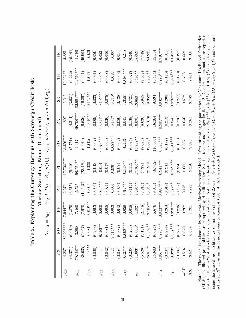
Table

5.

Expla

inin

gth

eC

urr

ency

Retu

rns

wit

hSovere

ign

Cre

dit

Ris

k:

Mark

ov

Sw

itch

ing

Model

(Conti

nued)

∆s t

+3

=β

0,ξ

t+β

1,ξ

tL

(Dt)

+β

2,ξ

tS

(Dt)

+ε t

+3,whereε t

+3i.i.d.N

(0,σ

2 ξ t)

MX

NO

PE

PH

PL

RO

ZA

SE

TH

TR

β0,0

4.23

782

.263

***

7.94

4***

2.5

76

-17.7

02***

-18.3

56***

-4.8

07

-5.6

45

16.0

52***

5.8

85

(4.3

71)

(9.9

19)

(1.8

70)

(3.6

15)

(5.1

40)

(5.7

51)

(4.2

14)

(3.6

31)

(4.2

22)

(16.1

61)

β0,1

79.1

58**

-3.3

587.

460

-5.5

27

50.7

51**

4.4

17

49.7

00***

62.5

94***

-11.7

50***

-1.1

96

(39.

635)

(5.9

57)

(7.9

70)

(12.6

27)

(23.4

29)

(9.0

72)

(9.6

36)

(16.3

67)

(2.2

91)

(46.9

04)

β1,0

-0.0

43**

*0.

081

-0.0

39***

-0.0

07

-0.0

20

-0.0

05

-0.0

49***

-0.1

52***

-0.0

17

-0.0

26

(0.0

08)

(0.2

38)

(0.0

03)

(0.0

05)

(0.0

13)

(0.0

07)

(0.0

09)

(0.0

33)

(0.0

11)

(0.0

20)

β1,1

-0.0

46-0

.183

**0.

000

0.0

84***

0.0

34

0.0

28***

-0.0

43**

-0.1

95***

0.0

05

0.0

22

(0.0

42)

(0.0

81)

(0.0

05)

(0.0

26)

(0.0

47)

(0.0

09)

(0.0

20)

(0.0

75)

(0.0

08)

(0.0

56)

β2,0

-0.0

253.

514*

**0.

003

-0.0

06

-0.2

36***

-0.0

88***

-0.1

47*

-0.2

39*

-0.0

59

-0.0

07

(0.0

54)

(0.8

87)

(0.0

12)

(0.0

28)

(0.0

71)

(0.0

32)

(0.0

80)

(0.1

28)

(0.0

48)

(0.0

51)

β2,1

0.42

7**

-0.6

69**

*0.

029

0.3

17***

0.3

18**

-0.1

12

0.0

45

1.3

56*

-0.0

86***

-0.2

15

(0.2

05)

(0.2

08)

(0.0

58)

(0.1

16)

(0.1

33)

(0.0

95)

(0.1

38)

(0.7

21)

(0.0

27)

(0.2

40)

σ0

11.0

83**

16.0

66*

4.19

2*9.2

94**

17.9

06**

15.7

37**

16.6

95*

13.8

80**

6.5

96**

15.0

89*

(5.5

20)

(9.1

31)

(2.1

78)

(3.8

16)

(7.3

71)

(7.6

26)

(8.6

20)

(5.9

45)

(2.9

47)

(7.7

48)

σ1

26.6

17*

16.5

46**

13.7

95**

15.8

40*

27.9

74

19.0

90*

24.6

70

18.3

52*

7.9

00**

24.2

25

(15.

600)

(6.6

24)

(6.6

76)

(9.0

30)

(18.7

62)

(10.8

00)

(16.3

64)

(9.5

94)

(3.4

04)

(15.1

14)

P00

0.96

1***

0.77

3***

0.93

3***

0.9

91***

0.9

41***

0.8

96***

0.9

05***

0.9

32***

0.7

73***

0.9

16***

(0.2

87)

(0.2

74)

(0.2

64)

(0.3

14)

(0.2

11)

(0.1

77)

(0.2

13)

(0.2

08)

(0.1

96)

(0.1

81)

P11

0.92

3*0.

957*

**0.

923*

**

0.9

72**

0.7

62***

0.8

11***

0.8

55

0.8

76***

0.9

24***

0.8

47**

(0.4

84)

(0.2

98)

(0.2

38)

(0.4

89)

(0.2

20)

(0.1

83)

(0.7

76)

(0.2

47)

(0.1

90)

(0.3

97)

ad.R

20.

516

0.62

00.

262

0.1

98

0.6

65

0.6

67

0.6

56

0.6

72

0.7

08

0.6

82

AIC

8.52

78.

804

7.28

17.7

29

9.2

20

9.0

20

9.2

61

8.7

39

7.4

61

9.1

05

Not

e:1.

Th

em

od

elis

esti

mat

edby

two-

stat

eM

ark

ov-S

wit

chin

gM

od

el.

Aft

eres

tim

ati

ng

the

para

met

ers

by

Maxim

um

Lik

elih

ood

Est

imati

on

(ML

E),

the

filt

ered

pro

bab

ilit

ies

are

com

pute

dby

Ham

ilto

nfi

lter

.S

eeth

ete

xt

for

mod

elsp

ecifi

cati

on

.2.

Coeffi

cien

tes

tim

ate

sare

rep

ort

edw

ith

the

New

ey-W

est

stan

dar

der

rors

inp

aren

thes

es.

Ast

eris

ks

ind

icate

sign

ifica

nce

leve

lsat

1%

(***),

5%

(**),

an

d10%

(*)

resp

ecti

vely

.3.

By

usi

ng

the

filt

ered

pro

bab

ilit

ies,

we

obta

inth

ees

tim

ate

d∆s t

+3

=[β

0,0

+β

1,0L

(Dt)+β

2,0S

(Dt)]P

0+

[β0,0

+β

1,0L

(Dt)+β

2,0S

(Dt)]P

1an

dco

mp

ute

adju

sted

R2

by

usi

ng

the

resi

du

alsu

mof

squ

ares

(RS

S).

4.

AIC

isp

rovid

ed.

30

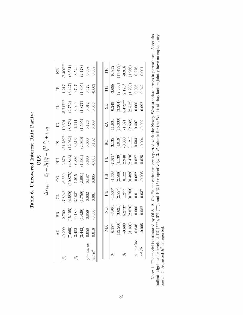
Table

6.

Unco

vere

dIn

tere

stR

ate

Pari

ty:

OL

S

∆s t

+3

=β

0+β

1(i

3 t−i3,US

t)

+ε t

+3

AU

BR

CL

CO

HU

ISID

ILJP

KR

β0

-9.2

992.

702

-7.8

94*

-6.5

50

3.6

70

-21.7

89*

10.6

91

-5.7

17**

1.2

17

-7.4

00**

(7.6

65)

(15.

105)

(4.5

89)

(10.8

75)

(4.8

43)

(12.9

62)

(8.5

73)

(2.7

52)

(3.4

27)

(3.5

61)

β1

3.48

2-0

.189

3.1

82*

1.9

15

-0.3

30

3.3

13

-1.2

14

3.0

49

0.7

47

3.5

24

(3.4

42)

(1.4

29)

(1.7

59)

(2.6

91)

(1.3

84)

(2.0

30)

(1.5

95)

(1.8

77)

(1.3

05)

(2.1

78)

p−value

0.05

80.

850

0.0

02

0.1

87

0.6

90

0.0

00

0.1

26

0.0

12

0.4

72

0.0

08

ad.R

20.

018

-0.0

060.0

61

0.0

05

-0.0

05

0.1

02

0.0

09

0.0

36

-0.0

03

0.0

38

MX

NO

PE

PH

PL

RO

ZA

SE

TH

TR

β0

6.38

7-3

.964

-4.5

63*

-1.3

68

-7.6

71*

3.1

35

11.6

34

0.2

49

-3.6

98

16.8

52

(12.

260)

(3.6

21)

(2.5

57)

(2.5

08)

(4.1

39)

(4.9

19)

(15.3

33)

(3.2

04)

(2.3

86)

(17.4

99)

β1

-0.6

005.

273*

1.2

77

0.1

22

2.9

40

-0.3

30

-1.0

21

5.4

72**

2.175*

-0.9

16

(3.1

80)

(2.8

76)

(0.7

83)

(0.4

89)

(2.4

70)

(1.1

21)

(2.6

32)

(2.5

12)

(1.2

08)

(1.9

66)

p−value

0.64

60.

000

0.0

11

0.6

82

0.0

27

0.5

03

0.4

07

0.0

00

0.0

06

0.2

76

ad.R

2-0

.005

0.08

20.0

37

-0.0

05

0.0

25

-0.0

04

-0.0

02

0.0

92

0.0

42

0.0

01

Not

e:1.

Th

em

od

elis

esti

mat

edby

OL

S.

2.C

oeffi

cien

tes

tim

ate

sare

rep

ort

edw

ith

the

New

ey-W

est

stan

dard

erro

rsin

pare

nth

eses

.A

ster

isks

ind

icat

esi

gnifi

can

cele

vels

at1%

(***

),5%

(**)

,an

d10%

(*)

resp

ecti

vely

.3.P

-valu

eis

for

the

Wald

test

that

fact

ors

join

tly

hav

en

oex

pla

nato

ryp

ower

4.A

dju

sted

R2

isre

por

ted

.

31

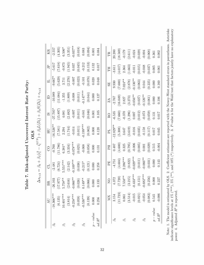
Table

7.

Ris

k-a

dju

sted

Unco

vere

dIn

tere

stR

ate

Pari

ty:

OL

S

∆s t

+3

=β

0+β

1(i

3 t−i3,US

t)

+β

2L

(Dt)

+β

3S

(Dt)

+ε t

+3

AU

BR

CL

CO

HU

ISID

ILJP

KR

β0

-18.

366*

**-2

6.10

3-2

.481

-0.7

60

-16.5

26**

-27.7

05*

-10.0

89

-9.6

67*

-5.6

17

-2.5

57

(6.1

35)

(17.

977)

(6.7

24)

(11.7

86)

(7.5

81)

(15.8

97)

(11.0

84)

(5.6

29)

(7.6

18)

(4.3

05)

β1

10.4

01**

*5.

758*

*5.5

51***

6.3

81*

2.2

94

4.0

81

-1.3

55

3.7

11

-0.8

73

6.5

06*

(3.8

14)

(2.6

16)

(2.1

42)

(3.3

34)

(1.7

44)

(2.4

82)

(1.8

09)

(2.2

76)

(1.9

45)

(3.3

51)

β2

-0.2

58**

*-0

.066

**-0

.109***

-0.0

78***

-0.0

14

-0.0

07

-0.0

08

-0.0

07

0.0

37

-0.0

37**

(0.0

59)

(0.0

26)

(0.0

38)

(0.0

25)

(0.0

11)

(0.0

11)

(0.0

11)

(0.0

23)

(0.0

45)

(0.0

18)

β3

-0.5

30**

*0.

149*

*-0

.215*

-0.0

68

-0.1

99***

-0.0

41

-0.1

47***

-0.1

01-0

.212

0.0

83

(0.1

39)

(0.0

66)

(0.1

21)

(0.0

58)

(0.0

62)

(0.0

46)

(0.0

44)

(0.0

78)

(0.1

53)

(0.0

94)

p−value

0.00

00.

000

0.0

00

0.0

00

0.0

00

0.0

01

0.0

00

0.0

20

0.1

32

0.0

01

ad.R

20.

256

0.13

30.2

58

0.1

31

0.1

20

0.1

05

0.1

27

0.0

48

0.0

17

0.0

84

MX

NO

PE

PH

PL

RO

ZA

SE

TH

TR

β0

3.15

44.

372

-4.7

51

0.4

87

-12.8

29**

-6.5

35

-2.7

67

9.9

30

-3.6

11

20.2

00

(11.

723)

(7.7

20)

(4.6

04)

(4.6

00)

(5.3

08)

(7.6

60)

(16.0

49)

(7.6

00)

(4.0

17)

(18.5

69)

β1

0.06

17.

558*

*2.2

86***

0.3

25

3.6

47

-0.3

70

2.8

27

7.0

24**

2.3

64

-0.1

79

(3.5

14)

(3.2

15)

(0.8

22)

(0.7

95)

(3.6

19)

(1.2

96)

(3.2

73)

(2.8

78)

(1.6

63)

(2.6

11)

β2

-0.0

15-0

.433

***

-0.0

29***

-0.0

06

-0.0

16

0.0

07

-0.0

56**

-0.1

36**

-0.0

11

-0.0

24

(0.0

21)

(0.1

51)

(0.0

11)

(0.0

05)

(0.0

35)

(0.0

12)

(0.0

27)

(0.0

63)

(0.0

15)

(0.0

29)

β3

-0.0

54-0

.682

***

-0.0

66**

0.0

01

-0.1

58

-0.0

73

-0.1

26**

0.0

44

-0.0

48

-0.0

04

(0.0

83)

(0.2

56)

(0.0

31)

(0.0

29)

(0.1

17)

(0.0

59)

(0.0

61)

(0.2

25)

(0.0

37)

(0.0

68)

p−value

0.54

50.

000

0.0

00

0.5

15

0.0

17

0.1

31

0.0

00

0.0

00

0.0

05

0.3

61

ad.R

2-0

.006

0.22

70.1

43

-0.0

04

0.0

45

0.0

17

0.1

06

0.1

60

0.0

61

0.0

02

Not

e:1.

Th

em

od

elis

esti

mat

edby

OL

S.

2.C

oeffi

cien

tes

tim

ate

sare

rep

ort

edw

ith

the

New

ey-W

est

stan

dard

erro

rsin

pare

nth

eses

.A

ster

isks

ind

icat

esi

gnifi

can

cele

vels

at1%

(***

),5%

(**)

,an

d10%

(*)

resp

ecti

vely

.3.P

-valu

eis

for

the

Wald

test

that

fact

ors

join

tly

hav

en

oex

pla

nato

ryp

ower

4.A

dju

sted

R2

isre

por

ted

.

32

Table 8. Explaining the Currency Returns over Different horizons:

Structural Break Model

Model 1: ∆st+m = β0 + β1D1t + εt+m

Model 2: ∆st+m = β0 + β1L(Dt) + εt+m

Model 3: ∆st+m = β0 + β1S(Dt) + εt+m

Model 4: ∆st+m = β0 + β1L(Dt) + β2S(Dt) + εt+m


m = 1

Model 1 0.075 0.025 0.151 0.054 0.043 0.245 0.158 0.024 0.031 0.180

Model 2 0.088 0.039 0.184 0.067 0.036 0.250 0.160 0.027 0.022 0.194

Model 3 0.009 0.045 0.158 0.030 0.035 0.262 0.127 0.027 0.051 0.071

Model 4 0.080 0.085 0.187 0.083 0.047 0.257 0.159 0.029 0.050 0.187

m = 3

Model 1 0.338 0.123 0.238 0.151 0.308 0.351 0.190 0.209 0.076 0.259

Model 2 0.278 0.228 0.400 0.270 0.298 0.348 0.168 0.121 0.155 0.344

Model 3 0.229 0.113 0.464 0.119 0.354 0.315 0.333 0.008 0.228 0.411

Model 4 0.601 0.239 0.551 0.326 0.345 0.344 0.368 0.011 0.215 0.469

m = 6

Model 1 0.501 0.331 0.481 0.354 0.547 0.560 0.400 0.285 0.315 0.534

Model 2 0.483 0.485 0.604 0.401 0.528 0.559 0.390 0.207 0.346 0.581

Model 3 0.297 0.317 0.540 0.320 0.519 0.420 0.308 0.279 0.364 0.536

Model 4 0.595 0.545 0.643 0.477 0.553 0.506 0.466 0.323 0.391 0.634

m = 12

Model 1 0.493 0.625 0.671 0.744 0.493 0.673 0.666 0.433 0.484 0.730

Model 2 0.506 0.705 0.649 0.663 0.471 0.659 0.568 0.452 0.535 0.712

Model 3 0.448 0.524 0.380 0.418 0.467 0.514 0.477 0.449 0.478 0.495

Model 4 0.554 0.769 0.672 0.781 0.500 0.670 0.671 0.546 0.555 0.787

Note: 1. For robustness checks, we run the same regression equations in Table 4 over different horizons(m = 1−, 3−, 6−, 12−month) and report the adjusted R2. 2. Four sets of risk factors are considered asregressors and the Bai-Perron(2003) test(with 15% trimming and 5 - 10% significance level) is applied todetect the multiple structural breaks in the regression. After identifying from zero to two breaks, structuralbreak dummy variables for each sub-period are incorporated into the regression.

33

Table 8. Explaining the Currency Returns over Different horizons:

Structural Break Model (Continued)

Model 1: ∆st+m = β0 + β1D1t + εt+m

Model 2: ∆st+m = β0 + β1L(Dt) + εt+m

Model 3: ∆st+m = β0 + β1S(Dt) + εt+m

Model 4: ∆st+m = β0 + β1L(Dt) + β2S(Dt) + εt+m


m = 1

Model 1 0.113 0.055 0.095 0.054 0.087 0.053 0.037 0.079 0.047 0.044

Model 2 0.114 0.072 0.080 0.062 0.086 0.073 0.037 0.067 0.033 0.031

Model 3 0.021 0.023 0.056 0.055 0.021 0.040 0.039 0.019 0.020 0.038

Model 4 0.108 0.059 0.082 0.059 0.083 0.075 0.054 0.087 0.048 0.036

m = 3

Model 1 0.140 0.313 0.165 0.278 0.187 0.215 0.176 0.231 0.087 0.110

Model 2 0.128 0.259 0.241 0.266 0.209 0.172 0.257 0.238 -0.004 0.015

Model 3 -0.001 0.210 0.169 0.230 0.197 0.211 0.243 0.188 0.048 0.230

Model 4 0.135 0.380 0.278 0.322 0.312 0.173 0.338 0.173 0.045 0.342

m = 6

Model 1 0.314 0.509 0.352 0.473 0.455 0.398 0.353 0.503 0.210 0.348

Model 2 0.258 0.525 0.385 0.468 0.472 0.368 0.404 0.506 0.247 0.306

Model 3 0.330 0.392 0.375 0.369 0.391 0.365 0.423 0.334 0.291 0.463

Model 4 0.366 0.624 0.444 0.545 0.471 0.417 0.497 0.511 0.270 0.578

m = 12

Model 1 0.532 0.502 0.686 0.711 0.612 0.508 0.500 0.533 0.542 0.548

Model 2 0.483 0.527 0.698 0.699 0.634 0.491 0.591 0.557 0.557 0.472

Model 3 0.437 0.409 0.617 0.535 0.564 0.424 0.460 0.288 0.390 0.453

Model 4 0.568 0.555 0.725 0.732 0.639 0.505 0.681 0.564 0.559 0.582

Note: 1. For robustness checks, we run the same regression equations in Table 4 over different horizons(m = 1−, 3−, 6−, 12−month) and report the adjusted R2. 2. Four sets of risk factors are considered asregressors and the Bai-Perron(2003) test(with 15% trimming and 5 - 10% significance level) is applied todetect the multiple structural breaks in the regression. After identifying from zero to two breaks, structuralbreak dummy variables for each sub-period are incorporated into the regression.

34

Table

9.

Expla

inin

gth

eC

urr

ency

Retu

rns

over

Diff

ere

nt

Hori

zon

s:

Mark

ov

Sw

itch

ing

Model

∆s t

+m

=β

0,ξ

t+β

1,ξ

tL

(Dt)

+β

2,ξ

tS

(Dt)

+ε t

+m,whereε t

+mi.i.d.N

(0,σ

2 ξ t)

AU

BR

CL

CO

HU

ISID

ILJP

KR

β0,0

1.38

4-1

2.97

3-5

4.97

0***

2.6

15

-8.2

34

-14.3

15*

26.0

23**

-1.1

44

1.4

70

6.3

69

(6.1

84)

(7.9

84)

(7.0

98)

(6.6

51)

(5.8

82)

(7.4

24)

(10.1

61)

(4.9

74)

(4.9

02)

(6.1

01)

β0,1

123.

417*

*82

.096

**-6

.212

53.4

20

67.1

95

2.2

01

-97.0

73***

-20.6

80-9

.244

-19.8

78

(51.

484)

(33.

780)

(6.7

42)

(35.3

13)

(61.0

63)

(32.9

53)

(24.8

42)

(12.6

19)

(8.1

54)

(18.7

78)

β1,0

-0.2

60**

*0.

008

0.84

7***

-0.0

23

-0.0

29**

0.0

13*

-0.0

77***

-0.1

12

-0.1

48

-0.1

26***

(0.0

58)

(0.0

12)

(0.0

28)

(0.0

18)

(0.0

12)

(0.0

07)

(0.0

11)

(0.0

69)

(0.1

20)

(0.0

16)

β1,1

-0.0

08-0

.115

**-0

.047*

-0.1

07

-0.0

56

-0.0

88

0.0

25*

0.0

40

0.0

30

0.1

73***

(0.1

04)

(0.0

55)

(0.0

26)

(0.0

74)

(0.0

58)

(0.0

69)

(0.0

15)

(0.0

35)

(0.0

56)

(0.0

36)

β2,0

-0.5

24**

*0.

024

-1.4

87***

-0.0

35

-0.1

67***

-0.0

53

-0.0

04

-0.2

42

-1.6

94*

-0.1

01

(0.1

91)

(0.0

77)

(0.1

56)

(0.0

90)

(0.0

56)

(0.0

48)

(0.0

52)

(0.2

08)

(0.8

64)

(0.0

92)

β2,1

2.24

3*0.

226

-0.3

83***

0.1

37

-0.2

57

-1.2

57*

-0.6

50***

-0.3

60*

0.0

64

-0.1

05

(1.3

56)

(0.1

45)

(0.1

36)

(0.2

17)

(0.2

69)

(0.7

57)

(0.1

36)

(0.2

00)

(0.2

20)

(0.3

12)

σ0

33.5

41**

31.8

95*

21.0

85

26.2

39**

33.9

93***

35.2

97***

20.8

14**

17.5

81**

24.1

15**

22.8

53**

(13.

541)

(17.

139)

(19.

498)

(11.9

74)

(12.6

61)

(13.3

49)

(8.3

59)

(7.5

99)

(11.2

21)

(11.4

08)

σ1

54.0

7867

.545

**31

.998

***

63.7

28**

89.8

80*

103.5

48

27.8

27*

37.0

67**

37.0

81**

40.2

33*

(39.

964)

(30.

734)

(11.

279)

(27.9

17)

(47.8

10)

(66.0

21)

(16.3

36)

(15.6

33)

(15.0

58)

(23.6

43)

P00

0.91

2***

0.86

3***

0.30

90.9

36***

0.9

66***

0.9

89**

0.8

53**

0.9

67***

0.9

61***

0.6

90

(0.2

86)

(0.3

29)

(0.7

90)

(0.2

77)

(0.2

90)

(0.3

89)

(0.3

38)

(0.3

43)

(0.3

51)

(0.7

06)

P11

0.30

10.

812*

*0.

977*

**

0.9

26***

0.8

42**

0.8

68*

0.3

97

0.9

64***

0.9

70***

0.3

75

(0.5

41)

(0.3

69)

(0.2

57)

(0.3

31)

(0.3

84)

(0.4

87)

(0.3

64)

(0.3

48)

(0.3

53)

(0.4

00)

ad.R

20.

493

0.21

50.

381

0.0

42

0.2

45

0.2

19

0.6

26

0.1

00

0.1

15

0.5

28

AIC

10.3

3510

.737

9.98

910.4

44

10.5

10

10.3

80

9.4

18

9.5

02

9.8

53

9.8

20

Not

e:1.

For

robu

stn

ess

chec

ks,

we

esti

mat

eth

esa

me

mod

elin

Table

5ov

erd

iffer

ent

hori

zon

s.H

ere,

esti

mati

on

resu

lts

form

=1−

month

are

rep

orte

d.

Res

ult

sfo

rm

=6−,1

2−

mon

thca

nb

ep

rovid

edu

pon

requ

est.

2.

Th

em

od

elis

esti

mate

dby

two-s

tate

Mark

ov-S

wit

chin

gM

od

el.

Aft

eres

tim

atin

gth

ep

aram

eter

sby

Max

imu

mL

ikel

ihood

Est

imati

on

(ML

E),

the

filt

ered

pro

bab

ilit

ies

are

com

pu

ted

by

Ham

ilto

nfi

lter

.3.

Coeffi

cien

tes

tim

ates

are

rep

orte

dw

ith

the

stan

dar

der

rors

inp

are

nth

eses

.A

ster

isks

ind

icate

sign

ifica

nce

leve

lsat

1%

(***),

5%

(**),

an

d10%

(*)

resp

ecti

vely

.4.

Ad

just

edR

2an

dA

ICar

ere

por

ted

.

35

Table

9.

Expla

inin

gth

eC

urr

ency

Retu

rns

over

Diff

ere

nt

Hori

zon

s:

Mark

ov

Sw

itch

ing

Model

(Conti

nued)

∆s t

+m

=β

0,ξ

t+β

1,ξ

tL

(Dt)

+β

2,ξ

tS

(Dt)

+ε t

+m,whereε t

+mi.i.d.N

(0,σ

2 ξ t)

AU

BR

CL

CO

HU

ISID

ILJP

KR

β0,0

1.38

4-1

2.97

3-5

4.97

0***

2.6

15

-8.2

34

-14.3

15*

26.0

23**

-1.1

44

1.4

70

6.3

69

(6.1

84)

(7.9

84)

(7.0

98)

(6.6

51)

(5.8

82)

(7.4

24)

(10.1

61)

(4.9

74)

(4.9

02)

(6.1

01)

β0,1

123.

417*

*82

.096

**-6

.212

53.4

20

67.1

95

2.2

01

-97.0

73***

-20.6

80-9

.244

-19.8

78

(51.

484)

(33.

780)

(6.7

42)

(35.3

13)

(61.0

63)

(32.9

53)

(24.8

42)

(12.6

19)

(8.1

54)

(18.7

78)

β1,0

-0.2

60**

*0.

008

0.84

7***

-0.0

23

-0.0

29**

0.0

13*

-0.0

77***

-0.1

12

-0.1

48

-0.1

26***

(0.0

58)

(0.0

12)

(0.0

28)

(0.0

18)

(0.0

12)

(0.0

07)

(0.0

11)

(0.0

69)

(0.1

20)

(0.0

16)

β1,1

-0.0

08-0

.115

**-0

.047*

-0.1

07

-0.0

56

-0.0

88

0.0

25*

0.0

40

0.0

30

0.1

73***

(0.1

04)

(0.0

55)

(0.0

26)

(0.0

74)

(0.0

58)

(0.0

69)

(0.0

15)

(0.0

35)

(0.0

56)

(0.0

36)

β2,0

-0.5

24**

*0.

024

-1.4

87***

-0.0

35

-0.1

67***

-0.0

53

-0.0

04

-0.2

42

-1.6

94*

-0.1

01

(0.1

91)

(0.0

77)

(0.1

56)

(0.0

90)

(0.0

56)

(0.0

48)

(0.0

52)

(0.2

08)

(0.8

64)

(0.0

92)

β2,1

2.24

3*0.

226

-0.3

83***

0.1

37

-0.2

57

-1.2

57*

-0.6

50***

-0.3

60*

0.0

64

-0.1

05

(1.3

56)

(0.1

45)

(0.1

36)

(0.2

17)

(0.2

69)

(0.7

57)

(0.1

36)

(0.2

00)

(0.2

20)

(0.3

12)

σ0

33.5

41**

31.8

95*

21.0

85

26.2

39**

33.9

93***

35.2

97***

20.8

14**

17.5

81**

24.1

15**

22.8

53**

(13.

541)

(17.

139)

(19.

498)

(11.9

74)

(12.6

61)

(13.3

49)

(8.3

59)

(7.5

99)

(11.2

21)

(11.4

08)

σ1

54.0

7867

.545

**31

.998

***

63.7

28**

89.8

80*

103.5

48

27.8

27*

37.0

67**

37.0

81**

40.2

33*

(39.

964)

(30.

734)

(11.

279)

(27.9

17)

(47.8

10)

(66.0

21)

(16.3

36)

(15.6

33)

(15.0

58)

(23.6

43)

P00

0.91

2***

0.86

3***

0.30

90.9

36***

0.9

66***

0.9

89**

0.8

53**

0.9

67***

0.9

61***

0.6

90

(0.2

86)

(0.3

29)

(0.7

90)

(0.2

77)

(0.2

90)

(0.3

89)

(0.3

38)

(0.3

43)

(0.3

51)

(0.7

06)

P11

0.30

10.

812*

*0.

977*

**

0.9

26***

0.8

42**

0.8

68*

0.3

97

0.9

64***

0.9

70***

0.3

75

(0.5

41)

(0.3

69)

(0.2

57)

(0.3

31)

(0.3

84)

(0.4

87)

(0.3

64)

(0.3

48)

(0.3

53)

(0.4

00)

ad.R

20.

493

0.21

50.

381

0.0

42

0.2

45

0.2

19

0.6

26

0.1

00

0.1

15

0.5

28

AIC

10.3

3510

.737

9.98

910.4

44

10.5

10

10.3

80

9.4

18

9.5

02

9.8

53

9.8

20

Not

e:1.

For

robu

stn

ess

chec

ks,

we

esti

mat

eth

esa

me

mod

elin

Table

5ov

erd

iffer

ent

hori

zon

s.H

ere,

esti

mati

on

resu

lts

form

=1−

month

are

rep

orte

d.

Res

ult

sfo

rm

=6−,1

2−

mon

thca

nb

ep

rovid

edu

pon

requ

est.

2.

Th

em

od

elis

esti

mate

dby

two-s

tate

Mark

ov-S

wit

chin

gM

od

el.

Aft

eres

tim

atin

gth

ep

aram

eter

sby

Max

imu

mL

ikel

ihood

Est

imati

on

(ML

E),

the

filt

ered

pro

bab

ilit

ies

are

com

pu

ted

by

Ham

ilto

nfi

lter

.3.

Coeffi

cien

tes

tim

ates

are

rep

orte

dw

ith

the

stan

dar

der

rors

inp

are

nth

eses

.A

ster

isks

ind

icate

sign

ifica

nce

leve

lsat

1%

(***),

5%

(**),

an

d10%

(*)

resp

ecti

vely

.4.

Ad

just

edR

2an

dA

ICar

ere

por

ted

.

36

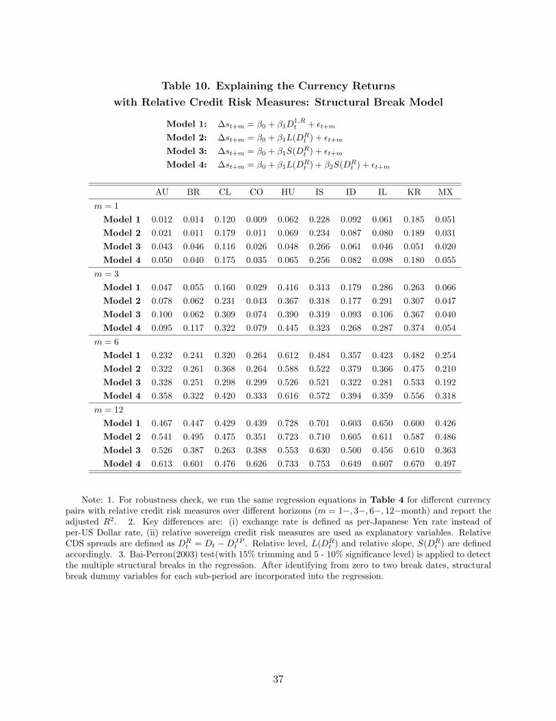
Table 10. Explaining the Currency Returns

with Relative Credit Risk Measures: Structural Break Model

Model 1: ∆st+m = β0 + β1D1,Rt + εt+m

Model 2: ∆st+m = β0 + β1L(DRt ) + εt+m

Model 3: ∆st+m = β0 + β1S(DRt ) + εt+m

Model 4: ∆st+m = β0 + β1L(DRt ) + β2S(DR

t ) + εt+m

AU BR CL CO HU IS ID IL KR MX

m = 1

Model 1 0.012 0.014 0.120 0.009 0.062 0.228 0.092 0.061 0.185 0.051

Model 2 0.021 0.011 0.179 0.011 0.069 0.234 0.087 0.080 0.189 0.031

Model 3 0.043 0.046 0.116 0.026 0.048 0.266 0.061 0.046 0.051 0.020

Model 4 0.050 0.040 0.175 0.035 0.065 0.256 0.082 0.098 0.180 0.055

m = 3

Model 1 0.047 0.055 0.160 0.029 0.416 0.313 0.179 0.286 0.263 0.066

Model 2 0.078 0.062 0.231 0.043 0.367 0.318 0.177 0.291 0.307 0.047

Model 3 0.100 0.062 0.309 0.074 0.390 0.319 0.093 0.106 0.367 0.040

Model 4 0.095 0.117 0.322 0.079 0.445 0.323 0.268 0.287 0.374 0.054

m = 6

Model 1 0.232 0.241 0.320 0.264 0.612 0.484 0.357 0.423 0.482 0.254

Model 2 0.322 0.261 0.368 0.264 0.588 0.522 0.379 0.366 0.475 0.210

Model 3 0.328 0.251 0.298 0.299 0.526 0.521 0.322 0.281 0.533 0.192

Model 4 0.358 0.322 0.420 0.333 0.616 0.572 0.394 0.359 0.556 0.318

m = 12

Model 1 0.467 0.447 0.429 0.439 0.728 0.701 0.603 0.650 0.600 0.426

Model 2 0.541 0.495 0.475 0.351 0.723 0.710 0.605 0.611 0.587 0.486

Model 3 0.526 0.387 0.263 0.388 0.553 0.630 0.500 0.456 0.610 0.363

Model 4 0.613 0.601 0.476 0.626 0.733 0.753 0.649 0.607 0.670 0.497

Note: 1. For robustness check, we run the same regression equations in Table 4 for different currencypairs with relative credit risk measures over different horizons (m = 1−, 3−, 6−, 12−month) and report theadjusted R2. 2. Key differences are: (i) exchange rate is defined as per-Japanese Yen rate instead ofper-US Dollar rate, (ii) relative sovereign credit risk measures are used as explanatory variables. RelativeCDS spreads are defined as DR

t = Dt −DJPt . Relative level, L(DR

t ) and relative slope, S(DRt ) are defined

accordingly. 3. Bai-Perron(2003) test(with 15% trimming and 5 - 10% significance level) is applied to detectthe multiple structural breaks in the regression. After identifying from zero to two break dates, structuralbreak dummy variables for each sub-period are incorporated into the regression.

37

Table 10. Explaining the Currency Returns

with Relative Credit Risk Measures: Structural Break Model (Continued)

Model 1: ∆st+m = β0 + β1D1,Rt + εt+m

Model 2: ∆st+m = β0 + β1L(DRt ) + εt+m

Model 3: ∆st+m = β0 + β1S(DRt ) + εt+m

Model 4: ∆st+m = β0 + β1L(DRt ) + β2S(DR

t ) + εt+m

NO PE PH PL RO ZA SE TH TR US

m = 1

Model 1 0.028 0.055 0.009 0.084 0.067 0.029 0.021 0.071 0.007 0.112

Model 2 0.025 0.053 0.020 0.096 0.106 0.022 0.018 0.064 0.003 0.082

Model 3 0.006 0.034 0.010 0.024 0.059 0.023 0.012 0.032 0.029 0.036

Model 4 0.015 0.069 0.024 0.091 0.136 0.022 0.026 0.056 0.023 0.074

m = 3

Model 1 0.103 0.192 0.081 0.256 0.243 0.050 0.046 0.137 0.004 0.129

Model 2 0.144 0.144 0.132 0.238 0.251 0.027 0.018 0.236 0.096 0.116

Model 3 0.190 0.006 0.107 0.205 0.212 0.262 0.267 0.209 0.362 0.118

Model 4 0.211 0.143 0.157 0.298 0.287 0.325 0.255 0.266 0.364 0.110

m = 6

Model 1 0.244 0.316 0.269 0.448 0.448 0.368 0.254 0.295 0.274 0.349

Model 2 0.129 0.256 0.239 0.443 0.446 0.337 0.278 0.289 0.240 0.395

Model 3 0.294 0.237 0.297 0.338 0.367 0.416 0.347 0.325 0.520 0.444

Model 4 0.350 0.369 0.337 0.470 0.491 0.438 0.421 0.320 0.520 0.438

m = 12

Model 1 0.376 0.369 0.397 0.635 0.658 0.382 0.416 0.398 0.378 0.679

Model 2 0.386 0.421 0.379 0.604 0.659 0.397 0.480 0.398 0.358 0.690

Model 3 0.386 0.569 0.486 0.510 0.556 0.307 0.421 0.406 0.376 0.689

Model 4 0.520 0.595 0.508 0.646 0.721 0.497 0.520 0.405 0.398 0.694

Note: 1. For robustness check, we run the same regression equations in Table 4 for different currencypairs with relative credit risk measures over different horizons (m = 1−, 3−, 6−, 12−month) and report theadjusted R2. 2. Key differences are: (i) exchange rate is defined as per-Japanese Yen rate instead ofper-US Dollar rate, (ii) relative sovereign credit risk measures are used as explanatory variables. RelativeCDS spreads are defined as DR

t = Dt −DJPt . Relative level, L(DR

t ) and relative slope, S(DRt ) are defined

accordingly. 3. Bai-Perron(2003) test(with 15% trimming and 5 - 10% significance level) is applied to detectthe multiple structural breaks in the regression. After identifying from zero to two break dates, structuralbreak dummy variables for each sub-period are incorporated into the regression.

38

Table

11.

Expla

inin

gth

eC

urr

ency

Retu

rns

wit

hR

ela

tive

Cre

dit

Ris

kM

easu

res:

Mark

ov

Sw

itch

ing

Model

∆s t

+3

=β

0,ξ

t+β

1,ξ

tL

(DR t

)+β

2,ξ

tS

(DR t

)+ε t

+3,whereε t

+3i.i.d.N

(0,σ

2 ξ t)

AU

BR

CL

CO

HU

ISID

ILK

RM

X

β0,0

-1.5

00-3

.884

194.

793***

12.1

64*

-1.1

44

-10.1

59

8.9

77

-4.5

38

-7.0

48*

7.0

13

(5.1

50)

(6.2

56)

(4.7

70)

(6.5

77)

(4.2

59)

(82.6

34)

(5.5

22)

(5.8

52)

(4.0

61)

(8.2

41)

β0,1

145.

383*

**51

.372

*-1

.544

-18.6

30

121.1

21***

-42.6

05

69.9

80**

8.5

73

16.9

98

61.8

39

(35.

944)

(27.

257)

(5.6

65)

(23.5

89)

(31.5

44)

(14246)

(32.4

06)

(13.6

92)

(14.8

73)

(56.4

84)

β1,0

-0.1

08-0

.016

-0.2

40***

-0.0

73***

-0.0

34***

0.0

16

-0.0

32***

-0.0

28

0.0

25

-0.0

24

(0.1

64)

(0.0

12)

(0.0

15)

(0.0

19)

(0.0

09)

(0.0

75)

(0.0

12)

(0.0

19)

(0.0

18)

(0.0

27)

β1,1

-1.2

710.

026

-0.0

42

0.1

34

-0.1

14***

-0.0

61

-0.1

56***

0.0

25

-0.0

16

0.0

18

(1.8

27)

(0.0

56)

(0.0

44)

(0.0

88)

(0.0

29)

(2.3

47)

(0.0

14)

(0.0

90)

(0.0

49)

(0.0

53)

β2,0

0.26

40.

041

0.71

8***

-0.0

14

-0.0

63

0.0

04

0.0

00

0.0

48

0.1

07

0.1

08

(0.5

61)

(0.0

76)

(0.2

09)

(0.0

64)

(0.0

49)

(0.3

89)

(0.0

03)

(0.1

51)

(0.0

88)

(0.1

07)

β2,1

0.41

0-0

.472

*-0

.216

-0.1

58

-0.0

14

-1.0

67

-0.6

85***

0.0

81

-0.0

32

0.1

45

(5.6

70)

(0.2

65)

(0.1

94)

(0.3

35)

(0.0

87)

(68.8

13)

(0.1

63)

(0.3

32)

(0.3

18)

(0.4

21)

σ0

22.6

21**

24.3

17**

0.25

7*

17.9

10**

21.4

85**

21.2

84

21.8

35***

11.0

52

10.8

48**

24.0

80**

(9.7

72)

(9.9

60)

(0.1

50)

(7.2

86)

(8.9

43)

(20.9

40)

(8.4

43)

(6.7

01)

(4.8

96)

(10.2

01)

σ1

39.4

2144

.554

23.7

03**

44.9

76*

34.2

37**

102.4

25

24.9

80**

35.1

77*

42.9

80

45.2

27

(38.

186)

(30.

309)

(9.3

02)

(24.4

45)

(15.2

73)

(1047)

(11.1

32)

(19.2

74)

(31.0

69)

(36.6

21)

P00

0.99

3***

0.95

7***

0.404

0.9

02***

0.9

76***

0.9

89

0.9

93***

0.9

05**

*0.9

27***

0.9

71***

(0.3

52)

(0.2

37)

(0.7

36)

(0.2

08)

(0.2

37)

(8.8

72)

(0.3

59)

(0.2

34)

(0.2

40)

(0.2

42)

P11

0.88

80.

789*

**0.

991***

0.7

93***

0.8

62**

0.8

98

0.8

17*

0.8

96***

0.8

65**

0.8

18**

(0.8

30)

(0.2

93)

(0.3

08)

(0.2

09)

(0.3

52)

(11.9

33)

(0.4

78)

(0.2

63)

(0.3

91)

(0.3

52)

ad.R

20.

533

0.56

70.

441

0.3

29

0.5

76

0.1

39

0.4

53

0.0

92

0.2

48

0.4

44

AIC

9.28

49.

782

9.181

9.6

11

9.4

18

9.5

14

9.1

87

9.1

25

8.9

93

9.6

00

Not

e:1.

For

rob

ust

nes

sch

ecks,

we

esti

mat

eth

esa

me

mod

elin

Table

5fo

rd

iffer

ent

curr

ency

pair

sw

ith

rela

tive

cred

itri

skm

easu

res

over

diff

eren

th

oriz

ons

(m=

1−,3−,6−,1

2−

mon

th):

(i)

exch

an

ge

rate

isd

efin

edas

per

-Japan

ese

Yen

rate

sin

stea

dof

per

-US

Doll

ar

rate

s,(i

i)re

lati

veso

vere

ign

cred

itri

skm

easu

res

are

use

das

exp

lan

ato

ryva

riab

les.

Rel

ati

ve

CD

Ssp

read

sare

defi

ned

asDR t

=Dt−DJP

t.

Rel

ati

vele

vel,L

(DR t

)an

dre

lati

vesl

ope,S

(DR t

)ar

edefi

ned

acco

rdin

gly.

2.

Her

e,es

tim

ati

on

resu

lts

form

=3−

month

are

rep

ort

ed.

Res

ult

sfo

rm

=1−,6−,1

2−

month

can

be

pro

vid

edu

pon

requ

est.

39

Table

11.

Expla

inin

gth

eC

urr

ency

Retu

rns

wit

hR

ela

tive

Cre

dit

Ris

kM

easu

res:

Mark

ov

Sw

itch

ing

Model

(Conti

nued)

∆s t

+3

=β

0,ξ

t+β

1,ξ

tL

(DR t

)+β

2,ξ

tS

(DR t

)+ε t

+3,whereε t

+3i.i.d.N

(0,σ

2 ξ t)

NO

PE

PH

PL

RO

ZA

SE

TH

TR

US

β0,0

162.

424*

**10

.026

**-1

.182

-5.6

46

-7.8

53

5.2

97

-4.6

85

-29.8

25***

36.2

54***

-4.1

23

(3.1

82)

(4.1

19)

(14.

992)

(6.1

47)

(6.4

81)

(9.4

48)

(4.3

44)

(8.4

68)

(9.7

66)

(2.7

36)

β0,1

-1.6

46-5

3.18

1***

5.53

251.2

85

23.0

95

80.8

58**

59.8

02

6.6

74

-142.8

00***

7.9

19

(3.9

97)

(15.

157)

(67.

009)

(87.8

71)

(14.3

30)

(39.4

88)

(36.4

39)

(8.3

26)

(20.9

44)

(6.7

93)

β1,0

1.01

0***

-0.0

030.

005

-0.0

63***

-0.0

02

-0.0

77***

0.0

58

0.2

68***

-0.0

70***

-0.0

43

(0.0

38)

(0.0

20)

(0.0

18)

(0.0

23)

(0.0

09)

(0.0

29)

(0.0

75)

(0.0

51)

(0.0

18)

(0.0

48)

β1,1

-0.0

050.

053

0.00

90.0

18

0.0

57*

-0.0

95

-0.0

15

-0.0

51***

0.1

75***

0.1

30

(0.0

54)

(0.0

54)

(0.1

19)

(0.2

37)

(0.0

31)

(0.0

62)

(0.0

66)

(0.0

18)

(0.0

21)

(0.0

85)

β2,0

-1.7

95**

*0.

119*

0.08

10.0

94

0.0

66

-0.0

92

-0.0

69

0.1

24

0.0

50

-0.1

57**

(0.1

78)

(0.0

62)

(0.1

23)

(0.1

64)

(0.0

74)

(0.0

75)

(0.2

25)

(0.1

46)

(0.0

56)

(0.0

78)

β2,1

-0.0

46-0

.555

**-0

.253

0.1

04

0.0

69

-0.0

98

1.5

59*

-0.1

26

-0.9

22***

-0.0

42

(0.2

74)

(0.2

25)

(0.7

48)

(0.4

45)

(0.2

06)

(0.2

76)

(0.9

06)

(0.1

05)

(0.0

74)

(0.2

52)

σ0

5.68

012

.532

**18

.654

18.3

52

18.8

25**

22.7

99**

18.2

89**

20.8

76*

24.9

01**

7.9

25

(5.1

65)

(5.0

45)

(12.

014)

(13.0

08)

(7.9

13)

(9.5

18)

(8.8

78)

(12.5

80)

(11.5

05)

(5.1

42)

σ1

23.6

82**

34.5

0521

.708

43.6

76

31.3

02

39.2

92

36.4

77*

11.6

32

25.3

85

26.3

69**

(9.3

93)

(21.

867)

(13.

470)

(37.7

54)

(21.4

72)

(27.7

66)

(19.8

14)

(7.4

29)

(16.0

61)

(11.7

43)

P00

0.59

00.

956*

**0.

972

0.9

50**

0.9

24***

0.9

58***

0.9

44***

0.8

80***

0.9

57***

0.7

95***

(0.4

64)

(0.2

47)

(1.3

35)

(0.4

12)

(0.1

75)

(0.2

71)

(0.2

42)

(0.2

62)

(0.2

80)

(0.2

12)

P11

0.96

1***

0.86

0***

0.89

50.8

11***

0.8

22***

0.8

05***

0.8

27***

0.8

45***

0.7

44**

0.8

74***

(0.1

71)

(0.2

71)

(0.9

03)

(0.3

05)

(0.2

17)

(0.2

75)

(0.2

59)

(0.2

25)

(0.3

73)

(0.2

77)

ad.R

20.

500

0.16

20.

394

0.5

92

0.5

67

0.5

83

0.4

97

0.4

64

0.5

67

0.0

66

AIC

9.30

28.

683

8.96

69.4

39

9.4

81

9.6

49

9.4

03

8.7

97

9.6

03

8.9

02

Not

e:1.

For

rob

ust

nes

sch

ecks,

we

esti

mat

eth

esa

me

mod

elin

Table

5fo

rd

iffer

ent

curr

ency

pair

sw

ith

rela

tive

cred

itri

skm

easu

res

over

diff

eren

th

oriz

ons

(m=

1−,3−,6−,1

2−

mon

th):

(i)

exch

an

ge

rate

isd

efin

edas

per

-Japan

ese

Yen

rate

sin

stea

dof

per

-US

Doll

ar

rate

s,(i

i)re

lati

veso

vere

ign

cred

itri

skm

easu

res

are

use

das

exp

lan

ato

ryva

riab

les.

Rel

ati

veC

DS

spre

ad

sare

defi

ned

asDR t

=Dt−DJP

t.

Rel

ati

vele

vel,L

(DR t

an

dre

lati

vesl

ope,S

(DR t

are

defi

ned

acco

rdin

gly.

2.H

ere,

esti

mati

on

resu

lts

form

=3−

month

are

rep

ort

ed.

Res

ult

sfo

rm

=1−,6−,1

2−

month

can

be

pro

vid

edu

pon

reques

t.

40

Figure 1: Exchange Rate Change

(Annualized %; Home Currency/USD)

Note: 1. Figure 1 shows the quarterly change of exchange rate, ∆st+3 = st+3 − st, where st is thelogged home currency price per USD. 2. Sample period is from January, 2004 to June, 2017. All rates arein annualized percentage points.

41

Figure 1: Exchange Rate Change (Continued)

(Annualized %; Home Currency/USD)

Note: 1. Figure 1 shows the quarterly change of exchange rate, ∆st+3 = st+3 − st, where st is thelogged home currency price per USD. 2. Sample period is from January, 2004 to June, 2017. All rates arein annualized percentage points.

42

Figure 2: Sovereign Credit Default Swap

(Basis Point)

Note: 1. Figure 2 shows sovereign credit default swap (CDS) spreads of 1, 2, 3, 5, 7, 10 years tenor:Red for 1 year, Cyan for 2 year, Green for 3 year, Black for 5 year, Magenta for 7 year and Blue for 10 yeartenor CDS spread. 2. Sample period is from January, 2004 to June, 2017, but shorter for some countries.All values are in annuity basis points.

43

Figure 2: Sovereign Credit Default Swap (Continued)

(Basis Point)

Note: 1. Figure 2 shows sovereign credit default swap (CDS) spreads of 1, 2, 3, 5, 7, 10 years tenor:Red for 1 year, Cyan for 2 year, Green for 3 year, Black for 5 year, Magenta for 7 year and Blue for 10 yeartenor CDS spread. 2. Sample period is from January, 2004 to June, 2017, but shorter for some countries.All values are in annuity basis points.

44

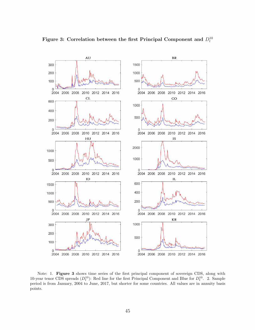
Figure 3: Correlation between the first Principal Component and D10t

Note: 1. Figure 3 shows time series of the first principal component of sovereign CDS, along with10-year tenor CDS spreads (D10

t ): Red line for the first Principal Component and Blue for D10t . 2. Sample

period is from January, 2004 to June, 2017, but shorter for some countries. All values are in annuity basispoints.

45

Figure 3: Correlation between the first Principal Component and D10t

(Continued)

Note: 1. Figure 3 shows time series of the first principal component of sovereign CDS, along with10-year tenor CDS spreads (D10

t ): Red line for the first Principal Component and Blue for D10t . 2. Sample

period is from January, 2004 to June, 2017, but shorter for some countries. All values are in annuity basispoints.

46

Figure 4: Correlation between the second Principal Component and D1t −D10

t

Note: 1. Figure 4 shows time series of the second principal component of sovereign CDS, along withthe difference between 1-year and 10-year tenor CDS spreads (D1

t −D10T ): Red line for the second Principal

Component and Blue for D1t −D10

t . Positive value implies an inverted CDS curve. 2. Sample period is fromJanuary, 2004 to June, 2017, but shorter for some countries. All values are in annuity basis points.

47

Figure 4: Correlation between the second Principal Component and D1t −D10

t

(Continued)

Note: 1. Figure 4 shows time series of the second principal component of sovereign CDS, along withthe difference between 1-year and 10-year tenor CDS spreads (D1

t −D10T ): Red line for the second Principal

Component and Blue for D1t −D10

t . Positive value implies an inverted CDS curve. 2. Sample period is fromJanuary, 2004 to June, 2017, but shorter for some countries. All values are in annuity basis points.

48

Figure 5: Probability in State 1

Note: 1. Figure 5 shows the filtered probability in state 1 from Markov-Switching model estimation:∆st+3 = β0,ξt + β1,ξtL(Dt) + β2,ξtS(Dt) + εt+3, where εt+3 i.i.d.N(0, σ2

ξt). State 1 represents “high volatil-

ity”state. 2. Dark shades show the months when VIX index is greater than 25 and light shades show themonths when VIX index is between 20 and 25.

49

Figure 5: Probability in State 1 (Continued)

Note: 1. Figure 5 shows the filtered probability in state 1 from Markov-Switching model estimation:∆st+3 = β0,ξt + β1,ξtL(Dt) + β2,ξtS(Dt) + εt+3, where εt+3 i.i.d.N(0, σ2

ξt). State 1 represents “high volatil-

ity”state. 2. Dark shades show the months when VIX index is greater than 25 and light shades show themonths when VIX index is between 20 and 25.

50

Figure 6: Comparing the Adjusted R2 over 36-month Rolling Windows:

Level or Slope?

Note: 1. Figure 6 compares the goodness of fit measures (adjusted R2) over 36-month rolling windowsfrom two models: 1) Level-only model: ∆st+3 = β0 + β1L(Dt) + εt+3; 2) Slope-only model: ∆st+3 =β0 + β1S(Dt) + εt+3. 2. Blue line represents adjusted R2s from level-only model and Red line showsadjusted R2s from slope-only model. Gray bar graph shows the difference in adjusted R2s from two modelsdefined as “adjusted R2 from slope-only model − adjusted R2 from level-only model”. If the difference ispositive, slope-model explains relatively more than level-only model for that regression window. 3. X-axisrepresents the midpoint of each window.

51

Figure 6: Comparing the Adjusted R2 over 36-month Rolling Window:

Level or Slope? (Continued)

Note: 1. Figure 6 compares the goodness of fit measures (adjusted R2) over 36-month rolling windowsfrom two models: 1) Level-only model: ∆st+3 = β0 + β1L(Dt) + εt+3; 2) Slope-only model: ∆st+3 =β0 + β1S(Dt) + εt+3. 2. Blue line represents adjusted R2s from level-only model and Red line showsadjusted R2s from slope-only model. Gray bar graph shows the difference in adjusted R2s from two modelsdefined as “adjusted R2 from slope-only model − adjusted R2 from level-only model”. If the difference ispositive, slope-model explains relatively more than level-only model for that regression window. 3. X-axisrepresents the midpoint of each window.

52

Figure 7: Comparing the P − values over 36-month Rolling Windows:

Level or Slope?

Note: 1. Figure 7 compares the statistical significance (P − value) over 36-month rolling windows oflevel and slope factors. From the regression of ∆st+3 = β0 +β1L(Dt)+β1S(Dt)+εt+3, we obtain P −valuesfor level and slope factors. If P − value ≤ 0.01, we give “3”. If 0.01 < P − value ≤ 0.05, we give “2”. If0.05 < P − value ≤ 0.1, we give “1”. Otherwise, “0”. 2. Blue line for level factor and Red line for slopefactor. 3. X-axis represents the midpoint of each window.

53


Level or Slope? (Continued)

Note: 1. Figure 7 compares the statistical significance (P − value) over 36-month rolling windows oflevel and slope factors. From the regression of ∆st+3 = β0 +β1L(Dt)+β1S(Dt)+εt+3, we obtain P −valuesfor level and slope factors. If P − value ≤ 0.01, we give “3”. If 0.01 < P − value ≤ 0.05, we give “2”. If0.05 < P − value ≤ 0.1, we give “1”. Otherwise, “0”. 2. Blue line for level factor and Red line for slopefactor. 3. X-axis represents the midpoint of each window.

54

Figure 8: Comparing the Adjusted R2 over 36-month Rolling Windows:

Relative Level or Relative Slope?

Note: 1. Figure 8 is the robustness check for Figure 6: 1) Relative Level-only model: ∆st+m =β0 + β1L(DR

t ) + εt+m; 2) Slope-only model: ∆st+m = β0 + β1S(DRt ) + εt+m. Here, we show the results

from JPY as denominating currency, with relative risk measures as regressors, and for m = 6−month. Theresults from USD and/or over different horizons (m = 1−, 3−, 12−month) can be provided upon request.2. Blue line: adjusted R2 from level-only model, Red line: adjusted R2 from slope-only model. Gray bar:adjusted R2 from slope-only model − adjusted R2 from level-only model.

55

Figure 8: Comparing the Adjusted R2 over 36-month Rolling Window:

Relative Level or Relative Slope? (Continued)

Note: 1. Figure 8 is the robustness check for Figure 6: 1) Relative Level-only model: ∆st+m =β0 + β1L(DR

t ) + εt+m; 2) Slope-only model: ∆st+m = β0 + β1S(DRt ) + εt+m. Here, we show the results

from JPY as denominating currency, with relative risk measures as regressors, and for m = 6−month. Theresults from USD and/or over different horizons (m = 1−, 3−, 12−month) can be provided upon request.2. Blue line: adjusted R2 from level-only model, Red line: adjusted R2 from slope-only model. Gray bar:adjusted R2 from slope-only model − adjusted R2 from level-only model.

56


Relative Level or Relative Slope?

Note: 1. Figure 9 is the robustness check for Figure 7. From the regression of ∆st+m = β0 +β1L(DR

t ) + β1S(DRt ) + εt+m, we obtain P − values for level and slope factors. If P − value ≤ 0.01, we give

“3”. If 0.01 < P − value ≤ 0.05, we give “2”. If 0.05 < P − value ≤ 0.1, we give “1”. Otherwise, “0”.Here, we show the results from JPY as denominating currency, with relative risk measures as regressors, andfor m = 6−month. The results from USD and/or over different horizons (m = 1−, 3−, 12−month) can beprovided upon request. 2. Blue line for level factor and Red line for slope factor.

57


Relative Level or Relative Slope? (Continued)

Note: 1. Figure 9 is the robustness check for Figure 7. From the regression of ∆st+m = β0 +β1L(DR

t ) + β1S(DRt ) + εt+m, we obtain P − values for level and slope factors. If P − value ≤ 0.01, we give

“3”. If 0.01 < P − value ≤ 0.05, we give “2”. If 0.05 < P − value ≤ 0.1, we give “1”. Otherwise, “0”.Here, we show the results from JPY as denominating currency, with relative risk measures as regressors, andfor m = 6−month. The results from USD and/or over different horizons (m = 1−, 3−, 12−month) can beprovided upon request. 2. Blue line for level factor and Red line for slope factor.

58

Appendix

What is Sovereign Credit Default Swap?

Sovereign Credit Default Swap (CDS) is a bilateral Over-the-Counter(OTC) agreement

in which protection buyer purchases insurance against contingent credit events by paying

an annuity premium quarterly or bi-annually and protection seller compensates for the loss

given credit events. Protection buyers are usually banks, security firms and hedge funds

and protection sellers are mostly insurance companies and banks. In practice, there is

no default in government bond. Instead, International Swap and Derivative Association

(ISDA) references four types of credit events: acceleration, failure to pay, restructuring, and

repudiation.

There are three types of cash flows associated with CDS contract. 1) If there is no credit

event until the end of the contract, only protection buyer pays an annuity premium for the

contract tenor. The protection seller pays nothing. 2) If one of the credit events is triggered

prior to the tenor, the buyer pays an annuity premium until the credit event happens and the

contract terminates. The seller compensates the buyer for its loss given a credit event. There

are two types of settlement. In the physical settlement, the buyer provides the seller the

deliverable obligations of the reference entity and the seller pays the buyer a cash payment

amounting to its full aggregate notional amount. In cash settlement, the seller pays the buyer

a cash payment amounting to a full in market value of a debt obligation of the reference

entity. 3) Each counter party of CDS contract can unwind the contract prior to the tenor.

In order to unwind the contract, they need to agree on early termination or assignment to

another counter party or they can offset the transaction in the market. In any case, they

need to pay or receive the Mark-to-Market value, which is the present value of difference

in annuity payment over remaining contract period. For example, if the CDS tightens, the

buyer needs to pay the Mark-to-Market value to seller.

Sovereign CDS has been increasing in use from early 2000s. According to the Bank for

International Settlement (BIS) statistics, sovereign CDS exploded from 6.4 trillion dollars

in 2004 to a peak of 58.2 trillion dollars in 2007. The amount has since come down because

the credit derivatives were central to the 2007-2009 financial crisis.

Sovereign CDS: Outstanding notional amount (billion USD)

2004 2005 2006 2007 2008 2009 2010 2011 2012 2013 2014 2015 2016

6396 13908 28650 58244 41883 32693 29898 28626 25068 21020 16399 12294 9857

Note: 1. Each number represents the gross notional amount outstanding in the second half of each year.

2. source: www.bis.org

59

While corporate CDS is mostly concentrated around five-year contracts, sovereign CDS

is well diversified over different tenors. Based on the BIS statistics, we compute market shares

of each tenor contract from 2004 to 2016. The total volume of notional amount outstanding

with tenor less than one year consist 12.01%, with tenor between two to five years 67.10%

and with tenor over five years 20.88%. The interesting feature is that after 2011, short tenors

have gradually been trading more relative to long tenors.

Market of sovereign CDS over different tenors (% in volume)

Note: 1. Market share is computed as total volume of notional amount outstanding of each tenor group

compared that of all tenors. 2. source: www.bis.org

60

Appendix Tables

Table A1. Explaining the Excess Currency Returns

with Sovereign Credit Risk: Structural Break Model


Model 1: xrt+3 = β0 + β1D1t + εt+3

p− value 0.000 0.006 0.000 0.002 0.005 0.000 0.000 0.032 0.033 0.000

ad.R2 0.126 0.059 0.176 0.098 0.086 0.244 0.176 0.055 0.056 0.192

Model 2: xrt+3 = β0 + β1L(Dt) + εt+3

p− value 0.000 0.002 0.000 0.000 0.004 0.000 0.000 0.007 0.027 0.000

ad.R2 0.131 0.074 0.217 0.147 0.093 0.250 0.186 0.081 0.060 0.212

Model 3: xrt+3 = β0 + β1S(Dt) + εt+3

p− value 0.003 0.002 0.000 0.011 0.002 0.000 0.000 0.030 0.014 0.003

ad.R2 0.100 0.075 0.180 0.074 0.100 0.280 0.221 0.056 0.071 0.097

Model 4: xrt+3 = β0 + β1L(Dt) + β2S(Dt) + εt+3

p− value 0.000 0.000 0.000 0.000 0.011 0.000 0.000 0.003 0.052 0.000

ad.R2 0.245 0.127 0.212 0.149 0.087 0.273 0.230 0.111 0.058 0.199


Model 1: xrt+3 = β0 + β1D1t + εt+3

p− value 0.000 0.010 0.000 0.000 0.002 0.001 0.019 0.013 0.008 0.004

ad.R2 0.164 0.092 0.130 0.101 0.102 0.108 0.067 0.086 0.070 0.085

Model 2: xrt+3 = β0 + β1L(Dt) + εt+3

p− value 0.000 0.013 0.000 0.000 0.001 0.001 0.007 0.018 0.003 0.005

ad.R2 0.167 0.087 0.137 0.110 0.111 0.112 0.083 0.081 0.085 0.081

Model 3: xrt+3 = β0 + β1S(Dt) + εt+3

p− value 0.007 0.046 0.012 0.000 0.033 0.000 0.013 0.043 0.086 0.000

ad.R2 0.085 0.062 0.068 0.097 0.056 0.133 0.073 0.063 0.030 0.124

Model 4: xrt+3 = β0 + β1L(Dt) + β2S(Dt) + εt+3

p− value 0.000 0.015 0.000 0.000 0.001 0.001 0.001 0.015 0.008 0.000

ad.R2 0.161 0.099 0.143 0.160 0.125 0.134 0.123 0.098 0.084 0.200

Note: 1. This table is Appendix to Table 4. Instead of regressing quarterly exchange rate changes, weregress quarterly excess currency returns (xrt+3 = i3t − i

3,USt −∆st+3) on four different sets of risk factors

and then apply the Bai-Perron(2003) test(with 15% trimming and 5 - 10% significance level) to detect themultiple structural breaks in the regression. Zero to two breaks are detected. 2. After identifying thebreak dates, structural break dummy variables for each sub-period are incorporated into the regression. 3.P -value is for the Wald test that factors jointly have no explanatory power 4. Adjusted R2 is reported.

61

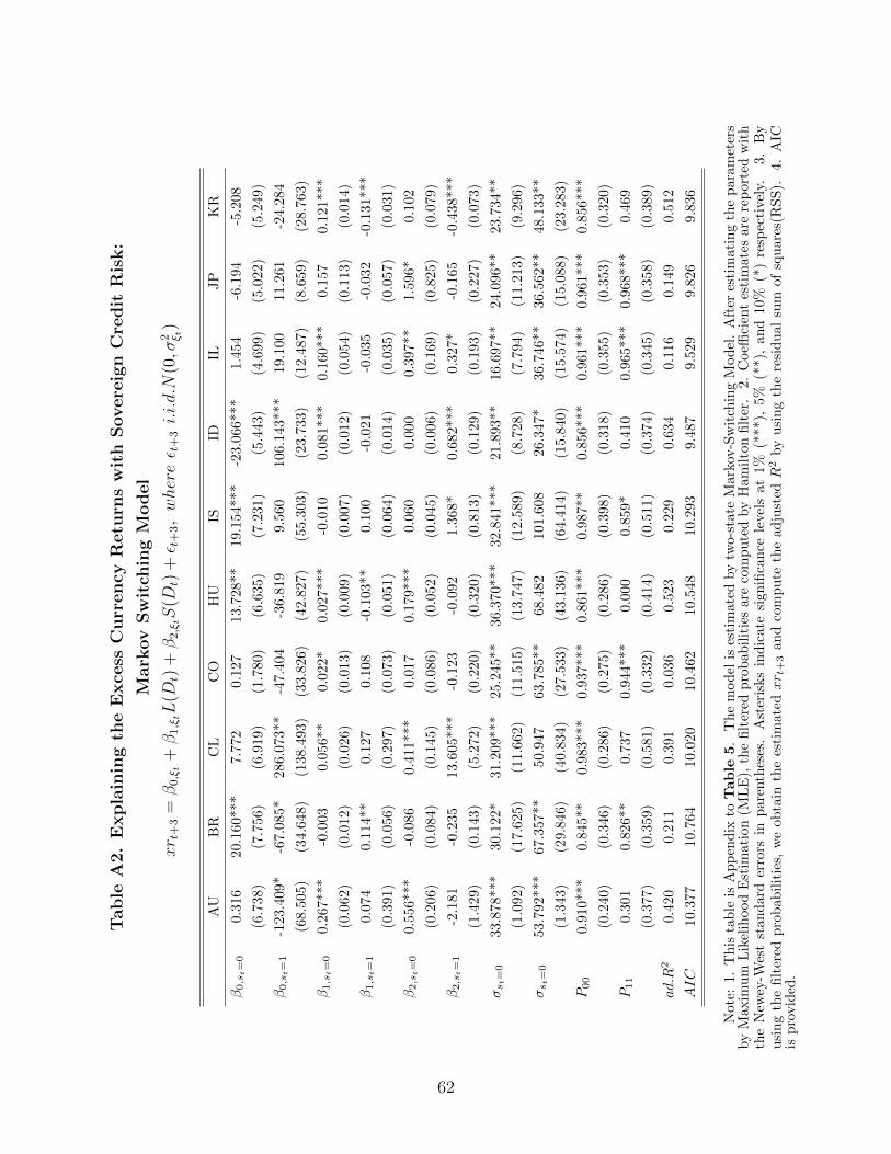
Table

A2.

Expla

inin

gth

eE

xce

ssC

urr

ency

Retu

rns

wit

hSovere

ign

Cre

dit

Ris

k:

Mark

ov

Sw

itch

ing

Model

xr t

+3

=β

0,ξ

t+β

1,ξ

tL

(Dt)

+β

2,ξ

tS

(Dt)

+ε t

+3,whereε t

+3i.i.d.N

(0,σ

2 ξ t)

AU

BR

CL

CO

HU

ISID

ILJP

KR

β0,s

t=

00.

316

20.1

60**

*7.

772

0.1

27

13.7

28**

19.1

54***

-23.0

66***

1.4

54

-6.1

94

-5.2

08

(6.7

38)

(7.7

56)

(6.9

19)

(1.7

80)

(6.6

35)

(7.2

31)

(5.4

43)

(4.6

99)

(5.0

22)

(5.2

49)

β0,s

t=

1-1

23.4

09*

-67.

085*

286.

073**

-47.4

04

-36.8

19

9.5

60

106.1

43***

19.1

0011.2

61

-24.2

84

(68.

505)

(34.

648)

(138

.493)

(33.8

26)

(42.8

27)

(55.3

03)

(23.7

33)

(12.4

87)

(8.6

59)

(28.7

63)

β1,s

t=

00.

267*

**-0

.003

0.05

6**

0.0

22*

0.0

27***

-0.0

10

0.0

81***

0.1

60**

*0.1

57

0.1

21***

(0.0

62)

(0.0

12)

(0.0

26)

(0.0

13)

(0.0

09)

(0.0

07)

(0.0

12)

(0.0

54)

(0.1

13)

(0.0

14)

β1,s

t=

10.

074

0.11

4**

0.127

0.1

08

-0.1

03**

0.1

00

-0.0

21

-0.0

35-0

.032

-0.1

31***

(0.3

91)

(0.0

56)

(0.2

97)

(0.0

73)

(0.0

51)

(0.0

64)

(0.0

14)

(0.0

35)

(0.0

57)

(0.0

31)

β2,s

t=

00.

556*

**-0

.086

0.41

1***

0.0

17

0.1

79***

0.0

60

0.0

00

0.3

97**

1.5

96*

0.1

02

(0.2

06)

(0.0

84)

(0.1

45)

(0.0

86)

(0.0

52)

(0.0

45)

(0.0

06)

(0.1

69)

(0.8

25)

(0.0

79)

β2,s

t=

1-2

.181

-0.2

3513

.605***

-0.1

23

-0.0

92

1.3

68*

0.6

82***

0.3

27*

-0.1

65

-0.4

38***

(1.4

29)

(0.1

43)

(5.2

72)

(0.2

20)

(0.3

20)

(0.8

13)

(0.1

29)

(0.1

93)

(0.2

27)

(0.0

73)

σst=

033

.878

***

30.1

22*

31.2

09***

25.2

45**

36.3

70***

32.8

41***

21.8

93**

16.6

97**

24.0

96**

23.7

34**

(1.0

92)

(17.

625)

(11.

662)

(11.5

15)

(13.7

47)

(12.5

89)

(8.7

28)

(7.7

94)

(11.2

13)

(9.2

96)

σst=

053

.792

***

67.3

57**

50.9

47

63.7

85**

68.4

82

101.6

08

26.3

47*

36.7

46**

36.5

62**

48.1

33**

(1.3

43)

(29.

846)

(40.

834)

(27.5

33)

(43.1

36)

(64.4

14)

(15.8

40)

(15.5

74)

(15.0

88)

(23.2

83)

P00

0.91

0***

0.84

5**

0.98

3***

0.9

37***

0.8

61***

0.9

87**

0.8

56***

0.9

61**

*0.9

61***

0.8

56***

(0.2

40)

(0.3

46)

(0.2

86)

(0.2

75)

(0.2

86)

(0.3

98)

(0.3

18)

(0.3

55)

(0.3

53)

(0.3

20)

P11

0.30

10.

826*

*0.

737

0.9

44***

0.0

00

0.8

59*

0.4

10

0.9

65***

0.9

68***

0.4

69

(0.3

77)

(0.3

59)

(0.5

81)

(0.3

32)

(0.4

14)

(0.5

11)

(0.3

74)

(0.3

45)

(0.3

58)

(0.3

89)

ad.R

20.

420

0.21

10.

391

0.0

36

0.5

23

0.2

29

0.6

34

0.1

16

0.1

49

0.5

12

AIC

10.3

7710

.764

10.0

20

10.4

62

10.5

48

10.2

93

9.4

87

9.5

29

9.8

26

9.8

36

Not

e:1.

Th

ista

ble

isA

pp

end

ixto

Table

5.

Th

em

od

elis

esti

mate

dby

two-s

tate

Mark

ov-S

wit

chin

gM

od

el.

Aft

eres

tim

ati

ng

the

para

met

ers

by

Max

imu

mL

ikel

ihood

Est

imat

ion

(ML

E),

the

filt

ered

pro

bab

ilit

ies

are

com

pu

ted

by

Ham

ilto

nfi

lter

.2.

Coeffi

cien

tes

tim

ate

sare

rep

ort

edw

ith

the

New

ey-W

est

stan

dar

der

rors

inp

aren

thes

es.

Ast

eris

ks

indic

ate

sign

ifica

nce

leve

lsat

1%

(***),

5%

(**),

and

10%

(*)

resp

ecti

vely

.3.

By

usi

ng

the

filt

ered

pro

bab

ilit

ies,

we

obta

inth

ees

tim

ate

dxr t

+3

an

dco

mp

ute

the

ad

just

edR

2by

usi

ng

the

resi

du

al

sum

of

squ

are

s(R

SS

).4.

AIC

isp

rovid

ed.

62

Table

A2.

Expla

inin

gth

eE

xce

ssC

urr

ency

Retu

rns

wit

hSovere

ign

Cre

dit

Ris

k:

Mark

ov

Sw

itch

ing

Model

(Conti

nued)

xr t

+3

=β

0,ξ

t+β

1,ξ

tL

(Dt)

+β

2,ξ

tS

(Dt)

+ε t

+3,whereε t

+3i.i.d.N

(0,σ

2 ξ t)

MX

NO

PE

PH

PL

RO

ZA

SE

TH

TR

β0,s

t=

0-3

.066

8.82

6-1

0.12

0**

-8.3

22

13.0

88**

-0.0

73

24.7

88***

-0.4

51

3.5

52

-18.6

79***

(7.7

04)

(7.4

88)

(5.0

11)

(5.5

95)

(6.6

64)

(4.6

94)

(9.1

64)

(7.1

18)

(3.0

65)

(0.6

49)

β0,s

t=

1-5

1.81

2-5

6.38

2*-1

1.61

729.4

05

-139.9

45

58.3

27**

-11.4

51

-30.9

21

4.3

64

-28.0

81**

(49.

163)

(30.

930)

(27.

870)

(18.8

96)

(108.0

90)

(23.6

76)

(15.0

53)

(34.8

83)

(5.3

77)

(11.3

31)

β1,s

t=

00.

073*

**0.

168

0.06

8***

0.0

07

0.0

63**

0.0

34***

0.1

24***

0.2

46***

0.0

13

0.4

18***

(0.0

14)

(0.1

52)

(0.0

18)

(0.0

07)

(0.0

25)

(0.0

09)

(0.0

22)

(0.0

80)

(0.0

16)

(0.0

01)

β1,s

t=

10.

007

0.63

60.

025

-0.0

43

0.1

54

-0.1

38***

0.0

27

0.1

22

0.0

03

0.0

51***

(0.0

68)

(0.5

08)

(0.0

38)

(0.0

33)

(0.2

10)

(0.0

30)

(0.0

27)

(0.2

31)

(0.0

18)

(0.0

16)

β2,s

t=

00.

065

1.02

0***

0.09

3**

-0.0

75

0.3

04***

0.0

28

0.1

56*

0.3

75

-0.0

46

2.0

66***

(0.0

90)

(0.3

87)

(0.0

37)

(0.0

57)

(0.1

05)

(0.0

44)

(0.0

80)

(0.2

46)

(0.0

35)

(0.0

05)

β2,s

t=

1-0

.312

-0.7

60-0

.054

0.1

23

-0.4

08

0.2

75

0.1

99*

-0.3

24

0.1

20**

-0.0

73

(0.3

33)

(1.6

80)

(0.2

12)

(0.1

04)

(0.6

17)

(0.2

11)

(0.1

15)

(1.2

82)

(0.0

59)

(0.0

49)

σst=

019

.633

**29

.742

**12

.306

**

16.3

32**

37.5

54***

32.0

89**

17.8

51

28.9

11**

5.1

60

0.3

49

(9.9

89)

(13.

007)

(4.9

36)

(7.1

28)

(14.4

49)

(13.5

59)

(13.5

70)

(13.4

95)

(3.5

09)

(0.2

88)

σst=

050

.832

*57

.059

*32

.801

*25.1

44**

76.9

61

41.6

84*

53.8

26***

59.9

09*

21.9

08***

34.0

81***

(26.

296)

(31.

700)

(16.

869)

(11.2

28)

(50.0

86)

(23.1

39)

(20.6

43)

(34.1

83)

(8.3

63)

(10.8

84)

P00

0.91

7***

0.94

1***

0.97

7***

0.9

87**

0.9

59***

0.7

53***

0.1

37

0.9

27***

0.5

06

0.9

73***

(0.3

51)

(0.2

94)

(0.3

11)

(0.4

01)

(0.3

22)

(0.2

84)

(0.7

24)

(0.3

55)

(0.4

57)

(0.2

35)

P11

0.80

0*0.

845*

*0.

948*

*0.9

79**

0.6

89

0.2

32

0.7

38**

0.7

82

0.8

34***

0.0

00

(0.4

65)

(0.4

29)

(0.4

83)

(0.4

26)

(0.5

19)

(0.5

16)

(0.3

06)

(0.4

82)

(0.2

52)

(8.6

08)

ad.R

20.

274

0.12

80.

046

0.0

32

0.4

19

0.5

11

0.4

29

0.1

33

0.0

80

0.3

59

AIC

9.72

610

.240

8.53

98.8

85

10.5

82

10.3

13

10.8

75

10.2

56

8.7

70

10.1

15

Not

e:1.

Th

ista

ble

isA

pp

end

ixto

Table

5.

Th

em

od

elis

esti

mate

dby

two-s

tate

Mark

ov-S

wit

chin

gM

od

el.

Aft

eres

tim

ati

ng

the

para

met

ers

by

Max

imu

mL

ikel

ihood

Est

imat

ion

(ML

E),

the

filt

ered

pro

bab

ilit

ies

are

com

pu

ted

by

Ham

ilto

nfi

lter

.2.

Coeffi

cien

tes

tim

ate

sare

rep

ort

edw

ith

the

New

ey-W

est

stan

dar

der

rors

inp

aren

thes

es.

Ast

eris

ks

indic

ate

sign

ifica

nce

leve

lsat

1%

(***),

5%

(**),

and

10%

(*)

resp

ecti

vely

.3.

By

usi

ng

the

filt

ered

pro

bab

ilit

ies,

we

obta

inth

ees

tim

ate

dxr t

+3

an

dco

mp

ute

the

ad

just

edR

2by

usi

ng

the

resi

du

al

sum

of

squ

are

s(R

SS

).4.

AIC

isp

rovid

ed.

63

Currency Returns, Credit Risk and its Proximity: Evidence ... · Currency Returns, Credit Risk and...

Documents

Transcript of Currency Returns, Credit Risk and its Proximity: Evidence ... · Currency Returns, Credit Risk and...