sl'ED.213 725f

AUTHORTITLE

INSTITUTIONSPONS AGENCYPUB DATENOTE

'EDRS PRICEDESCRIPTORS

a

IDENTIFIERS

ABSTRACTSome early childhood variables are examined to

evaluate their'predictive validity. The selection of children 'needingearly childho9d Title I Services is complicated by the lack ofcriteria for defining who is 'educationally disadvantaged and thespecial problems of early childhood tcesting and measurement. Thestudy used re-analysis of'longitudinal,data on children in Head StartPlanned Variation and Follow Through programs. The second approach,used meta-analysiS to synthesize results, of studies that examinedrelationships between early childhood predictors and later outcomes.The strengths and weaknetses of these approaches complemented eachother. Methods of s ction and their predictive validity were thetmain focus of the pa er. Another factor to be considered includedcosts of seliton,procedure: Special problems exist in assessingyoung children because tests for this age group,are often of lowertechnical quality: Preschool children often lack the physical,intellectual and emotional. prerequisites necessary for systematiassessment. Selectionbias may result from the use ;off tests orvariables ybich have different predictive validity for differentgroups. The impartah6e of prediction stems from the goal of mostECT-I programs: the prevention of educational problems in later

4 schooling. (DIM).

DOCUMENT RESUME

TM 810 943

Apling, Richard; Bryk, AnthonyPolicy Paper: The Predictive Validity of EarlyChildhood Variables. .

huron Inst., Cambridge, Mass.Department of Education, Washington, D.C.8084p.

W01/PC04 Plus Postage.*Admission Critetia; Disadvantaged Youth; *EarlyChildhood Education; Educational Diagnosis;*Educationally Disadvantaged; *Fedral Programs;*Predictive Validity; *predictor Variables; ProgramEvaluation*Elementary Secondary Education Act Title I

L

0 s

- d

0

4

*********,*****44 *v***************************************************** Reproductions supplied.by^EDR$ are the best that can be made

from the original document.*******'******.*********************0**********************************

9,

.01a

The Huron Institute

-

t

n

:)(31 y rye.: ,t 1 (II t \

t I ,",1 I 1 Li10 ) LI `., r 11)1

U S DEPARTMENT OF EDUCATIONNATIONAL INSTITUTE 0 EDUCATION

ED ION41. F1E,,(JJ11,,E ORVATION

"E".'ER ERu4

.11

P, )11, f r1,,, 11

Mt' no why ro;ro,. nt Nil

ti

THE HURON INSTITUTE 123 MOUNT AUBURN STREET GAMBRIDGE,MASSACHUSETTS 02138

4

a

Policy Paper: The Predictive Validity

of Early Childhood Variables

By.

Richard Apling

A &AnelAny Bryk

The Huron Institute' X123 Mt. Auburn StreetCambridge, Mass. 02138

Fall 1980

Qraft Not for Citation

J

FOREWORD

This policy paper has beenprepared,as pat of a United States Education

Department (USED) sponsored project on the evaluation of early childhood

Title I (ECT-I) programs. -Unlike thereports and resource books which are

other products of this endeavor, this paper is,intended for a limited audience,

namely, USED staff concerned with ECT-I programs and the evaluation of those

programs. It is not intended as a practicar guide:to states and local school

districts on how to improver their ECT-I selection prOcedures. In fact, the. -

paper deals. only with some technical issues surrounding the selection of ECT-I

children:

IDeciding who receives ECT -I services is a complex multi-stage process

that involves designating Title I attendance areas, identifying,childreh in

need of ECT-I services, and Selecting those most in need for ECTLI program.It

This paper deals with the selection phase of, the process by examining, some

'early Childhood variables that could be included in a selection strategy

with regard to their predictive validity -- their accuracy in predicting

later educational outcomes.

40'

1

lr

I

y(

Vt

a

.40

4

'TABLi NTENTS

Page

./FOREWORD

TABLE OF CONTENTS ii

LIST OF TABLESA

LIST OF FIGURES iv

OVERVIEW OF THE PROBLEM 1

SECONDARY ANALYSIS OF THt-HSPV AND FT LONGITUDINAL DATA . 4

The HSPV/FT Data SetStudy VariablesData Analysis StrategyBenchmark R2s-Three Sets of Prediction VariablesAdditional Data on Early Childhood PredictionMeasuring Misclassification to Assess ECT-I Prediction Sttategies

'Summary of the Findings frOilithe'HSPV/FT Data

META- ANALYSIS OF PREDICTIVE' STUDIES 38

Scope of the AnalysisLocating StudiesCriteria forIncluding Studies in the Analysis

Recording Study CharacteristicsAnalyzing the ReSultsThe Findings of the Meta-AnalysisThe Predictive Validityof'Teacher JudgmentLimitations and CaveatsSummary of the. Findings from the Meta-Analyisy

CONCLUSIONS r 63

Some Other ConsiderationsImplivtions for ECT-I Selection Policy

REFERENCE NOTES

r' REFERENCES

6

t71

9

5

72

9

LIST OF TABVS

Table Page

4

(1 Sample Background Variables for HSPV/FT and NFT Children 7

'2 Prediction and Outcome Variables for Cohorts III and IV 9e

0

) 3 Adjusted.1

s foriackground Variables Alone and for 13

All Variables Predicting Later-Grade Test Scores

t4 Predicting First -,.Second-, and Third-,Grade Reading and

Math Scores from Prekindergarten Tests and 'BackgroundVariables, (Cohort III)

16

5 Predicting First- and Second-Grad Reading and Math Scores 17'

From Prek' ergarten Tests and Background Variables (Cohort. IV).-

6 Predidting First-, Second-, and Third-Grade Reading and 18

Math Scores from Kindergarten Tests And ackground VariablesV Variables (Cohort III) 4

7 Predicting First- and Second-Grade Reading and Math corvs go' 19

Frou0<indergaVeirTests and Background Variables (Cohort ''IV)

8 Median-R2s for Three Sets o Predictor Variablet

9 Median R s for Three Prediction Times

10 Predicting Third-Grade Reading and Math from A Wide

Range of Earl Childhood Variables.

11 Tour Possible Results fromrCompa4ing Predicted andActual Performance

,

)12 Misclassification Rates for Strategies Using Three Cut-offScores tO "Predict' ThirdGrade Reading Scores

0. ,

13 Predictor and Outcome Variables Sought in Studies Assessed. 40

21

22

29

33

35

'by the Meta-Analysis

14 Children's Ages and 'Corresponding Grades and Seasons of the Year 43

111;

15 Average Correlations Between a Set of Background-Variables and 49

Reading, Math, and Language Arts Scores for Three Outcome Times

16 Comparison-of Correlations Betwden Background Variables and . 50Outcomes'from the Meta-Analysis and HSPV/FT-Data Sets (Cohort III)

; .4

. ,

4,

17 Tests as Predictors of Reading, Math, and-Language Arts Outcomes,.

18 Average Correlations Between Tmes of Predictor Tests And

Later-Grade Outcomes Unadjusted and Aajusted,forTime

,

. 19, Teacher Judgment at,A Predictor 'of Readihg, Math and°Language 5;

, Arts'AChievement'

20 .'COrielation Between Magnitude of Pearson's r and Selected-Study 61

Characteris 'c's,fOr Studies Reporting Relationships Between Early

,Chiidhood'Te ts,and Reading, Math, and Language Arts Achievement

. t*

';- nf

'54ef

LIST OF FIGURES lb

VFigute Page

I Test Adninistration fOr Cohorts III an IV. 6

. .

2 Median R2s for Three Setsof Predictor' Variables (Cohort iII),23

3 4Median 'R2s for Three Sets of Predictor Variables (Cohort IV) 24

4 Median R2s. fox Reading and Math Outcome Measures and All%

25

Predictor'Variablibs (Cohorts III)

5 Median R2s for'Reading and Math Outcome Measures and All 26

Predictor Variables (Cohort IV)-

), 1

e {lam

.°

V

4

iv

'7O

4

OVERVIEW QF THE PROBLEM

Because, of our field work (Yurchak, Gelberg, F. Darman, 1979; Yurchak &

Bryk, 1980) and continuing conversations with USED staff, it became increasingly

clear to us that the selectiOn of, children in need of ECT-I services presents

speci41 problems. These include the lack of criteria for defining who'is educa-

tionally disadvantaged; disagreement on 1.hat constitutes disadvantage before

4.

school entry, lind the special, problems of early childhood testing and measurement.

DdSpite these complications, the Huron desCriptive stu of ECT-I programs

.( Yurchak .Z gryk, 1980) found thqt most'Lodal Education Agencies- (LEAs) are

.

maccinga"genuine attempt to fulfill not only the letter but arso the intent

of'the'rawregarding ECT-I selection. The LEAs visited expressed "strong

interest . , in the need to find,better Ways to condudt . . selection"

(p, 6-15).

The Huron study found that school distActs used a wide variety of in-a-

dicators to select ECT-I childi.6, including:, .

,A .1 scoreonawest or series of tests- - 4

Teacher judgment '1,,..1

0

A sibling who is or was a Title I student .

. ,

,.,. \

v Parents with less than a,high school education

1

A child's inability -to and tared the language of instrItion

, ..

-Parent judgment%1

.

.

/.

Although in almost\erery diArict tests were used in the ECT-I selection

process, their importance varied enormously (Y.urchak-& 'DTA, MO). At 'brie

,

extreme, test scores were the sole dieterilriant of who received ECT-I-services..

LeSs extreme was'the.piactice of considering tests results together w.ith

- -2-

teacher judgment.* At, the other extreme, tests were given to comply with,

regulations but were not taken into account in selectioncdecisions. In

.

addition.to the different waysj.n which tests'me

were used, theiir

Huron study'A.

.._

found that many different tests were used in the-districts studied. In all

we.found 26 tests used for ECT-I.selection in the 29 LEAs we visited. Only.

a few of these were used in more-than'one LEA. *.

The Huron study 'revealed widespread dissatisfaction with ECT-I sele tion

practices. Some localnd state staff'were'espeaially concerned about th

inadequate quality of measures used to select children. Qthers expressed,

disMay about the inability to measure: important attributessuch as social

and emotional development, task per'sistence, and the attention span of

young children. Those interviewed generally agreed that EQT:I rograms are

aimed at the long-term goal'of promoting general_schood competence in the.

. .

early elementary grades, and thus must ,provide the necessary,precursor `

Unfortunately, however, there is little agreement on what those skills are;

theLfore there can be little agreelen on what areas should be covered in

an assessment battery. A

1:he study reported here is an attempt to inform ,discussion qf ECT-I

selection procedures. Since a major goal of most ECT-I programs is to pre-.

`vent problems from occurring when a child reaches elementary school, it

follows that an adequate ECT-I selection Procedure must be able to predict

A* Such a combination of tests scoxes and teacher judgment was recommended in

the evaluation of the Washingtonlr.G.Titfe.I program (Stenner, Feifs,

Gabriel, & Davis, 1976). The evaluatOrsfourid."that a substantial number of

eligible students are not being identified, . . . [and) a number of students

not needing Title I services are', on the basis of faulty test _scores, being

placed in the Title I program" (p. 5). They therefore recommended* that "the

exclusive reliance on standardized tests should be discontinued in favor of

a 'need index', computed from a weighted'composite of.teacher judgment and

criterion=referenced test scores'' (p: 7).

. -3-ti

-whdch children are most likely to experience later difficulty so that they

may receive ECT-I services., An important. criterion for assessing any ECT-I

selection procedure is thus,its predictive validity.

An ideal study comparing the predictive validity of possible ECT-I

selection procedures would haye several attributes /maga.; would /assess -a large'

slumber of children at an early age using diverse predictors such as *early .

'childhood tests, socio- economic variables (for example, income and mothers'

education), home characteristics such as how much 'parents read-to their

children, and teacher judgment. The study would follow these children until

they reached early elementary school-. They would then be assessed on general'

school competence in terms of school grades, achievethent test scores, teacher

judgment, attitudes toward school, and so forth. Alternative selection

procedures, consisting of different combinations of these predictor variables,

could then be compared. for their relative predictive validity for later

*c.

achievement test scores,.future school grades, etc.

Unfortunately the ideal study for our purposes does not exist, nor is__

it likely to be done. Thus we have resorted to two imperfect but useful

approaches. The first is a re-analysis of longitudinal data on ,q1lildren in

Head Start Planned Variation and Follow Through programs, which approxiTate

some characteristics of an ideal study., This reanalysis allows us to look4

at several combinations of variable's for predicting later achievement. The

data set has the advantage of including longitudinal data on e substantial

number of children. It is limited, however, in not includ potentially

important variables such as teacher judgment and in having liMited information

on family characteAstics.

The second approach uses meta-analysis to synthesize findings from studies

"that examine relationships between early childhood predictors and later

()

.6

I-4-

1

. / Ioutcomes. The meta-analysis combines a wider variety of predictor variables

and outcomes; but, because these data come from scores of studies, it is im-. I,

possible to examine different sets of predictors simultaneougly. Thus the

strengts and weaknesses of our two.approaches complement each other. I

SECONDARY ANALYSIS OF THE HSPV AND FT LONGITUDINAL DATA

The data on children plin..Head Start Plannedlgariation (HSPV) and Follow

Through (FT) programs ihat we re-analyzed were originally assembled by Weisberg

and Haney (1977) to evaluate the cumulative effects of these programs. Because

this data set contains background variablesv prekindergarten and kindergarten....

test scores, and later achievement test scores for several hundred children,

it is useful for assessing the predictive power of multiple variables. In

the remainder of this section we will describe this data set,* discuss how

we analyzed the data,' and report our results.

The HSPV/FT Data' Set

The data'on the two programs were merged to investigate "whether Follow

Through helps maintain the bepefits of Head Start in the early elementary

grades; [and] the way in which Head Start experience of children may have

confounded efforts fh the national evaluation Df Follow Through to calculate

program effects", (Weisberg & Haney, 1977, p. i). As Weisberg_and_Bariley

point out, this data set is probably unique.

. To our knowl9dIe, these files represent. the only data setwith information on the experience and development of childrenfrom HS entry through the end of third grade. While it isin many respects' painfully limited, it represents a uniquesource which required a considerable effort to create andmay be of interest for purposes of secondary analysis. (P. 11)

* For a more comprehensive discusion of the data and of the original study,

see Weisberg and Haney .(1977).

1

1

-5-

Like many longitudinal data sets, the HSPV/FT data is "painfully limited":

in several ways. For one, variables are inconsistent across-groups:' two

cohorts of children were followed from prekindergarten thrpugh early,elementary.

schaol,* but they, received few tests in common. 'There are also inconsistencies

within cohorts; fox example, different versions of theaXdwell Presschool

Inventory (PSI) were used by the two programs for coho,rt III. In addition,

these are not data from random samples of children, As Weisberg andHafiey

0(1977) point out', this is aespecial sample produced by a_conlplex selection

'process:

Thp flow of children into, through, and out of Head Startand Follow Through. constitutes a vast and complex process.Children were selected for Head 8tart;on the basis of generalcriteria aplicable nationally,but local circumstances de-termiped the specific make-up of program groups. Thus groups

of Head Start children in different places Fary widely onnumerous dimensions. In Follow Through, too, the likelihood

of participation depends on children's characteristics and 0local circu-stances. Moreover, Head Start experience is oneof the factors taken into account in the selection process:(p. 24).

-

As with all longitudinal studies, attrition- creates problems with the

data. Some children, although theyr9ainip thp sample throughout thes..

)Ilstudy, inevitably are absent when some tests are gd,,xen, and tie data area'

lost. Similarly, other children leave the program, mpve to other schools,

or foi other reasons .are unavailable for subsequent data collection. And. .

children leave as they entered the study: in nonrandom patterns that make

generalization to large groups difficult. As Table 1 shows, the usable

samples were about half of, the original cohorts.

' 4I

* Figure 1 shows the years and seasons of the years when tests adminis,

tered to the two cohorts of children.

4

1

C

-6-

6.,

r

i

1970-71 1971-2 1972-73 197

Fall Spring Fall Spring Fall Spring Fall

3-74 1974-75

Spring Fall Spring

1

1

I

I

I

I

I

1

I

I

I

Cohort

III+ *

HSVP. I, -----, 2

*

3

Cohort i 'RSVP K

IV+ * ** *

2

*

r

* Test administration times

+Follow Thrqugh cohorts. No Head Start datawere,ava:lable for child

Cohorts I And II; therefore these groups are excluded from the analys

0

ren inis.

Figure 1: Test Administration for Cohorts III and IV.

(Adapted from Weisberg and Haney* 1977, p. 6).

...----,

N,

I

I

I

I

I

I

I

I

0.

-7-

Table 1. Sample Background Variables fpr HSPV/FT and NFT Childrer.4

Sex

Ethnicity

Average Family Income

Median Father's Education

Median Mother's Education

Father's OccupationalStatus 12% unemployed

SO% yes

Cohort III

57% boys

45% nonwhite

$3700 (1970

Grade 10

9

Grade 10.4

Family Receives Aid

First Language

Sample Size /

Approximate Usable Sample

Size

95%. English

396

Non Follow

Cohort IV. Through*,

4

52/bys 51.2% boys

49% nonwhite 64% nonwhite

1.$37004(1971) $5900

Grade 10.3 - - - --

Grade 10.5 Grade 11.6

19% unemployed

40% yes

96% English. 94% English

725 8676

200 4004

* Data from Molitor, Watkins, and Napi'or, 1977, p. 12.

14

9

o 4 .

-8-

Finally., the children in fne. HSPV/yT sample are probably more disadvan-

taged than the pool of childrenfiom which ECT-I participants are chosen.

Table 1 summarizes several back:7round variables for ,the HSPV/FT children

and the Non FollOW Through (NFT:: control group, which was made up mainly of

children from Title I schools (Haney, 1977, pp. 165-166). Clearly the two

Samples diffe'r significantly in minority enrollment, family income, and

mother's eduCation..

Despite these problems, the data area unique resource for examining

the'

predictive validity of ECT-: variables, They are valuable for our purposes0

:because they fcillow children fr:m preschool through second and third grade.

For the subsample of childien f:r whom complete records are available, we can

AvZ

easily examine the comparative :redictive 'power of different groups of variables.

In addition, children in.the samalle do not come froM just one area but are

drawn from 13 Ft sites,in 11 states (Minnesota, Utah; Washington, New Jersey,

. Nebraska, Delaware, Missouri,1:linois, Colprado, Florida, and Pennsylvania)

that represent a geographical diversity.

Study Variables

Table 2 lists the independent and dependent variables included in the

analysis of the HSPV/FT.data se:. Outcomes are total reading and total math

scores of the Metropolitan Achievement Test (MAT). This test was given in

ve.,

the spiing xo the first, second, and third gtades of Cohort III and to the

Afirst and second grades of Cohcrt IV. All outcomes are raw scores. The

same background variables were :ollected for the two cohorts. -The original

data set had several other bacIrround measures, excluded here because of

large numbers of-missing cases :r high correlations with other background

I

1 '

-9r

Table 2: ,Prediction and Outcome Variables for Cohorts III and IV*

Cohort III

Background Variables

Cohort IV

Sex.Age

EthnicityTotal Family IncomeMother's EducationFamily. Receives Aid

, Number in HouseholdFirst Language in Home

Sex

AgeEthnicity ,Total Family Income.Mother's EducationFamily Receives AidNumber in Household'First Language in Home

Prekindergarten Tests

PSI (Fall)PSI (Spring)

NYU Booklet 3D (Fall) v

NYU Booklet 3D (Spring)NYU Booklet 4A (Fall)NYU Booklet 4A (Spring)

PPV (Fall)

PPV (Spring)PSI (Fall)PSI (Spring)WRAT Reading (Fall)WRAT Math (Spring)WRAT Numbers (Fall)WRAT Numbers (Spring)

4 Kindergarten Tests

PSI (Fall) - ,

WRAT Reading (Fall)WRAT Reading (Spring)WRAT Spelling (Fall_)WRAT Spelling (Spring).WRAT Math (Fall)WRAT Math (Spring)PPV (Fall)PPV (Spring)Lee-Clark Reading Readiness (Fall)

MAT Primer Reading (Fall)*MAT Primer Numbers _(Fall)

MAT Primer Reading ( Spring)

MAT Primer'Numbers ( Spring)

Outcome Variables

MATMATMATMATMATMAT

Primary I Total Readitg (1st grade)Primary I Total Math (1st gr)Primary-II-Total Reading (2nd gr)Primary II Total Math (2nd gr)

Elementary Total,Reading (3regr)Elementary Total Math3rd gr)

MAT Primary I Total Reading (1st gr)MAT Primary I Total Math(1st gr)MAT Primary II Total,Reading (2nd gr)MAT Primary II Total Math (2nd gr) .

MAT = Metropolitan Achievement TestPSI = Caldwell Preschool InventoryWRAT = Wide Range'Achievement TestPPV =Peabody Picture Vocabulary

if;

-10-

variables.* As Table '2 shows, there is little similarit:: between prekinder-'

garten and kindprgarten tests in the two cohorts. Only fall PSI is common

to both among thq prekindergarten measures. Subtests,or the MAT Primer are/

included in both sets df kindergarten predictors, but'rwere given in different

seasons in the two cohorts. Although this variability iz the two sets of

predictors makes it difficult to compare the two cohorts, such comparisons,

when feasible, bring additional information to ouri study.

Data Analysis Strategy

The central question for analyzing the HSPV/FT data is whether combinations

of early childhood variables do better than single varia'::les in predicting. .

' problems in later school experience,, In examining this : uestion we looked

at three procedures for predicting later achievement:

Using an individual test or subtest

Using a set of tests or subtests

Using a set of tests and background variables.

we'exulinedeachproeeclreintwowayslFirst,wejised multiple regression

t enerate R2s (the percentage of variation in outcome variables explained

b individual variables and by sets of variables). Then we determined .

which individUal test or subtest accounted for most variation intli .

outcome. Next we added other tests or subtests that contributed significantly,

to the prediction of later achievement scores. Finally we added a set of

background vq s to the set lOf tests. By measuring increments to the

* In Cohort III these include Pre'sent Family Income (high correlation with

Family Income), Father's Education (199 missing cases), 7ather's Occupation

(156 missing), Father's Employment Status'(164 missing), Mother's Employment

tatus (164 missing). In Cohort IV,'variables drolirpedre Father's Schooling

(358 missing), Father's Employment Status (312'missing), and Second Language

(675 missing).

Ijrs as we added successive sets of variables, we could compare the predictive .

4

power of the three procedures.

2

In addition to examining/Increments to R , we also.analyzed the number

of misclassifications produced by procedures predi ting third-grade reading*

res. Misclassification results when a procedure predicts either that a

ld will experience educational disadvantage and he does not,'ofthat a child'

40'

will not experience disadvantage when in fact he does. Thus we have a second

way to enpare prediction proCedures: what are the rates of misclassification

that result from each? In this'subsection, we will discuss the multiple

regression analysis and report air findings; in the next, we will explain

our analysis of error rates and examine those results.

In designing-the multiple regression analyis of the HSPV/FT data, we

decided to analyze cohorts III and IV separately because different early

childhood tests are used with the two Cohorts. We chose to do separate

analyses for MAT reading scores and MAT math scores because later Title I

programs are often aimed at ameliorating either reading or math1problems.

Age also decidedto analyze sengrately predictors measured in the fall and

in the spring. This resembles ECT-I procedures in that a prograq might use

either spring or fall data to select children.

Benchmark R2s

To compare the predictive'power of single tests and sets of yariables,

we first determined benchmark R2s by seeing how well background variables

alone predict reading and math scores in grades 1, 2, and 3, and by examining

how well all available,variables predicted the,sameoutcomes. These two

groups of R2s provide reference points by which to judge how well other

combinations of variables predict( achievement test'scores.

is

o

(

-12- t.

Table 3 shows the results of our analyses with. background variables

and with all'variables for each outcome measure. For each outcome in the

tip cohorts, we entered all background variables listed'in Table 2 as in-

,.)depCendent variables in a stepwise regression. We stopped at the step for

which all variables entered with F> 1.00. This cutoff -rule ensures

that random variation was not added to the prediction equation. The first

row for background variables in Table 3 reports that R2,at the last step

far which F was greater than or equal to one. Each R2 (

tables from the HSPV /FT analysis) is adjusted for sample size and for the

number of variables in the prediction ,equation. (See Cohen & Cohen, 1975,'

this and other

pp. 106-107, for a discussion of adjusted R2.)

We followed a similar procedure for examining. 'the predictive power of

all variables. The background 7:711tres, fall preki4dergai:ten tests, and

fall kindergarten tests listed in Table 2 were entered as indepehdent

variables in stepwise regressions. The outcome variables in Table 2 were

the dependent variables. The same cutoff rule (F > 1.00) was used to decide

when to stop adding variables. The analysis was then repeated using spring

prekindergarten and kindergarten tests. The result can be seen-in the bottom

A

,,

half f fable 3.

-Ji.--...

, '

We conclude sevewl things from Table 3. First, the overall R2s with

all vari es in the equations are substantial. For,fall predictions, R2s

range from 0.32 to 0:62, and for sprig prediction, from 0.38 to 0.61.- Ap-

parently, a set of background variables and early.childhood tests account

for significant amounts of the variation in later scores.

Looking again at Table 3, we see that backgfound variables acesokint forr

some, but not a great deal,'of later test variation. This is not surprising

-13-

--Table 3: Adjusted R2 s for Background Variables Alone and for

All Variables Predicting Later -Grade Test Scores

t

MATRead.

1

MAT?'lath

1

,BackgoundVariables

n

.11

202

.17

200

Variables

Fall .44

n 141

Spring .49

n 137

.62

139

.59

137

OP'

Cohort III Cohort IV

MAT, MAT MAT MAT MAT MAT MAT MATRead. w. Math Read. Math Read. Math Read. Math

2- 2 3 3 1 1 2 2

.14' .13 \.15 C.12

1169166

.18 .11 -.17 .12

136 129 473 469 415 . 411

.3/ .49 ,/,.36 .32 ,.39 .32 .40 .35

122 121 97 94 ! 433 432 383 382

..39 .45 .38 .40 .61 .57 .54 .5e. 4

117 115. 93 91 384 381 347 343

.

*/

\N------Includes all prekindergarten and kindergarten tests-and background variables

that entered the prediction equations at F=1.00 or more.

t

1-14-

since the background variablies'in the HSPV/FT data are fairly crude me4s4res.

Prediction might have beeri improved if,we had also had measures of home

environment and parent-child interaction. Truncation or these background ,

variables may als'o explain their modest predictive power,. The children in `.-\.

our sample were selected for HSPV and FT, programs on the basis of socio-

economic measures. Thus this sample is-more uniform than ,children in general

on variables such as family income and mother's education, and this contributes

-

tOI'lower correlations and lower R2s,

Table 3 presents two extremes against which to c=pare rediction pro-

cedures. Using only simple backgrOund variables we exTlain roughly 14 per-

cent of the variation in later scores. ,Using all the variables at our dis-

pos'al, which we would not expect any ECT-I program to ve available, between..4

1

35 and 45 percent is a reasonable expectation. *Other combinations'of predictor

variables, considered below, fall between these two extremes.

Three Sets of Prediction Variables

-We used procedures similar to our analyses of bacl.ground variables and

all variables to examine the predictive validity of three a ternative sets) -`

of variabiesv- a test or subtest used, alone, a group of tests or subtests

added to the single-instrument., and background variables added to the set4

of tests or subtests. We performed separate 'analyses'on tests given in

prekindergarten and in kindergarten. We separatelhanilyzed tests given

in the fall and in the spring. We also analyzed the outcomes separately--

first-,'second-, and third-grade reading, and first-, second-, and third- ..-

grade math. Finally we analyzed data from the two cohorts separately.

For each combination of predictor test time (e.g., kindergarten, fell),

foutcome measure and time (e.gu, first-grade reading), and cohort, we follbwed

2

-15-

410

the same analytic procedures. First We-entered-all appropriate tests and

suBtests (e.g., fkl kindergarten measures) as independeht measures in a

stepwise regression. We need the F> 1.00 rule to determine the best set

of tests or:pubtests. We then performed several regressionlin turn entering

each test or subtest from the best set first. The° test or. subtest that 4e

produced the highest R2,was designated as the'besndiyiduait measure. We

-.

then added the remaining tests or subtesis to the best measure. Yinal,ky weo

;71-1

added all backg.Npund variables stepwise after entering the best4set of tests",

into the prediction equation. Once agail, we stopped adding background

variables just before F dropped below r.6o.,, 4

s. 4Tabl").. 4,)5, 6, and_7 contain the results from,these analyses. Tables

A

4 and,5 chow rrults for each childhood test administered to prekindeigarteners.

Tables 6 and 7 contain test results for kindergarten chilidnen. ables 4 and4

6 are taken from cohort III; 5 and 7 are from cohort IV. Each table 'ii readA

in the same.% y. The first row of numbers presents the adjusted,R7sAfor the

single prekind garten or kindergart,ep test that best predictslthe outcome",

shown at the to of each column. The next row,,Shows the R2s.'and increments

krttoRwhencitherprekindergartenorkinder n tests are added to the

prediction equation. The final row shows R2s and increments when background

variables are added to the best set of tests or tpubtests.

There are several pattexns in Tables '4 through-7.that are partially .

maskeckbecause of the amount of data presented. To help clarify these

_pattern/ we have calculated median R2s These medians are presented in

S

o

ca.

-14t

tl

`.<

O

Test

Adj.R2

aD

Tests'

Adj.R2

'Inc.R

2

n

Vari-ables

Added

Adj.R2Inc.R2

n

23

Table 4: Predicting First-, Second-, and Third-Grade Reading and Math ScoresFrom Prekindergarten Tests and Backgroun4 Variables (Cohort III)

-_.-Y

Outcome Tests

MAT1 Reading

MAT1 Reading

MAT1 Math

MAT1 Math

MAT2 Reading

MAT2 Reading

MAT "ree

2 Math

MAT2 Math

e

MAT .

3 ReadingMAT3 Reading

MAT3-Math

MATS Math

Fall

--so .

Spring Fall

e-

Sprifig

-

Best

Fall /

.Test or Subtest

Spring Fall '

..

Spring

v. I

Fall-

-

Spring Fall

-

Sprirlg

PSI

.15

144

NYUBookletAt

.25

144

PSI

.25

142

NYUBooklet 4A

.35! .

142 ,

PSI

.13

124

NYUBooklet 4A

.15

126

PSI

.14

123

PSI

.19

126

PSI

-

.14

98.

NYUBooklet 4A

4

:19

101

PSI '

'

.09

95

NYU

Booklet4A

.17

97

Bdst Set of Tests or

e

Subtests

.

,

PSI

.15

--

144

PSI

'NYU 4ANYU 3D

26

.01

144

PSI

-

.25

--

142

.

PSINYU 4ANYU 3D

.38

.03

142

PSI

.13 '

--,

124 '/

PSI

NYU 4A,NYU 3D

.16

.01

126

PSI

.14

--

123

PSINYU 4ANYU,3D

.23

.04

125

PSI

.14

--

98

.

NYU 4A

.19

--

101

.

PSI

.

509

--

95

el'SI

NYU 4ANYU 3D

.

.18

.01

97

,

4

.

'

Background Variables Added

sq'

to Best TestsIt

-

SexEthnicityMom EdAge

Income

Fam. Size.

. .

.20

.05

144

SexIncome

Fam. SizeMom Ed.

Age

I

.29

.03

144

EthnicityReceivesMqp Ed.

1st Lang.

.

.37

.12

. 142

Aid.

1.1

EthnicityNom Ed.

Income1st Lang.

..

.44

.06

142 -

SexEthnicityReceives AidFam. Size

Income

Ages -

.21

.08 .

124

Sex ;

Ethnic-ity

lit Lang.Income

Fam, Size

Receives Aid

.21

.05 /

126

EthnicityReceiVes AidMom Ed.Mom 0cc,

.24

.10

123 -

EthnicityMom Ed.Receives Aid1st Lang.

.29

.06 ,

IncompFam. Size-AReReceives Aid

Ethnicity

Mom EdMom 0cc.

.21

.07e #

90.. __ _ .

IncomeFain, SizeMom 0cc.Age

Mom E,t

.24

.05

101

Rec. AidEthnicityMom Ed,

.

.17

.06

95

Rec.Mom EdEthnic.Mom 0cc

.23

.05 4

-9_7___.

IIII Mill 1111 INNITAPPIL: 10111E-41,-111111- Allk.cAllrailikidliandMIKAINks MI MI 11110 Prekindergarten Tests and Background Variables (Cohort IV)

Outcome TestS

a

Test

Adj.R2

Tests

Adj.R-

Inc.R

n--

VariablesAdded'

Adj.R2

Ine.R2

n

2 .3

MATReading-1st Grade

MATReading1st Grade '1st

MATMath

Grade

MATMath

1st GradeI

_

MATReading .

2nd Grade.

MATReading2nd Grade

MATMath2nd Grade'PK Fan

MATMa02nd GradePK Spring

---

:

PK Fall.

PK Spring.

PK PallBest Test or SubtestPK Spring tPK _Fajl_ PK S)rin. PK Fall

PSI'

:27

382

-1r-

PK Spring

YAWReading

.35

374.

)

WRATReading

.28

451

WRATReading .,

.49

423

PSI .

.26

432 .

,

PSI

.36

401

PSI

.28

383 ,

WRAT (

'Reading

.42

376.

Best Set of Tests'and Subtests

PSI

PeabodyWRAT ReadMAT Num.

35

.07

433

PSI

WRAT ReadWRAT Num.

.51

.04.

408

PeabodyPSI

WRAT Read

31

.05

432

PSI .

WRAT ReadWRAT Num.

.44

.08

407

PeabodyPSI .

WRAT ReadWRAT Num,

.36

.08

383

PSI

WRAT ReadWRAT Num,

.48

.06

360

i'SI

WRAT ReadWRAT Num.

.32

.05

382

PeabodyPSI ___....-

WRAT ReadWRAT Num,

,.43

.06

348_

,

.

,1.I

Background Variables Added to Best Set of Tests

Rec. AidSex1st Lang.IncomePam, Size

.39

.02

433

.

SexReceives AidEthnicityN n Ed.

AgeIncome1st Lang. ,

.56

.03

408

,

IncomeEthnicity,

1st Lang..

.

.32

.01

432

EthnicityIncome

.46

.02

407

1st Lang. ,

Income

Family SiieAgeSexReceives Aid

.40

.04

383

Mom Ed.Age

Mom 0cc.Scx

IncomeFamily SizeEthnicity

,51

..

360

Income1st Lang.

Sex

.35

.03

382

Income

Ethnicity.

Mom Occ..

.45

.02

348

2.

0

-4

Test

aAdj.R

2

n

Tests

Adj.!2

n

ables

Added

1 Adj.R22

Inc.R7-n

zTable 6: Predicting First-, Second-, and Third-Grade Reading and Math Scores

From Kindergarten Tests and Background Variables (Cohort III)

Outcomo Tests

MAT1 Reading

MAT1 Reading

MAT1 Math

MAT1 Math

MAT2 Reading

MAT2 Reading

MAT2 Math

MAT2 Math

MAT . ,

3 ReadingMAT3 Reading

MAT3 Math

MAT3 Math

Fall'

Spring

'

Fall Spring Fall

Best Test

Spring

or Subtest

Fall Spring Fall Spring Fall Spring

WRATReading

.33202

WRATReading.39

189

MAT PrimerNumbers.45

197

WRAT

Math

.46

188

WRATReading

,23168

WRAT

Reading.28157

MAT PrimerNumbers

,32165

WRAT

Math

.30154

WRATReading

.22136

WRATReading.29g131

MAT PrimerNumbers

i

WRATSpelling

fif

Best Set of Tests or Subtests

PSI ,

WRAT ReadWRAT SpellPeabodyLee-ClarkMAT ReadMAT Numbers.41

.08'199 '

--

WRAT ReadWRAT SpWRAT Math--

-a

--

.46

.07

189

-

--

WRAT ReadWRAT SpWRAT MathLee-Clark

_MAT ReadMAT N.56

.09

197

--

WRAT ReadWRAT SpWRAT Math

--

--

--

.54

.08

188

--

WRAT Read--

--

PeabodyMAT ReadMAT N.32

.09

168

--

WRAT RWRAT SpWRAT MPeabody--

--

.36

.08

149

PSI

WRAT R--

Lee-ClarkPeabodyMAT RMAT N.41

.09

165

WRAT RWRAT SpWRAT M'Peabody--

--

.40

.10

146

WRAT R--

--

PeabodyMAT RMAT N.32

.10

136

WRAT RWRAT SpWRAT M--

--

--

.35

.06

131

WRAT R--

--

Lee-ClarkMAT RMAT N.30

.05

129 1

WRAT RWRAT SpWRAT M--

--

--

.39

.11

127

.. Background.

Variables Added to Best tests

t

Sex

A

Receives Aid

1st Lang.

EthnicityMom 0cc.Mom Ed..45

.04199

Mom Ed.

Receive4Income

Age _1stLang.EthnicitySex

.49

.03189

Aid

EthnicityIncomeMom 0cc.

Ed.

Fag. Size

.62

.06

197

EthnicityMom Ed.IncomeMom 0cc.

.59

.05188

SexIncomeFam.-Size1st Lang.

Age

.38

.06

168

1st Lang.

SexFam. SizeIncome

Age

.39

.03149

EthnicityMom Ed.1st Lang.Mom 0cc.

Age

.47

.06

165

EthnicityMom Ed.Mom 0cc.Sex

1st Lang.

.45

.05146

Income

AgeFam. SizeMom 0cc.

Mom,Ed.Sek'

.38

.06

136

IncomeFam. SizeMom 0cc.AgoMom Ed.

.39

.04131

IncomeMom 0cc.Ethnicity tReceives 1

Aid

_

,33

.03129

Mom Occ.

SexReceives AidMom Ed.

Ethnicity

.41

.02127

27.

.ate am NINF-u---mos --sojar-mu-m-Ans -ti -

2 c'

SS

Table 7: Predicting First- and Second - (rude Reading and !oath Scores

From Kindergarten Tests and Background Variables (cohort I'M

SUbtest

1dj.R2

n

Subtest

Adj.R-,

Inc.R

n

Oi Variolbles

11141.

Outcome Tests

MATReading1st Grade

MATMath1st Grade

MATReading2nd Grade

MATMat2nd Grade

K Spring

Best Subtest

K Sifting I: Spring K Spring,

MAT PrimerReading

.44

437

MAT PrimerNumbers

.49

424

.

MAT PrimerReading

.38

391

MAT PrimerMath

.45

377

Best Set of Subtest,s

t

MAT PrimerReading

Math ,Reading

.50

.06

424

MAT PrimerMath

.52 i.

.03

424

MAT PrimerReading-Math

.41

.03

381

MAT Primer-

MathReading

.49

.04

377

Background. Variables Added to Best Tests

1 Receives AidFamily SizeSexMom Ed.1st Language

.

.53.

:03

424

Mom Ed.'

Ethnicity

.

.

.53

.01

424

.a

Mom Ed.

Received AidFamily SizeIncomeEthnicityMom 0cc.

Sex

.45

.04

381

,

IncomeMom,Ed.Sex-

.50

. '..01

377,

is

4

-20-

Tables 8 and 9, and graphed in Figures 2, 3, 4, and 5.* Table,8 and Figures

2 and 3 display-two patterns: the comparative predictive power of the three

procedures and the effecti of predicting outcomes at later and later times.

Thus medians for this table and these figures are calculated for each selection

procedure and for each outcome time. These medians combine predictor test

time (prekindergarten and kindergarten) and type of outcome measure (reading

and math).

The patterns in Table 8 and Figures 2 and 3 are similar for the two

cohorts. In both cases, background variables 'alone have some predictive

power but not a great deal. Usirigjust one test or subtest results in higher

-/ R2s. Adding further tests and subtests increases the R

2s,still more. And

combinations of tests and background variables always do the best. rn

additionme see a consistent decline in R2s as the time between prediction

and outcome increases.

The relationship of predictive power to the time between measurement

points is more thoroughly explored in Table 9 and Figures 4 and 5. To da

this, medians were calculated for each prediction time and for each outcome

time. These medians combine the three sets of predictor variables and the

two outcome measures. In both cohorts we see that R2s are highest when

prediction of first-grade scores takes place in sprihg of kindergarten --

the shortest time span between prediction and outcome -- and declining as

the time between prediction and outcomes grows longer. This phenomenon

7

* To further clarify what Vie are doing, we wilI reproduce one calculation from

Table 8. The median R2 (.34) in the upper left'-hand corner Was obtained as

follows. The median was taken for R2s of all first-grade outcome (reading and

math) and for all prekindOgarten and kindergarten single-test predictionsfor cohort III. Thus a median is obtained for the. R2s .15, .25, ,.25,,'35

(from Table 4), and .33, .39, .45, and .46 (from Table 6).

30

Table 8: Median R2s for Three Sets of Predictft. Variables

40

IndividualTest (BothPre K andK)

Set of Test(Both Pre Kand K)

Test's and

Background '-

Variables(Both Pre Kand K)

Cohort III Cohort IV

1 Reading

and Math2 Readingand Math

3 Readingand Math

1 Reading

and Math

2 Readingand Math

.34 .21

-,-

.20 .40

4

.36

.40 .28 .24

1

.47

.

.42

,

.

45

.

.34

-------

,

.

.28 .49

.

0

.

.48

31

Pre K Fall3 SetsCombined

Pre K Sprin3 SetsCombined

K Fall3.SetsCombined

.K Spring

3 SetsCombined

(

-22-

Table 9: Median R2s for Three Prediction Times

Cohort III Cohort IV

p

-1 Readingand Math

2 Readingand Math

3 Readingand Math

1 Reading

' and !lath

#1

2 Reidingand Math

.34 ..22 ''N.,,14 .14

i--

.32

.32'N

.20 .19N

.48 .44

.45.

. .35 . .31 . ,

,

.48 .38 -' .37 .51 .45,

.r

1

a

.50

Median .40

R2

.3

.20

.10

-23-

BackgroundVars.-

Test

Median R2for Background Variables Only

1st 2nd 3rdgrade grade grade

Reading%an Math Measurement Time eo

Figure 2:' Median R2 s for Three Sets of Predictor Variables (Cohort III)

,M--

o

3''

r

.50

Median .40

,

R2

.30

.20

.10

-24-

T is and Background Vars.

et of Tests

Sin le Tes

1

Median' R2 for Background. Variables Only .

r,4

-.1st 2nd 3rd

grade grade grade

Reading and Math Measurement Time

4Figure 3: Median R2s for Three Sets of Predictor Variables (Cohort IV)

1

34

a

-25 -.

.50

Median .40

R2

AIL

.30

,20

.101

ri

.4

lAliT6-Gra6e

Ovtcolikes

Median R for Background Vaiiables Cmly

.

Prekinder Prekinder Kinder Kinde,

4

r

Fall ' Spring Fall" Spring

Prediction Time.

Figure 4: Median R2s for Reading and Math Outcome Mea'S-Ures and All

Predictor Variables* (Cohort III)

el

. .,,,,

* Ou come measurements took place in the spring of first,.second, and third grade.

354, O

4

, 4

C

Median

.50

,40

R2

.30

.1 .20

.10Median R

-26-

-c ?A.

sec

6

4

Outcomes

Outcomes a

for BaCkgrdund

Prekinder.'

PrediFtion Time

Variables C7.1y

PrekinderSpring

KinderSpring

Figure 5: Median R2s for Reading and Math Outcome MeaSuies and All

Predictor Variables* (Cohort IV)

r

* Outcome measurements took-rplace in the spring of first, second, and third grade.

I4

36

co.

is apparent in three ways. First, R2s.for second- and third-grade outcomes

are generally lower than R2s for first-grade outcomes. Second, prediction

improves as the test time is moved from fall to spring for both prekindergarten

and kindergarten. Third, prekindergarten predictions do not do as well as

kindergarten predictions.

Regarding this last point, the higher predictive validity of kindergarten

tests over prekindergarten tests probably cannot be expia!ined just as a factor

of different durations between prediction and outcome. The results here are

consistent with the view that*,kindergarten tests are more reliable and that

kindergarteners are developmentally better prepared to take tests. We

definitely see the"better test" effect in cohort III (Figure 4); The pre-Is

`..kindergal.ten tests used.in cohort III (the PSI and the NYU booklets) do not

do much better than bacitgasound variables at predicting later outcomes. When

we.examine the R2s of the kindergarten tests in cohort III (the WRAT and the

MAT), we see a substantial increase in predictive power over'the prekinder-10

garten testl. The nonlinear "jumps" in the data graphed in Figure 4 suggest't

that "better tests" as. -well as the passing of time may contribute to in-

creased R2s.

We do not see the, isame substantial increases in R2s of cohort IV (Figure

S). The R2s for the spring prekindergarten tests at.. nearly 1arge as

N o

those for the kindergarten.- tests. These-results maybe due in'part to the

use o better prekindergarten tests-in cohort IV than in cohort III. ,Spe-

iccifically, the NYU booklets* are replaced in cohort IV by the WRAT. Thus,

* According to Walker, Bane, and Bryk (1973), these booklets "are shortened

), versions of six Early Childhood Inventories which are being developed...atthe New York UniYersity School of Education" (p. 271). These authors make

- the following evaluation of the NYU testsq "Neither' Booklet 3D nor 4A is

an adequate achievement estimate alone since they both have low internal

reliability and the 3D has definite floor and ceiling effects" (I). 299).

1.

-28-

" if we compare Figures 4 and 5, we see some indication that the large in-

creases R2s for cohort III might have been reduced if the "better" tests,

used in cohort IV, had been used also in cohort III,

Additional Data *on Early Childhood Prediction

Shipman, McKee, and Bridgeman (1976), in their study of stability and

change in disadvantaged aildren'sfamvariablei, report findings that

.paralleisome of what We found in our re-analysis 'of the TISPV/FT data. In part

of the ETS Head start Longitudinal Study, these authors examined how well

measures of family status, mothers' direct and indirectlinfluenee on children,

and one prekindergarten test predicted third-grade reading and math achieve-

ment test scores. C

Shipman et al. measured background variables such as number of posses-',

sions in the home and mother's education, together with direct and indirect

process variables such as whether the mother reads to her child. The authors

also tested children two years before first grade with the PSI and again in

third grade with the Cooperative Primary Test. Thus Shipman's study resembles

our reanalysis of the HSPV/FT data in several respects. Both use data from

Head Start children. Both have a measurement time period from prekindergarten

to third grade. Both use background variables and a preschool test to predict_

r"\

third-grade outcomes.

Table 10 shows the relevant results from the Shipman et al. report.

Overall their findings are similar to ours. Background variables account

for some of the variation in third-grade scores, and a single test-adds an

appreciable amount to the R2s. In some respects the1 results of the two

studies differ, however. Shipman et al. included family process. variables

as well as status variables, but the process variables added little to the'

4,

-29-

,/

2

Table 10: Predicting Third-Grade Reading and Math' Fro,,

A Wide Range of Early Childhood Variables

Cooperative Primary Test

AdditionalVariables

ReadingThird Grade Third 3rade

y

Status/Situational

.

.17.

.24

.31

.35

.37

_ .:4

.21

.30

.38

.39

# PossessionsCrowding IndexHead of Holieehold OccupationRaceMother's Education

Mother/Child Interactions.38 .39'leads to Children

Rational Punishment .39 .20

Responds to Child's Questions .39 .40

Physical vs. Verbal Punishment .39 .40

Expectation .39 .11

,

Mother's Be6viorReads Magazines. .39 .41

Votes .39 .41

,No. of Groups a Membe? of .39 .41

Piseschool Inventory (PSI) .46

ti

Adapted from Snpmani McKee, and Bridgeman, 1976, pp. 150-155.

.4*

33.11

-30-

a

accuracy of prediction of later scores. The main difference between their

data and ours is their finding of substantial R2s when Jsing simple background

variables to predict third-grade test scores. Their R-s are more than twice

the analogous HSPV/FT results. Part of this could be d.:e to differences in the

sets of variables. The Shipman study inclu4e4 information on the home environ-/

ment, suchas number of possessions and a crowding index, which was not avail-

able from the HSPV/FT data. These additional variables may have added to the6

power of their predictor variables. Moreover, the sample of children that

Shipman and her co-authors studied differed in several ways from the HSPV/FT

sample, and there is some indication that it was snore varied in terms of

background variables than the latter. For exampleti mother's education

averaged about 11 years with a standard deviation of abut three years for

the last year of data that the Shipman group analyzed. For both cohorts

of the HSPV/FT data, ,mother's education averaged about 10.5 years with

approximate standard deviations of two years. That HS:-.7FT children are

more homogeneRus in their background variables reflects the fact that they

were in part selected on the basis of economic criteria. It is well under-

stood that the resulting restrictions in range reduce the predictive power

of the variable:7\\ Thus the amount of variance accounted for by background

Avariables in thb 11SPV /FT data may be relatively small because the range of

some of these variables has been restricted. Because their background

variables have wider range, Shipman, McGee, and Biidgeman's data better

estimate the predictive power of such variables for a somewhat-more

diversified Head Start population.

It

N-

-39

Measuring Misclassification to Assess EGT-Il'rediction Strategies

The use of R2s and increments to R

2is one way to evaluate the predictive

validity of ECT-I variables. If one set of variables results in a'higher

R2

than another, it may make sense to include those variables in an ECT-I

selection strategy. But R2s provide only one measure of prediction effec-

tiveness. Since ECT-I selection involves identifying the most educational

disadvantaged children to receive Title I services, an alternative assessment

of potential selection variables is to examine how well individual variables

and sets of variables classify children., In this section, then, we will

illustrate how analysis of Misclassification rates can be used to evaluate

potential selection variables.

The identification of educationally disadvantaged 'children to receive

Title I services may be viewed as a problem of categorical classification.

Based on test results, teacher judgment, cir,other information, school systems

try to identify children who are educationally disadvantaged from those who

are not. At the early childhood level, especially before children enter first

grade, educational disadvantage is often hard to define. If this identification

process is .AeWed in a predictive manner, the goal is to identify children

will'be educationally disadvantaged after'they enter schoOl, so that they

can receive the benefit of ECT-I services.

1*-:There are four 'Possible results from such an attempt to identify Tuture

educationally disadvantaged children. First, there are two ways in whichO

prediction can be consistent with subsequent Performance: a child predicted

to experience future disadvant ge actually does shoWit in future performance

(a "true positive!' identification of disadvantage), ora child Predicted

not to show later'disadvantage does not in fast show ix in later school

%

'4

$r

41

o

-32-

performance (a "true negative" identification). Second, there are two errors

or misclassifications in such an identification process: a child predicted

to show disadvantage in later performance does not in fact show it (a "false

positive" identification), or a child not predicted to show later disadvantage

does (a "false negative" identification). From this perspective, one way to

assess the ECT-I selection process is by examining the misclassification

'associated with different selection information.

We were. able to estimate rates of these two misclassifications for several

combinations of variables usin&the HSPV/FT data. We illustrate this approach

using third-grade reading scores as a criterion of later performance. As a

rough indicator of later educational disadvantage, we may define children

scoring at or below the 25th percentile o the national norms for MAT Total

Reading as being educationally disadvantage in reading.* Table 11 shows

the four possible results from using this criterion. By third'gradeabout

35 percent of the children in our HSPV/FT sample scored at or below the 25th

percentile.

We used predicted scores to forecast-which children would score at or

below the 25th percentile in the third grade. These'scores were calculated

from the regression equations from our previous analysis. Thus we were able,

to calculate predicted, scores using only background variables, using one

prekindergarten test, using one kindergarten test, and using a combination

of background variables and tests. We would then predict that children

would show later educational disadvantage if their predicted third-grade

MAT reading score fell at or below the 25th percentile'.

-

* Although this criterion is not hard and fast, it has some precedent. For

instance, Becker (1977) used the 25th percentile on the MAT to estimate entry-levelerformance of Follow Through students (pp. 526-528).

42

-33-

Table 11: Four Possible Results from Comparing Predicted and Actual Performance

Actual Performance

Children ScoreAbove 25thPercentile(No DisadvantageDevelops)

Children ScoreBelow 25thPercentile(DisadvantageDevelops)

Predicted Performance

9Predicted ScoreAbove25th Percentile(No DisadvantagePredicted)

Predicted Score at orBelow 25th Percentile.(Disadvantage

Predicted)

True Negative

,

, .

False Positive

.

.

f

False Negative True Positive

9r,

3

-34-

By combining information on predicted scores with information on who

actually fell below our criterion score (the 25th percentile), we were able

to evaluate several prediction strategies in terms of two misclassification

rates, which correspond to the upper right corner and lower left corner of

Table 11. The other cells in Table 11 represent correct or consistent pre-

dictions.4

When we first carried-out this analysis, we used the 25th percentile

score as our criterion. W found that this apprOach resulted in many more4

false negative errors than false positives. We therefore decided to try the

34th and 40th percentile scores as prediction criteria while keeping the

performance criterion at the 25th percentile.

:Fable 12 shows the results of the analysis for several prediction

strategies. Each row presents results for a different strategy -- using

only tone prekindergarten test in the fall, using a prekindergarten test and

background'variables in the fall, etc: The three sets'of three columns present

the results obtained when the 25th, 34th, and 40th percentiles were used as

the criterion. The last column shows the R2

from the regression analysis

for eacil' prediction strategy.

Strategies can be compared in three ways: by examining the rate of

.

error 1 (fals positives),the'rate of error 2 (false negatives),.and.the

uncertainty coefficient.* The last indicates "the proportion by which

* There ait other statistics for measuring misclassification,rates. Subkovialk.

(1980), for example, in a discussion of the reliability of mastery classification

decisigns, recommends CoVniskappa when scores from two form's of a criterion-

referenced test are available. This coefficient measures the reliability of

the two forms in classifying children as either "mdsters" or "nonmasters" of

the items tested. Another, approach is asymmetric lambda, whigh "measures the

perfentage of improvement in our ability to predict the value of dependent

variable once we know the value of the independent variable" (Ni-e et al.,

1975, 2. 225). Of course, results will differ sbmewhat depending on the

statistic used.

IMMO MOM OMEN MEMO IMMO MMOM SOME MEMO

t

Table 12: Misclassification Rates for Strategies Using Three CutiapffScores to Predict Third-Grade Reading Scores

25th Percentile 34th Percentiler 410th Percentile

Errorkl'

Error 2Uncert.Coeff. Errorkl Error 2

.Uncert.

Coeff. Error 1 Error 2Uncert.Coeff.

Background Variables 7.1 27.7 .072 20.6 14.2 .071 29.8. 5.7 .094 .15

Best. Test PK Fall 7.5 30.8 .037 23.4 18.7 .0187 34.6 7.5 .037 .14

Best Test plc Spring 8.0 31.0 .033 22.1 13.3 .0675 31.0 5.3 .091 .19

Best Test K Fall -13.3 19.9 .077 26.5 7.8 .097 32.5 4.8(

.090 .22

Best Test K Spring 6.5 23.2 .114 12.3 14.'8 -148 25.8 7.7 .107 .29

/BT & BV PK Fall '7.1 31.0 .068 19.7 7.9 .154 22.4 5.8 .165 .14 '

BT & BV PK Spring 10.1 29.2 .045 18.3 1'1.3 .127 25..2 4.3 .159 .19

BT & BV K Fall . 9.6 23.0 .089 15.5 17.9' .081 25.0 8.3 .078 .32

BT & BV K Spring 7.1, '25.4 :092 19.1 14.6 .076 22.5 6.7 .137 .35

All Variables FallL

6.6 18.4 .209 20.0 9.6 .134 22.2 5.2 .188 .36

All Variables Spring 8.7 21.7 .122 15.9 14.3 .116 24.6 6.3;: .138-,.

.38

*

Error 1 = False positive error

+Error 2 = False negative error

45J

46

-36-

'uncertainty' in the dependent variable [here, whether or not the child

scored below our cut-off score] is reduced by knowledge of the independent

variable' [whether or not a low score for that child was predicted]" (Nie,

Hull, Jenkins; Steinbrenner, & Bent, 1975, p. 226). The uncertainty

coefficient ranges from 0.0; which indicates no improvement with knowledge

of the independent variable, to 1.0, which indicatet complete elimination

of uncertainty about the dependent variable given knowledge of the independent

Nvariable, to 15.0, which indicates complete elimination, of untertaintr about- ,

the dependent variable given knowledge of the independent variable.

In most respects, the results Of the error rate aAalysislparMel the

findings from the regression analysis. We see a fairly consistent improve-

ment in the strategies from the'use of only background variables.. 'fie again

see prediction improving as the prediction time is moved cl5s to the time,.

when outcomes are measured. dVerall, howeVer, the predicti on results viewed

.

in terms of error rates and uncertainty coefficients seem less impressive

4, than the R2s. For example, use of a test,and background variables from the

spring.of kindergarten to predict third-grade reading scores "results,. in a

combined misclassification rate of 32% and a reduction in uncertainty of

only 9%, whereas the e is 35%.

It is important q note that in using an error rate analysis to assess

the predictive validity of early childhood variables ,the rates of miselat=

sification are influenced by choosing different criterion scores for pre-' T:

diction. As shown i!n Table 12, using the 25th percentile produced manytmore.1

false negatives than false positives, the 34th percentile resulted in roughly.

, .

the same percentages of both errors, and the 40th percentile produced more

false positives.,

.4

4

e

More generally, note that when deciding on-variables to include in a

selection strategy, one needs to consider the economic and social costs

associated with these different errors. If one believes the costs are

.1)\4.6(

similar,.a criterion score that equalized error rates is indicated. But

if one talks that missing a child who needs helpis worse than helping one

that does not, a score that minimizes false negative errors is preferable.

If, however, erroneous prediction of disadvantage is seen as worse, more

'weight should be given to reducing false positive misclassification,

Summary of the Findings from the HSPV/FT Data

We have learned and confirmed several things that bear on the discussion

of, predicting later educational outcomes from measures of early childhoodY

variables:0

Althou- gh the predictive power of background variables in the HSPV/FTdata wag modest at best, such variables seem to have a place.inselectihg child=ren for ECT-I programs. One reason for includingbackground variables in .a'selection strategy is that their pre-dictivb power does not seem to decrease over time. In addition,we have evidence from the Shipman et al. study that backgroundvariables may have greater predictive power for populations thatare more diverse than the HSPV/FT groups.

In some cases, one testOr* subtest'does fairly-well in predicting .

later outcomes', especially when prediction occurs during kindergarten.--Toreower, some tests do much.better than others. The WRAT and the 4,

shorter version 0-the PSI did best in the HSPV/FT data set.

.t Time between test points influences the predictile power of early.

childhood tesfs. The longer the time, the less accurate the pre-,

diction.

c

In addition to tSe'influence on time, there is some evidencesuggesting that the poor quality of prekindergarten tests andthe'difficulty,of testing very young children reduce the predictivepower of tests given during prekindergarten. This, in turn, mayargue for relying.more on other indicators such as backgroundvariables or teacher judogrit for selecting children for pre-KECT-Iprograms.

7

5

0

-38-:

The misclassification analysis also illuminated the importance of .

two different errors any prediction strategy can make -- the falsepositive classification and the false negative classification.The relative costs of these errors should be considered when assess-ing variables for an ECT-I selection strategy.

META-ANALYSIS OF PREDICTIVE STUDIES

Meta-analysis, a term coined by Gene Glass (1976, 1977), is a strategy

for quantitatively combining the results of similar studies. It involves

examining as many published and unpublished studies as possible in the area

of interest. The analysis then proceeds by detehlining summary statistics,

(such as effect sizes or correlation coefficients) froffi each study, aggregating

these stetistics, and obtaining a distribution of study, statistics for which

a mean, median, standaid deviation, and other descriptors'are calculated.

Meta-analysis rests on the assumption that

is analogouS to sampling from a population

population parameter. Thus, Glass argues,

each study in all area of inquiry

of interest and estimating the

averaging study results produces

an accurate estimate of the parameter in question.: Glass acknowledges that

some studies are better than others and should be weighted more heavily,

To determine whether studies should be weighted according to iiudy.character-,

istics, he advises cqmputing correlations betweep characteristics oftterese.

and the magnitude of correlations. If correlations are substantia1,44these

characteristics should be taken into account in combining studies. If there

is little relationship, Glass maintains that the characteristics can be

discounted.

Meta-analysis is a plausible approach for looking at the` predictive .

validity of individual variables that mighte used in selecting ECT -I

-*children. As we stated earlier, no comprehensive study Ras been done on

S

ti

p

the predictive validity of ECT-I selection strategies, butothere are hundreds

-

of studies that contain bits of relevant information. For example, scores

of'studies over half a century have examined the pre4ictive validi0, of

readiness tests. Meta-analysis can be-used to assess the overall predictive

power of such tests. 'Likewise, many authors and practitioners are that. .,

.

(teacher judgment is as good a selection mechanic; 'as readiness scores.

0 A .

Meta-analysis can.be used to combine studies of teacher judgmen and the

)11111rresults can then be compared to the predictive validity of read ess tests.

Scope of the Analysis

While planning this meta - analysis, we decided to focus on reading,

.,

math and language arts'outcomes,,(as

measured by both standardized test

.

scores and school grades).since these are the primary areas of interest

0 .

in early'elementary Title. I programs: 'We next made a list of possible, .

45,-,;-

.

predictor variables Such as sex, race, test scores, teacher judgment,

i..measures of socio-economic

(statuS-,,_ (SES)-, and, family variables. (For the

,

,

.

initial list of predictors and Outcomes, see'fable,13.) We decided to look ,

at studies that examined relationships (usually simple correlations) between

one or more ofthese outcomes and one or more predictors.

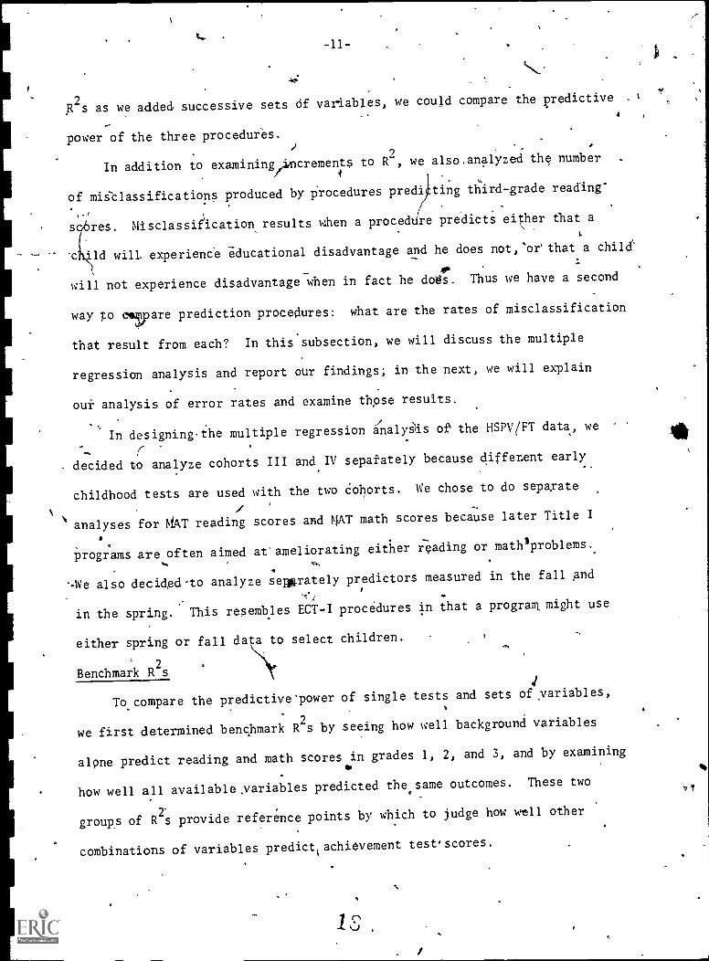
The list of predictor and tutcome variables needs some further explana-

'tion. As one can readily see, we included a wide variety of predictor and

outcome variables in our initial list. Later we found it necessary to

.41

eliminate some predictors and outcomes because too few studies containing

those variables could be located. A few of the variable labels in Table 13

require some description. Items in'the home refer to-family possessions

such as vacuum_ cleaners and television sets, which are often used as indicators

of social class. Other SEgmeasures include scales used to assess

50

a, it

1

1

-40-

Table 13: Predictor and Outcome Variables Sought inStudies Assessed by the Meta-Analysis

Predictor VariablesSex

AgeRaceIncomeFather's EducationMother's EducationFather's OccupationMother's OccupationItems in the HomeOther SES MeasuresSibling VariablesFamily VariablesTeacher Judgement: PK II

' PK I

01

Reading Readiness: PK II

K1

Other ReadineSs: PK IIPK I

K1

IQ Tests; PK II

PK I

K

1

Other oTests: PK II

PK I

K

'1

,Parents' DesiresPrior School Experience

Outcome VariablesReading Achievement 1*

2

3

, 4

5

6

Math chievement 1

2*

3

4

5"

6

Language Arts Ach. 1

2

3

4../

5

6

IQ Test '1

2

34 4

5

6

Composite Achievement 1,

2

3

4

5,

6

Reading Grades 1

2

-, ' 3

4

5

6

Composite Grades 1

2

3

4

5^

:6Other r4asures 1

,2

3

A

6

* Arabic numerals are grade levels: 1 = first grade, 2 = second grade, etc: j

rA

-41-

class.*' Sibling variables refer to such things as number of bro

sisters, birth order, and siblings' eligibility for compensatory education

Family variables inclige measures such as assessment of parent-child inter-

action.

Teacher judgment* and all early childhood tests were grouped according

to when assessment took place. PK II refers to a test time two years prior

to kindergarten; PK I, to oneyear prior. First grade (1) refers to fall

of first plde for teacher judgment and early childhood tests. The other

readiness tests include composite readiness scores and subtest scores other

than reading readiness subtefts.. Other tests include socio-emotional and

psycho-perceptual tests such as the Bender and the Wepman. If we were

unsure where a test fit, we consulted Buros (1972), and followed his

categorization.

Initially, we categorized study outcomes according to achievement,

test scores, IQ test scores, school grades, and other measures, and sought

studies that reported these outcomes measures fo4,the first to the sixth.'

grade. We categorized a first-grade measure as an outcome only if it was

obtained in the spring of first grade. For'other grades, wemade no

'distinction between fall and spring.

Locating Studies

We used several methods to 'find, studies. We made an ERIC search of

)

* Teacher judgment was assessed in a variety of ways, froM 5-point scales

to elaborate questionnaires.

it`

52

A

5

-42-MD'

journals and ERIC documents.* We consulted literature reviews (e.g., Bryant,

Claser, Hansen & Kirsch, 1974) and other meta-analyses (for example, White,

1976); and searched through dissertation abstracts and reviewed the indices

of relevant j urnals for the last ten years.** Finally, we examined the,

bibliographies of articles, books, and reports that we reviewed. In all,

approximately 300'studies were read. These are listed in part II of the

, bibliography.

Criteria for Including Studies in the Analysis

To be included, a,study had to report at least one measure-of a relation-

ship between an early childhood predictor and a later outcome. Most of the

studies we included reported simple correlations. Others reported statisticsS

that could be converted into correlation coefficients. (See Glass, 1977, for

details on converting various statistics to Pearson r's.) Studies that re-

ported only multiple regression analyses without correlatiori matrices were

excldded, since simple r's codld,not be retrieved. Because children develop

rapidly during early childhood, we discarded any study that did not repoft at

least approximate indications of children's ages for the times when predictor

and outcome variables were measured. Some articles reported ages in months,

others in years and fractions of years; and stitil others reported the grades a

seasons when tests were given. To standardizetiur coding of ages, we decide 4record grades and seasons when measurements were Made. Table 14 shows how

we converted ages into grades and seasons. Finally, we omitted'any study

* We first selected all studies with th8 keywOrds'EarlY"Childhood. Then from

all early childhood studies n..4.1e selected those with the keywords Predictive 1.

Validity, Siblings, Achievement, Failure-Success Prediction, Reading Readiness,

'ISES, or Parent-Child Relations.

** The journals were American Educational Nsearch Journal, Child Development,Educational and Psychological Measurement, Harvard Educational Review, Journagof Educational Psychology, Journal of Learning Disabilities, School Review,

and Teachers College Record.

53

-43-

Table 14: Children's Ages and Corresponding Grades and Seasons of the Year

Age (years) m Grade and Season

2.5 to 3.0

3.1 to 3.5

3.6 to 4.0

4.1 to 4.5

4.6 to 5.0

5.1 to 5.5

5.6 to' 6.0

6.1 to 6.6

7 .

8

9

10

11

400

Fall Pre-K II

Spring Pre-K II

IFan Pre-K I

Spring Pr6.4 I

Fall K

Spring K

Fail First Grade (1)

Spr:ng First Grade (1)

SecDnd Grade '(2)

Third Glade (3)

FoLrth Grade (4)

Fifth Grade (5)

Sixth Grade (6)

O

les

--44-

J

47.

that did not report, sample siz e. Based op these criteria of acceptability,

119 of the -300 studie's,initially identified were included in the analysis.

(These are identified witkiasterisRs in part II of the bibliography.) .

Recording Study Characteristics 4

As noted earlier, the magnitude of correlations can vary with study

characteristics. (For example; White [1976] foUnd that a somewhat stronger

relationship between socio-economic class and achievement test scores was

reported in published than in unpublished studies.) Therefore we decided

to record a'wide ranged of such characteristics. Fbr our analysis, we attempted

.to;record'the following information:

Date of theotudy

Author's affiliation

Source of the study(e:g jOurmal)

Number of subjects

Study population(local, regional, etc.)

Percent minority,

in sample

Attrition rate

, Whether children receivedsome special program

Independent. variablet

initial measurementtime

Means of independentvariables

Standartdeviatiort of variables

Reliability of independent variables

Evidence of truncation in independent.variables

Outcome measures'

Outcome measurement time

Meani of outcome measurements

Standard deviations of measurements

Reliability A-outcome measures

Evidence of truncation in outcomemeasures

Correlation between independentvariable and outcome measure

Of course, few studies reported all of these characteristics.

f

55

C -45-

Analyzing the Results

We hAd three main questions in mind when we examined the results of the

meta-analysis:

On average, how does each early childhood variable correlatewith various outcome meaures?

Do some variables have significantly higher cog-relations, indicatingthat they could be better predictors of later outcomes than otherearly childhood variables?

To what extent do the results of the meta-analysis substantiateor differ from our findings from the HSPV/FT study?

Our first step was to calculate the average correlations between predictors

and outcomes.* This resulted in a matrix of 40 predictors by 48 outcome; and

a total of 1291 correlations. Despite the large number of correlations, many

cellS contain few or no correlations. Some predictors, such as PK II tests,

had no correlationS. Some outcomes, including most from the later elementary

grades, had as few as one correlation. We decided to eliminate those pre-

dictors and outcomes that had just a few cases or cases at all: By so

doing we reduced the meta-analysis so that it would more nearly parallel

the data available from the HSPV/FT study. We therefore concentrated on

.

ading, math, and language arts achievement test outcomes at tI4 first,1

second, apd third grade levels, This is much like the HSPV/FT,study, which

has reading and math outcomes in the first three grades. We also pared

down the number of predictors. Still included are the 12 background

variables (sex through family variables in Table 13), teacher judgment,

and the four types of early childhood tests. Again, this set of predictors

* Our unit of analysis in calculating°averages and other statistics wasthe correlation coefficient, not the study; thus some studies contributedone correlation to the analysis, others contributed 20 or 30.

5U

t.

t.

-46-,0

parallels the HSPcr/FT study; but it also permitted us to look at a broader

range of preschool tests than was included in the HSPV/FT data, and at teacher

judgment, which wag.not included in the HSPV/FT data. Appendix A contains

the matrix. of average correlations (821 in all) between all predictors and

the three outcomes reading, math, and language arts achievement test scores.*

/

Appendix B contains correlations (624).between early childhood tests and

the three outcomes.

Some questionsibout the predictive. validity of ECT-I selection variables

Ican be addressed by examining average correlations. Other questions require

further analysiS. When we ask whether some variables do better than others

in predicting later outcomes, we are asking an inferential question, for we-

'

want to know whether differences in correlations are just chance variations.

or are statistically and educationally significant. To answer such questions

'we,prefer,to, use parametric, statistics, which assume normally distributed

variables. Correlation coefficients, however, are not normally distributed.

(See.Fisher, 1915; McNemar, 1969; and Cohen Cohen, 1975). Fortunately,

,

Fisher,devised a method kor transforming correlation into Fisher's

111 .

which approximate normal distributions (Cohen & Cohen, 1975, pp.50t52).

Transforming corrlaens into z's makes it sensible to use analysis,

of variance (ANOVA) and other.pqrametric ptocedures. The next Subsection

illustrates how we used ANOVA to compare the average correlations of dif-.

ferent'earry childhood tests, different outcome measures, and differen

measurement points.

* These correlations are based on a combined sinlole of size of 147,780.

Studies on average had-an n-of 180.

57

-47-

The Findings of the Meta-Analysis

,Discussing the .findings of the meta` - analysis is not easy. We are

examining average correlations from a large number of studies, which vary

in several ways. They .racy in sample size, attrition rates, and other. ,

study characteristics. They vary regarding the predictor variables-(Xis)\ -

employed. They use different outcome measures (Y's). Prediction times (tx)

also vary, as do outcome times (t v). In principle, we could,analyie simul--

taneously all theways in which studies vary. But such an analysis (e.g.,

a four7way ANOVA with several covariates) would bee complex and difficult

to interpret if there were significant interactions. Instead, we have

decidedto examine smaller pieces of the puzzle. We leave to the last a

look at the influence of study characteristics such as sample size, turning

'first to differences resulting from varying predictors, outcome measures,

predictor times, and outcome times. At most we will discuss two-Of these

four dimensions at one tithe. to do this we. will have, to "avenge across"

the other two dimensions. For example, when we-examine the effects of

different outcomemeasures (reading, maih, and language s tests)'and.

different outcome times (first grad', second grade, and third grade), we

average across different predictors (such at types of early Childhood tests)

and predictor-times K, and first grade).

In examining variations in X's, Y's, txIs and t is, we concentrated

on five areas:

Background variables as predictors

Differences in predicting reading, math, and language arts outcomes0

Effect of time between prediction and outcome 411 predictive validity

Predictive validity of different categories of early childhood tests

Predictive validity of teachers' judgment.

5

-48-

We will discuss' eachof these in turn.

Background Variables. Tables 15 and 16 summarize the results for a

set of background variables. We are interested in whether the predictiv,

validity o background variables varies over outcome time (tY) and with

different outcome measures (Y's). Thus we. are looking for effects in these

two dimensions, and we are averaging across the different bac round variables,

(X's). The number in the center of each cell in Table 15 is an average cor-

relation* computed across 12 background variables.** This table and the

accompanying two-way antalYSis of variance 'show two things about the predictive

validity of background variables. First, we see no difference in the overall

ability of background variables to predict different Outcome tests: the mean*

correlations b .Neen background variables and reading tests (.20), math

tests (.17), and language arts rests (.18) are not significantly different

= 1.65, df = 2, 91,p .05). 'second, we find no decrease in the predictive'

power of background variables as they are used to predict later and later

outcomes (first through third grade). The average correlation between back-

ground.variables and first -grade outcomes is actually the lowest, but the

differenCes among means are not significant (F = 2.41, df = 2, 91, p)

These two results parallel what are found in the HSPV/FT data.

Table 16 presents a further comparison between the meta-analysis and the.-

HSPV/FT results. The predictive power of the background variables represented

in, both data sets is similar. Table 16 shows that, witlia few exceptions,

4

* All average correlati-ons arp weighted by the number of cases (i.e., number

of correlations) per cell.

** Sex, age, race, income: father's education, mother's education, father'soccupation, mother's occupation, items in the home, other SES measures, siblingvariables, and family variables.

",..

. ,

Table 15: Average Correlations Between a Set of Background Variables

and Reading, Math, anOranguage Arts Scores,for Three OutcomeTimes*

* , Outcome Time

now

Average:

Outcome Tests Grade 1 Grade 2 Grade 3

Reading

--,-4...27

17 .23

,13..

.22

20

.20

*

Math0.d/

1

.26

5

.16

20

.17

Language Arts11

. 1

- 1-

6

' .11

1

..18

1,,

Column Averages

t,.

'.16.

.23z 19'

*TAIT-lumber in the lower right corner indicates the

number of correlations per cell.

Analysit of., Variance:

Fisher's z by Type of Outcome Test and Time pf Outcome Test

Source ofVariation

Sum ofSquares

oftan.

,Square

Significanceof F.

Main Effects 0.139 41 0.035 1.652 0.169

- Outcome Test 0.070 2 0.035 1.649 0.199.

- Outcome Time 0.102 2 0.051 2.411 0.096

2-Way"Interactions 0.049 4 0.012 0.576 .0.6800.049 4 0.012 0.576, 0.680

Explained ,0:188 8 0.023 1.114 0.362

Residual 1.751 83 0.021

Total 1.939 91 0.021

60

1.

r-50-

.

!.

.-

Table 16: Comparison of Correlations Between Background Variables and..

Outcpmes'from the Me:a-Analysis and HSPV/FT Data Sets (Cohort III). -,* .

BackgroundVariablts

Outcome Tests ar.d Times

Readingf

Reading2 .

-

,Reading

' 3

.

Math1

SexMetaHS/FT

Age

HS/FT

.19

.06 .

.17

.16

.i.

.0);

4_;20

,15, .01 -.02

.

.01

Race

,Meta

HS/FT

.14

. ,36

~/

.23

.21

.16

.23 .

,27

.1.9

.

Inccthe

HS/FT ' .21 :70.17. .14

Mother'sEduc.

MetaHS/FT

, .19

.10'

.34

-.0)

..

---.09 .02

Mother'sOcc.

Meta,HS/FT., -.06

.22

-.07

.10

-.08 -.07

Math Math

_2 - 3

,- ,01

'..00 -.01:

.14

.33

.-

.05

.12

.. 16 ',.

.20

,0

.26

..-.02 -.CP

:

f

-.10 -:.11

4

61 .

-51-

common correlations from the 'two analyses are similar. Like the HSPV/FT data,

the meta-analySis indicates that background variables are modestly correlated,

with achievement outcomes.

Predicting, Different Outcomes._ Table 17 reports average correlations

between early childhood tests and reading, math, and language arts outcomes

at grades 1, 2, and 3. rhe number in the center of each cell is an average

correlation taken across all early childhood tests (reading readiness, other

readiness, IQ, and other tests) at three prediction times (prekindergarten

kindergarten, and grade 1).- All averages are weighted by number of cases

per cell.

Table 17 -and the companion two-way ANOVA show some unexpected results.

Looking at the row averages, we see that the mean correlationsfor rellding

and math putcomes are about the same but that the language arts mean :s

considerably lower, and the analysis of variankn shows a significant difference

among means (F = 8.18, df = 2, 615, p < Instead of theie Hindi gs,

we would expect that early childhood tests would differ in how well theya

predict reading and math scores, since reading and solving math problems

presumably involve quite different skills. We would expect smaller dif-.

ofeiences-in the prediction of reading and language arts scoreL, since the

'underlyip skills are probably more closely related than reading and math

skills.

The analysis of variance also shOws that the-times of,outcome measure-

ments,are significantly different (F = 30.07, df s 2, 615, p <.01). However,

the column means indicate a pattern unlike what we 1,,ould expect. Initially,

'cerrelations.go down -- predictions of first -grade scores do better than

those of second-grade scores. But,third-grade .predictions ate higher than

.w,

.0

-52-

Table 17: Tests as Predictors of Reading, Math, andLanguage' Arts Outcomes*

,

Outcome Times

Outcome TestsGrade 1 Grade 2 Grade 3 Row

Avera

Reading.44

193

.35

121

.38

43

.40

Math.47

27

:4].

12

4 .35

'19

.-

.42

Language Arts.59

.

86

.27

11

88

.34

-35

.33

Column Averages .45. .31 . .36

es

*The number in the lower right,corner is the'number of

Cases pler

6

(2.Analysis of Variance:

Fisher's z By Type of Outcome Test and Time of Outcome Test

Source ofVariation

Sum ofSq ua res

DFMeanSquare

.-44Pm

-Significance

of F

Main Effects 3.550 4 0.888 21.150 0.000

- Outcome Tests 0.686 2 0.343 8.175 0.000

- Outcome Time, .

2.523 2 1.262 30.066 0.000

2-Way Interactions 0.125 4 0.031 0.746 0.561

0.125 4 0.031 0.746 0.561

Explained 3.675 -S 0.459 10.948 0.000, .

Residual 25.808 615 0.042

Total ,, 29.483 623 0.047

93

k

A 11,

41*.

second7grade. This is puzzling, sincewe expect prediction to decline mono-

tonically. This seems to resulefrom some,compiex confounding of study character-.

istics and outcome measurement times. In looking fOr a precise explanation, we

explored the of several characteriSticS. We found, for example, that.

,._

. ..,.

attrition is related to the magnitude of correlationg.' Howbver, we were unable

Att. . . .

.to find a completely s isilaCtoiy-explanation forptse results.

Types of Predictor Tests. Table18 summarizes our4findings for the

!correlations between typeS 0001Ltive tests (reading readiness, other

. readiness,

kindergaTt

math, and

r; and other. tests) given at threw times

n, and first,grade) andthe three outcomeo

language arts). The numbers in the center of each cell are the

(prekindergarten I,

measures (reading,

average correlation across the three outcome Measures (Y's) and the three

ouecome times (y `s) 4

The unadjusted find adjusted means in Table 18 and the analyses of

variance again show some unexpected findings. The unadjusted means and

the ANOVA for type of predicto; test indicateF,that reading readiness tests'

do slightly better than other readiness and IQ tests. Other tests seem to

. do worst. This finding supports our argument in the previous section

that predictive validity should be an important criterion for choosing a

selection test, since not all tests predict equally well. The results

regarding the effects of prediction time on the correlattbn between early

childhood tests and outcomes seems to contradict expectations. The first

analysis of variance (with unadjusted means) shows no significant difference

among the prediction times (F = 1.29, df = 2, 612, p>.0S). Moreover,

the pattern of the unadjusted means is unexpected: tests given` in pre-

kindergarten appear to-,be the best predictors of later outcomes.

At first we thought that there might be 'some confounding bei;veen the ..,

time at which the predictor test-i,.as given and the total time between 4

64

Table 18: Average'Correlations Between Types of Predictor Tests and Later-Grade Outcomes Unadjusted and Adjusted for Time

Predictor Test:

Unadjusted Means -.-. Means Adjusted for Time

Between Measurements

Reading Readiness Tests .47 (264) .47 (264)

'Other Readiness Tests (67) .40 ( 67)

IQ tests .41 ( 80) .40 (,80)

Other Tests -.29 (213) .30 (213)

Predictor Time:

Prekindergarten .42 ( 41) .52 ( 41)

Kindergarten .37 (348) .40 (548)

First Grade :42 (235) .38 (235)

Analysis of Variance:

Fisher'S Z by Predictor Test and Predictor Time

Source of Sum of'Variation 'Squares

DF'Mean

SquareSignificance

of F.

Main Effects 5.522 5 '1.104 28.989 0.000

-Predictor Test 5.010 3 1.670 43.834 0.000

-Predictor Time 0.098 2 "0.049 1.291 0.276

2-11ay Interactions 0.646 J. 6 0.108 2.824 0.010

6-, 0:108 2.824 0.010

Explained 6.167 11 0.561 14.717 0.000-

Residual 23.316 612 0.038

Total 29.483 .623 0.047

Analysis of Variance:

Fisher's : by Predictor Test and Predictor Timeontrdlling Time Between Measurement

Source ofVariation

Sum of

Squares,DF

MeanSquare-

FSignificance

of F

Covaiates 1.069 1% 1.069 29.081 0.000

-1Otal,Time BetweenMeasurement Points 1.069 1 1.069 29.081 0.000

'Main Effects 5.436 5 1.08 29.580 0.000

-Predictor Test 4.430 3 1.4 7 40.176 0..040

-Predictor Time 0.717 2 0.35 9. 52 0.000

0, 2-Way Interactions 0.519 6 0.087 2.354 0.030

0(.519 6 0.087 2.354 0.030

Explained 7.024 12 0.585 15.925 0.000

Residual 22.459 611 0.037

Total 2c).483 623 0.00i3

-55-

predictor test and outcome test. If the time between tests for studies-.

using prekindergarten tests tended to be shorter then the time between

tests when kindergarten and first-grade testsre used, the average cor-

relation from the prekindergarten studies might be equal to or larger than

the averages from kindergarten and,first-grade studies. For example, if

most prekindergarten tests were used to predict first-grade outcomes whereas

most kindergarten and first-grade tests were used to predict third-grade

outcomes, the prekindergarten tests might appear to do as well as or even

better than the kindergarten and first -grade tests. To test this hypothesis,

we entered the total time between tests as a covariate and then performed

thw two-way ANOVA again. The column o usted means in Table 18 shows

that the average correlation for prekindergar en tests increases by

nearly. 25 percent uhile the other means hardly change when time between

tests i taken into account; Moreover, the differences among these -means

become statistically significant (F = 9.75, df = 2, 611, p < 0.001) . This is

a surprising result, quite at odds with our findings from the HSPV/FT data.

A closer examination of the studies that41.

are represented in Table 18

helps explain these results. First, most of the correlations fall in the

kindergarten and-Tirst-grade rows. One might expect that the prediction,

times for studies using kindergarten tests and those usingifirst-grade

tests would differ by about one year on average. But many of the kinder-

garten studies tested in..the spring and all the first-grade studies tested

in the fall because we classified any test given after fall of first grade

as an outcome. Thus, in many cases, the prediction times for kindergarten

and first-grade studies differed by only a few months. This short 'ime

difference may account for finding no difference between the means of

kindergarten and first-grade prediction times.

.66

r

tt

-56-

The high average vaYue for prekindergarten tests may be caused by an

.......,abund*Ola of "good tests in prekindergarten studies. The 41 correlations

of preyndergarten tests with later outcomes come from four studies. Theses$0 .

studies, upon closer examination, use&prekindei=k-a)ten tests that we found

in the HSPV/FT study toNbe g2od predictors of later reading and *h,scores

For example,- one study, reported correlations of 0.60, 0.59, and 0.49

between the WR&T and reading scores at first, 'second, and third grade.4

ese findings are comparable to our results from the HSPV/FT data, which

showed correlations of 0.70 and 0.64 between the WRAT reading subtest and

first- and second-grade reading scores. Thus we would expect the average

correlation for prekindergarten tests to be lower if we had found studies

with a wider range of prekindergarten tests.

The final result of note from Table 18 is the statistically significant\

interaction between test time and test type. We cannot explain this result.

-The interaction,seems to be small in comparison to the main effects, and

4s

we suspect that it is not of substantive significance.

The Predictive Validity of Teacher Judgment

Our final results deal w teacherljudgment as a predictor of later

achievement'. As the Huron field' study (Yui.chak & Bryk, 198a) reported,

teacher judgment is often used explicitly or implicitly to select ECT-I

participlffits.' Indeed, it is often suggested as a complement to or sub-

stitute for test results. We were able to locate studies with a total of

75 correlations between some kind of teacher judgment and reading, math,

and language arts scores in graded 1, 2, and 3.

Table 19 presents a summary of what we, found. Each cell averages

across measures, of teacherjudgment in kindergarten and in first grade.

6"

0

-57-.

Table 19: Teacher Judgment as a Predictor of Reading, Math,

and Language Arts Achievement*

1.

OutCome Time

Outcome Tests Grade 1 Grade 2 Grade 3 Row Averages

Reading.41

27

.56

4

.46

, 6

.43

Math.

0

3311

.,

1

.51

3

. .37

,

Language Arts. 37

..)

/..

.0

.,..)7

1

4

. 37

,

6

Column Averages .38 .56

///'

.47

* The number in the lower riqht corner of each cell is the number

of cases.

fi

.1` .`

4.,

I

ti

4.<e.

-4

r

IPA

-58-

(We found no studies relating teacher judgment during prekindergarten with

Plater outcomes.). Teacher judgment in these studies encompases a range of

activities. In same cases, teachers were asked to rate children's future

achievement on a 5-point scale. In other studies, teachers were asked to

11Pjudge children on the same criteri that the tests used. Still others used

lengthy questionnaires for teachers to aess children. Studios also varied

iOron how long teachers knew the children they asses

nd on whether teachers ,

Y

had seep test results before making their assessment.

Table 10 chows that teachers seem to do well. Average correlations range

from 0.33 to 0.56, which is not much different fromthe correlations for the

best tests in the HSPV/FT data. We did not perfrom an'analysis of variance

on these data, but we can get some useful impressions from the row and column

means. First, there seems to be little differene6 in predicting the three

outcomes, although the average reading correlation is higher than the cor-

relation for math ,or language arts. Second, we do npt see a decline in

.average.correfations as outcome time lengthens. In fact, the. first-grade

average correlation is.lowest of the three. This indicates that teaaOr

judgment may behave like backgtound variables and unlike test sores; i.e.,

the predibtive validity of background variables seems'to be fairly stable,

over time whereas the predietip validity of .early childhood tests declines'

over time.

We need to note an important caveat regarding the studies from which our

, o e "results on teache judgmentwere obtained. Almost all of the correlations

.

%4

. .

(68) measured relationship between teacher judgment In the spring of

kindergarten and test scores in grades 1, 2, and 3. No study reported6

results from the fall of kindergarten, and there were only 7 corrglations"4

.6

7.

-59-

. .

that resulted from f&11 first-grade teacher judgment. Thus one reason teacher

judgment accurately predict later score may be because the teachers knew the

children they were assessing for nearly a full school year. But teacher

judgment used as part of an ECT-I selection procedure would most likely take

place in the fall of the year, when the teachers have known the children they

are assessing for only a short time. Thus we must be cautious about being

overly enthusiastic about teacher judgment until more data are available.

Limitationsand Caveats

Meta-analysis is a new and somewhat controversial analytic technique;

therefore, one must be cautious in its use. As meta-analysis had been used

to synthesize results in more and more areas, critics have raised some im-

.portant concerns (see, for example, Eysenck, 1978; Gallo, 1978; and replies

to Rosenthal and Rubin, 1978). This paper is not the place to examine the

"virtues and vulnerabilities" of meta-analysis in general (see Hauser-Cram,

Note 1, and Jackson, 1980), but it is appropriate t raise some caveats and

0

limitations regarding the results from our application of the technique.

Our use of meta-analysis to examine pdtential ECT-I'selection variabies .

has been an exploratory process. We have sought to move beyond what Glass

and his colleagueS have tried. They attempt a_single meta-analysis -- for

example, synthesizing the. effects of class size on achievement or the effects

of psychotherapy. We, on the other hand, haxie trj,ed to synthesize finding

from several areas simultaneously -- analyzing studies employing one or more

prediction variables from several sets of variables -- background measures,

teacher judgment, and early childhood tests, for example. We have also

attempted to examine a wide range of criterion measures and outComp times.

70

k

-60-

f

Because meta-analysis is a new'approach and because we have applied it

in several ways simultaneously, findings of our analysis must be viewed

cautiously. One way in which we exercised caution was to compare and contrast

the meta-analysis findings with the results from our re-analysis of the

HSPV/FT data. Where results are similar (for .example, those on the pre-

dictive validity of background variables), we are fairly confident of the

meta-analysis findings. But where the meta-analysis produced-results at'

odds with the HSPV/FT data, we are more skeptical. For example, when we

found prekindergarten tests more highly correlated than kindergarten or

first-grade tests with later outcomes, we beganilooking for alternative

explanations. Likewise, although teacher judgment shows promise as a

predictor of later achievement, our conclusions in this regard must be

tentative because teacher judgment was not included in the HSPV/FT data.

Another reason for caution is the complex iejr in which study ter-

istics appear to influence study outcomes. Glass argues that the influence

of such characteristics as sample size can be ignored if the correlation

between the characteristic and the magnitude of the relationship is near

zero; he does not discuss at length what to clef if a relationship is not

near zero. When we looked at the relationships between study characteristics

and magnitude of r's, we found some large and some counterintuitive results.

Table 20 presents correlations between four study charaeristics -- attrition

rate, predictor and outcome reliability, and sample size -- and the size of

r's reported in these studies.

V

Three relationships are statistically significant and two are fairly

substantial. Attrition rate (which is measured by percentage of subjects

A

missing for later measurement) has a strong relationship (0.29) with correlation

71

-61-

r .

Table 20: Correlations Between Magnitude ,of Pearson's r and

Selected Study Characteristics for Studies ReportingRelationships Between Early Childhood Tests and

Reading, Math, and Language Arts Achievement

r

Characteristic Mean Standard Deviation CAes Correlation

Attrition Rate 22.6 20.0 392 .29*

Predictor Reliability 50.3 12.4 404 .31*.

Outcome Reliability 86.0'' 5.0 ' 556 -.03

Number of Subjects 170.0 256.9 624 .10*

*p <.05

72

4-

-62-

size, but it is in the unexpected direction (that is, attrition and the size

of the correlation are directly rather than inversely related). Unless

attrition is random, we would expect correlations to decrease with higher

attrition rates because the sample becoMesjmore homogeneous. Here we find

\the opposite relationship. Predictor reliability is in the expected direction,

but dts relationship with the size of the r's is surprisingly high (0.31)., The

relationship between outcome reliability and cbrrelation size is essentially zero,

probably because of,the low varability in outcome reliability in our sample.

Sample size and magnitude of r's are weakly related with studies'having larger

samples, with large samples tending to produce slightly higher correlations.

It is difficult to know what to make of these relationships. It seems

likely that complex interactions among studies are at work. For example,

it is possible that many, studies of prekindergarteners are done by universities

and research organizations; and, for that reason, perhaps are better can,.

trolled. Predictive validiiy studies of reading readiness tests given to'

kindergarteners and first-graders may be done more often by school districts;

and may be less well controlled. With less well controlled studies, one

would expect reduced correlations between predictors and outcome measures._

To try to unravel these complexities is a substantil task requiring time

1

and resources beyond thos' available to Us. Hence our concern that'the re-

.

sults of our meta Analysis be viewed with caution.

Summary of the Findings from the Meta-Analysis

Overall, our meta - analysis of studies supports the conclusions we reached

from the re-analyzing of the HSPV/FT data 'set.

We found that background variables correlate weakly with '

educational outcomes, but these correlations do not seem to decrease

as the time between prediction and outcome measures increases.

-63-

Some individual early childhood tests predict later outcomes fairly

well; and some tests dd better than others. Reading readiness tests

appear to do best; non-cognitive tests seem to do worst.

o Both analyses revealed significant relationships between predictive

power and time between measurement points, but these relationships

appeared to be more complex in.the meta-analysis data than in the

HSPV/FT data. Probably due to interactions between study

characteristics and the relation of time to predictive power.

oo The meta-analysis data permitted us o examine teacher judgment as

a predictor of later educational ou comes. Our tentative findings

are that teacher judgment does nearly as yell as tests and that its

predictive power seems not to decline over time to the extent test

results do.

CON5LUSIONS

Our aim in this paper has been to inform discussion of ECTJJ selection

policy, and our main. audience' has been people at the federal level who think

about, fc-7,ulate, promulgate, and monitor such policy. Our study has 'een

limited to a discussion of the predictive validity of early childhood-variables

that, in some combination, could make up part of local ECT-I selection strategies.

The study has also been liiited to the data at hand -- data which were collected

originally for other puiposes. In this last section, we will_mention briefly

some considerations besides predictiVe: validity that should be taken into

account in a complete examination of ECT-I selection policy. Then we will

discuss the implications from our findings for ECT-I selection-policy.

Some Other ConsiderationsL

This paper has assessed the predictive Validity of some early childhood

variables that could be part of an ECG' -I selection process. Of course, there

are other criteria for judging selection variableS and for assessing the over-

all process by which young children are chosen to receive ECT-I services. This

subsecti9n will briefly discuss some important considerations that, we have

not discussed in this paper.

i

.74

-64--

Other Aspects of Choosing ECT-I Children. Determining who receives ECT-I

services isliothree-staged process: Title I attendance areas are specified

(on economic grounds), a pool of eligible children residing in the attendance

area is identified (based on educational need), and the neediest children are

.elected from that pool. We have examined only aspects of the, last stage,

selection. But the bther stages need to be considered in any overall dis-

cussion of ECT -1 identification and selection. The second stage, identification,

is particularly problemmatic for ECT-I. Identification for Title I programs.

aimed at children in grades 2-12 is made easier because almost all potentially

eligible children are in school and available for identification. Children 0.

are not so readily available for ECT-I identification since ECT-I programs

often provide the first school experiences for educationally disadvantaged

children. SOMe work has been done om the problem of identifying young children

in need of senices (see Hauser-Cram. Note 2; Yurchak, Note 3), and further

consideration seems warranted.

Costs of Selection Procedures. e have said little in this paper about

the monetary and nonmonetary costs of ECT-I selection, which are obvious

concerns in assessing any selection procedure. We have seen that several

variables together usually predict later outcomes more accurately than one

variable, for example, a test score. But using multiple measures such as a

combination of test scores, background variables, and teacher judgment to

select ECT-I children may be expensive, using resources that might be better

spent serving those children who are selected. Moreover, multiple measures

can be a burden on teachers, children, and parents. Giving several tests,

collecting background information4gand judging children's readiness for

,

school can be anlaborious for teachers d, wors6,1pan take ,time from in

struction. Providing.detailed information about their children can be

f".0, ,

a '-¢5-

annoying or threatening to parents. Data collection, especially test taking,

can be boring, confusing,..br'threatening for children.' Such costs shoilld

be assessed in judging+alternative selectilOn procedures.

Problems in Assessing Yoting Children. In judging variables that could

make:up an ECT-I selection procedure, one must continually keep in mind the

special problems in assessing young children. In another report from Huron's

study of ECT-I evaluations, Haney and Gelberg (1980) not only point out that

"tests and inst ments for use with young children'are geRerallyof loner

technical q

argue tha

ity than those for use with older children" (p. 7) but also

resehoor children of;en lack the physical, intellectual, and

11/

e-czion prereuisits necessary for syste-a: ic assess -ent. given these

1,

special d:ff:tulties it may make sense, esneciall ,hen selectin-g 7rek:nder-

.,

garteners or children who have had no school or preschool experience, to

emphasi:e variables that are,not so dependent on obtaining direct information

from young children in strange 'situations -- variables such as family

characteristics, teacher judgment, and sibling information.- .

a.

Selection Bias. Much of the discussion about'bias against'minority groups

in the literature dwells on the misuse of.standarcliz-ed tests.leading to the

misclaysificationof children. (For example, see Mercer, 1.975). But such

discussions could be broadtned' to other variables 'of a selection strategy:

Haney and KinyaKjui (1979), who airs their discs Sion at tests,provide a

NA

useful perspective on bias. They argue that tests are not usually biased

but the use of tests may be. By extention,7the 'components of an ECT-1

selection procedure (Which might include test score's, background variables,

and teacher judgment, 5oi.example) pr6bably would not be ,intensionally biased -

- -,

for or against minorities.' However, the use of the strategy might be biased.

R

-66-

Haney and Kinyanjui argue'that "a test is biased if, when it is used to make

decisions or inferences about a person or group, those'decisions or inferences

are less valid than those made whqn it is used analagously with people

generally" (p. 5). Their definition of bias rests on thevakidity of the4

decision or inf!yences retulting from the test. Similarly an ECT-I selection

procedure might be said to be biased if the selection decisions for some

groups are less valid than decisions for all children. Furthermore, the

predictive accuracy of a procedure is one criterion in terms of which to

judge its bias. That is, if a variable, a set of variables, or a selection

procedure has lower predictive validity for some group than for others, it

might be viewed as biased.

Implications for ECT-I Selection Policy

mportance of Predictive Validity. The importance of prediction stem's

from the central goal of most ECT-I programs:, ths prevention of educational

problems in later schooling. This goal, together with the requirement of

selecting the neediest children', suggests that selection be based at least

in part on which children are most likely to experience later educational

disadvantage. Thus, we have argued and tried to demOnstrate that the pre-

dictive'validity of background variables, teacher judgment, and test scores

is an important consideration.

The implication here is that local program staff should examine the

predictive validity of their selection method. This means more than just.

looking up a validity index for the tests they use. It means studying the

predictive.validity of their procedures in terms of their unique population

of children, since similar procedures can produce varying results with

different samples,.as we saw in the HSPV/FT re-analysis and the Shipman

OIL

-67-

data, Another reason for encouraging local staffs to examine the predictive

validity of their selection methods is that definitiOns of educational

disadvantage differ.from community to community. Some LEAs are most con-

,'

cerned.about preventing future reading problems; others want to help children4

at-risk become better epared to achieve later school success in general.

Moreover, some LEAs empliasize standardized test scores as measures of . lateri

school success; others are more\interested in grades or students attitudes

toward school. Although we did not find striking differences in how well

early childhood variables predict different outcomes, in some cases, the

composition of a set of variables or the 'Weighting-of the variables that go

into a selection strategy may differ depending upon how a district ch6lekses

to define ed.,:cationaldisadvantage in later grades.

Useful Statistical Procedures. Fortunately, some statistical tools

exist to help local staffs assess the predictive validity of their selection

procedures. We have described two in this paper: examining R2

(and incre-

ments to R2) and examining misclassification rates. Using the latter seems

tto be a particularly fru ful approach to assessing different strategies;1.

it makes explicit the errors and the successes of any strategy and can help

the staff focus their attention on the costs and benefits to the children

they select and do not select.

Importance of Longitudinal Data. Clearly, data collected over time are

needed to assess predictive validity. All the data we used were longitudinal.

The HPSV/FT data set and the Shipman data followed some children from pre-_

kindergarten through third grade. Studies included in the meta-analysis

measured-children as early as two years before kindergarten and as late as

sixth grade. The shortest time span of studies included in themeta-analysis'

was six months -- fall of first grade to spring of first grade.

IP

-68-

Jo judge the predictive validity of a selection strategy, data are needed

at the time of selection and at a future time when some important event will

take place (such as success or failure in third-grade reading). Many districts

have neither the capacity nor the expertise to collect and analyze longitudinal

data. However, given the importance 'of these data'not only for studying

selection but for evaluating programs, help should be provided to LEAsto

enhance their capacity in this respect. Some of this help might come from

Title I 4echnical Assistance Centers. Additional Help migh' come from con-

sortia of LEAs having ECT-I programs. These districts could band together

to share computer facilities, analytic strategies, and even data.

Some LEAs have the capability to collect and analyze longitudinal data

but may lack the resources needed to apply the data to a topic like local

ECT-I selection. One large district we visited had extensive longitudinal

files tracing Follow Through children for several years after the program..

Some files held test scores and background information; other files held

student identification. The only problem was a lack of resources to merge1

these files and apply them to early childhood selection and evaluation

questions. Given the importance of a predictive perspective and the dif-

ficulty in collecting and analyzing longitudinal' data, encouragement and

support fro SED for collecting and analyzing such data seem warranted.

Select nstruments and.Variables. Both the re-analysis of the HSPV/FT

data and the eta-analysis*suggest instruments and variables that have roles

to play in selecting ECT-I children: From the standpoint of prediction, early

childhood tests seem to have a place in selection strategies. Some instruments,

such as the WRAT and the PSI, appear to be fairly accurate redictors of later

7:)

achievement. Others seem to have less accuracy. Thus t e predictive

validity of a test should be considered in -deciding whether to use it.

(

-69-

.,,although some tests have reasonably high predictive validity, we have

seen that adding other variables and assessment methods to test results can

improve the accuracy of a selection p^roever7;e. One set of such variables is

SES-related measures, which usually improve prediction of later achievement.,

and-ido not seem to diminish in predictive power over time spans for which

we had data. In.addition to gl.e background variables such as. income

and parents' educatiop, some ECT-I programs may have access to or the capacity----.

to colleCt more sophisticated variables such as measures of parent-child

interaction. We have little data on the usefulness of such variables for

ECT-I selection, but local-efforts to collect and assess such information

warrant some encouragement and support.

Teacher judgment also has a place in ECT-I selection. Tentative findings

from our meta-analysis show that teacher judgment may do as well as

early childhood tests in predicting later achievement. As we noted earlier,

teacher judgment may be particularly useful in selecting very young children,

whose lack of skills and school experience reduce the reliability and validity

of tests. Unfortunately, we had no data ,plat allowed us to examine how much

. .teacher judgment would add to the predictive power of tests and background

variables. In addition, there seems to be a 'dearth of data on teachers'

ability to assess prekindergarteners.q Clearly, here is an area for futther

research, some of which could be carried on by LEAs with or without TAC

assistance.

Finally, tl e are several potentially fruitful instruments and variables

for which we have no information and for which further investigation is

warranted. We had no data and found no studies that used early-thildhelod

criterion-referenced tests to predict later outcomes, although this use for

80

-70-

CRTs has berry suggested (for example, Stenner, et al., 1976). Parental

judgment islanother area for which we have no data, but where some further

investigation may be warranted (see Johansson, 1965, ;for a s'tudy of pgrental,

judgment in Sweden). In our desdriptive study of ECT-I programs, W'e found

several LEAs using information about siblings and about language proficiency

to select children. Again we cannot comment on these approaches except to

say that they deserve examination.

C

;

-71-

REFERENCE NOES'

Hauser-Cramm,.P. !search synthesis: h.ZITet and vulnerabilitiqs1;/Unpublislied-aper, Kennedy School of Go ertment and Harvard, Graduate

School of ucation 1980.

Hauser-C ,;.P. developmental screening: w and analysis of

"key issue tReport-in preparation for the H o n titute, Cambridge,

MA, 1979.-AP

Yurchak, Mary Ja e.' Identifying and selecting children for early

ng.

childhood Title I° prkrams. Paper in preparation for tha Huron Institute,

-Cambridge, MA, fo hcoMk

4

r

.4

r

82-

S

(4a

vrP

k

. *

-7

,_

,

-72-

REFERENCES

-Z. N...

B eCkeTy W. Teaching reading and language to the disadvantaged. Harvard

tducati nal Review, November 1977, 47, 518-543.,

$ .

Bryant, E.C., Glaser, E., Hansen, M.H., & Kirlch, A. Associations between

, educational outcomes and background variables: A review of selected

literature: Denver, CO: National Assessment -of Educational Progress, q974..

Bpros, O.K. (Ed.. The seventh mental measurements year took. Highland Park,

N.J.: The Gryphon' Press, 1972.

Cohen, J. E Cohen; P. Applied multiple regression/correla analysis forthe behavioral sciences. Hills-dale, N.J.: Lawrence ribaum Associates,

, Publishers, 1975.

Eysenck, H.J. An exercise in mega-silliness. American Psychologist, 1978,

33- 517.

Fisher, R.A. Frequency distribution of the values of the correlation coefficient

in samples from an indefinitely large population. Biometrika, 1915, 10,

507-521.

Gallo, P.S. Meta-analysis--A mixed meta-phor? American Psychologist, 1978,

33, 515-517.

Glass, G.V. Primary, secondary, and meta-analysis of research. Educational

Researcher, 1976, 5, 3-8.

Glass; G:V. Integrating findings:. The meta:analygis of research. In'L.S.

ShulMan (Ed Review of research in education (Vol. 5). Itasca, Ill.:

F.E. Pea6ock P lishers, 1977.

Haney, W.M., The Follow Through planned variation experiment. Vol 5: A

technical history of the nationa4 Follow Through evaluation'. -"Cambridge,

TA: The Huron Institute, 1977. - I

Haney, W.M., &, Gelberg, J.W. Assessment in early childhood education. Cambridge,

MA: The Huron, Institute, 1980.

Haney,' & Kinyanjui, K. Competency testing and equal educgtional oppor-

tunity. IRCD Bulletin, 1979, 14, 1-11.

Jackson, G.B. Methods for integrating reviews. Review of Educational Research,

1980, 50, 438-460.

Johansson, B.A. Criteria of school readiness: Factor structure, .predicttve

value, and environmental influences. Uppsala: Almquist and Wiksells

Boktryckeri.411, 1975. .

4

813

-73- rMcNemar, Q. Psychological statistics (4th ed.). New York: Wiley, 196.

Mercer, J.R. Psych9lpgical assessment and the rights of children. In N.

Hobbs (Ed.) Isstes in the classification of children (Vol. 1). San

Francisco: Jossey-Bass,, Inc 'Publishers, 1975.

0 WY

Molitor, J.A,'., WatkI'ns, M., Qlapidr, D. Education as experimentation:- A

planned variation model, The non - Follow Through study. Cambridge,

.MA:.. Abt Associat 'es, Inc., 1977' .

.

.

.

Nie, NA, Hull, C.H.,,Jenkins, j.G':,45.teinbrenner, K., & Bent, D.H. Statistical

package for the social sciences (2nd EdiA0i.on), New York: McGraw-Hill,

1975. .

Itoverlfhal R., & Rikin, D.C.' 'Interpersonal expectancy effects: The first

143 studies., .Thflehavioral and Brain Sciences, 1978, 3, 377-415. .

.i. ...

_

4 Shipmah, 1;,..C,ficKee.D. ; F BridFeman, B. Stability and change in family.

.

,"`status, situational, and process variables and their relationship to

children's cognitive performance. Disadvantaged- children and their

first. school:experiences:ETS Head Start Longitudinal Study, September,

4,1976. 261'pages. ERIC Reproduction Number ED J38349.

Stenner, N:J., Feifs, H.A., Gabriel, B.R., F DaviS, B.S. Evaluation of the

ESE. A, Title I pr 'gram of the public schools of the District of Columbia,

' '1975-76. Wash gton, D.C.:' The Public Schobls of the District of

Columbia, rio te. 'IP'.

Subkoviak, M.J. Decision-consistency approaches.. In R.A. Berk (Ed.) Criterion-

referenced measures: The state of the are,. The Johns Hopkins University

Press, 1980.

Walker, D.K., Bane, N.J., & Bryk, A.S. The quality of the Head Start planned

variation data (2. Vols.). Cambridge, MA: Th.e Huron Institute, 1973.

Weisberg, H.I,, & Haney, W.M. Longitudinal evaluation of Head Start planned

variation and Follow Through. Cambridge, MA: The Huron Inttitute,'1977.

White, K.R. The relationship between socioeconomic status and academic

achievement. .(Doctoral dissertation, Univ. of Colorado, 1976).

Yurchak, N.J., & Bryk, A.S. ,ESEA Title I early childho4 education: A

descriptive report. Cambridge, MA!' The Huron Institute, 1986.

Yurchak % M.J., Gelberg, & Darman, L. Description of early childhood

Title I programs. Cambridge,-MX: The Hul om institute, 1- 9-79.

e

MOP

4

a.