CT PERFUSION IMAGE PROCESSING: ANALYSIS …amsdottorato.unibo.it/5499/1/Michela_D'Antò_tesi.pdf ·...

Alma Mater Studiorum – Università di Bologna

DOTTORATO DI RICERCA IN

BIOINGEGNERIA

Ciclo XXIV

Settore scientifico-disciplinare di afferenza:

ING-INF/06 BIOINGEGNERIA ELETTRONICA E INFORMATICA

Settore concorsuale di afferenza:

09/G2 BIOINGEGNERIA

CT PERFUSION IMAGE PROCESSING:

ANALYSIS OF LIVER TUMORS

Presentata da: Ing. Michela D’Antò

Coordinatore Dottorato Relatori

Prof. Angelo Cappello Prof. Mario Cesarelli

Prof. Claudio Lamberti

Prof. Paolo Bifulco

Ing. Maria Romano

Prof. Alessandra Bertoldo

Esame finale anno 2013

3

1. INTRODUCTION ................................................................................................................................... 5

1.1 Historical Highlights ....................................................................................................................................... 5

1.2 Specific aims and work task ........................................................................................................................... 6

2. LIVER PERFUSION CT ...................................................................................................................... 10

2.1 Liver physiology ............................................................................................................................................10

2.2 Basis of Perfusion CT .....................................................................................................................................12

2.3 Perfusion CT assessment of hepatocellular carcinoma (HCC) ........................................................................13

3. MATHEMATICAL MODELS FOR LIVER PERFUSION QUANTIFICATION WITH CT ....... 17

3.1 Slope-ratio methods .....................................................................................................................................17

3.1.1 Draining vein assumption method .................................................................................................................. 18

3.1.2 No venous outflow method ............................................................................................................................ 19

3.1.3 Gradient method ............................................................................................................................................. 21

3.2 Measurement of Blood Flow in the Liver with “Slope Method”; Problems and Proposed solutions ..............24

3.2.1 Time of Splenic Peak Method (also called “indirect approach”) ..................................................................... 24

3.2.2 Scaled Spleen Subtraction Method (also called “direct” approach) ............................................................... 26

3.2.3 Slope method: “combined approach” ............................................................................................................. 27

3.3 “Dual input one compartment model” ..........................................................................................................28

3.4 “Deconvolution model” ................................................................................................................................29

4. ANALYSIS OF SOURCES OF VARIABILITY IN PERFUSION CT STUDIES ........................... 36

4.1 Choice of mathematical model......................................................................................................................36

4.2 Imaging Studies used in this Thesis ...............................................................................................................37

4.3 Image processing method to derive perfusion parameters ...........................................................................40

4.3.1 Processing of time attenuation curves ............................................................................................................ 40

4.3.2 Slope method analysis: influence of TAC processing ..................................................................................... 43

4.4 Comparison of maximum slope method and dual-input- one- compartment-model .....................................53

5. SPV INDEX IN CHARACTERIZATION OF ARTERIAL HCC HYPERVASCULARIZATION 56

5.1 Standardized Perfusion Value: Historical background ...................................................................................56

5.2 Sources of Variability in the Use of Standardized Perfusion Value for HCC Studies .......................................57

5.2.1 Material and Methods .................................................................................................................................... 58

5.2.2 Analysis of BFa Variability Due to ROI Manual Selection ................................................................................ 58

5.2.3 Calibration of the CT System ........................................................................................................................... 59

5.2.4 Results ............................................................................................................................................................. 61

4

5.2.5 Discussion ........................................................................................................................................................ 62

5.2.6 Conclusion ....................................................................................................................................................... 65

6. PERFUSION MAPS ............................................................................................................................. 66

6.1 Roi approch vs pixel by pixel approach: the value of perfusion map .............................................................66

6.2 Comparison of maximum slope method and dual-input-one- compartment-model: map based approach ...72

7. CONCLUSION ...................................................................................................................................... 75

REFERENCES .............................................................................................................................................. 77

5

1. INTRODUCTION

1.1 HISTORICAL HIGHLIGHTS

The extraordinary advances in medical technology over recent years have placed imaging at the

centre of cancer diagnosis and assessment but today the information used to direct patient

management is based almost entirely on morphological assessment. However, because of the wide

spread of studies and the increasing interest, functional data will become an integral component of

routine tumour imaging.

It is well recognized that a tumour cannot grow without a blood supply and that assessment of

tumour vasculature provides a measure of tumour aggressiveness as well as insight into other

factors related to prognosis, prediction of response to treatment and risk of recurrence. There are a

lot of functional techniques employed in tumour clinical management but multidetector CT

(MDCT) is widely spread for staging tumours and indeed remains the workhorse of cancer imaging

today. Computed Tomography imaging is a standardized technique used in radiology to visualize

the anatomical structures of the liver and its state of pathology, such as liver tumours. Currently,

perfusion CT has become the most interesting technique for the quantitative study of liver tumour

angiogenesis. The perfusion CT, a technique which require acquisition of image during contrast

agent injection without table movement, allows to quantify important hemodynamic parameters that

play an important role in diagnosis and staging of liver tumours.

This thesis is presented in the environment of liver cancer imaging improvement by the analysis and

application of image processing techniques to liver perfusion CT.

6

Hepatocellular carcinoma (HCC) is the most common malignant liver tumour and is one of the most

common tumours in the world, causing about 1 million deaths per year. It is well known that liver

tumour tissue is characterized by an increased blood supply related to neoangiogenesis. This

process is related with an increase of contrast enhancement on perfusion CT liver images.

Furthermore, primitive liver tumour (HCC) diagnosis, assessment and staging are critical because

PET (Positron emission tomography), that represent the gold standard functional technique, is not a

useful tool in the diagnosis and follow up of HCC, because metabolism of glucose in primitive liver

tumour is not different from the surrounding liver parenchima. So liver perfusion CT studies are

increasingly advocated as a means to assess the grade of vascularization in HCC patients and to

evaluate variations in perfusion parameters following locoregional treatments or antiangiogenic

drugs.

1.2 SPECIFIC AIMS AND WORK TASK

The specific aims at the start of the Ph.D. candidature were to:

• Investigate the basic principles and physics of liver perfusion CT technique

• Investigate the main mathematical modelling used to derive liver perfusion parameters

• Investigate image processing methods to derive perfusion parameters and perfusion maps

• Assess perfusion parameters variability related to different image processing methods

• Assess the value of Standardized Perfusion Value, which represents a new perfusion

parameter, in characterization of arterial HCC vascularisation and generate SPV maps

In clinical application of perfusion CT imaging, there are a lot of technical limits, mainly in image

processing analysis, some intrinsic and others operator-related.

7

So one of the most crucial steps in adopting this technique is the standardization of the

methodology.

Technique’s steps, that are considered in this work, are:

1) Definition of the acquisition protocol and choice of mathematical model to obtain liver

perfusion parameters

2) Time Attenuation Curve fitting

3) Variability related to the operator

4) Variability related to the patient, the acquisition system and calibration of the CT.

5) Analysis of image processing technique, i.e. “ROI based approach” vs “pixel by pixel

approach, i.e. quantitative value of perfusion map

In fact, Perfusion liver CT is spreading as a useful functional technique but no consensus has

emerged about the better image acquisition protocol and the choice of image processing method to

derive tumour liver perfusion parameters. Different mathematical models were applied to obtain

quantitative perfusion parameters from CT perfusion scans but the commonly used model for

describing the contrast enhancement perfusion signal is based on Fick principle, also called “Slope

method”.

Moreover, contrast enhancement and so perfusion values are influenced by patient’s cardiac output

and weight. However, a wide range of perfusion CT techniques have evolved and the various

commercial implementations advocate different acquisition protocols and processing methods. In

this manuscript we analyze different causes of variability related to perfusion CT exams in liver

tumours analysis, testing new algorithms and giving guidelines to reduce the elements of

uncertainty of image processing analysis in the characterization of HCC arterial

hypervascularization.

8

Because some authors indicate that a surrogate functional measurement in Perfusion CT studies (as

Standardized uptake value in PET studies) would be useful in characterization of tumour

neoangiogenesis, we have developed an algorithm to calculate from region of interest and pixel-by-

pixel analysis a SPV index. The significance of SPV index in characterization of arterial HCC

vascularisation was also assessed. Such software would be directly analogous to SUV software

currently implemented on PET system. In conclusion, although Perfusion CT present some

limitations in the processing analysis, this techniques are becoming an important tool in medical

research and in clinical practice.

The research activities, described in this thesis, have produced scientific results published on

scientific journal or presented at national and international congresses. Below the list of all the

publications is reported:

- Papers published on scientific journal:

• M. D’Antò , M. Cesarelli, F. Fiore, M. Romano, P. Bifulco, A. Vecchione. Sources of

variability in the use of standardized perfusion value for HCC studies. Open Journal of Medical

Imaging. 2012, 2, 33-40

- Abstract of papers presented at National and International congresses:

• M. D’Antò , M. Cesarelli , P. Bifulco , M. Romano , F.Fiore , V.Cerciello , T.Cerciello

“Perfusion CT of the liver: slope method analysis”. Secondo Congresso nazionale di Bioingegneria,

Torino 2010, Atti Pàtron editore. pp. 467-468

• Michela D’Antò , Mario Cesarelli, Paolo Bifulco, Maria Romano, Vincenzo Cerciello,

Francesco, Fiore, Aldo Vecchione. “Study of different Time Attenuation Curve processing in Liver

CT Perfusion”. 10th IEEE International Conference on Information Technology and Applications in

Biomedicine Corfù, Greece, 2010, paper N. 101

9

• Presidente, M. Romano, R. D'Angelo, F. M. Ronza, M. Cesarelli, F. Fiore, M. D'Antò . “A

new procedure to obtain Standardized Perfusion Value to assess HCC vascularization: early

clinical experience” European Congress of Radiology, Vienna, 2011

• M. D’Antò , M. Cesarelli, P. Bifulco, M. Romano, R. D’Angelo, F.Fiore “Parametric

mapping of the Standardized Perfusion Value in Hepatocellular Carcinoma”, European Congress of

Radiology, Vienna, 2012

• F. Fiore, M. D’Antò , S.V.Setola, P. Bifulco, M. Romano, M. Cesarelli, “Cause di

variabilità nell’applicazione dell’indice di perfusione Standardized Perfusion Value nei pazienti con

HCC” 45 Congresso SIRM 2012, Torino

• M. D’Antò , F. Fiore, M. Romano, P. Bifulco, M. Cesarelli “Reliability of perfusion maps in

HCC patients” GNB2012, June 26th-29th 2012, Rome, Italy

10

2. LIVER PERFUSION CT

This chapter presents the theory of Liver Perfusion CT technique. The physiological process of liver

tumour vascularisation is described.

2.1 LIVER PHYSIOLOGY

The liver has a unique perfusion system with a dual blood supply. More than two-thirds of the

blood supply comes from the low-pressure portal vein, and the rest comes from the high-pressure

hepatic artery. The capillaries of the liver, called ‘sinusoid capillaries’, therefore contain a mixture

of portal and arterial blood. The sinusoid capillary system is very dense, representing almost one

third of the volume of the liver parenchyma. The endothelial cells that line the sinusoids are

anatomically and biologically different from endothelial cells in other organs.

Figure 1: The liver is supplied more than two-thirds by the portal vein and less than a third by the hepatic artery. A

transverse slice through the abdomen allows simultaneous measurement of the attenuation in regions of interst (ROIs) drawn

in the portal vein, in the aorta, and in the liver tissue.

They lack a basement membrane and contain fenestrae, characteristics that facilitate the transport of

nutrients and macromolecules between the sinusoids and the hepatic parenchyma. The hepatocytes

11

lining the sinusoids represent most of the volume of the liver parenchyma, and the interstitial space,

called the ‘space of Disse’, is almost virtual, representing only 10% of the total liver volume.

Specialized pericytes called stellate cells (or Ito cells) are located in the space of Disse and wrap

around the walls of the hepatic sinusoids. Regulation of blood flow and vascular resistance in the

hepatic microvasculature are intimately linked. Whereas in most organs the site of blood flow

regulation occurs at arteriolar level, in the liver most of the blood flow enters at low pressure

through the portal vein, and resistance changes occur in the sinusoid. Stellate cells play a role in the

regulation and control of blood flow through the liver based on their anatomic location and

contractile characteristics by modulating the sinusoidal caliber in response to several vasoactive

endothelium derived mediators including nitric oxide (NO). The portal supply varies greatly during

the day in relation to bowel activity, with large increases in the postprandial periods. The total

hepatic blood supply, however, is finely tuned by the so-called ‘hepatic arterial buffer response’,

which is the inverse response of the hepatic artery to changes in portal vein flow. These intrinsic

regulatory mechanisms based on the local concentration of adenosine tend to maintain total hepatic

blood flow at a constant level, allowing an increase in the arterial blood supply to compensate for a

decrease in portal supply, and a decrease in arterial blood supply in cases of increased portal supply.

It is important to note that, in contrast, variations in arterial blood supply cannot be compensated by

variations in portal supply.

The specific dual perfusion of the liver makes it more difficult to analyze it with contrast-enhanced

imaging than the perfusion of other tissues. The enhancement curve of the liver, after the injection

of a bolus of contrast agent, is the combination of the enhancement due to the contrast agent

flowing in the arterial blood and the contrast agent flowing in the portal blood. Whereas the

molecules of contrast agent arrive quickly when they are delivered to the liver through the arterial

route, they are delayed and diluted by the splanchnic circulation when they are delivered through

the portal route.

12

Many strategies have been developed to take advantage by the portal lag to separate and quantify

the arterial and portal hepatic perfusions. A comprehensive review of perfusion imaging of the liver

has recently been published by Pandharipande et al [1].

2.2 BASIS OF PERFUSION CT

Perfusion CT technique typically requires a baseline image acquisition without contrast

enhancement followed by a series of images acquired over time after an intravenous bolus of

conventional contrast material. Because blood attenuates X-rays uniformly on the scale of the

spatial resolution of a CT scanner, flowing blood cannot be differentiated from stationary blood. To

measure tumour perfusion with CT, a contrast agent is injected intravenously, to ‘label’ the blood.

Assuming that the injected contrast is uniformly mixed with blood, tracing blood through the

tumour circulation is equivalent to tracking a bolus of contrast through the tumour. As such, we can

make use of the extensive literature on tracer kinetics modelling in the measurement of CT tumour

perfusion. Note that in this thesis we use the terms perfusion and blood flow interchangeably. Blood

flow (F) can be defined as the volume flow rate of blood through the vasculature in a tumour. It is

usually expressed in units of ml/min/100g or ml/min/100ml.

Also, in the diagnosis of tumour or the study of tumour biology, it is highly advantageous that

besides perfusion we can measure additional functional parameters in the same study.

The fundamental processes underlying CT measurement of tumour perfusion and associated

hemodynamic (functional) parameters are the transport by blood flow of an intravenously

administered iodinated contrast agent to the tumour. With the current fast CT scanners tissue

contrast concentration can be measured and traced over time at short intervals to allow detailed

modelling of the distribution of contrast agent in tissue. In fact the resulting temporal changes in

contrast enhancement, often displayed as time attenuation curves (TAC) (Fig. 2) are subsequently

analyzed to quantify a range of parameters that reflect the functional status of the vascular system.

13

Compartmental models and linear systems based methods for contrast transport and exchange have

been developed to quantify tumour blood flow, blood volume, mean transit time, and other

parameters (see the following chapter for details).

Figure 2: An example of Time attenuation curve (TAC). This curve has been obtained positioning a ROI (Region of interest)

on aorta. Blue points represent means of HU values inside the ROI and were computed for each slice of the sequence (at

different acquisition time) to compute a mean tumour-TAC.

2.3 PERFUSION CT ASSESSMENT OF HEPATOCELLULAR CARCINOMA (HCC)

Folkman and colleagues [2], in the 1960s, first proposed the dependence of sustained tumour

growth on angiogenesis, a relationship that continues to be heavily explored today [3][4]. In patients

with cirrhosis, a spectrum of nodules, including benign regenerative nodules, dysplastic nodules,

and HCC, can form; differences in their respective blood supplies can assist in their detection and

characterization [5][6][7][8]. Regenerative nodules, like normal liver parenchyma, continue to

receive a majority of their blood supply from the portal vein, whereas the evolution from a low-

grade dysplastic nodule to frank HCC is associated with a progression toward increasing arterial

blood supply [5][6][7][8] (Fig 3).

14

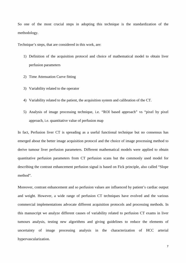
Figure 3: Diagram shows physiologic basis of perfusion imaging for tumor surveillance. Progressive increase in arterial

versus portal venous supply is associated with both the evolution from a low-grade dysplastic nodule to frank HCC and the

development of a metastasis from a circulating tumor cell.

During this evolution, sinusoidal endothelial cells are recruited to create an arteriolar network that

gradually replaces normal sinusoidal architecture, and this process is known as “capillarization” [5].

At histological analysis, dysplastic nodules and HCC manifest neoarteriogenesis, which takes the

appearance of unpaired or nontriadal arteries, that is, arteries not associated with portal vein

branches [5][7][8]. Vascular endothelial growth factor expression, a marker of angiogenic activity,

has been found to increase linearly and parallels the development of unpaired arteries [9]; it is

negligible in regenerative nodules, moderate in dysplastic nodules, and strong in HCC [9]. Given

this progression, serum vascular endothelial growth factor levels in patients with HCC have been

explored as markers of tumor activity [10] and as predictors of postoperative tumour recurrence and

survival [11].

15

Figure 4: Neoangiogenesis process in tumour development

Perfusion CT studies are increasingly used in the HCC imaging. This aspect is facilitated by the

current availability, on the market, of multislice spiral CT systems and commercial software

packages and promoted by the diffusion, in routine clinical practice, of anti-angiogenic therapies.

Neoplastic angiogenesis is in fact an important prognostic factor and a promising target for new

treatments, of fundamental importance for monitoring tumour growth. Different techniques of

image processing have been employed, in recent years, to obtain information about angiogenic

characteristics of tumours in a non-invasive way. Among them, CT perfusion is advocated as a

means to assess the grade of vascularisation in tumour tissue. This is supported by studies, which

have reported a correlation between contrast enhancement parameters and histological

measurements of angiogenesis [12,13]. CT perfusion is also employed to evaluate variations in

perfusion parameters following regional treatments in loco or antiangiogenic drugs [14][15][16].

The clinical value of perfusion CT in the assessment of HCC and its correlated hypervascularization

is confirmed by a lot of literature in this field. In the last two decade numerous studies have

confirmed that perfusion CT is one of the best imaging acquisition technique to characterize HCC

lesion [17][18][19].

16

Arterial hypervascularization is considered an essential aspect to evaluate the grade of

aggressiveness of HCC tumour. In fact tumor HCC angiogenesis induce an increase of

vascularisation in tumour which is reflected by an arterial blood flow increment in CT perfusion

exams. In normal liver parenchyma arterial hepatic component is about 20 ml/min/100ml. Values

greater than 40-50 ml/min/100ml are compatible with HCC lesion [20][21][22][23][24].

17

3. MATHEMATICAL MODELS FOR LIVER PERFUSION QUANTIFICATION

WITH CT

Since perfusion CT has been introduced in clinical practice different mathematical model have been

applied to TAC to obtain quantitative perfusion parameters. In this chapter the principles of these

mathematical modelling for liver perfusion quantification are described.

3.1 SLOPE-RATIO METHODS

The basic model is very general and since the derivation of similar techniques by Fick in the 1870’s,

has been applied to tracers as diverse as dye and heat as well as CT contrast. Slope method is based

on a compartmental analysis, often termed a black box analysis. The contrast material is modelled

as entering an organ via an artery and rapidly distributing itself uniformly within the blood vessels

and extra cellular space, and then, after a short interval, starting to leave the organ via a vein, see

Figure 5.

Figure 5: Black box model of flow and typical time attenuation curves (TAC) , where a(t) is the concentration of contrast

material in arterial blood showing a recirculation peak, c(t) the concentration of contrast material in the tissue and v(t) the

contrast material concentration in the draining vein.

18

A simple approach of this sort can be used to model and calculate perfusion.

3.1.1 DRAINING VEIN ASSUMPTION METHOD

At any time t, let a(t) be the arterial concentration of contrast agent, v(t) be the venous concentration

and c(t) be the tissue concentration within a volume of tissue to be examined. Consider a volume of

tissue, V, corresponding to a voxel and the flow into this volume as F. Then by definition, the

perfusion P of the voxel is F/V. Consider the time interval (t, t+δt). The amount of tracer arriving in

the voxel is Fδ t[a(t) – v(t)]. This is the change in the amount of tracer in the voxel, i.e. the change

in [V c(t)].

Thus

1. δ�c�t�V� Vδ�c�t� � Fδt��

Going to the limit and integrating with respect to t:

2. P ��

� ��

��

Figure 6: Draining vein assumption Perfusion can be expressed as tissue concentration at time t, c(t), divided by difference

between the area under arterial curve, ∫a(t), and the area under the venous curve, ∫c(t).

Thus if artery, venous and tissue concentrations are able to be determined, perfusion can be

calculated, see Figure 6. This approach has been used with radioactive tracers using probes

positioned over the organ and arterial and venous blood sampling. Unfortunately few imaging

systems, including standard CT or MRI, can simultaneously measure input, output and parenchymal

areas easily.

19

To determine perfusion we wish to sample the change of tracer concentration over a comparatively

short period of time, so we require more rapid imaging. Rapid imaging is generally limited to a

single section of the patient in which it is difficult to obtain an image of the organ, its artery and

vein. Fast electronbeam CT scanners are an exception, as they can very quickly acquire a series of

transaxial slices. They have been used to study perfusion, notably cardiac perfusion, using the

formulation described above.

3.1.2 NO VENOUS OUTFLOW METHOD

A more realistic situation is imaging of arterial and tissue concentrations but not venous

concentrations. If a bolus of tracer is given in a reasonably short time, we may assume that the

venous outflow of tracer is negligible for a time less than the transit time of the tracer through the

organ. Let this time be tven . Thus v(t) = 0 for t< tven, so that from equation 2:

3. � �� !

� (t<tven)

To minimize error this ratio is determined when the numerator and denominator are at their

maximum. Let tmax be the time of peak parenchymal contrast concentration and as long as;

tmax < tven

4. � ��"#$� �� !"#$

�

If the time for the tracer to complete a loop of the entire vasculature system is less than the time to

maximum concentration in tissue, the arterial concentration curve shows peaks due to re-circulation

of the contrast material. The first pass phase of a contrast material is often modelled by a gamma

variate fit to avoid the peaks due to re-circulation.

The arterial concentration is modelled using the gamma fit as

20

5. �� %� � & �' ()�!)!��

*

Where a(t) is the modelled increase in vascular contrast over baseline, t is the time, t0 is the arrival

time of the contrast at the vascular region of interest, see Figure 7.

Figure 7: Arterial gamma variate fit to correct for recirculation. The arterial concentration curve, a(t), is modelled by a

gamma variate fit, a*(t), to limit the effect of the recirculation of the tracer on the area under the arterial curve.

When a gamma variate fit is applied to the arterial time concentration curve a model of first pass

curve is produced a*(t). This modelled curve does not have the recirculation peaks. Thus the area

under this curve approximates the total contrast delivered to the organ without errors due to

recirculation.

Thus we can calculate:

6. � �+ � �, -&

which is a measure of the area under the arterial curve if we had a tracer that did not undergo re-

circulation. The reason for doing this is to allow the denominator of Equation 4 to be independent of

tven, the time of venous outflow appearance. There remains the assumption that the c(t)max occurs

prior of the recirculation and it is thus unaffected by recirculation of contrast material.

Perfusion is then calculated as

21

7. � ��"#$� �+.

� ��

Figure 8: Arterial gamma variate area and maximal tissue enhancement.

Thus: Perfusion is the ratio of the maximal tissue enhancement to the area under the arterial time

attenuation curve.

In literature, this relationship is variously referred to as the Sapirstein Principle, the Single

Compartment Formulation or the Mullani-Gould formulation see Figure 8. This often

underestimates higher values of perfusion with intravenous injection because the assumption of “no

venous washout” is violated. Thus to apply this method we require that the time to peak of the

tissue time-density curve (which is related to the width of the input bolus) is shorter than the

minimum transit time of the system. The method can be applied to the abdomen using a time

enhancement curve from an aortic region as an ‘input function.’ Note that this implies that we

assume that there is no significant broadening or perturbation of the time enhancement curve

between the aorta and the afferent arterioles. This is generally the case but the assumption would

fail in the case of a stenosis between the aorta and the relevant afferent arterioles.

3.1.3 GRADIENT METHOD

A variation of this formulation for perfusion can be obtained if we differentiate equations 2 to 4,

obtaining:

22

8. � /0�!�

/!��1��

from equation 2 and

9. � /0�!�

/!�� ( t < tven)

from equation 3. Again minimizing the error by using the peak value of the denominator and

numerator we use t*max the time of the peak ‘gradient’ of parenchymal enhancement where t*

max <

tven. we obtain:

10. � /0�!�

/! "#$��"#$

11. �(2345678 9:�; <=� >:?� @A �B: C>DDE: C>F: G?B�?�:F:?� 9:�; H=�:=>�I G?B�?�:F:?�

This assumes there is minimal distortion of the vascular time enhancement curve in the passage

from the imaged artery and the afferent arteriole, i.e. maxima are identical. Thus it is no longer

necessary to perform a gamma fit of the arterial curve to obtain the area under the curve unaffected

by re-circulation as only the peak value is required, see Figure 8.

Figure 9: Peak arterial enhamcement and peak gradient of tissue time enhancement curve

However, a gamma fit could still be applied to the arterial time enhancement data to reduce the

underestimation of the peak enhancement due to the peak falling between two discrete sampling

23

points. This gradient approach was proposed by Peters et al.[25][26] for use in nuclear medicine

studies and adopted for dynamic contrast-enhanced CT by Miles et al.[27][28][29]. The gradient

method has the advantage that the tissue time-enhancement curve reaches its peak gradient well

before its peak value. Thus the assumption that there is no venous outflow prior to time of the peak

gradient rather than the longer time to peak is less likely to be violated. The use of early datum

points to obtain a perfusion value also means that in imaging based modalities there is less likely to

be patient movement due to breathing and may enable single breath hold imaging if the time to

maximum slope for the organ of interest is sufficiently short. However this technique is innately

more affected by noise as we are differentiating the data set. The gradient method, while having a

shorter time required to determine the perfusion, may still have a time to maximum slope that is

longer than the transit time in organs with a short transit time. This will lead to the breaking of the

assumption of no venous outflow. The slope of the tissue enhancement curve and the time taken to

reach the maximum slope are dependent on the bolus volume, the rate of injection and the patient’s

cardiac output.

The figure 10 presents a graphical representation of the three methods for perfusion determination

based on compartmental analysis.

24

Figure 10: Schematic representation of compartmental model based perfusion calculation methods

3.2 MEASUREMENT OF BLOOD FLOW IN THE LIVER WITH “SLOPE METHOD”; PROBLEMS

AND PROPOSED SOLUTIONS

There are several published studies that have considered perfusion in the liver. To date these have

principally used the gradient method. The objective has been to attempt to quantify both arterial and

portal perfusion. This requires to separate the effect of contrast arriving with the arterial blood from

the portal blood arriving a short time later, and determining the magnitude of the two inputs.

3.2.1 TIME OF SPLENIC PEAK METHOD (ALSO CALLED “INDIRECT APPROACH”)

Miles et al. [28] described liver perfusion imaging using CT in 1993 by generating enhancement

curves from regions of interest (ROIs) drawn over the liver, the aorta, and the spleen after a bolus

injection of contrast agent.

25

Liver enhancement was resolved into arterial and portal venous components by assuming that

maximum splenic enhancement marks the end of the early arterial phase and the beginning of the

delayed portal venous phase of liver perfusion.

They assumed that prior to the time of the splenic peak there would have been no contrast from the

spleen or other organs feeding the portal vein, thus up until this time, the liver could be considered

to be supplied with only arterial contrast. This allows the arterial perfusion to be determined in the

usual way:

Perfusion = Maximum liver gradient / Maximum arterial enhancement

The portal perfusion was calculated from the maximum slope of the remainder of the liver curve

over the arterial enhancement, see Figure 11.

Figure 11: Arterial and portal perfusion phases of liver enhancement. a(t) Arterial enhancement. l(t) Liver enhancement

curve showing maximal slopes contributing to arterial and portal perfusion. These phases are separated by the time of splenic

peak enhancement.

This approach will lead to an underestimate of the portal perfusion for two reasons. The maximum

enhancement of the portal blood supply will not be the same as that of the arterial. It will be lower

due to dilution and broadening of the bolus in its transit through the spleen and other visceral

organs. In addition the increase in enhancement due to the arrival of contrast in the portal blood will

be masked by the reduction of contrast as the arterial blood flows out of the organ. The outflow of

arterial contrast leads to an under estimate of the maximum slope due to portal contrast.

Nonetheless this approach has shown clinical utility. However the method requires that the spleen

be imaged in the transaxial slice.

26

The maximal slopes of the liver time–density curve in each phase were divided by the peak aortic

enhancement to calculate both arterial and portal perfusion (BFa, BFp). The hepatic perfusion index

(HPI), which is the ratio of the arterial perfusion to the total hepatic perfusion (HPI = arterial

perfusion/ arterial + portal perfusion) was also calculated. HPI is also known as the ‘Hepatic

Arterial Fraction’.

This technique is simple to implement and can be applied to any segment of the liver, as there is no

need to include the portal vein or major portal vessel within the tissue imaged. However, the

method underestimates portal hepatic flow for two reasons: first, the downwards slope of the last

part of the arterial time–attenuation curve is superimposed on the upwards slope of the arriving

portal curve; and second, the maximal slope of the portal venous phase of enhancement is divided

by the peak aortic enhancement instead of the peak portal enhancement, which is flattened and

diluted after flowing through the splanchnic system.

3.2.2 SCALED SPLEEN SUBTRACTION METHOD (ALSO CALLED “DIRECT” APPROACH)

To avoid these limitations, Blomley et al.[30] modified this approach by subtracting the arterial

phase liver enhancement (modelled after splenic enhancement) from the liver enhancement curve to

give a more ‘accurate’ portal time–attenuation curve. From this corrected curve, portal perfusion

was calculated by dividing the slope of the rise in attenuation during the portal enhancement phase

by peak portal venous enhancement itself.

Figure 12: Liver enhancement curve as the sum of Arterial and Portal phases.

27

This ‘corrected approach’, however, has two main limitations.

Figure 13: Portal enhancement as the difference of liver and scaled spleen.

First, it assumes that hepatic arterial and splenic enhancement curves are similar. Such similarity is

unlikely in view of the unique microcirculation within the spleen, recognized as the mechanism

underlying the transient splenic inhomogeneity seen during contrast-enhanced CT.

Second, the technique requires a set of slices containing both the portal vein and a part of the spleen

to be able to draw ROIs and extract the enhancement curves.

3.2.3 SLOPE METHOD: “COMBINED APPROACH”

This method was introduced by White et al in 2007 and applied to liver perfusion MRI imaging. By

literature analysis, it is possible to state that two main methods have been proposed for deriving

perfusion measurements and HPI from CT time–density information. Both calculate arterial

perfusion part by dividing the peak gradient in the liver during arterial phase by the peak

enhancement of the aorta, but they differ in their approach to estimating portal perfusion. In the

‘‘indirect’’ approach portal component is calculated as the peak gradient in the liver during portal

phase divided by the peak arterial enhancement.

12. JKL /0�!�

/! MNO!��"#$

28

Two refinements are made in the ‘‘direct’’ approach: the arterial component of hepatic uptake is

removed before measuring portal uptake gradient (by subtracting a scaled enhancement curve from

a purely arterial organ such as the spleen), and perfusion is estimated by dividing this corrected

portal by peak enhancement measured in the portal vein.

Both techniques have been reported to show differences in perfusion between control subjects and

patients with malignancy [30][28][31] but the ‘‘direct’’ method is more physiologically appropriate

and, when applied to dynamic CT, provides portal perfusion values in closer agreement to those

derived using other techniques [31]. This method is also less subject to errors arising from arterial

washout and recirculation.

In ‘‘combined’’ method, portal perfusion is derived from gradient after subtraction of the arterial

component from the liver curve (as in the direct method), but scaled to the enhancement of the aorta

rather than that of the portal vein.

This approach makes the implicit assumption that a single blood concentration of contrast agent is

applicable to both the arterial and portal perfusion, as in the ‘‘indirect’’ method used for dynamic

CT measurements of the HPI [28]. However, since the relative hepatic and portal perfusion are both

scaled to the peak of the aortic enhancement curve, this scaling factor appears in both the numerator

and the denominator of the HPI and can be omitted entirely when only the HPI values are required.

The ‘‘combined’’ method therefore lends itself to voxel-based HPI analyses because it removes the

need for measurement of the aortic and portal venous concentrations of contrast agent. This enables

the HPI analysis to be performed with minimal operator intervention, using rapid lower-resolution

dynamic scans where the portal vein is difficult to isolate and where saturation effects in the aorta

are hard to eliminate.

3.3 “DUAL INPUT ONE COMPARTMENT MODEL”

Van Beers and Materne have developed a compartmental model with a dual-input [32][33]

29

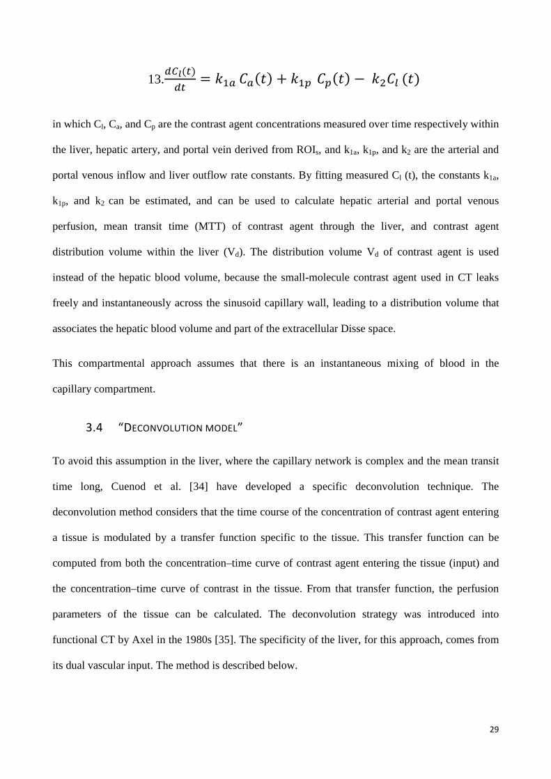
13. PQ��

� %R� S�� T %RU SU� � � %VSI � �

in which Cl, Ca, and Cp are the contrast agent concentrations measured over time respectively within

the liver, hepatic artery, and portal vein derived from ROIs, and k1a, k1p, and k2 are the arterial and

portal venous inflow and liver outflow rate constants. By fitting measured Cl (t), the constants k1a,

k1p, and k2 can be estimated, and can be used to calculate hepatic arterial and portal venous

perfusion, mean transit time (MTT) of contrast agent through the liver, and contrast agent

distribution volume within the liver (Vd). The distribution volume Vd of contrast agent is used

instead of the hepatic blood volume, because the small-molecule contrast agent used in CT leaks

freely and instantaneously across the sinusoid capillary wall, leading to a distribution volume that

associates the hepatic blood volume and part of the extracellular Disse space.

This compartmental approach assumes that there is an instantaneous mixing of blood in the

capillary compartment.

3.4 “DECONVOLUTION MODEL”

To avoid this assumption in the liver, where the capillary network is complex and the mean transit

time long, Cuenod et al. [34] have developed a specific deconvolution technique. The

deconvolution method considers that the time course of the concentration of contrast agent entering

a tissue is modulated by a transfer function specific to the tissue. This transfer function can be

computed from both the concentration–time curve of contrast agent entering the tissue (input) and

the concentration–time curve of contrast in the tissue. From that transfer function, the perfusion

parameters of the tissue can be calculated. The deconvolution strategy was introduced into

functional CT by Axel in the 1980s [35]. The specificity of the liver, for this approach, comes from

its dual vascular input. The method is described below.

30

Deconvolution allows the determination of the theoretical impulse response of the tissue, that is, the

time course of concentration that an instantaneous input of contrast material (impulse input) would

have yielded.

When the contrast agent enters the tissue as a function of time, Ci(t), the time course of the

concentration of contrast throughout the tissue depends both on the time course of a theoretical

impulse input (instantaneous input) through the tissue, h(t), and on the actual experimental time

course of contrast input.The concentration–time curve at the venous outflow, Co(t), is the

convolution of Ci(t) by h(t):

14. S@� � S>� � + W� �

However, since we cannot measure the time attenuation curve at the venous outflow of the tissue

and can only measure the concentration–time curve of contrast into the tissue, we have to infer the

venous outflow time attenuation curve from the tissue time attenuation curve. To do so, we use the

notion of residue function. The integral of h(t) is:

15. X� � � W�Y�,Y�&

31

Figure 14: Relations between the residue function R(t), the cumulative frequency function H(t), and the probability density function h(t). The contrast agent that progressively leaves the tissue accumulates outside the tissue. At the venous outlet the

concentration of contrast agent rises progressively before decreasing to zero. The initial value of R(0) is normalized to one, as well, therefore, as the final value of H(t) and the area under the curve h(t)

where H(t) is the fraction of an impulsive input which has already left the tissue by time t (Figure

14). It is called the cumulative frequency function. Its complementary function is called the residue

function R(t):

16. Z� � 1 � X� �

where R(t) is the fraction of the impulsive input remaining within its distribution volume Vd in the

tissue at time t. The concentration–time curve of a tracer remaining in its volume of distribution

within the tissue Cd(t) can be predicted for any type of input function, Ci(t), as the convolution of

Ci(t) by R(t):

17. S � � S>� � + Z� �

Because the distribution volume Vd of the tracer is within a larger volume of tissue Vt, the

concentration of tracer within the tissue is:

32

18. S�� S � �\ �

where Vdt = Vd/Vt is the fractional dilution volume of the molecule expressed as a percentage of the

total volume of tissue Vt. The concentration of tracer in a voxel of tissue Ct(t) is therefore the

convolution of Ci(t) by Rt(t), the tissue transfer function (Rt(t) = [VdtR(t)]):

19. S�� S>� � + Z��

After contrast injection, a deconvolution process can allow the determination of Rt(t), knowing the

contrast variation of the tissue Ct(t) and the input function Ci(t). For finite time sampling steps of ∆t

= T, the convolution Ct(t) = Ci(t)*R t(t) can be approximated by the following sum:

20. S]�8^� + Z��8^� ^ ∑ S>�8^ � %^�Z��%^�;`?�R;`&

The category of Weibull functions

21. a� � � (bL)!c0

has been chosen to represent the tissue transfer function Rt(t) because its shape is intermediate

between a falling exponential function and a square function, resembling the supposed liver curve.

A computer program is necessary to minimize the quadratic error between the measured tissue

response Ct(nT) at each time nT and the assumed response Ct*(nT) after convolution of the

measured input Ci(nT) at each time nT:

22. S�+�8^� ^ ∑ S>�8^ � %^� � (bL�dec

0;`?�R;`&

The program yields the value of the three unknown factors a, b, and c, allowing the estimation of

Rt(t) (equation 19). Since Rt(t) = Vd R(t) and R(0) = 1, then Vd = Rt(0) and R(t) = Rt(t)/Rt(0).

When R(t) has been worked out, h(t) can be obtained as its negative derivative

33

23. W� � � f��

and the output function Co(t) can be calculated.

The mean transit time (MTT) through the vascular bed can be calculated as the first moment (or the

geometric mean) of the calculated Co(t):

24. g^^ � � P�� .�� P�� .

�

It can also be calculated as the first moment of the impulse response itself:

25. g^^ � � B�� .�� B�� .

�

and even more simply, knowing that,

26. � W� �, 1-& as g^^ � W� �, -

&

The fractional distribution volume of the tracer Vdt, can be calculated as Rt(0), the initial (maximal)

value of Rt(t). As expressed above, the fractional distribution volume of the contrast within the

tissue, Vdt, is calculated as the initial (maximal) value of Rt(t): Vd = Rt(0).

The blood flow through a unit volume of tissue (Ft = F/volume of the organ) expressed as

ml/min/100 ml is measured using the central volume theorem:

27. K� h/!iCC

Specifically in the liver, the dual blood supply has to be taken into account for the calculation. The

respective balance between the arterial input Ca(t) and venous portal input Cp(t) of the liver is

expressed as the hepatic perfusion index (HPI), which is the ratio of the arterial blood flow (BFa)

over the total hepatic blood flow BFt:

34

28. X�j k#k#lkM

In the liver, arterial and portal blood are mixed in the sinusoidal capillaries, and the tissue

concentration–time curve in the liver (referred to as Cl) can be expressed as:

29. S�� mnS�� T �1 � n�SU� �o + Z��

Algorithms have therefore to minimize the quadratic error between the actual tissue response Ct(nT)

and the assumed response Ct*(nT) after convolution of the dual input: (Figure 15)

30. p�+�8^� ^ ∑ qnS��8^ � %^� T �1 � n�SU�8^ � %^� � (bL�� dec �0r;`?�R;`&

The algorithm yields the value of the four unknown factors α, a, b, and c, allowing the estimation of

Rt(t) and α = HPI. Rt(t) allows the calculation of MTT, Vdt, and Ft, and HPI allows the calculation

of Fa = HPI × Ft, and Fp = (1 − HPI) × Ft

Figure 15: The time–enhancement curve of the liver, expressed as Hounsfield unit variation (HU) over time (continuous line), can be separated by the computer using the deconvolution model into the linear combination of the early and small

enhancement curve of the arterial supply (crosses), and the late and strong enhancement curve of the portal supply (stars). The contras enhancement is obtained by subtracting the mean baseline value from the values measured in the ROIs

35

Name Abbreviation Definition Unit Mean transit time MTT Mean time taken by

molecules of contrast agent to flow through

system

s

Liver distribution volume

LDV Percentage of tissue volume in which the

contrast agent distributes itself

% or ml/100 ml of tissue

Total hepatic blood flow

FT

Total hepatic blood flow

FT =FA+FP

ml/min/ml of tissue

Arterial blood flow BFA Hepatic blood flow of arterial origin

ml/min/ml of tissue

Portal blood flow BFP Hepatic blood flow of portal origin

ml/min/ml of tissue

Hepatic perfusion index

HPI Percentage of total blood flow of arterial

origin

X�j JKHJKH T JK9

%

Table 1: The six main liver perfusion parameters that can be extracted with functional computed tomography (CT)

These parameters are obtained by drawing regions of interest (ROIs) on the aorta, the portal vein,

and the liver parenchyma. The liver’s ROI has to be drawn as large as possible, avoiding the large

vessels. Then, the three ROIs are replicated by the computer on each image of the series to extract

the CT attenuation numbers (expressed as Hounsfield units) over time. The time–attenuation curves

derived from the aorta Ca(t), the portal vein Cp(t), and the liver Ct(t) can then be used for calculation

of the six hepatic perfusion parameters.

36

4. ANALYSIS OF SOURCES OF VARIABILITY IN PERFUSION CT STUDIES

In this chapter different causes of variability in perfusion CT parameters computation are debated

and analyzed. First of all the problem of mathematical model adopted is introduced, due to its

crucial role. Then, analysis were conducted to understand elements of variability related to

processing of time attenuation curves once the model has been selected.

4.1 CHOICE OF MATHEMATICAL MODEL

The analysis of literature reveals that compartmental models (slope method and dual- input- one

compartment model) are more used than deconvolution model to obtain liver perfusion parameters.

Moreover they differ in terms of their theoretical assumptions and susceptibility to noise [12]. Slope

method is based on the assumption that the bolus of contrast agent has to be retained within the

organ of interest at the time of measurement which may result in underestimation of perfusion

values in organs with rapid vascular transit or with large bolus injection. Whereas deconvolution

model assumes that the shape of R(t) is a plateau with a single exponential wash-out. Though this

assumption works well for most of the organs, it might not be suitable for organs with complex

circulatory pathways such as liver, for which it is preferable to use compartmental analysis.

Deconvolution methods are appropriate for measuring lower levels of perfusion (<

20ml/min/100ml) as they are able to tolerate greater image noise due to inclusion of the complete

time series of images in calculation. This is particularly beneficial for accurate measurement of

lower perfusion values which are typically seen in tumours as consequence of treatment response.

But then, the inclusion of all the acquired images, such as dual input one compartment model, for

parameters calculation introduces possibilities of image misregistration due to motion of the patient.

On the other hand, slope method effectively uses three images for perfusion measurement: the

37

baseline image and the image immediately before and after the time of maximal rate of contrast

tissue enhancement and hence patient motion are rarely of significance.

Both types of modelling, however, are limited by the fact that the venous output is usually not

measurable. Arterial Blood Flow, anyway, can always be calculated with slope method even if

portal measurement is impossible (limitation of volume of coverage of CT system) or difficult

(noisy TAC related to excessive patient’s breathing). We remember that BFa is the most important

perfusion parameter to characterize HCC angiogenesis and its related to arterial

hypervascularization. For this reason, as will be explained in the next chapter, BFa computation is

essential to obtain a Standardized Perfusion Value useful for studying HCC patients. The above

considerations, as well as the results reported in this Section, support the idea that to obtain a

standardized index helpful for analysis of all HCC patients, the use of the slope method is

preferable (or even necessary).

In this research activity, deconvolution model algorithm is not analyzed and implemented. On the

contrary, algorithms to implement slope method and dual input one compartment model are

developed and tested. Moreover, to assess the dependence of perfusion parameter, in particular BFa,

from the mathematical method and to understand which is the best model in our specific research

context, a comparison between maximum slope and dual-input one compartment model methods is

made.

4.2 IMAGING STUDIES USED IN THIS THESIS

The results reported in this thesis were obtained from CT perfusion studies of twenty patients, with

multiple or single hypervascular HCC lesions and without cardiac complications. Three of them

were excluded from all the analysis because of poor quality in data images, this was due to patient’s

breathing, which, as known, represents an important reason of image misregistration in the CT

perfusion of chest and abdomen. Therefore, seventeen patients (5 women and 12 men; age range, 52

38

- 83 years; mean, 69.3 years) were included in the study. The diagnosis of HCC tumour was

achieved on the basis of AASLD (American Association for the Study of Liver Disease) criteria

using established techniques (RM, MDTC and CEUS) or by means of liver biopsy for some of

them. Weights and other relevant clinical information were collected for all patients. A target

untreated lesion was selected on basal CTscan (without contrast). Then, perfusion CT study was

performed for each patient. The project was approved by the scientific technical committee of the

Hospital (National Cancer Institute “Pascale Foundation”, Naples, Italy) as part of an internal

research project, with note DSC/1957 of 2009, all patients gave informed consent to undergo

investigation.

Perfusion CT was performed by means of a commercially available scanner (Philips Brilliance 16

slices). The perfusion protocol comprised 30 scans (90 kVp, 250 mAs, 4 × 6 mm slice thickness, 1

second gantry rotation time, 3 s acquisition time), which were obtained in correspondence of

tumour lesion. Each image has matrix dimensions equal to 512 x 512.

CT perfusion study on localized HCC target lesion was performed after injection of 70 ml of

iodinated contrast medium (Iomeron, 400 mg of iodine per milliliter) at a rate of 4 ml/s followed by

40 ml of saline solution, injected at a rate of 4 ml/s via an 18–20-gauge cannula in the antecubital

vein. The following CT parameters were used to acquire dynamic data: 1-second gantry rotation

time, 90 kV, 250 mAs and 6-mm reconstructed section thickness. Patients were instructed to breath

as quietly as possible during the exam to reduce motion artifacts.

Our protocol is a compromise between patient’s health conditions and technical aspects related to

the choice of compartmental analysis methods. The dynamic image acquisition, in fact, includes a

first pass study until 60 second after bolus injection. This is in accordance with the idea of a unique

compartment (intravascular and extravascular space are a unique “black box”) at the basis of slope

method and dual input one compartment model.

39

For compartmental model, presence of image noise results in miscalculation of perfusion values

hence a higher mAs value with lower image frequency is preferred with respect to deconvolution

analysis.

Deconvolution method, being less sensitive to noise, allows the use of a lower tube current and

allows scanning with higher temporal resolution [12]. The typical perfusion protocol for

measurement of perfusion with deconvolution analysis is image acquisition for a total duration of

40- 60sec with 1 sec images every 1 second after injection of 40-50ml of contrast at a rate of 4-7

ml/sec with a tube current of 50-100mAs .

The typical image acquisition sequence for compartmental analysis in measurements of perfusion is

for a total duration of 40-60sec with 1 sec images every 3-5 sec after injection of 40-50 ml of

contrast at a rate of 7-10 ml/sec with a tube current of 100-250 mAs [12].

One of the important considerations for adequate assessment of perfusion of a tissue is the contrast

medium bolus used for the intravenous injection. A short sharp bolus is essential for adequate

perfusion assessment with compartment method and hence a small bolus of 40-50 ml is

administered with a higher injection rate between 5 to 7 ml/sec.

Because our patients were often under chemotherapy treatment and didn’t tolerate high injection

rate to avoid complication, radiologists preferred to set 4 ml/sec as injection rate.

Due to linear relationship of iodine concentration and tissue enhancement a higher concentration of

contrast media is preferred (370mg Iodine/ ml). To increase SNR our protocol provides a 400 mg

Iodine/ml contrast media.

About the image processing, i.e. the algorithms developed, we exported patiet’s DICOM images

and processed them using Matlab version 7.0.

40

4.3 IMAGE PROCESSING METHOD TO DERIVE PERFUSION PARAMETERS

4.3.1 PROCESSING OF TIME ATTENUATION CURVES

Time Attenuation Curve (TAC) represents the temporal evolution of attenuation coefficient

corresponding to a voxel or a Region of Interest (ROI) and is proportional to the concentration of

contrast agent in the region occupied by said voxel or ROI (in the following we’ll call them

respectively pixel TAC and ROI TAC). Hence, the temporal evolution of the gray value of a

voxel/ROI is proportional to the temporal evolution of the average concentration of contrast agent

within the voxel/ROI. ROI TAC can be obtained positioning ROI on the anatomical image acquired

during perfusion study in a specific site (i.e. aorta, porta, liver, spleen) and calculating the mean HU

value inside the ROI in all temporal slices acquired.

TAC are influenced by acquisition parameters such as the volume and the speed of the bolus of

contrast material injected [12] and its temporal sampling is related to the temporal resolution of

acquisition image process. A greater number of images results in more data points on TAC and

therefore higher quality perfusion measurement although the radiation exposure increases.

Pixel and ROI TAC are used as input for algorithms based on mathematical model which compute

functional parameters. So noise on this signal is responsible of inaccurate parameters computation

and bias. Since ROI and pixel TAC exhibit high-frequency noise, some authors consider smoothing

in the temporal or spatial dimension essential for a reliable analysis [36][37][38][39][40]. About

pixel TAC, often they are also affected by photon noise. When generating TAC from very small

regions or individual pixel, photon noise, in fact, becomes an important matter to take into account.

Random variations in photon numbers cause variability in measured attenuation values and hence,

errors in the calculated perfusion values [20]. However, at the best of our knowledge, no research

work faces this matter in a detailed and specific way and, in fact, what is the best TAC processing is

41

still a debated topic. Of course, software implemented in commercially available instrumentation

are generally not widely accessible.

Our experimental analysis of the curves has evidenced the problem of respiratory misregistration

evidenced by the several peaks on the tumor TAC (see an example of our results reported in figure

16 and 17) in pixel and ROI analysis.

Figure 16: three pixel TAC represented with different colours

Figure 17

Image registration technique and respiratory gating has been often proposed to solve the problem of

respiratory misregistration. Image registration technique cannot always be applied because of the

small volume of coverage of CT system (such as in this res

introduces an error that have to be quantified. Respiratory gating requires the use of advanced

instrumentation not always available in Hospital (for example a simultaneous ECG recording or the

employment of sensor to record patient movements). Some authors have proposed spatial and

spatio-temporal filtering to reduce noise in perfusion CT images analyzing and proposing different

algorithms to guarantee high fidelity of the time

resolution[38][39][40].

However, an inescapable problem in perfusion CT studies is that patients usually cannot hold their

breath for 1 minute or longer, which is the duration of the imaging procedure. This inevitably leads

Figure 17: Four ROI TAC represented with different colours



small volume of coverage of CT system (such as in this research project) and anyway this technique



to record patient movements). Some authors have proposed spatial and

temporal filtering to reduce noise in perfusion CT images analyzing and proposing different

algorithms to guarantee high fidelity of the time-attenuation curves and preservi



42



earch project) and anyway this technique



to record patient movements). Some authors have proposed spatial and

temporal filtering to reduce noise in perfusion CT images analyzing and proposing different

attenuation curves and preserving edge and spatial



43

to motion artifacts that distort TAC in particular for CT exams in the abdomen. This leads to errors

in perfusion values estimation and artifacts on parametric images [12].

Therefore, the original data of perfusion CT must be preprocessed before the mathematical

calculation of perfusion parameters can be performed [36][37]. Data processing of original data

points influences the shape of the curve and clearly the perfusion parameters.

4.3.2 SLOPE METHOD ANALYSIS: INFLUENCE OF TAC PROCESSING

One of the key points in the liver analysis by means of slope method is to assess the peak gradients

of enhancement of the tumour TAC curves. However, imaging artifacts caused by patient

respiration cause irregularities. Hence some method to attenuate these irregularities of the time

density curve is required before the peak gradients can be assessed accurately.

Commercial software that implement slope method does not give specification about the processing

algorithm implemented. Some of them automatically evaluate the maximum slope, others allow

semiautomatic computation. Basama Perfusion software permits a manual selection of the

maximum slope on the TAC in arterial and portal phase to calculate perfusion parameters

[22][41].The maximum slope can be defined as the greatest inclination of the straight line between

the basal HU value and the maximum HU value on TAC. Some software automatically evaluate

maximum slope, others allow manual selection on the TAC of the two points necessary to draw the

straight line. However investigators have not provided details on the implementation of automatic

maximum slope detection algorithms and this makes difficult results analysis and comparison.

Particularly, processing for definition of starting and ending points of the straight line to identify the

maximum slope have not been discussed. On the other side, manual selection introduces a

significant variability due to the definition of the starting and the ending point on the TAC to obtain

the straight line. In a preliminary analysis we have analyzed an important aspect that can affect the

application of slope method and that, at the best of our knowledge, has not been yet investigated,

44

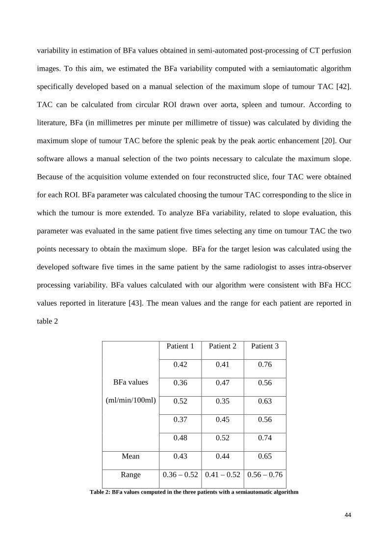
variability in estimation of BFa values obtained in semi-automated post-processing of CT perfusion

images. To this aim, we estimated the BFa variability computed with a semiautomatic algorithm

specifically developed based on a manual selection of the maximum slope of tumour TAC [42].

TAC can be calculated from circular ROI drawn over aorta, spleen and tumour. According to

literature, BFa (in millimetres per minute per millimetre of tissue) was calculated by dividing the

maximum slope of tumour TAC before the splenic peak by the peak aortic enhancement [20]. Our

software allows a manual selection of the two points necessary to calculate the maximum slope.

Because of the acquisition volume extended on four reconstructed slice, four TAC were obtained

for each ROI. BFa parameter was calculated choosing the tumour TAC corresponding to the slice in

which the tumour is more extended. To analyze BFa variability, related to slope evaluation, this

parameter was evaluated in the same patient five times selecting any time on tumour TAC the two

points necessary to obtain the maximum slope. BFa for the target lesion was calculated using the

developed software five times in the same patient by the same radiologist to asses intra-observer

processing variability. BFa values calculated with our algorithm were consistent with BFa HCC

values reported in literature [43]. The mean values and the range for each patient are reported in

table 2

BFa values

(ml/min/100ml)

Patient 1 Patient 2 Patient 3

0.42 0.41 0.76

0.36 0.47 0.56

0.52 0.35 0.63

0.37 0.45 0.56

0.48 0.52 0.74

Mean 0.43 0.44 0.65

Range 0.36 – 0.52 0.41 – 0.52 0.56 – 0.76

Table 2: BFa values computed in the three patients with a semiautomatic algorithm

45

The variability in BFa values is due to the manual selection of the two points necessary to calculate

the maximum slope of the tumour TAC. However, when perfusion CT is used to monitor the effects

of anti-angiogenesis drug therapy (to evaluate vascularisation tumour response), the reproducibility

of the technique must be such that the difference between repeated measurements is small relative

to the magnitude of the therapeutic change in perfusion. For this reason reproducibility of

processing of CT perfusion data is a problem widely debated that limit the clinical application of

this functional image technique. There are a lot of elements that influence reproducibility of

perfusion CT software, independently from the mathematical methods, such as ROI input selection

[44]. We have investigated the BFa intra-observer reproducibility linked to semi-automated

application of the slope method. Obtained results highlighted the necessity to standardise the

selection of starting and ending points in maximum slope assessment. Besides, the analysis of the

curves has evidenced the problem of respiratory misregistration evidenced by the several peaks on

the tumour TAC .

Figure 18: Peaks on TAC. The red and black lines represent two input selection from the operator on the same TAC

Peaks on tumour TAC almost certainly make difficult automatic detection of the maximum slope.

The manual selection of the maximum slope, although introduces variability, seems to be robust to

46

the effect of respiratory misregistration because only one point, basal HU value, is operator

dependent; in fact, the maximum value is undoubtedly identified.

Anyway intra-observer BFa variability in the selection of starting and ending point can be

eliminated if, once the tumour ROI is selected, an automatic algorithm calculates the maximum

slope of TAC curve. Therefore, these preliminary results revealed that new algorithms for an

automatic selection of the maximum slope have to be investigated.

Moreover, in the preliminary approach the problem of TAC fitting has not been considered,

analyzing only the problem of slope computation by manual selection of the line between minimum

and maximum points. It’s clear that processing of TAC can facilitate automatic algorithms for slope

computation.

Therefore, successively, algorithms for an automatic selection of the maximum slope and the effects

of different TAC processing techniques on BFa automatic computation have been investigated.

Some authors have studied the problem of TAC processing in slope method automatic

implementation. Anyway we underline that no specification were declared about algorithms

employed. Bader et alt [36] pointed out that irregularity of the ROI TAC by motion artifacts caused

an increase in the maximum slope of the curves and also represents a cause of perfusion liver

parameter variability. In particular, they concluded that applying slope method to liver, motion

artifacts and the type of data processing influence the assessment of the arterial, portal venous and

total hepatic perfusion but do not influence measurement of HPI. They compare perfusion values

obtained with a fitting procedure (with a gamma fitting) and a smoothing with use of weighted

means algorithm.

Since our preliminary results on the group of three patients have showed that variability in slope

selection can be reduced whit an automatic algorithm, our idea was to test, according to Bader, the

47

effect of different automatic processing on TAC applying slope method [45]. We would have

automatic but reliable algorithms which recognize effectively TAC slope.

As first step, to this particular aim, we proposed a new algorithm to remove outlier points related to

breathing on TAC before the fitting procedure. Then we evaluated the effects of two fitting

procedures applied to tumour TAC: gamma fitting, as suggested by literature [46], and smoothing

spline interpolation. This two automatic procedures were compared with semiautomatic procedure

(manual selection as proposed by Basama). The slope of the line that minimizes the mean square

error was considered as the maximum slope in the selected interval. BFa was calculated in the same

patient with these three different data processing.

The comparison of different TAC processing demonstrated that also applying the same

mathematical model (slope method in our case) perfusion parameter computation is related to the

employed data processing technique. Results about this aspect were obtained applying tested

algorithms to image of eight patients (six males and two females; mean age, 66 years; age range,

52-76).

About data analysis on the axial image displayed by the software, a circular region of interest (ROI)

was drawn around the liver tumour taking care to maintain the ROI within the boundaries of the

mass. A further ROI was drawn around the aorta. Bfa was obtained from automated processing of

the aorta and tumour TAC using the previously described method. Irregular points (i.e. peaks on

TAC) are caused by reproducing a fixed ROI on the temporal images of the same anatomical level.

Because of respiratory misregistration in z direction and x-y plane the selected ROI can include in

the others temporal slices (of the same anatomical region) not only the tumour tissue but also air,

bone or normal liver parenchyma. TAC unreliable data points were excluded with an algorithm that

eliminates the points in which the first derivate is negative or equal to zero. Negative or zero slopes,

until the maximum enhancement of the TAC is reached, are not consistent with our model. This is

in accordance to the physiological assumption of an increase of contrast in the tumour that

48

corresponds to a continuous increment of HU signal (until the maximum enhancement of the TAC

is reached) [12].

After this processing, the TAC of all patients were processed with two methods: a gamma fitting

and a smoothing spline interpolation.

The gamma variate function is expressed as [46]:

31. s� � t� � &�'(bL)�!)!��

*

where K, α and β are fitting parameters.

The gamma variate function has been often used to describe the dispersion of a bolus as it passes

through a series of compartments [46]. For this reason, it is frequently chosen to fit first-pass data in

perfusion studies. Although the gamma variate is an appropriate function to model these situations,

it has several undesirable mathematical properties. Changes in the K, α and β parameters affect not

only the rise and fall times of the function, but also the location and magnitude of the function

maximum. This makes difficult to anticipate how the function will be altered by varying the

parameters [46].

The smoothing spline is a method of smoothing (fitting a smooth curve from a set of noisy

observations) using a spline function. The smoothing spline estimates the function Il (over the class

of twice differentiable functions) that minimize the following equation:

32. ∑ �u> � v�b>��V?>`R T L � vww �b�V,b

where p is a smoothing parameter, controlling the tradeoff between fidelity to the data and

roughness of the function estimate [47]. The fitting procedure was obtained using the "csaps"

MatLab function, where values csaps (x,y,p) return the values of the cubic smoothing spline for the

given data (x,y) and depending on the smoothing parameter p from 0 to 1. In this study, p was the

49

default value chosen by csaps function. This choose is justified by the goodness of visual inspection

of the results in all patients. Spline interpolation doesn't make any assumption about the shape of

the TAC and represents a smoothing procedure that preserves the original shape of tumor liver

pattern [48] [49] reducing undesirable irregularities on the rise of the curve.

Figure 19: Results of different processing on the same raw TAC

Automatic evaluation of maximum slope, by means of first derivate computation, was implemented

over the fitted curves and BFa value was calculated automatically dividing maximum slope by

maximum enhancement value over aorta TAC. BFa was also evaluated for each patient allowing

manual selection on the raw, original TAC (no fitted) of two points required to identify the

maximum slope of the tumor TAC. The slope of the least squares line of the data points (within the

selected interval on TAC) can be assumed as the maximum slope (green line plotted on Fig. 20).

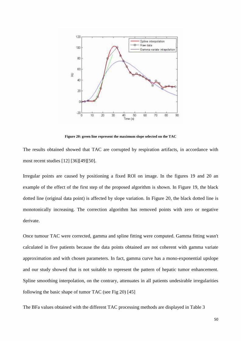
50

Figure 20: green line represent the maximum slope selected on the TAC

The results obtained showed that TAC are corrupted by respiration artifacts, in accordance with

most recent studies [12] [36][49][50].

Irregular points are caused by positioning a fixed ROl on image. In the figures 19 and 20 an

example of the effect of the first step of the proposed algorithm is shown. In Figure 19, the black

dotted line (original data point) is affected by slope variation. In Figure 20, the black dotted line is

monotonically increasing. The correction algorithm has removed points with zero or negative

derivate.

Once tumour TAC were corrected, gamma and spline fitting were computed. Gamma fitting wasn't

calculated in five patients because the data points obtained are not coherent with gamma variate

approximation and with chosen parameters. In fact, gamma curve has a mono-exponential upslope

and our study showed that is not suitable to represent the pattern of hepatic tumor enhancement.

Spline smoothing interpolation, on the contrary, attenuates in all patients undesirable irregularities

following the basic shape of tumor TAC (see Fig 20) [45]

The BFa values obtained with the different TAC processing methods are displayed in Table 3

51

BFa ( spline

fitting)

BFa (gamma fitting) BFa (no fitting with manual

selection)

Patient 1 115.4 - 54.2

Patient 2 120.2 62.4 98.7

Patient 3 119.6 39.3 76.6

Patient 4 85.0 - 43.1

Patient 5 94.6 37.9 52.0

Patient 6 63.1 - 34.3

Patient 7 114.7 - 54.8

Patient 8 80.0 - 51.6

Table 3: BFa values obtained with the different TAC processing in eight patient

BFa computed from spline smoothing TAC interpolation were greater than those obtained with the

other two data processing methods and are more consistent with BFa values reported in literature in

HCC patient [43]. In fact, gamma fitting procedure causes an underestimation of BFa values

because the end data points of TAC are not well approximated. This causes a flattening of the curve

slope of the curve. BFa computed from manual selection were in all patients greater than values

obtained with gamma fitted TAC. However, the estimation of maximum slope, after manual

selection of start and end points, introduces a further element of variability [42].

In conclusion, we can state that fitting procedure and automatic detection of the maximum slope

reduces the variability in assessment of perfusion parameters due to operator. Moreover, both spline

interpolation and gamma fitting procedure are positively influenced by our correction algorithm. In

particular, spline interpolation on corrected data points shows a single up-slope until the maximum

enhancement is reached.

52

However, spline interpolation presented some technical difficulties, for example the automatic

choice of smoothing factor – p value – is particularly difficult in noisy TAC, such as some of those

derived from images acquired in clinical environments during daily practice. Hence, according to

literature, we have considered interesting for research purposes considering also a moving average

(MA - with five coefficient) still in comparison with manual selection of the maximum TAC slope.

When applying the two procedure of fitting (spline and MA filter), the TAC slope is obtained with a

liner fitting of three data points relative to the maximum increment [51].

Since there are not certain guidelines in literature, BFa obtained with manual selection is here

considered the reference.

The results of the comparison are reported in the following table 4.

Patient JK� , manual

(ml/min/100ml)

GRUPPO 1

JK�, spline

interpolation

(ml/min/100ml)

GRUPPO 2

JK�, MA filter

(ml/min/100ml)

GRUPPO 3

1 80.22 127.5100 84.1100

2 77.3300 180.7700 71.7800 3 69.1200 125.3800 70.8600 4 84.1200 149.1400 85.1000 5 75.3300 113.8700 70.5900 6 79.5600 102.5200 77.7300 7 68.3300 117.2900 86.0100 8 120.4600 159.5900 104.5300 9 108.2000 130.2500 99.4300 10 65.5000 103.7700 64.3300 11 84.2300 100.1200 90.3300 12 55.2200 74.6600 49.4700 13 65.6900 167.5600 89.3400 14 49.0900 84.8000 56.9500 15 88.4300 120.1500 86.0500 16 78.2300 102.4100 80.2200 17 81.2300 129.6200 85.1300

Table 4: BFa values computed with different TAC processing. The nonparametric Mann-Whitney U test confirm that results

from group one and three belong from the same population (statistical significance level of 5%)

53

The nonparametric Mann-Whitney U test was used to compare perfusion parameter (BFa) between

the three groups. Null hypothesis is accepted only for group 1 and 3 with a statistical significance

level of 5%.

The results obtained on a larger group of patients confirm that a moving average with fitting of

three data point with maximum increment to compute the slope, represent an automatic and

reliable method to obtain BFa with slope method.

4.4 COMPARISON OF MAXIMUM SLOPE METHOD AND DUAL-INPUT- ONE-

COMPARTMENT-MODEL

The first study about the accord of perfusion CT parameters related to two commercially available

perfusion computed tomographic (CT) software packages demonstrated that there was disagreement

between mathematical model used to estimate tumour vascularity, which indicated the measurement

techniques were not directly interchangeable [52]. Although many researchers have stressed the

clinical usefulness of perfusion CT technique the standardization of analytical method, i.e.

definition of the best mathematical model to compute hepatic perfusion parameter, is still matter of

debate [53][54][55]. Kanda et al [53], comparing hepatic parameter obtained with maximum slope

method (MS), dual input one compartment model (DOCM), and deconvolution method (DM),

conclude that these three analytical method are not interchangeable. DOCM and DM are less

susceptible to extra hepatic system factor, i.e. age , sex, cardiovascular risk, arrival time, transit time

and liver dysfunction or hepatitis. A correlation coefficient of 0,455 (p<0,0001) was calculated to

study the agreement between MS and DOCM. Miyazaki et al [54] reported results about a

simulation study to compare maximum slope and DOCM concluding that MS cause a

underestimation of about 60% with respect to DOCM in BFa computation. In another work the

same author [55] conclude that with venous injection BFa determinated by the MS method was

lower than that obtained by the DOCM method (p<0,05).

54

No author have analyzed the susceptibility of this two methods to noise. So the purpose of our

analysis was to study the effect of noise in BFa computation comparing MS (maximum slope) and

DOCM ( Dual input one compartment model) by simulations.

First, we generated Cl(t) according to DOCM formula setting defined values for K1a, K1p and K2 (

in particular K1a value was set to obtain a corresponding BFa values of 113,4). Ca(t) and Cp(t)

were obtained from images acquired in a clinical perfusion CT study. In this study τa and τp were

assumed to be zero for simplicity [54].

Furthermore, to investigate the effect of statistical noise, we added Gaussian noise to the TAC to

generate signal to noise ratios (SNRs) of 20, 26 and 30. The SNR was given by the standard

deviation of the power of noise free TAC divided by the standard deviation of the noise generated

from normally distribuited random numbers with zero mean and unit variance. Simulation were

performed 10 times for each condition and the mean ad SD of the estimated BFa were calculated.

Results are reported in the following table 5:

Veffsig/Veffn=20

SNR=26

Veffsig/Veffn =10

SNR=20

Veffsig/Veffn=30

SNR=30

BFa (ml/min/100ml) MS 108,4±11,7 145,1±25,1 98,7±11,3

DOCM 130,2±12,7 113,9±17,0 131,0±10,5

Table 5: Bfa values evaluated by MS and DOCM analysis. Results are reported in term of mean and standard deviation of

ten simulation for each SNR conditions. Know value of BFa is 113,4.

Comparison between hepatic perfusion parameters evaluated with the two analytical methods were

performed using Wilcoxon-Mann-Whitney test. P<0,05 was considered significant. BFa

determinate by MS method was lower than that determinate by the DOCM for higher values of

SNR (26 and 30). When the noise is prevalent (SNR=20) slope method algorithm fail and give an

55

increment of BFa values. On the contrary mean value obtained with DOCM have the minor

percentage change from the know BFa value. Our results suggest that our maximum slope

algorithm give bad results in condition of low SNR (percentage change from the know BFa value is

21%). Anyway for other values of SNR (26 and 30) according to literature slope method

underestimate BFa values with respect to DOCM method [54][55].

56

5. SPV INDEX IN CHARACTERIZATION OF ARTERIAL HCC

HYPERVASCULARIZATION

Primitive liver tumour (HCC) diagnosis, assessment and staging are critical because PET (Positron

emission tomography), that represent the gold standard functional technique, is not a useful tool in

the diagnosis and follow up because HCC tumour are not characterized by an increment of glucose.

So, perfusion CT studies in HCC patients are increasingly advocated as a means to assess the grade

of vascularization to evaluate variations in perfusion parameters following locoregional treatments

or antiangiogenic drugs.

One of the specific aim at the start of PhD candidature was to formulate a standardized index, such

as SUV in PET studies, to characterize HCC Hypervascularization. In this Chapter we describe the

theory about the SPV index in HCC and analyze the methodology and the causes of variability that

have to be considered before that a reliable use in clinical practice is possible.

5.1 STANDARDIZED PERFUSION VALUE: HISTORICAL BACKGROUND

SPV index was introduced and applied to lung tumour vascularisation by Miles [56]. This author

underline for the first time that perfusion parameter are largely unaffected by dose, patient weight,

and cardiac output and that a dedicated image acquisition and relatively complex numeric analysis

are required.

SPV index is defined as

33. ��\ 9!9�c

57

where Pt is tumour perfusion and Pwb is mean whole body perfusion. Pwb is defined as Cardiac

Output (CO) divided by patient’s body weight (W).Cardiac output can be evaluated from perfusion

CT images and defined as dose of contrast (D) divided by area under aortic curve (AUC).

The dose of contrast is calculated as below illustrated:

34. � �7�4�( 73 p78 2�5 �� p78 2�5 p78p(8 2� 678 �F�FI � � t3�p 72� ��

"�"Q

�

where K factor represent the calibration factor, i.e. the sensitive of CT system to iodine

concentration.

The SPV is conceptually similar in its derivation to the SUV used to quantify FDG uptake at PET.

The SUV is used to compare FDG uptake in the tissue of interest with the average uptake

throughout the body. Likewise, the SPV is used to compare tissue perfusion with average whole-

body perfusion. The results obtained by Miles showed good correlation between SPV and SUV in

patients with lung tumour.

Other clinical studies have demonstrated that SPV is a useful index to characterize lung and breast

tumor vascularisation [56][57][58], but, for all we know, there are not studies about SPV use in

liver tumor analysis. Moreover there are not study about the consistency of the index and the

problem related to technical aspect.

5.2 SOURCES OF VARIABILITY IN THE USE OF STANDARDIZED PERFUSION VALUE FOR

HCC STUDIES

We believe that could be helpful to employ Standardised Perfusion Value (SPV) in HCC perfusion

studies which has the potential to be a useful non-invasive marker of angiogenesis. However, before

using SPV in clinical practice, we need to verify its reliability. There are different causes of

variability in applying the SPV index, e.g., the technical specifications of the CT system employed

58

and the image processing system. In this chapter we analyse the variability of the BFa estimates and

the variability due to the calibration procedure of the CT system, this with the objective of verifying

how these factors affects SPV values.

5.2.1 MATERIAL AND METHODS

The results are obtained from perfusion MDCT images of seventeen HCC patients. The algorithm,

based on maximum slope method, presented in Chapter 4 was used to compute BFa and then SPV

values.

According to SPV formula proposed by Miles we introduce BFa parameter computed with our

algorithm based on slope method as Pt parameter.

As it can see by the following equation

35. ��\ �k# ��

� #�!�

before the evaluation of SPV, BFa value has to be computed. In this phase, important causes of

variability are slice and ROI selection [59].

5.2.2 ANALYSIS OF BFA VARIABILITY DUE TO ROI MANUAL SELECTION

Four expert radiologists (each with at least two years of experience in CT perfusion) were involved

in the processing of the perfusion image data set for each patient. They were instructed to choose a

single slice, from the perfusion image data set, that best depicted the tumor. Then, a circular ROI

was drawn on the image displayed by the software, this was done in order to include as much of

tumour tissue as possible, still remaining within its boundaries, and to ensure that it did not include

large vessels. Once the slice is selected, different circular ROI of different size and in different

position (respecting the inclusion criteria) can be selected on the same patient. Therefore, to

evaluate the variability related to opera-tor-dependent ROI selection, each radiologist, repeated, on

the same selected slice and a week apart from each other, the input procedure (i.e. ROI position and

dimen-sion) four times on the same image set. For each set of measures (same radiologist and same

59

patient) mean value and standard deviation of BFa values were computed, finally providing the

percentage of variation coefficient as a concise estimation of variability.

5.2.3 CALIBRATION OF THE CT SYSTEM

To evaluate the SPV index, the computation of the calibration K factor of the CT system was

necessary (please see equation 35) . K factor is defined as the slope of the plot of attenuation in HU

vs different con-trast agent concentrations (in milligrams per millimetre) [56]. Therefore, the

calibration procedure aims to deter-mine the calibration K factor that characterizes the linear

relationship between the measured attenuation in HU and the concentration of contrast agent

[60][61]. We have carried out a specific procedure to evaluate the dependence of the K factor from

the position in the CT scan for our CT system.

We performed our calibration procedure with a cylindrical acrylic phantom (Fluke Biomedical)

with five holes. The thickness of the phantom is 15 cm with di-ameter of 32 cm and contains five

pipettes holes (A, B, C, D, E, see Figure 21), one in the centre and four around the perimeter, 90°

apart and 1 cm from the edge. The inside diameter of the holes is 1.31 cm.

Figure 21: Scheme of the phantom used for the calibration procedure.

The phantom includes five acrylic inserts for plugging all the holes not filled with pipettes. Contrast

agent of 400 mg/ml was diluted in physiological saline solution to obtain four different

concentrations (6, 9, 12, 15 mg/ml). These concentrations correspond to physiological con-

centration in abdomen, liver, spleen and major vessels (such as aorta and vena porta) when a

contrast agent bo-lus of 70 ml is injected at a rate of 4 ml/s. Pipettes with five different

60

concentrations of contrast were prepared (0, 6, 9, 12, 15 mg/ml). The scan parameters were the

same used to obtain patients images in our HCC perfusion studies. The phantom was placed on the

scanner table so that the pipettes of contrast agent were parallel to the z-axis of the CT scanner. The

height of the table was adjusted in order to position the phantom at the centre of the CT gantry

(Figure 22).

Figure 22: Example of phantom positioning into the CT gan-try.

Our calibration protocol was based on six configura-tions (P0, PA, PB, PC, PD, PE) corresponding

to different positions of the pipettes in the phantom. The evaluation of K factors in different

configurations aims to esti-mate its dependence on the position in the scan field. In configuration

P0, the five pipettes with different contrast concentrations (0, 6, 9, 12, 15 mg/ml respectively) were

inserted in the five holes (A, B, C, D, E) of the phantom and then scanned simultaneously by means

of a single acquisition using the perfusion protocol scan sequence. In the other configurations, the

five pipettes were in-serted one at a time in the same hole (i.e. A correspond-ing to PA, B to PB, C

to PC, D to PD and E to PE con-figuration), and the others holes were filled with acrylic inserts.

Therefore, for these configurations, five scans were necessary, each of them with a different

61

contrast agent concentration in the pipette, in order to estimate the K factor corresponding to every

position. Since each TC scan provides 8 images, 8 K factors and their mean and standard deviation

were computed for each configuration. To determine the K factor, regions of interest (ROI) were

located by the operator on images in correspondence with each pipette containing contrast agent.

The dimensions of the ROI were chosen as large as possible and avoiding partial volume effects and

air bubbles generated during preparation of the solutions. For each contrast agent concentration, the

mean values of gray levels (HU units) in each ROI were obtained in the different images. The slope

of a linear least square fit of the five points (HU vs milligrams per milliliter) gave the calibration

factor.

5.2.4 RESULTS

Results obtained about the estimation of variability in BFa evaluation are shown in Table 6.

Table 6: Results obtained by the four radiologists in BFa estimation shown as average (µ), standard deviation (σ) and coeffi-

cient of variation in percentage (RSD)

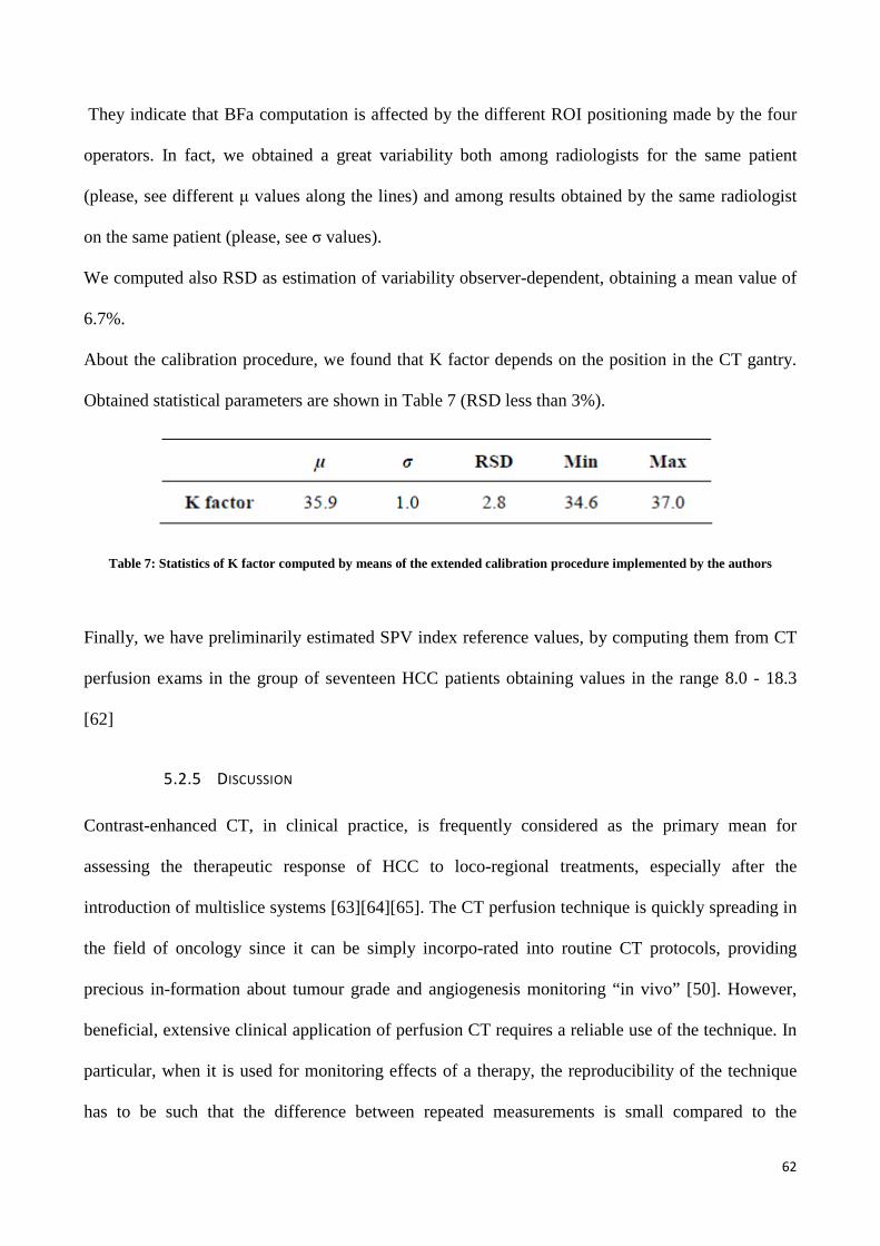
62

They indicate that BFa computation is affected by the different ROI positioning made by the four

operators. In fact, we obtained a great variability both among radiologists for the same patient

(please, see different µ values along the lines) and among results obtained by the same radiologist

on the same patient (please, see σ values).

We computed also RSD as estimation of variability observer-dependent, obtaining a mean value of

6.7%.

About the calibration procedure, we found that K factor depends on the position in the CT gantry.

Obtained statistical parameters are shown in Table 7 (RSD less than 3%).

Table 7: Statistics of K factor computed by means of the extended calibration procedure implemented by the authors

Finally, we have preliminarily estimated SPV index reference values, by computing them from CT

perfusion exams in the group of seventeen HCC patients obtaining values in the range 8.0 - 18.3

[62]

5.2.5 DISCUSSION

Contrast-enhanced CT, in clinical practice, is frequently considered as the primary mean for

assessing the therapeutic response of HCC to loco-regional treatments, especially after the

introduction of multislice systems [63][64][65]. The CT perfusion technique is quickly spreading in

the field of oncology since it can be simply incorpo-rated into routine CT protocols, providing

precious in-formation about tumour grade and angiogenesis monitoring “in vivo” [50]. However,

beneficial, extensive clinical application of perfusion CT requires a reliable use of the technique. In

particular, when it is used for monitoring effects of a therapy, the reproducibility of the technique

has to be such that the difference between repeated measurements is small compared to the

63

variability due to therapeutic changes [50]. At the moment, there are encouraging preliminary

findings about reproducibility of the methodology and intra- and inter-observer variability but they

regard only some body regions [66], not including the liver.

Software packages involving SPV computation are considered as advantageous in oncological

applications [50], but we believe that the first application of SPV index to liver tumor is described

here. At the best of our knowledge, in fact, there are no studies about SPV application in HCC

patients, although perfusion CT studies are widely used in characterization of liver tumor. We

believe that SPV index could be very helpful in liver tumor studies, nevertheless its application in

clinical practice requires a preliminary evaluation of its reliability. In this study we wanted to

provide details about some limitations of this technique.

Important is, for example, the variability in SPV computation. SPV index, normalised respect to CO

and patient’s weight was proposed by Miles [56] to reduce variability relative to these parameters.

However, as can be seen from Equation (35), there is still variability due to K and BFa calculation.

BFa computation is mainly related to the subjective positioning of the ROI done by a specific

operator. Our results are in accordance with other works in which is reported the variability of the

perfusion parameter, related to the processing analysis of perfusion image [66][67].

The positioning of the ROI consists in manually drawing a circular ROI along tumor margins so to

allow the software to quantify perfusion values within it. It is crucial that the ROI is placed within

tumor margins in all perfusion scan images. By consequence, all images of the study should be

carefully analyzed, preferably in cine-loop modality, to ensure that the ROI does not ex-tend

beyond tumour margins and does not include vessels, air or surrounding adipose tissue in any of

them. However, this procedure does not solve problems relative to patient movements during the

time of acquisition. In fact, it is very difficult to choose a ROI that remains still on the tumor in each

different image. The solution could be the selection of a different ROI for each image; however, this

procedure can be boring for the operator, is time consuming and could introduce other sources of

variability. Therefore, generally (as done also for this research work), once drawn a ROI, it should

64

be placed in the same position on all the temporal images of the same anatomical level [45].

Because of respiratory misregistration, which represents an important source of error, as reported

also by other authors, it is possible that the selected ROI can include, in some slices, not only the

tumor but also air, bone or normal liver parenchyma.

The calibration of CT systems is a necessary procedure, being the K factor a parameter included in

the formula for computing the SPV.

Calibration factor depends on the specific CT system and on the acquisition parameters (KVp, mAs,

kernel reconstruction) and changes over time. Some authors [68] proposed to compute K factor for

each patient. Others [60] stated that it would be prudent to calibrate the CT system on the same day

for each quantitative contrast- enhanced study.

However, we consider this recommendation a limit in clinical practice, because of the time needed

to calibrate the system. Therefore, in order to verify if it is possible to avoid a complex calibration

procedure, we estimated the contribution of K factor variability to the variability of SPV index

respect to the variability due to BFa evaluation.

Calibration factor variance, due to the position in the gantry, resulted less than BFa variability

(which is more than the double). So, we concluded that, if the daily calibration is preferred, a

simplified protocol, which neglects the dependence of K factor from the position, may be utilised.

Otherwise, also according to literature, we advice, to keep it on the safe side, that calibration

procedure should be repeated about every two weeks for a specific CT system, before that the

amount of K factor variation, reported in literature [60], becomes comparable with variability due to

BFa estimation, found in our results.

Finally, concerning values of SPV index, we evaluated them in seventeen patients in order to

preliminarily verify the accordance between obtained results and the theoretical hypothesis that,

being HCC characterised by a higher vascularisation respect to other kinds of tumours, it should

show higher SPV values. We retain to have obtained interesting results even though our patients

number was not so large and a direct comparison with the SPV values in other organs was not

65

possible. In fact, as expected, we found high SPV values (8.0 - 18.3) that characterize the hyper-

vascularised HCC lesion, respect to lung (range 1.13 - 10.36) [56] [57] and breast tumour (range 2.5

- 5.9) [58].

5.2.6 CONCLUSION

The application of SPV index in HCC tumor could have a great potential in the management of

HCC patients. However, to ensure the reliability of SPV perfusion index, it is advisable to use

always the same acquisition protocol and to calibrate the CT system with the same measurements

conditions at least every two weeks. Nevertheless, we have demonstrated that this aspect can be

neglected until the intrinsic variability of perfusion parameter computation will be reduced.

In conclusion, we suggest the use of SPV index since CT perfusion provides qualitative assessment

of vascularisation and therapeutic effects whereas a quantitative evaluation can be more useful. The

use of SPV Index could be a feasible and non-invasive tool in the management and follow up of

TACE/TAE, PEI, radiofrequency ablation and radioembolization treatment in HCC patients. This

treatments are the most suited in patients with non surgical lesions in early, intermediate and

advanced stage [69]. The response to these loco-regional treatments may be evaluated by comparing

the difference in SPV values pre- and post-treatment.

The results of this work represent, in our opinion, an important step in the evaluation of the use of

SPV index in liver tumor perfusion studies. However, we aware that the main limitation of our

study is the small volume of coverage related to the image CT system. This volume is limited along

the z-axis by the number of CT detectors used (e.g. 2.4 cm for our 16-slice CT system). Anyway, 16

slices CT systems are still widely spread and applied in the follow up of HCC patients [17].

66

6. PERFUSION MAPS

We have seen that evaluation of quantitative parameters about tumor perfusion, such as blood flow,

by CT perfusion is gaining acceptance in clinical applications. “ROI based” analysis can be

considered the gold standard technique to derive quantitative parameters, although it does not allow

to depict the heterogeneous vascularisation of tumor tissue. On the contrary, “pixel by pixel”

analysis, which has this potentiality, leads only to qualitative depiction of tumor perfusion by means

of colour scale since still lacks of robust processing methods. In this chapter, we propose an

algorithm for parametric estimation (pixel by pixel) of BFa values and used it for the analysis of a

group of seventeen patients with primary liver tumour. Then, we compared obtained BFa values

with those estimated by a “ROI based”approach, by using the same image processing, to investigate

the reliability of parametric maps computed with the algorithm developed. Then an analysis by a

“map based” approach was conducted to compare the performances of pixel by pixel MS and

DOCM algorithm.

6.1 ROI APPROCH VS PIXEL BY PIXEL APPROACH: THE VALUE OF PERFUSION MAP

In literature, the first techniques, used for quantitative perfusion evaluation, were based on analysis

of average HU variation in regions of interest (ROIs), identified manually on the functional images

[10][27][30]. However, perfusion may be heterogeneously distributed and information regarding the

differences may in this way be lost. In order to obtain more detailed information about perfusion,

several attempts have been made to apply the kinetic calculations to individual pixel data and the

generated distribution map is often referred to as a parametric image [22][41][70]. Nevertheless,

parametric maps had initially only a qualitative value, because they were used just to help the

radiologist in ROI positioning without validation of employed processing, so that their reliability as

tool for quantitative estimation of perfusion parameters is still matter of debate. Pixel by pixel

67

analysis leads to high variance of the estimates and variance reduction by posterior spatial

averaging produce variable results.

As we have seen in chapter 3, pixel TAC is noisier that ROI TAC because the effect of by photon

noise. When generating TAC from very small regions or individual pixel, photon noise, in fact,

becomes an important consideration. Random variations in photon numbers cause variability in

measured attenuation values and hence, errors in the calculated perfusion values [20]. The problem

of liver perfusion CT map processing is minimally addressed by other authors at the best of our

knowledge. However some authors have published detail about parametric mapping algorithm in

liver and myocardial perfusion MRI studies [51][71] and cerebral perfusion CT studies. When

processing pixel TACs we have different problem than ROI TAC processing. First of all we have

applied gamma fitting to pixel TAC. Our results showed that this fitting is not applicable because of

the height noise. Gamma model, infact, is adapted to represent the first part (upslope) of liver TACs

and represent the dynamic phenomenon of contrast input with a single upslope. The experimental

analysis of pixel liver and tumour TAC have demonstrated that there are two upslope related to

arterial and portal phase. Gamma equation is not a good model for the pixel data. Spline

interpolation is always applicable to pixel TAC but the problem is that pixel TAC are noisier than

ROI TAC and the algorithm to remove outlier (proposed and applied to ROI TAC) don’t give good

results. Pixel spline interpolation is more affected by the noise than TAC spline interpolation and

this cause map of poor quality that not simple allow ROI positioning.

68

Figure 23: BFa map obtained with slope method algorithm

Moreover quantitative value obtained with spline fitting map overestimate arterial Blood Flow in

primitive liver tumours (mean value in seventeen HCC patient is 320 ml/min/100ml). Our results

suggest that a more reliable algorithms have to be investigated to obtain quantitative and qualitative

map of BFa in liver tumour.

In this thesis we introduce an algorithm for parametric estimation (pixel by pixel) of BFa values

with slope method. Then, because ROI based approach can be considered the “gold standard” for

quantitative values, a comparison with our proposed algorithm is made to assess the reliability.

Figure 24 : Flow chart of algorithm used to obtain BFa map according to slope method

An analysis of correlation between perfusion parameters computed with a traditional ROI based

approach and the values computed by means of a pixel

image processing technique) is presented.

According to literature [72], before analysis, a double threshold was imposed on the image set to

exclude air and bone (only pixels include

perfusion image sequence of the liver tumour, the pixel values at each specific pair of coordinates in

all the successive images were extracted to obtain a one dimensional HU array (1

represents the pixel-TAC. This

moving-average filter), to reduce noise contribute. An array of differences (1

represents the contrast time variation, was then computed by the 1

positive element in the 1-D-diff array corresponds to the maximum contrast positive variation.

Three consecutive data points in the 1

largest element identified in 1-D



values computed by means of a pixel-by-pixel map approach (using the same

image processing technique) is presented.

before analysis, a double threshold was imposed on the image set to

exclude air and bone (only pixels included in the range -50÷200 HU were analyzed).


all the successive images were extracted to obtain a one dimensional HU array (1

TAC. This pixel-TAC was smoothed [36] with an average filter (5th

average filter), to reduce noise contribute. An array of differences (1

represents the contrast time variation, was then computed by the 1-D-array. Of course, the largest

diff array corresponds to the maximum contrast positive variation.

Three consecutive data points in the 1-D-array, centered around the element corresponding to the

D-diff, were then considered. The three consecutive points were

69



pixel map approach (using the same

before analysis, a double threshold was imposed on the image set to

50÷200 HU were analyzed). For each CT


all the successive images were extracted to obtain a one dimensional HU array (1-D-array), which

with an average filter (5th-order

average filter), to reduce noise contribute. An array of differences (1-D-diff), which

ray. Of course, the largest

diff array corresponds to the maximum contrast positive variation.

array, centered around the element corresponding to the

ff, were then considered. The three consecutive points were

70

fitted using a linear curve fitting model. The slope of the regression line was considered as the

maximum slope of the pixel-TAC. The procedure was repeated for calculating the up-slope of each

pixel over the whole image. Thus, the image series was reduced to a single image (a parametric

map) where each pixel value corresponds to the maximum up-slope of the TAC at that coordinates.

According to Miles [50], dividing the parametric map by the maximum value of aorta-TAC

(computed in a traditional way), we obtained the BFa parametric map. To compute BFa mean,

variance and maximum values, a circular ROI was placed on the map in correspondence of the

tumour region. The ROI was chosen to include the largest possible part of the tumour tissue, while

remaining within its boundaries, and to ensure that it did not include large vessels. The same ROI

choose for the map approach was drawn on the image of the tumour in the CT perfusion images.

The mean of HU values inside the ROI were computed for each slice of the sequence to compute a

mean tumor TAC. The processing used for the map approach was applied to this mean curve to

obtain BFa values. BFa values computed using the map approach were plotted against BFa values

computed by means of the ROI approach. The regression line shows the agreement between these

values (Goodness of fit: SSE: 194.1 R-square: 0.90 Adjusted R-square: 0.89 RMSE: 3.6).

Figure 25: Correlation analysis between BFa values obtained with “ROI based” and “map based” approach

71

Anyway, the values obtained from the map were on average higher than those obtained from the

ROI approach. That could probably due to the greater effect of the noise on the processing of the

pixels-TAC. In fact, the presence of breathing, even if gentle, during dynamic imaging, did cause

local errors in BFa estimation due to the movement of small structures between consecutive time

slices, especially around the time of contrast arrival. This effect is a minor problem for ROI

approach, probably for the effect of the mean operation inside the ROI. The R value obtained

supports the idea that the use of an adequate processing permits to obtain reliable BFa maps

compared with the ROI approach. Assessment of quantitative parameters by CT perfusion maps is

still an open issue although the wide spread of perfusion technique in clinical practice. We have

developed and tested in a group of 17 HCC patients an algorithm based on slope method to obtain

perfusion maps . The results are in accordance with those obtained with a traditional ROI approach,

using the same image processing algorithm. This suggests that the developed algorithm could give

useful quantitative information about tumour heterogeneous hypervascularisation.

Figure 26: A BFa map obtained with the developed slope method algorithm

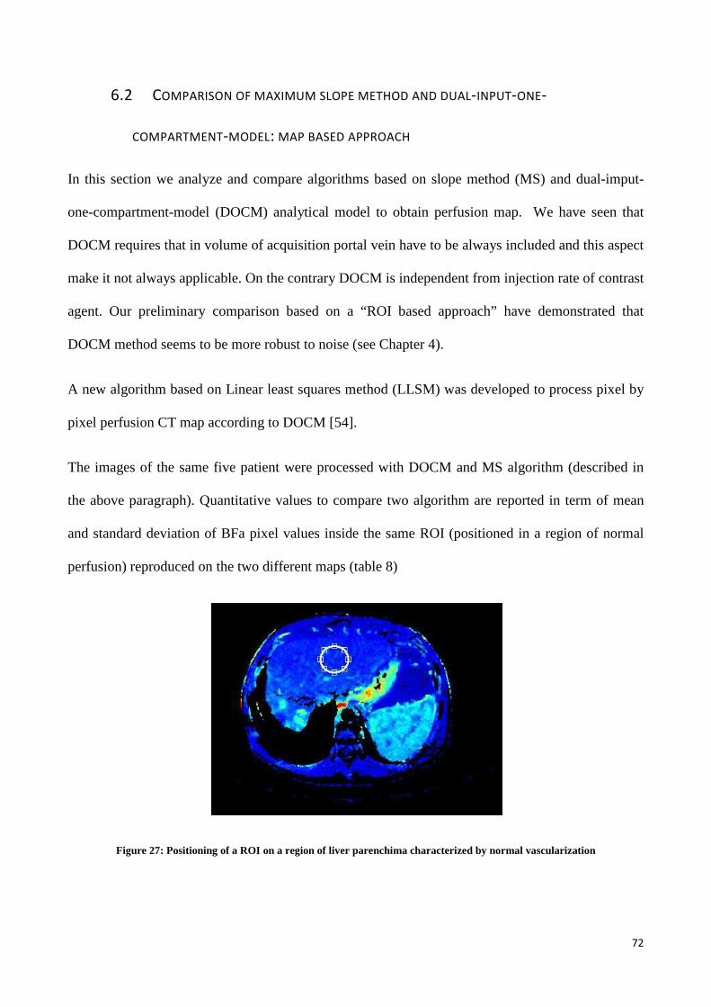
72

6.2 COMPARISON OF MAXIMUM SLOPE METHOD AND DUAL-INPUT-ONE-

COMPARTMENT-MODEL: MAP BASED APPROACH

In this section we analyze and compare algorithms based on slope method (MS) and dual-imput-

one-compartment-model (DOCM) analytical model to obtain perfusion map. We have seen that

DOCM requires that in volume of acquisition portal vein have to be always included and this aspect

make it not always applicable. On the contrary DOCM is independent from injection rate of contrast

agent. Our preliminary comparison based on a “ROI based approach” have demonstrated that

DOCM method seems to be more robust to noise (see Chapter 4).

A new algorithm based on Linear least squares method (LLSM) was developed to process pixel by

pixel perfusion CT map according to DOCM [54].

The images of the same five patient were processed with DOCM and MS algorithm (described in

the above paragraph). Quantitative values to compare two algorithm are reported in term of mean

and standard deviation of BFa pixel values inside the same ROI (positioned in a region of normal

perfusion) reproduced on the two different maps (table 8)

Figure 27: Positioning of a ROI on a region of liver parenchima characterized by normal vascularization

73

Table 8: BFa values computed with MS and DOCM algorithms. µ and σ are respectively the mean and the standard

deviation of pixel values inside the ROI

Because the ROIs were positioned in a region of liver parenchyma characterized by uniform

vascularisation to compare the two algorithm SNR was defined as the ratio of µ and σ (table 9)

Table 9: Results reported in term of SNR

Patient BFa

MS(ml/min/100ml)

BFa

DOCM(ml/min/100ml)

µ σ µ σ

N° 1 39,45 5,210 31,68 30,32

N° 2 44,87 13,60 28,55 29,56

N° 3 62,32 7,684 27,32 18,77

N° 4 57,16 6,881 26,36 25,86

N° 5 64,94 15,86 17,63 12,70

Patient SNR - MS SNR - DOCM

µ/σ 10log µ/σ µ/σ 10log µ/σ

N° 1 7,572 8,792 1,045 0,191

N° 2 3,299 5,184 0,966 -0,150

N° 3 8,110 9,090 1,456 1,632

N° 4 8,307 9,194 1,019 0,082

N° 5 4,095 6,123 1,388 1,434

74

The analysis of results demonstrate that SNR values associated to MS are lower that those

calculated for DOCM. It means that slope method algorithm is preferable to compute quantitative

BFa maps.

Figure 28: BFa map computed on the same patient with MS and DOCM algorithms

The analysis of BFa maps showed that even from the qualitative point of view the MS method

(image on the left) is more reliable: in the right image (DOCM) the tumour is not visible and the

spleen appears to be perfused as the liver parenchyma in the arterial phase (in opposition with the

physiological processes of abdominal perfusion).

75

7. CONCLUSION

Improved therapeutic options for hepatocellular carcinoma place greater demands on surveillance

tests for liver disease. Existing diagnostic imaging techniques provide limited evaluation of tissue

characteristics beyond morphology; perfusion CT imaging of the liver has potential to improve this

shortcoming. Perfusion parameters can be obtained applying mathematical model to TAC, i.e.

contrast agent evolution over the time in a specific ROI positioned on the images. However, there

are still some difficulties for an accurate and absolute quantification of perfusion parameters due,

for example, to algorithms employed, to tracer kinetic modelling methods, to patient’s weight and

cardiac output, to the acquisition system.

In this thesis, new parameters or methods of interpretation and alternative methodologies about liver

perfusion CT are presented in order to further investigate the potential and the limits of this

technique.

Firstly analysis were made to assess the variability related to the mathematical model used to

compute BFa values. Results were obtained implementing algorithms based on MS and DOCM.

Statistical analysis on simulated data demonstrated that the two methods are not interchangeable

regardless of the signal to noise ratio. Anyway slope method is the most used model to obtain

perfusion parameters and allow to compute BFa values always when portal vein is not visible in

perfusion CT scan.

Then variability related to TAC processing in the application of slope method is analyzed. Our aim

was to find an automatic and reliable algorithm to compute TAC maximum slope after TAC

processing. A fifth order smoothing with an automatic algorithm (that calculate the straight line

fitting three points corresponding to TAC maximum increase) give the best results compared with

manual selection.

76

Variability related to the patient, to the acquisition system and to the operator which select the ROI

on the images are than analyzed. The consistency of SPV index was evaluated and a simplified

calibration procedure was proposed. The application of SPV index allow to identify a clinical range

to characterize HCC. At the end the quantitative value of perfusion map was analyzed. ROI

approach and map approach provide related values of BFa and this means that pixel by pixel slope

method algorithm give reliable quantitative results. Also in pixel by pixel approach MS algorithm

present results uncorrelated with DOCM. Moreover DOCM method give quantitative results

characterized by lower SNR value.

In conclusion, although it presents some limitation in the post-processing analysis, liver perfusion

CT techniques are becoming an important tool in the medical research and clinical practice. The

development of new automatic algorithm for a consistent computation of BFa and the analysis and

definition of simplified technique to compute SPV parameter, would improve the clinical and

scientific information provided by liver perfusion CT analysis.

77

REFERENCES

1. Pandharipande PV, Krinsky GA et al. Perfusion Imaging of the Liver: Current

Challenges and Future Goals. Radiology 2005; 234: 661-673.

2. Folkman J, P Cole et al. Tumor behavior in isolated perfused organs: in vitro

growth and metastases of biopsy material in rabbit thyroid and canine intestinal

segment. Ann Surg 1966; 164:491–502.

3. Folkman J. The role of angiogenesis in tumor growth. Semin Cancer Biol 1992;

3:65–71.

4. Folkman J. Role of angiogenesis in tumor growth and metastasis. Semin Oncol

2002; 29:15–18.

5. Park YN, Yang CP et al. Neoangiogenesis and sinusoidal “capillarization” in

dysplastic nodules of the liver. Am J Surg Pathol 1998; 22:656–662.

6. Roncalli M, Roz E et al. The vascular profile of regenerative and dysplastic

nodules of the cirrhotic liver: implications for diagnosis and classification.

Hepatology 1999; 30:1174–1178.

7. Krinsky GA, Theise ND et al. Dysplastic nodules in cirrhotic liver: arterial phase

enhancement at CT and MR imaging: a case report. Radiology 1998; 209:461–

464.

8. Krinsky GA, Zivin SB et al. Low-grade siderotic dysplastic nodules:

determination of premalignant lesions on the basis of vasculature phenotype.

Acad Radiol 2002; 9:336–341.

9. Park YN, Kim YB, et al. Increased expression of vascular endothelial growth

factor and angiogenesis in the early stage of multistep hepatocarcinogenesis.

Arch Pathol Lab Med 2000; 124:1061–1065.

78

10. Zhao J, Hu J et al. Vascular endothelial growth factor expression in serum of

patients with hepatocellular carcinoma. Chin Med J(Engl) 2003; 116:772–776.

11. Chao Y, Li CP et al. Prognostic significance of vascular endothelial growth

factor, basic fibroblast growth factor, and angiogenin in patients with resectable

hepatocellular carcinoma after surgery. Ann Surg Oncol 2003; 10: 355–362.

12. K. A. Miles. Perfusion CT for the Assessment of Tumour Vascularity: Which

Protocol?. The British Journal of Radiology 2003; 761(1):S36-S42.

13. D. V. Sahani, N. Holalkere et al. Role of Perfusion CT in Monitoring Anti-

Angiogenic Response in Patients with Advanced Hepatocellular Carcinoma.

Contrast Media and Molecular Imaging 2006; 1 (2): 72-72.

14. G. Chen, D.-Q. Ma et al. Computed Tomography Perfusion in Evaluating the

Therapeutic Effect of Transarterial Chemoembolization for Hepatocellular

Carcinoma. World Journal of Gastroenterology 2008; 14 (37): 5738-5743.

15. Z. Kan, S. Phongkitkarun, et al. Functional CT for Quantifying Tumor Perfusion

in Antiangiogenic Therapy in a Rat Model. Radiology 2005; 237 (1): 151-158.

16. Z. Kan, S. Kobayashi et al. Functional CT Quantification of Tumor Perfusion

after Transhepatic Arterial Embolization in a Rat Model. Radiology 2005; 237

(1): 144-150.

17. Sahani DV, Holalkere NS et al. Advanced hepatocellular carcinoma: CT

perfusion of liver and tumor tissue--initial experience. Radiology 2007;

243(3):736-43.

18. Byung Ihn Choi. Advances of Imaging for Hepatocellular Carcinoma. Oncology

2010;78 (Suppl. 1):46-52.

19. Ippolito, D., Sironi et al. Perfusion computed tomographic assessment of early

hepatocellular carcinoma in cirrhotic liver disease: initial observations. Journal of

computer assisted tomography 2008; 32(6): 855-858.

79

20. K. A. Miles, M. P. Hayball et al. Functional images of hepatic perfusion obtained

with dynamic CT. Radiology 1993; 188:405–411.

21. M. J. Blomley, R. Coulden et al. “Liver perfusion studied with ultrafast CT”. J

Comput Assist Tomogr 1995; 19:424–433.

22. Y. Tsushima, S. Funabasama et al. Quantitative perfusion map of malignant liver

tumors, created from dynamic computed tomography data. Acad Radiol 2004;

11: 215-223.

23. H. F. Yang, Y. Du et al. Perfusion computed tomography evaluation of

angiogenesis in liver cancer. Eur Radiol 2010; 20: 1424–1430.

24. A. Komemushi, N. Tanigawa et al. CT perfusion of the liver during selective

hepatic arteriography: pure arterial blood perfusion of liver tumor and

parenchyma”. Radiat Med 2003; 21: 246-251

25. Peters AM, Brown J. et al. Non- invasive measurement of renal blood flow with

99mTc DTPA: comparison with radiolabelled microspheres. Cardiovasc Res

1987;21(11):830-4.

26. Peters AM, Gunasekera RD et al. Noninvasive measurement of blood flow and

extraction fraction. Nucl Med Commun 1987;8(10):823-37.

27. Miles KA. Measurement of tissue perfusion by dynamic computed tomography.

Br J Radiol 1991;64(761):409-12.

28. Miles KA, Hayball MP et al. Functional images of hepatic perfusion obtained

with dynamic CT. Radiology 1993;188(2):405-11.

29. Miles KA, Hayball MP et al. Measurement of human pancreatic perfusion using

dynamic computed tomography with perfusion imaging. Br J Radiol 1995;

68(809):471-5.

30. Blomley MJ, Coulden R et al. Liver perfusion studied with ultrafast CT. Journal

of Computer Assisted Tomography 1995; 19(3):424-433.

80

31. Tsushima Y, Blomley MJK et al. Measuring portal venous perfusion with

contrast-enhanced CT: comparison of direct and indirect methods. Acad Radiol

2002;9:276–82.

32. Materne R, Van Beers BE et al. Non-invasive quantification of liver perfusion

with dynamic computed tomography and a dual-input one-compartmental model.

Clin Sci (Lond) 2000; 99(6):517-25.

33. Van Beers BE, Leconte I et al. Hepatic perfusion parameters in chronic liver

disease: dynamic CT measurements correlated with disease severity. AJR Am J

Roentgenol 2001; 176: 667–73.

34. Cuenod CA, Leconte I et al. Deconvolution technique for measuring tissue

perfusion by dynamic CT: application to normal and metastatic liver. Acad

Radiol. 2002; 9(1):S205-11.

35. Axel L. Cerebral blood flow determination by rapid-sequence computed

tomography. Radiology 1980; 137:679–686.

36. Bader TR, Grabenwöger F et al. Measurement of hepatic perfusion with dynamic

computed tomography: assessment of normal values and comparison of two

methods to compensate for motion artifacts. Invest Radiol. 2000; 35(9):539-47.

37. Roland Materne, Bernard E. et al. Hepatic perfusion after liver transplantation:

non invasive measurement with dynamic single-section CT. Clinical Science

2000. 99: 517–525.

38. Adri¨enne Mendrik, Evert-jan Vonken et al. Noise filtering in thin-slice 4D

Cerebral CT Perfusion scans. Proc. of SPIE 2010; 7623

39. Xin Liu, Andrew N. Primak et al. Quantitative evaluation of noise reduction

algorithms for very low dose renal CT perfusion imaging. Proc. of SPIE 2009;

7258.

81

40. H. Bruder, R. Raupach et al. Spatio-temporal filtration of dynamic CT data using

diffusion filters. Proc. of SPIE 2009; 7258.

41. Yoshito Tsushima, Shintaro Funabasama et al. Development of Perfusion CT

software for personal computers. Academic Radiology 2002; 9 (8): 922–926

42. M. D'Anto, M. Cesarelli et al. Perfusion CT of the liver: slope method analysis.

Proc. of GNB Conference, Torino, 2010.

43. Zhong, W. J. Wang et al. Clinical application of hepatic CT perfusion. World J

Gastroenterol 2009; 15(8): 907-911.

44. Pina C. Sanelli, Gregory Nicola et al. Reproducibility of Postprocessing of

Quantitative CT Perfusion Maps. AJR 2007; 188:213-218.

45. M. D’Antò, M.Cesarelli et al. Study of different Time Attenuation Curve

processing in Liver CT Perfusion. Proc. of 10th IEEE International Conference

on Information Technology and Applications in Biomedicine (ITAB), Corfù

(Greece) 2010.

46. M. T. Madsen. A simplified formulation of the gamma variate function. Phys.

Med. Bid. 1992; 1: 1597-1600.

47. M. Unser, Splines: A perfect Fit for Signal and Image Processing. IEEE signal

processing magazine 1999; 16 (6): 22-38

48. T. R. Bader, A. M. Hemeth et al. Hepatic Perfusion after Liver Transplantation:

Noninvasive Measurement with Dynamic Single-Section CT. Radiology 1998,

209: 129-134.

49. K. A. Miles. Functional computed tomography in Oncology. Eur J Cancer 2002;

38 (16) : 2079-84.

50. K.A. Miles, M.R. Griffiths. Perfusion CT: a worthwhile enhancement? BrJ

Radiol 2003; 76: 220-31.

82

51. Chun Ruan, Scott Yang et al. First-Pass Contrast-Enhanced Myocardial

Perfusion MRI Using a Maximum Up-Slope Parametric Map. IEEE Transactions

on Information Technology in Biomedicine 2006; 10 (3): Page 574-580.

52. Vicky Goh, Steve Halligan et al. Quantitative Tumor Perfusion Assessment with

Multidetector CT: Are Measurements from Two Commercial Software Packages

Interchangeable? Radiology 2007; 242: 777-782.

53. Tomonori Kanda, Takeshi Yoshikawa et al. CT hepatic perfusion measurement:

comparison of three analytic methods. European Journal of Radiology 2012; 81

(9):2075–2079.

54. S. Miyazaki, K. Murase et al. A quantitative method for estimating hepatic blood

flow using a dual-input single-compartment model. British Journal of Radiology

2008; 81:790-800.

55. Masaya Miyazaki, Yoshito Tsushima et al. Quantification of hepatic arterial and

portal perfusion with dynamic computed tomography: comparison of maximum-

slope and dual-input one-compartment model methods. Japanese Journal of

Radiology 2009; 27(3): 143-150.

56. Kenneth A. Miles, Matthew R. Griffiths et al. Standardized Perfusion Value:

Universal CT Contrast Enhancement Scale that Correlates with FDG PET in

Lung Nodules. Radiology 2001; 220: 548-553.

57. K. A. Miles, M. R. Griffiths et al. Blood Flow-Metabolic Relationships are

Dependent on Tumour Size in Non-Small Cell Lung Cancer: A Study Using

Quantitative Contrast-Enhanced Computer Tomography and Positron Emission

Tomography. European Journal of Nuclear Medicine and Molecular Imaging

2005; 33 (1): 22-28.

58. Ashley M Groves, Gordon C Wishart, et al. Metabolic-Flow Relationships in

Primary Breast Cancer: Feasibility of Combined PET/ Dynamic Contrast-

83

Enhanced CT. European Journal of Nuclear Medicine and Molecular Imaging

2009; 36 (3): 416-421.

59. V. Goh, S. Halligan et al. Quantitative Assessment of Colorectal Cancer Tumor

Vascular Parameters by Using Perfusion CT: Influence of Tumor Region of

Interest. Radiology 2008; 247 (3): 726-732.

60. K. A. Miles, H. Young et al. Quantitative Contrast-Enhanced Computed

Tomography: Is There a Need for System Calibration? European Radiology

2007; 17 (4): 919-926.

61. M. J. Siegel, B. Schmidt et al. Radiation Dose and Image Quality in Pediatric

CT: Effect of Technical Factors and Phantom Size and Shape. Radiology 2004;

233 (2): 515-522.

62. Michela D’Antò, Mario Cesarelli et al. Sources of Variability in the Use of

Standardized Perfusion Value for HCC Studies. OJMI 2012; 2 (2): 33-40

63. F. Fiore, P. Vallone et al. Levovist-Enhanced Doppler Sonogra-phy Versus Spiral

Computed Tomography to Evaluate Response to Percutaneous Ethanol Injection

in Hepato-cellular Carcinoma. Journal of Clinical Gastroenterology 2003; 36 (1):

63-67.

64. H. K. Lim, D. Choi et al. Hepatocellular Carcinoma Treated with Per-cutaneous

Radio-Frequency Ablation: Evaluation with Follow-Up Multiphase Helical CT.

Radiology 2001; 221 (2): 447-454.

65. I. R. Kamel, E. Liapi et al. Multidetector CT of Hepatocellular Carcinoma. Best

Practice & Re-search Clinical Gastroenterology 2005; 19 (1): 63-89.

66. D. Fiorella, J. Heiserman et al. Assessment of the Reproducibility of

Postprocessing Dy-namic CT Perfusion Data. American Journal of Neuro-

radiology 2004; 25 (1): 97-107.

84

67. V. Goh, S. Halligan, et al. Quantitative Assessment of Colorectal Cancer

Perfusion Using MDCT: Inter- and Intraobserver Agree-ment. American Journal

of Roentgenology 2005; 185 (1): 225-231.

68. K. Takanami, S. Higano et al. Validation of the Use of Calibration Factors

between the Iodine Concentration and the Computed Tomography Number

Measured outside the Objects for Estimation of Iodine Concentration inside the

Objects: Phantom Experiment. Radiation Medicine 2008; 26 (4): 237-243.

69. R. Wong, C. Frenette. Management of Hepatocellular Carcinoma: An Update

Hepatology 2011; 53 (3): 16-24.

70. Petralia G., Preda L. et al. CT perfusion in solid-body tumours. Part I: technical

issues Radiol med 2010; 115:843–857.

71. Zavaljevski Aleksandar, Holland Scott K. Et al. Multilevel computed

hemodynamic parameter maps from dynamic perfusion MRI. IEEE Transactions

on Instrumentation and Measurement 1999; 48 (3): 711- 720.

72. Y. Tsushima, Y. Unno et al. Measurement of human hepatic and splenic

perfusion using dynamic computed tomography: a preliminary report. Comput

Methods Programs Biomed 1998; 57: 143-146.

CT PERFUSION IMAGE PROCESSING: ANALYSIS …amsdottorato.unibo.it/5499/1/Michela_D'Antò_tesi.pdf ·...

Documents

Transcript of CT PERFUSION IMAGE PROCESSING: ANALYSIS …amsdottorato.unibo.it/5499/1/Michela_D'Antò_tesi.pdf ·...