1 CRISP-DM CSE634 Data Mining Prof. Anita Wasilewska Jae Hong Kil (105228510)

cse634 Data Mining
Preprocessing Lecture Notes Chapter 2
Professor Anita Wasilewska
Chapter 2: Data Preprocessing (book slide)
• Why preprocess the data?
• Descriptive data summarization
• Data cleaning
• Data integration and transformation
Chapter 2: Data Preprocessing (book slide)
• Why preprocess the data?
• Data reduction
• Discretization
• Concept hierarchy generation
• Summary
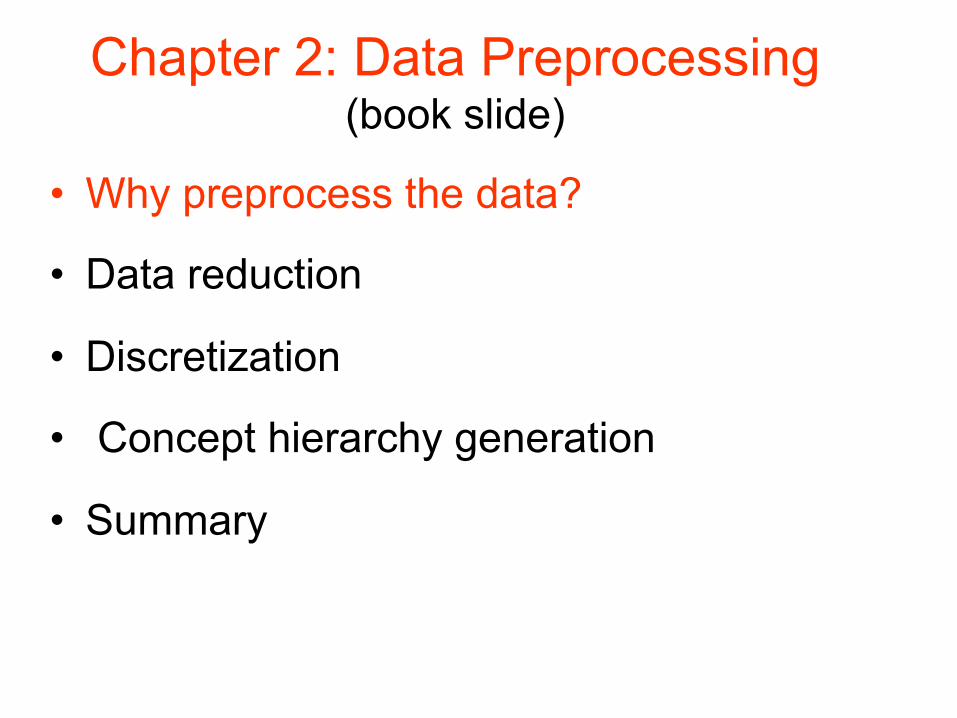
Why Data Preprocessing? (book slide)
• Data in the real world is dirty – incomplete: lacking attribute values, lacking
certain attributes of interest, or containing only aggregate data
• e.g., occupation=“ ” – noisy: containing errors or outliers
• e.g., Salary=“-10” – inconsistent: containing discrepancies in
codes or names • e.g., Age=“42” Birthday=“03/07/1997” • e.g., Was rating “1,2,3”, now rating “A, B, C” • e.g., discrepancy between duplicate records
Why Is Data Dirty? (book slide)
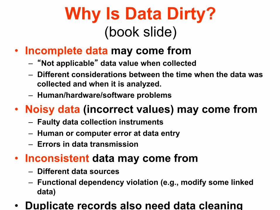
• Incomplete data may come from – “Not applicable” data value when collected – Different considerations between the time when the data was
collected and when it is analyzed. – Human/hardware/software problems
• Noisy data (incorrect values) may come from – Faulty data collection instruments – Human or computer error at data entry – Errors in data transmission
• Inconsistent data may come from – Different data sources – Functional dependency violation (e.g., modify some linked
data)
• Duplicate records also need data cleaning
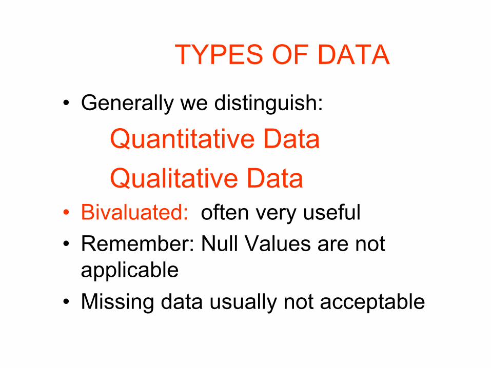
TYPES OF DATA
• Generally we distinguish:
Quantitative Data Qualitative Data
• Bivaluated: often very useful • Remember: Null Values are not
applicable • Missing data usually not acceptable
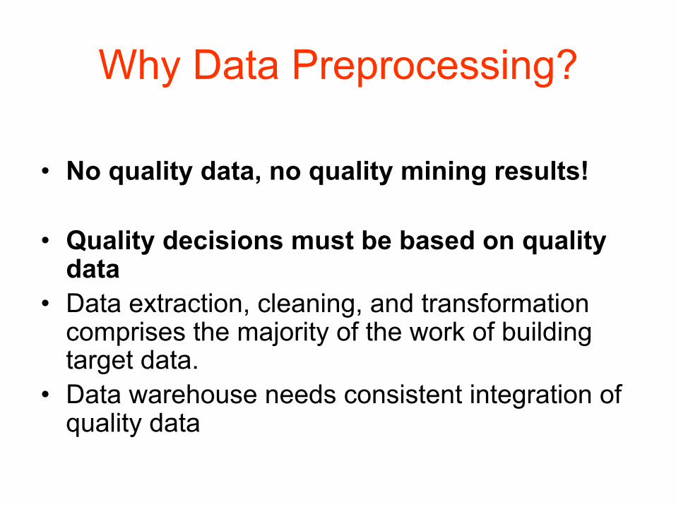
Why Data Preprocessing?
• No quality data, no quality mining results!
• Quality decisions must be based on quality data
• Data extraction, cleaning, and transformation comprises the majority of the work of building target data.
• Data warehouse needs consistent integration of quality data

Measures of Data Quality
• A well-accepted multidimensional view of data quality: – Accuracy – Completeness – Consistency – Timeliness – Believability – Interpretability – Accessibility
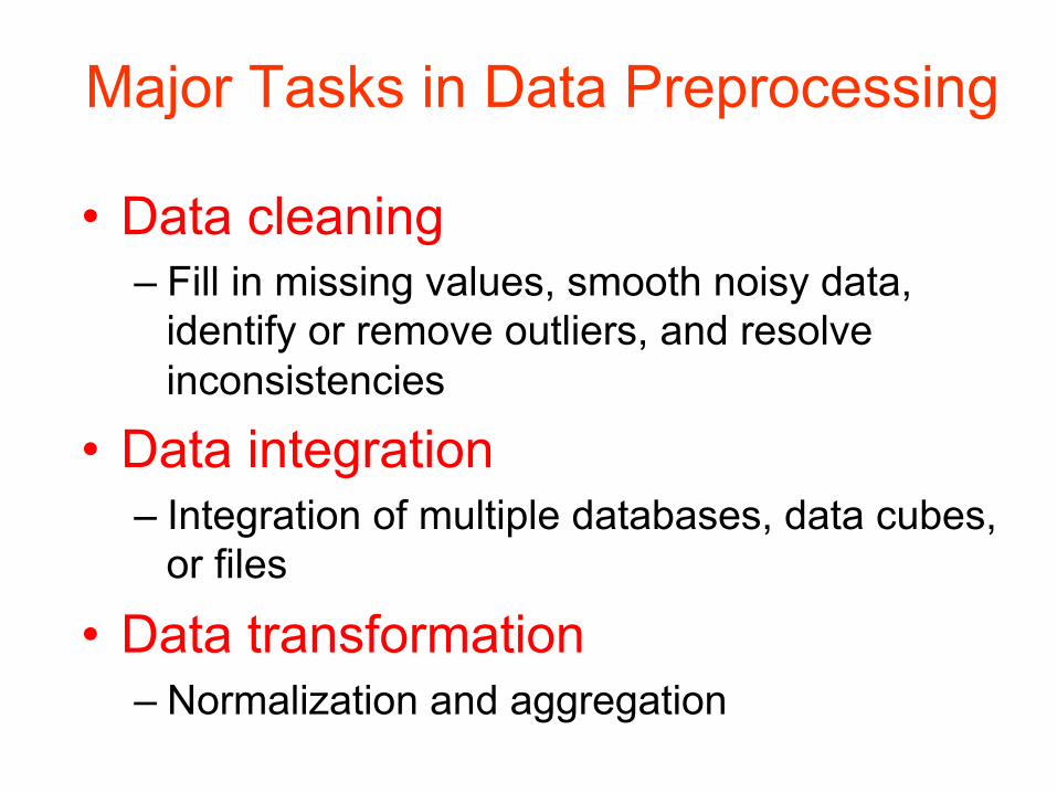
Major Tasks in Data Preprocessing
• Data cleaning – Fill in missing values, smooth noisy data,
identify or remove outliers, and resolve inconsistencies
• Data integration – Integration of multiple databases, data cubes,
or files
• Data transformation – Normalization and aggregation
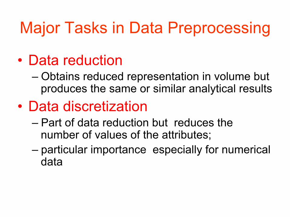
Major Tasks in Data Preprocessing
• Data reduction – Obtains reduced representation in volume but
produces the same or similar analytical results
• Data discretization – Part of data reduction but reduces the
number of values of the attributes; – particular importance especially for numerical
data
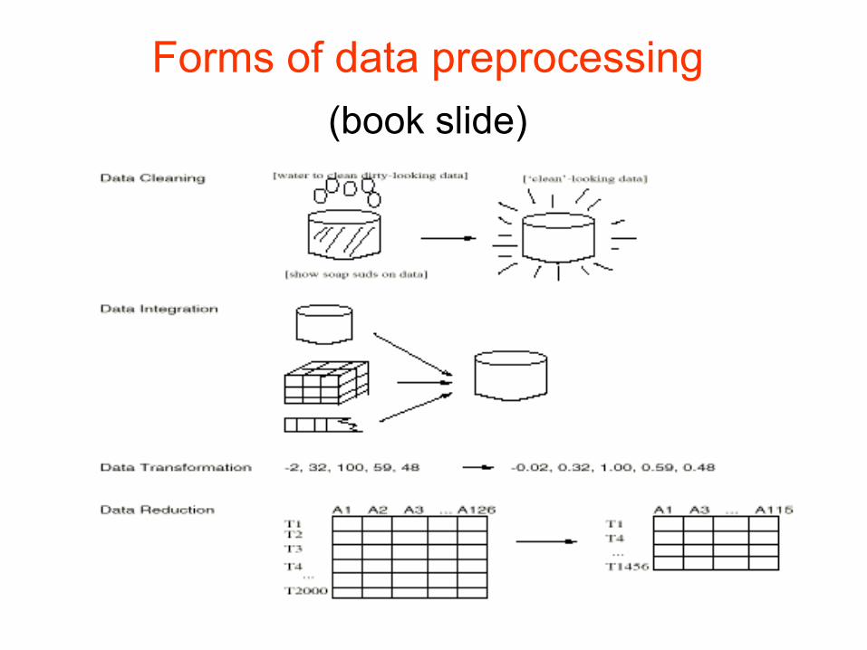
Forms of data preprocessing (book slide)
Descriptive Data Summarization
– Descriptive Data Summarization techniques are used to identify the typical properties of the data and highlight which data values should be treated as nose or outliers
– WE WANT TO LEARN ABOUT THE DATA CHARACTERISTCS REGARDING BOTH : CENTRALTENDENCY AND DISPERSION OF THE DATA.

Descriptive Data Summarization – Measures of CENTRALTENDENCY are:
mean, median, mode, and midrange.
– Dispersion, or variance of the data is the degree to which numerical data tend to spread.
– Data Dispersion Measures: – Range, the five-number summary (based
on quartiles), the interquartile range, and standard deviation.

Measuring the Central Tendency (for values xi of an attribute)
• MEAN is a distributive measure, i.e. it can be computed on subsets , and results merged in one MEAN:
• n is the number of records in the set (subset)
• MEAN is also an algebraic measure , i.e. it is a measure that can be computed by applying an algebraic function to one or more distributive measures.
∑=
=n
iixn
x1
1
Nx∑=µ
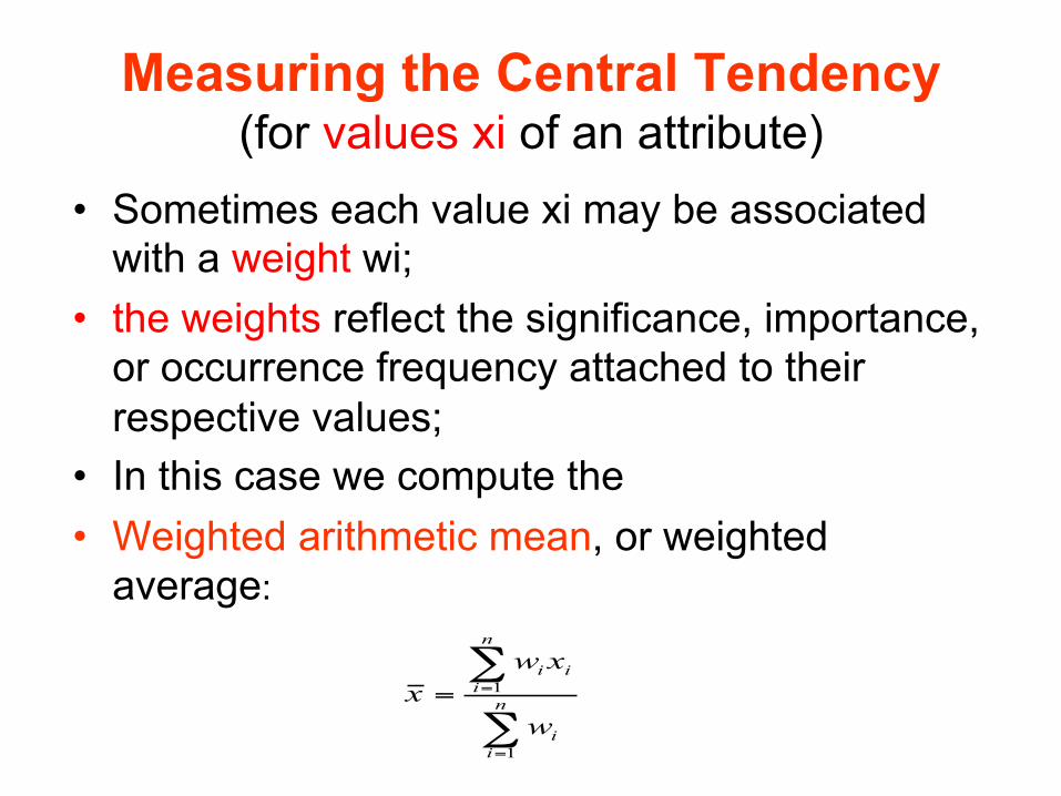
Measuring the Central Tendency (for values xi of an attribute)
• Sometimes each value xi may be associated with a weight wi;
• the weights reflect the significance, importance, or occurrence frequency attached to their respective values;
• In this case we compute the • Weighted arithmetic mean, or weighted
average:
∑
∑
=
== n
ii
n
iii
w
xwx
1
1
Measuring the Central Tendency (for values of an attribute)
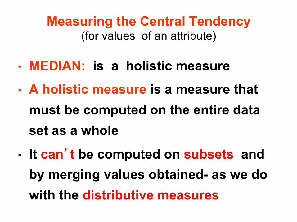
• MEDIAN: is a holistic measure
• A holistic measure is a measure that must be computed on the entire data set as a whole
• It can’t be computed on subsets and by merging values obtained- as we do with the distributive measures
Measuring the Central Tendency (for values of an attribute)
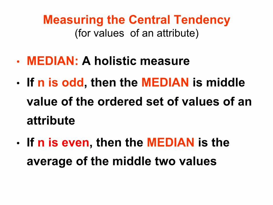
• MEDIAN: A holistic measure
• If n is odd, then the MEDIAN is middle value of the ordered set of values of an attribute
• If n is even, then the MEDIAN is the average of the middle two values
Measuring the Central Tendency (for values of an attribute)
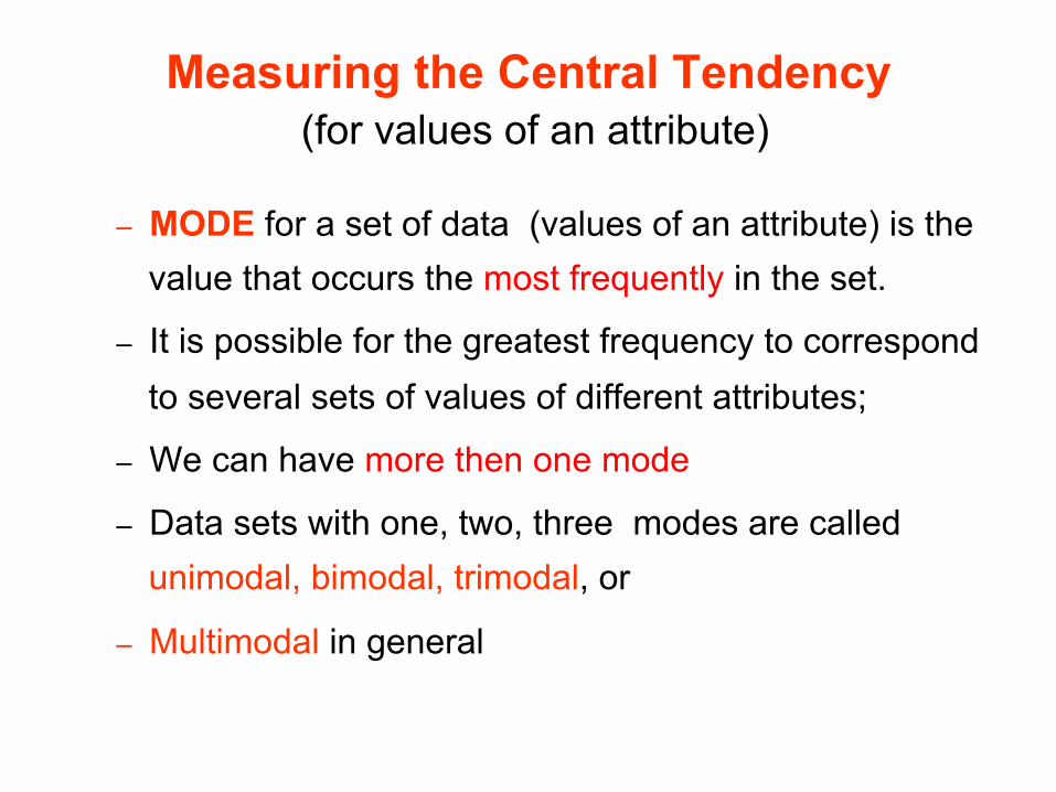
– MODE for a set of data (values of an attribute) is the value that occurs the most frequently in the set.
– It is possible for the greatest frequency to correspond to several sets of values of different attributes;
– We can have more then one mode
– Data sets with one, two, three modes are called unimodal, bimodal, trimodal, or
– Multimodal in general
Measuring the Dispersion of Data (book slide)
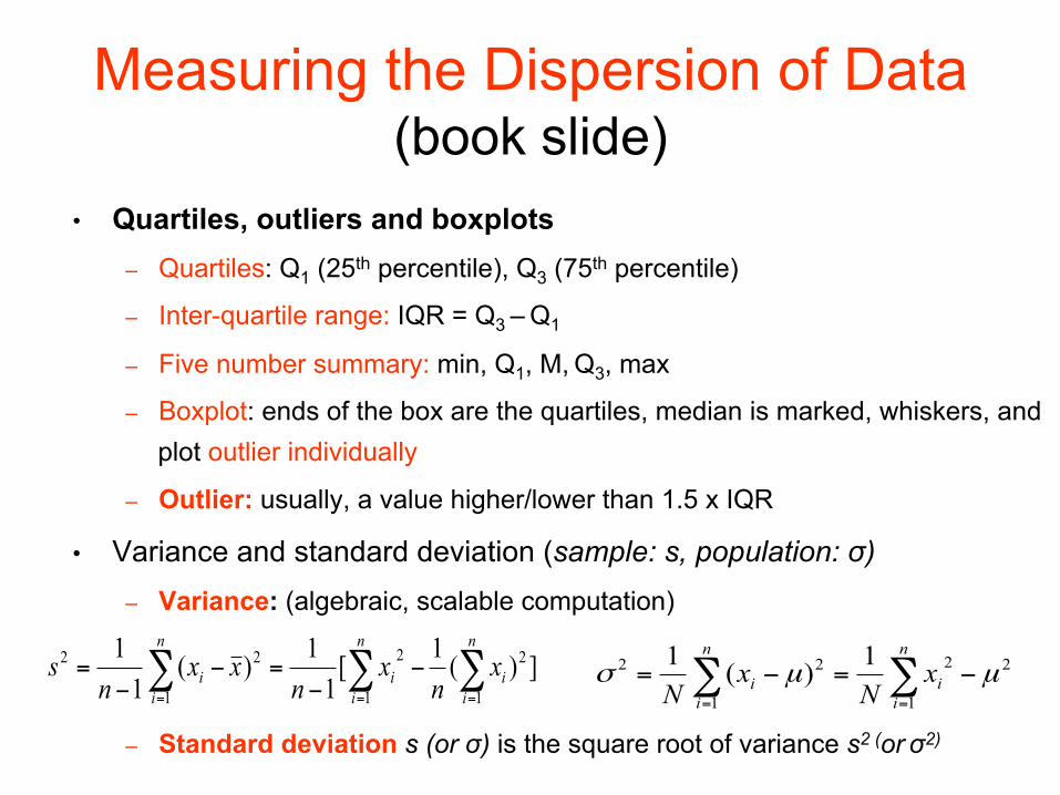
• Quartiles, outliers and boxplots – Quartiles: Q1 (25th percentile), Q3 (75th percentile)
– Inter-quartile range: IQR = Q3 – Q1
– Five number summary: min, Q1, M, Q3, max
– Boxplot: ends of the box are the quartiles, median is marked, whiskers, and plot outlier individually
– Outlier: usually, a value higher/lower than 1.5 x IQR
• Variance and standard deviation (sample: s, population: σ) – Variance: (algebraic, scalable computation)
– Standard deviation s (or σ) is the square root of variance s2 (or σ2)
∑ ∑∑= ==
−−
=−−
=n
i
n
iii
n
ii x
nx
nxx
ns
1 1
22
1
22 ])(1[11)(
11
∑∑==
−=−=n
ii
n
ii x
Nx
N 1
22
1
22 1)(1µµσ
Data Cleaning
• Data cleaning tasks:
– Fill in missing values
– Identify outliers and smooth out noisy data
– Correct inconsistent data
– Resolve redundancy caused by data integration
Missing Data • Some Data is not always available
– E.g., many tuples have no recorded value for several attributes, such as customer income in sales data
• Missing data may be due to – equipment malfunction – inconsistent with other recorded data and thus deleted
– data not entered due to misunderstanding
– certain data may not be considered important at the time of entry
– not register history or changes of the data
• Missing data may need to be inferred
How to Handle Missing Data?
• (1) Ignore the tuple (record) : usually done
when class label is missing (assuming the tasks
in classification)
• It is not effective when the percentage of missing values per attribute varies considerably.
• (2) Fill in the missing value manually: tedious +
infeasible?
How to Handle Missing Data? • (3) Use a global constant to fill in the missing value (be
careful- it introduces a new class)
• (4) Use the attribute values mean to fill in the missing
value
• (5) Use the attribute values mean for all samples
belonging to the same class to fill in the missing value:
smarter then (4) in case of classification
• (6) Use the most probable value to fill in the missing
value
• (7) Use regresion methods
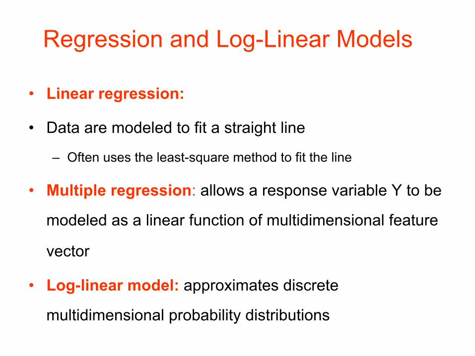
Regression and Log-Linear Models
• Linear regression:
• Data are modeled to fit a straight line
– Often uses the least-square method to fit the line
• Multiple regression: allows a response variable Y to be
modeled as a linear function of multidimensional feature
vector
• Log-linear model: approximates discrete
multidimensional probability distributions
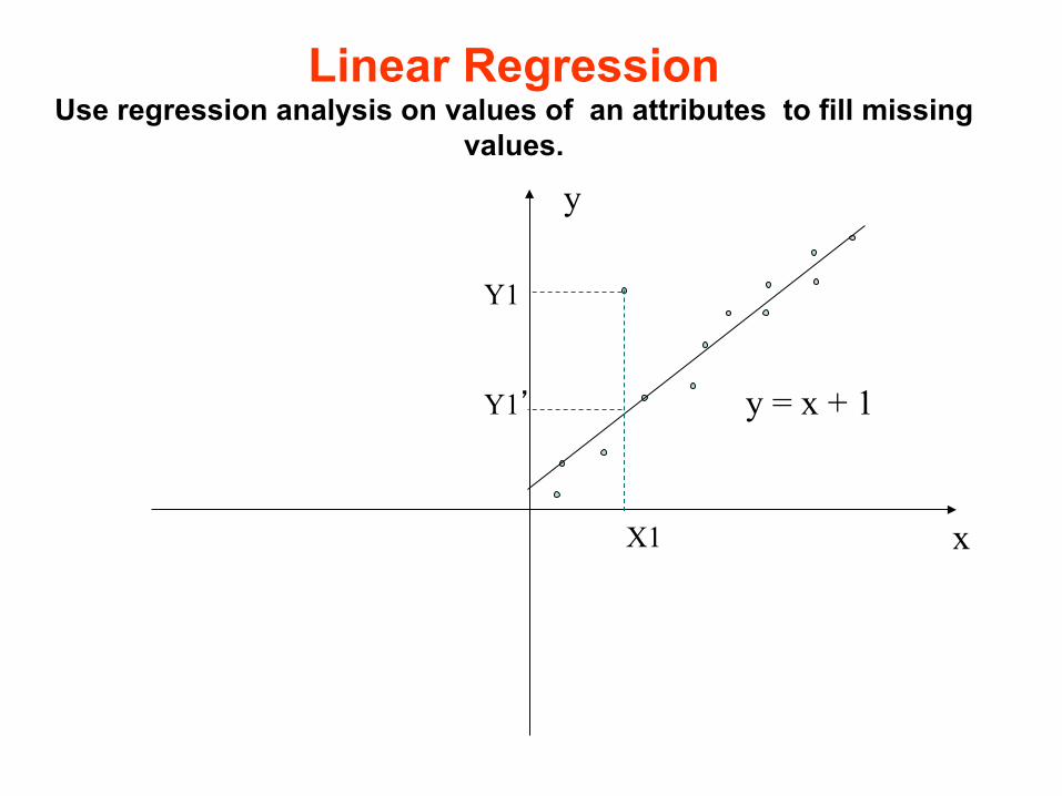
Linear Regression Use regression analysis on values of an attributes to fill missing
values.
x
y
y = x + 1
X1
Y1
Y1’
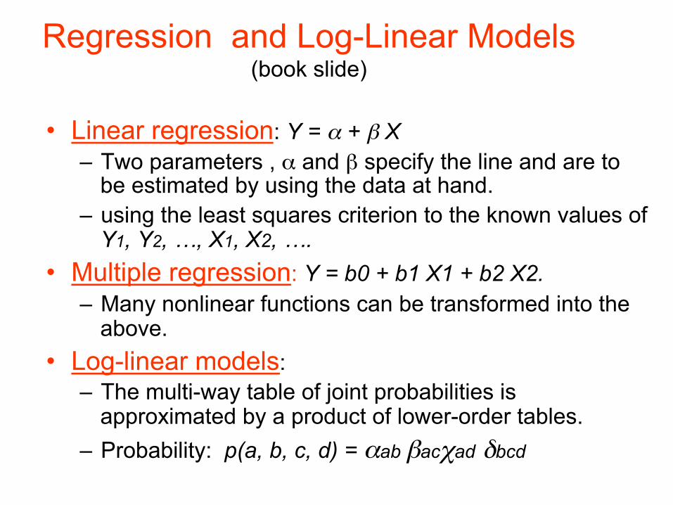
• Linear regression: Y = α + β X – Two parameters , α and β specify the line and are to
be estimated by using the data at hand. – using the least squares criterion to the known values of
Y1, Y2, …, X1, X2, …. • Multiple regression: Y = b0 + b1 X1 + b2 X2.
– Many nonlinear functions can be transformed into the above.
• Log-linear models: – The multi-way table of joint probabilities is
approximated by a product of lower-order tables. – Probability: p(a, b, c, d) = αab βacχad δbcd
Regression and Log-Linear Models (book slide)
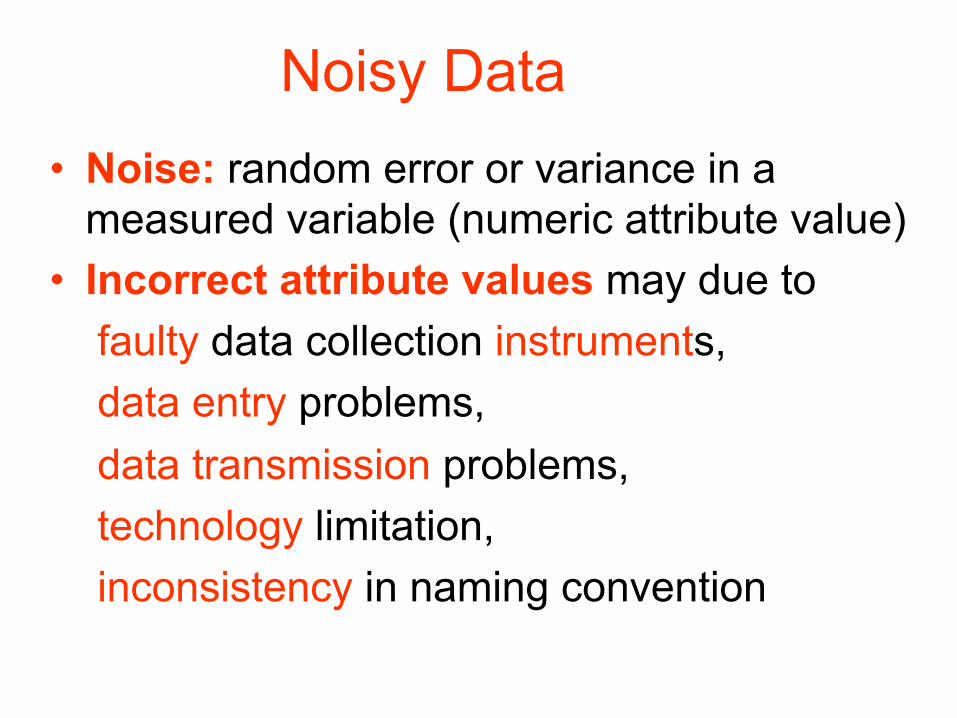
Noisy Data • Noise: random error or variance in a
measured variable (numeric attribute value) • Incorrect attribute values may due to
faulty data collection instruments, data entry problems, data transmission problems, technology limitation, inconsistency in naming convention

Other Data Problems
• Other data problems which requires data cleaning – duplicate records – incomplete data – inconsistent data

How to Handle Noisy Data?
• Clustering – detect and remove outliers
• Combined computer and human inspection – detect suspicious values and check by human
• Regression – smooth by fitting the data into regression
functions
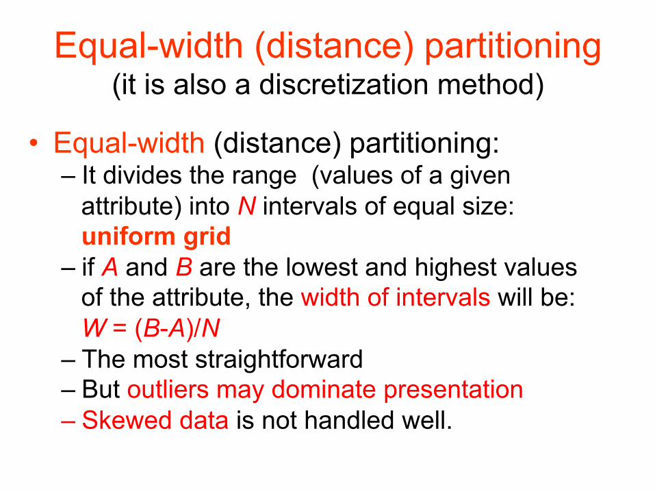
Equal-width (distance) partitioning (it is also a discretization method)
• Equal-width (distance) partitioning: – It divides the range (values of a given
attribute) into N intervals of equal size: uniform grid
– if A and B are the lowest and highest values of the attribute, the width of intervals will be: W = (B-A)/N
– The most straightforward – But outliers may dominate presentation – Skewed data is not handled well.
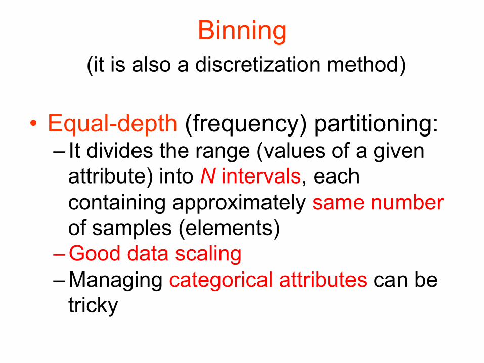
Binning (it is also a discretization method)
• Equal-depth (frequency) partitioning: – It divides the range (values of a given
attribute) into N intervals, each containing approximately same number of samples (elements)
– Good data scaling – Managing categorical attributes can be
tricky
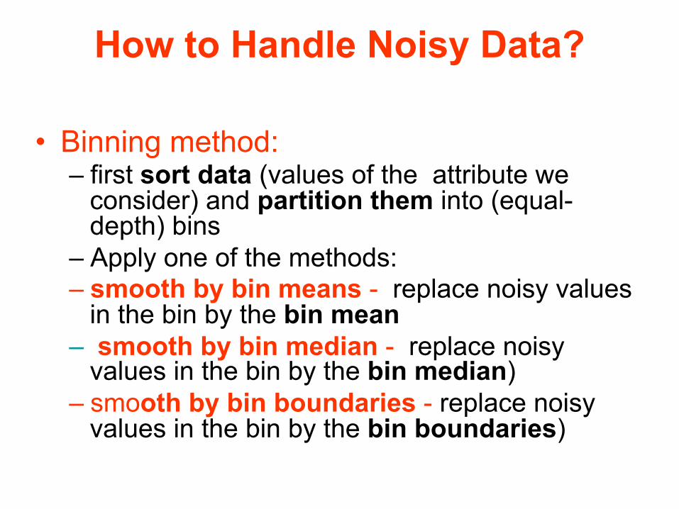
How to Handle Noisy Data?
• Binning method: – first sort data (values of the attribute we
consider) and partition them into (equal-depth) bins
– Apply one of the methods: – smooth by bin means - replace noisy values
in the bin by the bin mean – smooth by bin median - replace noisy
values in the bin by the bin median) – smooth by bin boundaries - replace noisy
values in the bin by the bin boundaries)
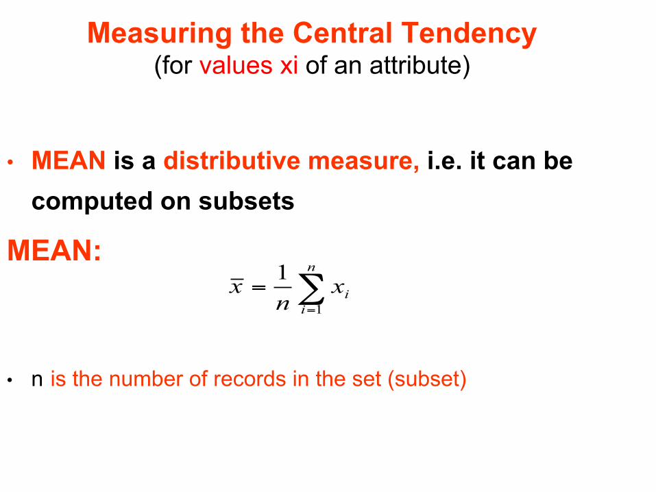
Measuring the Central Tendency (for values xi of an attribute)
• MEAN is a distributive measure, i.e. it can be computed on subsets
MEAN:
• n is the number of records in the set (subset)
∑=
=n
iixn
x1
1
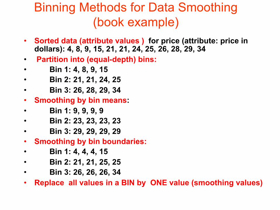
Binning Methods for Data Smoothing (book example)
• Sorted data (attribute values ) for price (attribute: price in dollars): 4, 8, 9, 15, 21, 21, 24, 25, 26, 28, 29, 34
• Partition into (equal-depth) bins: • Bin 1: 4, 8, 9, 15 • Bin 2: 21, 21, 24, 25 • Bin 3: 26, 28, 29, 34 • Smoothing by bin means: • Bin 1: 9, 9, 9, 9 • Bin 2: 23, 23, 23, 23 • Bin 3: 29, 29, 29, 29 • Smoothing by bin boundaries: • Bin 1: 4, 4, 4, 15 • Bin 2: 21, 21, 25, 25 • Bin 3: 26, 26, 26, 34 • Replace all values in a BIN by ONE value (smoothing values)

Data Integration • Data integration:
– combines data from multiple sources into a coherent store
• Schema integration – integrate metadata from different sources – Entity identification problem: identify real world entities
from multiple data sources, e.g., A.cust-id ≡ B.cust-# • Detecting and resolving data value conflicts
– for the same real world entity, attribute values from different sources are different
– possible reasons: different representations, different scales, e.g., metric vs. British units
Handling Redundancy in Data Integration
• Redundant data occur often when integration of multiple databases – Object identification: The same attribute or object
may have different names in different databases – Derivable data: One attribute may be a “derived”
attribute in another table, e.g., annual revenue
• Redundant attributes may be able to be detected by correlation analysis
• Careful integration of the data from multiple sources may help reduce/avoid redundancies and inconsistencies and improve mining speed and quality
Data Cleaning as a Process (book slide)
• Data discrepancy detection – Use metadata (e.g., domain, range, dependency, distribution) – Check field overloading – Check uniqueness rule, consecutive rule and null rule – Use commercial tools
• Data scrubbing: use simple domain knowledge (e.g., postal code, spell-check) to detect errors and make corrections
• Data auditing: by analyzing data to discover rules and relationship to detect violators (e.g., correlation and clustering to find outliers)
• Data migration and integration – Data migration tools: allow transformations to be specified – ETL (Extraction/Transformation/Loading) tools: allow users to
specify transformations through a graphical user interface • Integration of the two processes
– Iterative and interactive (e.g., Potter’s Wheels)
Chapter 2: Data Preprocessing (book slide)
• Why preprocess the data?
• Data cleaning
• Data integration and transformation
• Data reduction
• Discretization and concept hierarchy
generation
• Summary
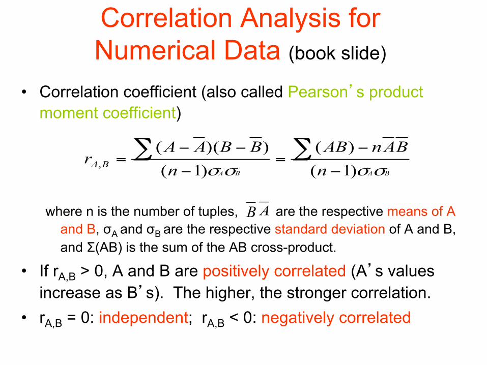
Correlation Analysis for Numerical Data (book slide)
• Correlation coefficient (also called Pearson’s product moment coefficient)
where n is the number of tuples, are the respective means of A and B, σA and σB are the respective standard deviation of A and B, and Σ(AB) is the sum of the AB cross-product.
• If rA,B > 0, A and B are positively correlated (A’s values increase as B’s). The higher, the stronger correlation.
• rA,B = 0: independent; rA,B < 0: negatively correlated
BABA nBAnAB
nBBAA
r BA σσσσ )1()(
)1())((
, −
−=
−
−−= ∑∑
AB
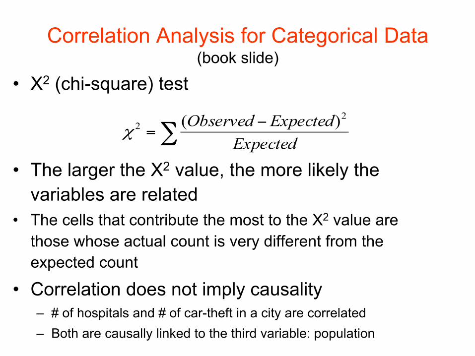
Correlation Analysis for Categorical Data (book slide)
• Χ2 (chi-square) test
• The larger the Χ2 value, the more likely the variables are related
• The cells that contribute the most to the Χ2 value are those whose actual count is very different from the expected count
• Correlation does not imply causality – # of hospitals and # of car-theft in a city are correlated – Both are causally linked to the third variable: population
∑−
=Expected
ExpectedObserved 22 )(
χ
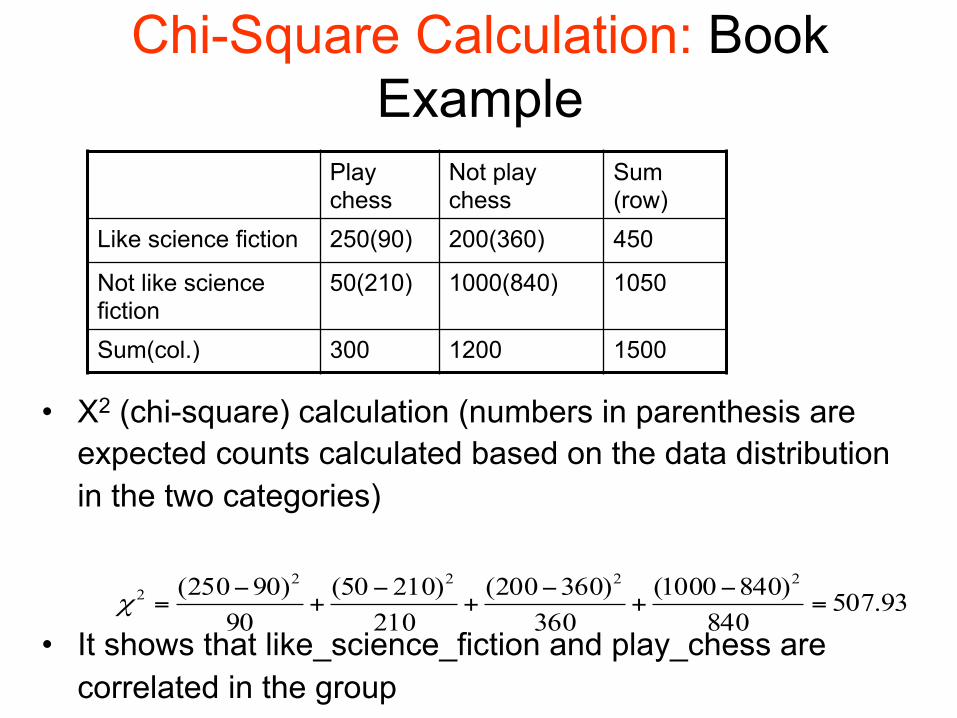
Chi-Square Calculation: Book Example
• Χ2 (chi-square) calculation (numbers in parenthesis are expected counts calculated based on the data distribution in the two categories)
• It shows that like_science_fiction and play_chess are correlated in the group
93.507840
)8401000(360
)360200(210
)21050(90
)90250( 22222 =
−+
−+
−+
−=χ
Play chess
Not play chess
Sum (row)
Like science fiction 250(90) 200(360) 450
Not like science fiction
50(210) 1000(840) 1050
Sum(col.) 300 1200 1500

Data Transformation (book slide)
• Smoothing: remove noise from data • Aggregation: summarization, data cube construction • Generalization: • concept hierarchy Normalization: scaled to fall within a small,
specified range – min-max normalization – z-score normalization – normalization by decimal scaling
• Attribute/feature construction – New attributes constructed from the given ones
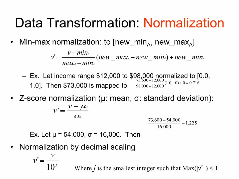
Data Transformation: Normalization • Min-max normalization: to [new_minA, new_maxA]
– Ex. Let income range $12,000 to $98,000 normalized to [0.0, 1.0]. Then $73,000 is mapped to
• Z-score normalization (µ: mean, σ: standard deviation):
– Ex. Let µ = 54,000, σ = 16,000. Then
• Normalization by decimal scaling
716.00)00.1(000,12000,98000,12600,73
=+−−
−
AAA
AA
A minnewminnewmaxnewminmaxminvv _)__(' +−−
−=
A
Avvσµ−
='
j
vv10
'=Where j is the smallest integer such that Max(|ν’|) < 1
225.1000,16
000,54600,73=
−
Chapter 2: Data Preprocessing (book slide)
• Why preprocess the data?
• Data cleaning
• Data integration and transformation
• Data reduction
• Discretization and concept hierarchy
generation
• Summary
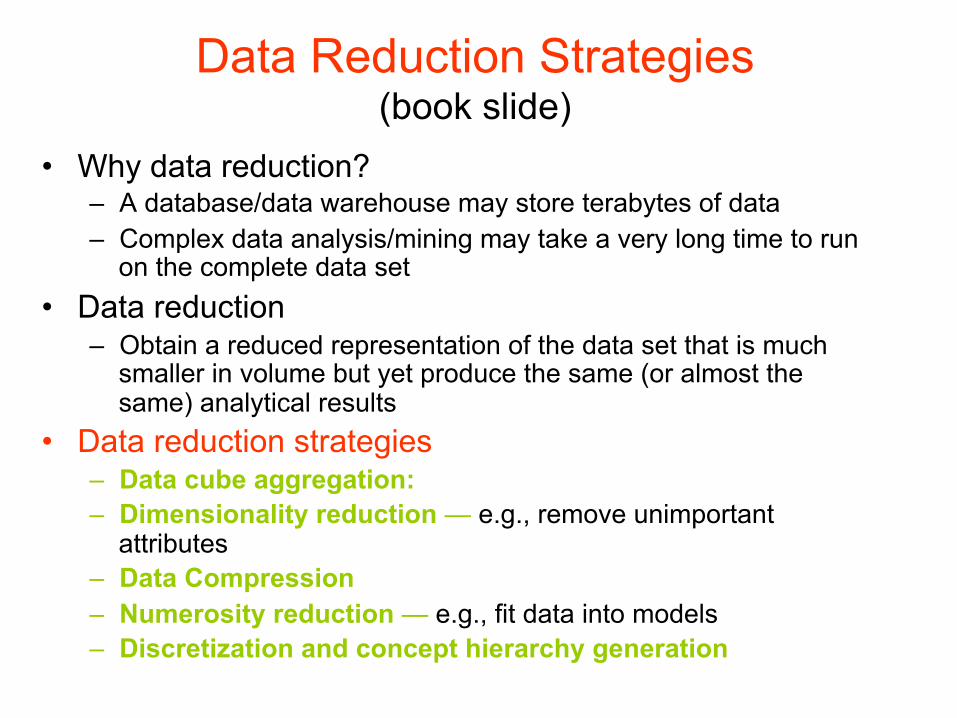
Data Reduction Strategies (book slide)
• Why data reduction? – A database/data warehouse may store terabytes of data – Complex data analysis/mining may take a very long time to run
on the complete data set • Data reduction
– Obtain a reduced representation of the data set that is much smaller in volume but yet produce the same (or almost the same) analytical results
• Data reduction strategies – Data cube aggregation: – Dimensionality reduction — e.g., remove unimportant
attributes – Data Compression – Numerosity reduction — e.g., fit data into models – Discretization and concept hierarchy generation
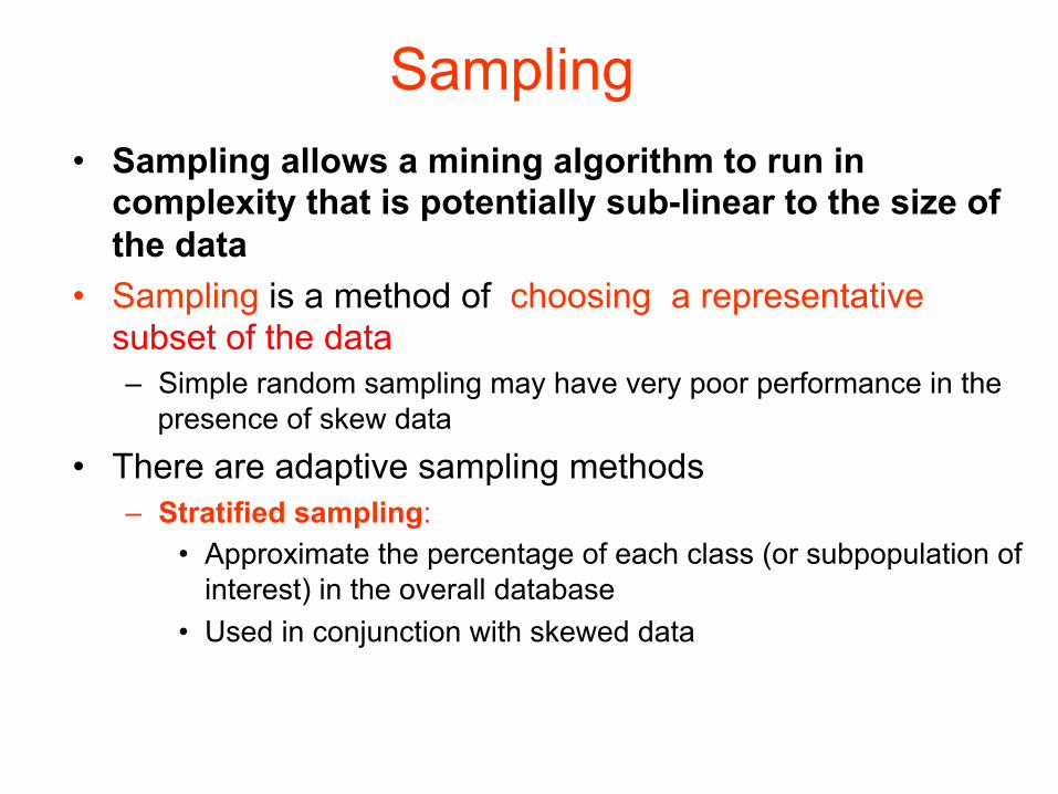
Sampling • Sampling allows a mining algorithm to run in
complexity that is potentially sub-linear to the size of the data
• Sampling is a method of choosing a representative subset of the data – Simple random sampling may have very poor performance in the
presence of skew data
• There are adaptive sampling methods – Stratified sampling:
• Approximate the percentage of each class (or subpopulation of interest) in the overall database
• Used in conjunction with skewed data
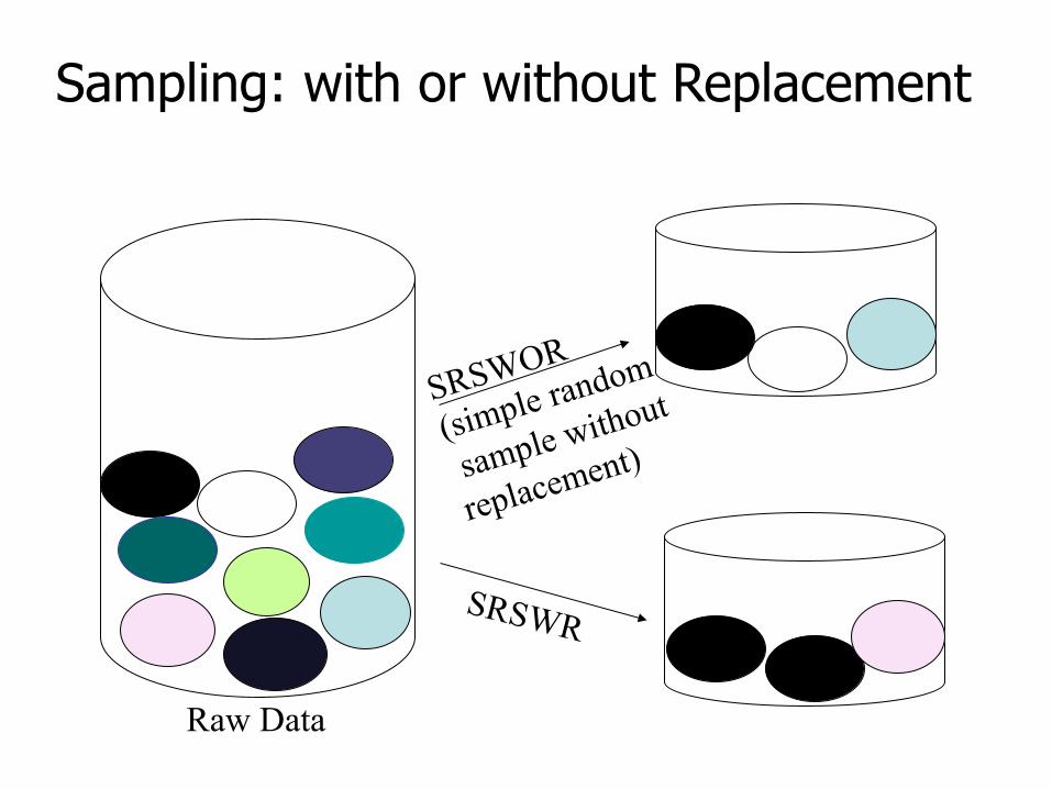
Sampling: with or without Replacement
SRSWOR
(simple random
sample without
replacement)
SRSWR
Raw Data
Attribute Subset Selection
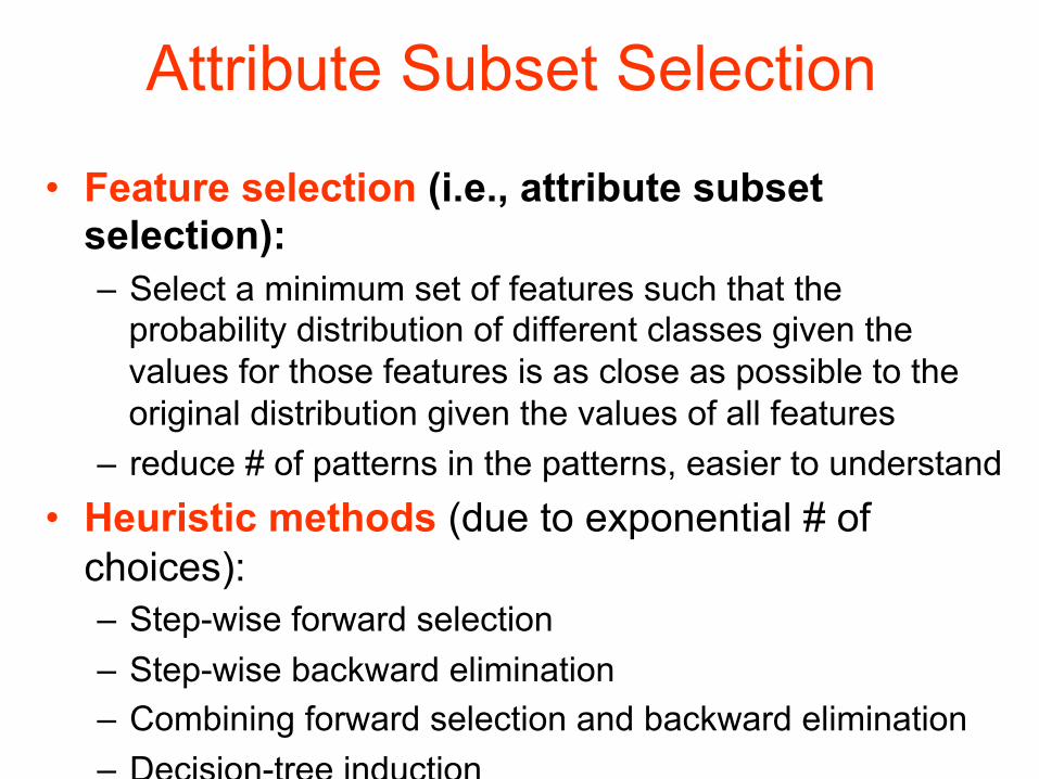
• Feature selection (i.e., attribute subset selection): – Select a minimum set of features such that the
probability distribution of different classes given the values for those features is as close as possible to the original distribution given the values of all features
– reduce # of patterns in the patterns, easier to understand • Heuristic methods (due to exponential # of
choices): – Step-wise forward selection – Step-wise backward elimination – Combining forward selection and backward elimination – Decision-tree induction
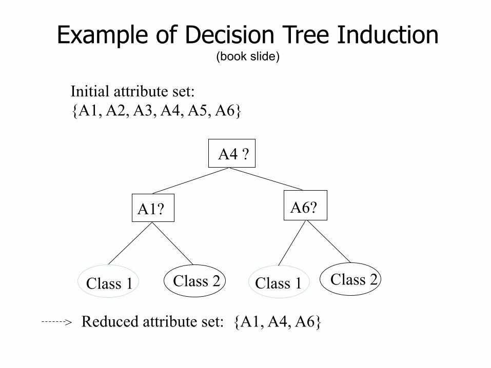
Example of Decision Tree Induction (book slide)
Initial attribute set: {A1, A2, A3, A4, A5, A6}
A4 ?
A1? A6?
Class 1 Class 2 Class 1 Class 2
> Reduced attribute set: {A1, A4, A6}
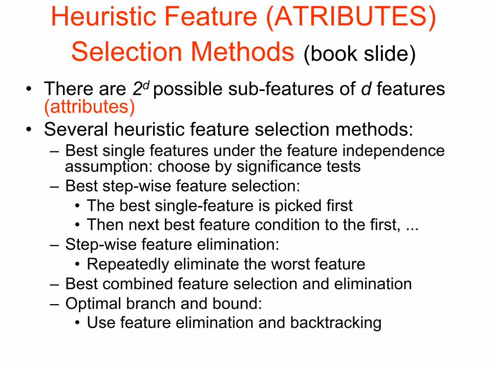
Heuristic Feature (ATRIBUTES) Selection Methods (book slide)
• There are 2d possible sub-features of d features (attributes)
• Several heuristic feature selection methods: – Best single features under the feature independence
assumption: choose by significance tests – Best step-wise feature selection:
• The best single-feature is picked first • Then next best feature condition to the first, ...
– Step-wise feature elimination: • Repeatedly eliminate the worst feature
– Best combined feature selection and elimination – Optimal branch and bound:
• Use feature elimination and backtracking
Data Compression (book slide)
• String compression – There are extensive theories and well-tuned algorithms – Typically lossless – But only limited manipulation is possible without
expansion • Audio/video compression
– Typically lossy compression, with progressive refinement
– Sometimes small fragments of signal can be reconstructed without reconstructing the whole
• Time sequence is not audio – Typically short and vary slowly with time
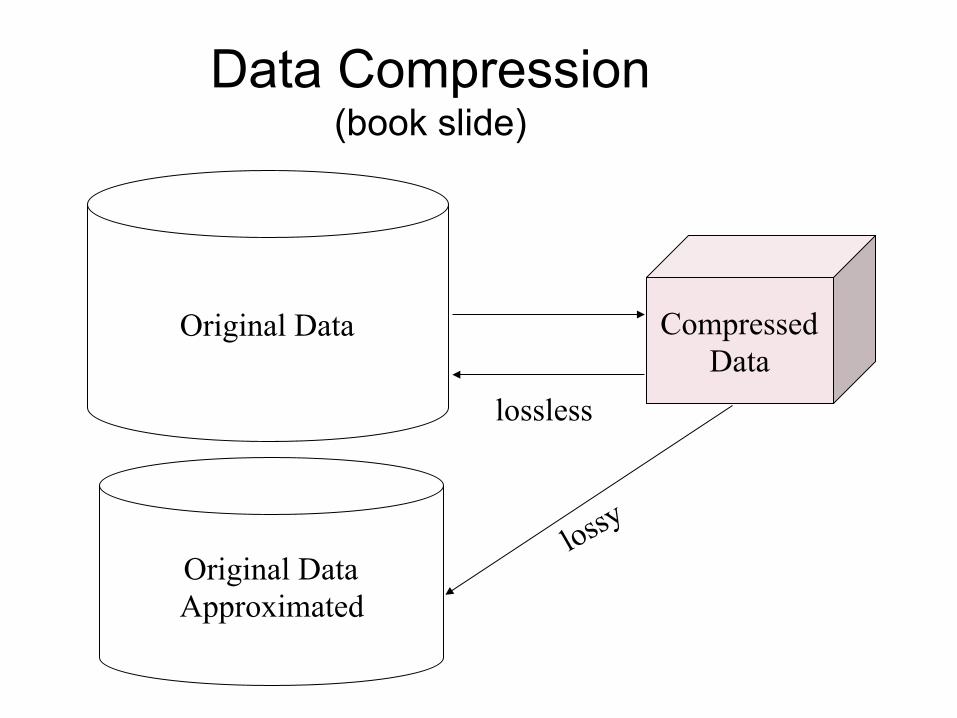
Data Compression (book slide)
Original Data Compressed Data
lossless
Original Data Approximated
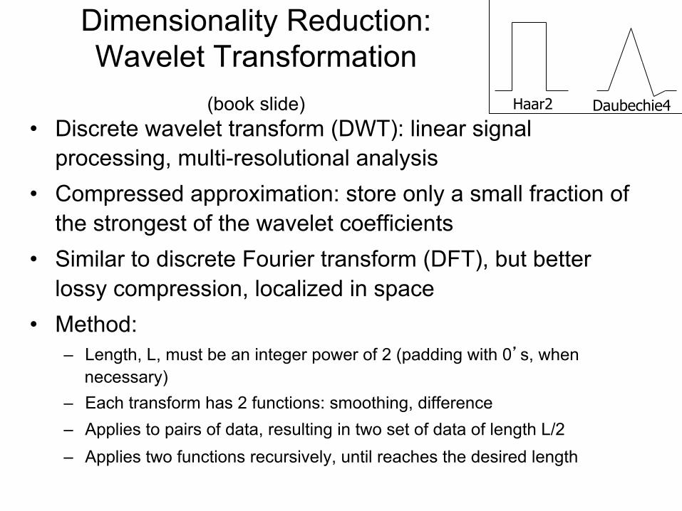
Dimensionality Reduction: Wavelet Transformation
(book slide) • Discrete wavelet transform (DWT): linear signal
processing, multi-resolutional analysis • Compressed approximation: store only a small fraction of
the strongest of the wavelet coefficients • Similar to discrete Fourier transform (DFT), but better
lossy compression, localized in space • Method:
– Length, L, must be an integer power of 2 (padding with 0’s, when necessary)
– Each transform has 2 functions: smoothing, difference – Applies to pairs of data, resulting in two set of data of length L/2 – Applies two functions recursively, until reaches the desired length
Haar2 Daubechie4
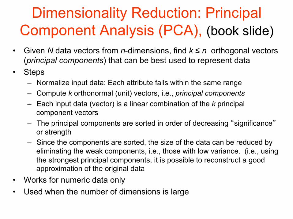
• Given N data vectors from n-dimensions, find k ≤ n orthogonal vectors (principal components) that can be best used to represent data
• Steps – Normalize input data: Each attribute falls within the same range – Compute k orthonormal (unit) vectors, i.e., principal components – Each input data (vector) is a linear combination of the k principal
component vectors – The principal components are sorted in order of decreasing “significance”
or strength – Since the components are sorted, the size of the data can be reduced by
eliminating the weak components, i.e., those with low variance. (i.e., using the strongest principal components, it is possible to reconstruct a good approximation of the original data
• Works for numeric data only • Used when the number of dimensions is large
Dimensionality Reduction: Principal Component Analysis (PCA), (book slide)
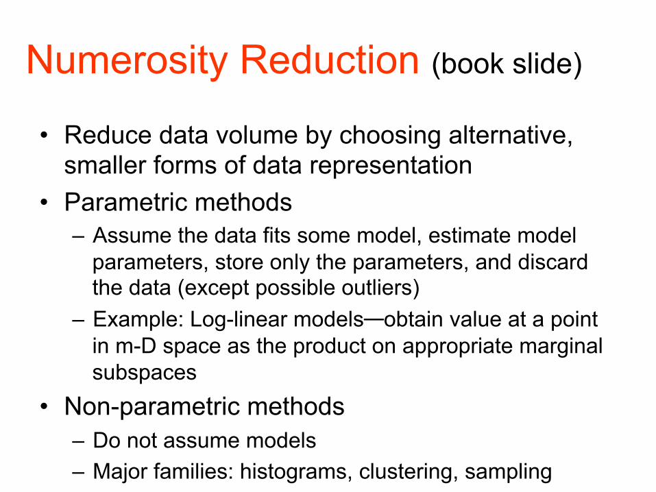
Numerosity Reduction (book slide)
• Reduce data volume by choosing alternative, smaller forms of data representation
• Parametric methods – Assume the data fits some model, estimate model
parameters, store only the parameters, and discard the data (except possible outliers)
– Example: Log-linear models—obtain value at a point in m-D space as the product on appropriate marginal subspaces
• Non-parametric methods – Do not assume models – Major families: histograms, clustering, sampling
Data Reduction Method (1): Regression and Log-Linear Models (book slide)
• Linear regression: Data are modeled to fit a
straight line
– Often uses the least-square method to fit the line
• Multiple regression: allows a response variable
Y to be modeled as a linear function of
multidimensional feature vector
• Log-linear model: approximates discrete
multidimensional probability distributions

• Linear regression: Y = w X + b – Two regression coefficients, w and b, specify the line
and are to be estimated by using the data at hand – Using the least squares criterion to the known values
of Y1, Y2, …, X1, X2, …. • Multiple regression: Y = b0 + b1 X1 + b2 X2.
– Many nonlinear functions can be transformed into the above
• Log-linear models: – The multi-way table of joint probabilities is
approximated by a product of lower-order tables – Probability: p(a, b, c, d) = αab βacχad δbcd
Regress Analysis and Log-Linear Models

Data Reduction Method (2): Histograms (book slide)
Divide data (values of an attribute) into buckets and store average (sum) for each bucket
Partitioning rules: Equal-width: equal bucket range Equal-frequency (or equal-depth)
V-optimal: with the least histogram variance (weighted sum of the original values that each bucket represents)
MaxDiff: set bucket boundary between each pair for pairs have the β–1 largest differences
0
5
10
15
20
25
30
35
40
10000 20000 30000 40000 50000 60000 70000 80000 90000 100000
Data Reduction Method (3): Clustering
• Partition data set into clusters based on similarity, and store cluster representation (e.g., centroid and diameter) only
• Can be very effective if data is clustered but not if data is “smeared”
• Can have hierarchical clustering and be stored in multi-dimensional index tree structures
• There are many choices of clustering definitions and clustering algorithms
• Cluster analysis will be studied in depth in Chapter 7
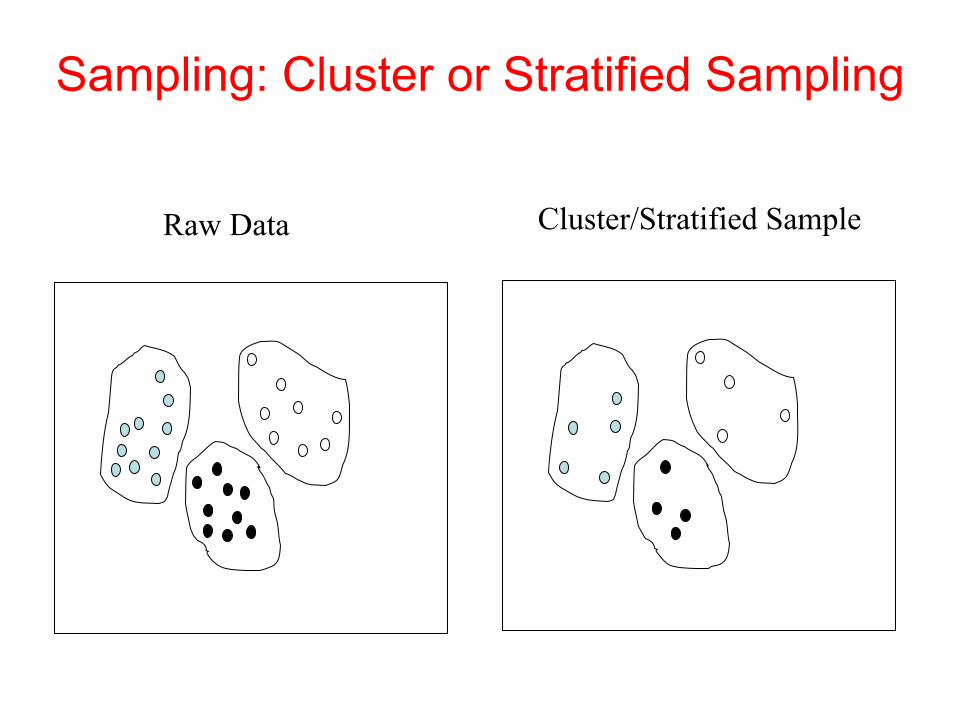
Sampling: Cluster or Stratified Sampling
Raw Data Cluster/Stratified Sample

Chapter 2: Data Preprocessing (book slide)
• Why preprocess the data?
• Data cleaning
• Data integration and transformation
• Data reduction
• Discretization and concept hierarchy
generation
• Summary
Discretization • Three types of attributes:
– Nominal — values from an unordered set – Ordinal — values from an ordered set – Continuous — real numbers
• Discretization: • divide the range of a continuous attribute into
intervals – Some classification algorithms only accept
categorical (non- numerical) attributes. – Reduce data (attributes values) size by discretization – Prepare for further analysis
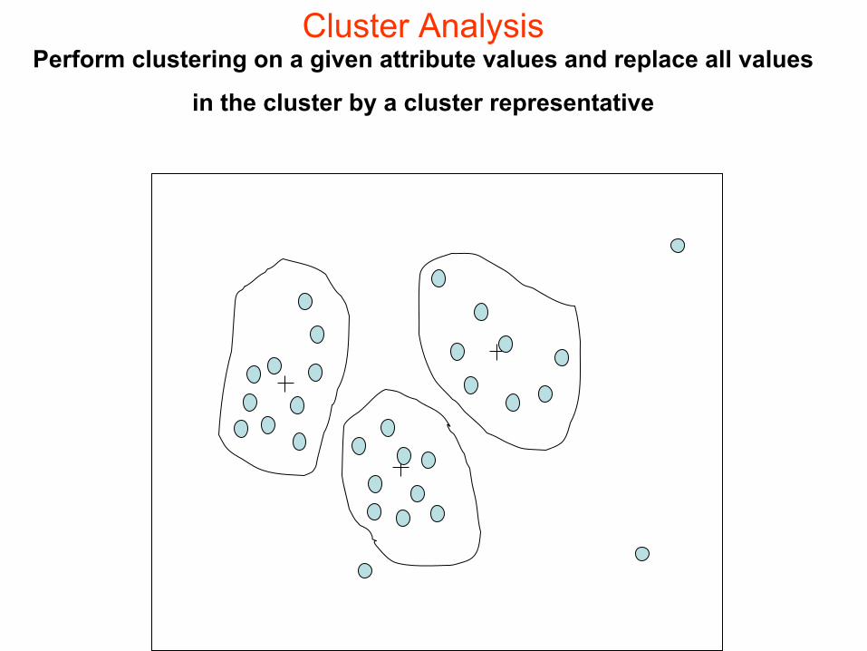
Cluster Analysis Perform clustering on a given attribute values and replace all values
in the cluster by a cluster representative
Discretization and Concept Hierachy
• Discretization – reduce the number of values for a given continuous
attribute by dividing the range of the attribute (values of the attribute) into intervals. Interval labels are then used to replace actual data values.
• Concept hierarchies – reduce the data by collecting and replacing low level
concepts (such as numeric values for the attribute age) by higher level concepts (such as young, middle-aged, or senior).
Discretization and concept hierarchy generation for numeric data
• Discretization:
• Binning (see sections before)
• Histogram analysis (see sections before)
• Clustering analysis (see sections before)
• Entropy-based discretization
• Segmentation by natural partitioning

Entropy-Based Discretization book slide
• Given a set of samples S (here numerical values on an attribute), if S is partitioned into two intervals S1 and S2 using boundary T, the entropy after partitioning is
• The boundary that minimizes the entropy function over all possible boundaries is selected as a binary discretization.
• The process is recursively applied to partitions obtained until some stopping criterion is met, e.g.,
• Experiments show that it may reduce data size and improve classification accuracy
E S TSEnt
SEntS S S S( , )
| || |
( )| || |
( )= +11
22
Ent S E T S( ) ( , )− >δ
Interval Merge by χ2 Analysis book slide
• Merging-based (bottom-up) vs. splitting-based methods
• Merge: Find the best neighboring intervals and merge them to form larger intervals recursively
• ChiMerge [Kerber AAAI 1992, See also Liu et al. DMKD 2002] – Initially, each distinct value of a numerical attr. A is considered to be
one interval
– χ2 tests are performed for every pair of adjacent intervals
– Adjacent intervals with the least χ2 values are merged together, since low χ2 values for a pair indicate similar class distributions
– This merge process proceeds recursively until a predefined stopping criterion is met (such as significance level, max-interval, max inconsistency, etc.)

Segmentation by natural partitioning
3-4-5 rule can be used to segment numeric data (attribute values) into relatively uniform, “natural” intervals.
• If an interval covers 3, 6, 7 or 9 distinct values at the most significant digit, partition the range into 3 equi-width intervals
• If it covers 2, 4, or 8 distinct values at the most significant digit, partition the range into 4 intervals
• If it covers 1, 5, or 10 distinct values at the most significant digit, partition the range into 5 intervals
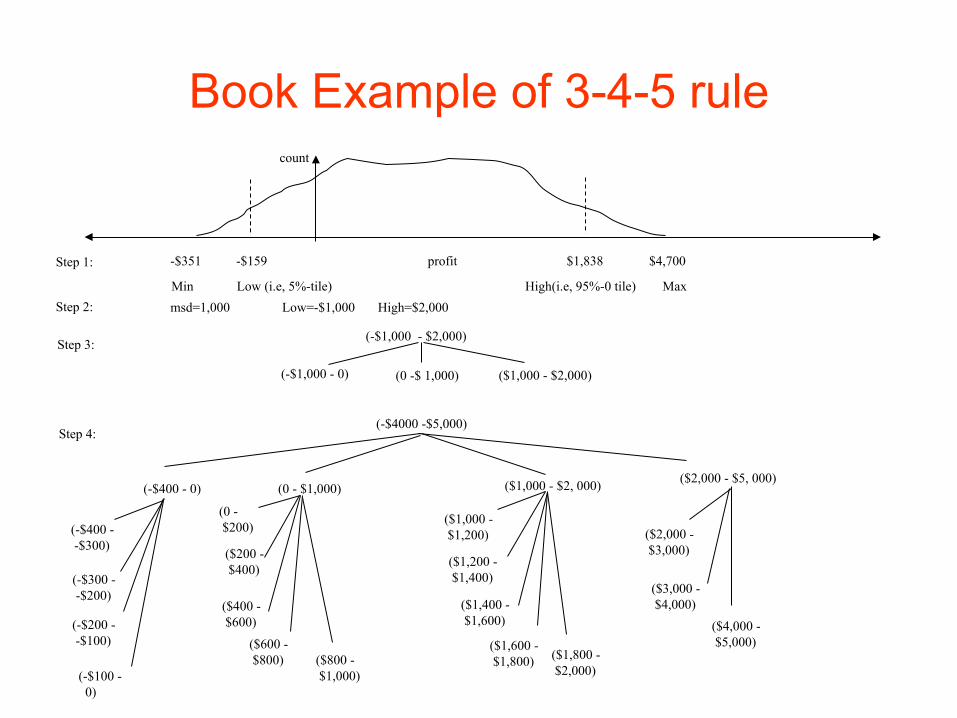
Book Example of 3-4-5 rule
(-$4000 -$5,000)
(-$400 - 0) (-$400 - -$300) (-$300 - -$200) (-$200 - -$100)
(-$100 - 0)
(0 - $1,000) (0 - $200) ($200 - $400)
($400 - $600)
($600 - $800) ($800 -
$1,000)
($2,000 - $5, 000)
($2,000 - $3,000)
($3,000 - $4,000)
($4,000 - $5,000)
($1,000 - $2, 000) ($1,000 - $1,200)
($1,200 - $1,400)
($1,400 - $1,600)
($1,600 - $1,800) ($1,800 -
$2,000)
msd=1,000 Low=-$1,000 High=$2,000 Step 2:
Step 4:
Step 1: -$351 -$159 profit $1,838 $4,700 Min Low (i.e, 5%-tile) High(i.e, 95%-0 tile) Max
count
(-$1,000 - $2,000)
(-$1,000 - 0) (0 -$ 1,000) Step 3:
($1,000 - $2,000)
Concept hierarchy generation for categorical data
• Concept hierarchy is: • Specification of a partial ordering of attributes
explicitly at the schema level by users or experts
• Specification of a portion of a hierarchy by explicit data grouping
• Specification of a set of attributes, but not of their partial ordering
• Specification of only a partial set of attributes
Concept Hierarchy Generation for Categorical Data
• Specification of a partial/total ordering of attributes explicitly at the schema level by users or experts – street < city < state < country
• Specification of a hierarchy for a set of values by explicit data grouping – {Urbana, Champaign, Chicago} < Illinois
• Specification of only a partial set of attributes – E.g., only street < city, not others
• Automatic generation of hierarchies (or attribute levels) by the analysis of the number of distinct values – E.g., for a set of attributes: {street, city, state, country}
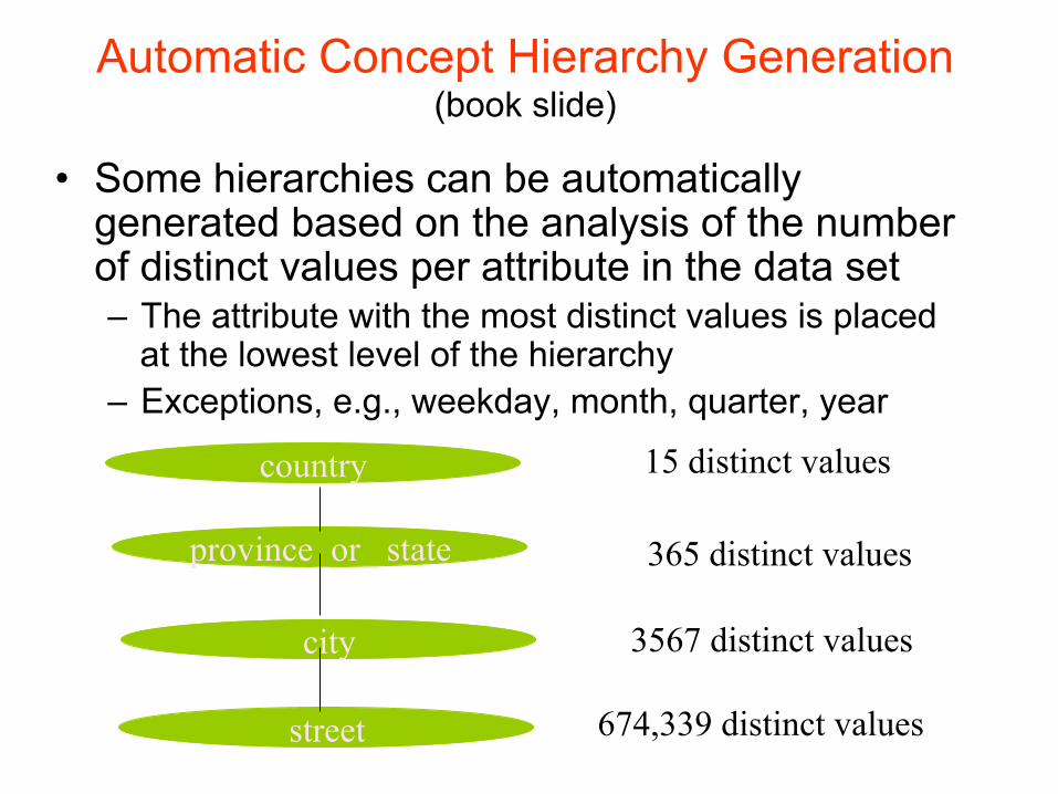
Automatic Concept Hierarchy Generation (book slide)
• Some hierarchies can be automatically generated based on the analysis of the number of distinct values per attribute in the data set – The attribute with the most distinct values is placed
at the lowest level of the hierarchy – Exceptions, e.g., weekday, month, quarter, year
country
province_or_ state
city
street
15 distinct values
365 distinct values
3567 distinct values
674,339 distinct values
Summary • Data preparation and preprocessing is a
big issue for both warehousing and mining
• Data preprocessing includes – Data cleaning and data integration
– Data reduction and atributes selection
– Discretization
• A lot a methods have been developed but still an active area of research


![Saad Nadeem and Arie Kaufman - arXiv.org e-Print …Further author information: Send correspondence to Saad Nadeem. E-mail: sanadeem@cs.stonybrook.edu 1 arXiv:1810.08998v1 [cs.CV]](https://static.fdocuments.us/doc/165x107/5f2e66a575b3b34c56424cbd/saad-nadeem-and-arie-kaufman-arxivorg-e-print-further-author-information-send.jpg)