CSE546:(Naïve(Bayes( Winter(2012( - courses.cs.washington.edu · Naïve Bayes for Digits (Binary...

CSE546: Naïve Bayes Winter 2012

Luke Ze=lemoyer

Slides adapted from Carlos Guestrin and Dan Klein

Supervised Learning: find f •  Given: Training set {(xi, yi) | i = 1 … n} •  Find: A good approximaMon to f : X à Y

Examples: what are X and Y ? •  Spam Detection

–  Map email to {Spam,Ham}

•  Digit recognition –  Map pixels to {0,1,2,3,4,5,6,7,8,9}

•  Stock Prediction –  Map new, historic prices, etc. to (the real numbers) !

ClassificaMon

Example: Spam Filter •  Input: email •  Output: spam/ham •  Setup:

–  Get a large collection of example emails, each labeled “spam” or “ham”

–  Note: someone has to hand label all this data!

–  Want to learn to predict labels of new, future emails

•  Features: The attributes used to make the ham / spam decision –  Words: FREE! –  Text Patterns: $dd, CAPS –  Non-text: SenderInContacts –  …

Dear Sir. First, I must solicit your confidence in this transaction, this is by virture of its nature as being utterly confidencial and top secret. …

TO BE REMOVED FROM FUTURE MAILINGS, SIMPLY REPLY TO THIS MESSAGE AND PUT "REMOVE" IN THE SUBJECT. 99 MILLION EMAIL ADDRESSES FOR ONLY $99

Ok, Iknow this is blatantly OT but I'm beginning to go insane. Had an old Dell Dimension XPS sitting in the corner and decided to put it to use, I know it was working pre being stuck in the corner, but when I plugged it in, hit the power nothing happened.

Example: Digit Recognition •  Input: images / pixel grids •  Output: a digit 0-9 •  Setup:

–  Get a large collection of example images, each labeled with a digit

–  Note: someone has to hand label all this data!

–  Want to learn to predict labels of new, future digit images

•  Features: The attributes used to make the digit decision –  Pixels: (6,8)=ON –  Shape Patterns: NumComponents,

AspectRatio, NumLoops –  …

0

1

2

1

??

Other Classification Tasks •  In classification, we predict labels y (classes) for inputs x

•  Examples: –  Spam detection (input: document, classes: spam / ham) –  OCR (input: images, classes: characters) –  Medical diagnosis (input: symptoms, classes: diseases) –  Automatic essay grader (input: document, classes: grades) –  Fraud detection (input: account activity, classes: fraud / no fraud) –  Customer service email routing –  … many more

•  Classification is an important commercial technology!

Lets take a probabilisMc approach!!!

•  Can we directly esMmate the data distribuMon P(X,Y)?

•  How do we represent these? How many parameters? –  Prior, P(Y):

•  Suppose Y is composed of k classes

–  Likelihood, P(X|Y): •  Suppose X is composed of n binary features

•  Complex model ! High variance with limited data!!!

mpg cylinders displacement horsepower weight acceleration modelyear maker

good 4 low low low high 75to78 asiabad 6 medium medium medium medium 70to74 americabad 4 medium medium medium low 75to78 europebad 8 high high high low 70to74 americabad 6 medium medium medium medium 70to74 americabad 4 low medium low medium 70to74 asiabad 4 low medium low low 70to74 asiabad 8 high high high low 75to78 america: : : : : : : :: : : : : : : :: : : : : : : :bad 8 high high high low 70to74 americagood 8 high medium high high 79to83 americabad 8 high high high low 75to78 americagood 4 low low low low 79to83 americabad 6 medium medium medium high 75to78 americagood 4 medium low low low 79to83 americagood 4 low low medium high 79to83 americabad 8 high high high low 70to74 americagood 4 low medium low medium 75to78 europebad 5 medium medium medium medium 75to78 europe

CondiMonal Independence •  X is condi(onally independent of Y given Z, if the probability distribuMon governing X is independent of the value of Y, given the value of Z

•  e.g., •  Equivalent to:

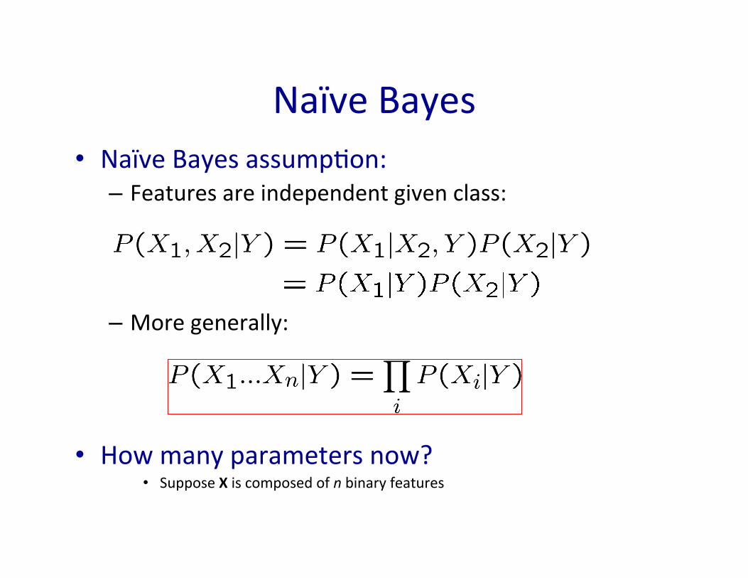
Naïve Bayes •  Naïve Bayes assumpMon:

–  Features are independent given class:

– More generally:

•  How many parameters now? •  Suppose X is composed of n binary features

The Naïve Bayes Classifier •  Given:

–  Prior P(Y) –  n condiMonally independent features X given the class Y

–  For each Xi, we have likelihood P(Xi|Y)

•  Decision rule:

If certain assumption holds, NB is optimal classifier! Will discuss at end of lecture!

Y

X1 Xn X2

A Digit Recognizer

•  Input: pixel grids

•  Output: a digit 0-9

Naïve Bayes for Digits (Binary Inputs) •  Simple version:

–  One feature Fij for each grid position <i,j> –  Possible feature values are on / off, based on whether intensity

is more or less than 0.5 in underlying image –  Each input maps to a feature vector, e.g.

–  Here: lots of features, each is binary valued

•  Naïve Bayes model:

•  Are the features independent given class? •  What do we need to learn?

Example Distributions

1 0.1 2 0.1 3 0.1 4 0.1 5 0.1 6 0.1 7 0.1 8 0.1 9 0.1 0 0.1

1 0.01 2 0.05 3 0.05 4 0.30 5 0.80 6 0.90 7 0.05 8 0.60 9 0.50 0 0.80

1 0.05 2 0.01 3 0.90 4 0.80 5 0.90 6 0.90 7 0.25 8 0.85 9 0.60 0 0.80

MLE for the parameters of NB •  Given dataset

–  Count(A=a,B=b) Ã number of examples where A=a and B=b

•  MLE for discrete NB, simply: –  Prior:

–  Likelihood:

µMLE ,σMLE = argmaxµ,σ

P (D | µ,σ)

= −N�

i=1

(xi − µ)

σ2= 0

= −N�

i=1

xi +Nµ = 0

= −N

σ+

N�

i=1

(xi − µ)2

σ3= 0

argmaxwln

�1

σ√2π

�N

+N�

j=1

−[tj −�

iwihi(xj)]2

2σ2

= argmaxw

N�

j=1

−[tj −�

iwihi(xj)]2

2σ2

= argminw

N�

j=1

[tj −�

i

wihi(xj)]2

P (Y = y) =Count(Y = y)�y� Count(Y = y�)

2


P (D | µ,σ)

= −N�

i=1

(xi − µ)

σ2= 0

= −N�

i=1

xi +Nµ = 0

= −N

σ+

N�

i=1

(xi − µ)2

σ3= 0

argmaxwln

�1

σ√2π

�N

+N�

j=1

−[tj −�

iwihi(xj)]2

2σ2

= argmaxw

N�

j=1

−[tj −�

iwihi(xj)]2

2σ2

= argminw

N�

j=1

[tj −�

i

wihi(xj)]2


2


P (D | µ,σ)

= −N�

i=1

(xi − µ)

σ2= 0

= −N�

i=1

xi +Nµ = 0

= −N

σ+

N�

i=1

(xi − µ)2

σ3= 0

argmaxwln

�1

σ√2π

�N

+N�

j=1

−[tj −�

iwihi(xj)]2

2σ2

= argmaxw

N�

j=1

−[tj −�

iwihi(xj)]2

2σ2

= argminw

N�

j=1

[tj −�

i

wihi(xj)]2


P (Xi = x|Y = y) =Count(Xi = x, Y = y)�x� Count(Xi = x�, Y = y)

2


P (D | µ,σ)

= −N�

i=1

(xi − µ)

σ2= 0

= −N�

i=1

xi +Nµ = 0

= −N

σ+

N�

i=1

(xi − µ)2

σ3= 0

argmaxwln

�1

σ√2π

�N

+N�

j=1

−[tj −�

iwihi(xj)]2

2σ2

= argmaxw

N�

j=1

−[tj −�

iwihi(xj)]2

2σ2

= argminw

N�

j=1

[tj −�

i

wihi(xj)]2



2

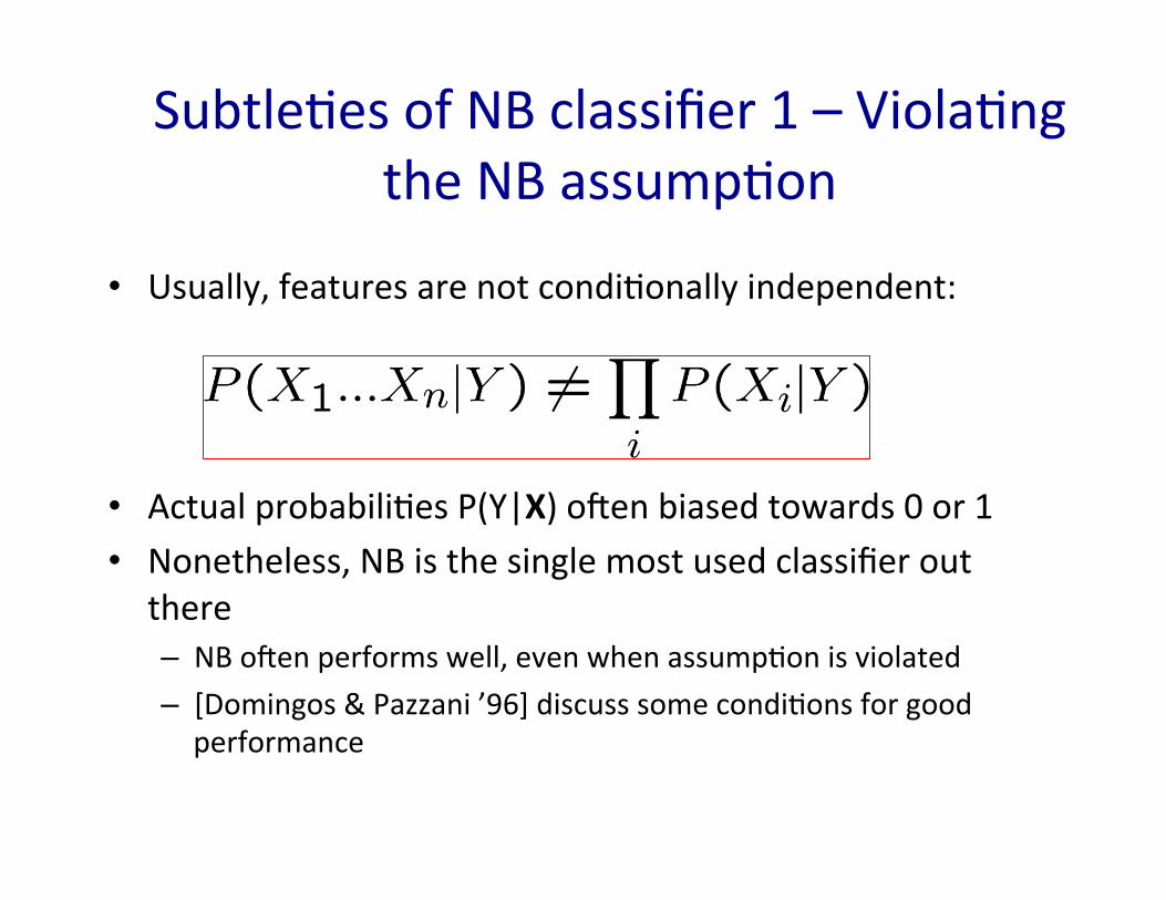
SubtleMes of NB classifier 1 – ViolaMng the NB assumpMon

•  Usually, features are not condiMonally independent:

•  Actual probabiliMes P(Y|X) ojen biased towards 0 or 1 •  Nonetheless, NB is the single most used classifier out

there –  NB ojen performs well, even when assumpMon is violated –  [Domingos & Pazzani ’96] discuss some condiMons for good performance

SubtleMes of NB classifier 2: Overfitting

2 wins!!

For Binary Features: We already know the answer!

•  MAP: use most likely parameter

•  Beta prior equivalent to extra observaMons for each feature

•  As N → 1, prior is “forgo=en” •  But, for small sample size, prior is important!

Brief Article

The Author

January 11, 2012

θ̂ = argmaxθ

lnP (D | θ)

ln θαH

d

dθlnP (D | θ) =

d

dθ[ln θαH (1− θ)αT ] =

d

dθ[αH ln θ + αT ln(1− θ)]

= αH

d

dθln θ + αT

d

dθln(1− θ) =

αH

θ− αT

1− θ= 0

δ ≥ 2e−2N�2 ≥ P (mistake)

ln δ ≥ ln 2− 2N�2

N ≥ ln(2/δ)

2�2

N ≥ ln(2/0.05)2× 0.12 ≈ 3.8

0.02= 190

P (θ) ∝ 1

P (θ | D) ∝ P (D | θ)

P (θ | D) ∝ θαH (1−θ)αT θβH−1(1−θ)βT−1 = θαH+βH−1(1−θ)αT+βt+1 = Beta(αH+βH , αT+βT )

αH + βH − 1αH + βH + αT + βT − 2

1

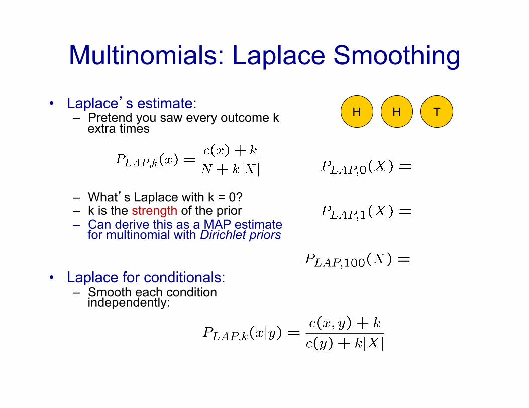
Multinomials: Laplace Smoothing •  Laplace’s estimate:

–  Pretend you saw every outcome k extra times

–  What’s Laplace with k = 0? –  k is the strength of the prior –  Can derive this as a MAP estimate

for multinomial with Dirichlet priors

•  Laplace for conditionals: –  Smooth each condition

independently:

H H T

Text classificaMon •  Classify e-‐mails

– Y = {Spam,NotSpam} •  Classify news arMcles

– Y = {what is the topic of the arMcle?} •  Classify webpages

– Y = {Student, professor, project, …}

•  What about the features X? – The text!

Features X are enMre document – Xi for ith word in arMcle

NB for Text classificaMon •  P(X|Y) is huge!!!

–  ArMcle at least 1000 words, X={X1,…,X1000} –  Xi represents ith word in document, i.e., the domain of Xi is enMre

vocabulary, e.g., Webster DicMonary (or more), 10,000 words, etc.

•  NB assumpMon helps a lot!!! –  P(Xi=xi|Y=y) is just the probability of observing word xi in a document on

topic y

Bag of words model •  Typical addiMonal assumpMon –

– Posi(on in document doesn’t ma;er: •  P(Xi=xi|Y=y) = P(Xk=xi|Y=y) (all posiMon have the same distribuMon)

–  “Bag of words” model – order of words on the page ignored

–  Sounds really silly, but ojen works very well!

When the lecture is over, remember to wake up the person sitting next to you in the lecture room.

Bag of words model

in is lecture lecture next over person remember room sitting the the the to to up wake when you

•  Typical addiMonal assumpMon –

– Posi(on in document doesn’t ma;er: •  P(Xi=xi|Y=y) = P(Xk=xi|Y=y) (all posiMon have the same distribuMon)

–  “Bag of words” model – order of words on the page ignored

–  Sounds really silly, but ojen works very well!

Bag of Words Approach

aardvark 0

about 2

all 2

Africa 1

apple 0

anxious 0

...

gas 1

...

oil 1

…

Zaire 0

NB with Bag of Words for text classificaMon •  Learning phase:

– Prior P(Y) •  Count how many documents from each topic (prior)

– P(Xi|Y) •  For each topic, count how many Mmes you saw word in documents of this topic (+ prior); remember this dist’n is shared across all posiMons i

•  Test phase: – For each document

•  Use naïve Bayes decision rule

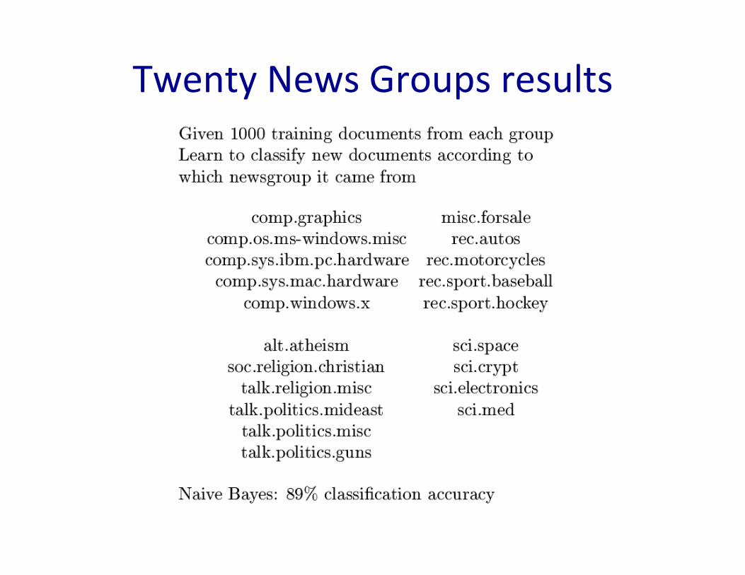
Twenty News Groups results

Learning curve for Twenty News Groups

What if we have conMnuous Xi ? Eg., character recogniMon: Xi is ith pixel Gaussian Naïve Bayes (GNB): SomeMmes assume variance •  is independent of Y (i.e., σi), •  or independent of Xi (i.e., σk) •  or both (i.e., σ)

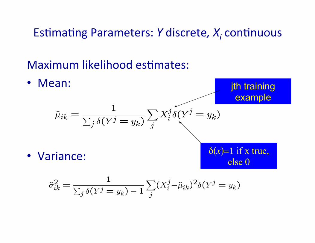
EsMmaMng Parameters: Y discrete, Xi conMnuous

Maximum likelihood esMmates: •  Mean:

•  Variance:

jth training example

δ(x)=1 if x true, else 0

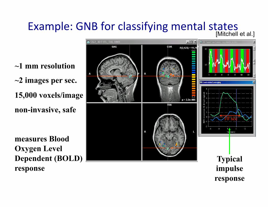
Example: GNB for classifying mental states

~1 mm resolution

~2 images per sec.

15,000 voxels/image

non-invasive, safe

measures Blood Oxygen Level Dependent (BOLD) response

Typical impulse response

10 sec

[Mitchell et al.]

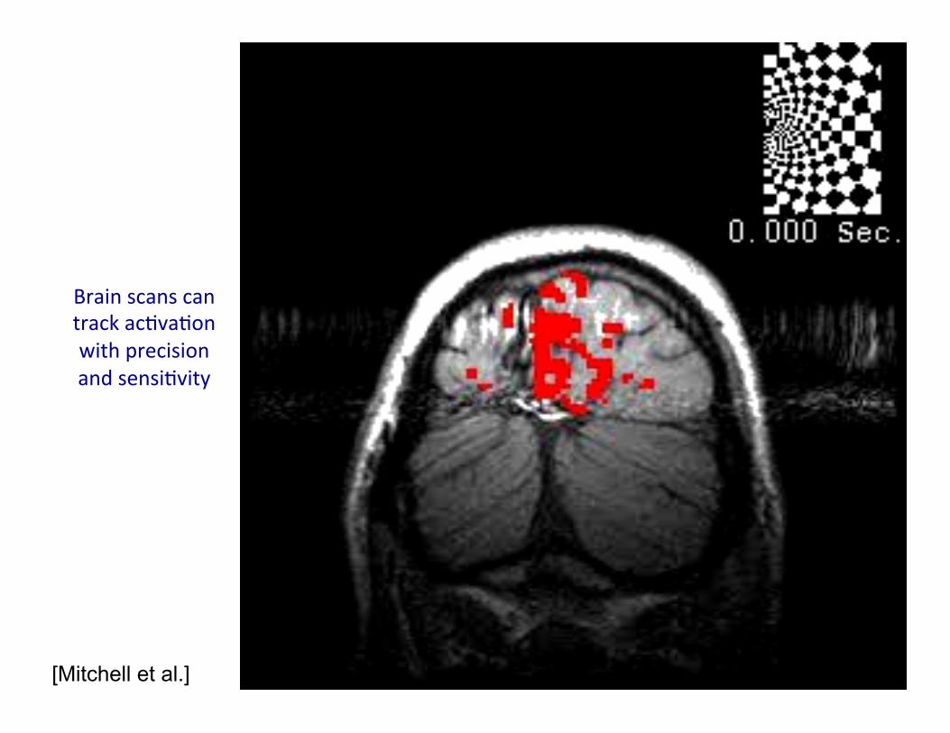
Brain scans can track acMvaMon with precision and sensiMvity

[Mitchell et al.]

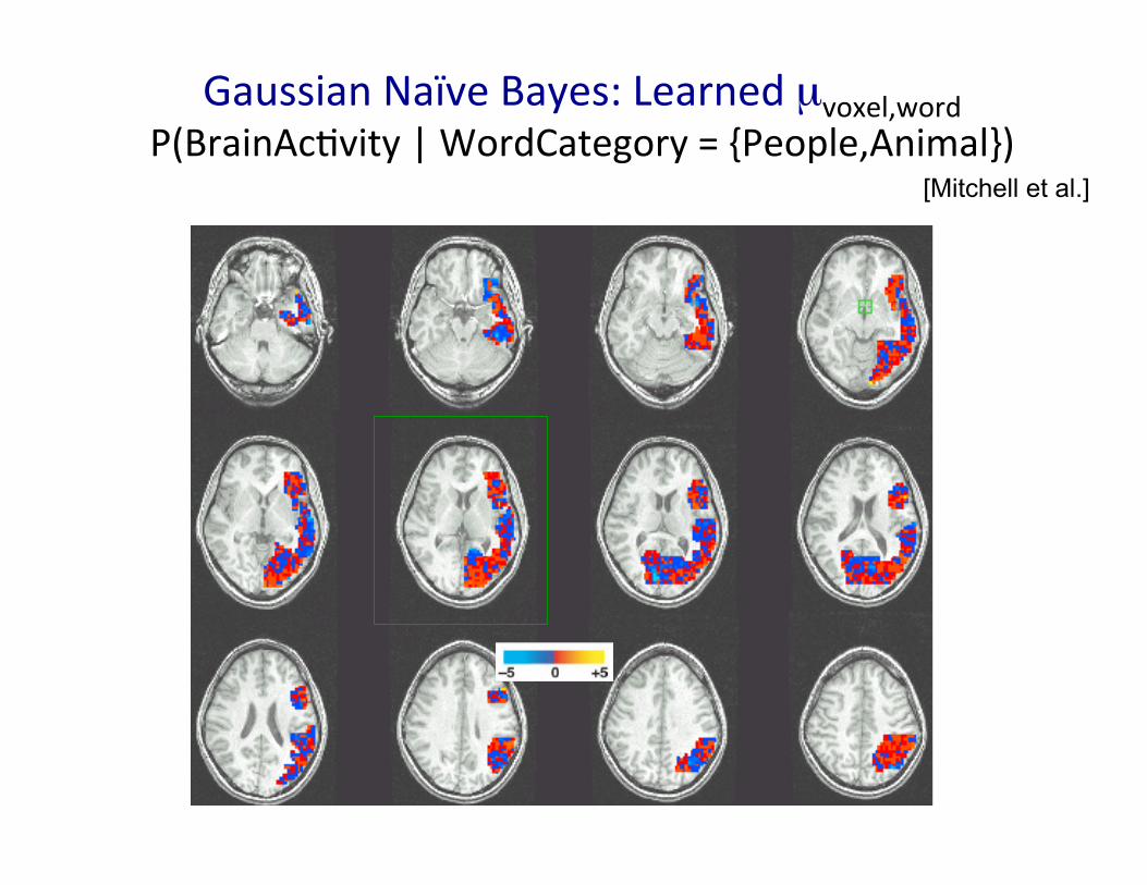
Gaussian Naïve Bayes: Learned µvoxel,word P(BrainAcMvity | WordCategory = {People,Animal})

[Mitchell et al.]

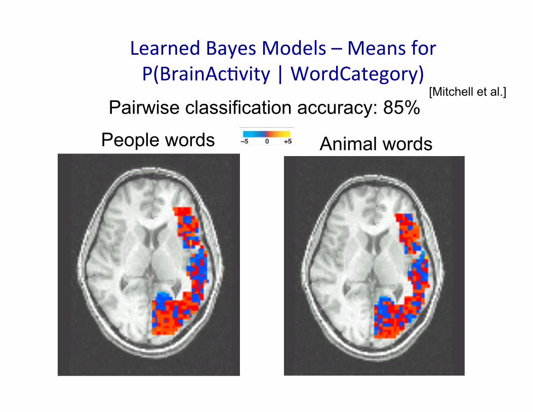
Learned Bayes Models – Means for P(BrainAcMvity | WordCategory)

Animal words People words

Pairwise classification accuracy: 85% [Mitchell et al.]

Bayes Classifier is OpMmal! •  Learn: h : X Y

– X – features – Y – target classes

•  Suppose: you know true P(Y|X): – Bayes classifier:

•  Why?


P (D | µ,σ)

= −N�

i=1

(xi − µ)

σ2= 0

= −N�

i=1

xi +Nµ = 0

= −N

σ+

N�

i=1

(xi − µ)2

σ3= 0

argmaxwln

�1

σ√2π

�N

+N�

j=1

−[tj −�

iwihi(xj)]2

2σ2

= argmaxw

N�

j=1

−[tj −�

iwihi(xj)]2

2σ2

= argminw

N�

j=1

[tj −�

i

wihi(xj)]2



hBayes(x) = argmaxy

P (Y = y|X = x)

2

OpMmal classificaMon •  Theorem:

– Bayes classifier hBayes is opMmal!

– Why?


P (D | µ,σ)

= −N�

i=1

(xi − µ)

σ2= 0

= −N�

i=1

xi +Nµ = 0

= −N

σ+

N�

i=1

(xi − µ)2

σ3= 0

argmaxwln

�1

σ√2π

�N

+N�

j=1

−[tj −�

iwihi(xj)]2

2σ2

= argmaxw

N�

j=1

−[tj −�

iwihi(xj)]2

2σ2

= argminw

N�

j=1

[tj −�

i

wihi(xj)]2



hBayes(x) = argmaxy

P (Y = y|X = x)

errortrue(hBayes) ≤ errortrue(h), ∀h

2


P (D | µ,σ)

= −N�

i=1

(xi − µ)

σ2= 0

= −N�

i=1

xi +Nµ = 0

= −N

σ+

N�

i=1

(xi − µ)2

σ3= 0

argmaxwln

�1

σ√2π

�N

+N�

j=1

−[tj −�

iwihi(xj)]2

2σ2

= argmaxw

N�

j=1

−[tj −�

iwihi(xj)]2

2σ2

= argminw

N�

j=1

[tj −�

i

wihi(xj)]2



hBayes(x) = argmaxy

P (Y = y|X = x)


ph(error) =

�

xph(error|x)p(x)dx

2


P (D | µ,σ)

= −N�

i=1

(xi − µ)

σ2= 0

= −N�

i=1

xi +Nµ = 0

= −N

σ+

N�

i=1

(xi − µ)2

σ3= 0

argmaxwln

�1

σ√2π

�N

+N�

j=1

−[tj −�

iwihi(xj)]2

2σ2

= argmaxw

N�

j=1

−[tj −�

iwihi(xj)]2

2σ2

= argminw

N�

j=1

[tj −�

i

wihi(xj)]2



hBayes(x) = argmaxy

P (Y = y|X = x)


ph(error) =

�

xph(error|x)p(x)dx

2


P (D | µ,σ)

= −N�

i=1

(xi − µ)

σ2= 0

= −N�

i=1

xi +Nµ = 0

= −N

σ+

N�

i=1

(xi − µ)2

σ3= 0

argmaxwln

�1

σ√2π

�N

+N�

j=1

−[tj −�

iwihi(xj)]2

2σ2

= argmaxw

N�

j=1

−[tj −�

iwihi(xj)]2

2σ2

= argminw

N�

j=1

[tj −�

i

wihi(xj)]2



hBayes(x) = argmaxy

P (Y = y|X = x)


ph(error) =

�

xph(error|x)p(x) =

�

x

�

yδ(h(x), y)p(y|x)p(x)

2

What you need to know about Naïve Bayes

•  Naïve Bayes classifier –  What’s the assumpMon –  Why we use it –  How do we learn it –  Why is Bayesian esMmaMon important

•  Text classificaMon –  Bag of words model

•  Gaussian NB –  Features are sMll condiMonally independent –  Each feature has a Gaussian distribuMon given class

•  OpMmal decision using Bayes Classifier

CSE546:(Naïve(Bayes( Winter(2012( - courses.cs.washington.edu · Naïve Bayes for Digits (Binary...

Documents

Transcript of CSE546:(Naïve(Bayes( Winter(2012( - courses.cs.washington.edu · Naïve Bayes for Digits (Binary...