CSE 544 Principles of Database Management Systems of Parallel Query Plan SELECT * FROM Orders o,...
73
CSE 544 Principles of Database Management Systems Magdalena Balazinska Winter 2015 Lecture 11 – Parallel DBMSs and MapReduce
Transcript of CSE 544 Principles of Database Management Systems of Parallel Query Plan SELECT * FROM Orders o,...

CSE 544 Principles of Database Management Systems
Magdalena Balazinska Winter 2015
Lecture 11 – Parallel DBMSs and MapReduce

CSE 544 - Magda Balazinska, Winter 2015 2
References
• Parallel Database Systems: The Future of High Performance Database Systems. Dave DeWitt and Jim Gray. Com. of the ACM. 1992. Also in Red Book 4th Ed. Sec. 1 and 2.
• MapReduce: Simplified Data Processing on Large Clusters. Jeffrey Dean and Sanjay Ghemawat. OSDI 2004. Sec. 1 - 4.
• Database management systems. Ramakrishnan and Gehrke.
Third Ed. Chapter 22.

How to Scale a DBMS?
3
Scale up
Scale out A more
powerful server
More servers

Why Do I Care About Scaling Transactions Per Second?
• Amazon • Facebook • Twitter • … your favorite Internet application…
• Goal is to scale OLTP workloads
• We will get back to this next week
CSE 544 - Magda Balazinska, Winter 2015 4

Why Do I Care About Scaling A Single Query?
• Goal is to scale OLAP workloads
• That means the analysis of massive datasets
CSE 544 - Magda Balazinska, Winter 2015 5

Today: Focus on Scaling a Single Query
CSE 544 - Magda Balazinska, Winter 2015 6

Science is Facing a Data Deluge!
• Astronomy: High-resolution, high-frequency sky surveys (SDSS, LSST)
• Medicine: ubiquitous digital records, MRI, ultrasound • Biology: lab automation, high-throughput sequencing • Oceanography: high-resolution models, cheap sensors,
satellites • Etc.
7
Data holds the promise to accelerate discovery
But analyzing all this data is a challenge
CSE 544 - Magda Balazinska, Winter 2015

Industry is Facing a Data Deluge!
• Clickstreams, search logs, network logs, social networking data, RFID data, etc.
• Examples: Facebook, Twitter, Google, Microsoft, Amazon, Walmart, etc.
8
Data holds the promise to deliver new and better services
But analyzing all this data is a challenge
CSE 544 - Magda Balazinska, Winter 2015

Big Data
• Companies, organizations, scientists have data that is too big, too fast, and too complex to be managed without changing tools and processes
• Relational algebra and SQL are easy to parallelize and parallel DBMSs have already been studied in the 80's!
CSE 544 - Magda Balazinska, Winter 2015 9

Data Analytics Companies
As a result, we are seeing an explosion of and a huge success of db analytics companies
• Greenplum founded in 2003 acquired by EMC in 2010; A parallel shared-nothing DBMS
• Vertica founded in 2005 and acquired by HP in 2011; A parallel, column-store shared-nothing DBMS
• DATAllegro founded in 2003 acquired by Microsoft in 2008; A parallel, shared-nothing DBMS
• Aster Data Systems founded in 2005 acquired by Teradata in 2011; A parallel, shared-nothing, MapReduce-based data processing system. SQL on top of MapReduce
• Netezza founded in 2000 and acquired by IBM in 2010. A parallel, shared-nothing DBMS.
CSE 544 - Magda Balazinska, Winter 2015 10

Two Approaches to Parallel Data Processing
• Parallel databases, developed starting with the 80s – For both OLTP (transaction processing) – And for OLAP (Decision Support Queries)
• MapReduce, first developed by Google, published in 2004 – Only for Decision Support Queries
Today we see convergence of the two approaches
11 CSE 544 - Magda Balazinska, Winter 2015

Parallel v.s. Distributed Databases
• Distributed database system (later): – Data is stored across several sites, each site managed by a
DBMS capable of running independently
• Parallel database system (today): – Improve performance through parallel implementation
12 CSE 544 - Magda Balazinska, Winter 2015

Parallel DBMSs
• Goal – Improve performance by executing multiple operations in parallel
• Key benefit
– Cheaper to scale than relying on a single increasingly more powerful processor
• Key challenge – Ensure overhead and contention do not kill performance
13 CSE 544 - Magda Balazinska, Winter 2015

Performance Metrics for Parallel DBMSs
Speedup • More processors è higher speed • Individual queries should run faster • Should do more transactions per second (TPS) • Fixed problem size overall, vary # of processors ("strong
scaling”)
14 CSE 544 - Magda Balazinska, Winter 2015

Linear v.s. Non-linear Speedup
# processors (=P)
Speedup
15 CSE 544 - Magda Balazinska, Winter 2015

Performance Metrics for Parallel DBMSs
Scaleup • More processors è can process more data • Fixed problem size per processor, vary # of processors
("weak scaling”) • Batch scaleup
– Same query on larger input data should take the same time • Transaction scaleup
– N-times as many TPS on N-times larger database – But each transaction typically remains small
16 CSE 544 - Magda Balazinska, Winter 2015

Linear v.s. Non-linear Scaleup
# processors (=P) AND data size
Batch Scaleup
×1 ×5 ×10 ×15
17 CSE 544 - Magda Balazinska, Winter 2015

Warning
• Be careful. Commonly used terms today: – “scale up” = use an increasingly more powerful server – “scale out” = use a larger number of servers
18 CSE 544 - Magda Balazinska, Winter 2015

Challenges to Linear Speedup and Scaleup
• Startup cost – Cost of starting an operation on many processors
• Interference – Contention for resources between processors
• Skew – Slowest processor becomes the bottleneck
19 CSE 544 - Magda Balazinska, Winter 2015

Architectures for Parallel Databases
20
From: Greenplum Database Whitepaper
SAN = “Storage Area Network” CSE 544 - Magda Balazinska, Winter 2015

Shared Memory
• Nodes share both RAM and disk • Dozens to hundreds of processors
Example: SQL Server runs on a single machine and can leverage many threads to get a query to run faster (see query plans)
• Easy to use and program • But very expensive to scale
CSE 544 - Magda Balazinska, Winter 2015 21

Shared Disk
• All nodes access the same disks • Found in the largest "single-box" (non-cluster)
multiprocessors
Oracle dominates this class of systems
Characteristics: • Also hard to scale past a certain point: existing
deployments typically have fewer than 10 machines
CSE 544 - Magda Balazinska, Winter 2015 22

Shared Nothing
• Cluster of machines on high-speed network • Called "clusters" or "blade servers” • Each machine has its own memory and disk: lowest
contention. NOTE: Because all machines today have many cores and many disks, then shared-nothing systems typically run many "nodes” on a single physical machine.
Characteristics: • Today, this is the most scalable architecture. • Most difficult to administer and tune.
23 CSE 544 - Magda Balazinska, Winter 2015 We discuss only Shared Nothing in class

In Class
• You have a parallel machine. Now what?
• How do you speed up your DBMS?
CSE 544 - Magda Balazinska, Winter 2015 24

Purchase
pid=pid
cid=cid
Customer
Product Purchase
pid=pid
cid=cid
Customer
Product
Approaches to Parallel Query Evaluation
• Inter-query parallelism – Each query runs on one processor – Only for OLTP queries
• Inter-operator parallelism – A query runs on multiple processors – An operator runs on one processor – For both OLTP and Decision Support
• Intra-operator parallelism – An operator runs on multiple processors – For both OLTP and Decision Support
CSE 544 - Magda Balazinska, Winter 2015
Purchase
pid=pid
cid=cid
Customer
Product
Purchase
pid=pid
cid=cid
Customer
Product
Purchase
pid=pid
cid=cid
Customer
Product
25 We study only intra-operator parallelism: most scalable

Horizontal Data Partitioning
• Relation R split into P chunks R0, …, RP-1, stored at the P nodes
• Block partitioned – Each group of k tuples go to a different node
• Hash based partitioning on attribute A: – Tuple t to chunk h(t.A) mod P
• Range based partitioning on attribute A: – Tuple t to chunk i if vi-1 < t.A < vi
26 CSE 544 - Magda Balazinska, Winter 2015

Uniform Data v.s. Skewed Data
• Let R(K,A,B,C); which of the following partition methods may result in skewed partitions?
• Block partition
• Hash-partition – On the key K – On the attribute A
• Range-partition – On the key K – On the attribute A
Uniform
Uniform
May be skewed
Assuming uniform hash function
E.g. when all records have the same value of the attribute A, then all records end up in the same partition
May be skewed Difficult to partition the range of A uniformly.
CSE 544 - Magda Balazinska, Winter 2015 27

28
Example from Teradata
AMP = unit of parallelism CSE 544 - Magda Balazinska, Winter 2015

Horizontal Data Partitioning
• All three choices are just special cases: – For each tuple, compute bin = f(t) – Different properties of the function f determine hash vs. range vs.
round robin vs. anything
29 CSE 544 - Magda Balazinska, Winter 2015

Parallel Selection
Compute σA=v(R), or σv1<A<v2(R)
• On a conventional database: cost = B(R)
• Q: What is the cost on a parallel database with P processors ? – Block partitioned – Hash partitioned – Range partitioned
30 CSE 544 - Magda Balazinska, Winter 2015

Parallel Selection
• Q: What is the cost on a parallel database with P nodes ?
• A: B(R) / P in all cases if cost is response time
• However, different processors do the work: – Block: all servers do the work – Hash: one server for σA=v(R), all for σv1<A<v2(R) – Range: some servers only
31 CSE 544 - Magda Balazinska, Winter 2015

Data Partitioning Revisited
What are the pros and cons ? • Block based partitioning
– Good load balance but always needs to read all the data
• Hash based partitioning – Good load balance – Can avoid reading all the data for equality selections
• Range based partitioning – Can suffer from skew (i.e., load imbalances) – Can help reduce skew by creating uneven partitions
32 CSE 544 - Magda Balazinska, Winter 2015

Parallel Group By: γA, sum(B)(R)
• Step 1: server i partitions chunk Ri using a hash function h(t.A) mod P: Ri0, Ri1, …, Ri,P-1
• Step 2: server i sends partition Rij to serve j
• Step 3: server j computes γA, sum(B) on R0j, R1j, …, RP-1,j
33 CSE 544 - Magda Balazinska, Winter 2015

Parallel GroupBy
γA,sum(C)(R) • If R is partitioned on A, then each node computes the
group-by locally • Otherwise, hash-partition R(K,A,B,C) on A, then compute
group-by locally:
34
R1 R2 RP . . .
R1’ R2’ RP’ . . .
Reshuffle R on attribute A
CSE 544 - Magda Balazinska, Winter 2015

Parallel Group By: γA, sum(B)(R)
• Can we do better? • Sum? • Count? • Avg? • Max? • Median?
35 CSE 544 - Magda Balazinska, Winter 2015

Parallel Group By: γA, sum(B)(R)
• Sum(B) = Sum(B0) + Sum(B1) + … + Sum(Bn) • Count(B) = Count(B0) + Count(B1) + … + Count(Bn) • Max(B) = Max(Max(B0), Max(B1), …, Max(Bn))
• Avg(B) = Sum(B) / Count(B)
• Median(B) =
36
distributive
algebraic
holistic
CSE 544 - Magda Balazinska, Winter 2015

Parallel Join: R ⋈A=B S
• Step 1 – For all servers in [0,k], server i partitions chunk Ri using a hash
function h(t.A) mod P: Ri0, Ri1, …, Ri,P-1 – For all servers in [k+1,P], server j partitions chunk Sj using a hash
function h(t.A) mod P: Sj0, Sj1, …, Rj,P-1
• Step 2:
– Server i sends partition Riu to server u – Server j sends partition Sju to server u
• Steps 3: Server u computes the join of Riu with Sju
37 CSE 544 - Magda Balazinska, Winter 2015

CSE 544 - Magda Balazinska, Winter 2015
Overall Architecture
38 From: Greenplum Database Whitepaper
SQL Query

39
Example of Parallel Query Plan
SELECT * FROM Orders o, Lines i WHERE o.item = i.item AND o.date = today()
join
select
scan scan
date = today()
o.item = i.item
Order o Item i
Find all orders from today, along with the items ordered
CSE 544 - Magda Balazinska, Winter 2015

40
Example Parallel Plan
Node 1 Node 2 Node 3
select date=today()
select date=today()
select date=today()
scan Order o
scan Order o
scan Order o
hash h(o.item)
hash h(o.item)
hash h(o.item)
Node 1 Node 2 Node 3
join
select
scan
date = today()
o.item = i.item
Order o
CSE 544 - Magda Balazinska, Winter 2015

41
Example Parallel Plan
Node 1 Node 2 Node 3
scan Item i
Node 1 Node 2 Node 3
hash h(i.item)
scan Item i
hash h(i.item)
scan Item i
hash h(i.item)
join
scan date = today()
o.item = i.item
Order o Item i
CSE 544 - Magda Balazinska, Winter 2015

42
Example Parallel Plan
Node 1 Node 2 Node 3
join join join o.item = i.item o.item = i.item o.item = i.item
contains all orders and all lines where hash(item) = 1
contains all orders and all lines where hash(item) = 2
contains all orders and all lines where hash(item) = 3
CSE 544 - Magda Balazinska, Winter 2015

Optimization for Small Relations
• When joining R and S • If |R| >> |S|
– Leave R where it is – Replicate entire S relation across nodes
• Sometimes called a “small join”
CSE 544 - Magda Balazinska, Winter 2015 43

Other Interesting Parallel Join Implementation
Problem of skew during join computation
– Some join partitions get more input tuples than others • Reason 1: Base data unevenly distributed across machines
– Because used a range-partition function – Or used hashing but some values are very popular
• Reason 2: Selection before join with different selectivities • Reason 3: Input data got unevenly rehashed (or otherwise
repartitioned before the join)
– Some partitions output more tuples than others
CSE 544 - Magda Balazinska, Winter 2015 44

Some Skew Handling Techniques 1. Use range- instead of hash-partitions
– Ensure that each range gets same number of tuples – Example: {1, 1, 1, 2, 3, 4, 5, 6 } à [1,2] and [3,6]
2. Create more partitions than nodes – And be smart about scheduling the partitions
3. Use subset-replicate (i.e., “skewedJoin”) – Given an extremely common value ‘v’ – Distribute R tuples with value v randomly across k nodes (R is
the build relation) – Replicate S tuples with value v to same k machines (S is the
probe relation)
CSE 544 - Magda Balazinska, Winter 2015 45

Parallel Dataflow Implementation
• Use relational operators unchanged
• Add a special shuffle operator – Handle data routing, buffering, and flow control – Inserted between consecutive operators in the query plan – Two components: ShuffleProducer and ShuffleConsumer – Producer pulls data from operator and sends to n consumers
• Producer acts as driver for operators below it in query plan – Consumer buffers input data from n producers and makes it
available to operator through getNext interface
46 CSE 544 - Magda Balazinska, Winter 2015

Map Reduce
• Google: [Dean 2004] • Open source implementation: Hadoop
• MapReduce = high-level programming model and implementation for large-scale parallel data processing
47 CSE 544 - Magda Balazinska, Winter 2015

MapReduce Motivation
• Not designed to be a DBMS • Designed to simplify task of writing parallel programs
– A simple programming model that applies to many large-scale computing problems
• Hides messy details in MapReduce runtime library: – Automatic parallelization – Load balancing – Network and disk transfer optimizations – Handling of machine failures – Robustness – Improvements to core library benefit all users of library!
CSE 544 - Magda Balazinska, Winter 2015 48 content in part from: Jeff Dean

Data Processing at Massive Scale
• Want to process petabytes of data and more
• Massive parallelism: – 100s, or 1000s, or 10000s servers (think data center) – Many hours
• Failure: – If medium-time-between-failure is 1 year – Then 10000 servers have one failure / hour
CSE 544 - Magda Balazinska, Winter 2015 49

Data Storage: GFS/HDFS
• MapReduce job input is a file
• Common implementation is to store files in a highly scalable file system such as GFS/HDFS – GFS: Google File System – HDFS: Hadoop File System
– Each data file is split into M blocks (64MB or more) – Blocks are stored on random machines & replicated – Files are append only
CSE 544 - Magda Balazinska, Winter 2015 50

51
Observation: Your favorite parallel algorithm…
Map
(Shuffle)
Reduce
CSE 544 - Magda Balazinska, Winter 2015

Typical Problems Solved by MR
• Read a lot of data • Map: extract something you care about from each record • Shuffle and Sort • Reduce: aggregate, summarize, filter, transform • Write the results
CSE 544 - Magda Balazinska, Winter 2015 52
Outline stays the same, map and reduce change to fit the problem
slide source: Jeff Dean

Data Model
Files !
A file = a bag of (key, value) pairs
A MapReduce program: • Input: a bag of (inputkey, value)pairs • Output: a bag of (outputkey, value)pairs
53 CSE 544 - Magda Balazinska, Winter 2015

Step 1: the MAP Phase
User provides the MAP-function: • Input: (input key, value) • Ouput: bag of (intermediate key, value)
System applies map function in parallel to all (input key, value) pairs in the input file
54 CSE 544 - Magda Balazinska, Winter 2015

Step 2: the REDUCE Phase
User provides the REDUCE function: • Input: (intermediate key, bag of values)
• Output (original MR paper): bag of output (values) • Output (Hadoop): bag of (output key, values)
System groups all pairs with the same intermediate key, and passes the bag of values to the REDUCE function
55 CSE 544 - Magda Balazinska, Winter 2015

Example
• Counting the number of occurrences of each word in a large collection of documents
• Each Document – The key = document id (did) – The value = set of words (word)
map(String key, String value): // key: document name // value: document contents for each word w in value:
EmitIntermediate(w, “1”);
reduce(String key, Iterator values): // key: a word // values: a list of counts int result = 0; for each v in values:
result += ParseInt(v); Emit(AsString(result));
56 CSE 544 - Magda Balazinska, Winter 2015

MAP REDUCE
(w1,1)
(w2,1)
(w3,1)
…
(w1,1)
(w2,1)
…
(did1,v1)
(did2,v2)
(did3,v3)
. . . .
(w1, (1,1,1,…,1))
(w2, (1,1,…))
(w3,(1…))
…
…
…
…
(w1, 25)
(w2, 77)
(w3, 12)
…
…
…
…
Shuffle
57 CSE 544 - Magda Balazinska, Winter 2015

Jobs v.s. Tasks
• A MapReduce Job – One single “query”, e.g. count the words in all docs – More complex queries may consist of multiple jobs
• A Map Task, or a Reduce Task – A group of instantiations of the map-, or reduce-function, which
are scheduled on a single worker
CSE 544 - Magda Balazinska, Winter 2015 58

Workers
• A worker is a process that executes one task at a time • Typically there is one worker per processor, hence 4 or 8
per node
• Often talk about “slots” – E.g., Each server has 2 map slots and 2 reduce slots
CSE 544 - Magda Balazinska, Winter 2015 59

MAP Tasks REDUCE Tasks
(w1,1)
(w2,1)
(w3,1)
…
(w1,1)
(w2,1)
…
(did1,v1)
(did2,v2)
(did3,v3)
. . . .
(w1, (1,1,1,…,1))
(w2, (1,1,…))
(w3,(1…))
…
…
…
…
(w1, 25)
(w2, 77)
(w3, 12)
…
…
…
…
Shuffle
60

Parallel MapReduce Details
CSE 544 - Magda Balazinska, Winter 2015 61
Map
(Shuffle)
Reduce
Data not necessarily local
Intermediate data goes to local disk
Output to disk, replicated in cluster
File system: GFS or HDFS
Task
Task

MapReduce Implementation
• There is one master node • Input file gets partitioned further into M’ splits
– Each split is a contiguous piece of the input file
• Master assigns workers (=servers) to the M’ map tasks, keeps track of their progress
• Workers write their output to local disk • Output of each map task is partitioned into R regions • Master assigns workers to the R reduce tasks • Reduce workers read regions from the map workers’
local disks
CSE 544 - Magda Balazinska, Winter 2015 62
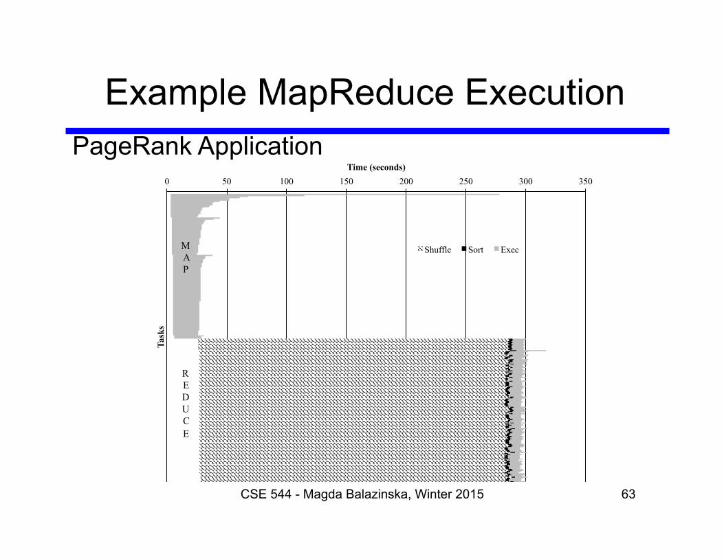
Example MapReduce Execution
CSE 544 - Magda Balazinska, Winter 2015 63
0 50 100 150 200 250 300 350 Time (seconds)
Task
s
Shuffle Sort Exec M A P
R E D U C E
PageRank Application

Example: CloudBurst
CloudBurst. Lake Washington Dataset (1.1GB). 80 Mappers 80 Reducers.
Map Reduce Sort Shuffle Slot ID
Time 64 CSE 544 - Magda Balazinska, Winter 2015

Local storage `
MapReduce Phases
65 CSE 544 - Magda Balazinska, Winter 2015

Interesting Implementation Details
• Worker failure: – Master pings workers periodically, – If down then reassigns its task to another worker – (≠ a parallel DBMS restarts whole query)
• How many map and reduce tasks: – Larger is better for load balancing – But more tasks also add overheads – (≠ parallel DBMS spreads ops across all nodes)
CSE 544 - Magda Balazinska, Winter 2015 66

MapReduce Granularity Illustration
0 1 2 3 4 5 6 7 8 9
10
Rel
ativ
e R
untim
e
Astro Seaflow
Coarse Fine Finer Finest Manual SkewReduce 14.1 8.8 4.1 5.7 2.0 1.6 87.2 63.1 77.7 98.7 - 14.1
Hours Minutes
67 CSE 544 - Magda Balazinska, Winter 2015

Interesting Implementation Details
Backup tasks: • Straggler = a machine that takes unusually long time to
complete one of the last tasks. Eg: – Bad disk forces frequent correctable errors (30MB/s à 1MB/s) – The cluster scheduler has scheduled other tasks on that machine
• Stragglers are a main reason for slowdown • Solution: pre-emptive backup execution of the last few
remaining in-progress tasks
CSE 544 - Magda Balazinska, Winter 2015 68

Parallel DBMS vs MapReduce
• Parallel DBMS – Relational data model and schema – Declarative query language: SQL – Many pre-defined operators: relational algebra – Can easily combine operators into complex queries – Query optimization, indexing, and physical tuning – Streams data from one operator to the next without blocking – Can do more than just run queries: Data management
• Updates and transactions, constraints, security, etc.
69 CSE 544 - Magda Balazinska, Winter 2015

Parallel DBMS vs MapReduce
• MapReduce – Data model is a file with key-value pairs! – No need to “load data” before processing it – Easy to write user-defined operators – Can easily add nodes to the cluster (no need to even restart) – Uses less memory since processes one key-group at a time – Intra-query fault-tolerance thanks to results on disk – Intermediate results on disk also facilitate scheduling – Handles adverse conditions: e.g., stragglers – Arguably more scalable… but also needs more nodes!
70 CSE 544 - Magda Balazinska, Winter 2015

Declarative Languages on MR
• PIG Latin (Yahoo!) – New language, like Relational Algebra – Open source
• HiveQL (Facebook) – SQL-like language – Open source
• SQL / Tenzing (Google) – SQL on MR – Proprietary
71 CSE 544 - Magda Balazinska, Winter 2015

Example: Pig system
72
Pig Latin program
A = LOAD 'file1' AS (sid,pid,mass,px:double); B = LOAD 'file2' AS (sid,pid,mass,px:double); C = FILTER A BY px < 1.0; D = JOIN C BY sid, B BY sid; STORE g INTO 'output.txt';
Ensemble of MapReduce jobs

MapReduce State
• Lots of extensions to address limitations – Capabilities to write DAGs of MapReduce jobs – Declarative languages – Ability to read from structured storage (e.g., indexes) – Etc.
• Most companies use both types of engines • Increased integration of both engines
CSE 544 - Magda Balazinska, Winter 2015 73