CSE 422 Notes, Set 4dennisp/cse422/Slides/set4-1_student.pdfThese slides contain materials provided...
26
1 CSE 422 - Phillips CSE 422 Notes, Set 4 These slides contain materials provided with the text: Computer Networking: A Top Down Approach,5th edition, by Jim Kurose and Keith Ross, Addison-Wesley, April 2009. Additional figures are repeated, with permission, from Computer Networks, 2nd through 4th Editions, by A. S. Tanenbaum, Prentice Hall. Some figures are repeated from an OPNET Technologies presentation by Dmitri Bertsekas and course notes from Rutgers University. The remainder of the materials were developed by Philip McKinley and Dennis Phillips at Michigan State University Network Layer CSE 422 - Phillips Assignment: Read Chapter 4 of Kurose-Ross Transport Layer
Transcript of CSE 422 Notes, Set 4dennisp/cse422/Slides/set4-1_student.pdfThese slides contain materials provided...
1
CSE 422 - Phillips
CSE 422 Notes, Set 4 These slides contain materials provided with the text:
Computer Networking: A Top Down Approach,5th edition, by Jim Kurose and Keith Ross, Addison-Wesley, April 2009.
Additional figures are repeated, with permission, from Computer Networks, 2nd through 4th Editions, by A. S. Tanenbaum, Prentice Hall.
Some figures are repeated from an OPNET Technologies presentation by Dmitri Bertsekas and course notes from Rutgers University.
The remainder of the materials were developed by Philip McKinley and Dennis Phillips at Michigan State University
Network Layer
CSE 422 - Phillips
Assignment:
Read Chapter 4 of Kurose-Ross
Transport Layer
2
CSE 422 - Phillips Network Layer
Chapter 4: Network Layer
Introduction (forwarding and routing)
Review of queueing theory
Routing algorithms Link state, Distance Vector
Router design and operation
IP: Internet Protocol IPv4 (datagram format, addressing, ICMP, NAT)
Ipv6
Routing in the Internet Autonomous Systems
Routing protocols (RIP, OSPF, BGP)
CSE 422 - Phillips Network Layer
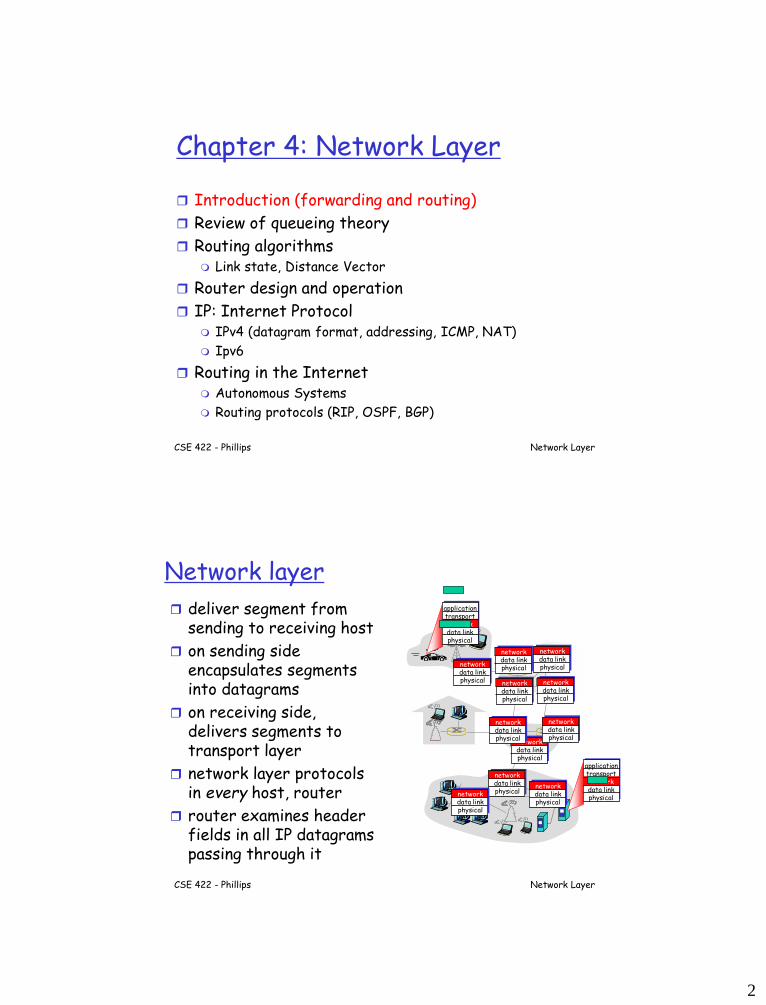
Network layer
deliver segment from sending to receiving host
on sending side encapsulates segments into datagrams
on receiving side, delivers segments to transport layer
network layer protocols in every host, router
router examines header fields in all IP datagrams passing through it
applicationtransportnetworkdata linkphysical
applicationtransportnetworkdata linkphysical
networkdata linkphysical network
data linkphysical
networkdata linkphysical
networkdata linkphysical
networkdata linkphysical
networkdata linkphysical
networkdata linkphysical
networkdata linkphysical
networkdata linkphysical
networkdata linkphysicalnetwork
data linkphysical
3
CSE 422 - Phillips Network Layer
Two Key Network-Layer Functions
routing: determine route taken by packets from source to destination
Distributed routing in the Internet
Could also be centralized (drawbacks?)
forwarding: move packets from router’s input to appropriate router output
CSE 422 - Phillips Network Layer
1
23
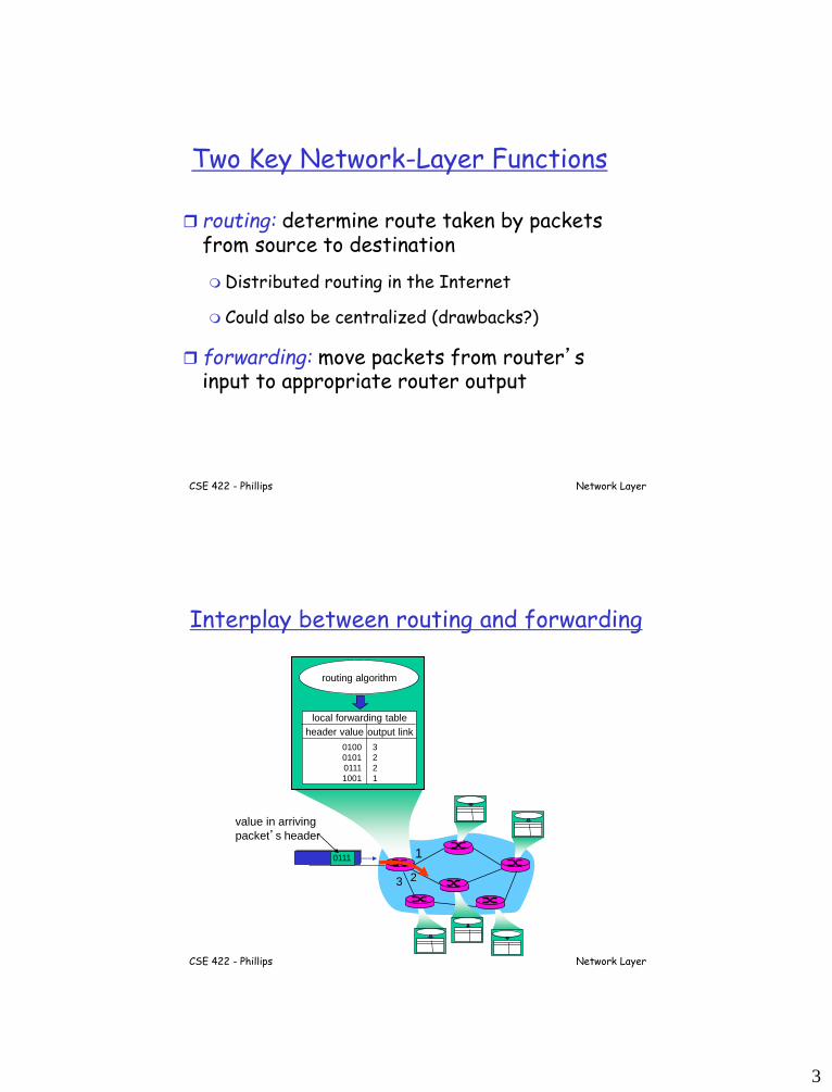
0111
value in arriving
packet’s header
routing algorithm
local forwarding table
header value output link
0100
0101
0111
1001
3
2
2
1
Interplay between routing and forwarding
4
CSE 422 - Phillips Network Layer
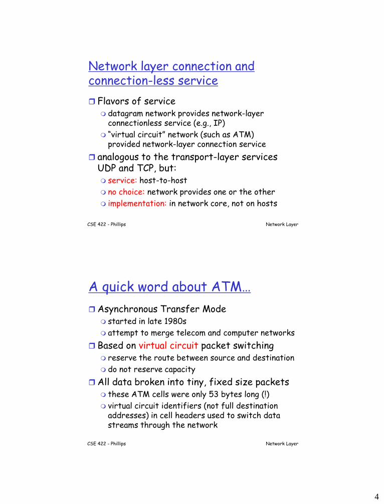
Network layer connection and connection-less service
Flavors of service datagram network provides network-layer
connectionless service (e.g., IP)
“virtual circuit” network (such as ATM) provided network-layer connection service
analogous to the transport-layer services UDP and TCP, but: service: host-to-host
no choice: network provides one or the other
implementation: in network core, not on hosts
CSE 422 - Phillips
A quick word about ATM…
Asynchronous Transfer Mode started in late 1980s
attempt to merge telecom and computer networks
Based on virtual circuit packet switching reserve the route between source and destination
do not reserve capacity
All data broken into tiny, fixed size packets these ATM cells were only 53 bytes long (!)
virtual circuit identifiers (not full destination addresses) in cell headers used to switch data streams through the network
Network Layer
5
CSE 422 - Phillips
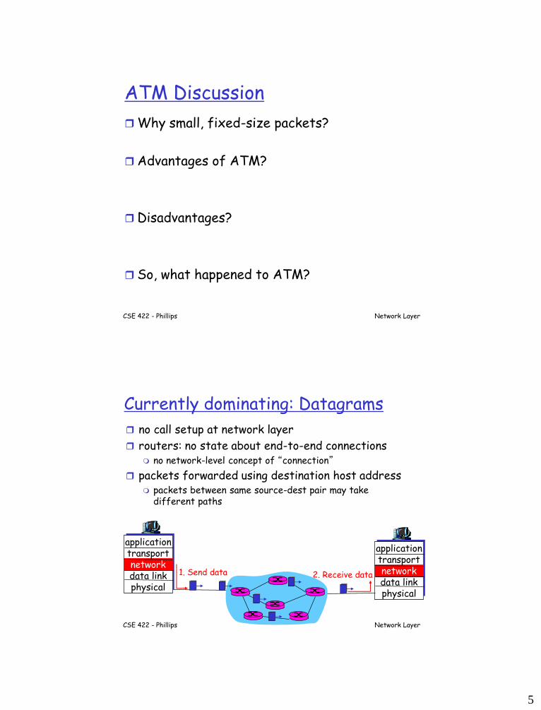
ATM Discussion
Why small, fixed-size packets?
Advantages of ATM?
Disadvantages?
So, what happened to ATM?
Network Layer
CSE 422 - Phillips Network Layer
Currently dominating: Datagrams
no call setup at network layer
routers: no state about end-to-end connections no network-level concept of “connection”
packets forwarded using destination host address packets between same source-dest pair may take
different paths
applicationtransportnetworkdata linkphysical
applicationtransportnetworkdata linkphysical
1. Send data 2. Receive data
6
CSE 422 - Phillips
Datagram Issues
Since capacity is not reserved, datagrams compete for network resources: Communication links
Router buffers
Bursty traffic creates periods of high and low demand, resulting in queueing of datagrams at network routers.
Performance depends on complex interactions.
Advent of packet switching produced need to: analyze performance of existing networks
predict performance of new designs
Network Layer
CSE 422 - Phillips Network Layer
Chapter 4: Network Layer
Introduction (forwarding and routing)
Review of queueing theory
Routing algorithms Link state, Distance Vector
Router design and operation
IP: Internet Protocol IPv4 (datagram format, addressing, ICMP, NAT)
Ipv6
Routing in the Internet Autonomous Systems
Routing protocols (RIP, OSPF, BGP)
7
CSE 422 - Phillips
Brief Review of Queueing Theory
Definition: Any system in which arrivals place demands upon a finite-capacity resource may be termed a queueing system.
Applications of Queueing Theory analysis of computer networks
telephone switching systems
customer service centers
automobile traffic control
almost any application involving entities waiting for and receiving service
Network Layer
CSE 422 - Phillips
For studying computer networks…
View network as collections of queues First-in, first-out (FIFO) data structures
Queueing theory provides probabilistic analysis of these queues
Examples: Average queue length Average waiting (and service) time Probability that queue is at a certain length Probability of queue overflow (packets will be
dropped)
Network Layer
8
CSE 422 - Phillips
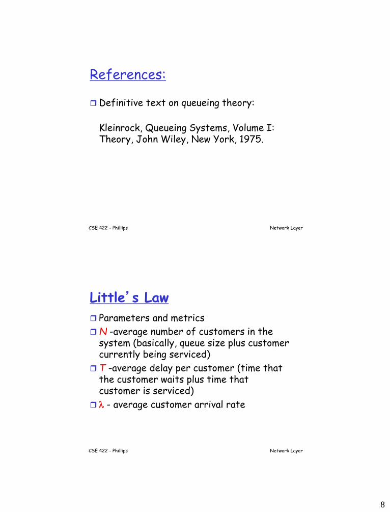
References:
Definitive text on queueing theory:
Kleinrock, Queueing Systems, Volume I: Theory, John Wiley, New York, 1975.
Network Layer
CSE 422 - Phillips
Little’s Law
Parameters and metrics
N -average number of customers in the system (basically, queue size plus customer currently being serviced)
T -average delay per customer (time that the customer waits plus time that customer is serviced)
- average customer arrival rate
Network Layer
9
CSE 422 - Phillips
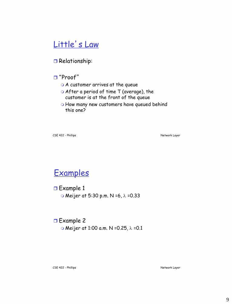
Little’s Law
Relationship:
“Proof” A customer arrives at the queue
After a period of time T (average), the customer is at the front of the queue
How many new customers have queued behind this one?
Network Layer
CSE 422 - Phillips
Examples
Example 1 Meijer at 5:30 p.m. N =6, =0.33
Example 2 Meijer at 1:00 a.m. N =0.25, =0.1
Network Layer
10
CSE 422 - Phillips
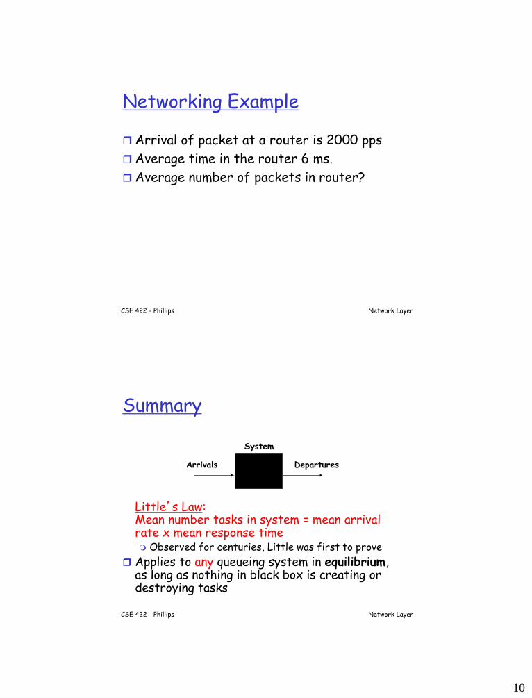
Networking Example
Arrival of packet at a router is 2000 pps
Average time in the router 6 ms.
Average number of packets in router?
Network Layer
CSE 422 - Phillips
Summary
Little’s Law: Mean number tasks in system = mean arrival rate x mean response time Observed for centuries, Little was first to prove
Applies to any queueing system in equilibrium, as long as nothing in black box is creating or destroying tasks
Network Layer
Arrivals Departures
System
11
CSE 422 - Phillips
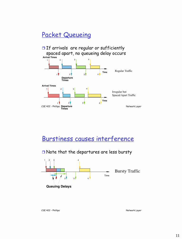
Packet Queueing
If arrivals are regular or sufficiently spaced apart, no queueing delay occurs
Network Layer
Regular Traffic
Irregular but
Spaced Apart Traffic
CSE 422 - Phillips
Burstiness causes interference
Note that the departures are less bursty
Network Layer
12
CSE 422 - Phillips
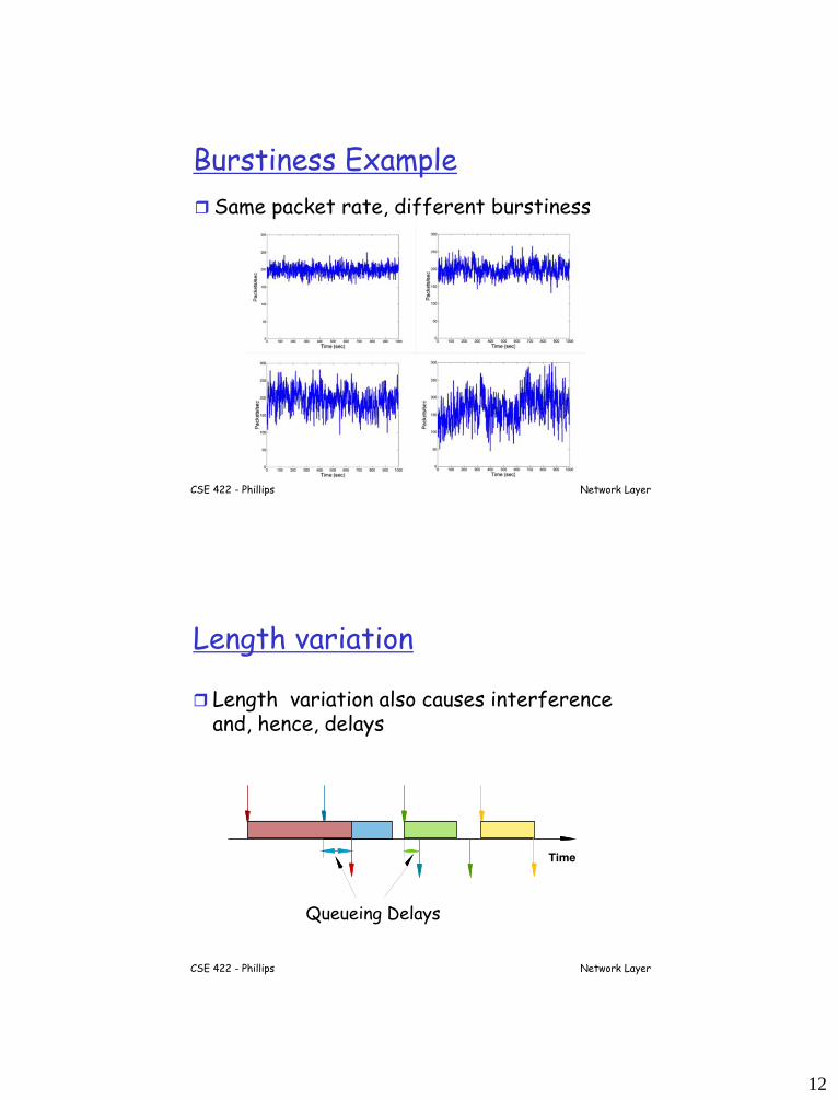
Burstiness Example
Same packet rate, different burstiness
Network Layer
CSE 422 - Phillips
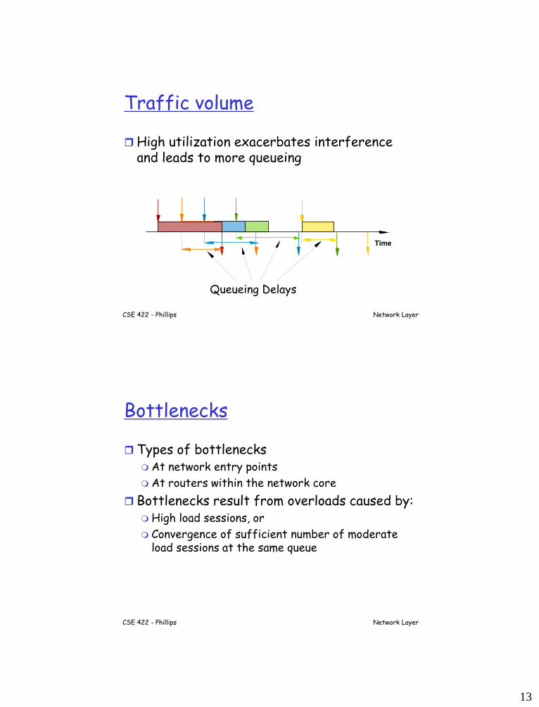
Length variation
Length variation also causes interference and, hence, delays
Network Layer
Queueing Delays
13
CSE 422 - Phillips
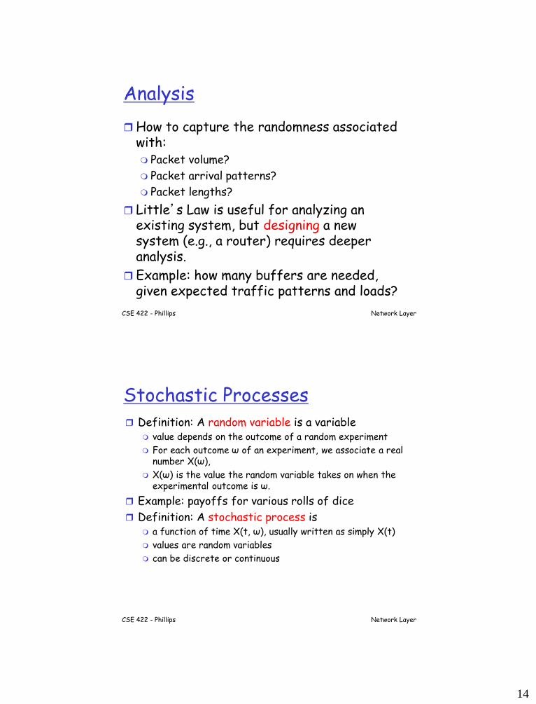
Traffic volume
High utilization exacerbates interference and leads to more queueing
Network Layer
Queueing Delays
CSE 422 - Phillips
Bottlenecks
Types of bottlenecks At network entry points
At routers within the network core
Bottlenecks result from overloads caused by: High load sessions, or
Convergence of sufficient number of moderate load sessions at the same queue
Network Layer
14
CSE 422 - Phillips
Analysis
How to capture the randomness associated with: Packet volume?
Packet arrival patterns?
Packet lengths?
Little’s Law is useful for analyzing an existing system, but designing a new system (e.g., a router) requires deeper analysis.
Example: how many buffers are needed, given expected traffic patterns and loads?
Network Layer
CSE 422 - Phillips
Stochastic Processes Definition: A random variable is a variable
value depends on the outcome of a random experiment
For each outcome ω of an experiment, we associate a real number X(ω),
X(ω) is the value the random variable takes on when the experimental outcome is ω.
Example: payoffs for various rolls of dice
Definition: A stochastic process is a function of time X(t, ω), usually written as simply X(t)
values are random variables
can be discrete or continuous
Network Layer
15
CSE 422 - Phillips
Examples
Dow Jones closing averages.
Number of cars that have pulled into Meijer’s parking lot by time t.
Number of packets generated by a host by time t.
Number of packets arriving at a router by time t.
Network Layer
CSE 422 - Phillips
Poisson Processes
Definition: A stochastic process {A(t)|t > 0} taking on nonnegative integer values is said to be a Poisson process with rate if
A(t) is a counting process that represents the total number of arrivals that have occurred from 0 to time t.
The numbers of arrivals that occur in disjoint time intervals are independent.
The number of arrivals in any interval of length is Poisson distributed with parameter
P {A(t + ) − A(t) = n} =
for n =0, 1, 2, ...
Network Layer
16
CSE 422 - Phillips
Example Customers join Meijer’s checkout lane with an average arrival
rate of one customer every 2 minutes. What is the probability that exactly 2 customers join the queue in a period of 5 minutes?
What is the probability that no customers join the queue in this time?
Network Layer
CSE 422 - Phillips
Poisson Process Properties
Interarrival times are independent and exponentially distributed with parameter
P{n≤ t} = 1 − e−t, t ≥ 0
Why?
Graph?
Network Layer
17
CSE 422 - Phillips
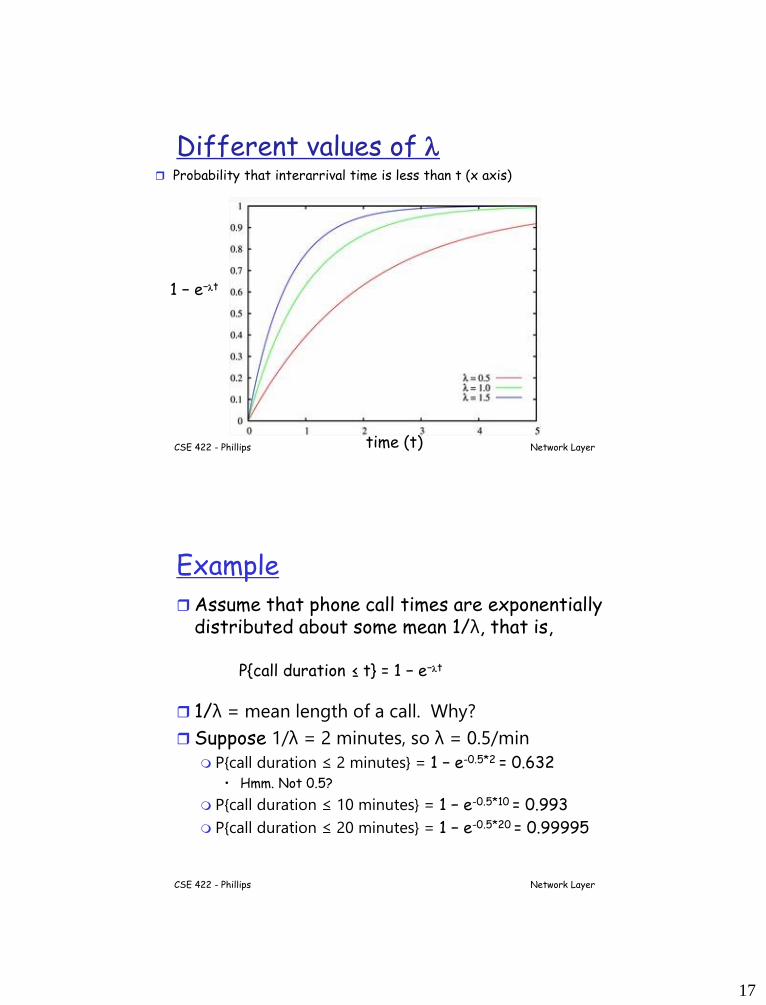
Different values of Probability that interarrival time is less than t (x axis)
Network Layer
1 − e−t
time (t)
CSE 422 - Phillips
Example
Assume that phone call times are exponentially distributed about some mean 1/λ, that is,
P{call duration ≤ t} = 1 − e−t
1/λ = mean length of a call. Why?
Suppose 1/λ = 2 minutes, so λ = 0.5/min
P{call duration ≤ 2 minutes} = 1 − e-0.5*2 = 0.632• Hmm. Not 0.5?
P{call duration ≤ 10 minutes} = 1 − e-0.5*10 = 0.993
P{call duration ≤ 20 minutes} = 1 − e-0.5*20 = 0.99995
Network Layer
18
CSE 422 - Phillips
Consider this situation:
You are attending a retreat in a remote location No cell phone service !?!
Two public phones are available in the lobby of the lodge
You need to make a call, but both phones are currently busy A person nearby tells you that one person just
started his/her call, while the other has been on the phone for 30 minutes.
Which phone should you wait for?
Network Layer
CSE 422 - Phillips
The Markov Property
The exponential distribution is said to be:
Specifically,
Why does this property hold?
Network Layer
19
CSE 422 - Phillips
Queueing System Characterization
Five components
Interarrival-time pdf
Service-time pdf
Number of servers
Queuing discipline, that is, how customers are taken from the queue
Number of buffers (for customers)
We will consider infinite-buffer, single-server systems, using a FIFO queueing discipline
Network Layer
CSE 422 - Phillips
Notation
Notation for first 3 components: A/B/m, with A and B chosen from M -Markov (exponential pdf)
D -Deterministic (all customers have same value)
G -General (arbitrary pdf)
Example of M/M/1?
Example of M/D/1?
Example of D/D/1?
Network Layer
20
CSE 422 - Phillips
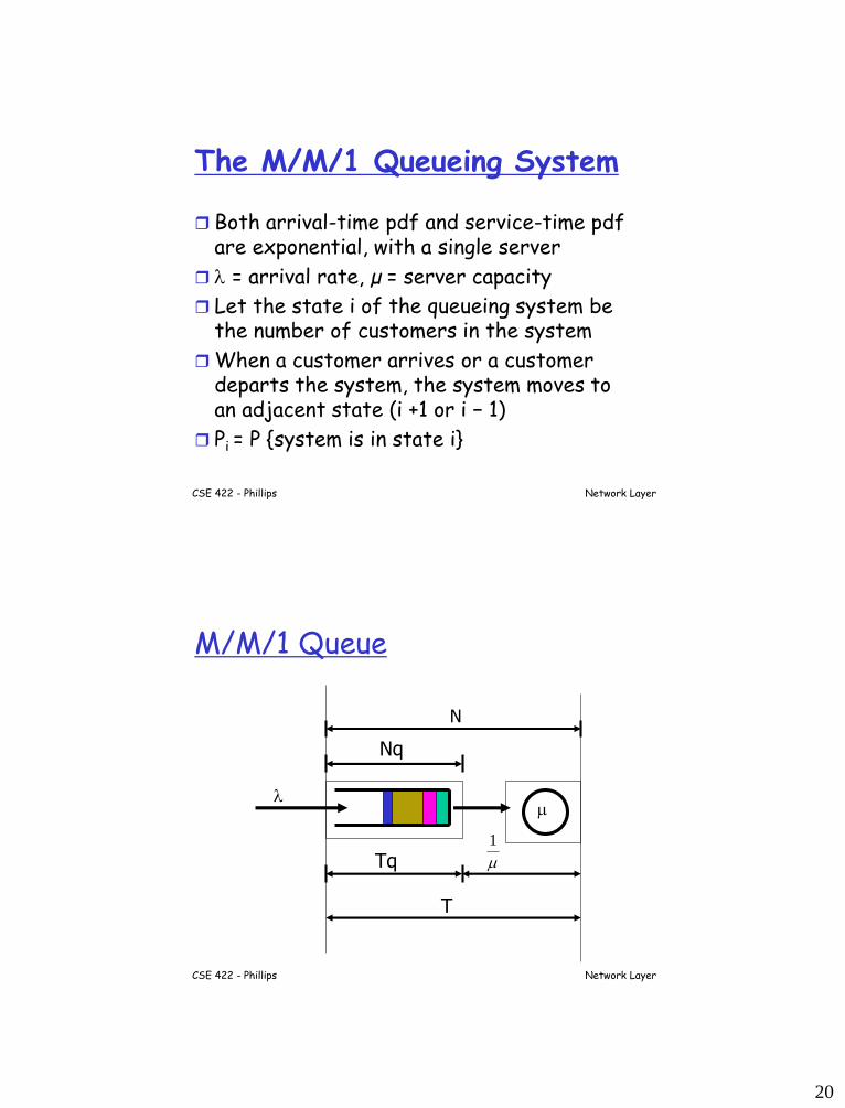
The M/M/1 Queueing System
Both arrival-time pdf and service-time pdf are exponential, with a single server
= arrival rate, µ = server capacity
Let the state i of the queueing system be the number of customers in the system
When a customer arrives or a customer departs the system, the system moves to an adjacent state (i +1 or i − 1)
Pi = P {system is in state i}
Network Layer
CSE 422 - Phillips
M/M/1 Queue
Network Layer
m
m
1
Tq
T
N
Nq
21
CSE 422 - Phillips
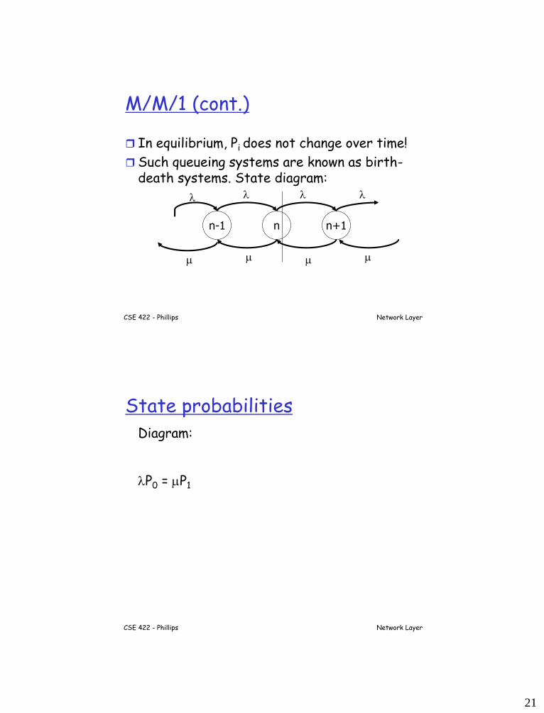
M/M/1 (cont.)
In equilibrium, Pi does not change over time!
Such queueing systems are known as birth-death systems. State diagram:
Network Layer
n+1nn-1
m mm m
CSE 422 - Phillips
State probabilitiesDiagram:
P0 = mP1
Network Layer
22
CSE 422 - Phillips
Solve for P0
Network Layer
CSE 422 - Phillips
M/M/1 at a glance…
What is ρ?
Since and m are constants, Pi alone describes the current state of the system.
Why can we describe the ENTIRE state of the system by a single parameter?
Network Layer
23
CSE 422 - Phillips
Computing N
Network Layer
CSE 422 - Phillips
Computing T
Network Layer
24
CSE 422 - Phillips
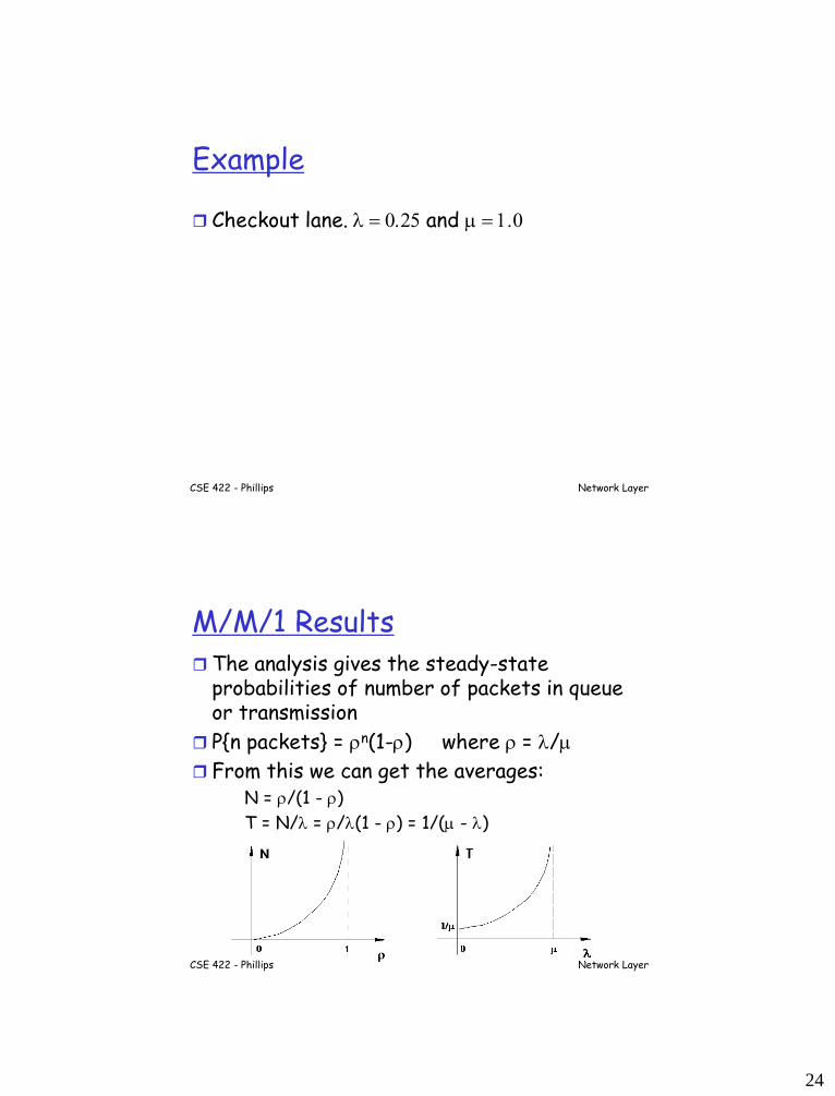
Example
Checkout lane. = 0.25 and m = 1.0
Network Layer
CSE 422 - Phillips
M/M/1 Results The analysis gives the steady-state
probabilities of number of packets in queue or transmission
P{n packets} = rn(1-r) where r = /m
From this we can get the averages: N = r/(1 - r)
T = N/ = r/(1 - r) = 1/(m - )
Network Layer
25
CSE 422 - Phillips
Networking Example
On a network router, measurements show that packets arrive at a mean rate of 125 packets
per second (pps) and
the router takes about 2 milliseconds to forward them.
Assuming an M/M/1 model, What is the probability of buffer overflow if
the router had only 13 buffers?
How many buffers are needed to keep packet loss below one packet per million?
Network Layer
CSE 422 - Phillips
Example (cont.)
Arrival rate λ =
Service rate μ =
Gateway utilization ρ = λ/μ =
Prob. of n packets in gateway =
Mean number of packets in router =
Network Layer
26
CSE 422 - Phillips
Example (cont.)
Probability of buffer overflow:= P(more than 13 packets in gateway)
Network Layer
CSE 422 - Phillips
Example (cont.)
To limit the probability of loss to less than 10-
6:
Network Layer