CSC421 Lecture 2: Linear Models - Department of Computer ...
32
CSC421 Lecture 2: Linear Models Roger Grosse and Jimmy Ba Roger Grosse and Jimmy Ba CSC421 Lecture 2: Linear Models 1 / 30
Transcript of CSC421 Lecture 2: Linear Models - Department of Computer ...

CSC421 Lecture 2: Linear Models
Roger Grosse and Jimmy Ba
Roger Grosse and Jimmy Ba CSC421 Lecture 2: Linear Models 1 / 30

Overview
Some canonical supervised learning problems:
Regression: predict a scalar-valued target (e.g. stock price)Binary classification: predict a binary label (e.g. spam vs. non-spamemail)Multiway classification: predict a discrete label (e.g. object category,from a list)
A simple approach is a linear model, where you decide based on alinear function of the input vector.
This lecture reviews linear models, plus some other fundamentalconcepts (e.g. gradient descent, generalization)
This lecture moves very quickly because it’s all review. But there aredetailed course readings if you need more of a refresher.
Roger Grosse and Jimmy Ba CSC421 Lecture 2: Linear Models 2 / 30

Problem Setup
Want to predict a scalar t as a function of a vector x
Given a dataset of pairs {(x(i), t(i))}Ni=1
The x(i) are called input vectors, and the t(i) are called targets.
Roger Grosse and Jimmy Ba CSC421 Lecture 2: Linear Models 3 / 30

Problem Setup
Model: y is a linear function of x :
y = w>x + b
y is the prediction
w is the weight vector
b is the bias
w and b together are the parameters
Settings of the parameters are called hypothesesRoger Grosse and Jimmy Ba CSC421 Lecture 2: Linear Models 4 / 30

Problem Setup
Loss function: squared error
L(y , t) =1
2(y − t)2
y − t is the residual, and we want to make this small in magnitude
The 12 factor is just to make the calculations convenient.
Cost function: loss function averaged over all training examples
J (w , b) =1
2N
N∑i=1
(y (i) − t(i)
)2=
1
2N
N∑i=1
(w>x(i) + b − t(i)
)2
Roger Grosse and Jimmy Ba CSC421 Lecture 2: Linear Models 5 / 30

Problem Setup
Visualizing the contours of the cost function:
Roger Grosse and Jimmy Ba CSC421 Lecture 2: Linear Models 6 / 30

Vectorization
We can organize all the training examples into a matrix X with onerow per training example, and all the targets into a vector t.
Computing the predictions for the whole dataset:
Xw + b1 =
w>x(1) + b...
w>x(N) + b
=
y (1)
...
y (N)
= y
Roger Grosse and Jimmy Ba CSC421 Lecture 2: Linear Models 7 / 30

Vectorization
Computing the squared error cost across the whole dataset:
y = Xw + b1
J =1
2N‖y − t‖2
In Python:
Roger Grosse and Jimmy Ba CSC421 Lecture 2: Linear Models 8 / 30

Solving the optimization problem
We defined a cost function. This is what we’d like to minimize.
Recall from calculus class: the minimum of a smooth function (if itexists) occurs at a critical point, i.e. point where the partialderivatives are all 0.
Two strategies for optimization:
Direct solution: derive a formula that sets the partial derivatives to 0.This works only in a handful of cases (e.g. linear regression).Iterative methods (e.g. gradient descent): repeatedly apply an updaterule which slightly improves the current solution. This is what we’ll dothroughout the course.
Roger Grosse and Jimmy Ba CSC421 Lecture 2: Linear Models 9 / 30

Direct solution
Partial derivatives: derivatives of a multivariate function with respectto one of its arguments.
∂
∂x1f (x1, x2) = lim
h→0
f (x1 + h, x2)− f (x1, x2)
h
To compute, take the single variable derivatives, pretending the otherarguments are constant.Example: partial derivatives of the prediction y
∂y
∂wj=
∂
∂wj
∑j′
wj′xj′ + b
= xj
∂y
∂b=
∂
∂b
∑j′
wj′xj′ + b
= 1
Roger Grosse and Jimmy Ba CSC421 Lecture 2: Linear Models 10 / 30

Direct solution
Chain rule for derivatives:∂L∂wj
=dLdy
∂y
∂wj
=d
dy
[1
2(y − t)2
]· xj
= (y − t)xj
∂L∂b
= y − t
We will give a more precise statement of the Chain Rule next week.It’s actually pretty complicated.Cost derivatives (average over data points):
∂J∂wj
=1
N
N∑i=1
(y (i) − t(i)) x(i)j
∂J∂b
=1
N
N∑i=1
y (i) − t(i)
Roger Grosse and Jimmy Ba CSC421 Lecture 2: Linear Models 11 / 30
Gradient descent
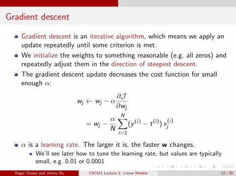
Gradient descent is an iterative algorithm, which means we apply anupdate repeatedly until some criterion is met.
We initialize the weights to something reasonable (e.g. all zeros) andrepeatedly adjust them in the direction of steepest descent.
The gradient descent update decreases the cost function for smallenough α:
wj ← wj − α∂J∂wj
= wj −α
N
N∑i=1
(y (i) − t(i)) x(i)j
α is a learning rate. The larger it is, the faster w changes.We’ll see later how to tune the learning rate, but values are typicallysmall, e.g. 0.01 or 0.0001
Roger Grosse and Jimmy Ba CSC421 Lecture 2: Linear Models 12 / 30

Gradient descent
This gets its name from the gradient:
∇J (w) =∂J∂w
=
∂J∂w1
...∂J∂wD
This is the direction of fastest increase in J .
Update rule in vector form:
w← w − α∇J (w)
= w − α
N
N∑i=1
(y (i) − t(i)) x(i)
Hence, gradient descent updates the weights in the direction offastest decrease.
Roger Grosse and Jimmy Ba CSC421 Lecture 2: Linear Models 13 / 30

Gradient descent
Visualization:http://www.cs.toronto.edu/~guerzhoy/321/lec/W01/linear_
regression.pdf#page=21
Roger Grosse and Jimmy Ba CSC421 Lecture 2: Linear Models 14 / 30

Gradient descent
Why gradient descent, if we can find the optimum directly?
GD can be applied to a much broader set of modelsGD can be easier to implement than direct solutions, especially withautomatic differentiation softwareFor regression in high-dimensional spaces, GD is more efficient thandirect solution (matrix inversion is an O(D3) algorithm).
Roger Grosse and Jimmy Ba CSC421 Lecture 2: Linear Models 15 / 30

Feature maps
We can convert linear models into nonlinear models using featuremaps.
y = w>φ(x)
E.g., if ψ(x) = (1, x , · · · , xD)>, then y is a polynomial in x . Thismodel is known as polynomial regression:
y = w0 + w1x + · · ·+ wDxD
This doesn’t require changing the algorithm — just pretend ψ(x) isthe input vector.
We don’t need an expicit bias term, since it can be absorbed into ψ.
Feature maps let us fit nonlinear models, but it can be hard to choosegood features.
Before deep learning, most of the effort in building a practical machinelearning system was feature engineering.
Roger Grosse and Jimmy Ba CSC421 Lecture 2: Linear Models 16 / 30

Feature maps
y = w0
x
t
M = 0
0 1
−1
0
1
y = w0 + w1x
x
t
M = 1
0 1
−1
0
1
y = w0 + w1x + w2x2 + w3x
3
x
t
M = 3
0 1
−1
0
1
y = w0 + w1x + · · ·+ w9x9
x
t
M = 9
0 1
−1
0
1
-Pattern Recognition and Machine Learning, Christopher Bishop.
Roger Grosse and Jimmy Ba CSC421 Lecture 2: Linear Models 17 / 30
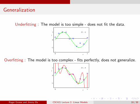
Generalization
Underfitting : The model is too simple - does not fit the data.
x
t
M = 0
0 1
−1
0
1
Overfitting : The model is too complex - fits perfectly, does not generalize.
x
t
M = 9
0 1
−1
0
1
Roger Grosse and Jimmy Ba CSC421 Lecture 2: Linear Models 18 / 30

Generalization
We would like our models to generalize to data they haven’t seenbefore
The degree of the polynomial is an example of a hyperparameter,something we can’t include in the training procedure itself
We can tune hyperparameters using a validation set:
Roger Grosse and Jimmy Ba CSC421 Lecture 2: Linear Models 19 / 30

Classification
Binary linear classification
classification: predict a discrete-valued target
binary: predict a binary target t ∈ {0, 1}Training examples with t = 1 are called positive examples, and trainingexamples with t = 0 are called negative examples. Sorry.
linear: model is a linear function of x, thresholded at zero:
z = wTx + b
output =
{1 if z ≥ 00 if z < 0
Roger Grosse and Jimmy Ba CSC421 Lecture 2: Linear Models 20 / 30

Logistic Regression
We can’t optimize classification accuracy directly with gradientdescent because it’s discontinuous.
Instead, we typically define a continuous surrogate loss function whichis easier to optimize. Logistic regression is a canonical example ofthis, in the context of classification.
The model outputs a continuous value y ∈ [0, 1], which you can thinkof as the probability of the example being positive.
Roger Grosse and Jimmy Ba CSC421 Lecture 2: Linear Models 21 / 30
Logistic Regression
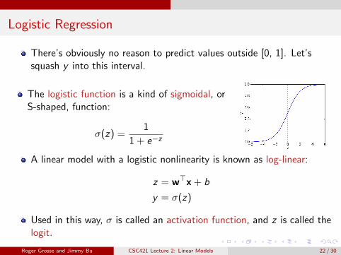
There’s obviously no reason to predict values outside [0, 1]. Let’ssquash y into this interval.
The logistic function is a kind of sigmoidal, orS-shaped, function:
σ(z) =1
1 + e−z
A linear model with a logistic nonlinearity is known as log-linear:
z = w>x + b
y = σ(z)
Used in this way, σ is called an activation function, and z is called thelogit.
Roger Grosse and Jimmy Ba CSC421 Lecture 2: Linear Models 22 / 30

Logistic Regression
Because y ∈ [0, 1], we can interpret it as the estimated probabilitythat t = 1.Being 99% confident of the wrong answer is much worse than being90% confident of the wrong answer. Cross-entropy loss captures thisintuition:
LCE(y , t) =
{− log y if t = 1− log(1− y) if t = 0
= −t log y − (1− t) log(1− y)
Aside: why does it make sense to think of y as a probability? Becausecross-entropy loss is a proper scoring rule, which means the optimal yis the true probability.
Roger Grosse and Jimmy Ba CSC421 Lecture 2: Linear Models 23 / 30

Logistic Regression
Logistic regression combines the logistic activation function withcross-entropy loss.
z = w>x + b
y = σ(z)
=1
1 + e−z
LCE = −t log y − (1− t) log(1− y)
Interestingly, the loss asymptotes to a linear function of the logit z .
Full derivation in the readings.
Roger Grosse and Jimmy Ba CSC421 Lecture 2: Linear Models 24 / 30

Multiclass Classification
What about classification tasks with more than two categories?It is very hard to say what makes a 2 Some examples from an earlier version of the net
Roger Grosse and Jimmy Ba CSC421 Lecture 2: Linear Models 25 / 30

Multiclass Classification
Targets form a discrete set {1, . . . ,K}.It’s often more convenient to represent them as one-hot vectors, or aone-of-K encoding:
t = (0, . . . , 0, 1, 0, . . . , 0)︸ ︷︷ ︸entry k is 1
Roger Grosse and Jimmy Ba CSC421 Lecture 2: Linear Models 26 / 30

Multiclass Classification
Now there are D input dimensions and K output dimensions, so weneed K × D weights, which we arrange as a weight matrix W.
Also, we have a K -dimensional vector b of biases.
Linear predictions:
zk =∑j
wkjxj + bk
Vectorized:z = Wx + b
Roger Grosse and Jimmy Ba CSC421 Lecture 2: Linear Models 27 / 30
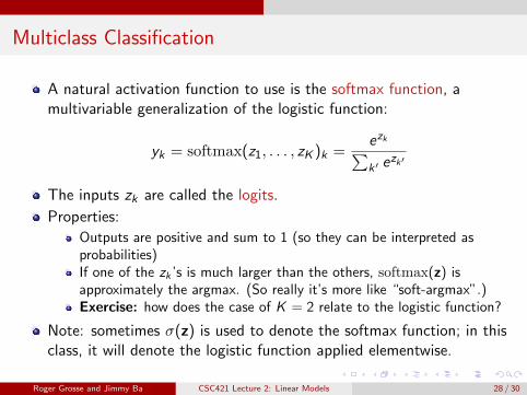
Multiclass Classification
A natural activation function to use is the softmax function, amultivariable generalization of the logistic function:
yk = softmax(z1, . . . , zK )k =ezk∑k ′ ezk′
The inputs zk are called the logits.
Properties:
Outputs are positive and sum to 1 (so they can be interpreted asprobabilities)If one of the zk ’s is much larger than the others, softmax(z) isapproximately the argmax. (So really it’s more like “soft-argmax”.)Exercise: how does the case of K = 2 relate to the logistic function?
Note: sometimes σ(z) is used to denote the softmax function; in thisclass, it will denote the logistic function applied elementwise.
Roger Grosse and Jimmy Ba CSC421 Lecture 2: Linear Models 28 / 30

Multiclass Classification
If a model outputs a vector of class probabilities, we can usecross-entropy as the loss function:
LCE(y, t) = −K∑
k=1
tk log yk
= −t>(log y),
where the log is applied elementwise.
Just like with logistic regression, we typically combine the softmaxand cross-entropy into a softmax-cross-entropy function.
Roger Grosse and Jimmy Ba CSC421 Lecture 2: Linear Models 29 / 30

Multiclass Classification
Softmax regression, also called multiclass logistic regression:
z = Wx + b
y = softmax(z)
LCE = −t>(log y)
It’s possible to show the gradient descent updates have a convenientform:
∂LCE
∂z= y − t
Roger Grosse and Jimmy Ba CSC421 Lecture 2: Linear Models 30 / 30