CSC418 Lecture Notes - yuchenwyc.com

CSC418

Lecture Notes

Yuchen Wang

August 21, 2020

Contents

1 Raster Images 3

2 Ray Casting 42.1 General Ray Casting Algorithm . . . . . . . . . . . . . . . . . . . . . . . . . . . . . . . . . 42.2 Basics . . . . . . . . . . . . . . . . . . . . . . . . . . . . . . . . . . . . . . . . . . . . . . . 42.3 Orthographic/perspective projection . . . . . . . . . . . . . . . . . . . . . . . . . . . . . . 52.4 Ray-Object Intersection . . . . . . . . . . . . . . . . . . . . . . . . . . . . . . . . . . . . . 7

2.4.1 Plane . . . . . . . . . . . . . . . . . . . . . . . . . . . . . . . . . . . . . . . . . . . 72.4.2 Sphere . . . . . . . . . . . . . . . . . . . . . . . . . . . . . . . . . . . . . . . . . . . 72.4.3 Triangle . . . . . . . . . . . . . . . . . . . . . . . . . . . . . . . . . . . . . . . . . . 8

3 Ray Tracing 93.1 General Ray Tracing Algorithm . . . . . . . . . . . . . . . . . . . . . . . . . . . . . . . . . 93.2 Image-order vs Object-order rendering . . . . . . . . . . . . . . . . . . . . . . . . . . . . . 93.3 Two types of lights . . . . . . . . . . . . . . . . . . . . . . . . . . . . . . . . . . . . . . . . 93.4 Shading . . . . . . . . . . . . . . . . . . . . . . . . . . . . . . . . . . . . . . . . . . . . . . 10

3.4.1 Lambertian Shading . . . . . . . . . . . . . . . . . . . . . . . . . . . . . . . . . . . 103.4.2 Blinn-Phong Shading . . . . . . . . . . . . . . . . . . . . . . . . . . . . . . . . . . 103.4.3 Ambient Shading . . . . . . . . . . . . . . . . . . . . . . . . . . . . . . . . . . . . . 113.4.4 Multiple Point Lights . . . . . . . . . . . . . . . . . . . . . . . . . . . . . . . . . . 11

3.5 A Ray-Tracing Program . . . . . . . . . . . . . . . . . . . . . . . . . . . . . . . . . . . . . 113.6 Shadows . . . . . . . . . . . . . . . . . . . . . . . . . . . . . . . . . . . . . . . . . . . . . . 123.7 Ideal Specular Reflection . . . . . . . . . . . . . . . . . . . . . . . . . . . . . . . . . . . . . 12

4 Bounding Volume Hierachy 134.1 Two types of subdivisions . . . . . . . . . . . . . . . . . . . . . . . . . . . . . . . . . . . . 134.2 Bounding Boxes . . . . . . . . . . . . . . . . . . . . . . . . . . . . . . . . . . . . . . . . . 134.3 Axis-Aligned Bounding Boxes Tree (AABB Tree) . . . . . . . . . . . . . . . . . . . . . . . 154.4 Object-Oriented Bounding Box (OOBB) . . . . . . . . . . . . . . . . . . . . . . . . . . . . 174.5 Uniform Spatial Subdivision . . . . . . . . . . . . . . . . . . . . . . . . . . . . . . . . . . . 174.6 Axis-Aligned Binary Space Partitioning (BSP Trees) . . . . . . . . . . . . . . . . . . . . . 17

5 Triangle Meshes 185.1 Mesh Topology . . . . . . . . . . . . . . . . . . . . . . . . . . . . . . . . . . . . . . . . . . 195.2 Indexed Mesh Storage . . . . . . . . . . . . . . . . . . . . . . . . . . . . . . . . . . . . . . 205.3 Triangle Strips and Fans . . . . . . . . . . . . . . . . . . . . . . . . . . . . . . . . . . . . . 215.4 Data Structures for Mesh Connectivity . . . . . . . . . . . . . . . . . . . . . . . . . . . . . 22

1

CONTENTS 2

5.4.1 The Triangle-Neighbor Structure . . . . . . . . . . . . . . . . . . . . . . . . . . . . 225.5 The Winged-Edge Structure . . . . . . . . . . . . . . . . . . . . . . . . . . . . . . . . . . . 245.6 The Half-Edge Structure . . . . . . . . . . . . . . . . . . . . . . . . . . . . . . . . . . . . . 265.7 Different types of normals . . . . . . . . . . . . . . . . . . . . . . . . . . . . . . . . . . . . 275.8 Catmull-Clark subdivision algorithm . . . . . . . . . . . . . . . . . . . . . . . . . . . . . . 28

6 Shader Pipeline 286.1 Rasterization . . . . . . . . . . . . . . . . . . . . . . . . . . . . . . . . . . . . . . . . . . . 31

6.1.1 Triangle Rasterization . . . . . . . . . . . . . . . . . . . . . . . . . . . . . . . . . . 316.2 Operations Before and After Rasterization . . . . . . . . . . . . . . . . . . . . . . . . . . . 31

6.2.1 Vertex-processing stage . . . . . . . . . . . . . . . . . . . . . . . . . . . . . . . . . 316.2.2 Fragment processing stage . . . . . . . . . . . . . . . . . . . . . . . . . . . . . . . . 316.2.3 Blending stage . . . . . . . . . . . . . . . . . . . . . . . . . . . . . . . . . . . . . . 32

7 Kinematics 32

8 Mass-Spring Systems 328.1 Bones . . . . . . . . . . . . . . . . . . . . . . . . . . . . . . . . . . . . . . . . . . . . . . . 328.2 Forward Kinematics . . . . . . . . . . . . . . . . . . . . . . . . . . . . . . . . . . . . . . . 338.3 Keyframe animation . . . . . . . . . . . . . . . . . . . . . . . . . . . . . . . . . . . . . . . 338.4 Inverse Kinematics . . . . . . . . . . . . . . . . . . . . . . . . . . . . . . . . . . . . . . . . 338.5 Projected Gradient Descent . . . . . . . . . . . . . . . . . . . . . . . . . . . . . . . . . . . 348.6 Line Search . . . . . . . . . . . . . . . . . . . . . . . . . . . . . . . . . . . . . . . . . . . . 34

9 Computational Fabrication 34

1 RASTER IMAGES 3

1 Raster Images

1. Raster displays show images as rectangular arrays of pixels.

2. Images should be arrays of floating-point numbers, with either one (for grayscale, or black andwhite images), or three (for RGB color images) 32-bit floating point numbers stored per pixel.

Images as functions Grayscale: I(x, y) : R2 → RRGB: I(x, y) : R2 → R3

Bayer filters A Bayer filter is a color filter array for arranging RGB color filters on a square gridof photosensors. The information is stored as a seemingly 1-channel image, but with an understoodconvention for interpreting each pixel as the red, green or blue intensity value with a fixed pattern.

Demosaic algorithm To demosaic an image, we would like to create a full rgb image without down-sampling the image resolution. For each pixel

1. We’ll use the exact color sample when it’s available;

2. We average available neighbors (in all 8 directions) to fill in missing colors.

Figure 1: a: Bayer filters; bcd: Demosaic algorithm

Image storage on the computer To reduce the storage requirement, most image formats allow forsome kind of compression, either lossless or lossy.

• jpeg: Lossy, compresses image blocks based on thresholds in the human visual system, works wellfor natural images.

• tiff : Losslessly compressed 8- or 16-bit RGB, or hold binary images.

• ppm: Lossless, uncompressed, most often used for 8-bit RGB images. Color intensities are repre-sented as an integer between 0 and 255.

• png: Lossless, with a good set of open source management tools. can store rgba images

In our assignment we use the convention that the red value of pixel in the top-left corner comes first, thenits green value, then its blue value, and then the rgb values of its neighbor to the right and so on acrossthe row of pixels, and then moving to the next row down the columns of rows.

RGB images

2 RAY CASTING 4

HSV images Another useful representation is store the hue, saturation, and value of a color. This”hsv” representation also has 3-channels: typically, the hue or h channel is stored in degrees (i.e., on aperiodic scale) in the range [0◦, 360◦] and the saturation s and value v are given as absolute values in[0, 1].

HSV/RGB conversion Desaturation: Given a factor, for each pixel,

1. Convert RGB values to HSV

2. Let s← (1− factor) ∗ s

3. Convert HSV back to RGB

Hue shifting: Desaturation: Given a shift, for each pixel,

1. Convert RGB values to HSV

2. Let h← (h+ shift) mod 360

3. Convert HSV back to RGB

Grayscale images Take a weighted average of RGB values given higher priority to green:

i = 0.2126r + 0.7152g + 0.0722b (1.1)

Alpha masking It is often useful to store a value α representing how opaque each pixel is.When we store rgb + α image as a 4-channel rgba image. Just like rgb images, rgba images are 3D arraysunrolled into a linear array in memory.

2 Ray Casting

2.1 General Ray Casting Algorithm

for each pixel in the image {

Generate a ray

for each object in the scene {

if (Intersect ray with object){

Set pixel color

}

}

}

2.2 Basics

Notation 2.1. s: the scenee: the camerad: the viewing direction p(t): point along ray

2 RAY CASTING 5

Parametric equation for ray A ray emanating from a point e ∈ R3 in a direction d ∈ R3 can beparameterized by a single number t ∈ [0,∞). Changing the value of t picks a different point along theray. The parametric function for a ray is

p(t) = e + t(s− e) (2.1)

= e + td (2.2)

where p(0) = e and p(1) = s.If 0 < t1 < t2, then p(t1) is closer to the eye than p(t2).Also, if t < 0, then p(t) is “behind” the eye.

Camera space

w = − V iew

||V iew||(2.3)

u = V iew × Up (2.4)

v = w× u (2.5)

2.3 Orthographic/perspective projection

The view that is produced is determined by the choice of projection direction and image plane.

1. Orthographic projection: The image plane is perpendicular to the view direction

2. Oblique projection: The image plane is not perpendicular to the view direction

3. Perspective projection: Project alone lines that pass through a single view point, rather thanalong parallel lines

Orthographic views l and r are the positions of the left and right edges of the image, as measuredfrom e along the u direction; and b and t are the positions of the bottom and top edges of the image, asmeasured from e along the v direction. Usually l < 0 < r and b < 0 < t.To fit an image with nx×ny pixels into a rectangle of size (r− l)× (t− b), the pixels are spaced a distance

2 RAY CASTING 6

(r − l)/nx apart horizontally and (t − b)/ny apart vertically, with a half-pixel space around the edge tocenter the pixel grid within the image rectangle.

u = l + (r − l)(i+ 0.5)/nx (2.6)

v = b+ (t− b)(j + 0.5)/ny (2.7)

where (u, v) are the coordinates of the pixel’s position on the image plane, measured with respect to theorigin e and the basis {u,v}.The procedure for generating orthographic viewing rays is then:

Perspective views The image plane is some distance d (image plane distance) in front of e. Theresulting procedure is

2 RAY CASTING 7

2.4 Ray-Object Intersection

2.4.1 Plane

2.4.2 Sphere

intersect = e + t ∗ d (2.8)

n = (intersect− c).normalized() (2.9)

2 RAY CASTING 8

2.4.3 Triangle

n = [(b− a)× (c− a)].normalized() (2.10)

3 RAY TRACING 9

3 Ray Tracing

3.1 General Ray Tracing Algorithm

3.2 Image-order vs Object-order rendering

Image-order rendering Each pixel is considered in turn, and for each pixel all the objects thatinfluence it are found and the pixel value is computed.Simpler to get working, more flexible in the effects that can be produced, usually takes much moreexecution time to produce a comparable image.

Object-order rendering Each object is considered in turn, and for each object all the pixels that itinfluences are found and updated.

3.3 Two types of lights

Directional Light Direction of light does not depend on the position of the object. Light is very faraway.

3 RAY TRACING 10

Point Light Direction of light depends on position of object relative to light.

3.4 Shading

Notation 3.1. The important variables in light reflection are unit vectorsLight direction l: a unit vector pointing toward the light source;View direction v: a unit vector pointing toward the eye or camera;Surface normal n: a unit vector perpendicular to the surface at the point where reflection is taking place.

3.4.1 Lambertian Shading

An observation by Lambert in the 18th century: the amount of energy from a light source that falls onan area of surface depends on the angle of the surface to the light.

Definition 3.1 (Lambertian shading model). The vector l is computed by subtracting the intersectionpoint of the ray and the surface from the light source position.The pixel color

L = kdI max(0,n · l)

where kd is the diffuse coefficient, or the surface color; and I is the intensity of the light source.

Figure 2: Geometry for Lambertian shading

Remark 3.1. Because n and l are unit vectors, we can use n · l as a convenient shorthand for cos θ. Thisequation applies separately to the three color channels.

Remark 3.2. Lambertian shading is view independent: the color of a surface does not depend on thedirection from which you look. Therefore it does not produce any highlights and leads to a very matte,chalky appearance.

3.4.2 Blinn-Phong Shading

A very simple and widely used model for specular highlights by Phong (1975) and J.F.Blinn (1976).

Idea Produce reflection that is at its brightest when v and l are symmetrically positioned across thesurface normal, which is when mirror reflection would occur; reflection then decreases smoothly as thevectors move away from a mirror configuration.Compare the half vector h with n: if h is near the surface normal, the specular component should bebright and vice versa.

3 RAY TRACING 11

Definition 3.2 (Blinn-Phong shading model).

h =v + l

||v + l||L = kdI max(0,n · l) + ksI max(0,n · h)p

where ks is the specular coefficient, or the specular color of the surface, and p > 1.

3.4.3 Ambient Shading

A heuristic to avoid black shadows is to add a constant component to the shading model, one whosecontribution to the pixel color depends only on the object hit, with no dependence on the surface geometryat all, as if surfaces were illuminated by ambient light that comes equally from everywhere.

Definition 3.3 (simple shading model / Blinn-Phong model with ambient shading).

L = kaIa + kdI max(0,n · l) + ksI max(0,n · h)p

where ka is the surface’s ambient coefficient or “ambient color”, and Ia is the ambient light intensity.

3.4.4 Multiple Point Lights

Property 3.1 (superposition). The effect by more than one light source is simply the sum of the effectsof the light sources individually.

Definition 3.4 (extended simple shading model).

L = kaIa +N∑i=1

[kdIi max(0,n · li) + ksIi max(0,n · hi)p]

where Ii, li and hi are the intensity, direction, and half vector of the i-th light source.

3.5 A Ray-Tracing Program

3 RAY TRACING 12

3.6 Shadows

Recall from 3.4 that light comes from direction l. If we imagine ourselves at a point p on a surface beingshaded, the point is in shadow if we “look” in direction l and see an object. If there are no objects, thenthe light is not blocked.

Remark 3.3. The usual adjustment to avoid the problem of intersecting p with the surface that generatesit is to make the shadow ray check for t ∈ [ε,∞) where ε is some small positive constant.

Remark 3.4. The code above assumes that d and l are not necessarily unit vectors.

3.7 Ideal Specular Reflection

Figure 3: When looking into a perfect mirror, the viewer looking in direction d will see whatever theviewer “below” the surface would see in direction r

r = d− 2(d · n)n

In the real world, a surface may reflect some colors more efficiently than others, so it shifts the colors ofthe objects it reflects (i.e. some energy is lost when the light reflects from the surface).We implement the reflection by a recursive call of raycolor :

color c = c + km * raycolor(p + sr, epsilon, max_t);

4 BOUNDING VOLUME HIERACHY 13

where km is the specular RGB color, p is the intersection of the viewing ray and the surface, s ∈ [ε,max t)for the same reason as we did with shadow rays: we don’t want the reflection ray to hit the object thatgenerates it.To make sure that the recursive call will terminate, we need to add a maximum recursion depth.

4 Bounding Volume Hierachy

4.1 Two types of subdivisions

Object-based subdivision:

• AABB Trees

Spatial subdivision:

• Uniform Spatial Subdivision

• Axis-Aligned Spatial Subdivision

4.2 Bounding Boxes

Definition 4.1. We first consider a 2D ray whose direction vector has positive x and y components. The2D bounding box is defined by two horizontal and two vertical lines:

x = xmin

x = xmax

y = ymin

y = ymax

The points bounded by these lines can be described in interval notation:

(x, y) ∈ [xmin, xmax]× [ymin, ymax]

The intersection test can be phrased in terms of these intervals. First, we compute the ray parameterwhere the ray hits the line x = xmin:

txmin =xmin − xe

xdWe then make similar computations for txmax, tymin, and tymax. The ray hits the box if and only if theintervals [txmin, txmax] and [tymin, tymax] overlap.

Figure 4: The algorithm pseudocode.


Ray-AABB Intersection If max(txmin, tymin, yzmin) < min(txmax, tymax, yzmax), then the ray inter-sects with the box.

Issue 1 The first thing we must address is the case when xd or yd is negative. If xd is negative, thenthe ray will hit xmax before it hits xmin. Thus the code for computing txmin and txmax expands to:

A similar code expansion must be made for the y cases.

Issue 2 A major concern is that horizontal and vertical rays have a zero value for yd and xd, respectively.This will cause divide by zero which may be a problem. We define the rules for divide by zero:For any positive real number a,

+a/0 = +∞

−a/0 = −∞


Figure 5: The new code segment.

4.3 Axis-Aligned Bounding Boxes Tree (AABB Tree)

In our assignment, we will build a binary tree. Conducting queries on the tree will be reminiscent ofsearching for values in a binary search tree.

Basic idea: Place an axis-aligned 3D bounding box around all the objects. Since testing for intersectionwith the box is not free, rays that hit the bounding box will be more expensive to compute than in abrute force search, but rays that miss the box are cheaper. Such bounding boxes can be made hierarchicalby partitioning the set of objects in a box and placing a box around each partition.

Remark 4.1. Each object belongs to one of two sibling nodes, whereas a point in space may be insideboth sibling nodes.

Remark 4.2 (pros and cons). As follows:

• pros: Operations (e.g. growing the bounding box, testing ray intersection or determining closest-point distances with an axis-aligned bounding box) usually reduce to trivial per-component arith-metic. This means the code is simple to write/debug and also inexpensive to evaluate.

• cons: In general, AABBs will not tightly enclose a set of objects.

Ray intersection algorithm The ray intersection algorithm is essentially performing a depth firstsearch.


Distance query algorithm In this algorithm, we are interested in which box in the AABB tree is theclosest to a fixed point.

Remark 4.3 (pros and cons of DFS). As follows:

• pros: The search usually doesn’t have to visit the entire tree because most boxes are not hit by thegiven ray. In this way, many search paths are quickly aborted.

• cons: Every box has some closest point to our query. A naive depth-first search could end upsearching over every box before finding the one with the smallest query.

• BFS is a much better structure since it makes use of a priority queue to explore the current bestlooking path in our tree.

Remark 4.4. Tree construction complexity: O(n log n)Tree traversal complexity: O(n) (worst case)Brute force complexity: O(n)


4.4 Object-Oriented Bounding Box (OOBB)

Find directions of maximum variance using PCA.

4.5 Uniform Spatial Subdivision

In spatial division, each point in space belongs to exactly one node, whereas objects may belong to manynodes.The scene is partitioned into axis-aligned boxes. These boxes are all the same size, although they are notnecessarily cubes. The ray traverses these boxes. When an object is hit, the traversal ends.

This traversal is done in an increment fashion. We need to find the index (i, j) of the first cell hit by theray e + td. Then we need to traverse the cells in an appropriate order.

4.6 Axis-Aligned Binary Space Partitioning (BSP Trees)

We can also partition space in a hierarchical data structure such as a binary space partitioning tree (BSPtree). It’s common to use axis-aligned cutting planes for ray intersection.A node in this structure contains a single cutting plane and a left and right subtree. Each subtree containsall the objects on one side of the cutting plane. Objects that pass through the plane are stored in bothsubtrees. If we assume the cutting plane is parallel to the yz plane at x = D, then the node class is:

The intersection code can then be called recursively in an object-oriented style. The code considersthe four cases:

5 TRIANGLE MESHES 18

The origin of these rays is a point at parameter t0:

p = a + t0b

The four cases are:

1. The ray only interacts with the left subtree, and we need not test it for intersection with the cuttingplane. It occurs for xp < D and xb < 0.

2. The ray is tested against the left subtree, and if there are no hits, it is then tested against theright subtree. We need to find the ray parameter at x = D, so we can make sure we only test forintersections within the subtree. This case occurs for xp < D and xb > 0.

3. This case is analogous to case 1 and occurs for xp > D and xb > 0.

4. This case is analogous to case 2 and occurs for xp > D and xb < 0.

The resulting traversal code handling these cases in order is:

5 Triangle Meshes

Motivation

• Mesh is a basic computer graphics data structure.

• Most real-world models are composed of complexes of triangles with shared vertices. These areusually known as triangle meshes, and handling them efficiently is crucial to the performance ofmany graphics programs.


• We’d like to minimize the amount of storage consumed.

• Besides basic operations (storing & drawing), other operations such as subdivision, mesh editing andmesh compression, efficient access to adjacency information is crucial.

5.1 Mesh Topology

Property 5.1 (Manifold meshes). The topology of a mesh is a manifold surface: A surface in which asmall neighborhood around any point could be smoothed out into a bit of flat surface.

Verifying the property Prevent crashes or infinite loops by checking:

1. Every edge is shared by exactly two triangles. (as in figure 12.1)

2. Every vertex has a single, complete loop of triangles around it. (as in figure 12.2)

Property 5.2 (Manifold with boundary meshes). Sometimes it’s necessary to allow meshes to haveboundaries. Such meshes are not manifolds. However, we can relax the requirements of a manifold meshto those for a manifold with boundary without causing problems for most mesh processing algorithms.The relaxed conditions are:

1. Every edge is used by either one or two triangles.

2. Every vertex connects to a single edge-connected set of triangles.


Figure 12.3 illustrates these conditions.

Property 5.3 (orientation). For a single triangle, we define orientation based on the order in whichthe vertices are listed: the front is the side from which the triangle’s three vertices are arranged incounterclockwise order.A connected mesh is consistently oriented if its triangles all agree on which side is the front.

5.2 Indexed Mesh Storage

Definition 5.1 (Separate triangles). Store each triangle as an independent entity.

Triangle {

vector3 vertexPosition[3]

}

Definition 5.2 (Indexed Shared-vertex mesh). This data structure has triangles which point to verticeswhich contain the vertex data:

Triangle {

Vertex v[3]

}

Vertex {

vector3 position

}

In implementation, the vertices and triangles are normally stored in arrays:

IndexedMesh{

int tInd[nt][3]

vector3 verts[nv]

}


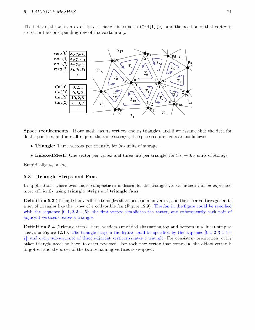
The index of the kth vertex of the ith triangle is found in tInd[i][k], and the position of that vertex isstored in the corresponding row of the verts arary.

Space requirements If our mesh has nv vertices and nt triangles, and if we assume that the data forfloats, pointers, and ints all require the same storage, the space requirements are as follows:

• Triangle: Three vectors per triangle, for 9nt units of storage;

• IndexedMesh: One vector per vertex and three ints per triangle, for 3nv + 3nt units of storage.

Empirically, nt ≈ 2nv.

5.3 Triangle Strips and Fans

In applications where even more compactness is desirable, the triangle vertex indices can be expressedmore efficiently using triangle strips and triangle fans.

Definition 5.3 (Triangle fan). All the triangles share one common vertex, and the other vertices generatea set of triangles like the vanes of a collapsible fan (Figure 12.9). The fan in the figure could be specifiedwith the sequence [0, 1, 2, 3, 4, 5]: the first vertex establishes the center, and subsequently each pair ofadjacent vertices creates a triangle.

Definition 5.4 (Triangle strip). Here, vertices are added alternating top and bottom in a linear strip asshown in Figure 12.10. The triangle strip in the figure could be specified by the sequence [0 1 2 3 4 5 67], and every subsequence of three adjacent vertices creates a triangle. For consistent orientation, everyother triangle needs to have its order reversed. For each new vertex that comes in, the oldest vertex isforgotten and the order of the two remaining vertices is swapped.


In both strips and fans, n+ 2 vertices suffice to describe n triangles.

5.4 Data Structures for Mesh Connectivity

5.4.1 The Triangle-Neighbor Structure

Augmenting the basic shared-vertex mesh with pointers from the triangles to the three neighboringtriangles, and a pointer from each vertex to one of the adjacent triangles (it doesn’t matter which one)

Triangle {

Triangle nbr[3];


Vertex v[3];

}

Vertex {

// ... per-vertex data ...

Triangle t; // any adjacent tri

}

In the array Triangle.nbr, the kth entry points to the neighboring triangle that shares vertices k andk + 1.Implementation:

Mesh{

vector3 verts[nv] // per-vertex data

int tInd[nt][3]; // vertex indices

int tNbr[nt][3]; // indices of neighbor triangles

int vTri[nv]; // index of any adjacent triangle

}

The idea is to move from triangle to triangle, visiting only the triangles adjacent to the relevant vertex.If triangle t has vertex v as its kth vertex, then the triangle t.nbr[k] is the next triangle around v in theclockwise direction. This observation leads to the following algorithm to traverse all the triangles adjacentto a given vertex:

TrianglesOfVertex(v) { t = v.t

do {

find i such that (t.v[i] == v) t = t.nbr[i]

} while (t != v.t) }


A small refinement to let us find the previous triangle:

Triangle {

Edge nbr[3];

Vertex v[3];

}

Edge { // the i-th edge of triangle t Triangle t;

int i; // in {0,1,2}

}

Vertex {


Edge e; // any edge leaving vertex

}

TrianglesOfVertex(v) {

{t, i} = v.e;

do {

{t, i} = t.nbr[i];

i = (i+1) mod 3;

} while (t != v.e.t);

}

5.5 The Winged-Edge Structure

In a winged-edge mesh, each edge stores pointers to the two vertices it connects (the head and tail vertices),the two faces it is part of (the left and right faces), and, most importantly, the next and previous edges inthe counterclock- wise traversal of its left and right faces (Figure 12.16). Each vertex and face also storesa pointer to a single, arbitrary edge that connects to it:


Edge {

Edge lprev, lnext, rprev, rnext;

Vertex head, tail;

Face left, right;

}

Face {

// ... per-face data ...

Edge e; // any adjacent edge

}

Vertex {

// ... per-vertex data ... Edge e; // any incident edge

}

The search algorithm:


5.6 The Half-Edge Structure

The winged-edge structure is quite elegant, but it has one remaining awkward- ness—the need to con-stantly check which way the edge is oriented before moving to the next edge.Solution: Store data for each half-edge. There is one half-edge for each of the two triangles that sharean edge, and the two half-edges are oriented oppositely, each oriented consistently with its own triangle.The data normally stored in an edge is split between the two half-edges. Each half-edge points to theface on its side of the edge and to the vertex at its head, and each contains the edge pointers for its face.It also points to its neighbor on the other side of the edge, from which the other half of the informationcan be found.

HEdge {

HEdge pair, next;

Vertex v;

Face f;

}

Face {

// ... per-face data ...

HEdge h; // any h-edge of this face

}

Vertex {


HEdge h; // any h-edge pointing toward this vertex

}


The search algorithm:

EdgesOfVertex(v) {

h = v.h;

do {

h = h.pair.next;

} while (h != v.h);

}

EdgesOfFace(f) {

h = f.h;

do {

h = h.next;

} while (h != f.h);

}

The vertex traversal here is clockwise, which is necessary because of omitting the prev pointer fromthe structure.Because half-edges are generally allocated in pairs (at least in a mesh with no boundaries), many im-plementations can do away with the pair pointers. For instance, in an implementation based on arrayindexing (such as shown in Figure 12.18), the array can be arranged so that an even-numbered edge ialways pairs with edge i+ 1 and an odd-numbered edge j always pairs with edge j − 1.In addition to the simple traversal algorithms shown in this chapter, all three of these mesh topologystructures can support ”mesh surgery” operations of various sorts, such as splitting or collapsing vertices,swapping edges, adding or removing triangles, etc.

5.7 Different types of normals

Per-Face Normals The surface will have a faceted appearance. This appearance is mathematicallycorrect, but not necessarily desired if we wish to display a smooth looking surface.

Per-Vertex Normals Corners of triangles located at the same vertex should share the same normalvector. Smooth appearance. A common way to define per-vertex normals is to take a area-weighted

6 SHADER PIPELINE 28

average of normals from incident faces:

nv =

∑f∈N(v) afnf

||∑

f∈N(v) afnf ||(5.1)

where N(v) is the set of faces neighboring the v-th vertex, af is the area of face f , and nf is the normalvector of face f .

Per-Corner Normals For surfaces with a mixture of smooth-looking parts and creases, it is useful todefine normals independently for each triangle corner (as opposed to each mesh vertex). For each corner,we’ll again compute an area-weighted average of normals triangles incident on the shared vertex at thiscorner, but we’ll ignore triangle’s whose normal is too different from the corner’s face’s normal:

nf,c =

∑g∈N(v)|ng ·nf>ε

agng

||∑

g∈N(v)|ng ·nf>εagng||

(5.2)

where ε is the minimum dot product between two face normals before we declare there is a crease betweenthem.

5.8 Catmull-Clark subdivision algorithm

Subdivision Surfaces A Recursive refinement of polygonal mesh that results in smooth “limit surface”.

Catmull-Clark subdivision algorithm The first and still popular subdivision scheme.

1. Set the face point for each facet to be the average of its vertices.

2. Add edge points - average of two neighboring face points and edge end points.

3. Add edges between face points and edge points.

4. Move each original vertex according to new position given by

F + 2R+ (n− 3)P

n

where F is average of all n created face points adjacent to P and R is average of all original edgemidpoints touching P .

5. Connect up original points to make facets

6. RepeatIf texture co-ordinates is onthe test, lookup textbookp2496 Shader Pipeline

Definition 6.1 (rasterization). The process of finding all the pixels in an image that are occupied by ageometric primitive is called rasterization.

Definition 6.2 (graphics pipeline). The sequence of operations that is required, starting with objectsand ending by updating pixels in the image, is known as the graphics pipeline.


Tessellation control shader Determines how to subdivide each input patch. The subdivision isdetermined independently for each triangle and not called recursively.Unlike the vertex or fragment shader, the tessellation control shader has access to attribute informationat all of the vertices of a triangle.

Tessellation evaluation shader Takes the result of the tessellation that the “tessellation controlshader” has specified. This shader is called once for every vertex output during tessellation. It hasaccess to the attribute information of the original corners and a special variable gl TessCoord containingthe barycentric coordinates of the current vertex. Using this information, it is possible to interpolateinformation stored at the original corners onto the current vertex (e.g. the 3D position).

Definition 6.3 (Bump map). A bump map is a mapping from a surface point to a displacement alongthe normal direction. Each point p ∈ R3 on the surface is moved to a new position p ∈ R3:

p(p) := p + h(p)n(p) (6.1)

where h : R3 → R is the bump height amount function (could be negative) and n(p) : R3 → R3 is themathematically correct normal at p.

Remark 6.1. The idea is that a bump map is a height field: a function that give the local height of thedetailed surface above the smooth surface.


Definition 6.4 (Normal map). A normal map is a mapping from a surface point to a unit normalvector.To create a consistent and believable looking normal map, we can first generate a plausible bump map.If our bump height h is a smooth function over the surface, we can compute the perceived normal vectorn by taking a small finite difference of the 3D position:

n =∂p

∂T× ∂p

∂B≈(

p(p + εT )− p(p)

ε

)×(

p(p + εB)− p(p)

ε

)(6.2)

where T,B ∈ R3 are orthogonal tangent and bi-tangent vectors in the tangent plane at p and ε is a smallnumber (e.g. 0.0001).We’ll make sure that this approximate perceived normal is unit length by dividing by its length:

n← n

||n||(6.3)

Remark 6.2. Normal mapping is useful in computer graphics because we can drape the appearance ofa complex surface on top a low resolution and simple one.

Remark 6.3. Normal mapping makes the shading normal depend on values read from a texture map.

Remark 6.4. It does not change the surface at all, just a shadowing trick that create the illusion ofdepth detail on the surface of a model.

A type of gradient noise used to produce natural appearing textures.

1. Grid definition: Define an n-dimensional grid where each point has a random n-dimensional unit-length gradient vector.

2. Dot product: An n-dimensional candidate point can be viewed as falling into an n-dimensional gridcell. Fetch the 2n closest gradient values, located at the 2n corners of the grid cell. Then for eachgradient value, compute a distance vector from each corner node to the candidate point. Thencompute the dot product between each pair of gradient vector and distance vector. This functionhas a value of 0 at the node and a gradient equal to the precomputed node gradient.

3. Interpolation: Performed using a function that has zero first derivative at the 2n grid nodes.

If n = 1, an example of a function that interpolates between value a0 at grid node 0 and value a1 at gridnode 1 is

f(x) = a0 + smoothstep(x) · (a1 − a0) (6.4)

for 0 ≤ x ≤ 1, where

smoothstep(x) =

0 x ≤ 0

3x2 − 2x3 0 ≤ x ≤ 1

1 x ≥ 1

(6.5)

Definition 6.5. Tangent and bitangent vector Let s(x, y, z) and t(x, y, z) be differentiable scalar functionsdefined at all points on a surface S. In computer graphics, the functions s and t often represent texturecoordinates for a 3-dimensional polygonal model. In this context, the tangent vector T (px, py, pz) isspecifically defined to be the unit vector lying in the tangent plane for which

gradT t(px, py, pz) = 0, gradT s(px, py, pz) > 0 (6.6)

The bitangent vector B(px, py, pz) is defined to be the unit vector lying in the tangent plane for which

gradT s(px, py, pz) = 0, gradT t(px, py, pz) > 0 (6.7)


Remark 6.5. The vectors T and B are not necessarily orthogonal and may not exist for poorly condi-tioned functions s and t.

6.1 Rasterization

For each primitive that comes in, the rasterizer has two jobs:

1. It enumerates the pixels that are covered by the primitive.

2. It interpolates values, called attributes, across the primitive.

The output is called fragments, one for each pixel covered by the primitive. Each fragment “lives” at aparticular pixel and carries its own set of attribute values.

6.1.1 Triangle Rasterization

Definition 6.6 (Gouraud interpolation). If the vertices have colors c0, c1 and c2, the color at a point inthe triangle with barycentric coordinates (α, β, γ) is

c = αc0 + βc1 + γc2 (6.8)

We are usually rasterizing triangles that share vertices and edges. To draw them with no holes, we canuse the midpoint algorithm to draw the outline of each triangle and then fill in the interior pixels.Pixels are drawn iff their centers are inside the triangle, i.e., the barycentric coordinates of the pixel centerare all in the interval (0, 1).

Figure 6: Algorithm for triangle rasterization.

6.2 Operations Before and After Rasterization

6.2.1 Vertex-processing stage

1. Incoming vertices are transformed by the modeling, viewing, and projection transformations, map-ping them from their original coordinates into screen space.

2. Other information, such as colors, surface normals, or texture coordinates, is transformed as needed.

6.2.2 Fragment processing stage

1.

7 KINEMATICS 32

6.2.3 Blending stage

Combines the fragments generated by the primitives that overlapped each pixel to compute the finalcolor. The most common blending approach is to choose the color of the fragment with the smallestdepth (closest to the eye).

Using a z-buffer for hidden surfaces At each pixel, we keep track of the distance to the closest surfacethat has been drawn so far, and we throw away fragments that are farther away than that distance.The closest distance is stored by allocating an extra value for each pixel, in addition to the rgb values,which is known as the depth, or z-value. The z-buffer is the name for the grid of depth values.

Remark 6.6. Of course there can be ties in the depth test, in which case the order may well matter.

7 Kinematics

Study of motion without consideration of what causes that motion.

8 Mass-Spring Systems

8.1 Bones

Definition 8.1 (skeleton). A skeleton is a tree of rigid bones. Each bone in the skeleton is a UI widgetfor visualizing and controlling a 3D rigid transformation. A common visualization of 3D bone in computergraphics is a long, pointed pyramid shape.

Definition 8.2 (Canonical bones). The “canonical bone” of length l lies along the x-axis with its “tail”at the origin (0, 0, 0), its “tip” at (l, 0, 0).Twisting is rotating about the x-axis in the canonical frame.Bending is rotating about the z-axis in the canonical frame.

Remark 8.1. Composing a twist, bend and another twist spans all possible 3D rotations. We call thethree angles composed into a rotation this way, Euler angles.

Definition 8.3 (Rest bones). For each bone, there is a rigid transformation that places its tail and tipto the desired positions in the model.

T =(Rt)∈ R3×4 (8.1)

where T = transformation, R = rotation and t = translation. We use the convention that the “canonicaltail” (the origin (0, 0, 0)) is mapped to the “rest tail” inside the model. This means that the translationpart of the matrix T is simply the rest tail position s ∈ R3:

s = T

0001

= R

000

+ t1 = t (8.2)

The bone’s rotation is chosen so that the “canonical tip” maps to the “rest tip” d ∈ R3:

d = T

l001

= R

l00

+ t1 = t (8.3)

Typically the “rest tail” of a bone is coincident with the “rest tip” of its parent (if it exists)

dp = s (8.4)

8 MASS-SPRING SYSTEMS 33

Remark 8.2. The pose of each bone will be measured relative to the “rest bone”.

Definition 8.4 (Pose bones). In general, each rest bone undergoes a rigid transformation T ∈ R3×4,composed of a rotation R ∈ R3×4 and a translation t ∈ R3, mapping each of its rest points x ∈ R3 to itscorresponding posed position x ∈ R3:

x = T x (8.5)

Remark 8.3. In particular, we would like each bone to rotate about its parent’s tip, but this position isdetermined by the parent’s pose transformation Tp, which in turn should rotate about the grandparent’stip and so on.

8.2 Forward Kinematics

For each bone i in a skeleton, we aggregate relative rotations Ri ∈ R3×3 between a bone i and its parentbone pi in the skeletal tree.For each bone:

1. First undo the map from canonical to rest (inverting Ti);

2. Then rotate by the relative rotation Ri;

3. Then map back to rest (via Ti);

4. Continue up the tree recursively applying the parent’s relative transformation.

Ti = Tpi(Ti)

(8.6)

Definition 8.5 (Linear Blend Skinning). Skinning is the process of defining how bones are attached tothe meshes. In linear blend skinning, each vertex i of the mesh is assigned a weight wi,j for each bone jcorresponding to how much it is “attached” to that bone on a scale of 0% to 100%:

vi =

m∑j=1

wi,jTj

(vi1

)(8.7)

8.3 Keyframe animation

To create a long animation, specifying three Euler angles for every bone for every frame manually wouldbe too difficult. The standard way to determine the relative bone transformations for each frame is tointerpolate values specified at a small number of ”key” times during the animation.

Definition 8.6 (Catmull-Rom interpolation). θ = c(t) is a curve in the pose space. A cubic Hermitespline is a spline where each piece is a third-degree polynomial specified by its values and first derivatives.

incomplete

8.4 Inverse KinematicsA6

https://github.com/psarahdactyl/computer-graphics-kinematics

9 COMPUTATIONAL FABRICATION 34

8.5 Projected Gradient DescentA6

8.6 Line SearchA6

9 Computational Fabrication



CSC418 Lecture Notes - yuchenwyc.com

Documents

Transcript of CSC418 Lecture Notes - yuchenwyc.com