Predictive Maintenance

June Kwon

[ Please Note ]

▪ I used MATLAB to implement the machine learning algorithms.

▪ You can download the codes for this project if you are interested in checking it out. (Link Below)

▪ (The download link server is from my school – Drexel University. Thus, it is a safe link.)

predictiveCode.zip

Thank you very much,

June Kwon

Introduction• Sooner or later, all machines run to failure, but with a wide

range of consequences…

• An unexpected malfunction in a power plant has the potential to leave thousands of people in total darkness for hours and cause a multimillion-dollar loss.

• The average cost of unplanned downtime in energy, manufacturing, transportation, and other industries runs at $250,000 per hour or $2 million per working day. [1]

• To prevent expensive outages from happening and alleviate the damage caused by breakdowns, companies need an efficient maintenance policy.

• Among many available strategies and resources, one of the most advanced approaches is – “Predictive Maintenance”.

Image Source: Google

• As shown right, in the past, people used to perform

the reactive maintenance, meaning that the actions

were taken when the equipment was already down.

• While the reactive maintenance requires no initial

maintenance costs, it turns out to be very expensive in terms

of the repair cost.

• Then people looked at the preventive maintenance,

where people performed regular equipment

inspections to mitigate the degradations and reduce

the likelihood of failures.

• However, it still came with a medium range maintenance &

repair cost, causing the companies to take the risk of

performing too much maintenance or not enough.

IntroductionImage Source: Altexsoft [1]

Introduction• Predictive Maintenance solves these issues.

• Predictive Maintenance is a type of condition-

based maintenance where maintenance is only

scheduled when specific conditions are met

and before the equipment breaks down.

• Driven by automation, machine learning, and real-

time data, we can monitor the trends of the machine

performance, and once unhealthy trends are

identified, we will estimate when the maintenance

should be performed to replace/repair the damaged

parts to avoid more costly failures.

• It promises more cost savings over routine or

time-based preventive maintenance.

Image Source: Google

Data Preparation• Let’s take a look at the data I obtained.

• AI4I 2020 Predictive Maintenance Dataset – UCI Machine Learning Repository

• 120 Units – each unit containing 75-85 observations.

• Thus, in total, this dataset contains 10,000 observations.

Features Targets

If at least one of these four failure modes is set to true, the process fails, and the “Machine Failure” label is set to true.

UDI Product ID Type

Air

temperat

ure [K]

Process

Temperat

ure [K]

Rotational

Speed

[rpm]

Torque

[Nm]

Tool

Wear

Time

[min]

Machine

Failure

Tool Wear

Failure

(TWF)

Heat

Dissipatio

n Failure

(HDF)

Power

Failure

(PWF)

Overstrain

Failure

(OSF)

1 M14860 M 298.1 308.6 1551 42.8 0 0 0 0 0 0

2 L47181 L 298.2 308.7 1408 46.3 3 0 0 0 0 0

443 L47622 L 297.4 308.5 1399 61.5 61 1 0 0 1 0

1997 M16856 L 298.4 308 1416 38.2 198 1 1 0 0 0

2126 L49305 L 299.3 308.9 1258 69.4 119 1 0 0 1 0

2380 H31793 M 299.1 308.2 1450 46.1 112 0 0 0 0 0

4872 L52051 L 303.7 312.4 1513 40.1 135 0 0 0 0 0

• In order to have deeper understanding of the data, the distribution of each data point was visualized as shown in the picture right.

• Air Temperature and Process Temperature show quite consistent data distribution over the wear time. Most of the data in Air Temperature and Process Temperature reside at the temperature of 300 Kelvin and 310 Kelvin, respectively.

• For Rotational Speed and Torque data, it can be noted that the most of data reside at the speed of 1500 RPM and at the Torque value of 40 Nm.

• By visualizing the data, I can understand the data more deeply. For example, it can be expected that any values deviated from the accumulated region may be classified as “Abnormal”.

Data Analysis

• Moreover, the PCA has been performed

for deeper understanding of the data as

shown in the picture right. It represents

the data plotted over the 1st principal

component as x-axis and 2nd principal

component as y-axis.

• From the figure, it can be noted that most

of the data reside at from 1400 to 1600 on

the 1st principal component (x-axis), and

from 0 to 200 on the 2nd principal

component (y-axis)

• It can then be expected that values

deviated from this accumulated region can

be classified as "Abnormal".

Data Analysis

Approach

1. Predict the remaining useful life of an equipment (RUL Analysis)

• Enables monitoring for health diagnostic, and plan maintenance schedules.

2. Predict the possible root cause of the failure.

• Recommends the right set of maintenance actions to fix a failure

• Now we’ve looked at data and its distribution, let’s talk about the types of

approaches to implement the predictive maintenance.

• There are two types of analysis we can perform as shown below.

“Let’s look at each type of analysis.”

Image Source: Microsoft [2]

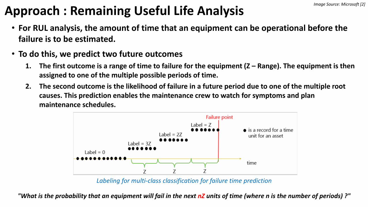
Approach : Remaining Useful Life Analysis• For RUL analysis, the amount of time that an equipment can be operational before the

failure is to be estimated.

• To do this, we predict two future outcomes1. The first outcome is a range of time to failure for the equipment (Z – Range). The equipment is then

assigned to one of the multiple possible periods of time.

2. The second outcome is the likelihood of failure in a future period due to one of the multiple root causes. This prediction enables the maintenance crew to watch for symptoms and plan maintenance schedules.

Labeling for multi-class classification for failure time prediction

"What is the probability that an equipment will fail in the next nZ units of time (where n is the number of periods) ?"

Image Source: Microsoft [2]

• Let’s take a look at the example.

• Looking at the entire timeline of the engine life, we align the failure point on same timeline, and from there, the specific user-defined range of time that is closest to the failure point will be assigned a class “Urgent”.

• Then, next closest range of time will be assigned a class “Medium”, and the most distant range of time from failure point will be assigned a class “Long” which means it still has long remaining useful life. (it does not require maintenance as of now.)

• Using this modeling techniques, it is possible to properly construct the specific classes on the data.

Modeling Techniques

(Specific Label Construction Method)

Approach : Remaining Useful Life Analysis

Failure Point

Image Source: MathWorks [4]

• For Possible Root Cause Analysis, the most likely root cause of a given failure is to be estimated.• This outcome recommends the right set of maintenance actions to fix a failure. A list

of root causes can be ranked to recommend repairs which can help technicians prioritize their repair actions after a failure.

Labeling for multi-class classification for root cause prediction

Approach : Possible Root Cause Analysis

"What is the probability that an equipment will fail in the next X units of time due to root cause/problem Pi?"

(where i is the number of possible root causes).

Image Source: Microsoft [2]

• Finally, let’s apply various machine learning techniques to the given dataset to train the model.

• I will consider below four classifiers to train my models…

1. Logistic Regression (with Cross Validation)

2. Naïve Bayes

3. Decision Tree

4. K-Nearest Neighbors

(All as a multiclassification problem…)

• Then the performance of each classifier will be evaluated to choose the best classifier for the given dataset…

• Consider/compare their accuracies, precisions, recalls, f-measures, confusion matrix, etc.

• Then I would like to use above two types of predictive maintenance scenarios to predict the time to failure and the possible root cause of the failure.

ResultImage Source: Google

Results : 1. Remaining Useful Life• Remaining Useful Life Analysis has been performed by modelling the

failure time into multiple time ranges as follows:

• Assign Class Y = 4 (Urgent) for 90 min before failure

• Assign Class Y = 3 (Short) for 144 min before failure

• Assign Class Y = 2 (Medium) for 198 min before failure

• Assign Class Y = 1 (Long) for greater than 198 min before failure.

1st

Feature

2nd

Feature

3rd

Feature

4th

Feature

5th

FeatureY = nZ

6th

Feature

UDI Product ID Type

Air

temperat

ure [K]

Process

Temperat

ure [K]

Rotational

Speed

[rpm]

Torque

[Nm]

Tool

Wear

Time

[min]

Machine

Failure

Tool

Wear

Failure

(TWF)

Heat

Dissipation

Failure (HDF)

Power

Failure

(PWF)

Overstrain

Failure

(OSF)

1 M14860 M 298.1 308.6 1551 42.8 0 0 0 0 0 0

2 L47181 L 298.2 308.7 1408 46.3 3 0 0 0 0 0

443 L47622 L 297.4 308.5 1399 61.5 61 1 0 0 1 0

1997 M16856 L 298.4 308 1416 38.2 198 1 1 0 0 0

2126 L49305 L 299.3 308.9 1258 69.4 119 1 0 0 1 0

2380 H31793 M 299.1 308.2 1450 46.1 112 0 0 0 0 0

4872 L52051 L 303.7 312.4 1513 40.1 135 0 0 0 0 0

90144198

Features and Targets were selected as shown here for RUL analysis.

Image Source: MathWorks [4]

Results : 1. Remaining Useful Life

• First, Naïve Bayes & Decision Tree Classifiers were used to train the model, and above two pictures show the resulting confusion matrix.

• For Naive Bayes Model, an accuracy of 0.994 was achieved.

• For Decision Tree Model, an accuracy of 0.501 was achieved.

• It is evident that the decision tree model did not perform as good as the naive bayes model. It also can be noted that the decision tree model is unable to distinguish the difference between "Long (Y = 1)" and "Medium (Y = 2)“ classes (green box). It seems that the decision tree model mis-classified the medium class to be the long class.

• I suspect that the possible source of this error is due the highly biased distribution in the data.

• As the unit approaches the failure point, deviation of malfunctioning units (such as Urgent and Short classes) are clearly identifiable from the accumulated region in the dataset.

• However, for the normal operation such as Long and Medium classes, it can become highly unpredictable for the model to distinguish the difference between the two normal operation classes because both Long and Medium classes reside in accumulated regions (green box).

• Thus, this is the possible reason why decision tree did not work well for the given dataset. Thus, the possible solution is to install more sensors that can induce/identify the difference between the Long and the Medium class.

Results : 1. Remaining Useful Life

Results : 1. Remaining Useful Life

• For K-Nearest Neighbor classifier, the algorithm was run with varying K from 1 to 1500 in the increment of 100.

• At K = 601, the highest accuracy of 0.867 was achieved.

• The model is achieving around 86% to 88% which is good, but not as high as the Naïve Bayes classifier.

Algorithm Accuracy

Naïve Bayes 0.994

Decision Tree 0.501

K-Nearest Neighbor 0.867

Logistic Regression 0.992

Results : 1. Remaining Useful Life

Prediction Performance on Remaining Useful Life Analysis

• For Logistic Regression classifier, the algorithm was run with varying learning rate.

• At the learning rate of 0.1, the highest accuracy of 0.992 was achieved.

• Therefore, considering all four algorithms, it has been determined that Naïve Bayes Classifier performed the best for Remaining Useful Life Analysis.

Results : 2. Possible Root Cause• Possible Root Cause Analysis has been performed

by modelling each failure mode as follows:

• Assign Class Y = 1 for No Failure (Normal)

• Assign Class Y = 2 for Tool Wear Failure (TWF)

• Assign Class Y = 3 for Heat Dissipation Failure (HDF)

• Assign Class Y = 4 for Power Failure (PWF)

• Assign Class Y = 5 for Overstrain Failure (OSF)

• However, there was highly biased distribution in data.

• Out of 10,000 observations,

• Nearly 9670 observations are Class Y = 1

• Nearly 40 observations are Class Y = 2

• Nearly 110 observations are Class Y = 3

• Nearly 80 observations are Class Y = 4

• Nearly 100 observations are Class Y = 5

1st

Feature

2nd

Feature

3rd

Feature

4th

Feature

5th

Feature

6th

FeatureY = 2 Y = 3 Y = 4 Y = 5

UDI Product ID Type

Air

temperatu

re [K]

Process

Temperat

ure [K]

Rotational

Speed

[rpm]

Torque

[Nm]

Tool Wear

Time

[min]

Machine

Failure

Tool Wear

Failure

(TWF)

Heat

Dissipation

Failure

(HDF)

Power

Failure

(PWF)

Overstrain

Failure

(OSF)

1 M14860 M 298.1 308.6 1551 42.8 0 0 0 0 0 0

2 L47181 L 298.2 308.7 1408 46.3 3 0 0 0 0 0

443 L47622 L 297.4 308.5 1399 61.5 61 1 0 0 1 0

1997 M16856 L 298.4 308 1416 38.2 198 1 1 0 0 0

2126 L49305 L 299.3 308.9 1258 69.4 119 1 0 0 1 0

2380 H31793 M 299.1 308.2 1450 46.1 112 0 0 0 0 0

4872 L52051 L 303.7 312.4 1513 40.1 135 0 0 0 0 0

• From Full Dataset...

• Out of 10,000 observations,• Nearly 9670 observations are Class Y = 1• Nearly 40 observations are Class Y = 2• Nearly 110 observations are Class Y = 3• Nearly 80 observations are Class Y = 4• Nearly 100 observations are Class Y = 5

• Reduce to create Balanced Dataset

• Down to 440 observations,• Nearly 110 observations are Class Y = 1• Nearly 40 observations are Class Y = 2• Nearly 110 observations are Class Y = 3• Nearly 80 observations are Class Y = 4• Nearly 100 observations are Class Y = 5

1st

Feature

2nd

Feature

3rd

Feature

4th

Feature

5th

Feature

6th

FeatureY = 2 Y = 3 Y = 4 Y = 5

UDI Product ID Type

Air

temperatu

re [K]

Process

Temperat

ure [K]

Rotational

Speed

[rpm]

Torque

[Nm]

Tool Wear

Time

[min]

Machine

Failure

Tool Wear

Failure

(TWF)

Heat

Dissipation

Failure

(HDF)

Power

Failure

(PWF)

Overstrain

Failure

(OSF)

1 M14860 M 298.1 308.6 1551 42.8 0 0 0 0 0 0

2 L47181 L 298.2 308.7 1408 46.3 3 0 0 0 0 0

443 L47622 L 297.4 308.5 1399 61.5 61 1 0 0 1 0

1997 M16856 L 298.4 308 1416 38.2 198 1 1 0 0 0

2126 L49305 L 299.3 308.9 1258 69.4 119 1 0 0 1 0

2380 H31793 M 299.1 308.2 1450 46.1 112 0 0 0 0 0

4872 L52051 L 303.7 312.4 1513 40.1 135 0 0 0 0 0

Results : 2. Possible Root Cause

Selected Features and Targets for PRC analysis.

• To mitigate the highly biased distribution, I reduced the dataset.

Results : 2. Possible Root Cause

• Naïve Bayes & Decision Tree Classifiers were used to train the model, and above two pictures show the resulting confusion matrix.

• For Naive Bayes Model, an accuracy of 0.870 was achieved.

• For Decision Tree Model, an accuracy of 0.582 was achieved.

• Looking at the confusion matrix for both Naïve Bayes and Decision Tree models, it can be noted that both models predicted Class 5 (OSF: Overstrain Failure) well.

• However, in Naïve Bayes model (thus, from model’s point of view), it can be noted that Class 2 (TWF: Tool Wear Failure) yields relatively low accuracy with 70%.

• In Decision Tree model, it can be noted that Class 4 (PWF: Power Failure) also yields relatively low accuracy with 45%. (Why?)

Bottom Box tells the accuracy of the predicted class. In other words, it indicates the “Performance of the Trained Model” – how well the model predicted the class correctly. (From the model’s point of view)

Right Box tells the accuracy of the true class. In other words, it indicates the “Statistical result of Trained Model” – how the predicted classes performed in the dataset. (From the data’s point of view)

Results : 2. Possible Root Cause

• For K-Nearest Neighbor classifier, the algorithm was run with varying K from 1 to 20 in the increment of 1.

• At K = 14, the highest accuracy of 0.760 was achieved.

• It can be noted that the KNN model predicts Class 5 (OSF: Overstrain Failure) well, but Class 3 (HDF: Heat

Dissipation Failure) yields relatively low accuracy with 54.9% in confusion matrix.

Algorithm Accuracy

Naïve Bayes 0.870

Decision Tree 0.582

K-Nearest Neighbor

0.760

Logistic Regression

0.856

Results : 2. Possible Root Cause

Prediction Performance on Possible Root Cause Analysis

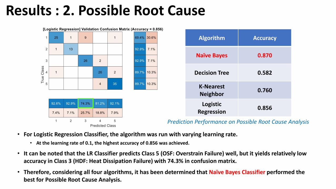
• For Logistic Regression Classifier, the algorithm was run with varying learning rate.

• At the learning rate of 0.1, the highest accuracy of 0.856 was achieved.

• It can be noted that the LR Classifier predicts Class 5 (OSF: Overstrain Failure) well, but it yields relatively low accuracy in Class 3 (HDF: Heat Dissipation Failure) with 74.3% in confusion matrix.

• Therefore, considering all four algorithms, it has been determined that Naïve Bayes Classifier performed the best for Possible Root Cause Analysis.

Results : 2. Possible Root Cause

• Thus, plotting all the possible root cause of the failure modes over the full dataset, as was expected in the beginning, the malfunctioning units reside in the “edges” of the accumulated regions (or in the “deviated regions”) as shown in the plots right.

• Interestingly, it was communicated that Class 2, 3, and 4 were hard to predict by the machine learning models. (having a relatively low accuracy.)

• The possible sources of error of why Class 2, 3, and 4 were hard to predict are as follows:

• For Class 3 and 4, as shown in Air Temperature and Process Temperature plots, it can be noted that Class 3 and 4 (Yellow and Purple) deeply reside in the accumulated regions (Class 1), making it harder for the models to distinguish the difference of Class 3 & 4 from Class 1.

• For Class 2, as shown in Air Temperature, Process Temperature, and Rotational Speed plots, it can be noted that Class 2 reside in the location that is too close to Class 1 and Class 5, making it harder for the models to distinguish the difference of Class 2 from Class 1 & 5.

ConclusionAlgorithm

Accuracy(Remaining Useful Life)

Accuracy(Possible Root Cause)

Naïve Bayes 0.994 0.870

Decision Tree 0.501 0.582

K-Nearest Neighbor 0.867 0.760

Logistic Regression 0.992 0.856

• Therefore, out of four algorithms to train the model for predicitve maintenance, it has been identified that Naive Bayes Classifier works the best for the current given dataset with an accuracy of 0.994 for Remaining Useful Life Analysis, and 0.870 for Possible Root Cause Analysis.

• The second algorithm that yields the best accuracy after Naive Bayes classifier is Logistic Regression Classifier – with proper time settings (learning rate), the performance of the LR could increase further.

• With the trained model on Reaming Useful Life Analysis, the equipment health can be monitored and determined to see if the maintenance should be performed or not.

• With the trained model on Possible Root Cause Analysis, when the failure occurs, this model will help the technicians on the site to choose the right set of maintenance actions to fix a failure.

Conclusion

𝑃 𝑦|𝑥 =𝑃 𝑦 𝑃 𝑥 𝑦

𝑃 𝑥≈𝑃 𝑦 ς𝑗=1

𝐷 𝑃 𝑥𝑗|𝑦

𝑃 𝑥

• I believe Naïve Bayes Classifier worked the best for the given dataset because of its unique assumption driven from “Bayes’ Theorem”.

• Looking at the distribution of the data as shown right and considering the nature of the data sources – a mechanical component, it can be clear that the features (Air Temp, Process Temp, etc.) in the given data are highly correlated to one another, making it harder for the models to distinguish the difference between the classes as we have talked about earlier in the slides.

• Thus, we need a classifier that trains the model without considering the correlation between the features in the data.

• Naïve Bayes Classifier exactly does this by using Bayes’ Theorem which assumes that the value of a particular feature is independent of the value of any other feature. (It is a strong (thus, naïve) independence assumption between the features.)

• And thus, when training the model with Naïve Bayes Classifier for this specific dataset, the performance of such model will generally be better than the other machine learning classifiers.

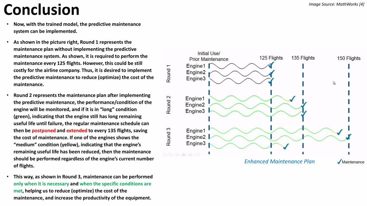
Conclusion• Now, with the trained model, the predictive maintenance

system can be implemented.

• As shown in the picture right, Round 1 represents the

maintenance plan without implementing the predictive

maintenance system. As shown, it is required to perform the

maintenance every 125 flights. However, this could be still

costly for the airline company. Thus, it is desired to implement

the predictive maintenance to reduce (optimize) the cost of the

maintenance.

• Round 2 represents the maintenance plan after implementing

the predictive maintenance, the performance/condition of the

engine will be monitored, and if it is in “long” condition

(green), indicating that the engine still has long remaining

useful life until failure, the regular maintenance schedule can

then be postponed and extended to every 135 flights, saving

the cost of maintenance. If one of the engines shows the

“medium” condition (yellow), indicating that the engine’s

remaining useful life has been reduced, then the maintenance

should be performed regardless of the engine’s current number

of flights.

• This way, as shown in Round 3, maintenance can be performed

only when it is necessary and when the specific conditions are

met, helping us to reduce (optimize) the cost of the

maintenance, and increase the productivity of the equipment.

Enhanced Maintenance Plan

Image Source: MathWorks [4]

• Like this, the benefits that predictive maintenance brings to the business are huge. It leads to…• Major Cost Savings (EX: Lower costs on maintenance

operations)

• Increased Availability of Systems

• Prolonged Equipment Life

• Reduced Downtime

• Increased Production Capacity

• Enhanced Safety

• Predicative Maintenance promises…[1]• 20 – 50% Reduction in time required to plan the maintenance.

• 10 – 20% Increase in equipment uptime and availability.

• 5 – 10% Reduction in overall maintenance cost.

ConclusionImage Source: Google

• It is highly recommended to explore the data refining technique. Most of time, the refinement of data increases the performance of any algorithm.

• For the given dataset, there was high imbalance in the distribution. Therefore, obtaining more data for other missing classes to balance the dataset would highly increase the model performance.

• Moreover, a self-tuning machine learning technique is also highly recommended to implement the model on the embedded system.

• Training & comparing with other various machine learning techniques would also widen the perspective and help the model selection.

• Lastly, for Remaining Useful Life Analysis, if the performance is low for the urgent classes, a cost matrix can be implemented to put more emphasis on the urgent class.

Future WorkImage Source: Google

Thank you

Citations / Resources• [1] Editor. “Predictive Maintenance: Employing IIoT and Machine Learning to Prevent Equipment

Failures.” AltexSoft, AltexSoft, www.altexsoft.com/blog/predictive-maintenance/.

• [2] Marktab. “Azure AI Guide for Predictive Maintenance Solutions - Team Data Science Process.” Team Data Science Process | Microsoft Docs, www.docs.microsoft.com/en-us/azure/machine-learning/team-data-science-process/predictive-maintenance-playbook/.

• [3] Gonfalonieri, Alexandre. “How to Implement Machine Learning For Predictive Maintenance.” Medium, Towards Data Science, www.towardsdatascience.com/how-to-implement-machine-learning-for-predictive-maintenance-4633cdbe4860/.

• [4] Filion Adam, “Predictive Maintenance: Unsupervised and Supervised Machine Learning.” MATLAB, Youtube, www.youtube.com/watch?v=AS0H43hMoWM

• [5] Daniele Apiletti, Claudia Barberis, Tania Cerquitelli, Alberto Macii, Enrico Macii, Massimo Poncino, and Francesco Ventura. “iSTEP, an integrated Self-Tuning Engine for Predictive maintenance in Industry 4.0” 2018 IEEE Computer Society, IEEE, 2018.