CS520: Stabiliy of constant coefficient problems (Ch. 4)
48
CS520: Stabiliy of constant coefficient problems (Ch. 4) Uri Ascher Department of Computer Science University of British Columbia [email protected] people.cs.ubc.ca/∼ascher/520.html Uri Ascher (UBC) CPSC 520: Difference methods (Ch. 4) Fall 2012 1 / 28
Transcript of CS520: Stabiliy of constant coefficient problems (Ch. 4)

CS520: Stabiliy of constant coefficientproblems (Ch. 4)
Uri Ascher
Department of Computer ScienceUniversity of British Columbia
people.cs.ubc.ca/∼ascher/520.html
Uri Ascher (UBC) CPSC 520: Difference methods (Ch. 4) Fall 2012 1 / 28
Constant coefficient PDE
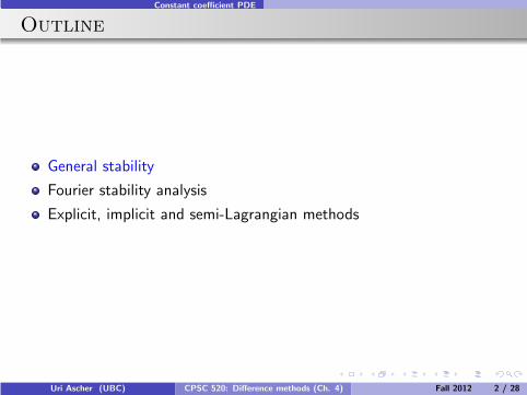
Outline
General stability
Fourier stability analysis
Explicit, implicit and semi-Lagrangian methods
Uri Ascher (UBC) CPSC 520: Difference methods (Ch. 4) Fall 2012 2 / 28
Constant coefficient PDE Recall
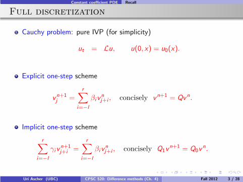
Full discretization
Cauchy problem: pure IVP (for simplicity)
ut = Lu, u(0, x) = u0(x).
Explicit one-step scheme
vn+1
j =r
∑
i=−l
βivnj+i , concisely vn+1 = Qvn.
Implicit one-step scheme
r∑
i=−l
γivn+1
j+i =r
∑
i=−l
βivnj+i , concisely Q1v
n+1 = Q0vn.
Uri Ascher (UBC) CPSC 520: Difference methods (Ch. 4) Fall 2012 3 / 28
Constant coefficient PDE Recall
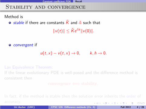
Stability and convergence
Method is
stable if there are constants K and α such that
‖v(t)‖ ≤ K eαt‖v(0)‖.
convergent if
u(t, x)− v(t, x) → 0, k , h → 0.
Lax Equivalence Theorem:If the linear evolutionary PDE is well-posed and the difference method isconsistent then
convergence ⇐⇒ stability.
In fact, if the method is stable then the solution error inherits the order ofaccuracy.
Uri Ascher (UBC) CPSC 520: Difference methods (Ch. 4) Fall 2012 4 / 28

Constant coefficient PDE Recall
Stability and convergence
Method is
stable if there are constants K and α such that
‖v(t)‖ ≤ K eαt‖v(0)‖.
convergent if
u(t, x)− v(t, x) → 0, k , h → 0.
Lax Equivalence Theorem:If the linear evolutionary PDE is well-posed and the difference method isconsistent then
convergence ⇐⇒ stability.
In fact, if the method is stable then the solution error inherits the order ofaccuracy.
Uri Ascher (UBC) CPSC 520: Difference methods (Ch. 4) Fall 2012 4 / 28

Constant coefficient PDE General stability
General linear stability
Generally, with Q = Q−1
1Q0, can write
vn+1 = Q(nk , h)vn = · · · = Πnl=0Q(lk , h)v0 = Sk,h(tn+1, 0)v
0.
The stability condition is
‖Πn−1
l=0Q(lk , h)‖ ≤ K eαnk ∀n, k , nk ≤ tf .
If Q does not depend on t
‖Q(h)n‖ ≤ K eαnk .
This is satisfied if for all k and h small enough,
‖Q‖ ≤ eαk = 1 + O(k).
Uri Ascher (UBC) CPSC 520: Difference methods (Ch. 4) Fall 2012 5 / 28
Constant coefficient PDE General stability
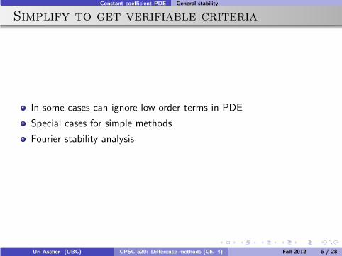
Simplify to get verifiable criteria
In some cases can ignore low order terms in PDE
Special cases for simple methods
Fourier stability analysis
Uri Ascher (UBC) CPSC 520: Difference methods (Ch. 4) Fall 2012 6 / 28
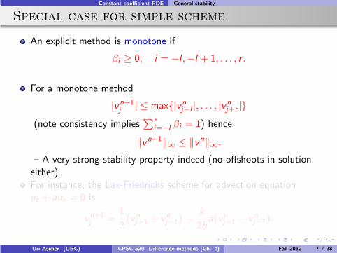
Constant coefficient PDE General stability
Special case for simple scheme
An explicit method is monotone if
βi ≥ 0, i = −l ,−l + 1, . . . , r .
For a monotone method
|vn+1
j | ≤ max{|vnj−l |, . . . , |vnj+r |}(note consistency implies
∑ri=−l βi = 1) hence
‖vn+1‖∞ ≤ ‖vn‖∞.
– A very strong stability property indeed (no offshoots in solutioneither).For instance, the Lax-Friedrichs scheme for advection equationut + aux = 0 is
vn+1
j =1
2
(
vnj+1 + vnj−1
)
− k
2ha(
vnj+1 − vnj−1
)
.
Uri Ascher (UBC) CPSC 520: Difference methods (Ch. 4) Fall 2012 7 / 28

Constant coefficient PDE General stability
Lax-Friedrichs scheme
The Lax-Friedrichs scheme for the advection equation ut + aux = 0 is
vn+1
j =1
2
(
vnj+1 + vnj−1
)
− k
2ha(
vnj+1 − vnj−1
)
.
It has accuracy order (1, 1), provided µ = k/h is fixed.
Assuming that the CFL condition holds, µ|a| ≤ 1, we have
β0 = 0, β±1 =1
2
(
1± µa)
≥ 0.
This is indeed a very stable scheme for hyperbolic PDEs
But it’s not very accurate. In fact, a monotone scheme is at mostfirst order accurate. Need a general-purpose recipe.
Uri Ascher (UBC) CPSC 520: Difference methods (Ch. 4) Fall 2012 8 / 28

Constant coefficient PDE
Outline
General stability
Fourier stability analysis
Explicit, implicit and semi-Lagrangian methods
Uri Ascher (UBC) CPSC 520: Difference methods (Ch. 4) Fall 2012 9 / 28
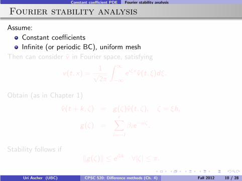
Constant coefficient PDE Fourier stability analysis
Fourier stability analysis
Assume:
Constant coefficients
Infinite (or periodic BC), uniform mesh
Then can consider v in Fourier space, satisfying
v(t, x) =1√2π
∫ ∞
−∞
eıξx v(t, ξ)dξ.
Obtain (as in Chapter 1)
v(t + k , ζ) = g(ζ)v(t, ζ), ζ = ξh,
g(ζ) =r
∑
i=−l
βie−ıiζ .
Stability follows if‖g(ζ)‖ ≤ eαk ∀|ζ| ≤ π.
Uri Ascher (UBC) CPSC 520: Difference methods (Ch. 4) Fall 2012 10 / 28
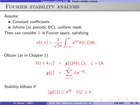
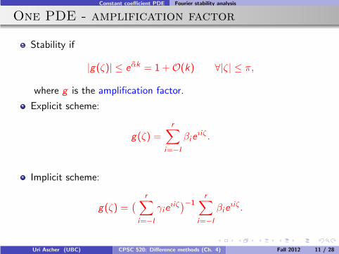
Constant coefficient PDE Fourier stability analysis
One PDE - amplification factor
Stability if
|g(ζ)| ≤ eαk = 1 +O(k) ∀|ζ| ≤ π,
where g is the amplification factor.
Explicit scheme:
g(ζ) =r
∑
i=−l
βieıiζ .
Implicit scheme:
g(ζ) =(
r∑
i=−l
γieıiζ)−1
r∑
i=−l
βieıiζ .
Uri Ascher (UBC) CPSC 520: Difference methods (Ch. 4) Fall 2012 11 / 28

Constant coefficient PDE Fourier stability analysis
Example: forward Euler for heat equation
For the simple heat equation
ut = uxx ,
apply centered 2nd order discretization in space:
dvj
dt=
1
h2D+D−vj .
Next discretize in time using forward Euler:
vn+1
j = vnj + µD+D−vnj ,
where µ = k/h2.
For the amplification factor, note
D+D−eıξx = (eıζ − 2 + e−ıζ)eıξx = 2(cos ζ − 1)eıξx
= −4 sin2(ζ/2)eıξx .
Uri Ascher (UBC) CPSC 520: Difference methods (Ch. 4) Fall 2012 12 / 28

Constant coefficient PDE Fourier stability analysis
Example: forward Euler for heat equation
Calculate amplification factor:
D+D−eıξx = (eıζ − 2 + e−ıζ)eıξx = 2(cos ζ − 1)eıξx
= −4 sin2(ζ/2)eıξx ,
sog(ζ) = 1− 4µ sin2(ζ/2).
To ensure stability require |g(ζ)| ≤ 1, so we must require
µ ≤ 1/2 i.e., k ≤ h2/2.
Note it is the high wave numbers ζ near ±π that cause problems firstif µ > 1/2. Also, although method order (1,2) is conducive to takingk ∼ h2, restricting µ ≤ .5 is for stability, not accuracy reasons.
Uri Ascher (UBC) CPSC 520: Difference methods (Ch. 4) Fall 2012 13 / 28
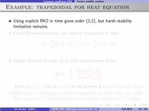
Constant coefficient PDE Fourier stability analysis
Example: trapezoidal for heat equation
Using explicit RK2 in time gives order (2,2), but harsh stabilitylimitation remains.
Crank-Nicolson method: use implicit trapezoidal in time.
(1− µ
2D+D−)v
n+1
j = (1 +µ
2D+D−)v
nj .
Obtain method of order (2,2) with amplification factor
g(ζ) =1− 2µ sin2(ζ/2)
1 + 2µ sin2(ζ/2).
Here |g(ζ)| ≤ 1 for all µ > 0, so the scheme is unconditionally stable.
Must solve a tridiagonal system of equations at each time step. Still,this requires O(J) flops whereas forward Euler requires O(J2) flops.
Uri Ascher (UBC) CPSC 520: Difference methods (Ch. 4) Fall 2012 14 / 28

Constant coefficient PDE Fourier stability analysis
Difference operator amplification
Fourier analysis of usual difference operators is standard (need not startfrom scratch each time):
Difference operator Contribution to g(ζ)
D+ eıζ − 1D− 1− e−ıζ
D0 2ı sin ζδ 2ı sin(ζ/2)
D+D− −4 sin2(ζ/2)
Uri Ascher (UBC) CPSC 520: Difference methods (Ch. 4) Fall 2012 15 / 28

Constant coefficient PDE Fourier stability analysis
Several PDEs - amplification matrix
Amplification factor becomes an s × s amplification matrix G (ζ)defined in the same way as g(ζ).
But checking ‖G (ζ)‖ for infintiely many ζ is still not very simple.
von Neumann condition: check the spectral radius
ρ(G (ζ)) ≤ eαk ∀|ζ| ≤ π.
This is necessary and alomst sufficient for stability.
Uri Ascher (UBC) CPSC 520: Difference methods (Ch. 4) Fall 2012 16 / 28
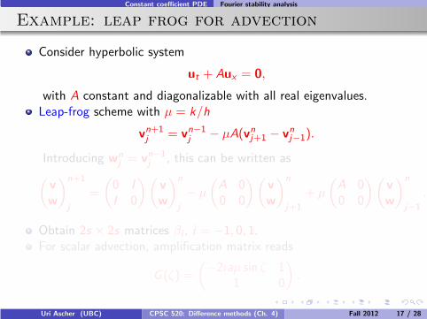
Constant coefficient PDE Fourier stability analysis
Example: leap frog for advection
Consider hyperbolic system
ut + Aux = 0,
with A constant and diagonalizable with all real eigenvalues.Leap-frog scheme with µ = k/h
vn+1
j = vn−1
j − µA(vnj+1 − vnj−1).
Introducing wnj = vn−1
j , this can be written as
(
vw
)n+1
j
=
(
0 I
I 0
)(
vw
)n
j
− µ
(
A 00 0
)(
vw
)n
j+1
+ µ
(
A 00 0
)(
vw
)n
j−1
.
Obtain 2s × 2s matrices βi , i = −1, 0, 1.For scalar advection, amplification matrix reads
G (ζ) =
(
−2ıaµ sin ζ 11 0
)
.
Uri Ascher (UBC) CPSC 520: Difference methods (Ch. 4) Fall 2012 17 / 28
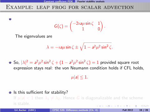
Constant coefficient PDE Fourier stability analysis
Example: leap frog for scalar advection
G (ζ) =
(
−2ıaµ sin ζ 11 0
)
.
The eigenvalues are
λ = −ıaµ sin ζ ±√
1− a2µ2 sin2 ζ.
So, |λ|2 = a2µ2 sin2 ζ + (1− a2µ2 sin2 ζ) = 1 provided square rootexpression stays real: the von Neumann condition holds if CFL holds,
µ|a| ≤ 1.
Is this sufficient for stability?If µ|a| < 1 then λ1 6= λ2. Hence G is diagonalizable and the schemeis stable.
Uri Ascher (UBC) CPSC 520: Difference methods (Ch. 4) Fall 2012 18 / 28
Constant coefficient PDE Fourier stability analysis
Example: leap frog for advection
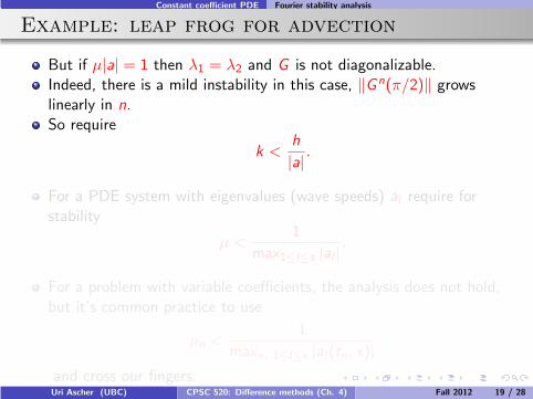
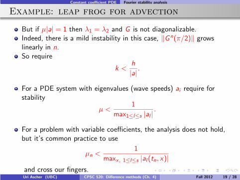
But if µ|a| = 1 then λ1 = λ2 and G is not diagonalizable.Indeed, there is a mild instability in this case, ‖Gn(π/2)‖ growslinearly in n.So require
k <h
|a| .
For a PDE system with eigenvalues (wave speeds) ai require forstability
µ <1
max1≤l≤s |al |.
For a problem with variable coefficients, the analysis does not hold,but it’s common practice to use
µn <1
maxx , 1≤l≤s |al(tn, x)|and cross our fingers.Uri Ascher (UBC) CPSC 520: Difference methods (Ch. 4) Fall 2012 19 / 28

Constant coefficient PDE Fourier stability analysis
Example: leap frog for advection
But if µ|a| = 1 then λ1 = λ2 and G is not diagonalizable.Indeed, there is a mild instability in this case, ‖Gn(π/2)‖ growslinearly in n.So require
k <h
|a| .
For a PDE system with eigenvalues (wave speeds) ai require forstability
µ <1
max1≤l≤s |al |.
For a problem with variable coefficients, the analysis does not hold,but it’s common practice to use
µn <1
maxx , 1≤l≤s |al(tn, x)|and cross our fingers.Uri Ascher (UBC) CPSC 520: Difference methods (Ch. 4) Fall 2012 19 / 28

Constant coefficient PDE Fourier stability analysis
Upwind scheme
For advection equation ut + aux = 0 recall one-sided scheme
vn+1
j = vnj − µa(
vnj+1 − vnj)
.
Fourier analysis gives amplification factor g(ζ) = 1− µa(
eıζ − 1)
,hence for stability, must require 0 ≤ µ(−a) ≤ 1.
What if a > 0? The forward difference in space gives anunconditionally unstable method, but backward difference in spacegives the scheme
vn+1
j = vnj − µa(
vnj − vnj−1
)
,
which for a > 0 is the mirror image of the forward scheme for a < 0.
So, more generally, use the upwind scheme
vn+1
j = vnj − µa
{
(
vnj+1− vnj
)
, a < 0(
vnj − vnj−1
)
, a > 0.
Uri Ascher (UBC) CPSC 520: Difference methods (Ch. 4) Fall 2012 20 / 28
Constant coefficient PDE Fourier stability analysis
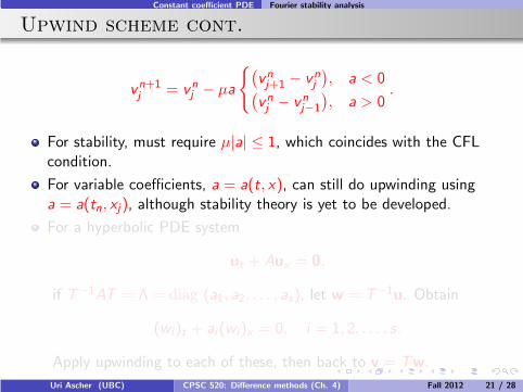
Upwind scheme cont.
vn+1
j = vnj − µa
{
(
vnj+1− vnj
)
, a < 0(
vnj − vnj−1
)
, a > 0.
For stability, must require µ|a| ≤ 1, which coincides with the CFLcondition.
For variable coefficients, a = a(t, x), can still do upwinding usinga = a(tn, xj), although stability theory is yet to be developed.
For a hyperbolic PDE system
ut + Aux = 0,
if T−1AT = Λ = diag (a1, a2, . . . , as), let w = T−1u. Obtain
(wi )t + ai (wi )x = 0, i = 1, 2, . . . , s.
Apply upwinding to each of these, then back to v = Tw.
Uri Ascher (UBC) CPSC 520: Difference methods (Ch. 4) Fall 2012 21 / 28

Constant coefficient PDE Fourier stability analysis
Upwind scheme cont.
vn+1
j = vnj − µa
{
(
vnj+1− vnj
)
, a < 0(
vnj − vnj−1
)
, a > 0.
For stability, must require µ|a| ≤ 1, which coincides with the CFLcondition.
For variable coefficients, a = a(t, x), can still do upwinding usinga = a(tn, xj), although stability theory is yet to be developed.
For a hyperbolic PDE system
ut + Aux = 0,
if T−1AT = Λ = diag (a1, a2, . . . , as), let w = T−1u. Obtain
(wi )t + ai (wi )x = 0, i = 1, 2, . . . , s.
Apply upwinding to each of these, then back to v = Tw.
Uri Ascher (UBC) CPSC 520: Difference methods (Ch. 4) Fall 2012 21 / 28
Constant coefficient PDE Fourier stability analysis
Outline
General stability
Fourier stability analysis
Explicit, implicit and semi-Lagrangian methods
Uri Ascher (UBC) CPSC 520: Difference methods (Ch. 4) Fall 2012 22 / 28
Constant coefficient PDE Semi-Lagrangian
Explicit vs implicit methods
The explicit methods we saw, both for ODEs and for PDEs, all havestability restrictions, limiting the time step k for a given spatial step h.
There are implicit methods (e.g., Crank-Nicolson) that areunconditionally stable, i.e., k not limited by stability considerations.However, for nonlinear problems in several space dimensions, solvingresulting algebraic problem can become expensive.
Recall the CFL condition: the domain of dependence of the PDEmust be contained in the domain of dependence of the differencescheme. This suggests (for hyperbolic PDEs) that all explicit schemeshave finite stability restrictions, whereas implicit schemes can beunconditionally stable.
Uri Ascher (UBC) CPSC 520: Difference methods (Ch. 4) Fall 2012 23 / 28

Constant coefficient PDE Semi-Lagrangian
Eulerian vs Lagrangian
Eulerian approach: stationary observer on a grid observing fluidflowing by.Pro: easiest to handle book-keeping, develop general methods, etc.Con: stability restriction on time step, occasionally excessive artificialdiffusion/viscosity.
Lagrangian approach: observer sits on a fluid particle flowing along acharacteristic curve.Pro: clean solutions, no stability restrictions, avoid certain boundarydifficulties.Con: may not have good solution everywhere, more difficultbook-keeping.
Semi-Lagrangian: attempt to combine the best of both worlds byfollowing characteristics backwards from a grid at the unknown timelevel.
Uri Ascher (UBC) CPSC 520: Difference methods (Ch. 4) Fall 2012 24 / 28

Constant coefficient PDE Semi-Lagrangian
Example: simplest advection
Recall: for ut + aux = 0, a < 0, have CFL compatibility if µ|a| ≤ 1.
0 x
t
.2 .4 .6 .8 1
.25
.5
.75
1
Uri Ascher (UBC) CPSC 520: Difference methods (Ch. 4) Fall 2012 25 / 28
Constant coefficient PDE Semi-Lagrangian
Recall one-sided scheme
For advection equation ut + aux = 0 consider one-sided scheme
vn+1
j = vnj − µa(
vnj+1 − vnj)
.
Fourier analysis gives amplification factor g(ζ) = 1− µa(
eıζ − 1)
.
For stability, require amplification factor to satisfy
|g(ζ)| ≤ 1, −π ≤ ζ ≤ π
hence must require 0 ≤ µ(−a) ≤ 1, i.e., that CFL hold.
Can interpret this method as semi-Lagrangian: trace characteristic at(tn+1, xj) to its foor at tn, which is at x∗ = (−a)µxj+1 + (1 + aµ)xj .Then interpolate linearly
vn∗ = (−a)µvnj+1 + (1 + aµ)vnj
and set vn+1
j = vn∗ .
Uri Ascher (UBC) CPSC 520: Difference methods (Ch. 4) Fall 2012 26 / 28

Constant coefficient PDE Semi-Lagrangian
Semi-Lagrangian method
Extend this interpretation of the one-sided scheme by tracing thecharacteristic curve further back!
Imagine the one-sided scheme on a coarse grid with widths k = lk
and h = lh for some l ≥ 1.
Next, instead of interpolating between xj and xj+1 = xj + h, find νsuch that xν ≤ x∗ ≤ xν + h and interpolate v nν and v nν+1 linearly for
v∗. Then set this value to be v n+1
j as before. The new time step istherefore l times larger, with the same spatial mesh as before.
Now, although we may still declare lk(−a) = k(−a) ≤ h = lh, this isno longer binding because can increase l arbitrarily for the (k , h)mesh.
In other words, for a fixed h can take k arbitrarily large withoutstability concerns in this way!
Uri Ascher (UBC) CPSC 520: Difference methods (Ch. 4) Fall 2012 27 / 28

Constant coefficient PDE Semi-Lagrangian
Semi-Lagrangian method cont.
Can obviously extend this method automatically to a of any sign(automatic upwinding).
The described method has similar accuracy characteristics as theupwind method (in particular it is 1st order accurate), but can requiremuch less work.
Technically, need l → ∞ for unlimited stability, so it’s not really anunconditionally stable explicit scheme, mathematically speaking.
The above assessment relies more heavily on the special form of theconstant-coefficient, scalar PDE.
Uri Ascher (UBC) CPSC 520: Difference methods (Ch. 4) Fall 2012 28 / 28