CS483-10 Elementary Graph Algorithms &...
40
CS483-10 Elementary Graph Algorithms & Transform-and-Conquer Instructor: Fei Li Room 443 ST II Office hours: Tue. & Thur. 1:30pm - 2:30pm or by appointments [email protected] with subject: CS483 http://www.cs.gmu.edu/∼ lifei/teaching/cs483_fall07/ Based on Introduction to the Design and Analysis of Algorithms by Anany Levitin, Jyh-Ming Lien’s notes, and Introduction to Algorithms by CLRS. CS483 Design and Analysis of Algorithms 1 Lecture 09, September 27, 2007
Transcript of CS483-10 Elementary Graph Algorithms &...
CS483-10 Elementary Graph Algorithms &
Transform-and-Conquer
Instructor: Fei Li
Room 443 ST II
Office hours: Tue. & Thur. 1:30pm - 2:30pm or by appointments
[email protected] with subject: CS483
http://www.cs.gmu.edu/∼ lifei/teaching/cs483_fall07/
Based on Introduction to the Design and Analysis of Algorithms by Anany Levitin, Jyh-Ming Lien’s
notes, and Introduction to Algorithms by CLRS.
CS483 Design and Analysis of Algorithms 1 Lecture 09, September 27, 2007
Outline
➣ Depth-first Search – cont
➣ Topological Sort
➣ Transform-and-Conquer – Gaussian Elimination
CS483 Design and Analysis of Algorithms 2 Lecture 09, September 27, 2007
CS483 Design and Analysis of Algorithms 3 Lecture 09, September 27, 2007
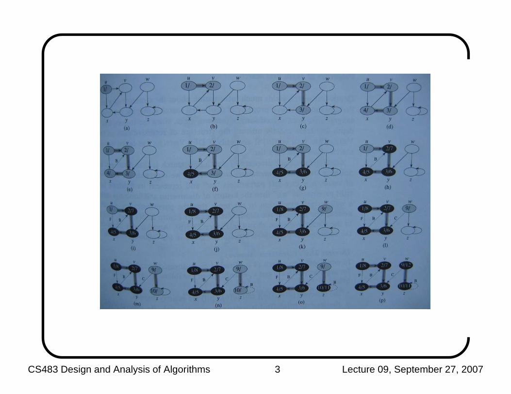
Depth-first Search (DFS)
➣ The correctness proof: Use an induction method
➣ The overall running time of DFS is O(|V |+ |E|).� The time initializing each vertex is O(|V |).� Each edge (u, v) ∈ E is examined twice, once exploring u and once
exploring v. Therefore takes O(|E|) time.
CS483 Design and Analysis of Algorithms 4 Lecture 09, September 27, 2007

Outline
➣ Depth-first Search – cont
➣ Topological Sort
➣ Transform-and-Conquer – Gaussian Elimination
CS483 Design and Analysis of Algorithms 5 Lecture 09, September 27, 2007
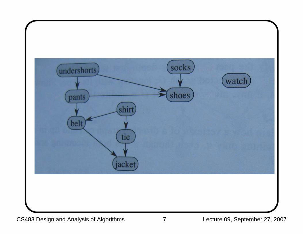
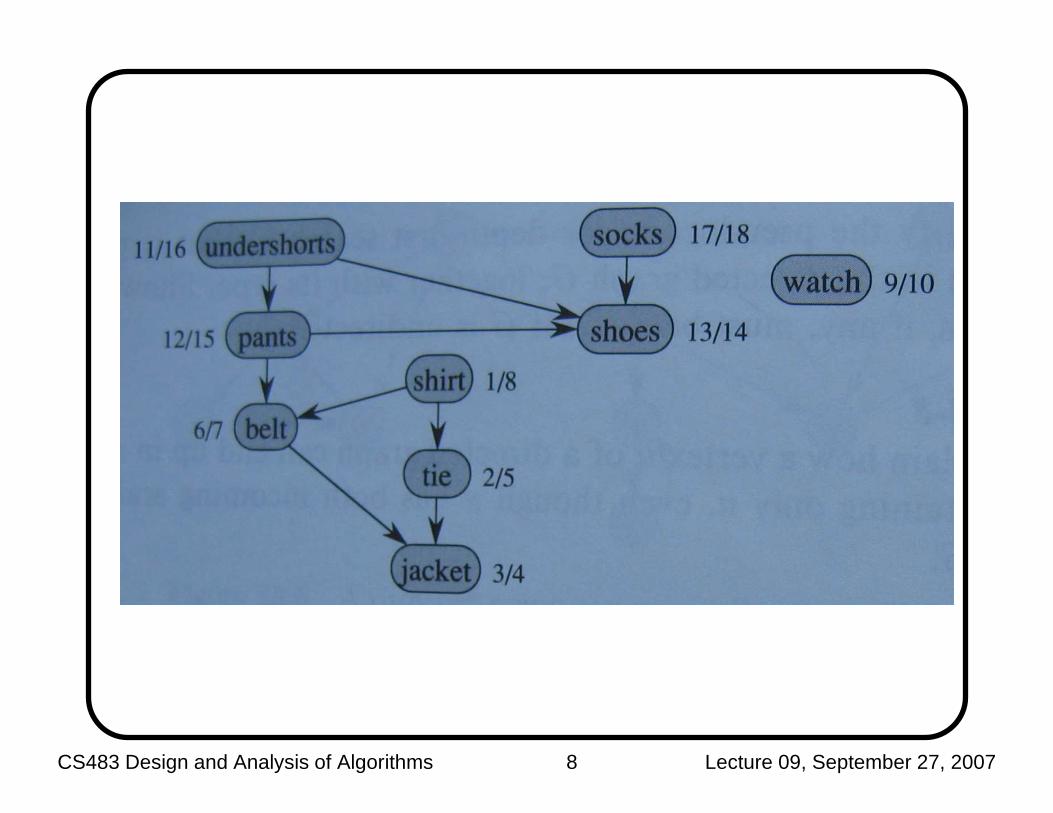
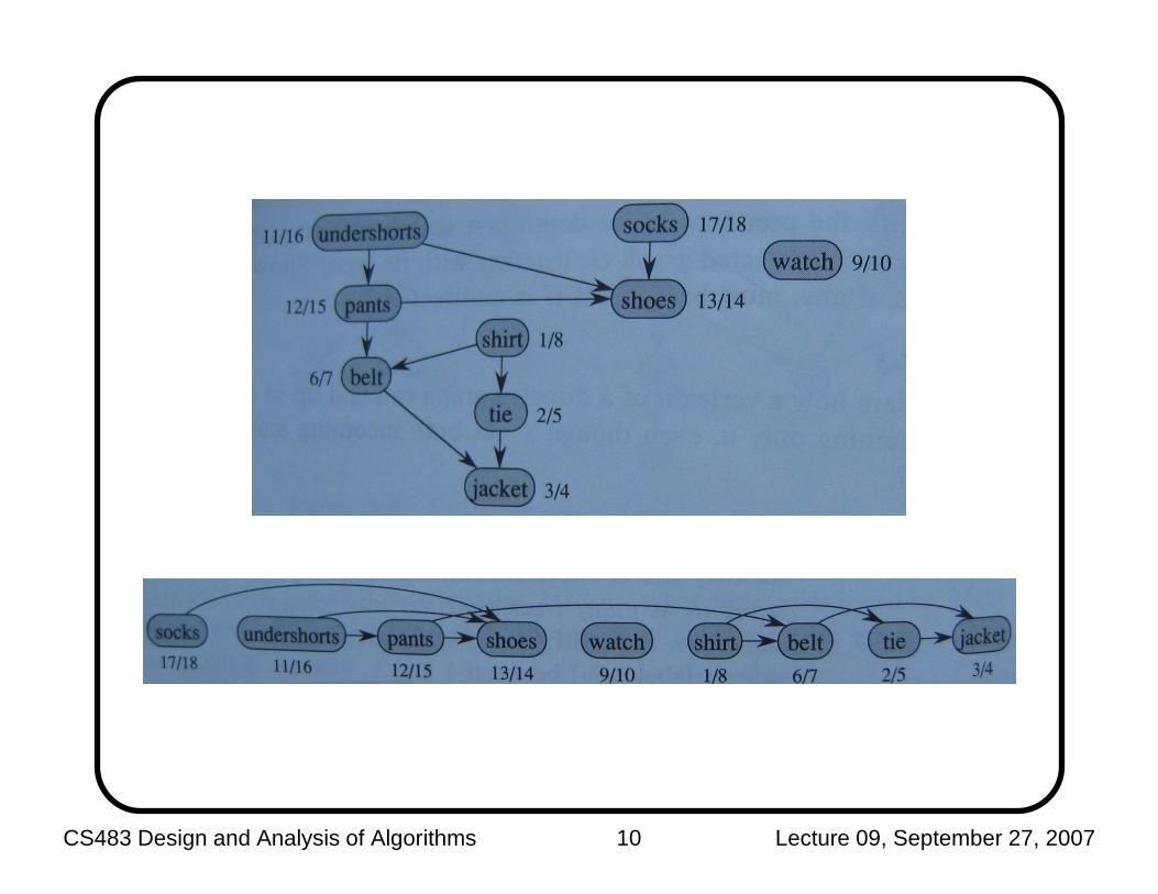
Topological Sort
➣ An application of DFS
➣ Input: a directed acyclic graph (DAG)
➣ Output: A linear ordering of all its vertices, such that if G contains an edge
(u, v), then, u appears before v in the ordering.
CS483 Design and Analysis of Algorithms 6 Lecture 09, September 27, 2007
CS483 Design and Analysis of Algorithms 7 Lecture 09, September 27, 2007
CS483 Design and Analysis of Algorithms 8 Lecture 09, September 27, 2007

Topological-Sort
Algorithm 0.1: TOPOLOGICAL-SORT(G(V, E))
Call DFS(G) to compute finishing times f [v] for each vertex v
As each vertex is finished, insert it onto the front of a linked list
return (the linked list of vertices)
CS483 Design and Analysis of Algorithms 9 Lecture 09, September 27, 2007
CS483 Design and Analysis of Algorithms 10 Lecture 09, September 27, 2007
Outline
➣ Depth-first Search – cont
➣ Topological Sort
➣ Transform-and-Conquer – Gaussian Elimination
CS483 Design and Analysis of Algorithms 11 Lecture 09, September 27, 2007
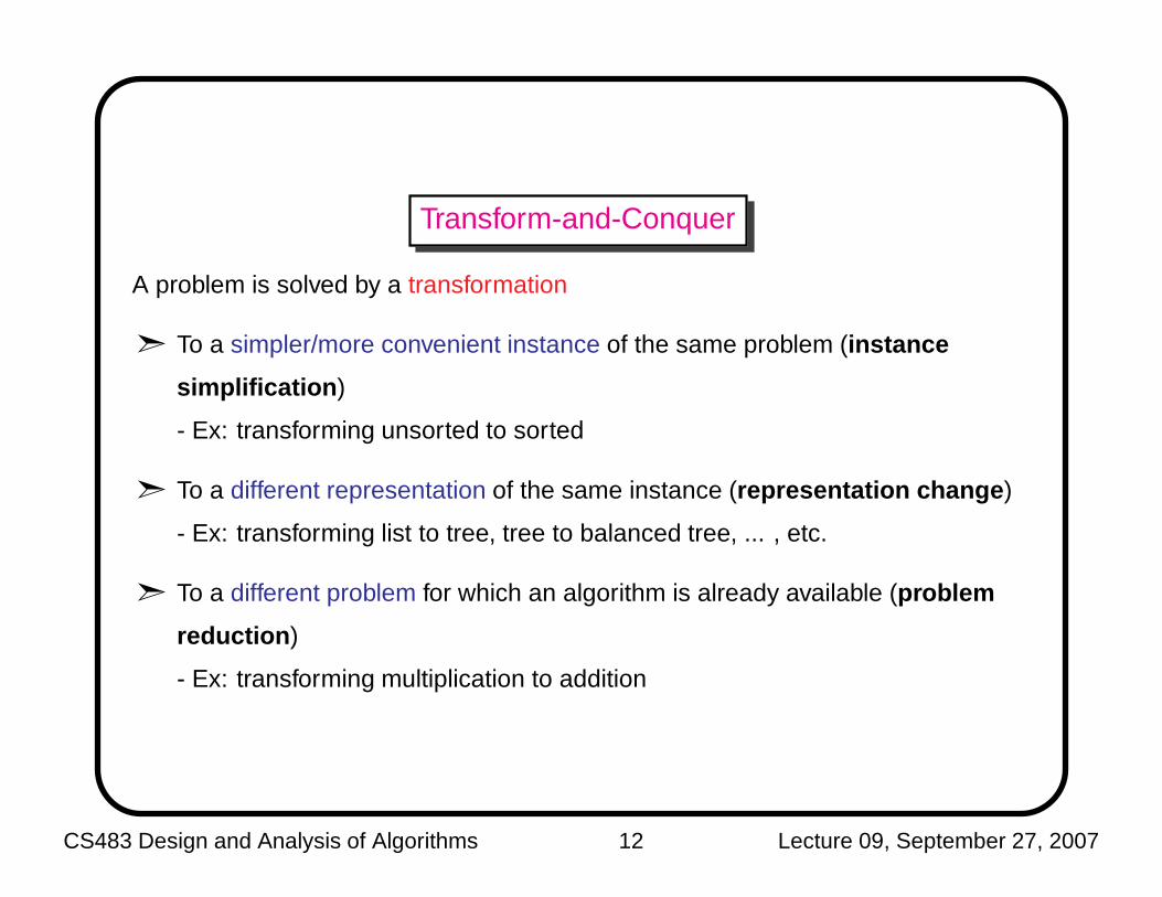
Transform-and-Conquer
A problem is solved by a transformation
➣ To a simpler/more convenient instance of the same problem (instance
simplification )
- Ex: transforming unsorted to sorted
➣ To a different representation of the same instance (representation change )
- Ex: transforming list to tree, tree to balanced tree, ... , etc.
➣ To a different problem for which an algorithm is already available (problem
reduction )
- Ex: transforming multiplication to addition
CS483 Design and Analysis of Algorithms 12 Lecture 09, September 27, 2007
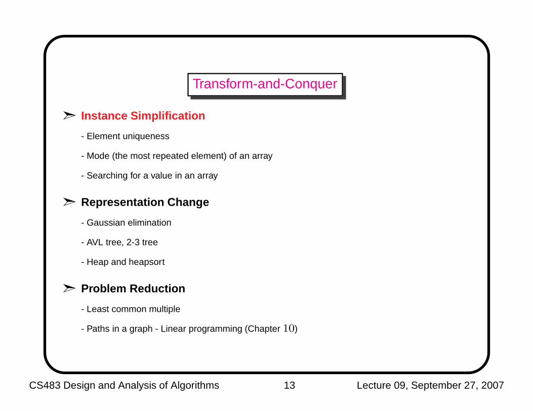
Transform-and-Conquer
➣ Instance Simplification
- Element uniqueness
- Mode (the most repeated element) of an array
- Searching for a value in an array
➣ Representation Change
- Gaussian elimination
- AVL tree, 2-3 tree
- Heap and heapsort
➣ Problem Reduction
- Least common multiple
- Paths in a graph - Linear programming (Chapter 10)
CS483 Design and Analysis of Algorithms 13 Lecture 09, September 27, 2007
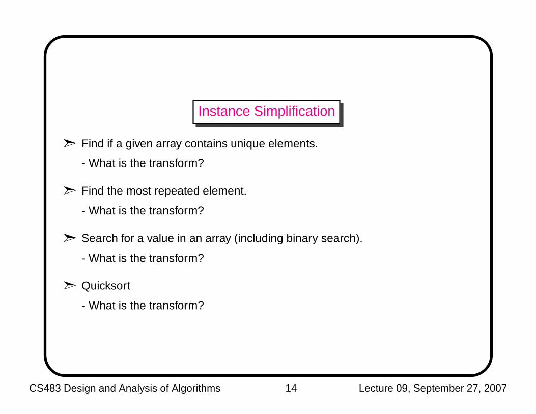
Instance Simplification
➣ Find if a given array contains unique elements.
- What is the transform?
➣ Find the most repeated element.
- What is the transform?
➣ Search for a value in an array (including binary search).
- What is the transform?
➣ Quicksort
- What is the transform?
CS483 Design and Analysis of Algorithms 14 Lecture 09, September 27, 2007
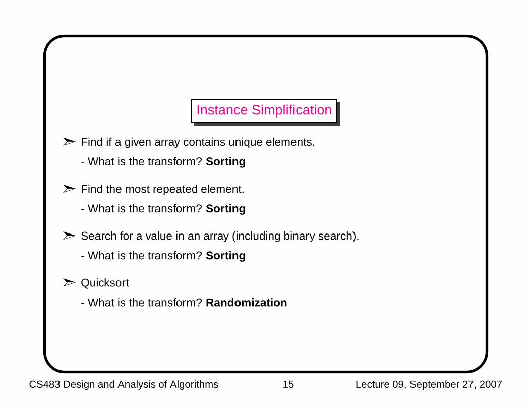
Instance Simplification
➣ Find if a given array contains unique elements.
- What is the transform? Sorting
➣ Find the most repeated element.
- What is the transform? Sorting
➣ Search for a value in an array (including binary search).
- What is the transform? Sorting
➣ Quicksort
- What is the transform? Randomization
CS483 Design and Analysis of Algorithms 15 Lecture 09, September 27, 2007

Instance Simplification - Presorting
Instance Simplification: Solve a problem’s instance by transforming it into another
simpler/easier instance of the same problem.
➣ Presorting
Many problems involving lists are easier when list is sorted.� Searching� Computing the median (selection problem)� Checking if all elements are distinct (element uniqueness)
Also:� Topological sorting helps solving some problems for directed Acyclic
graphs (DAGs).� Presorting is used in many geometric algorithms.
CS483 Design and Analysis of Algorithms 16 Lecture 09, September 27, 2007
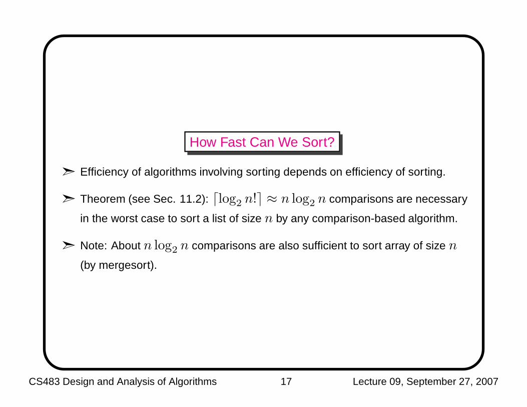
How Fast Can We Sort?
➣ Efficiency of algorithms involving sorting depends on efficiency of sorting.
➣ Theorem (see Sec. 11.2): ⌈log2 n!⌉ ≈ n log2 n comparisons are necessary
in the worst case to sort a list of size n by any comparison-based algorithm.
➣ Note: About n log2 n comparisons are also sufficient to sort array of size n
(by mergesort).
CS483 Design and Analysis of Algorithms 17 Lecture 09, September 27, 2007
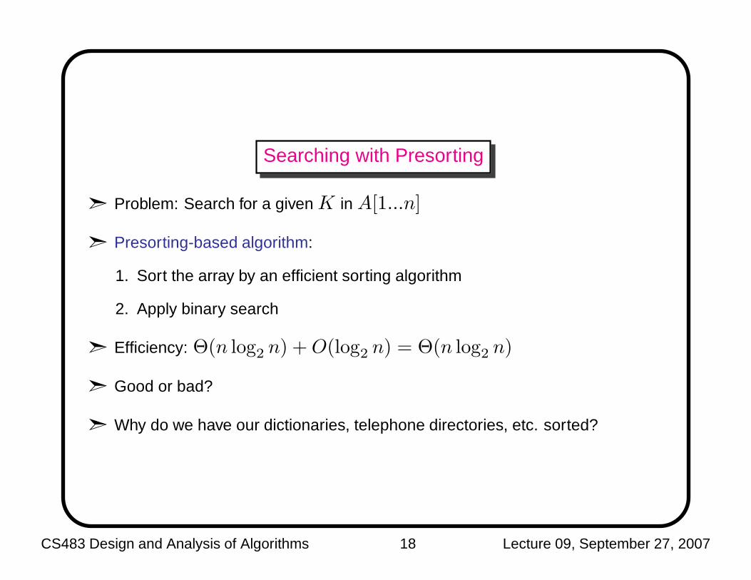
Searching with Presorting
➣ Problem: Search for a given K in A[1...n]
➣ Presorting-based algorithm:
1. Sort the array by an efficient sorting algorithm
2. Apply binary search
➣ Efficiency: Θ(n log2 n) + O(log2 n) = Θ(n log2 n)
➣ Good or bad?
➣ Why do we have our dictionaries, telephone directories, etc. sorted?
CS483 Design and Analysis of Algorithms 18 Lecture 09, September 27, 2007
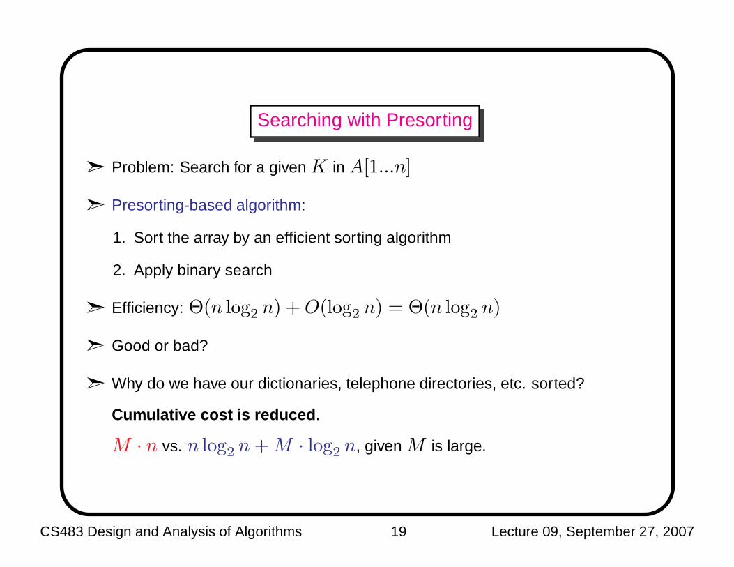
Searching with Presorting
➣ Problem: Search for a given K in A[1...n]
➣ Presorting-based algorithm:
1. Sort the array by an efficient sorting algorithm
2. Apply binary search
➣ Efficiency: Θ(n log2 n) + O(log2 n) = Θ(n log2 n)
➣ Good or bad?
➣ Why do we have our dictionaries, telephone directories, etc. sorted?
Cumulative cost is reduced .
M · n vs. n log2 n + M · log2 n, given M is large.
CS483 Design and Analysis of Algorithms 19 Lecture 09, September 27, 2007
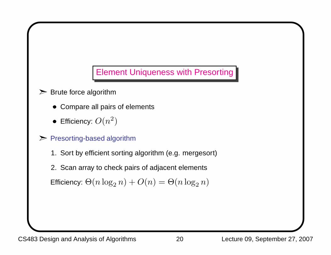
Element Uniqueness with Presorting
➣ Brute force algorithm� Compare all pairs of elements� Efficiency: O(n2)
➣ Presorting-based algorithm
1. Sort by efficient sorting algorithm (e.g. mergesort)
2. Scan array to check pairs of adjacent elements
Efficiency: Θ(n log2 n) + O(n) = Θ(n log2 n)
CS483 Design and Analysis of Algorithms 20 Lecture 09, September 27, 2007
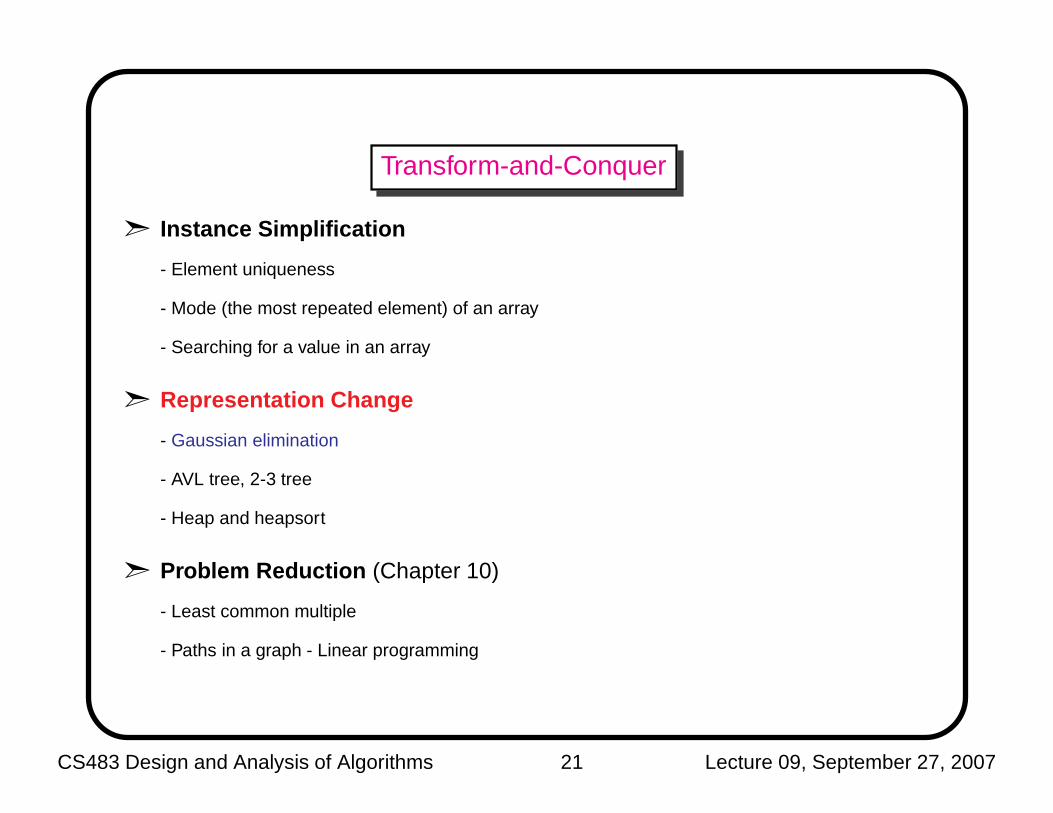
Transform-and-Conquer
➣ Instance Simplification
- Element uniqueness
- Mode (the most repeated element) of an array
- Searching for a value in an array
➣ Representation Change
- Gaussian elimination
- AVL tree, 2-3 tree
- Heap and heapsort
➣ Problem Reduction (Chapter 10)
- Least common multiple
- Paths in a graph - Linear programming
CS483 Design and Analysis of Algorithms 21 Lecture 09, September 27, 2007
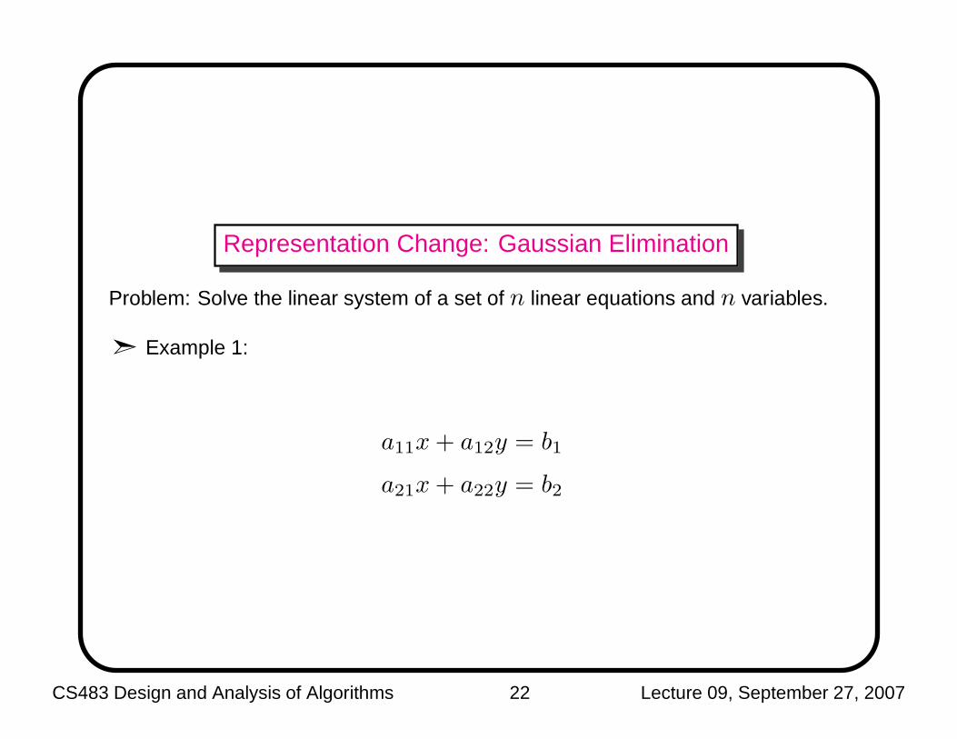
Representation Change: Gaussian Elimination
Problem: Solve the linear system of a set of n linear equations and n variables.
➣ Example 1:
a11x + a12y = b1
a21x + a22y = b2
CS483 Design and Analysis of Algorithms 22 Lecture 09, September 27, 2007
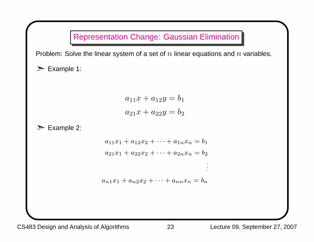
Representation Change: Gaussian Elimination
Problem: Solve the linear system of a set of n linear equations and n variables.
➣ Example 1:
a11x + a12y = b1
a21x + a22y = b2
➣ Example 2:
a11x1 + a12x2 + · · ·+ a1nxn = b1
a21x1 + a22x2 + · · ·+ a2nxn = b2
.
.
.
an1x1 + an2x2 + · · ·+ annxn = bn
CS483 Design and Analysis of Algorithms 23 Lecture 09, September 27, 2007

Representation Change: Gaussian Elimination
➣ Given: A system of n linear equations in n unknowns with an arbitrary
coefficient matrix.
➣ Transform to: An equivalent system of n linear equations in n unknowns with
an upper triangular coefficient matrix.
➣ Solve the latter by substitutions starting with the last equation and moving up
to the first one.
➣ Base: If we add a multiple of one equation to another, the overall system of
equations remains equivalent.
a11x1 + a12x2 + · · ·+ a1nxn = b1 a′
11x1 + a′
12x2 + · · ·+ a′
1nxn = b′1
a21x1 + a22x2 + · · ·+ a2nxn = b2 a′
22x2 + · · ·+ a′
2nxn = b′2...
.
.
.
an1x1 + an2x2 + · · ·+ annxn = bn a′
nnxn = b′n
CS483 Design and Analysis of Algorithms 24 Lecture 09, September 27, 2007
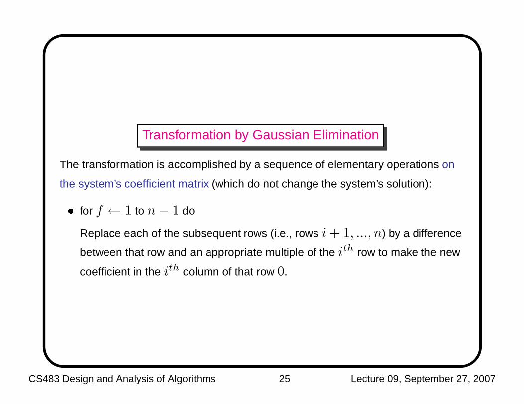
Transformation by Gaussian Elimination
The transformation is accomplished by a sequence of elementary operations on
the system’s coefficient matrix (which do not change the system’s solution):� for f ← 1 to n− 1 do
Replace each of the subsequent rows (i.e., rows i + 1, ..., n) by a difference
between that row and an appropriate multiple of the ith row to make the new
coefficient in the ith column of that row 0.
CS483 Design and Analysis of Algorithms 25 Lecture 09, September 27, 2007

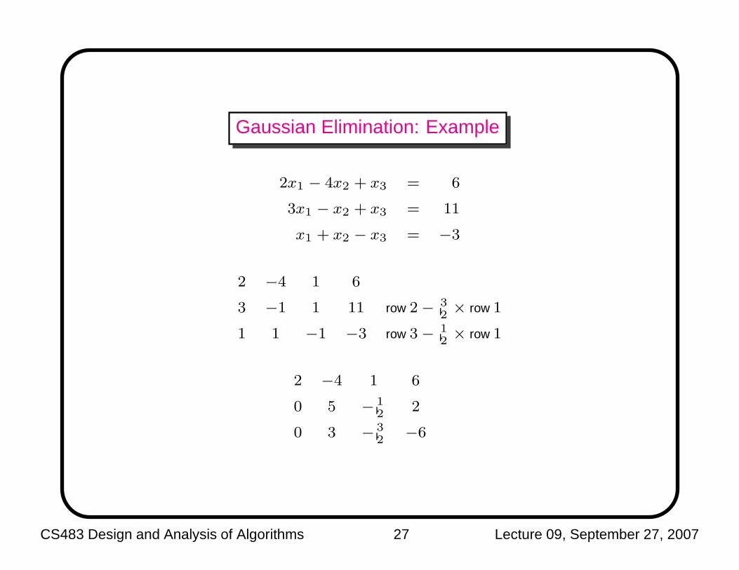
Gaussian Elimination: Example
2x1 − 4x2 + x3 = 6
3x1 − x2 + x3 = 11
x1 + x2 − x3 = −3
2 −4 1 6
3 −1 1 11
1 1 −1 −3
CS483 Design and Analysis of Algorithms 26 Lecture 09, September 27, 2007
Gaussian Elimination: Example
2x1 − 4x2 + x3 = 6
3x1 − x2 + x3 = 11
x1 + x2 − x3 = −3
2 −4 1 6
3 −1 1 11 row 2− 32× row 1
1 1 −1 −3 row 3− 12× row 1
2 −4 1 6
0 5 − 12
2
0 3 − 32−6
CS483 Design and Analysis of Algorithms 27 Lecture 09, September 27, 2007
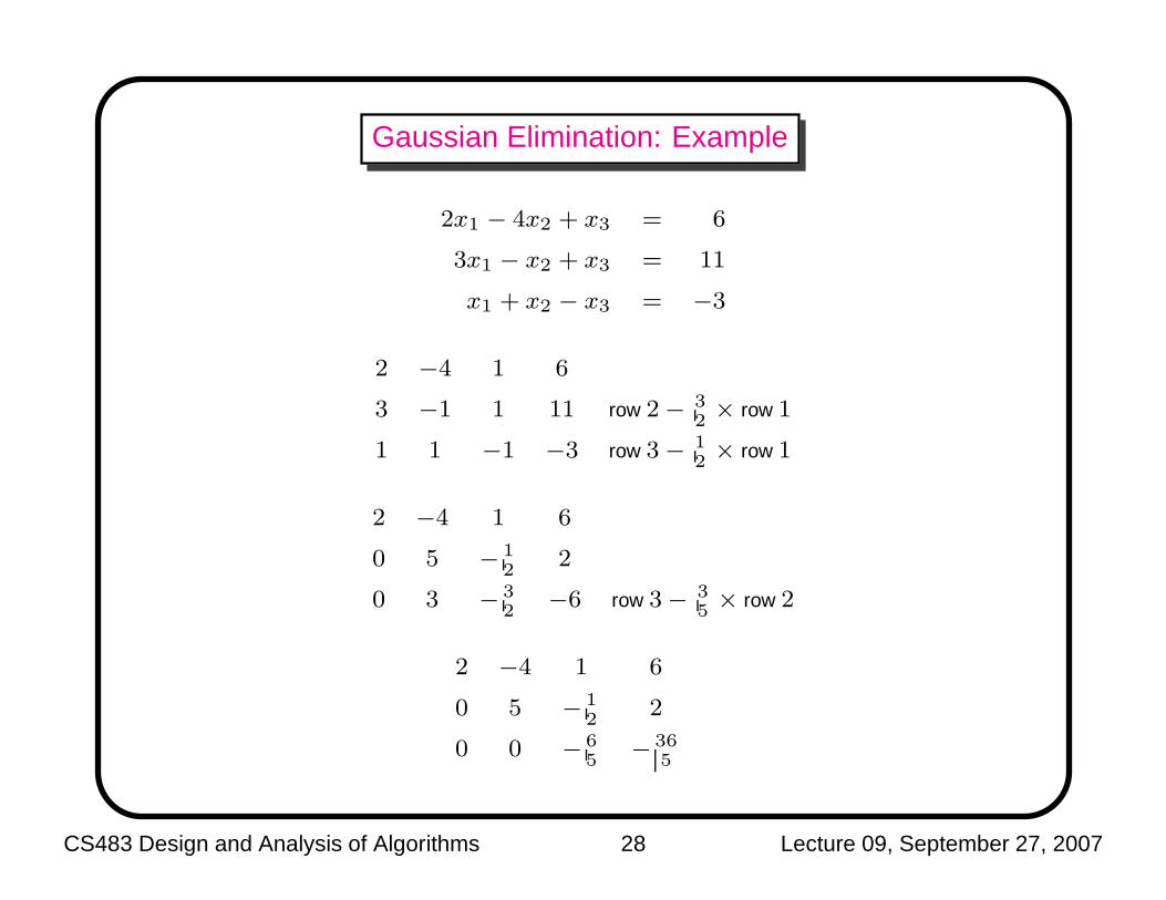
Gaussian Elimination: Example
2x1 − 4x2 + x3 = 6
3x1 − x2 + x3 = 11
x1 + x2 − x3 = −3
2 −4 1 6
3 −1 1 11 row 2− 32× row 1
1 1 −1 −3 row 3− 12× row 1
2 −4 1 6
0 5 − 12
2
0 3 − 32−6 row 3− 3
5× row 2
2 −4 1 6
0 5 − 12
2
0 0 − 65− 36
5
CS483 Design and Analysis of Algorithms 28 Lecture 09, September 27, 2007

Gaussian Elimination: Example
➣ We have:2x1 − 4x2 + x3 = 6
5x2 −12x3 = 2
− 65x3 = − 36
5
➣ Then we can solve x3, x2, x1 by backward substitution:
x3 = (− 365
)/(− 65) = 6
x2 = (2 + ( 12)× 6)/5 = 1
x1 = (66 + 4× 1)/2 = 2
CS483 Design and Analysis of Algorithms 29 Lecture 09, September 27, 2007

Gaussian Elimination Algorithm
Algorithm 0.2: GE(A[1 · · ·n, 1 · · ·n], b[1 · · ·n])
Append b to A as the last column
for i ∈ {1 · · ·n− 1}
do
for j ∈ {i + 1 · · ·n}
do
for k ∈ {j · · ·n}
do for A[j, k] = A[j, k]− A[i,k]A[j,i]A[i,i]
CS483 Design and Analysis of Algorithms 30 Lecture 09, September 27, 2007
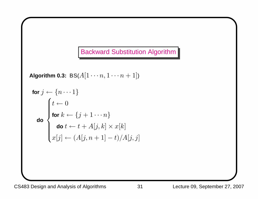
Backward Substitution Algorithm
Algorithm 0.3: BS(A[1 · · ·n, 1 · · ·n + 1])
for j ← {n · · · 1}
do
t← 0
for k ← {j + 1 · · ·n}
do t← t + A[j, k]× x[k]
x[j]← (A[j, n + 1]− t)/A[j, j]
CS483 Design and Analysis of Algorithms 31 Lecture 09, September 27, 2007
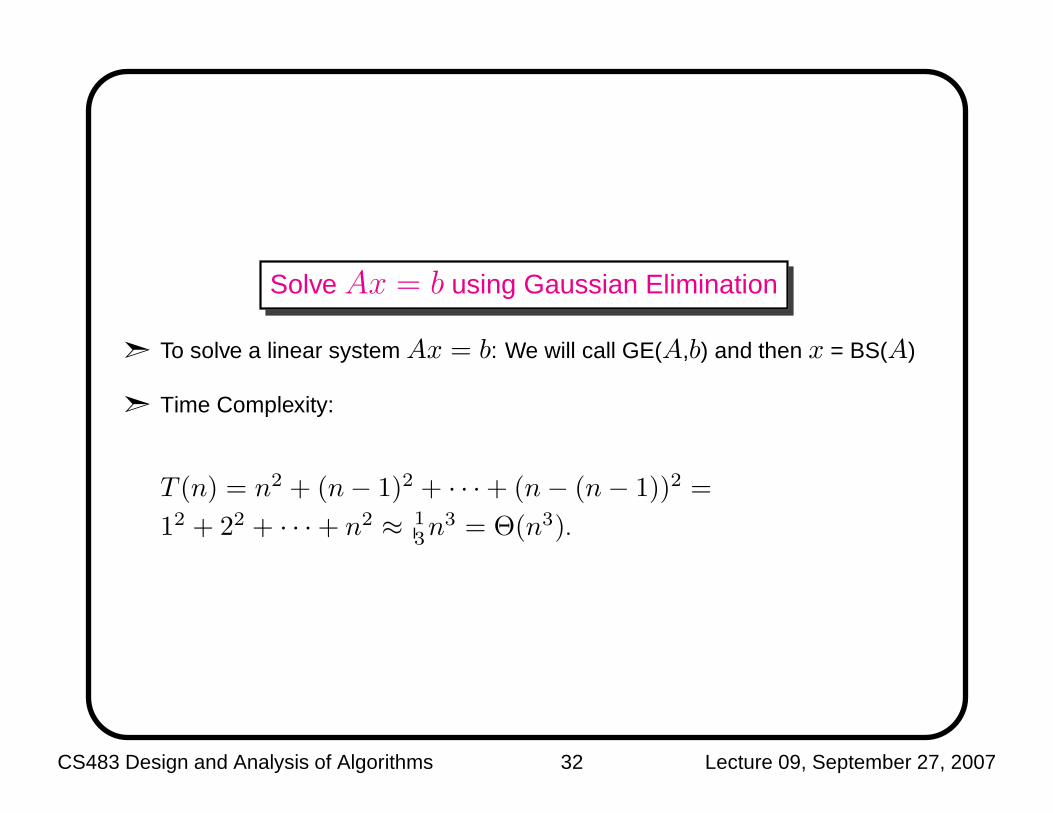
Solve Ax = b using Gaussian Elimination
➣ To solve a linear system Ax = b: We will call GE(A,b) and then x = BS(A)
➣ Time Complexity:
T (n) = n2 + (n− 1)2 + · · ·+ (n− (n− 1))2 =
12 + 22 + · · ·+ n2 ≈ 13n3 = Θ(n3).
CS483 Design and Analysis of Algorithms 32 Lecture 09, September 27, 2007
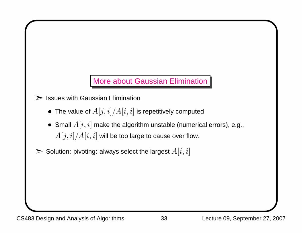
More about Gaussian Elimination
➣ Issues with Gaussian Elimination� The value of A[j, i]/A[i, i] is repetitively computed� Small A[i, i] make the algorithm unstable (numerical errors), e.g.,
A[j, i]/A[i, i] will be too large to cause over flow.
➣ Solution: pivoting: always select the largest A[i, i]
CS483 Design and Analysis of Algorithms 33 Lecture 09, September 27, 2007

Better Gaussian Elimination Algorithm
Algorithm 0.4: GE(A[1 · · ·n, 1 · · ·n], b[1 · · ·n])
Append b to A as the last column
for i ∈ {1 · · ·n− 1}
do
8
>
>
>
>
>
>
>
>
>
>
>
>
>
>
>
>
>
>
>
<
>
>
>
>
>
>
>
>
>
>
>
>
>
>
>
>
>
>
>
:
for j ∈ {i + 1 · · ·n}
do if |A[j, i]| > |A[pivot, i]|
then pivot← j
for j ∈ {i · · ·n + 1}
do swap(A[i, k], A[pivot, k])
for j ∈ {i + 1 · · ·n + 1}
do
8
>
>
<
>
>
:
temp←A[j,i]A[i,i]
for k ∈ {j · · ·n}
do for A[j, k] = A[j, k]−A[i, k]× temp
CS483 Design and Analysis of Algorithms 34 Lecture 09, September 27, 2007
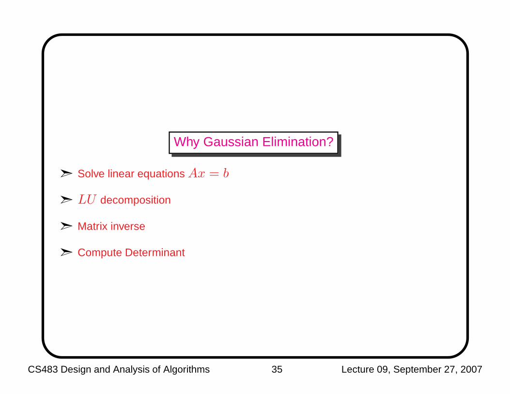
Why Gaussian Elimination?
➣ Solve linear equations Ax = b
➣ LU decomposition
➣ Matrix inverse
➣ Compute Determinant
CS483 Design and Analysis of Algorithms 35 Lecture 09, September 27, 2007
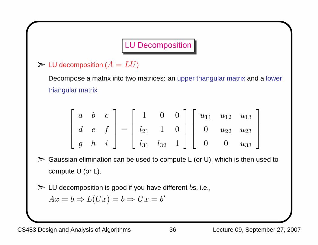
LU Decomposition
➣ LU decomposition (A = LU )
Decompose a matrix into two matrices: an upper triangular matrix and a lower
triangular matrix
a b c
d e f
g h i
=
1 0 0
l21 1 0
l31 l32 1
u11 u12 u13
0 u22 u23
0 0 u33
➣ Gaussian elimination can be used to compute L (or U), which is then used to
compute U (or L).
➣ LU decomposition is good if you have different bs, i.e.,
Ax = b⇒ L(Ux) = b⇒ Ux = b′
CS483 Design and Analysis of Algorithms 36 Lecture 09, September 27, 2007
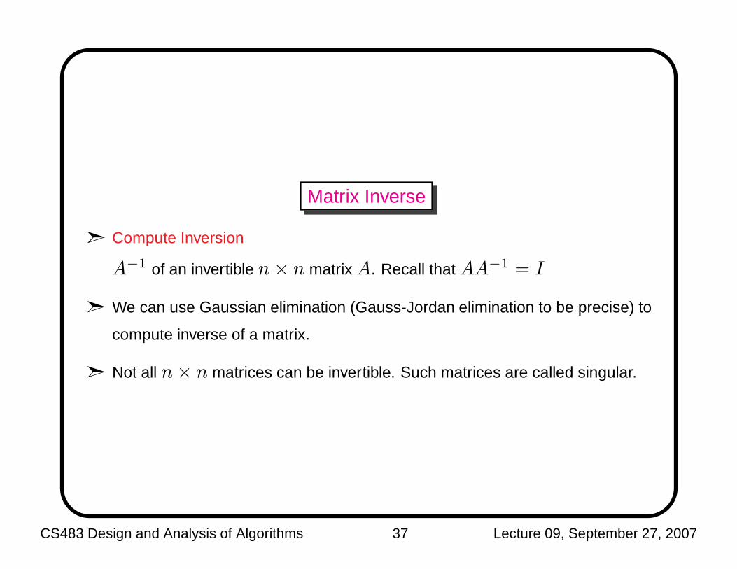
Matrix Inverse
➣ Compute Inversion
A−1 of an invertible n× n matrix A. Recall that AA−1 = I
➣ We can use Gaussian elimination (Gauss-Jordan elimination to be precise) to
compute inverse of a matrix.
➣ Not all n× n matrices can be invertible. Such matrices are called singular.
CS483 Design and Analysis of Algorithms 37 Lecture 09, September 27, 2007

Matrix Inverse
Example:
1 2
3 4
A−1 =
1 0
0 1
1 2
0 −2
A−1 =
1 0
−3 1
1 0
0 −2
A−1 =
−2 1
−3 1
1 0
0 1
A−1 =
−2 1
3/2 −1/2
CS483 Design and Analysis of Algorithms 38 Lecture 09, September 27, 2007
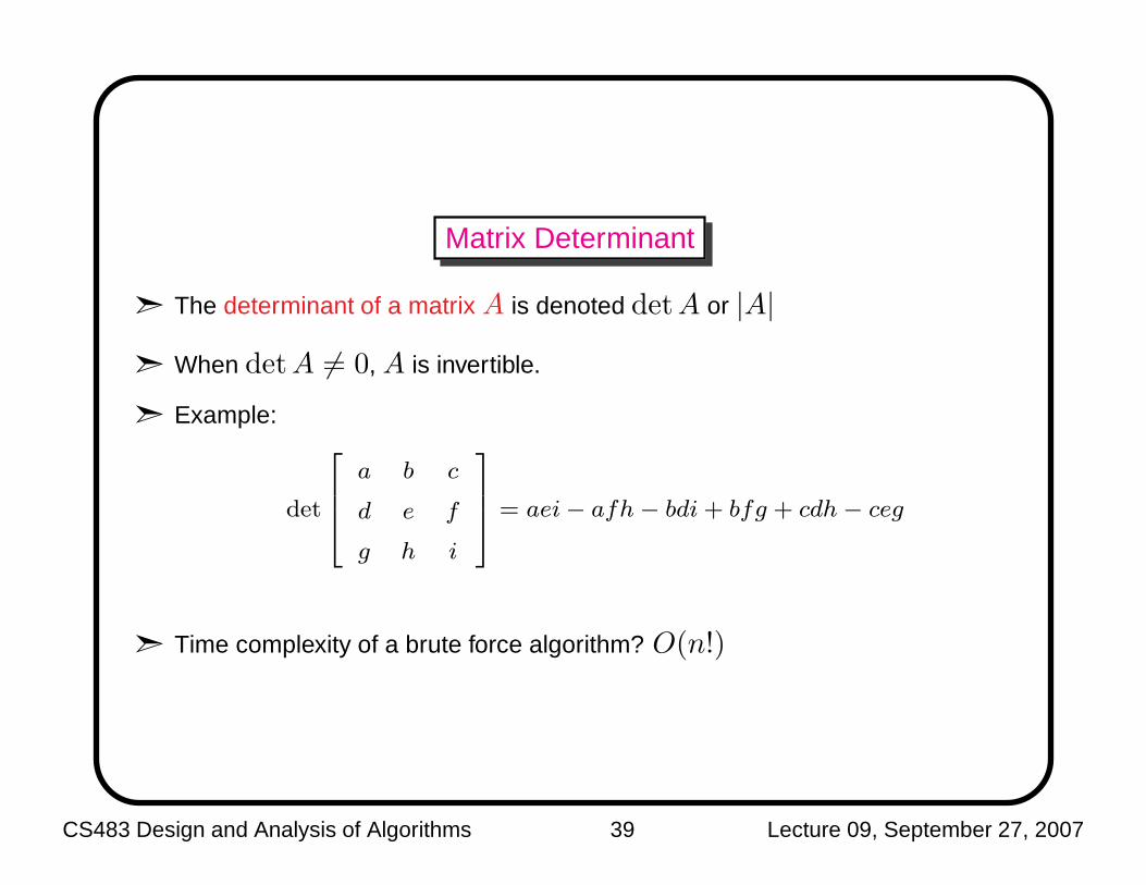
Matrix Determinant
➣ The determinant of a matrix A is denoted detA or |A|
➣ When detA 6= 0, A is invertible.
➣ Example:
det
2
6
6
4
a b c
d e f
g h i
3
7
7
5
= aei− afh− bdi + bfg + cdh− ceg
➣ Time complexity of a brute force algorithm? O(n!)
CS483 Design and Analysis of Algorithms 39 Lecture 09, September 27, 2007
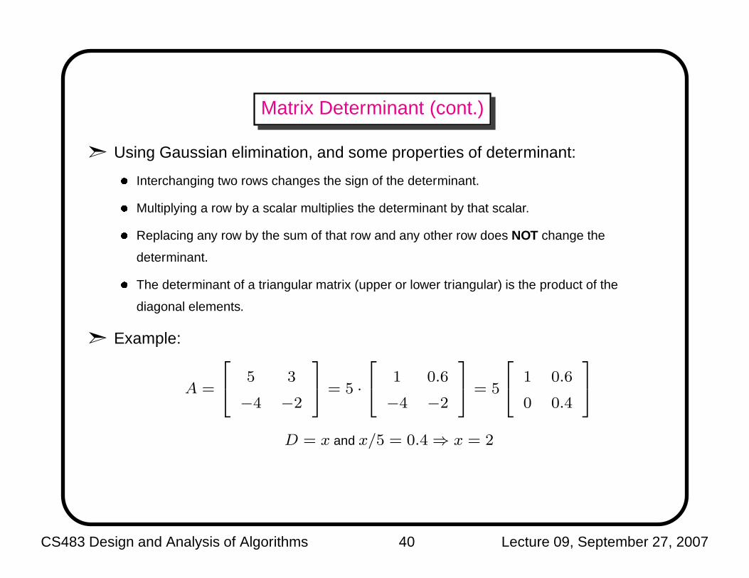
Matrix Determinant (cont.)
➣ Using Gaussian elimination, and some properties of determinant:� Interchanging two rows changes the sign of the determinant.� Multiplying a row by a scalar multiplies the determinant by that scalar.� Replacing any row by the sum of that row and any other row does NOT change the
determinant.� The determinant of a triangular matrix (upper or lower triangular) is the product of the
diagonal elements.
➣ Example:
A =
2
4
5 3
−4 −2
3
5 = 5 ·
2
4
1 0.6
−4 −2
3
5 = 5
2
4
1 0.6
0 0.4
3
5
D = x and x/5 = 0.4⇒ x = 2
CS483 Design and Analysis of Algorithms 40 Lecture 09, September 27, 2007