CS292F StatRL Lecture 5 RL Algorithms

Instructor: Yu-Xiang WangSpring 2021

UC Santa Barbara

1

Homeworks and Project

• Homework 0 “due” tonight• Sticking to the schedule is highly recommended

• You should start forming project team / ideas now• Did you check out the list of papers that I sent?

2

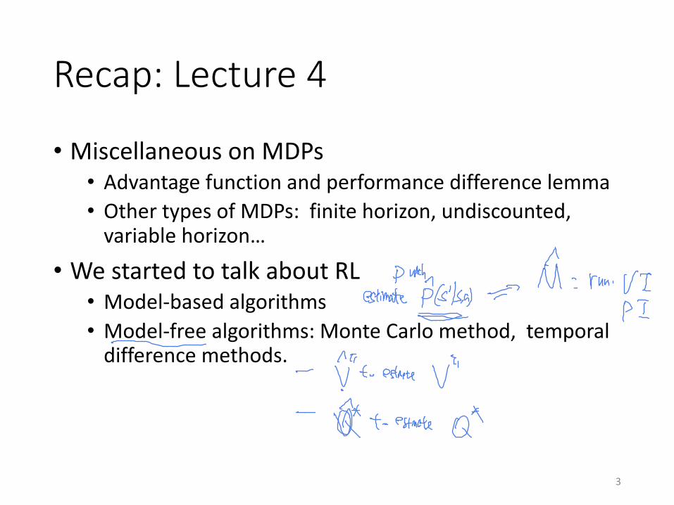
Recap: Lecture 4

• Miscellaneous on MDPs• Advantage function and performance difference lemma• Other types of MDPs: finite horizon, undiscounted,

variable horizon…

• We started to talk about RL• Model-based algorithms• Model-free algorithms: Monte Carlo method, temporal

difference methods.

3

Recap: MDP planning with access to generative models• Motivation:

1. Solving MDP faster / approximately with randomized algs that sample

2. Study sample complexity of RL with unknown transitions (without worrying about exploration)

• Algorithm of interest: Model-based plug-in estimator.• Sample all state-action pairs uniformly. Estimate the

transition kernel.• Do VI / PI on the approximate MDP.

4

Recap: “Monte Carlo” prediction / “Monte Carlo” control• Sutton and Barto notations / terminologies:• “Prediction” ó “Policy evaluation”• “Control” ó “Policy optimization”• Q and V are used to denotes estimates / while q, v

denotes the true value functions.• 0 based indexing: S0, A0, R1, S1, Asd, R2, …

• Idea: Roll out trajectories and average them.

5

Recap: Temporal Difference Learning

• Monte Carlo

• The idea of TD learning:

• TD-Policy evaluation

Issue: Gt can only be obtained after the entire episode!

We only need one step before we can plug-in and estimate the RHS!

Chapter 6

Temporal-Di↵erence Learning

If one had to identify one idea as central and novel to reinforcement learning, it would undoubtedly betemporal-di↵erence (TD) learning. TD learning is a combination of Monte Carlo ideas and dynamicprogramming (DP) ideas. Like Monte Carlo methods, TD methods can learn directly from raw expe-rience without a model of the environment’s dynamics. Like DP, TD methods update estimates basedin part on other learned estimates, without waiting for a final outcome (they bootstrap). The relation-ship between TD, DP, and Monte Carlo methods is a recurring theme in the theory of reinforcementlearning; this chapter is the beginning of our exploration of it. Before we are done, we will see thatthese ideas and methods blend into each other and can be combined in many ways. In particular, inChapter 7 we introduce n-step algorithms, which provide a bridge from TD to Monte Carlo methods,and in Chapter 12 we introduce the TD(�) algorithm, which seamlessly unifies them.

As usual, we start by focusing on the policy evaluation or prediction problem, the problem of esti-mating the value function v⇡ for a given policy ⇡. For the control problem (finding an optimal policy),DP, TD, and Monte Carlo methods all use some variation of generalized policy iteration (GPI). Thedi↵erences in the methods are primarily di↵erences in their approaches to the prediction problem.

6.1 TD Prediction

Both TD and Monte Carlo methods use experience to solve the prediction problem. Given someexperience following a policy ⇡, both methods update their estimate V of v⇡ for the nonterminal statesSt occurring in that experience. Roughly speaking, Monte Carlo methods wait until the return followingthe visit is known, then use that return as a target for V (St). A simple every-visit Monte Carlo methodsuitable for nonstationary environments is

V (St) V (St) + ↵hGt � V (St)

i, (6.1)

where Gt is the actual return following time t, and ↵ is a constant step-size parameter (c.f., Equation2.4). Let us call this method constant-↵ MC. Whereas Monte Carlo methods must wait until the endof the episode to determine the increment to V (St) (only then is Gt known), TD methods need to waitonly until the next time step. At time t + 1 they immediately form a target and make a useful updateusing the observed reward Rt+1 and the estimate V (St+1). The simplest TD method makes the update

V (St) V (St) + ↵hRt+1 + �V (St+1)� V (St)

i(6.2)

immediately on transition to St+1 and receiving Rt+1. In e↵ect, the target for the Monte Carlo updateis Gt, whereas the target for the TD update is Rt+1 + �V (St+1). This TD method is called TD(0), or

97

E⇡[Gt] = E⇡[Rt|St] + �V ⇡(St+1)<latexit sha1_base64="Btz+qqVUd+9ghQsBEaVf7eZr31s=">AAACNnicbVDLSsNAFJ34rPVVdelmsAhKoSQi6EYoiuhG8NUqNDFMptN26EwSZm6EEvNVbvwOd924UMStn+CkdqHWAwOHc+7lzjlBLLgG2x5YE5NT0zOzhbni/MLi0nJpZbWho0RRVqeRiNRtQDQTPGR14CDYbawYkYFgN0HvKPdv7pnSPAqvoR8zT5JOyNucEjCSXzpzJYFuEKTHmZ+6Mc+aJz54GB9gPOZc+vBwlbsV7HaIlAQ37obO1pWfQsXJtv1S2a7aQ+Bx4oxIGY1w7pee3VZEE8lCoIJo3XTsGLyUKOBUsKzoJprFhPZIhzUNDYlk2kuHsTO8aZQWbkfKvBDwUP25kRKpdV8GZjKPov96ufif10ygve+lPIwTYCH9PtROBIYI5x3iFleMgugbQqji5q+YdokiFEzTRVOC8zfyOGnsVB3DL3bLtcNRHQW0jjbQFnLQHqqhU3SO6oiiRzRAr+jNerJerHfr43t0whrtrKFfsD6/ABNcq3c=</latexit><latexit sha1_base64="Btz+qqVUd+9ghQsBEaVf7eZr31s=">AAACNnicbVDLSsNAFJ34rPVVdelmsAhKoSQi6EYoiuhG8NUqNDFMptN26EwSZm6EEvNVbvwOd924UMStn+CkdqHWAwOHc+7lzjlBLLgG2x5YE5NT0zOzhbni/MLi0nJpZbWho0RRVqeRiNRtQDQTPGR14CDYbawYkYFgN0HvKPdv7pnSPAqvoR8zT5JOyNucEjCSXzpzJYFuEKTHmZ+6Mc+aJz54GB9gPOZc+vBwlbsV7HaIlAQ37obO1pWfQsXJtv1S2a7aQ+Bx4oxIGY1w7pee3VZEE8lCoIJo3XTsGLyUKOBUsKzoJprFhPZIhzUNDYlk2kuHsTO8aZQWbkfKvBDwUP25kRKpdV8GZjKPov96ufif10ygve+lPIwTYCH9PtROBIYI5x3iFleMgugbQqji5q+YdokiFEzTRVOC8zfyOGnsVB3DL3bLtcNRHQW0jjbQFnLQHqqhU3SO6oiiRzRAr+jNerJerHfr43t0whrtrKFfsD6/ABNcq3c=</latexit><latexit sha1_base64="Btz+qqVUd+9ghQsBEaVf7eZr31s=">AAACNnicbVDLSsNAFJ34rPVVdelmsAhKoSQi6EYoiuhG8NUqNDFMptN26EwSZm6EEvNVbvwOd924UMStn+CkdqHWAwOHc+7lzjlBLLgG2x5YE5NT0zOzhbni/MLi0nJpZbWho0RRVqeRiNRtQDQTPGR14CDYbawYkYFgN0HvKPdv7pnSPAqvoR8zT5JOyNucEjCSXzpzJYFuEKTHmZ+6Mc+aJz54GB9gPOZc+vBwlbsV7HaIlAQ37obO1pWfQsXJtv1S2a7aQ+Bx4oxIGY1w7pee3VZEE8lCoIJo3XTsGLyUKOBUsKzoJprFhPZIhzUNDYlk2kuHsTO8aZQWbkfKvBDwUP25kRKpdV8GZjKPov96ufif10ygve+lPIwTYCH9PtROBIYI5x3iFleMgugbQqji5q+YdokiFEzTRVOC8zfyOGnsVB3DL3bLtcNRHQW0jjbQFnLQHqqhU3SO6oiiRzRAr+jNerJerHfr43t0whrtrKFfsD6/ABNcq3c=</latexit><latexit sha1_base64="Btz+qqVUd+9ghQsBEaVf7eZr31s=">AAACNnicbVDLSsNAFJ34rPVVdelmsAhKoSQi6EYoiuhG8NUqNDFMptN26EwSZm6EEvNVbvwOd924UMStn+CkdqHWAwOHc+7lzjlBLLgG2x5YE5NT0zOzhbni/MLi0nJpZbWho0RRVqeRiNRtQDQTPGR14CDYbawYkYFgN0HvKPdv7pnSPAqvoR8zT5JOyNucEjCSXzpzJYFuEKTHmZ+6Mc+aJz54GB9gPOZc+vBwlbsV7HaIlAQ37obO1pWfQsXJtv1S2a7aQ+Bx4oxIGY1w7pee3VZEE8lCoIJo3XTsGLyUKOBUsKzoJprFhPZIhzUNDYlk2kuHsTO8aZQWbkfKvBDwUP25kRKpdV8GZjKPov96ufif10ygve+lPIwTYCH9PtROBIYI5x3iFleMgugbQqji5q+YdokiFEzTRVOC8zfyOGnsVB3DL3bLtcNRHQW0jjbQFnLQHqqhU3SO6oiiRzRAr+jNerJerHfr43t0whrtrKFfsD6/ABNcq3c=</latexit>

Chapter 6

Temporal-Di↵erence Learning

If one had to identify one idea as central and novel to reinforcement learning, it would undoubtedly betemporal-di↵erence (TD) learning. TD learning is a combination of Monte Carlo ideas and dynamicprogramming (DP) ideas. Like Monte Carlo methods, TD methods can learn directly from raw expe-rience without a model of the environment’s dynamics. Like DP, TD methods update estimates basedin part on other learned estimates, without waiting for a final outcome (they bootstrap). The relation-ship between TD, DP, and Monte Carlo methods is a recurring theme in the theory of reinforcementlearning; this chapter is the beginning of our exploration of it. Before we are done, we will see thatthese ideas and methods blend into each other and can be combined in many ways. In particular, inChapter 7 we introduce n-step algorithms, which provide a bridge from TD to Monte Carlo methods,and in Chapter 12 we introduce the TD(�) algorithm, which seamlessly unifies them.

As usual, we start by focusing on the policy evaluation or prediction problem, the problem of esti-mating the value function v⇡ for a given policy ⇡. For the control problem (finding an optimal policy),DP, TD, and Monte Carlo methods all use some variation of generalized policy iteration (GPI). Thedi↵erences in the methods are primarily di↵erences in their approaches to the prediction problem.

6.1 TD Prediction

Both TD and Monte Carlo methods use experience to solve the prediction problem. Given someexperience following a policy ⇡, both methods update their estimate V of v⇡ for the nonterminal statesSt occurring in that experience. Roughly speaking, Monte Carlo methods wait until the return followingthe visit is known, then use that return as a target for V (St). A simple every-visit Monte Carlo methodsuitable for nonstationary environments is

V (St) V (St) + ↵hGt � V (St)

i, (6.1)

where Gt is the actual return following time t, and ↵ is a constant step-size parameter (c.f., Equation2.4). Let us call this method constant-↵ MC. Whereas Monte Carlo methods must wait until the endof the episode to determine the increment to V (St) (only then is Gt known), TD methods need to waitonly until the next time step. At time t + 1 they immediately form a target and make a useful updateusing the observed reward Rt+1 and the estimate V (St+1). The simplest TD method makes the update

V (St) V (St) + ↵hRt+1 + �V (St+1)� V (St)

i(6.2)

immediately on transition to St+1 and receiving Rt+1. In e↵ect, the target for the Monte Carlo updateis Gt, whereas the target for the TD update is Rt+1 + �V (St+1). This TD method is called TD(0), or

97

Bootstrapping!

6

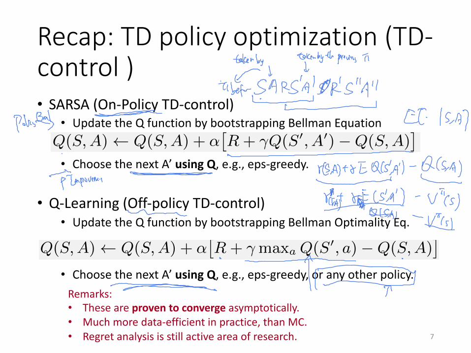
Recap: TD policy optimization (TD-control )• SARSA (On-Policy TD-control)

• Update the Q function by bootstrapping Bellman Equation

• Choose the next A’ using Q, e.g., eps-greedy.

• Q-Learning (Off-policy TD-control)• Update the Q function by bootstrapping Bellman Optimality Eq.

• Choose the next A’ using Q, e.g., eps-greedy, or any other policy.

7

106 CHAPTER 6. TEMPORAL-DIFFERENCE LEARNING

Exercise 6.8 Show that an action-value version of (6.6) holds for the action-value form of the TDerror �t = Rt+1 + �Q(St+1, At+1 � Q(St, At), again assuming that the values don’t change from step tostep. ⇤

It is straightforward to design an on-policy control algorithm based on the Sarsa prediction method.As in all on-policy methods, we continually estimate q⇡ for the behavior policy ⇡, and at the same timechange ⇡ toward greediness with respect to q⇡. The general form of the Sarsa control algorithm is givenin the box below.

Sarsa (on-policy TD control) for estimating Q ⇡ q⇤

Initialize Q(s, a), for all s 2 S, a 2 A(s), arbitrarily, and Q(terminal-state, ·) = 0Repeat (for each episode):

Initialize S

Choose A from S using policy derived from Q (e.g., ✏-greedy)Repeat (for each step of episode):

Take action A, observe R, S0

Choose A0 from S

0 using policy derived from Q (e.g., ✏-greedy)Q(S, A) Q(S, A) + ↵

⇥R + �Q(S0

, A0)�Q(S, A)

⇤

S S0; A A

0;until S is terminal

The convergence properties of the Sarsa algorithm depend on the nature of the policy’s dependenceon Q. For example, one could use "-greedy or "-soft policies. Sarsa converges with probability 1 to anoptimal policy and action-value function as long as all state–action pairs are visited an infinite numberof times and the policy converges in the limit to the greedy policy (which can be arranged, for example,with "-greedy policies by setting " = 1/t).

Example 6.5: Windy Gridworld Shown inset in Figure 6.3 is a standard gridworld, with start andgoal states, but with one di↵erence: there is a crosswind upward through the middle of the grid. Theactions are the standard four—up, down, right, and left—but in the middle region the resultantnext states are shifted upward by a “wind,” the strength of which varies from column to column. Thestrength of the wind is given below each column, in number of cells shifted upward. For example, ifyou are one cell to the right of the goal, then the action left takes you to the cell just above the goal.Let us treat this as an undiscounted episodic task, with constant rewards of �1 until the goal state isreached.

0 1000 2000 3000 4000 5000 6000 7000 8000

0

50

100

150

170

Episodes

Time steps

S G

0 0 0 01 1 1 12 2

Actions

Figure 6.3: Results of Sarsa applied to a gridworld (shown inset) in which movement is altered by a location-dependent, upward “wind.” A trajectory under the optimal policy is also shown.

6.5. Q-LEARNING: OFF-POLICY TD CONTROL 107

The graph in Figure 6.3 shows the results of applying "-greedy Sarsa to this task, with " = 0.1,↵ = 0.5, and the initial values Q(s, a) = 0 for all s, a. The increasing slope of the graph showsthat the goal is reached more and more quickly over time. By 8000 time steps, the greedy policywas long since optimal (a trajectory from it is shown inset); continued "-greedy exploration kept theaverage episode length at about 17 steps, two more than the minimum of 15. Note that Monte Carlomethods cannot easily be used on this task because termination is not guaranteed for all policies.If a policy was ever found that caused the agent to stay in the same state, then the next episodewould never end. Step-by-step learning methods such as Sarsa do not have this problem becausethey quickly learn during the episode that such policies are poor, and switch to something else.

Exercise 6.9: Windy Gridworld with King’s Moves Re-solve the windy gridworld task assuming eightpossible actions, including the diagonal moves, rather than the usual four. How much better can you dowith the extra actions? Can you do even better by including a ninth action that causes no movementat all other than that caused by the wind? ⇤Exercise 6.10: Stochastic Wind Re-solve the windy gridworld task with King’s moves, assumingthat the e↵ect of the wind, if there is any, is stochastic, sometimes varying by 1 from the mean valuesgiven for each column. That is, a third of the time you move exactly according to these values, as inthe previous exercise, but also a third of the time you move one cell above that, and another third ofthe time you move one cell below that. For example, if you are one cell to the right of the goal andyou move left, then one-third of the time you move one cell above the goal, one-third of the time youmove two cells above the goal, and one-third of the time you move to the goal. ⇤

6.5 Q-learning: O↵-policy TD Control

One of the early breakthroughs in reinforcement learning was the development of an o↵-policy TDcontrol algorithm known as Q-learning (Watkins, 1989), defined by

Q(St, At) Q(St, At) + ↵hRt+1 + � max

a

Q(St+1, a)�Q(St, At)i. (6.8)

In this case, the learned action-value function, Q, directly approximates q⇤, the optimal action-valuefunction, independent of the policy being followed. This dramatically simplifies the analysis of thealgorithm and enabled early convergence proofs. The policy still has an e↵ect in that it determineswhich state–action pairs are visited and updated. However, all that is required for correct convergenceis that all pairs continue to be updated. As we observed in Chapter 5, this is a minimal requirementin the sense that any method guaranteed to find optimal behavior in the general case must require it.Under this assumption and a variant of the usual stochastic approximation conditions on the sequenceof step-size parameters, Q has been shown to converge with probability 1 to q⇤.

Q-learning (o↵-policy TD control) for estimating ⇡ ⇡ ⇡⇤

Initialize Q(s, a), for all s 2 S, a 2 A(s), arbitrarily, and Q(terminal-state, ·) = 0Repeat (for each episode):

Initialize S

Repeat (for each step of episode):Choose A from S using policy derived from Q (e.g., ✏-greedy)Take action A, observe R, S

0

Q(S, A) Q(S, A) + ↵⇥R + � maxa Q(S0

, a)�Q(S, A)⇤

S S0

until S is terminalRemarks:• These are proven to converge asymptotically.• Much more data-efficient in practice, than MC.• Regret analysis is still active area of research.

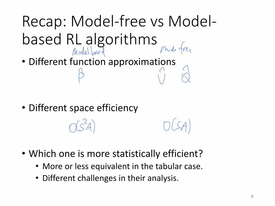
Recap: Model-free vs Model-based RL algorithms• Different function approximations

• Different space efficiency

• Which one is more statistically efficient?• More or less equivalent in the tabular case.• Different challenges in their analysis.

8

This lecture

• Variants / improvements of Sarsa and Q-learning

• TD-learning with function approximation

• Policy gradient methods

9

Expected SARSA

10

Expected SARSA

11

6.6. EXPECTED SARSA 109

Q-learning Expected Sarsa

Figure 6.5: The backup diagrams for Q-learning and expected Sarsa.

6.6 Expected Sarsa

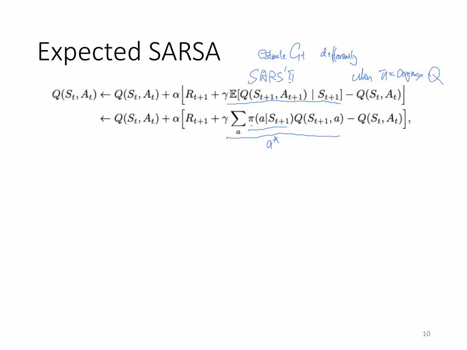
Consider the learning algorithm that is just like Q-learning except that instead of the maximum overnext state–action pairs it uses the expected value, taking into account how likely each action is underthe current policy. That is, consider the algorithm with the update rule

Q(St, At) Q(St, At) + ↵hRt+1 + �E[Q(St+1, At+1) | St+1]�Q(St, At)

i

Q(St, At) + ↵hRt+1 + �

X

a

⇡(a|St+1)Q(St+1, a)�Q(St, At)i, (6.9)

but that otherwise follows the schema of Q-learning. Given the next state, St+1, this algorithm movesdeterministically in the same direction as Sarsa moves in expectation, and accordingly it is calledExpected Sarsa. Its backup diagram is shown on the right in Figure 6.5.

Expected Sarsa is more complex computationally than Sarsa but, in return, it eliminates the variancedue to the random selection of At+1. Given the same amount of experience we might expect it toperform slightly better than Sarsa, and indeed it generally does. Figure 6.6 shows summary resultson the cli↵-walking task with Expected Sarsa compared to Sarsa and Q-learning. Expected Sarsaretains the significant advantage of Sarsa over Q-learning on this problem. In addition, Expected Sarsa

We then present results on two versions of the windygrid world problem, one with a deterministic environmentand one with a stochastic environment. We do so in orderto evaluate the influence of environment stochasticity onthe performance difference between Expected Sarsa andSarsa and confirm the first part of Hypothesis 2. We thenpresent results for different amounts of policy stochasticityto confirm the second part of Hypothesis 2. For completeness,we also show the performance of Q-learning on this problem.Finally, we present results in other domains verifying theadvantages of Expected Sarsa in a broader setting. All resultspresented below are averaged over numerous independenttrials such that the standard error becomes negligible.

A. Cliff Walking

We begin by testing Hypothesis 1 using the cliff walkingtask, an undiscounted, episodic navigation task in which theagent has to find its way from start to goal in a deterministicgrid world. Along the edge of the grid world is a cliff (seeFigure 1). The agent can take any of four movement actions:up, down, left and right, each of which moves the agent onesquare in the corresponding direction. Each step results in areward of -1, except when the agent steps into the cliff area,which results in a reward of -100 and an immediate returnto the start state. The episode ends upon reaching the goalstate.

S G

Fig. 1. The cliff walking task. The agent has to move from the start [S]to the goal [G], while avoiding stepping into the cliff (grey area).

We evaluated the performance over the first n episodes asa function of the learning rate ↵ using an ✏-greedy policywith ✏ = 0.1. Figure 2 shows the result for n = 100 andn = 100, 000. We averaged the results over 50,000 runs and10 runs, respectively.

Discussion. Expected Sarsa outperforms Q-learning andSarsa for all learning rate values, confirming Hypothesis 1and providing some evidence for Hypothesis 2. The optimal↵ value of Expected Sarsa for n = 100 is 1, while forSarsa it is lower, as expected for a deterministic problem.That the optimal value of Q-learning is also lower than 1 issurprising, since Q-learning also has no stochasticity in itsupdates in a deterministic environment. Our explanation isthat Q-learning first learns policies that are sub-optimal inthe greedy sense, i.e. walking towards the goal with a detourfurther from the cliff. Q-learning iteratively optimizes theseearly policies, resulting in a path more closely along the cliff.However, although this path is better in the off-line sense, interms of on-line performance it is worse. A large value of↵ ensures the goal is reached quickly, but a value somewhatlower than 1 ensures that the agent does not try to walk right

on the edge of the cliff immediately, resulting in a slightlybetter on-line performance.

For n = 100, 000, the average return is equal for all↵ values in case of Expected Sarsa and Q-learning. Thisindicates that the algorithms have converged long before theend of the run for all ↵ values, since we do not see anyeffect of the initial learning phase. For Sarsa the performancecomes close to the performance of Expected Sarsa only for↵ = 0.1, while for large ↵, the performance for n = 100, 000even drops below the performance for n = 100. The reasonis that for large values of ↵ the Q values of Sarsa diverge.Although the policy is still improved over the initial randompolicy during the early stages of learning, divergence causesthe policy to get worse in the long run.

0.1 0.2 0.3 0.4 0.5 0.6 0.7 0.8 0.9 1−160

−140

−120

−100

−80

−60

−40

−20

0

alpha

aver

age

retu

rn

n = 100, Sarsan = 100, Q−learningn = 100, Expected Sarsan = 1E5, Sarsan = 1E5, Q−learningn = 1E5, Expected Sarsa

Fig. 2. Average return on the cliff walking task over the first n episodesfor n = 100 and n = 100, 000 using an �-greedy policy with � = 0.1. Thebig dots indicate the maximal values.

B. Windy Grid WorldWe turn to the windy grid world task to further test Hy-

pothesis 2. The windy grid world task is another navigationtask, where the agent has to find its way from start to goal.The grid has a height of 7 and a width of 10 squares. Thereis a wind blowing in the ’up’ direction in the middle part ofthe grid, with a strength of 1 or 2 depending on the column.Figure 3 shows the grid world with a number below eachcolumn indicating the wind strength. Again, the agent canchoose between four movement actions: up, down, left andright, each resulting in a reward of -1. The result of an actionis a movement of 1 square in the corresponding direction plusan additional movement in the ’up’ direction, correspondingwith the wind strength. For example, when the agent is inthe square right of the goal and takes a ’left’ action, it endsup in the square just above the goal.

1) Deterministic Environment: We first consider a de-terministic environment. As in the cliff walking task, weuse an ✏-greedy policy with ✏ = 0.1. Figure 4 shows theperformance as a function of the learning rate ↵ over thefirst n episodes for n = 100 and n = 100, 000. For n = 100

Expected Sarsa

SarsaQ-learning

Asymptotic Performance

Interim Performance

Q-learning

Sum of rewardsper episode

↵10.1 0.2 0.4 0.6 0.80.3 0.5 0.7 0.9

0

-40

-80

-120

Figure 6.6: Interim and asymptotic performance of TD control methods on the cli↵-walking task as a functionof ↵. All algorithms used an "-greedy policy with " = 0.1. Asymptotic performance is an average over 100,000episodes whereas interim performance is an average over the first 100 episodes. These data are averages of over50,000 and 10 runs for the interim and asymptotic cases respectively. The solid circles mark the best interimperformance of each method. Adapted from van Seijen et al. (2009).

Bias in Q-learning and double Q-learning• Q-learning updates

• Double-Q-learning updates• Keep track of two Q function estimates• Toss a coin, if “head”:

• If “tail”: update Q2

12

6.7. MAXIMIZATION BIAS AND DOUBLE LEARNING 111

many possible actions all of which cause immediate termination with a reward drawn from a normaldistribution with mean �0.1 and variance 1.0. Thus, the expected return for any trajectory startingwith left is �0.1, and thus taking left in state A is always a mistake. Nevertheless, our control methodsmay favor left because of maximization bias making B appear to have a positive value. Figure 6.7 showsthat Q-learning with "-greedy action selection initially learns to strongly favor the left action on thisexample. Even at asymptote, Q-learning takes the left action about 5% more often than is optimal atour parameter settings (" = 0.1, ↵ = 0.1, and � = 1).

Are there algorithms that avoid maximization bias? To start, consider a bandit case in which we havenoisy estimates of the value of each of many actions, obtained as sample averages of the rewards receivedon all the plays with each action. As we discussed above, there will be a positive maximization bias ifwe use the maximum of the estimates as an estimate of the maximum of the true values. One way toview the problem is that it is due to using the same samples (plays) both to determine the maximizingaction and to estimate its value. Suppose we divided the plays in two sets and used them to learn twoindependent estimates, call them Q1(a) and Q2(a), each an estimate of the true value q(a), for all a 2 A.We could then use one estimate, say Q1, to determine the maximizing action A⇤ = argmax

aQ1(a), and

the other, Q2, to provide the estimate of its value, Q2(A⇤) = Q2(argmaxaQ1(a)). This estimate will

then be unbiased in the sense that E[Q2(A⇤)] = q(A⇤). We can also repeat the process with the role ofthe two estimates reversed to yield a second unbiased estimate Q1(argmax

aQ2(a)). This is the idea of

double learning. Note that although we learn two estimates, only one estimate is updated on each play;double learning doubles the memory requirements, but does not increase the amount of computationper step.

The idea of double learning extends naturally to algorithms for full MDPs. For example, the doublelearning algorithm analogous to Q-learning, called Double Q-learning, divides the time steps in two,perhaps by flipping a coin on each step. If the coin comes up heads, the update is

Q1(St, At) Q1(St, At) + ↵hRt+1 + �Q2

�St+1, argmax

a

Q1(St+1, a)��Q1(St, At)

i. (6.10)

If the coin comes up tails, then the same update is done with Q1 and Q2 switched, so that Q2 is updated.The two approximate value functions are treated completely symmetrically. The behavior policy canuse both action-value estimates. For example, an "-greedy policy for Double Q-learning could be basedon the average (or sum) of the two action-value estimates. A complete algorithm for Double Q-learningis given below. This is the algorithm used to produce the results in Figure 6.7. In that example, doublelearning seems to eliminate the harm caused by maximization bias. Of course there are also doubleversions of Sarsa and Expected Sarsa.

Double Q-learning

Initialize Q1(s, a) and Q2(s, a), for all s 2 S, a 2 A(s), arbitrarilyInitialize Q1(terminal-state, ·) = Q2(terminal-state, ·) = 0Repeat (for each episode):

Initialize S

Repeat (for each step of episode):Choose A from S using policy derived from Q1 and Q2 (e.g., "-greedy in Q1 + Q2)Take action A, observe R, S

0

With 0.5 probabilility:

Q1(S, A) Q1(S, A) + ↵

⇣R + �Q2

�S

0, argmaxa Q1(S

0, a)

��Q1(S, A)

⌘

else:

Q2(S, A) Q2(S, A) + ↵

⇣R + �Q1

�S

0, argmaxa Q2(S

0, a)

��Q2(S, A)

⌘

S S0

until S is terminal

6.5. Q-LEARNING: OFF-POLICY TD CONTROL 107

The graph in Figure 6.3 shows the results of applying "-greedy Sarsa to this task, with " = 0.1,↵ = 0.5, and the initial values Q(s, a) = 0 for all s, a. The increasing slope of the graph showsthat the goal is reached more and more quickly over time. By 8000 time steps, the greedy policywas long since optimal (a trajectory from it is shown inset); continued "-greedy exploration kept theaverage episode length at about 17 steps, two more than the minimum of 15. Note that Monte Carlomethods cannot easily be used on this task because termination is not guaranteed for all policies.If a policy was ever found that caused the agent to stay in the same state, then the next episodewould never end. Step-by-step learning methods such as Sarsa do not have this problem becausethey quickly learn during the episode that such policies are poor, and switch to something else.

Exercise 6.9: Windy Gridworld with King’s Moves Re-solve the windy gridworld task assuming eightpossible actions, including the diagonal moves, rather than the usual four. How much better can you dowith the extra actions? Can you do even better by including a ninth action that causes no movementat all other than that caused by the wind? ⇤Exercise 6.10: Stochastic Wind Re-solve the windy gridworld task with King’s moves, assumingthat the e↵ect of the wind, if there is any, is stochastic, sometimes varying by 1 from the mean valuesgiven for each column. That is, a third of the time you move exactly according to these values, as inthe previous exercise, but also a third of the time you move one cell above that, and another third ofthe time you move one cell below that. For example, if you are one cell to the right of the goal andyou move left, then one-third of the time you move one cell above the goal, one-third of the time youmove two cells above the goal, and one-third of the time you move to the goal. ⇤

6.5 Q-learning: O↵-policy TD Control

One of the early breakthroughs in reinforcement learning was the development of an o↵-policy TDcontrol algorithm known as Q-learning (Watkins, 1989), defined by

Q(St, At) Q(St, At) + ↵hRt+1 + � max

a

Q(St+1, a)�Q(St, At)i. (6.8)

In this case, the learned action-value function, Q, directly approximates q⇤, the optimal action-valuefunction, independent of the policy being followed. This dramatically simplifies the analysis of thealgorithm and enabled early convergence proofs. The policy still has an e↵ect in that it determineswhich state–action pairs are visited and updated. However, all that is required for correct convergenceis that all pairs continue to be updated. As we observed in Chapter 5, this is a minimal requirementin the sense that any method guaranteed to find optimal behavior in the general case must require it.Under this assumption and a variant of the usual stochastic approximation conditions on the sequenceof step-size parameters, Q has been shown to converge with probability 1 to q⇤.

Q-learning (o↵-policy TD control) for estimating ⇡ ⇡ ⇡⇤

Initialize Q(s, a), for all s 2 S, a 2 A(s), arbitrarily, and Q(terminal-state, ·) = 0Repeat (for each episode):

Initialize S

Repeat (for each step of episode):Choose A from S using policy derived from Q (e.g., ✏-greedy)Take action A, observe R, S

0

Q(S, A) Q(S, A) + ↵⇥R + � maxa Q(S0

, a)�Q(S, A)⇤

S S0

until S is terminal

The problem of large state-spaceis still there• We need to represent and learn SA parameters in Q-learning and SARSA.

• S is often large• 9-puzzle, Tic-Tac-Toe: 9! = 362,800, S^2 = 1.3*10^11• PACMAN with 20 by 20 grid. S = O(2^400), S^2 = O(2^800)

• O(S) is not acceptable in some cases.

• Need to think of ways to “generalize”/shareinformation across states.

13

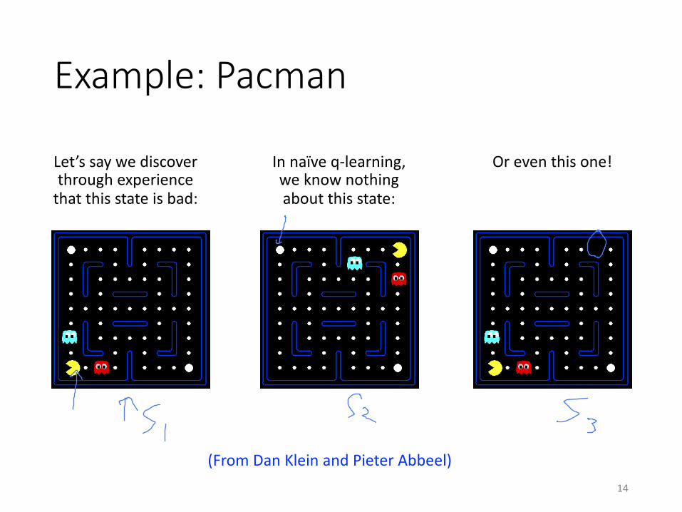
Example: Pacman

Let’s say we discover through experience

that this state is bad:

In naïve q-learning, we know nothing about this state:

Or even this one!

(From Dan Klein and Pieter Abbeel)14

Video of Demo Q-Learning Pacman – Tiny – Watch All

15

Video of Demo Q-Learning Pacman – Tiny – Silent Train

16

Video of Demo Q-Learning Pacman – Tricky –Watch All

17

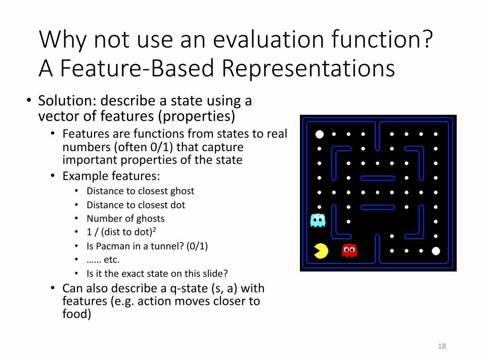
Why not use an evaluation function?A Feature-Based Representations

• Solution: describe a state using a vector of features (properties)• Features are functions from states to real

numbers (often 0/1) that capture important properties of the state

• Example features:• Distance to closest ghost• Distance to closest dot• Number of ghosts• 1 / (dist to dot)2

• Is Pacman in a tunnel? (0/1)• …… etc.• Is it the exact state on this slide?

• Can also describe a q-state (s, a) with features (e.g. action moves closer to food)

18

Linear Value Functions

• Using a feature representation, we can write a q function (or value function) for any state using a few weights:

• Vw(s) = w1f1(s) + w2f2(s) + … + wnfn(s)

• Qw(s,a) = w1f1(s,a) + w2f2(s,a) + … + wnfn(s,a)

• Advantage: our experience is summed up in a few powerful numbers

• Disadvantage: states may share features but actually be very different in value!

19

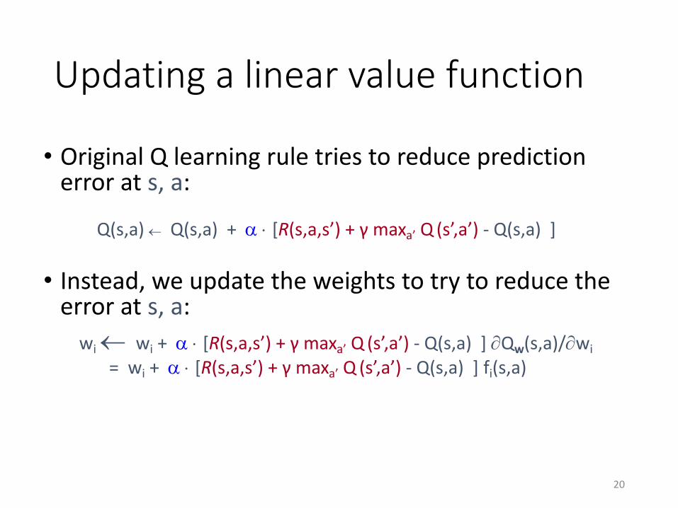
Updating a linear value function

• Original Q learning rule tries to reduce prediction error at s, a:

Q(s,a) ¬ Q(s,a) + a × [R(s,a,s’) + γ maxa’ Q (s’,a’) - Q(s,a) ]

• Instead, we update the weights to try to reduce the error at s, a:

wi¬ wi + a × [R(s,a,s’) + γ maxa’ Q (s’,a’) - Q(s,a) ] ¶Qw(s,a)/¶wi= wi + a × [R(s,a,s’) + γ maxa’ Q (s’,a’) - Q(s,a) ] fi(s,a)

20

Updating a linear value function

• Original Q learning rule tries to reduce prediction error at s, a:

Q(s,a) ¬ Q(s,a) + a × [R(s,a,s’) + γ maxa’ Q (s’,a’) - Q(s,a) ]

• Instead, we update the weights to try to reduce the error at s, a:wi¬ wi + a × [R(s,a,s’) + γ maxa’ Q (s’,a’) - Q(s,a) ] ¶Qw(s,a)/¶wi

= wi + a × [R(s,a,s’) + γ maxa’ Q (s’,a’) - Q(s,a) ] fi(s,a)

• Qualitative justification:• Pleasant surprise: increase weights on positive features, decrease on negative

ones• Unpleasant surprise: decrease weights on positive features, increase on negative

ones

21

PACMAN Q-Learning (Linear functionapprox.)

22

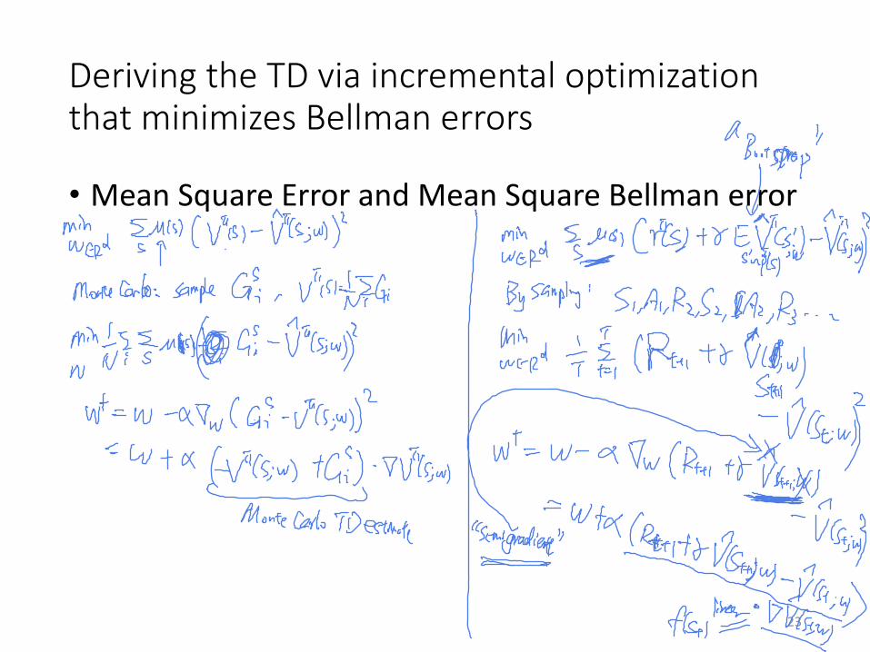
Deriving the TD via incremental optimization that minimizes Bellman errors

• Mean Square Error and Mean Square Bellman error

23

How do we make sense of thesemi-gradient method?

24

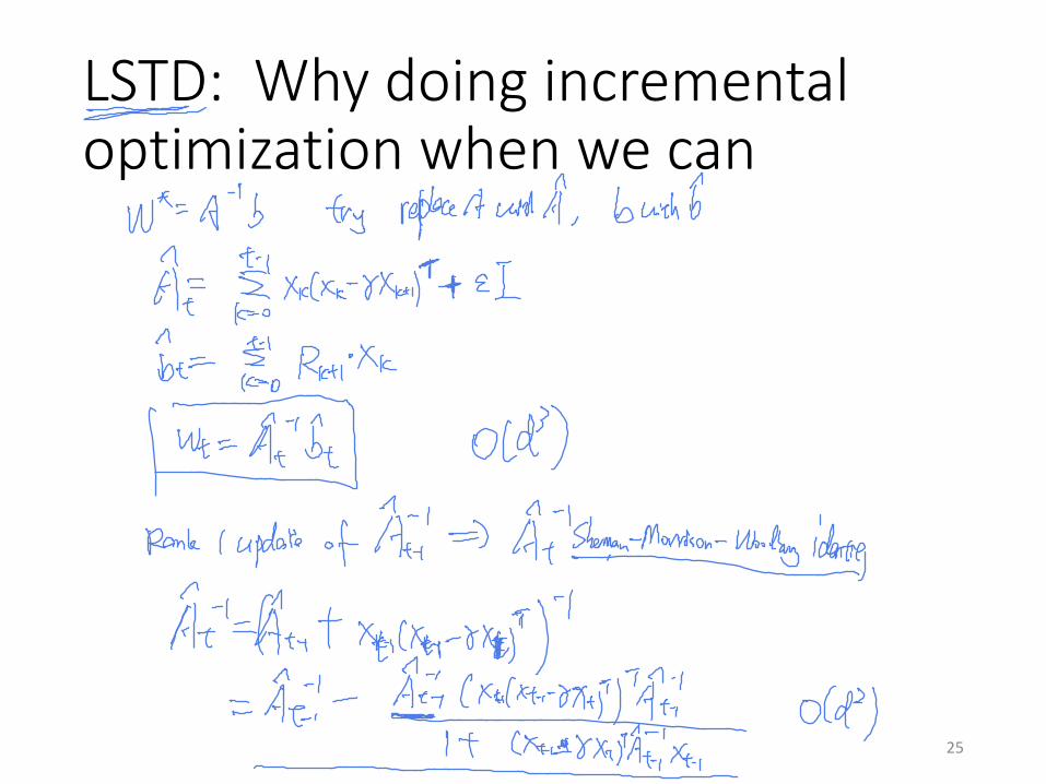
LSTD: Why doing incremental optimization when we can

25

So far, in RL algorithms

• Model-based approaches• Estimate the MDP parameters.• Then use policy-iterations, value iterations.

• Monte Carlo methods:• estimating the rewards by empirical averages

• Temporal Difference methods:• Combine Monte Carlo methods with Dynamic Programming

• Linear function approximation in Q-learning• Similar to SGD• Learning heuristic function

26*Question: What is the policy class Π of interest in these methods?

Remainder of the lecture

• Policy gradients methods

• Policy gradient theorem

• Extensions

27

So far we talked about value function approximation, and an induced policy class.

• We can directly work with a parametric policy class.

• Examples:

28

Optimize policy using SGD

29

How to estimate the gradient?

• Policy gradient theorem:

30

Proof of Policy Gradient Theorem

31

Proof of Policy Gradient Theorem

32

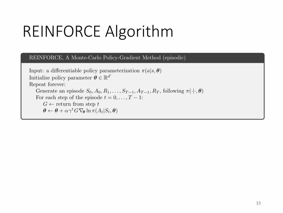
REINFORCE Algorithm

33

13.3. REINFORCE: MONTE CARLO POLICY GRADIENT 271

REINFORCE, A Monte-Carlo Policy-Gradient Method (episodic)

Input: a di↵erentiable policy parameterization ⇡(a|s, ✓)Initialize policy parameter ✓ 2 Rd

0

Repeat forever:Generate an episode S0, A0, R1, . . . , ST�1, AT�1, RT , following ⇡(·|·, ✓)For each step of the episode t = 0, . . . , T � 1:

G return from step t✓ ✓ + ↵�tGr✓ ln ⇡(At|St, ✓)

Figure 13.1 shows the performance of REINFORCE, averaged over 100 runs, on the gridworld fromExample 13.1.

The vector r✓⇡(At|St,✓t)⇡(At|St,✓t)

in the REINFORCE update is the only place the policy parameterizationappears in the algorithm. This vector has been given several names and notations in the literature;we will refer to it simply as the eligibility vector. The eligibility vector is often written in the compactform r✓ ln ⇡(At|St, ✓t), using the identity r ln x = rx

x. This form is used in all the boxed pseudocode

in this chapter. In earlier examples in this chapter we considered exponential softmax policies (13.2)with linear action preferences (13.3). For this parameterization, the eligibility vector is

r✓ ln ⇡(a|s, ✓) = x(s, a)�X

b

⇡(b|s, ✓)x(s, b). (13.7)

As a stochastic gradient method, REINFORCE has good theoretical convergence properties. Byconstruction, the expected update over an episode is in the same direction as the performance gradient.2

This assures an improvement in expected performance for su�ciently small ↵, and convergence to a

2Technically, this is only true if each episode’s updates are done o↵-line, meaning they are accumulated on the side

during the episode and only used to change ✓ by their sum at the episode’s end. However, this would probably be a

worse algorithm in practice, and its desirable theoretical properties would probably be shared by the algorithm as given

(although this has not been proved).

↵ = 2�13

↵ = 2�12

Episode10008006004002001

-80

-90

-60

-40

-20

-10

Total rewardper episode

G0

v⇤(s0)

↵ = 2�14

Figure 13.1: REINFORCE on the short-corridor gridworld (Example 13.1). With a good step size, the totalreward per episode approaches the optimal value of the start state.

Actor-Critic algorithm

• REINFORCE with a given baseline

• Actor-Critic: Learn the baseline and use the baseline for “bootstrapping”

34

Next lecture

• Wrap up RL algorithms

• Exploration: Multi-armed bandits

35