CS 445 / 645 Introduction to Computer Graphics Lecture 19 Texture Maps Lecture 19 Texture Maps.
Upload
anastasia-mosleyCategory
view
31download
4description

CS 445 / 645Introduction to Computer Graphics
Lecture 23Lecture 23
BBézier Curvesézier Curves
Lecture 23Lecture 23
BBézier Curvesézier Curves

Splines - History
Draftsman use ‘ducks’ and Draftsman use ‘ducks’ and strips of wood (splines) to strips of wood (splines) to draw curvesdraw curves
Wood splines have second-Wood splines have second-order continuityorder continuity
And pass through the And pass through the control pointscontrol points
Draftsman use ‘ducks’ and Draftsman use ‘ducks’ and strips of wood (splines) to strips of wood (splines) to draw curvesdraw curves
Wood splines have second-Wood splines have second-order continuityorder continuity
And pass through the And pass through the control pointscontrol points
A Duck (weight)
Ducks trace out curve

Representations of Curves
Problems with series of points used to model a curveProblems with series of points used to model a curve
• Piecewise linear - Does not accurately model a smooth linePiecewise linear - Does not accurately model a smooth line
• It’s tediousIt’s tedious
• Expensive to manipulate curve because all points must be repositionedExpensive to manipulate curve because all points must be repositioned
Instead, model curve as piecewise-polynomialInstead, model curve as piecewise-polynomial
• x = x(t), y = y(t), z = z(t) x = x(t), y = y(t), z = z(t)
– where x(), y(), z() are polynomials where x(), y(), z() are polynomials

Specifying Curves (hyperlink)
Control PointsControl Points
• A set of points that influence the A set of points that influence the curve’s shapecurve’s shape
KnotsKnots
• Control points that lie on the curveControl points that lie on the curve
Interpolating SplinesInterpolating Splines
• Curves that pass through the control Curves that pass through the control points (knots)points (knots)
Approximating SplinesApproximating Splines
• Control points merely influence shapeControl points merely influence shape

Parametric Curves
Very flexible representationVery flexible representation
They are not required to be functionsThey are not required to be functions
• They can be multivalued with respect to any dimensionThey can be multivalued with respect to any dimension
Very flexible representationVery flexible representation
They are not required to be functionsThey are not required to be functions
• They can be multivalued with respect to any dimensionThey can be multivalued with respect to any dimension

Cubic Polynomials
x(t) = ax(t) = axxtt33 + b + bxxtt22 + c + cxxt + dt + dxx
• Similarly for y(t) and z(t)Similarly for y(t) and z(t)
Let t: (0 <= t <= 1)Let t: (0 <= t <= 1)
Let T = [tLet T = [t33 t t22 t 1] t 1]
Coefficient Matrix CCoefficient Matrix C
Curve: Q(t) = T*CCurve: Q(t) = T*C
x(t) = ax(t) = axxtt33 + b + bxxtt22 + c + cxxt + dt + dxx
• Similarly for y(t) and z(t)Similarly for y(t) and z(t)
Let t: (0 <= t <= 1)Let t: (0 <= t <= 1)
Let T = [tLet T = [t33 t t22 t 1] t 1]
Coefficient Matrix CCoefficient Matrix C
Curve: Q(t) = T*CCurve: Q(t) = T*C
[ ]
⎥⎥⎥⎥⎥⎥
⎦
⎤
⎢⎢⎢⎢⎢⎢
⎣
⎡
∗
z
z
y
y
x
x
zyx
zyx
d
c
d
c
d
c
bbb
aaa
ttt 123

Parametric Curves
How do we find the tangent to a curve?How do we find the tangent to a curve?
• If f(x) = xIf f(x) = x22 – 4 – 4
– tangent at (x=3) is f’(x) = 2 (x) – 4 = 2 (3) - 4tangent at (x=3) is f’(x) = 2 (x) – 4 = 2 (3) - 4
How do we find the tangent to a curve?How do we find the tangent to a curve?
• If f(x) = xIf f(x) = x22 – 4 – 4
– tangent at (x=3) is f’(x) = 2 (x) – 4 = 2 (3) - 4tangent at (x=3) is f’(x) = 2 (x) – 4 = 2 (3) - 4
Derivative of Q(t) is the tangent vector at t:Derivative of Q(t) is the tangent vector at t:
• d/dt Q(t) = Q’(t) = d/dt T * C = [3td/dt Q(t) = Q’(t) = d/dt T * C = [3t22 2t 1 0] * C 2t 1 0] * C
Derivative of Q(t) is the tangent vector at t:Derivative of Q(t) is the tangent vector at t:
• d/dt Q(t) = Q’(t) = d/dt T * C = [3td/dt Q(t) = Q’(t) = d/dt T * C = [3t22 2t 1 0] * C 2t 1 0] * C

Piecewise Curve Segments
One curve constructed by connecting many smaller segments end-One curve constructed by connecting many smaller segments end-to-endto-end
Continuity describes the jointContinuity describes the joint
• CC11 is tangent continuity (velocity) is tangent continuity (velocity)
• CC22 is 2 is 2ndnd derivative continuity (acceleration) derivative continuity (acceleration)

Continuity of Curves
If direction (but not necessarily magnitude) of tangent If direction (but not necessarily magnitude) of tangent matchesmatches• GG11 geometric continuity geometric continuity
• The tangent value at the end of one curve is proportional to the The tangent value at the end of one curve is proportional to the tangent value of the beginning of the next curvetangent value of the beginning of the next curve
Matching direction and magnitude of dMatching direction and magnitude of dnn / dt / dtnn
– CCnn continous continous

Parametric Cubic Curves
In order to assure CIn order to assure C22 continuity, curves must be of continuity, curves must be of
at least degree 3at least degree 3
Here is the parametric definition of a cubic Here is the parametric definition of a cubic (degree 3) spline in two dimensions(degree 3) spline in two dimensions
How do we extend it to three dimensions?How do we extend it to three dimensions?

Parametric Cubic Splines
Can represent this as a matrix tooCan represent this as a matrix tooCan represent this as a matrix tooCan represent this as a matrix too

Coefficients
So how do we select the coefficients?So how do we select the coefficients?
• [a[axx b bxx c cxx d dxx] and [a] and [ayy b byy c cyy d dyy] must satisfy the constraints ] must satisfy the constraints
defined by the knots and the continuity conditionsdefined by the knots and the continuity conditions
So how do we select the coefficients?So how do we select the coefficients?
• [a[axx b bxx c cxx d dxx] and [a] and [ayy b byy c cyy d dyy] must satisfy the constraints ] must satisfy the constraints
defined by the knots and the continuity conditionsdefined by the knots and the continuity conditions

Parametric Curves
Difficult to conceptualize curve as Difficult to conceptualize curve as x(t) = ax(t) = axxtt33 + b + bxxtt22 + c + cxxt + dt + dxx
(artists don’t think in terms of coefficients of cubics)(artists don’t think in terms of coefficients of cubics)
Instead, define curve as weighted combination of 4 well-defined Instead, define curve as weighted combination of 4 well-defined cubic polynomialscubic polynomials(wait a second! Artists don’t think this way either!)(wait a second! Artists don’t think this way either!)
Each curve type defines different cubic polynomials and weighting Each curve type defines different cubic polynomials and weighting schemesschemes

Parametric Curves
HermiteHermite – two endpoints and two endpoint tangent – two endpoints and two endpoint tangent vectorsvectors
BezierBezier - two endpoints and two other points that define - two endpoints and two other points that define the endpoint tangent vectorsthe endpoint tangent vectors
SplinesSplines – four control points – four control points • C1 and C2 continuity at the join pointsC1 and C2 continuity at the join points
• Come close to their control points, but not guaranteed to touch themCome close to their control points, but not guaranteed to touch them
Examples of SplinesExamples of Splines

Hermite Cubic Splines
An example of knot and continuity constraintsAn example of knot and continuity constraintsAn example of knot and continuity constraintsAn example of knot and continuity constraints

Hermite Cubic Splines
One cubic curve for each dimensionOne cubic curve for each dimension
A curve constrained to x/y-plane has two curves:A curve constrained to x/y-plane has two curves:
One cubic curve for each dimensionOne cubic curve for each dimension
A curve constrained to x/y-plane has two curves:A curve constrained to x/y-plane has two curves:
[ ]⎥⎥⎥⎥
⎦
⎤
⎢⎢⎢⎢
⎣
⎡
=
+++=
d
c
b
a
ttt
dctbtattf x
1
)(
23
23
[ ]⎥⎥⎥⎥
⎦
⎤
⎢⎢⎢⎢
⎣
⎡
=
+++=
h
g
f
e
ttt
hgtftettf y
1
)(
23
23

Hermite Cubic Splines
A 2-D Hermite Cubic Spline is defined by eight A 2-D Hermite Cubic Spline is defined by eight parameters: a, b, c, d, e, f, g, hparameters: a, b, c, d, e, f, g, h
How do we convert the intuitive endpoint constraints into How do we convert the intuitive endpoint constraints into these (relatively) unintuitive eight parameters?these (relatively) unintuitive eight parameters?
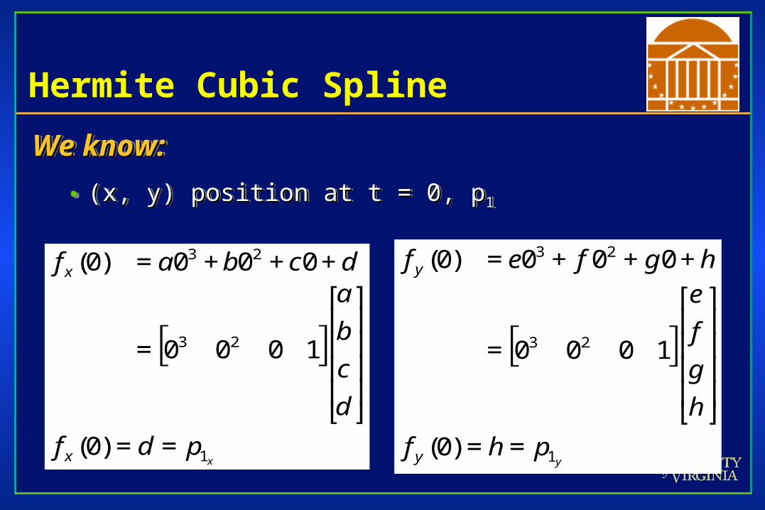
We know:We know:• (x, y) position at t = 0, p(x, y) position at t = 0, p11
• (x, y) position at t = 1, p(x, y) position at t = 1, p22
• (x, y) derivative at t = 0, dp/dt(x, y) derivative at t = 0, dp/dt
• (x, y) derivative at t = 1, dp/dt(x, y) derivative at t = 1, dp/dt
A 2-D Hermite Cubic Spline is defined by eight A 2-D Hermite Cubic Spline is defined by eight parameters: a, b, c, d, e, f, g, hparameters: a, b, c, d, e, f, g, h
How do we convert the intuitive endpoint constraints into How do we convert the intuitive endpoint constraints into these (relatively) unintuitive eight parameters?these (relatively) unintuitive eight parameters?
We know:We know:• (x, y) position at t = 0, p(x, y) position at t = 0, p11
• (x, y) position at t = 1, p(x, y) position at t = 1, p22
• (x, y) derivative at t = 0, dp/dt(x, y) derivative at t = 0, dp/dt
• (x, y) derivative at t = 1, dp/dt(x, y) derivative at t = 1, dp/dt
Hermite Cubic Spline
We know:We know:
• (x, y) position at t = 0, p(x, y) position at t = 0, p11
We know:We know:
• (x, y) position at t = 0, p(x, y) position at t = 0, p11
[ ]
xpdf
d
c
b
adcbaf
x
x
1
23
23
)0(
1000
000)0(
==
⎥⎥⎥⎥
⎦
⎤
⎢⎢⎢⎢
⎣
⎡
=
+++=
[ ]
yphf
h
g
f
ehgfef
y
y
1
23
23
)0(
1000
000)0(
==
⎥⎥⎥⎥
⎦
⎤
⎢⎢⎢⎢
⎣
⎡
=
+++=

Hermite Cubic Spline
We know:We know:
• (x, y) position at t = 1, p(x, y) position at t = 1, p22
We know:We know:
• (x, y) position at t = 1, p(x, y) position at t = 1, p22
[ ]
xpdcbaf
d
c
b
adcbaf
x
x
2
23
23
)1(
1111
111)1(
=+++=
⎥⎥⎥⎥
⎦
⎤
⎢⎢⎢⎢
⎣
⎡
=
+++=
[ ]
yphgfef
h
g
f
ehgfef
y
y
2
23
23
)1(
1111
111)1(
=+++=
⎥⎥⎥⎥
⎦
⎤
⎢⎢⎢⎢
⎣
⎡
=
+++=

Hermite Cubic Splines
So far we have four equations, but we have eight So far we have four equations, but we have eight unknownsunknowns
Use the derivativesUse the derivatives
So far we have four equations, but we have eight So far we have four equations, but we have eight unknownsunknowns
Use the derivativesUse the derivatives
[ ]⎥⎥⎥⎥
⎦
⎤
⎢⎢⎢⎢
⎣
⎡
=′
++=′
+++=
d
c
b
a
tttf
cbtattf
dctbtattf
x
x
x
0123)(
23)(
)(
2
2
23
[ ]⎥⎥⎥⎥
⎦
⎤
⎢⎢⎢⎢
⎣
⎡
=′
++=′
+++=
h
g
f
e
tttf
gftettf
hgtftettf
y
y
y
0123)(
23)(
)(
2
2
23

Hermite Cubic Spline
We know:We know:
• (x, y) derivative at t = 0, dp/dt(x, y) derivative at t = 0, dp/dt
We know:We know:
• (x, y) derivative at t = 0, dp/dt(x, y) derivative at t = 0, dp/dt
[ ]
dtdp
cf
d
c
b
acbaf
xx
x
1
2
2
)0(
010203
0203)0(
==′
⎥⎥⎥⎥
⎦
⎤
⎢⎢⎢⎢
⎣
⎡
⋅⋅=
++=′
[ ]
dtdp
gf
h
g
f
egfef
y
y
y
1
2
2
)0(
010203
0203)0(
==′
⎥⎥⎥⎥
⎦
⎤
⎢⎢⎢⎢
⎣
⎡
⋅⋅=
++=′

Hermite Cubic Spline
We know:We know:
• (x, y) derivative at t = 1, dp/dt(x, y) derivative at t = 1, dp/dt
We know:We know:
• (x, y) derivative at t = 1, dp/dt(x, y) derivative at t = 1, dp/dt
[ ]
dtdp
cbaf
d
c
b
acbaf
xx
x
1
2
2
23)1(
011213
1213)1(
=++=′
⎥⎥⎥⎥
⎦
⎤
⎢⎢⎢⎢
⎣
⎡
⋅⋅=
++=′
[ ]
dtdp
gfef
h
g
f
egfef
y
y
y
1
2
2
23)1(
011213
1213)1(
=++=′
⎥⎥⎥⎥
⎦
⎤
⎢⎢⎢⎢
⎣
⎡
⋅⋅=
++=′

Hermite Specification
Matrix equation for Hermite CurveMatrix equation for Hermite CurveMatrix equation for Hermite CurveMatrix equation for Hermite Curve
t = 0
t = 1
t = 0
t = 1
t3 t2 t1 t0
p1
p2
r p1
r p2

Solve Hermite Matrix

Spline and Geometry Matrices
MHermite GHermite

Resulting Hermite Spline Equation

Demonstration
HermiteHermite

Sample Hermite Curves

Blending Functions
By multiplying first two matrices in lower-left By multiplying first two matrices in lower-left equation, you have four functions of ‘t’ that equation, you have four functions of ‘t’ that blend the four control parametersblend the four control parameters
These are blendingThese are blendingfunctionsfunctions

Hermite Blending Functions
If you plot the If you plot the blending blending functions on functions on the parameter the parameter ‘t’‘t’
If you plot the If you plot the blending blending functions on functions on the parameter the parameter ‘t’‘t’

Hermite Blending Functions
Remember, eachRemember, eachblending functionblending functionreflects influencereflects influenceof Pof P11, P, P22, , PP11, , PP22
on spline’s shapeon spline’s shape
Remember, eachRemember, eachblending functionblending functionreflects influencereflects influenceof Pof P11, P, P22, , PP11, , PP22
on spline’s shapeon spline’s shape

Bézier Curves
Similar to Hermite, but more intuitive definition of Similar to Hermite, but more intuitive definition of endpoint derivativesendpoint derivatives
Four control points, two of which are knotsFour control points, two of which are knots
Similar to Hermite, but more intuitive definition of Similar to Hermite, but more intuitive definition of endpoint derivativesendpoint derivatives
Four control points, two of which are knotsFour control points, two of which are knots

Bézier Curves
The derivative values of the Bezier Curve at the The derivative values of the Bezier Curve at the knots are dependent on the adjacent pointsknots are dependent on the adjacent points
The scalar 3 was selected just for this curve The scalar 3 was selected just for this curve
The derivative values of the Bezier Curve at the The derivative values of the Bezier Curve at the knots are dependent on the adjacent pointsknots are dependent on the adjacent points
The scalar 3 was selected just for this curve The scalar 3 was selected just for this curve

Bézier vs. Hermite
We can write our Bezier in terms of HermiteWe can write our Bezier in terms of Hermite
• Note this is just matrix form of previous equationsNote this is just matrix form of previous equations
We can write our Bezier in terms of HermiteWe can write our Bezier in terms of Hermite
• Note this is just matrix form of previous equationsNote this is just matrix form of previous equations

Bézier vs. Hermite
Now substitute this in for previous HermiteNow substitute this in for previous HermiteNow substitute this in for previous HermiteNow substitute this in for previous Hermite

Bézier Basis and Geometry Matrices
Matrix FormMatrix Form
But why is MBut why is MBezierBezier a good basis matrix? a good basis matrix?
Matrix FormMatrix Form
But why is MBut why is MBezierBezier a good basis matrix? a good basis matrix?

Bézier Blending Functions
Look at the blending Look at the blending functionsfunctions
This family of This family of polynomials is calledpolynomials is calledorder-3 Bernstein order-3 Bernstein PolynomialsPolynomials• C(3, k) tC(3, k) tkk (1-t) (1-t)3-k3-k; 0<= k <= 3; 0<= k <= 3
• They are all positive in interval [0,1]They are all positive in interval [0,1]
• Their sum is equal to 1Their sum is equal to 1

Bézier Blending Functions
Thus, every point on curve is Thus, every point on curve is linear combination of the linear combination of the control pointscontrol points
The weights of the The weights of the combination are all positivecombination are all positive
The sum of the weights is 1The sum of the weights is 1
Therefore, the curve is a Therefore, the curve is a convex combination of the convex combination of the control pointscontrol points

Bézier Curves
Will always remain within bounding region Will always remain within bounding region defined by control pointsdefined by control points
Will always remain within bounding region Will always remain within bounding region defined by control pointsdefined by control points

Bézier Curves
BezierBezierBezierBezier
Why more spline slides?
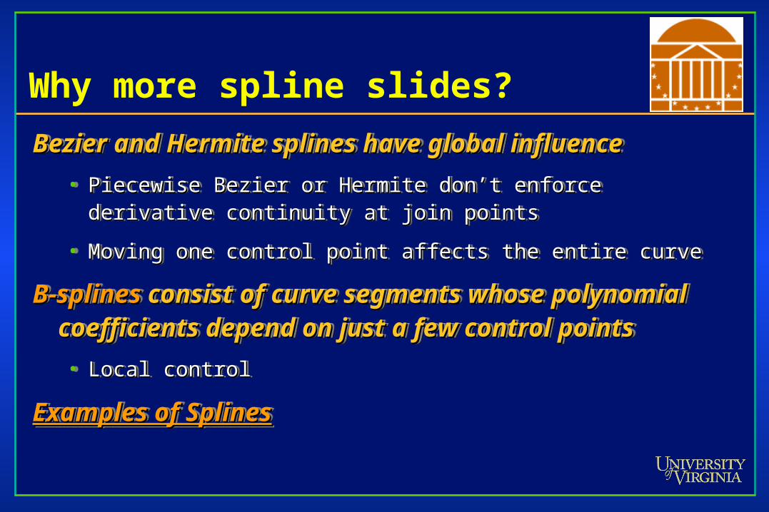
Bezier and Hermite splines have global influenceBezier and Hermite splines have global influence
• Piecewise Bezier or Hermite don’t enforce derivative continuity at join Piecewise Bezier or Hermite don’t enforce derivative continuity at join pointspoints
• Moving one control point affects the entire curveMoving one control point affects the entire curve
B-splinesB-splines consist of curve segments whose polynomial consist of curve segments whose polynomial coefficients depend on just a few control pointscoefficients depend on just a few control points
• Local controlLocal control
Examples of SplinesExamples of Splines

B-Spline Curve
Start with a sequence of control pointsStart with a sequence of control points
Select four from middle of sequence Select four from middle of sequence (p(pi-2i-2, p, pi-1i-1, p, pii, p, pi+1i+1) ) dd
• Bezier and Hermite goes between pBezier and Hermite goes between p i-2i-2 and p and pi+1i+1
• B-Spline doesn’t interpolate (touch) any of them but B-Spline doesn’t interpolate (touch) any of them but approximates the going through papproximates the going through p i-1i-1 and p and pii
pp00pp00 pp44pp44
pp22pp22pp11pp11
pp33pp33
pp55pp55
pp66pp66
QQ33QQ33
QQ44QQ44
QQ55QQ55
QQ66QQ66

Uniform B-Splines
ApproximatingApproximating Splines Splines
Approximates n+1 control pointsApproximates n+1 control points
• PP00, P, P11, …, P, …, Pnn, n , n ¸̧ 3 3
Curve consists of n –2 cubic polynomial segmentsCurve consists of n –2 cubic polynomial segments
• QQ33, Q, Q44, … Q, … Qnn
t varies along B-spline as Qt varies along B-spline as Qii: t: tii <= t < t <= t < ti+1i+1
ttii (i = integer) are (i = integer) are knot pointsknot points that join segment Q that join segment Qi-1i-1 to Q to Qii
Curve is Curve is uniformuniform because knots are spaced at equal intervals of because knots are spaced at equal intervals of parameter,parameter, tt

Uniform B-Splines
First curve segment, QFirst curve segment, Q33, is defined by first four , is defined by first four
control pointscontrol points
Last curve segment, QLast curve segment, Qmm, is defined by last four , is defined by last four
control points, Pcontrol points, Pm-3m-3, P, Pm-2m-2, P, Pm-1m-1, P, Pmm
Each control point affects four curve segmentsEach control point affects four curve segments

B-spline Basis Matrix
Formulate 16 equations to solve the 16 unknownsFormulate 16 equations to solve the 16 unknowns
The 16 equations enforce the CThe 16 equations enforce the C00, C, C11, and C, and C22
continuity between adjoining segments, Qcontinuity between adjoining segments, Q
Formulate 16 equations to solve the 16 unknownsFormulate 16 equations to solve the 16 unknowns
The 16 equations enforce the CThe 16 equations enforce the C00, C, C11, and C, and C22
continuity between adjoining segments, Qcontinuity between adjoining segments, Q
⎥⎥⎥⎥
⎦
⎤
⎢⎢⎢⎢
⎣
⎡
−−
−−
=−
0141
0303
0363
1331
6
1splineBM

B-Spline Basis Matrix
Note the order of the rows in my MNote the order of the rows in my MB-Spline B-Spline is is
different from in the bookdifferent from in the book
• Observe also that the order in which I number the points is Observe also that the order in which I number the points is differentdifferent
• Therefore my matrix aligns with the book’s matrix if you Therefore my matrix aligns with the book’s matrix if you reorder the points, and thus reorder the rows of the matrixreorder the points, and thus reorder the rows of the matrix

B-Spline
Points along B-Spline are computed just as with Points along B-Spline are computed just as with Bezier CurvesBezier Curves
Points along B-Spline are computed just as with Points along B-Spline are computed just as with Bezier CurvesBezier Curves
( ) PUMtQ SplineBi −=
( ) [ ]⎥⎥⎥⎥
⎦
⎤
⎢⎢⎢⎢
⎣
⎡
⎥⎥⎥⎥
⎦
⎤
⎢⎢⎢⎢
⎣
⎡
−−
−−
=
+
+
+
3
2
123
0141
0303
0363
1331
6
11
i
i
i
i
i
p
p
p
p
ttttQ

B-Spline
By far the most popular spline usedBy far the most popular spline used
CC00, C, C11, and C, and C22 continuous continuous
By far the most popular spline usedBy far the most popular spline used
CC00, C, C11, and C, and C22 continuous continuous

B-Spline
Locality of pointsLocality of pointsLocality of pointsLocality of points

Nonuniform, Rational B-Splines(NURBS)
The native geometry element in MayaThe native geometry element in Maya
Models are composed of surfaces defined by Models are composed of surfaces defined by NURBS, not polygonsNURBS, not polygons
NURBS are smoothNURBS are smooth
NURBS require effort to make non-smoothNURBS require effort to make non-smooth

NURBs
To generate three-dimension pointsTo generate three-dimension points
• Four B-Splines are usedFour B-Splines are used
– Three define the x, y, and z positionThree define the x, y, and z position
– One defines a weighting termOne defines a weighting term
• The 3-D point output by a NURB is the x, y, z coordinates The 3-D point output by a NURB is the x, y, z coordinates divided by the weighting term (like homogeneous divided by the weighting term (like homogeneous coordinates)coordinates)

What is a NURB?
Nonuniform:Nonuniform: The amount of parameter, t, that is The amount of parameter, t, that is used to model each curve segment varies used to model each curve segment varies • Nonuniformity permits either CNonuniformity permits either C22, C, C11, or C, or C00 continuity at continuity at
join points between curve segmentsjoin points between curve segments
• Nonuniformity permits control points to be added to Nonuniformity permits control points to be added to middle of curvemiddle of curve

What do we get?
NURBs are invariant under rotation, scaling, NURBs are invariant under rotation, scaling, translation, and perspective transformations of translation, and perspective transformations of the control points (nonrational curves are not the control points (nonrational curves are not preserved under perspective projection)preserved under perspective projection)• This means you can transform the control points and redraw the This means you can transform the control points and redraw the
curve using the transformed pointscurve using the transformed points
• If this weren’t true you’d have to sample curve to many points If this weren’t true you’d have to sample curve to many points and transform each point individuallyand transform each point individually
• B-spline is preserved under affine transformations, but that is allB-spline is preserved under affine transformations, but that is all

Converting Between Splines
Consider two spline basis formulations for two Consider two spline basis formulations for two spline typesspline types
Consider two spline basis formulations for two Consider two spline basis formulations for two spline typesspline types

Converting Between Splines
We can transform the control points from one We can transform the control points from one spline basis to anotherspline basis to another
We can transform the control points from one We can transform the control points from one spline basis to anotherspline basis to another

Converting Between Splines
With this conversion, we can convert a B-Spline With this conversion, we can convert a B-Spline into a Bezier Splineinto a Bezier Spline
Bezier Splines are easy to renderBezier Splines are easy to render
With this conversion, we can convert a B-Spline With this conversion, we can convert a B-Spline into a Bezier Splineinto a Bezier Spline
Bezier Splines are easy to renderBezier Splines are easy to render

Rendering Splines
Horner’s MethodHorner’s Method
Incremental (Forward Difference) MethodIncremental (Forward Difference) Method
Subdivision MethodsSubdivision Methods
Horner’s MethodHorner’s Method
Incremental (Forward Difference) MethodIncremental (Forward Difference) Method
Subdivision MethodsSubdivision Methods
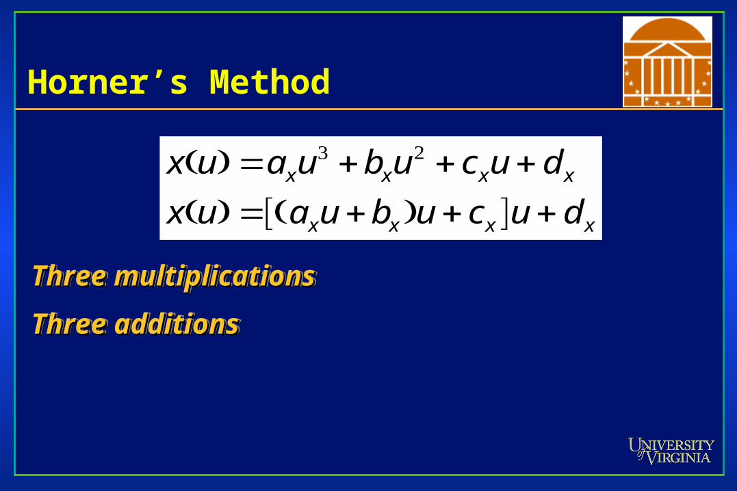
Horner’s Method
Three multiplicationsThree multiplications
Three additionsThree additions
Three multiplicationsThree multiplications
Three additionsThree additions
xxxx
xxxx
ducubuaux
ducubuaux
+++=+++=
])[()()( 23

Forward Difference
But this still is expensive to computeBut this still is expensive to compute
• Solve for change at k (Solve for change at k (kk) and change at k+1 () and change at k+1 (k+1k+1))
• Boot strap with initial values for xBoot strap with initial values for x00, , 00, and , and 11
• Compute xCompute x33 by adding x by adding x00 + + 00 + + 11
)()23(3
)()()(2322
1
231
23
1
δδδδδδ
δδδ
xxxkxxkxkkk
xkxkxkxk
xxxk
kkk
cbaubauaxxx
ducubuax
ducubuax
xxx
+++++==−
++++++=
+++=
+=
+
+
+

Subdivision Methods
BezierBezierBezierBezier

Rendering Bezier Spline
public void spline(ControlPoint p0, ControlPoint p1, ControlPoint p2, ControlPoint p3, int pix) { float len = ControlPoint.dist(p0,p1) + ControlPoint.dist(p1,p2) + ControlPoint.dist(p2,p3); float chord = ControlPoint.dist(p0,p3); if (Math.abs(len - chord) < 0.25f) return; fatPixel(pix, p0.x, p0.y); ControlPoint p11 = ControlPoint.midpoint(p0, p1); ControlPoint tmp = ControlPoint.midpoint(p1, p2); ControlPoint p12 = ControlPoint.midpoint(p11, tmp); ControlPoint p22 = ControlPoint.midpoint(p2, p3); ControlPoint p21 = ControlPoint.midpoint(p22, tmp); ControlPoint p20 = ControlPoint.midpoint(p12, p21); spline(p20, p12, p11, p0, pix); spline(p3, p22, p21, p20, pix); }