Crystallization of Synthetic Blast Furnace Slags …...Crystallization of Synthetic Blast Furnace...

Crystallization of Synthetic Blast Furnace Slags Pertaining to Heat Recovery

by

Shaghayegh Esfahani

A thesis submitted in conformity with the requirements for the degree of Doctor of Philosophy

Materials Science and Engineering University of Toronto

© Copyright by Shaghayegh Esfahani,

2016

ii

Crystallization of Blast Furnace Slags Pertaining to Heat

Recovery

Shaghayegh Esfahani

Doctorate

Materials Science and Engineering

University of Toronto

2016

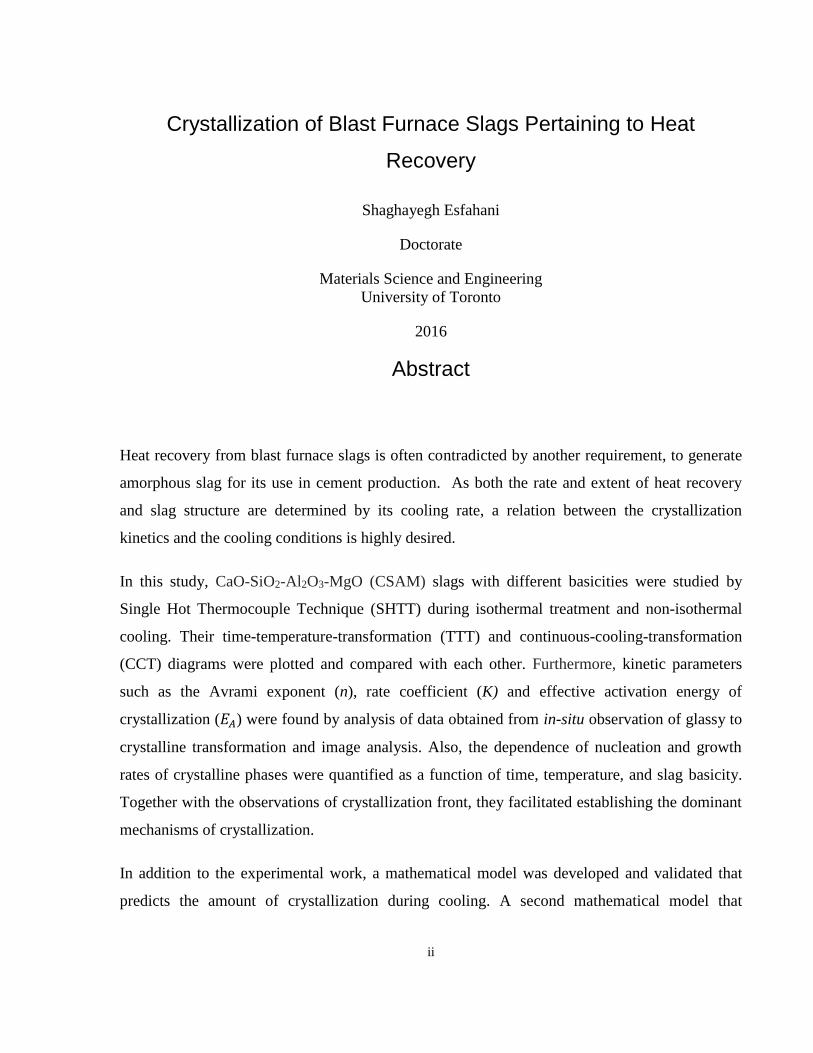
Abstract

Heat recovery from blast furnace slags is often contradicted by another requirement, to generate

amorphous slag for its use in cement production. As both the rate and extent of heat recovery

and slag structure are determined by its cooling rate, a relation between the crystallization

kinetics and the cooling conditions is highly desired.

In this study, CaO-SiO2-Al2O3-MgO (CSAM) slags with different basicities were studied by

Single Hot Thermocouple Technique (SHTT) during isothermal treatment and non-isothermal

cooling. Their time-temperature-transformation (TTT) and continuous-cooling-transformation

(CCT) diagrams were plotted and compared with each other. Furthermore, kinetic parameters

such as the Avrami exponent (n), rate coefficient (K) and effective activation energy of

crystallization (𝐸𝐴) were found by analysis of data obtained from in-situ observation of glassy to

crystalline transformation and image analysis. Also, the dependence of nucleation and growth

rates of crystalline phases were quantified as a function of time, temperature, and slag basicity.

Together with the observations of crystallization front, they facilitated establishing the dominant

mechanisms of crystallization.

In addition to the experimental work, a mathematical model was developed and validated that

predicts the amount of crystallization during cooling. A second mathematical model that

iii

calculates temperature history of slag during its cooling was coupled with the above model, to

allow studying the effect of parameters such as the slag/air ratio and granule size on the heat

recovery and glass content of slag.

iv

In the Name of God

To my parents, my husband and my brother…

v

Acknowledgments

First and foremost I offer my sincerest gratitude to my advisor and mentor, Prof. Mansoor Barati,

for his full support, patience and immense knowledge. I have been remarkably fortunate to have

a supervisor who gave me the freedom to explore on my own and at the same time provide full

guidance at any time that was needed.

I am grateful to all the members of my Ph.D. advisory committee, Prof. McLean, Prof. Stavros

Argyropolous, Prof. Ravi Ravindran and Prof. Charles Jia for their constructive suggestions.

I would also like to acknowledge my colleague Dr. Karim Danaei, Daniel Budurea from Dtek

Electronics Ltd. and Dr. Sina Mostaghel from Hatch Ltd. for their assistance.

I owe my deepest gratitude to my father and mother whose unwavering support and

unconditional love from thousands of miles away made this undertaking possible.

This thesis would not have been possible without my unbelievably supportive, patient and loving

husband, Dr. Farshid Bahrami. His continuous encouragement and endless love brightened the

most frustrating moments of my work and helped me move on. I would also like to thank my

brother, Matin, for being an extra source of inspiration and strength in my life, particularly

during the early years of being away from home.

I would like to thank the University of Toronto Open Fellowship, Ontario Government, Natural

Sciences and Engineering Research Council of Canada (NSERC) and Hatch Ltd. for their

financial support.

vi

Table of Contents

Acknowledgments............................................................................................................................v

Table of Contents ........................................................................................................................... vi

List of Figures ..................................................................................................................................x

List of Tables .............................................................................................................................. xvii

List of Symbols ............................................................................................................................ xix

List of Acronyms ......................................................................................................................... xxi

Chapter 1 ..........................................................................................................................................1

Introduction .................................................................................................................................1

Chapter 2 ..........................................................................................................................................5

Literature Review ........................................................................................................................5

Energy recovery from metallurgical slags ...........................................................................5

Metallurgical slags ...................................................................................................5

Use of slag as cement feedstock ..............................................................................7

Slag Granulation ......................................................................................................8

Energy content of slags ............................................................................................9

Review of energy recovery methods ......................................................................11

Evaluation of energy recovery methods ................................................................27

Crystallization of slag ........................................................................................................31

Summary ............................................................................................................................33

Chapter 3 ........................................................................................................................................36

Experimental .............................................................................................................................36

Hot Thermocouple Technique (HTT) ................................................................................36

vii

The Development of the hot thermocouple technique ...........................................37

Description of the hot thermocouple technique (HTT) ..........................................39

Modified HTT ........................................................................................................40

Hardware Controller ..............................................................................................43

Power supplies and thermocouple power driver ....................................................46

Verification of temperature measurement .............................................................47

Sample Preparation ............................................................................................................49

Experimental Procedure .....................................................................................................51

Isothermal Experiments .........................................................................................51

Continuous cooling experiment .............................................................................52

Chapter 4 ........................................................................................................................................54

Crystallization behavior ............................................................................................................54

Visualization of Crystallization .........................................................................................54

Slags with high basicity (NBO/T ≥ 1.71) ..............................................................54

Slags with low basicity (NBO/T<1.71) .................................................................58

Determination of the crystalline phases .............................................................................60

Time-Temperature-Transformation (TTT) diagram ..........................................................61

Continuous Cooling Transformation (CCT) diagram ........................................................63

Chapter 5 ........................................................................................................................................65

Prediction of the critical cooling rate ........................................................................................65

Critical Cooling Rate .........................................................................................................66

Relationship between slag composition and critical cooling rate ..........................68

Dependence of critical cooling rate on viscosity ...................................................69

Prediction of the critical cooling rate .................................................................................73

viii

Chapter 6 ........................................................................................................................................80

Kinetics of crystallization .........................................................................................................80

Theoretical treatment of transformation ............................................................................80

Experimental determination of phase change ....................................................................84

Determination of the Avrami exponent (n) and rate coefficient (k): .................................86

Nucleation ..........................................................................................................................89

Dependence of nucleation rate on temperature ......................................................89

Time dependency of nucleation rate ......................................................................91

Growth ...............................................................................................................................92

Activation energy of growth ..................................................................................97

Mechanism of slag crystallization .....................................................................................99

Effect of impingement on growth rate .............................................................................100

Effective activation energy of crystallization ..................................................................101

Chapter 7 ......................................................................................................................................110

Mathematical modeling of slag crystallization and heat recovery ..........................................110

Modeling the heat recovery process ................................................................................110

Assumptions .........................................................................................................110

Enthalpy method ..................................................................................................112

Enthalpy method vs. variable time step (VTS) method .......................................113

Numerical solution ...............................................................................................114

Analytical alternative of the “heat recovery” mathematical model .....................120

Temperature profile of slag droplets ....................................................................122

Modeling the amount of glassy content ...........................................................................123

Effect of operating parameters on heat recovery and slag structure ................................128

ix

Effect of air to slag ratio ......................................................................................128

Chapter 8 ......................................................................................................................................133

Contributions and conclusions ................................................................................................133

Conclusions ......................................................................................................................133

Contributions....................................................................................................................135

Publications ......................................................................................................................136

Future Research Directions .....................................................................................................138

Bibliography ................................................................................................................................140

Appendix A ..................................................................................................................................152

Appendix B ..................................................................................................................................153

x

List of Figures

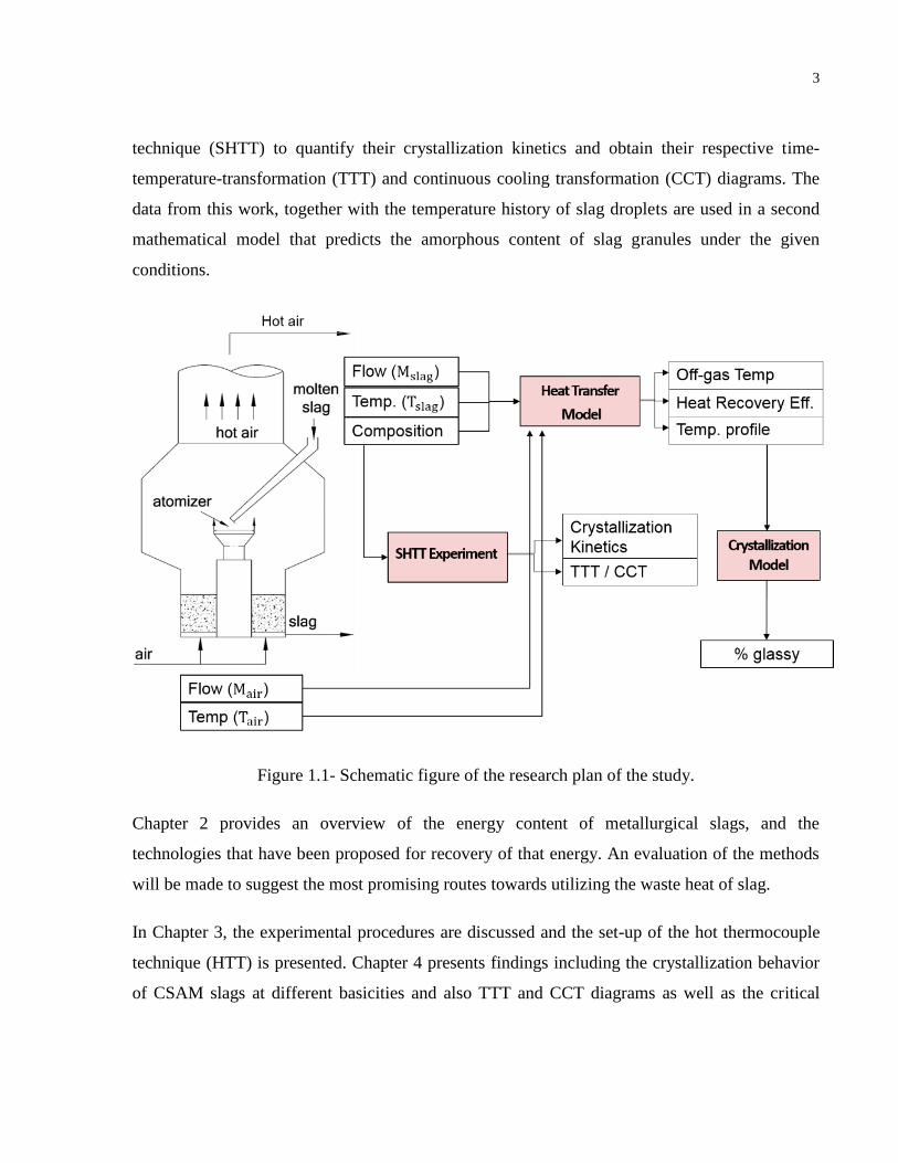
Figure 1.1- Schematic figure of the research plan of the study. ..................................................... 3

Figure 2.1- Temperature dependence of heat content for a typical blast-furnace slag [31]. ........ 11

Figure 2.2 - Temperature history of a 5 mm slag drop in fluidized bed [8]. ................................ 12

Figure 2.3 - Appearance of slag granulation by RCA with cup rotation speed of 3000 rpm [41].14

Figure 2.4 - Schematic diagram of Rotary Cup Atomizer [31]. ................................................... 14

Figure 2.5 - (a) slag atomization on the spinning disc and (b) granulated slag product [23, 50]. 16

Figure 2.6 - Process flow diagram of the rotary–drum granulation–heat recovery system [8]. ... 17

Figure 2.7 - Plant lay–out of Merotec slag granulation process [55]. ........................................... 18

Figure 2.8 - Schematic diagram of slag air granulation and heat recovery [26]. .......................... 19

Figure 2.9- Schematic of process developed by Paul Wurth [60]. ............................................... 20

Figure 2.10- Schematic of the process developed by JFE [62]. .................................................... 21

Figure 2.11 - Process flow diagram for energy recovery through methane reforming [42]. ........ 23

Figure 2.12 - Steam reforming of methane using granulated slag heat [64]. ................................ 24

Figure 2.13 – Coal gasification process [67]. ............................................................................... 26

Figure 2.14 - Steam reforming of methane using granulated slag heat [64]. ................................ 30

Figure 2.15- TTT diagram of BF slag by Kashiwaya et al. [72]. ................................................. 31

Figure 2.16 – CCT diagram of BF slag by Kashiwaya et al. [72]. .............................................. 31

xi

Figure 2.17- TTT diagram of BF slag by Qin et al. [73]. ............................................................. 32

Figure 2.18- CCT diagram of BF slag by Qin et al. [73]. ............................................................ 32

Figure 2.19 – TTT diagram of synthetic BF slag with varying Al2O3 content by Sun et al. [66].

CaO/SiO2=1.0, A1=11wt%, A2=20wt%, A3=23wt% .................................................................. 33

Figure 3.1 - Basic circuit diagram of the first hot thermocouple apparatus (a) by Ordway [96] (b)

by Welch [97]. .............................................................................................................................. 38

Figure 3.2 - Comparison of the single and double hot thermocouple setups [77]. ....................... 39

Figure 3.3 - Schematic of the thermocouple tip. ........................................................................... 40

Figure 3.4 - Schematic view of the HTT setup. ............................................................................ 40

Figure 3.5 – Schematic figure showing the principal of AC based HT controller [77]. ............... 41

Figure 3.6 – Schematic figure showing the principal of the modified DC based HT controller. . 41

Figure 3.7 - Simplified block diagram of the new concept target design. .................................... 43

Figure 3.8 - Hot thermocouple controller block diagram. ............................................................ 45

Figure 3.9 - Schematic diagram of the timing of the power supply and acquisition. ................... 46

Figure 3.10 - Melting temperature measurement for HTT apparatus calibration a) Na2SO4 b)

CaF2............................................................................................................................................... 48

Figure 3.11 - Derivative of the time-temperature curve for Na2SO4. ........................................... 48

Figure 3.12 - XRD analysis of slag with C/S=1.18 after water quenching. ................................. 50

Figure 3.13 - Pseudo-ternary diagram of the slag system; MgO-CaO-SiO2 with 15 wt % Al2O3

[103]. ............................................................................................................................................. 51

xii

Figure 3.14 - Heat treatment of slag samples: a) isothermal heat treatment b) schematic TTT

diagram plotted from isothermal heat treatment experiments c) continuous cooling ................... 52

Figure 3.15 - Crystallization of slag with C/S=1.31 during continuous cooling (cooling rate=

~1°C.s-1). ....................................................................................................................................... 52

Figure 4.1 - Equiaxed growth at 1380°C isotherm (NBO/T=1.94). ............................................. 55

Figure 4.2- Enlarged images showing (a) equiaxed crystals of sample with NBO/T=1.71 at

1300°C (b) elongated crystals of sample with NBO/T=1.94 at 1150°C. ...................................... 55

Figure 4.3 - Mixed planar and equiaxed growth at 1320ºC isotherm (NBO/T=1.94). ................. 56

Figure 4.4 - Planar growth at 1300°C isotherm (NBO/T=1.94). .................................................. 56

Figure 4.5 - Faceted and planar growth at 1170°C isotherm (NBO/T=1.71). .............................. 57

Figure 4.6 – Elongated crystallization at 1150°C isotherm (NBO/T=1.94). ................................ 58

Figure 4.7 - Crystallization of slag with NBO/T=1.94 at 1100°C isotherm. ................................ 58

Figure 4.8- Crystallization of slag NBO/T=1.56 at 1250°C isotherm. ......................................... 59

Figure 4.9 - Crystallization of slag NBO/T=1.56 at 1150°C isotherm. ........................................ 59

Figure 4.10 - TTT Diagram for samples with (a) NBO/T= 1.18 (b) NBO/T = 1.44 (c) NBO/T

=1.56 (d) NBO/T=1.71(e) NBO/T = 1.78 (f) NBO/T =1.94. ....................................................... 62

Figure 4.11 - Start curves of the TTT diagrams. ........................................................................... 63

Figure 4.12 - CCT Diagram for slag samples with (a) NBO/T = 1.44 (b) NBO/T = 1.56 (c)

NBO/T = 1.71(d) NBO/T = 1.78 (e) NBO/T = 1.94 (f) Comparison of all CCT diagrams. ........ 64

Figure 5.1 - RC from TTT diagram vs. NBO/T and Λ𝑐𝑜𝑟𝑟. .......................................................... 67

Figure 5.2 - Relationship between slag composition and critical cooling rate. ............................ 69

xiii

Figure 5.3 - RC and 𝜂𝑛𝑜𝑠𝑒 Pa. s vs. Λ𝑐𝑜𝑟𝑟. ................................................................................... 70

Figure 5.4 - Correlation between slag composition and viscosity at liquidus temperature (𝜂𝑙). .. 71

Figure 5.5 - Log 𝑅𝑐 vs. Log (𝜂𝑛𝑜𝑠𝑒/ Pa.s). .................................................................................. 72

Figure 5.6 - 𝐿𝑜𝑔 𝜂𝑛𝑜𝑠𝑒 and 𝑙𝑜𝑔 𝜂L vs. 𝐿𝑜𝑔 𝑅𝐶........................................................................... 73

Figure 5.7 – Critical cooling rate against 𝜆 ................................................................................... 76

Figure 5.8 - from TTT vs. predicted. ............................................................................... 79

Figure 6.1 - An illustration of the concept of extended volume (𝑉𝑒). (a) Two precipitate crystals

have nucleated together and grown to a finite size in the time t. (b) New regions (shown as

lighter grey) are formed as the original crystals grow. These regions are no longer available for

newer crystals to nucleate from [117]. .......................................................................................... 81

Figure 6.2 - Crystallization of slag with C/S=1.52 at 1200°C isotherm (𝜏 =incubation time). .... 85




Figure 6.6 - (a) Crystallized fraction as a function of time (b) JMAK plots for the slag with

C/S=1.52. ...................................................................................................................................... 87


C/S=1.38. ...................................................................................................................................... 87


C/S=1.31 ....................................................................................................................................... 88


C/S=1.18 ....................................................................................................................................... 88

CR CR

xiv

Figure 6.10 – Dependence of nucleation rate on the temperature range of 𝑇 − 𝑇𝐿 [134]. .......... 90

Figure 6.11 - 𝐿𝑛 𝑁 rate verses 1/𝑇 for all samples in the early stage of nucleation. ................... 91

Figure 6.12 - Nucleation in slag with C/S=1.38 at T= 1170°C after (a) 10s (b) 11s. ................... 92

Figure 6.13 - Change of nucleation rate with time for all slags at T=1200°C . ............................ 92

Figure 6.14 - Growth rate measurement for sample with C/S=1.38 at T=1250°C (a) 𝑡 − 𝜏=3s .. 93

Figure 6.15 - Crystal thickness verses time (a) C/S=1.52 (b) C/S=1.38 (c) C/S=1.31 (d)

C/S=1.18. ...................................................................................................................................... 94

Figure 6.16 - Dependence of growth rate on basicity. .................................................................. 95

Figure 6.17 - Interface morphology for sample with C/S=1.18 at (a) T=1250°C the interface is

fully dendritic (b) T=1200°C semi-dendritic (c) T=1130°C planar. ............................................. 96

Figure 6.18 - 𝐺 verses (1/𝑇). ...................................................................................................... 98

Figure 6.19 - Change of activation energy of growth with basicity. ............................................ 99

Figure 6.20 - Effect of impinging on the growth rate for sample with C/S=1.18 at T=1150°C after

(a) 10s (b) 70s (c) 80s. ................................................................................................................ 101

Figure 6.21 - Growth rate change with collision of neighboring crystals. ................................. 101

Figure 6.22 - 𝐿𝑛𝐾 vs. 1/𝑅𝑇 (C/S=1.52). .................................................................................... 103



Figure 6.25 - TTT diagram of the slags. ..................................................................................... 105


xv

Figure 6.27 - XRD spectrums of slag with C/S=1.38 at T=1150°C and T=1250 °C. ................. 106

Figure 6.28 - XRD spectrums of slag with C/S=1.18 at T=1150°C and T=1250°C. .................. 107

Figure 6.29 - 𝐿𝑛𝐾 verses 1/𝑅𝑇 for all slag compositions. ........................................................ 108

Figure 7.1 - Schematic diagram of the model principal.............................................................. 111

Figure 7.2 - Schematic figure of enthalpy-temperature function for (a) pure crystalline material

..................................................................................................................................................... 113

Figure 7.3 - H-T relationship for slag with 47% CaO, 33%, SiO2, 15% Al2O3, 5%MgO. ......... 118

Figure 7.4 - Effect of the number of layers (𝑀) on the contact time. ......................................... 119

Figure 7.5 - Comparison between the experimental results of [150] and the model outputs for

position of the solidification front in a lead droplet. r/R= is the position of the liquid-solid

interface from center of lead sphere (cm). .................................................................................. 120

Figure 7.6 - Analytical solution compared with modeling result (constant air temperature without

phase change). ............................................................................................................................. 121

Figure 7.7 - Comparing temperature profiles from analytical solution and numerical modeling

(constant air temperature with phase change). ............................................................................ 122

Figure 7.8 - Temperature profile of slag droplets at 𝑀𝑎𝑖𝑟𝑀𝑠𝑙𝑎𝑔 = 0.77 and D=5mm. ........... 123

Figure 7.9 - (a) approximation of a continuous cooling curve with a series of isothermals and (b)

adding transformed contents at different temperature validation of model. ............................... 125

Figure 7.10 - Validation of the model for predicting phase transformation by using TTT diagram

and cooling path. The green points show the results by Agarwal et al. [152] and the smaller blue

dots show the results by the existing code. ................................................................................. 126

Figure 7.11 - TTT diagram (C/S=1.31). ..................................................................................... 127

xvi

Figure 7.12 - Crystallized fraction during continuous transformation (2°C/s) from experimental

measurement and predicted by the code (C/S=1.31). ................................................................. 127

Figure 7.13 - CCT obtained from experimental measurements and modeling calculations

(C/S=1.31). .................................................................................................................................. 128

Figure 7.14 - Heat recovery efficiency, air exit temperature, and amorphous content of slag as a

function of 𝑀𝑎𝑖𝑟/𝑀𝑠𝑙𝑎𝑔for slag with C/S=1.52 and D=8mm. .................................................. 130

Figure 7.15 - Effect of droplet size on the heat recovery efficiency. .......................................... 131

Figure 7.16 - Effect of droplet size on contact time. .................................................................. 131

Figure 7.17 - Effect of droplet size on air exit temperature. ....................................................... 132

Figure 9.1 - End time of crystallization for sample with C/S=1 with and without Cr2O3 at T=1100

°C isotherm (repeated 14 times). ................................................................................................ 138

xvii

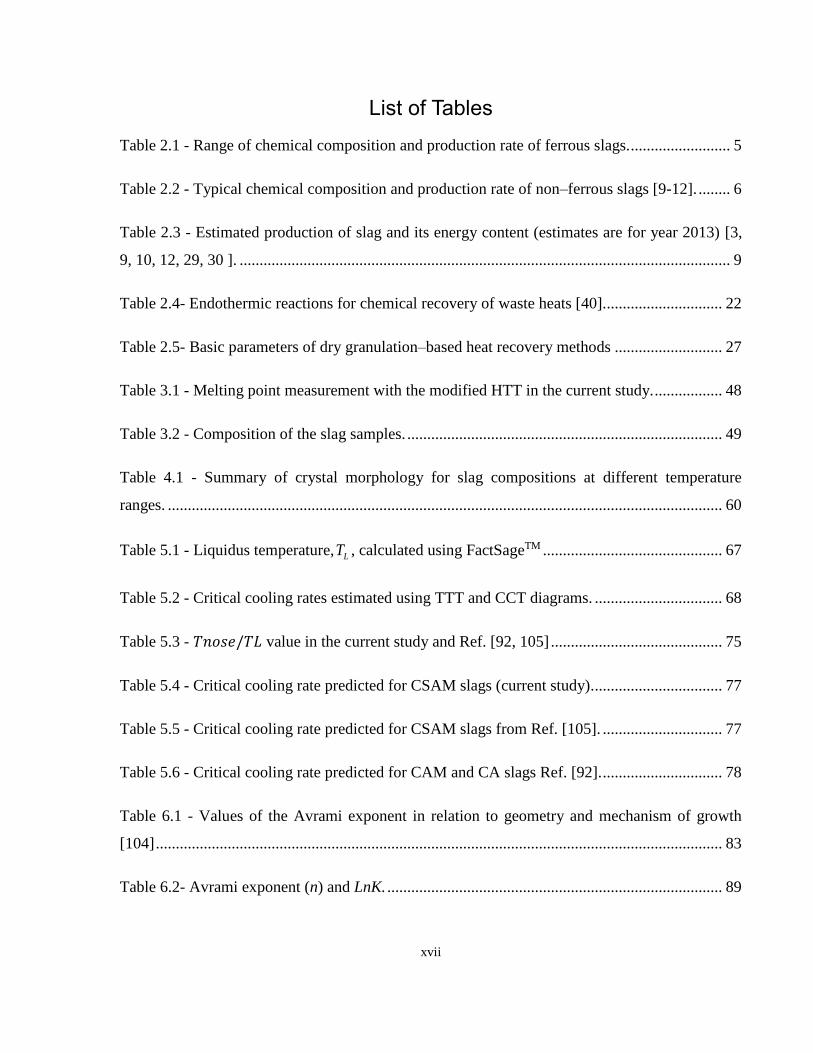
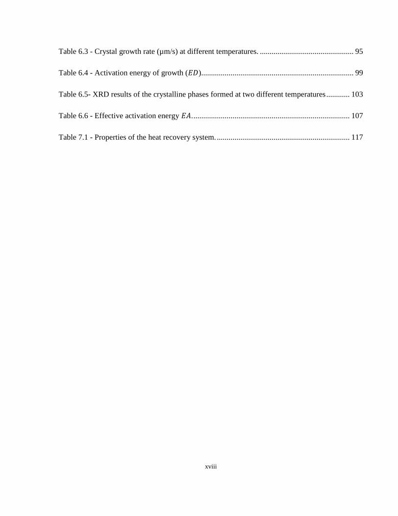
List of Tables

Table 2.1 - Range of chemical composition and production rate of ferrous slags. ......................... 5

Table 2.2 - Typical chemical composition and production rate of non–ferrous slags [9-12]. ........ 6

Table 2.3 - Estimated production of slag and its energy content (estimates are for year 2013) [3,

9, 10, 12, 29, 30 ]. ........................................................................................................................... 9

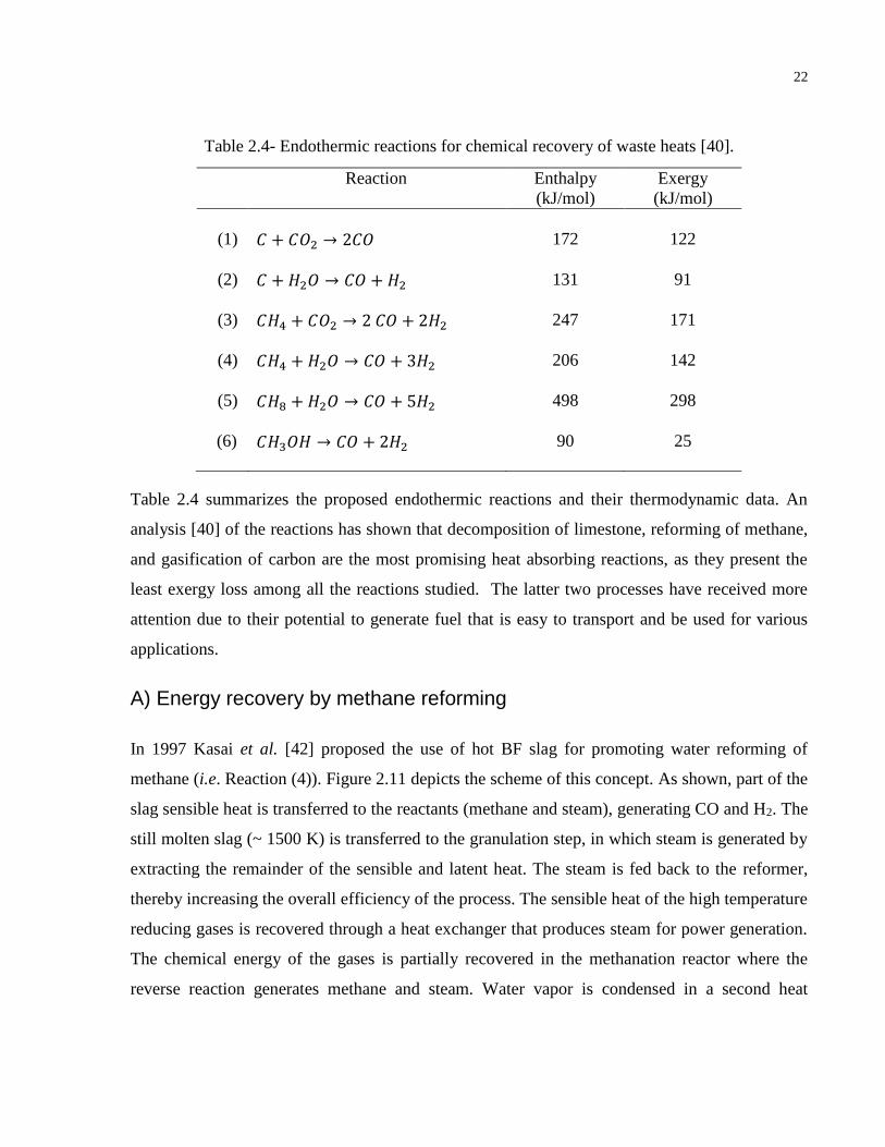
Table 2.4- Endothermic reactions for chemical recovery of waste heats [40]. ............................. 22

Table 2.5- Basic parameters of dry granulation–based heat recovery methods ........................... 27

Table 3.1 - Melting point measurement with the modified HTT in the current study. ................. 48

Table 3.2 - Composition of the slag samples. ............................................................................... 49

Table 4.1 - Summary of crystal morphology for slag compositions at different temperature

ranges. ........................................................................................................................................... 60

Table 5.1 - Liquidus temperature, , calculated using FactSageTM ............................................. 67

Table 5.2 - Critical cooling rates estimated using TTT and CCT diagrams. ................................ 68

Table 5.3 - 𝑇𝑛𝑜𝑠𝑒/𝑇𝐿 value in the current study and Ref. [92, 105] ........................................... 75

Table 5.4 - Critical cooling rate predicted for CSAM slags (current study)................................. 77

Table 5.5 - Critical cooling rate predicted for CSAM slags from Ref. [105]. .............................. 77

Table 5.6 - Critical cooling rate predicted for CAM and CA slags Ref. [92]. .............................. 78

Table 6.1 - Values of the Avrami exponent in relation to geometry and mechanism of growth

[104] .............................................................................................................................................. 83

Table 6.2- Avrami exponent (n) and LnK. .................................................................................... 89

LT

xviii

Table 6.3 - Crystal growth rate (µm/s) at different temperatures. ................................................ 95

Table 6.4 - Activation energy of growth (𝐸𝐷). ............................................................................. 99

Table 6.5- XRD results of the crystalline phases formed at two different temperatures ............ 103

Table 6.6 - Effective activation energy 𝐸𝐴. ................................................................................ 107

Table 7.1 - Properties of the heat recovery system. .................................................................... 117

xix

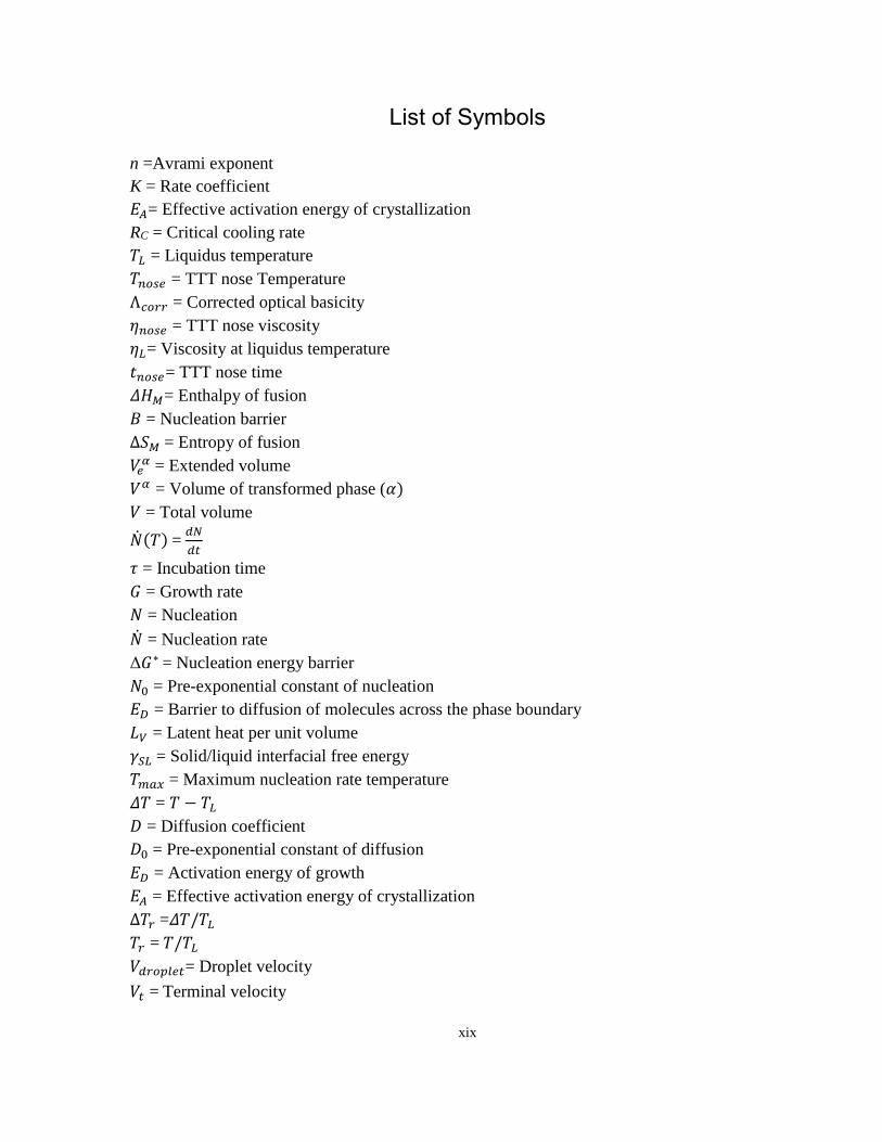
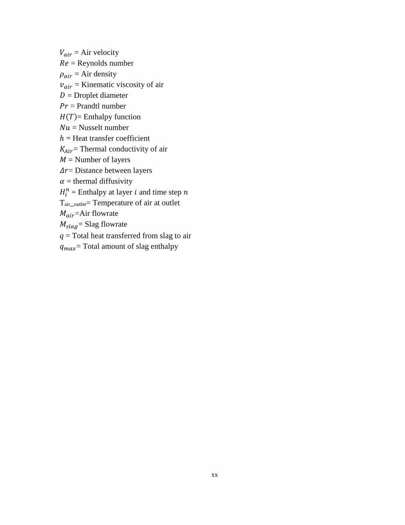
List of Symbols

n =Avrami exponent

K = Rate coefficient

𝐸𝐴= Effective activation energy of crystallization

RC = Critical cooling rate

𝑇𝐿 = Liquidus temperature

𝑇𝑛𝑜𝑠𝑒 = TTT nose Temperature

Λ𝑐𝑜𝑟𝑟 = Corrected optical basicity

𝜂𝑛𝑜𝑠𝑒 = TTT nose viscosity

𝜂𝐿= Viscosity at liquidus temperature

𝑡𝑛𝑜𝑠𝑒= TTT nose time

𝛥𝐻𝑀= Enthalpy of fusion

𝐵 = Nucleation barrier

∆𝑆𝑀 = Entropy of fusion

𝑉𝑒𝛼 = Extended volume

𝑉𝛼 = Volume of transformed phase (𝛼)

𝑉 = Total volume

��(𝑇) = 𝑑𝑁

𝑑𝑡

𝜏 = Incubation time

𝐺 = Growth rate

𝑁 = Nucleation

�� = Nucleation rate

Δ𝐺∗ = Nucleation energy barrier

𝑁0 = Pre-exponential constant of nucleation

𝐸𝐷 = Barrier to diffusion of molecules across the phase boundary

𝐿𝑉 = Latent heat per unit volume

𝛾𝑆𝐿 = Solid/liquid interfacial free energy

𝑇𝑚𝑎𝑥 = Maximum nucleation rate temperature

𝛥𝑇 = 𝑇 − 𝑇𝐿

𝐷 = Diffusion coefficient

𝐷0 = Pre-exponential constant of diffusion

𝐸𝐷 = Activation energy of growth

𝐸𝐴 = Effective activation energy of crystallization

Δ𝑇𝑟 =𝛥𝑇/𝑇𝐿

𝑇𝑟 = 𝑇/𝑇𝐿

𝑉𝑑𝑟𝑜𝑝𝑙𝑒𝑡= Droplet velocity

𝑉𝑡 = Terminal velocity

xx

𝑉𝑎𝑖𝑟 = Air velocity

𝑅𝑒 = Reynolds number

𝜌𝑎𝑖𝑟 = Air density

𝑣𝑎𝑖𝑟 = Kinematic viscosity of air

𝐷 = Droplet diameter

𝑃𝑟 = Prandtl number

𝐻(𝑇)= Enthalpy function

𝑁𝑢 = Nusselt number

ℎ = Heat transfer coefficient

𝐾𝐴𝑖𝑟= Thermal conductivity of air

𝑀 = Number of layers

𝛥𝑟= Distance between layers

𝛼 = thermal diffusivity

𝐻𝑖𝑛 = Enthalpy at layer 𝑖 and time step 𝑛

Tair_outlet= Temperature of air at outlet

𝑀𝑎𝑖𝑟=Air flowrate

𝑀𝑠𝑙𝑎𝑔= Slag flowrate

q = Total heat transferred from slag to air

𝑞𝑚𝑎𝑥= Total amount of slag enthalpy

xxi

List of Acronyms

TTT = Time temperature transformation

CCT = Continuous cooling transformation

HTT = Hot thermocouple technique

CSAM = CaO-SiO2-Al2O3-MgO

C/S = CaO/SiO2

GBFS = Granulated blast furnace slag

RCA = Rotary cup atomizer

ACQ = Acquisition

AC = Alternated current

DC = Direct current

MCU = Microcontroller unit

PC = Personal computer

SW = Software

A/D = Analog to Digital

ADC = Analog to Digital Converter

IC = Integrated circuit

TC = Thermocouple

PWM = Pulse Width Modulation

IA = Instrumentation Amplifier

TRIAC = Triode for Alternating Current

MOSFET = Metal-Oxide Semiconductor Field Effect Transistor

SCR = Silicon controlled rectifier

NBO/T = non-bridging oxygen atoms over tetrahedrally coordinated atoms

JMAK = Johnson-Mehl-Avrami-Kolmogorov

HRE = Heat recovery efficiency

1

Chapter 1

Introduction

Metal manufacturing industry has achieved tremendous improvements in its energy efficiency in

the past several decades. The specific energy consumption of steel in the U.S., for instance, has

decreased from 48 to 20 MJ/ton in the period 1960–2000 [1]. This accomplishment has been

realized by implementing numerous technological advancements such as introduction of

continuous and chained operations where the regular cooling–heating cycles between the

processing steps are eliminated. In a study, Fruehan et al. [2] estimated the potential energy

saving in steel manufacturing and showed that there is an opportunity to further reduce the

energy consumption involved in making liquid steel by about 20–30%. With established

technologies to recover the thermal and chemical energies of process off–gas, the waste heat of

slags presents the last untapped source that may be used for energy conservation in the rather

energy–intensive metals industry.

Metallurgical slags constitute the largest by–product of the high temperature operations involved

in the extraction and refining of metals. Slags are comparable to molten lava and are generally

rich in silica (SiO2), alumina (Al2O3), and lime (CaO). Slag is formed from the refining

reactions, remaining gangue of the ore, the erosion of the furnace refractory, and the added

fluxes. The molten slag is tapped at temperatures up to 1650°C, carrying a substantial amount of

high quality thermal energy. This energy is usually not recovered, as the slag is tapped and

cooled in the ambient or rapidly quenched to make glassy granules that are used as feedstock for

cement manufacturing. Over the past four decades, several processes have been proposed to

recover the waste energy of slag as heat, electricity, and fuel, while none has been

commercialized yet. A renewed attempt at evaluation of the proposed processes is critical, as the

metals industry is striving for another major step in improving its energy efficiency.

2

Blast furnace slags constitute over 50% of the total slag produced worldwide, amounting to 320

million tonnes. The thermal energy of these slags is equal to 17 million tonnes of coal, and is

currently not recovered [3], in large due to challenge of heat recovery while producing a valuable

product from slag. Blast furnace slags are most desired as feedstock for Portland cement

production due to the large contents of silica and lime in these slags. For this application blast

furnace slag has to be cooled rapidly to form an amorphous structure, as otherwise it will cause

swelling of the concrete made from slag cement. Up to now, this is achieved by quenching slag

in a process known as wet granulation. However, the use of water does not allow recovery of

slag. In order to overcome this problem, dry granulation and heat recovery using air has been

suggested. The optimum conditions for such air-based cooling system are not known yet; one on

hand, large amounts of air are required to ensure rapid cooling, while on the other hand smaller

amount of air is preferred to recovery the thermal energy into air as high grade heat. Therefore,

one of the most important parameters to be determined is critical cooling rate which is a cooling

rate that is just enough to generate glassy slag without consuming too much air. Further, the

effect of slag composition on the critical cooling rate, and how such cooling conditions can be

applied to slag are required. The present study was undertaken with the aim of answering these

questions (a) understand the crystallization behavior of blast furnace type slags in order to

determine the critical cooling rate and its relation to composition, (b) investigate the possibility

of manipulating slag chemistry for achieving the desired structure, (c) determining the optimum

conditions of a heat recovery process in terms of slag/air ratio, granule size, heat recovery vessel

dimensions, and slag composition for highest heat grade, while generating a glassy product.

Different chapters of the thesis cover the research approach and the findings as discussed below,

and Figure 1.1 illustrates the summary of the research plan in the study. Essentially, we consider

a heat recovery duct in which granule slag drops are descending in a counter-current flow of air.

The flow rate, temperature, and composition of slag, as well as the flow rate and temperature of

air are used in a heat transfer model, to calculate cooling profile of slag granules from their

surface to core. In addition, the model predicts the exit temperature of air, as well as the heat

transfer efficiency, being measures of heat quality and heat recovery efficiency respectively. The

slags of various compositions are studied experimentally using a single hot thermocouple

3

technique (SHTT) to quantify their crystallization kinetics and obtain their respective time-

temperature-transformation (TTT) and continuous cooling transformation (CCT) diagrams. The

data from this work, together with the temperature history of slag droplets are used in a second

mathematical model that predicts the amorphous content of slag granules under the given

conditions.

Figure 1.1- Schematic figure of the research plan of the study.

Chapter 2 provides an overview of the energy content of metallurgical slags, and the

technologies that have been proposed for recovery of that energy. An evaluation of the methods

will be made to suggest the most promising routes towards utilizing the waste heat of slag.

In Chapter 3, the experimental procedures are discussed and the set-up of the hot thermocouple

technique (HTT) is presented. Chapter 4 presents findings including the crystallization behavior

of CSAM slags at different basicities and also TTT and CCT diagrams as well as the critical

4

cooling rate. Later, in Chapter 5 the prediction of the critical cooling rate is discussed. The

kinetic behavior of crystallization including nucleation and growth and Avrami parameters was

also studied and is presented in Chapter 6. Chapter 7 of this thesis provides the details of the two

mathematical models that were developed for slag crystallization and heat recovery. Finally in

the last chapter the conclusion of the study is provided.

5

Chapter 2

Literature Review

Energy recovery from metallurgical slags

Metallurgical slags

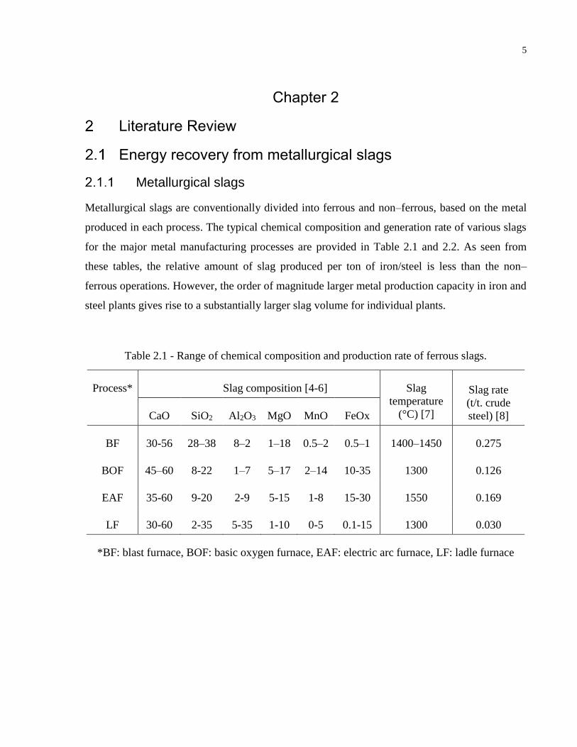
Metallurgical slags are conventionally divided into ferrous and non–ferrous, based on the metal

produced in each process. The typical chemical composition and generation rate of various slags

for the major metal manufacturing processes are provided in Table 2.1 and 2.2. As seen from

these tables, the relative amount of slag produced per ton of iron/steel is less than the non–

ferrous operations. However, the order of magnitude larger metal production capacity in iron and

steel plants gives rise to a substantially larger slag volume for individual plants.

Table 2.1 - Range of chemical composition and production rate of ferrous slags.

Process* Slag composition [4-6] Slag

temperature

(°C) [7]

Slag rate

(t/t. crude

steel) [8] CaO SiO2 Al2O3 MgO MnO FeOx

BF 30-56 28–38 8–2 1–18 0.5–2 0.5–1 1400–1450 0.275

BOF 45–60 8-22 1–7 5–17 2–14 10-35 1300 0.126

EAF 35-60 9-20 2-9 5-15 1-8 15-30 1550 0.169

LF 30-60 2-35 5-35 1-10 0-5 0.1-15 1300 0.030

*BF: blast furnace, BOF: basic oxygen furnace, EAF: electric arc furnace, LF: ladle furnace

6

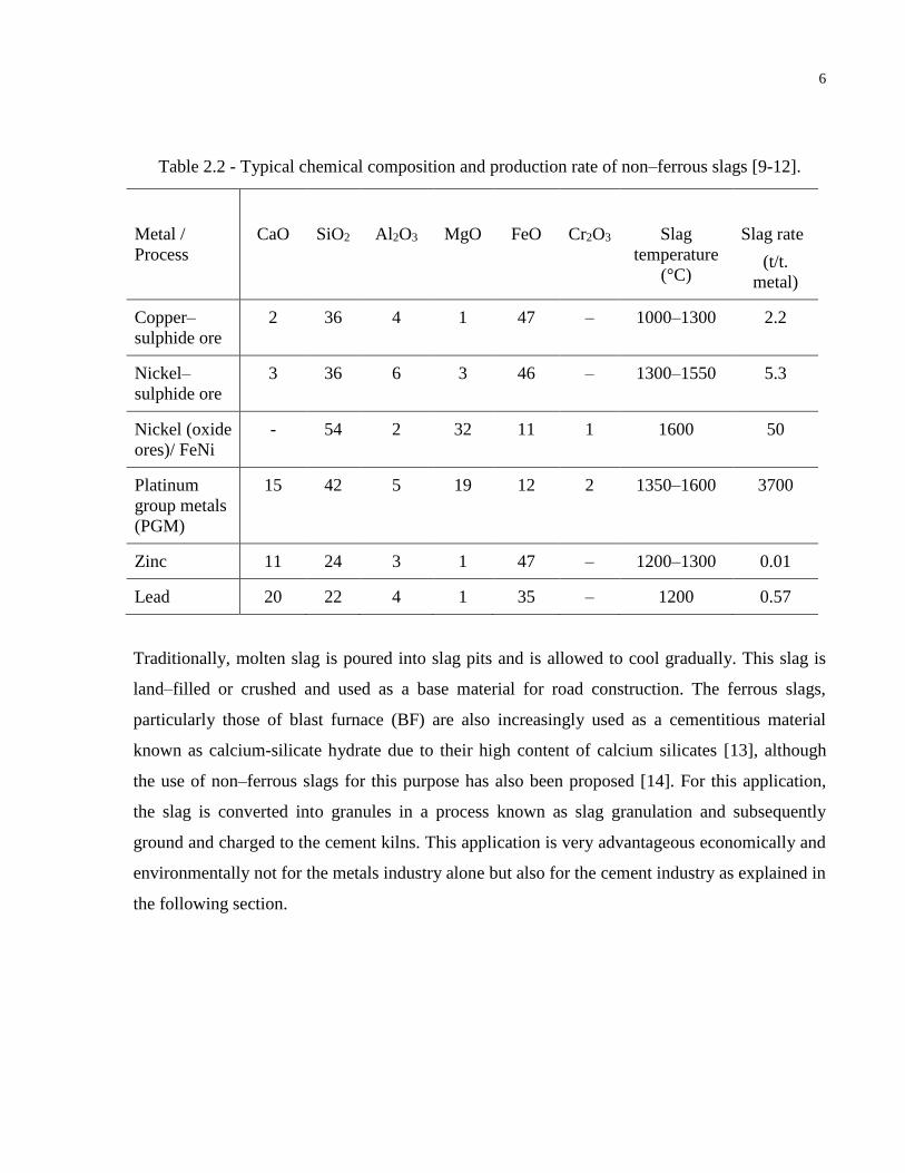
Table 2.2 - Typical chemical composition and production rate of non–ferrous slags [9-12].

Metal /

Process

CaO

SiO2

Al2O3

MgO

FeO

Cr2O3

Slag

temperature

(°C)

Slag rate

(t/t.

metal)

Copper–

sulphide ore

2 36 4 1 47 – 1000–1300 2.2

Nickel–

sulphide ore

3 36 6 3 46 – 1300–1550 5.3

Nickel (oxide

ores)/ FeNi

- 54 2 32 11 1 1600 50

Platinum

group metals

(PGM)

15 42 5 19 12 2 1350–1600 3700

Zinc 11 24 3 1 47 – 1200–1300 0.01

Lead 20 22 4 1 35 – 1200 0.57

Traditionally, molten slag is poured into slag pits and is allowed to cool gradually. This slag is

land–filled or crushed and used as a base material for road construction. The ferrous slags,

particularly those of blast furnace (BF) are also increasingly used as a cementitious material

known as calcium-silicate hydrate due to their high content of calcium silicates [13], although

the use of non–ferrous slags for this purpose has also been proposed [14]. For this application,

the slag is converted into granules in a process known as slag granulation and subsequently

ground and charged to the cement kilns. This application is very advantageous economically and

environmentally not for the metals industry alone but also for the cement industry as explained in

the following section.

7

Use of slag as cement feedstock

It has been shown that substituting earth minerals with slag could give rise to up to 50 percent

reduction in the CO2 emissions associated with production of Portland cement [15]. Other than

reducing CO2 emissions, using slag cement instead of Portland cement has many other benefits,

the most important of which is discussed in the following paragraphs.

Advantages of using slag cement

A) Environmental benefits

Cement production is an energy intensive partly due to the energy needed for calcination of

limestone. Using slag can lower the energy consumption of cement making significantly.

Producing an equal volume of slag will require 90% less energy than Portland cement. It has

been discussed that substituting 50% of cement feed with slag can reduce the energy

consumption up to 34% [16]. In addition, usage of slag cement reduces the “urban heat island”

effect by enabling concrete to reflect more light and cooling structures due to the lighter color of

slag cement compared with Portland cement [17].

B) Higher quality

Concrete containing slag powder has higher strength and durability as a result of less

permeability. In addition, because of the reduced unit volume, concrete will have higher

resistance against alkli-silica and sulfate attack which in return extends the life of concrete.

Furthermore, slag cement reduces the temperature difference between the surface and the center

of concrete in large structures which guards against thermal cracking.

C) Reduced material extraction

Raw materials for Portland cement require mining and processing. For every ton of Portland

cement, 1.6 tons of raw materials is extracted. Substitution of raw minerals by slag reduces the

need for extraction of raw materials significantly.

8

Demand for slag cement

Currently over 200 Mt/year of granulated blast furnace slag (GBFS) cement is used worldwide

which is approximately equal to 62% of the total amount of blast furnace slag that was produced

in the year 2013 [18]. Considering 50-80% of this type of cement contains BF slag [19], it is

estimated that each year 100-160 Mt of slag is sold to the cement industry. According to the

USGS survey, each ton of GBFS was sold for as high as $100 in the year 2011 [20]. Based on

these figures, the value of the total amount of BF slag sold to the cement industry would be

approximately $10-16 billion. Furthermore, if the total heat of this slag was recovered it would

be about 45-70 TWh/y adding a value of $4.5-7 billion. This demonstrates the significance of

heat recovery from slags during granulation process which will further be discussed in the

following sections.

Slag Granulation

The slag used as a cement feedstock needs to be in amorphous form (i.e. glassy) to avoid

subsequent swelling of the concrete. Consequently, the granulation processes use pressurized

water, wet granulation, or large quantities of air, dry granulation, to prevent slow cooling and

crystallization of the slag during solidification. Cooling rates in excess of 10°C/s [21] are

required to form an amorphous slag with sufficiently strong hydaulicity.

Despite the effectiveness of wet granulation in producing a glassy slag, the thermal energy

contained in the high temperature slag is not recovered. In addition, the wet process uses a large

amount of water for granulation, typically around 10 tonnes of water of which 1–1.5 tonnes

evaporates per tonne of slag [22-24]. Leaching of alkaline oxides in water and release of H2S gas

are other environmental problems associated with wet granulation. Dry granulation, on the other

hand presents an opportunity to simultaneously generate a glassy slag and recover the sensible

heat in the form of hot gases, steam, or chemical energy. As a result, the attempts to recover slag

waste heat have been focused on dry granulation.

The attempts for dry granulation of slag date back to 1930 [25], but the research surged in 1970s

and 1980s in Europe and Japan, resulting in laboratory and pilot scale testing of several methods.

9

In Section 2.1.5, the processes that have been proposed for energy recovery from slag, based on

the use of dry granulation are described.

Energy content of slags

The energy consumed in high temperature processing of metals is distributed between metal,

slag, off–gas, and the natural losses to the refractories and atmosphere. The slag thermal energy

represents about 10–90% of the output energy depending on the slag/metal ratio and the

discharge temperature. For instance, Rodd et al. [26] concluded that for ferro–nickel production,

slag represents approximately 80% of the total energy input into the electric smelting furnaces.

For steel production, on the other hand, estimated share of slag energy is 10–15% [27, 28].

Nevertheless, on a world basis the total amount of energy contained ins slag is substantial for all

metals (Table 2.3).

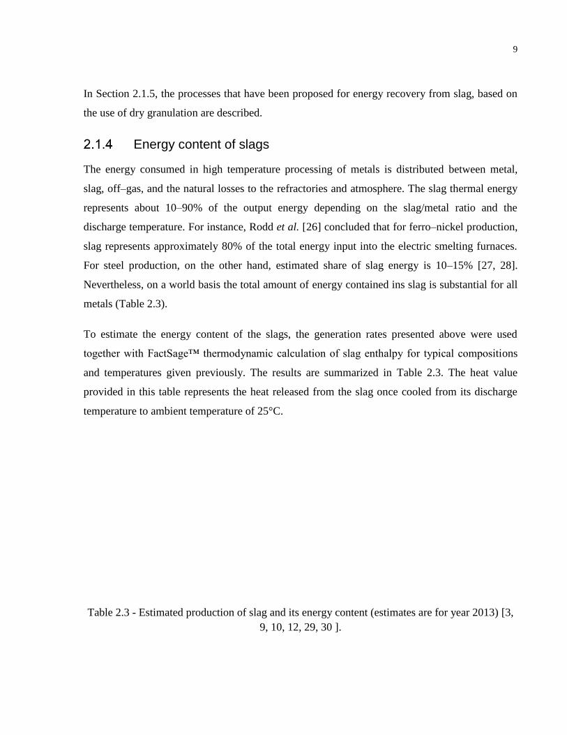
To estimate the energy content of the slags, the generation rates presented above were used

together with FactSage™ thermodynamic calculation of slag enthalpy for typical compositions

and temperatures given previously. The results are summarized in Table 2.3. The heat value

provided in this table represents the heat released from the slag once cooled from its discharge

temperature to ambient temperature of 25°C.

Table 2.3 - Estimated production of slag and its energy content (estimates are for year 2013) [3,

9, 10, 12, 29, 30 ].

10

Slag Temp. Slag

Enthalpy Slag Production Energy Value

Process/

Metal

°C GJ/tonne Million Tonnes GJ TWh

Million t

Coal

Equiv.

Blast furnace 1400-1450 1.6 321.3 5.14×108 142.8 17.1

Other ferrous

processes 1300-1600 1.3-1.8 292.0 4.37×108 121.5 14.6

Non-ferrous

Metals 1000-1600 1.2-1.5 52.0 6.55×108 18.2 2.2

Total 665.2 1.02×109 282.5 33.9

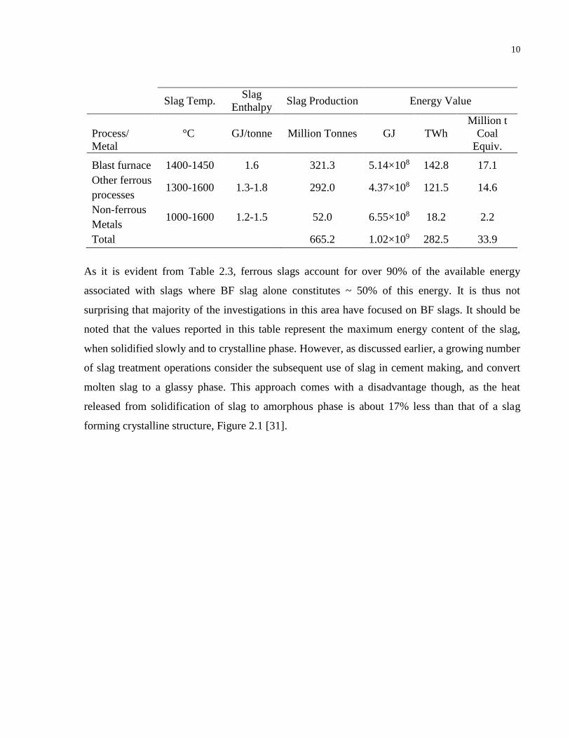
As it is evident from Table 2.3, ferrous slags account for over 90% of the available energy

associated with slags where BF slag alone constitutes ~ 50% of this energy. It is thus not

surprising that majority of the investigations in this area have focused on BF slags. It should be

noted that the values reported in this table represent the maximum energy content of the slag,

when solidified slowly and to crystalline phase. However, as discussed earlier, a growing number

of slag treatment operations consider the subsequent use of slag in cement making, and convert

molten slag to a glassy phase. This approach comes with a disadvantage though, as the heat

released from solidification of slag to amorphous phase is about 17% less than that of a slag

forming crystalline structure, Figure 2.1 [31].

11

Figure 2.1- Temperature dependence of heat content for a typical blast-furnace slag [31].

Review of energy recovery methods

Attempts to recover energy from metallurgical slags have faced a fundamental constraint that is

the low thermal conductivity of slag, ranging from 1 to 3 W.m–1.K–1 for solid to 0.1–0.3 W.m–

1.K–1 for molten slags at 1400–1500°C [7, 32, 33]. Because of this, the core of a slag pot cooled

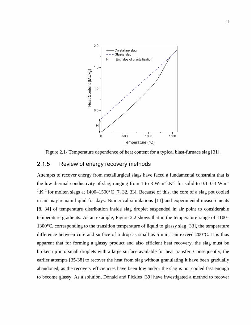
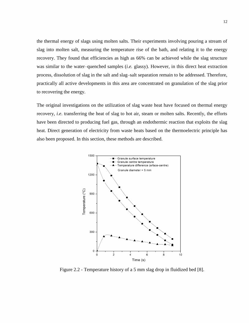
in air may remain liquid for days. Numerical simulations [11] and experimental measurements

[8, 34] of temperature distribution inside slag droplet suspended in air point to considerable

temperature gradients. As an example, Figure 2.2 shows that in the temperature range of 1100–

1300°C, corresponding to the transition temperature of liquid to glassy slag [33], the temperature

difference between core and surface of a drop as small as 5 mm, can exceed 200°C. It is thus

apparent that for forming a glassy product and also efficient heat recovery, the slag must be

broken up into small droplets with a large surface available for heat transfer. Consequently, the

earlier attempts [35-38] to recover the heat from slag without granulating it have been gradually

abandoned, as the recovery efficiencies have been low and/or the slag is not cooled fast enough

to become glassy. As a solution, Donald and Pickles [39] have investigated a method to recover

12

the thermal energy of slags using molten salts. Their experiments involving pouring a stream of

slag into molten salt, measuring the temperature rise of the bath, and relating it to the energy

recovery. They found that efficiencies as high as 66% can be achieved while the slag structure

was similar to the water–quenched samples (i.e. glassy). However, in this direct heat extraction

process, dissolution of slag in the salt and slag–salt separation remain to be addressed. Therefore,

practically all active developments in this area are concentrated on granulation of the slag prior

to recovering the energy.

The original investigations on the utilization of slag waste heat have focused on thermal energy

recovery, i.e. transferring the heat of slag to hot air, steam or molten salts. Recently, the efforts

have been directed to producing fuel gas, through an endothermic reaction that exploits the slag

heat. Direct generation of electricity from waste heats based on the thermoelectric principle has

also been proposed. In this section, these methods are described.

Figure 2.2 - Temperature history of a 5 mm slag drop in fluidized bed [8].

13

Thermal energy recovery

The differences between various methods are in the way slag is fragmented (the use of

centrifugal force or impinging jets), the heat transfer medium (air, steam, or salt), and the heat

transfer mode (i.e. direct–contact in packed or fluidized bed or indirect heat exchange). In this

thesis, the energy recovery methods are categorized based on the method of slag granulation.

A) Rotary cup atomizer (RCA)

The rotary cup atomizer was first designed in Britain by Pickering et al. [31] and has been

extensively studied since then. It essentially atomizes the molten slag by combined actions of a

rotating cup and air blast, and cools the droplets rapidly to produce a glassy product. The

particles are cooled as they travel through air and are later introduced to two successive fluidized

beds for heat recovery. The suspension of particles with mean diameter of 2 mm in fluidized bed

prevents the slag particles from clustering and at the same time provides rapid cooling to

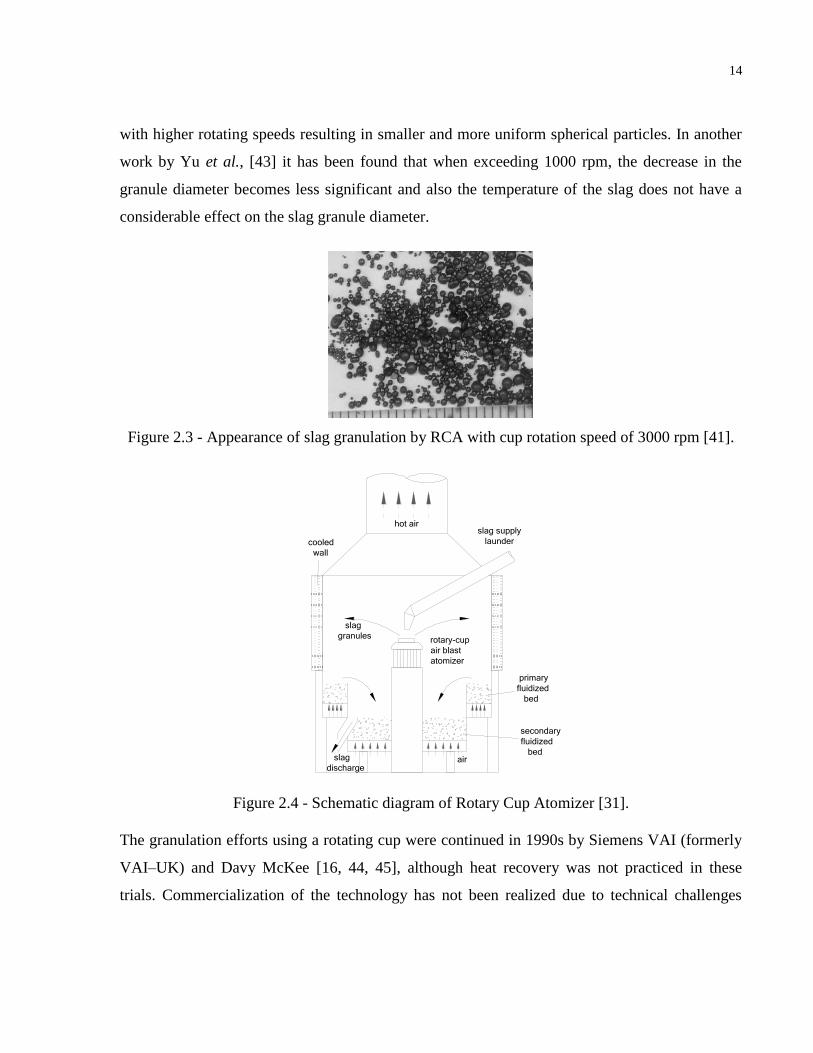
generate slag with over 95% glass content. A schematic diagram of the RCA is presented in

Figure 2.4. It has been discussed that while the fast rotation of the RCA at 500–1500 rpm is

sufficient to generate and break up the slag film, the annular air jet supplied around the cup

facilitates the formation of smaller and more uniform particles. Based on their small scale

experiments (0.2–0.5 kg slag per second), Pickering et al. proposed a commercial scale system,

that if operated continuously, would yield an energy recovery of 59%. The losses occur because

a) the total latent heat is not released when glassy slag is formed b) the solid slag is discharged

from the heat recovery vessel at 250°C and c) heat loss in the slag accumulator. On the other

hand, the main advantages of RCA are claimed to be high productivity and controllable slag

grain diameter Figure 2.3. It has also been proposed by Akiyama and his co–workers [40-42] that

by impinging reactive gas such as mixture of methane and stream, the sensible heat of the slag

can be efficiently recovered as chemical energy as will be explained later.

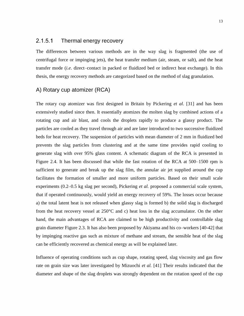
Influence of operating conditions such as cup shape, rotating speed, slag viscosity and gas flow

rate on grain size was later investigated by Mizuochi et al. [41] Their results indicated that the

diameter and shape of the slag droplets was strongly dependent on the rotation speed of the cup

14

with higher rotating speeds resulting in smaller and more uniform spherical particles. In another

work by Yu et al., [43] it has been found that when exceeding 1000 rpm, the decrease in the

granule diameter becomes less significant and also the temperature of the slag does not have a

considerable effect on the slag granule diameter.

Figure 2.3 - Appearance of slag granulation by RCA with cup rotation speed of 3000 rpm [41].

Figure 2.4 - Schematic diagram of Rotary Cup Atomizer [31].

The granulation efforts using a rotating cup were continued in 1990s by Siemens VAI (formerly

VAI–UK) and Davy McKee [16, 44, 45], although heat recovery was not practiced in these

trials. Commercialization of the technology has not been realized due to technical challenges

hot air

cooled

wall

primary

fluidized

bed

secondary

fluidized

bed

slag

granulesrotary-cup

air blast

atomizer

slag

dischargeair

slag supply

launder

15

such as formation of slag wool and degradation of the atomizer cup. Recently, rotary cylinder

has been tested in the laboratory scale [46], anticipating a higher efficiency of the granulation

energy due to the reduced slip between slag and metal in this design. The experiments have

shown that spherical glassy slag of various sizes can be produced, however, heat recovery tests

have not been performed.

B) Granulation by spinning disk

The early works involved the use of spinning disks for slag granulation were carried out in Japan

by Sumitomo Metal Industries in 1980s [8], aiming to form a BF glassy slag. Recent

developments in spinning disk granulation method include the works of Akiyama and co–

workers at Hokkaido University, Japan, [40, 41, 47], and those of Xie, et al. [23, 24, 48-50] at

CSIRO, Australia. The former group however have proposed the recovery of the slag heat into

chemical energy, as will be explained later.

In spinning disk granulation, a stream of slag is delivered onto the disk rotating at 1000–3000

rpm. The liquid steam is fragmented due to the impact with the disk and the centrifugal force.

The droplets are scattered radially and collected in the heat recovery chamber where slag is

cooled in fluidized or packed bed.

CSIRO has been working on the design, development and scale up of the method since 2002

[48]. The early works involved optimization of the granulation method that was later integrated

with heat recovery. Their concept is based on a two–step process; in the first step, molten slag is

granulated using the spinning disk. Through contact with an uprising air flow, the slag droplets

freeze and their temperature drops to about 900°C, forming an amorphous phase. This slag is

then charged to a packed bed heat exchanger where counter–current flow of secondary air cools

the slag to about 50°C. The hot air of both steps is at temperatures above 600°C and may be used

to generate steam or be used for preheating/drying.

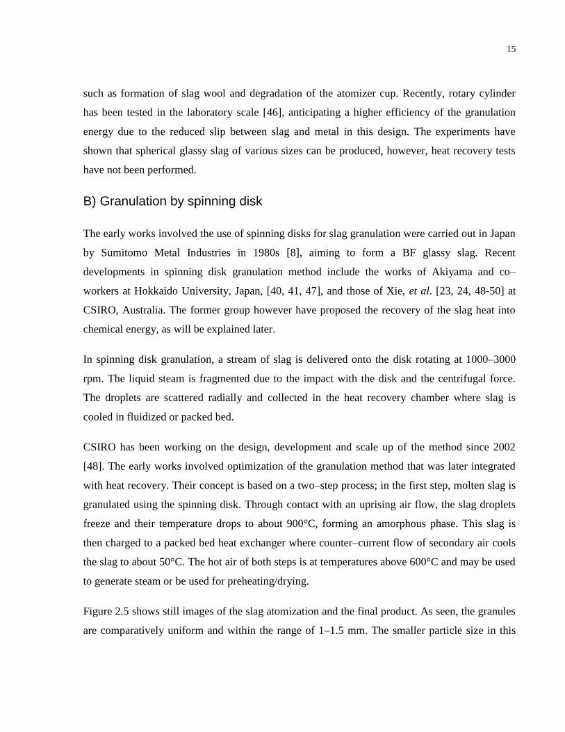
Figure 2.5 shows still images of the slag atomization and the final product. As seen, the granules

are comparatively uniform and within the range of 1–1.5 mm. The smaller particle size in this

16

technology offers several advantages, including faster cooling, higher glassy content, shorter

flight time, and ease of grinding for subsequent use.

Figure 2.5 - (a) slag atomization on the spinning disc and (b) granulated slag product [23, 50].

Their process has been successfully tested on blast furnace slag at rates up to 10 kg/min. Further

developments are underway to first test slag rates up to 100 kg/min and later 1000–2000 kg/min.

C) Granulation using rotating drum

In early 80s, Japanese companies Ishikawajima–Harima Heavy Industries and Sumitomo Metal

developed a process in which a stream of blast furnace slag breaks up as it is impinged onto a

rotating drum [13, 51-53]. The slag particles then fall into a fluidized bed where the heat was

recovered. The process was later modified to lubricate the drum surface with a thin film of water

or oil, giving rise to smaller heat loss and reduction in the particles scattering [8]. Further,

pulverized cool slag was injected into the fluidized bed to accelerate the slag cooling, in order to

decrease the required flight time for the droplets and make the plant smaller [8]. It also reduces

the agglomeration of slag particles at high temperature. This process was tested in full scale of

40 t/hr at Wakayama Steel Works [8, 13] with a reported 50–60 % recovery of the slag sensible

heat into hot air. A flowsheet of the process is provided in Figure 2.6.

17

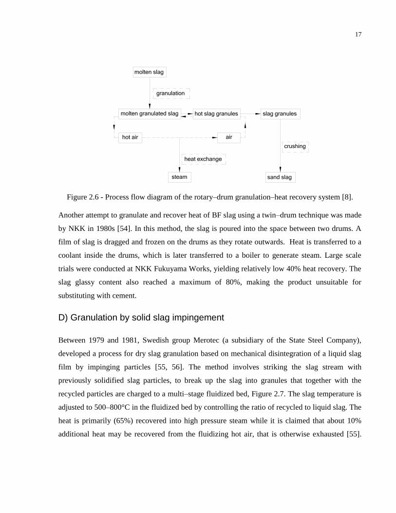
Figure 2.6 - Process flow diagram of the rotary–drum granulation–heat recovery system [8].

Another attempt to granulate and recover heat of BF slag using a twin–drum technique was made

by NKK in 1980s [54]. In this method, the slag is poured into the space between two drums. A

film of slag is dragged and frozen on the drums as they rotate outwards. Heat is transferred to a

coolant inside the drums, which is later transferred to a boiler to generate steam. Large scale

trials were conducted at NKK Fukuyama Works, yielding relatively low 40% heat recovery. The

slag glassy content also reached a maximum of 80%, making the product unsuitable for

substituting with cement.

D) Granulation by solid slag impingement

Between 1979 and 1981, Swedish group Merotec (a subsidiary of the State Steel Company),

developed a process for dry slag granulation based on mechanical disintegration of a liquid slag

film by impinging particles [55, 56]. The method involves striking the slag stream with

previously solidified slag particles, to break up the slag into granules that together with the

recycled particles are charged to a multi–stage fluidized bed, Figure 2.7. The slag temperature is

adjusted to 500–800°C in the fluidized bed by controlling the ratio of recycled to liquid slag. The

heat is primarily (65%) recovered into high pressure steam while it is claimed that about 10%

additional heat may be recovered from the fluidizing hot air, that is otherwise exhausted [55].

molten slag

granulation

molten granulated slag hot slag granules

airhot air

heat exchange

slag granules

crushing

sand slagsteam

18

The slag granulates are typically below 6 mm where the –3 mm particles are recycled to the

granulator.

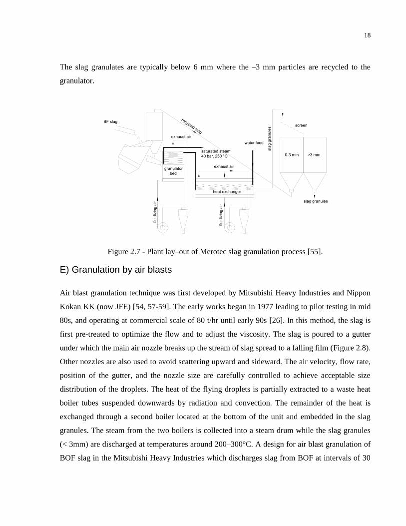
Figure 2.7 - Plant lay–out of Merotec slag granulation process [55].

E) Granulation by air blasts

Air blast granulation technique was first developed by Mitsubishi Heavy Industries and Nippon

Kokan KK (now JFE) [54, 57-59]. The early works began in 1977 leading to pilot testing in mid

80s, and operating at commercial scale of 80 t/hr until early 90s [26]. In this method, the slag is

first pre-treated to optimize the flow and to adjust the viscosity. The slag is poured to a gutter

under which the main air nozzle breaks up the stream of slag spread to a falling film (Figure 2.8).

Other nozzles are also used to avoid scattering upward and sideward. The air velocity, flow rate,

position of the gutter, and the nozzle size are carefully controlled to achieve acceptable size

distribution of the droplets. The heat of the flying droplets is partially extracted to a waste heat

boiler tubes suspended downwards by radiation and convection. The remainder of the heat is

exchanged through a second boiler located at the bottom of the unit and embedded in the slag

granules. The steam from the two boilers is collected into a steam drum while the slag granules

(< 3mm) are discharged at temperatures around 200–300°C. A design for air blast granulation of

BOF slag in the Mitsubishi Heavy Industries which discharges slag from BOF at intervals of 30

BF slagrecycled slag

granulator

bed

saturated steam

40 bar, 250 C

water feed

sla

g g

ran

ule

s screen

0-3 mm >3 mm

slag granules

flu

idiz

ing

air

flu

idiz

ing

air

exhaust air

exhaust air

heat exchanger

19

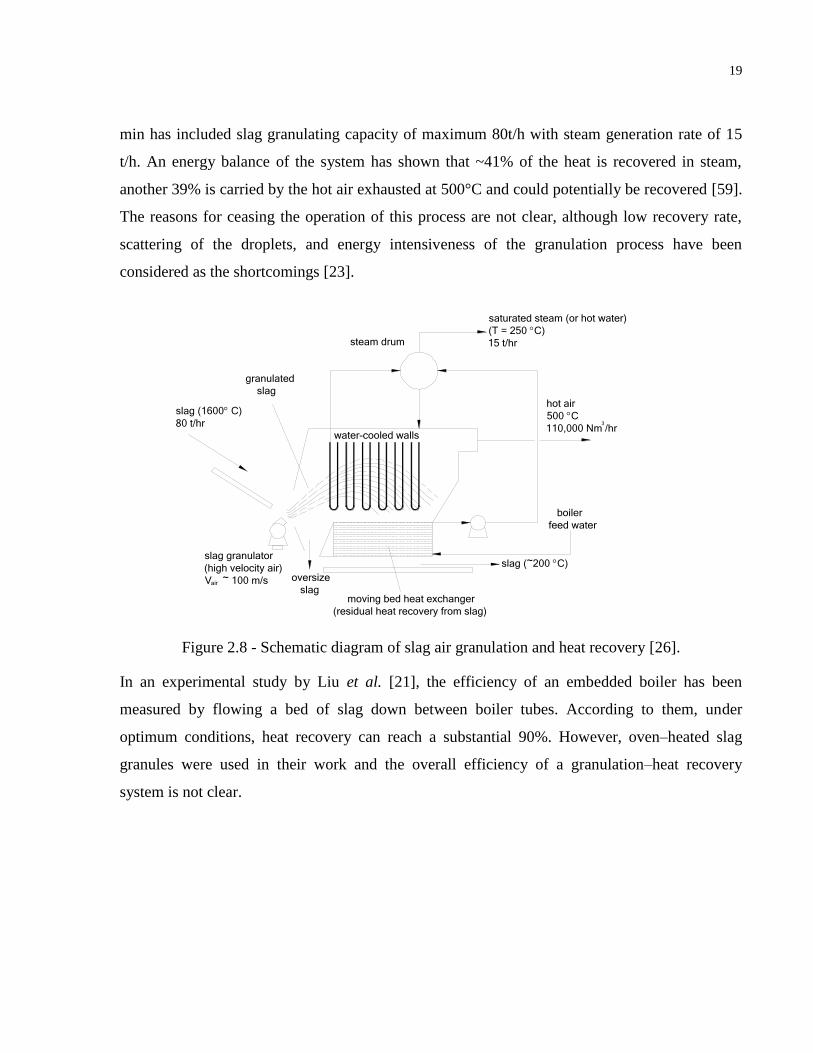
min has included slag granulating capacity of maximum 80t/h with steam generation rate of 15

t/h. An energy balance of the system has shown that ~41% of the heat is recovered in steam,

another 39% is carried by the hot air exhausted at 500°C and could potentially be recovered [59].

The reasons for ceasing the operation of this process are not clear, although low recovery rate,

scattering of the droplets, and energy intensiveness of the granulation process have been

considered as the shortcomings [23].

Figure 2.8 - Schematic diagram of slag air granulation and heat recovery [26].

In an experimental study by Liu et al. [21], the efficiency of an embedded boiler has been

measured by flowing a bed of slag down between boiler tubes. According to them, under

optimum conditions, heat recovery can reach a substantial 90%. However, oven–heated slag

granules were used in their work and the overall efficiency of a granulation–heat recovery

system is not clear.

oversize

slag

slag (1600C)

80 t/hr

steam drum

granulated

slag

moving bed heat exchanger

(residual heat recovery from slag)

boiler

feed water

water-cooled walls

saturated steam (or hot water)

(T = 250 C)

15 t/hr

slag (~200 C)

hot air

500 C

110,000 Nm /hr 3

slag granulator

(high velocity air)

V ~ 100 m/sair

20

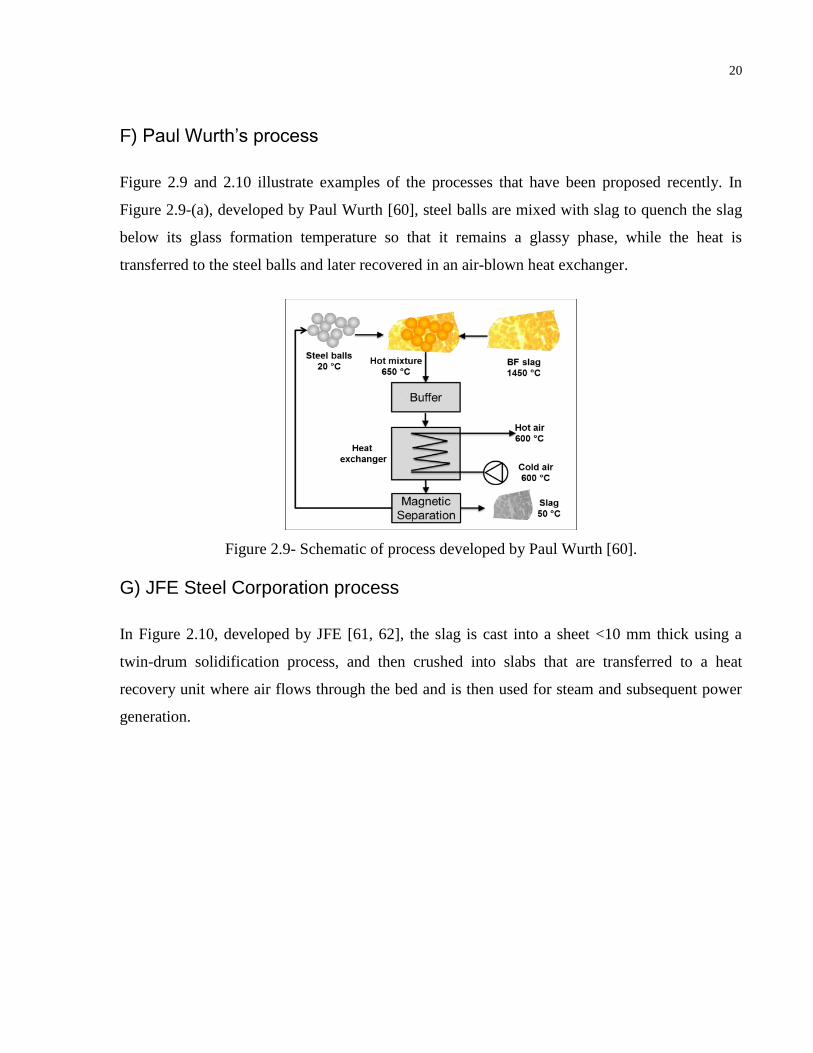
F) Paul Wurth’s process

Figure 2.9 and 2.10 illustrate examples of the processes that have been proposed recently. In

Figure 2.9-(a), developed by Paul Wurth [60], steel balls are mixed with slag to quench the slag

below its glass formation temperature so that it remains a glassy phase, while the heat is

transferred to the steel balls and later recovered in an air-blown heat exchanger.

Figure 2.9- Schematic of process developed by Paul Wurth [60].

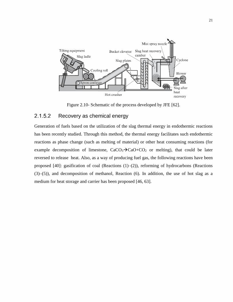
G) JFE Steel Corporation process

In Figure 2.10, developed by JFE [61, 62], the slag is cast into a sheet <10 mm thick using a

twin-drum solidification process, and then crushed into slabs that are transferred to a heat

recovery unit where air flows through the bed and is then used for steam and subsequent power

generation.

21

Figure 2.10- Schematic of the process developed by JFE [62].

Recovery as chemical energy

Generation of fuels based on the utilization of the slag thermal energy in endothermic reactions

has been recently studied. Through this method, the thermal energy facilitates such endothermic

reactions as phase change (such as melting of material) or other heat consuming reactions (for

example decomposition of limestone, CaCO3CaO+CO2 or melting), that could be later

reversed to release heat. Also, as a way of producing fuel gas, the following reactions have been

proposed [40]: gasification of coal (Reactions (1)–(2)), reforming of hydrocarbons (Reactions

(3)–(5)), and decomposition of methanol, Reaction (6). In addition, the use of hot slag as a

medium for heat storage and carrier has been proposed [46, 63].

22

Table 2.4- Endothermic reactions for chemical recovery of waste heats [40].

Reaction Enthalpy

(kJ/mol)

Exergy

(kJ/mol)

(1)

𝐶 + 𝐶𝑂2 → 2𝐶𝑂

172

122

(2)

𝐶 + 𝐻2𝑂 → 𝐶𝑂 + 𝐻2

131

91

(3)

𝐶𝐻4 + 𝐶𝑂2 → 2 𝐶𝑂 + 2𝐻2

247

171

(4)

𝐶𝐻4 + 𝐻2𝑂 → 𝐶𝑂 + 3𝐻2

206

142

(5)

𝐶𝐻8 + 𝐻2𝑂 → 𝐶𝑂 + 5𝐻2

498

298

(6)

𝐶𝐻3𝑂𝐻 → 𝐶𝑂 + 2𝐻2

90

25

Table 2.4 summarizes the proposed endothermic reactions and their thermodynamic data. An

analysis [40] of the reactions has shown that decomposition of limestone, reforming of methane,

and gasification of carbon are the most promising heat absorbing reactions, as they present the

least exergy loss among all the reactions studied. The latter two processes have received more

attention due to their potential to generate fuel that is easy to transport and be used for various

applications.

A) Energy recovery by methane reforming

In 1997 Kasai et al. [42] proposed the use of hot BF slag for promoting water reforming of

methane (i.e. Reaction (4)). Figure 2.11 depicts the scheme of this concept. As shown, part of the

slag sensible heat is transferred to the reactants (methane and steam), generating CO and H2. The

still molten slag (~ 1500 K) is transferred to the granulation step, in which steam is generated by

extracting the remainder of the sensible and latent heat. The steam is fed back to the reformer,

thereby increasing the overall efficiency of the process. The sensible heat of the high temperature

reducing gases is recovered through a heat exchanger that produces steam for power generation.

The chemical energy of the gases is partially recovered in the methanation reactor where the

reverse reaction generates methane and steam. Water vapor is condensed in a second heat

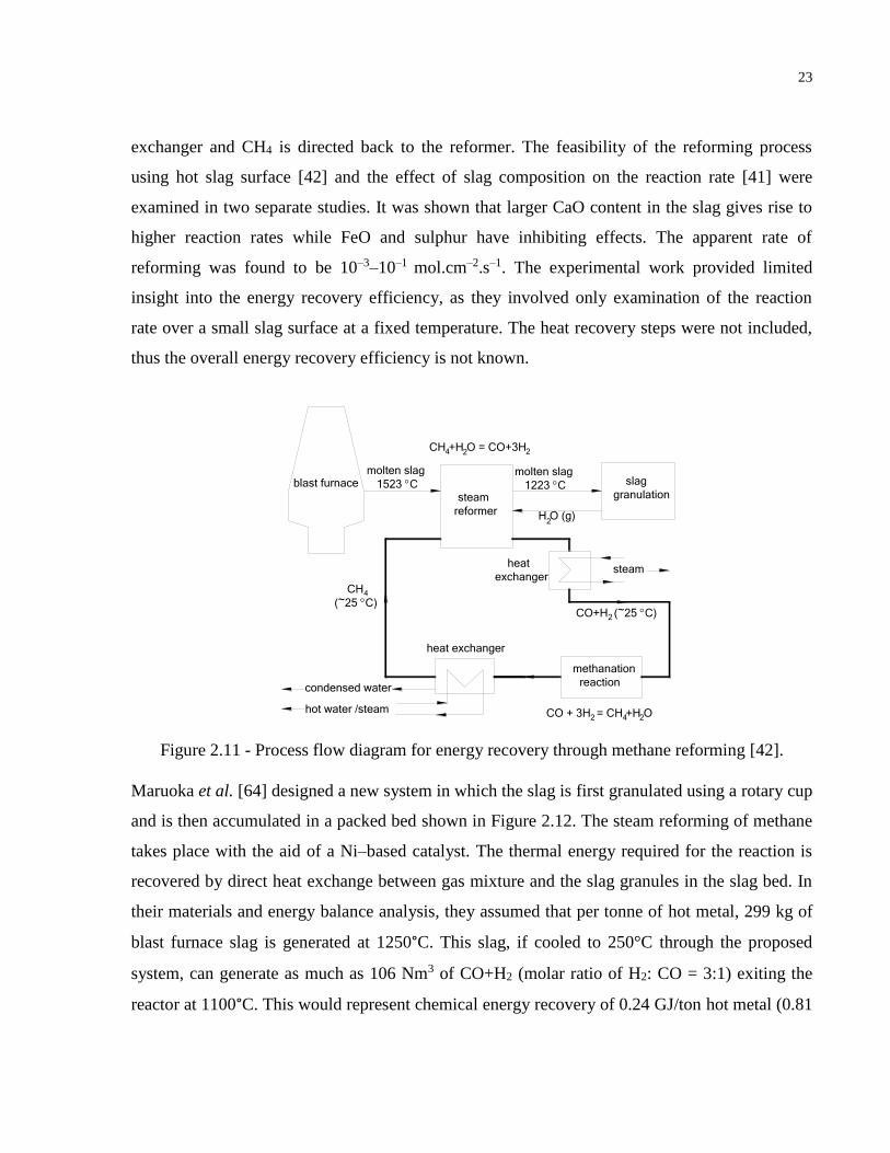
23

exchanger and CH4 is directed back to the reformer. The feasibility of the reforming process

using hot slag surface [42] and the effect of slag composition on the reaction rate [41] were

examined in two separate studies. It was shown that larger CaO content in the slag gives rise to

higher reaction rates while FeO and sulphur have inhibiting effects. The apparent rate of

reforming was found to be 10–3–10–1 mol.cm–2.s–1. The experimental work provided limited

insight into the energy recovery efficiency, as they involved only examination of the reaction

rate over a small slag surface at a fixed temperature. The heat recovery steps were not included,

thus the overall energy recovery efficiency is not known.

Figure 2.11 - Process flow diagram for energy recovery through methane reforming [42].

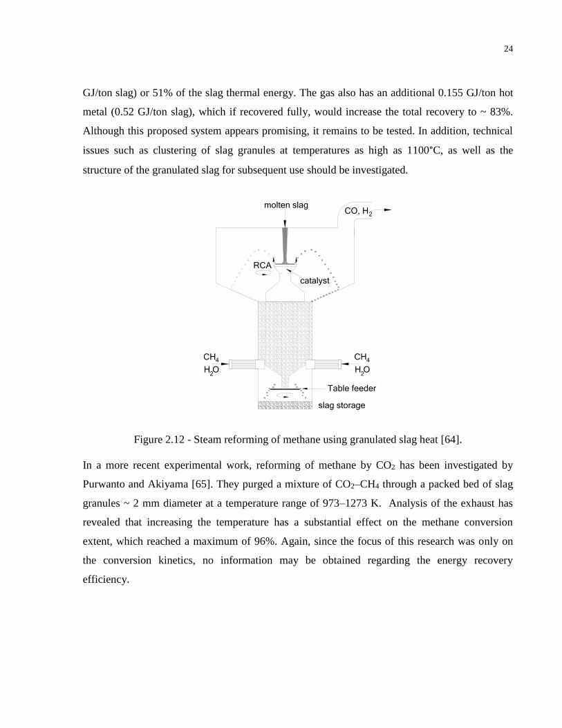
Maruoka et al. [64] designed a new system in which the slag is first granulated using a rotary cup

and is then accumulated in a packed bed shown in Figure 2.12. The steam reforming of methane

takes place with the aid of a Ni–based catalyst. The thermal energy required for the reaction is

recovered by direct heat exchange between gas mixture and the slag granules in the slag bed. In

their materials and energy balance analysis, they assumed that per tonne of hot metal, 299 kg of

blast furnace slag is generated at 1250°C. This slag, if cooled to 250°C through the proposed

system, can generate as much as 106 Nm3 of CO+H2 (molar ratio of H2: CO = 3:1) exiting the

reactor at 1100°C. This would represent chemical energy recovery of 0.24 GJ/ton hot metal (0.81

blast furnace

steam

reformer

slag

granulation

steam

methanation

reaction

CO + 3H = CH +H O

heat exchanger

hot water /steam

CH

(~25 C)

H O (g)

heat

exchanger

2

CO+H (~25 C)2

2 4 2

4

CH +H O = CO+3H24 2

condensed water

molten slag

1223 C

molten slag

1523 C

24

GJ/ton slag) or 51% of the slag thermal energy. The gas also has an additional 0.155 GJ/ton hot

metal (0.52 GJ/ton slag), which if recovered fully, would increase the total recovery to ~ 83%.

Although this proposed system appears promising, it remains to be tested. In addition, technical

issues such as clustering of slag granules at temperatures as high as 1100°C, as well as the

structure of the granulated slag for subsequent use should be investigated.

Figure 2.12 - Steam reforming of methane using granulated slag heat [64].

In a more recent experimental work, reforming of methane by CO2 has been investigated by

Purwanto and Akiyama [65]. They purged a mixture of CO2–CH4 through a packed bed of slag

granules ~ 2 mm diameter at a temperature range of 973–1273 K. Analysis of the exhaust has

revealed that increasing the temperature has a substantial effect on the methane conversion

extent, which reached a maximum of 96%. Again, since the focus of this research was only on

the conversion kinetics, no information may be obtained regarding the energy recovery

efficiency.

CH

2

4

H O

CH

2

4

H O

Table feeder

catalyst

RCA

CO, H 2molten slag

slag storage

25

Converting the thermal energy to chemical energy, particularly in the form of a fuel, offers

advantages such as a higher energy density (compared to steam/hot air), possibility of

transporting energy, and the potential of re-generating the thermal energy at much greater

temperatures. However, an analysis by the author shows that the rate of heat extraction from slag

by such reactions as methane reforming is far from being enough to prevent the slag from

crystallization. According to Sun et al.[66], this can be addressed by converting the thermal

energy of slag to chemical energy only when the slag temperature is below the glass formation

temperature, so that extended periods do not result in crystallization of slag. In other words, the

energy recovery process will consist of at least two steps, one for the high temperature range,

where slag needs to be cooled rapidly, perhaps using air, and the second step in which slag is

cooled through endothermic reactions. For this purpose, the crystallization behavior of the slag at

different temperatures needs to be established.

B) Energy recovery by coal gasification

In a study by Li et al. [40], recovering slag heat through coal gasification was evaluated by using

a materials–energy balance. In the proposed coal gasification system, CO2 is injected together

with coal into a molten BF slag bath, generating carbon monoxide through Reaction (1). The

thermal energy of off–gas is recovered in a heat exchanger to make steam while the cleaned gas

is used as fuel. According to this analysis, a steel mill generating 10 Mt of steel would also

produce 3 Mt slag, from which 0.132 Mt of CO is generated. Based on energy content of 1.6

GJ/ton slag, this represents thermal–to–chemical conversion efficiency of 35%. However, the

total energy recovery is greater, because a non–quantified amount of heat is recovered as steam.

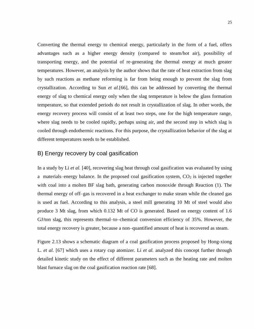
Figure 2.13 shows a schematic diagram of a coal gasification process proposed by Hong-xiong

L. et al. [67] which uses a rotary cup atomizer. Li et al. analyzed this concept further through

detailed kinetic study on the effect of different parameters such as the heating rate and molten

blast furnace slag on the coal gasification reaction rate [68].

26

Figure 2.13 – Coal gasification process [67].

C) Energy recovery through PCB (Printed Circuit Boards)

In a recent investigation by Qin et al. [67] a new technique was proposed which recovers the heat

of BF slag by first granulating slag using rotary a multinozzle cup atomizer and later pyrolyzing

printed circuited boards.

Direct electricity generation

Direct conversion of waste heat to thermoelectric power has been recently reviewed by Rowe

[69]. The method presents an environmentally friendly, safe and reliable technology which can

convert unused heat into electricity. With the emergence of modern semiconductors with

Seebeck coefficient in the order of several hundred microvolts per degree, the technology

appears promising, particularly for high quality heat such as that of slag. Low temperature trials

have been successfully demonstrated on a laboratory scale and in prototype commercial systems.

As an example, an investigation on steel plant heat recovery has been carried out where large

amounts of cooling water are discharged at constant temperatures of around 90°C. It has been

estimated that total electrical power of around 8 MW would be produced employing currently

available modules fabricated using bismuth telluride material technology.

27

The thermoelectric technology is an emerging area, particularly for high temperature

applications. The choice of thermoelectric materials with large Seebeck coefficient for high

temperature systems is rather limited. However, the slag waste heat may be stored in phase

change materials (PCMs) as proposed by Nomura et al.[63], in a temperature range of ~150–

1000°C, coinciding well with the operating temperature for a range of thermoelectric materials

that may suitably be used for energy conversion.

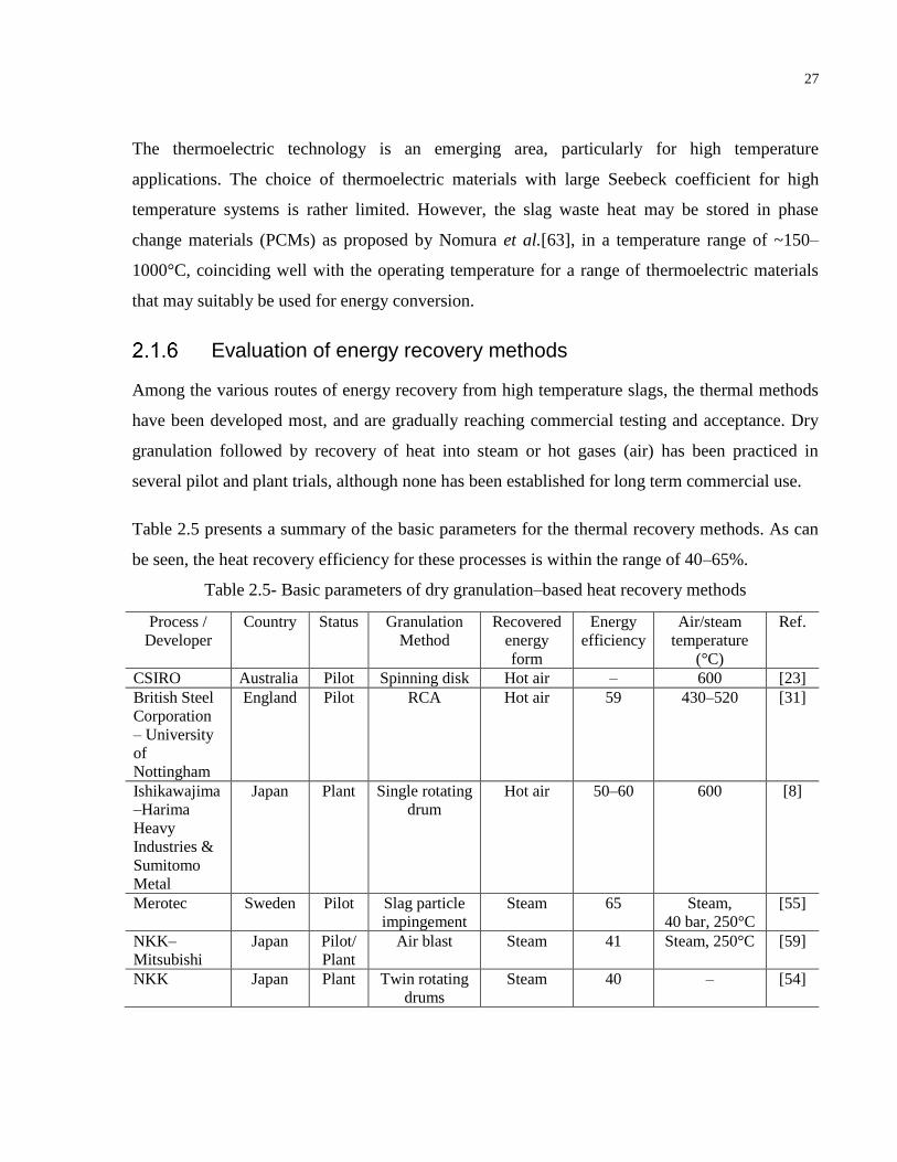
Evaluation of energy recovery methods

Among the various routes of energy recovery from high temperature slags, the thermal methods

have been developed most, and are gradually reaching commercial testing and acceptance. Dry

granulation followed by recovery of heat into steam or hot gases (air) has been practiced in

several pilot and plant trials, although none has been established for long term commercial use.

Table 2.5 presents a summary of the basic parameters for the thermal recovery methods. As can

be seen, the heat recovery efficiency for these processes is within the range of 40–65%.

Table 2.5- Basic parameters of dry granulation–based heat recovery methods

Process /

Developer

Country Status Granulation

Method

Recovered

energy

form

Energy

efficiency

Air/steam

temperature

(°C)

Ref.

CSIRO Australia Pilot Spinning disk Hot air – 600 [23]

British Steel

Corporation

– University

of

Nottingham

England Pilot RCA Hot air 59 430–520 [31]

Ishikawajima

–Harima

Heavy

Industries &

Sumitomo

Metal

Japan Plant Single rotating

drum

Hot air 50–60 600 [8]

Merotec Sweden Pilot Slag particle

impingement

Steam 65 Steam,

40 bar, 250°C

[55]

NKK–

Mitsubishi

Japan Pilot/

Plant

Air blast Steam 41 Steam, 250°C [59]

NKK Japan Plant Twin rotating

drums

Steam 40 – [54]

28

The requirement for forming a glassy product while recovering the heat poses a fundamental

challenge in efficient heat recovery. While large quantities of air are required for rapid

quenching of solidifying slag, the temperature (and heat quality) of the heat carrier, steam/air, is

reduced at higher flow rate. The lower gas temperature in turn reduces the recovery of energy

utilization as steam or heat source in the subsequent steps, leading to lower overall efficiency. As

a result, the trend in the slag treatment processes is towards controlled granulation so that small

and uniform slag grains are generated. The larger contact area promotes heat transfer for a given

air flow rate, and also facilitates fluidization of the grains, as well as their subsequent use as

cement feedstock. In addition, Bisio [70] has shown that where the use for hot air exists, such as

blast furnace, generation of hot air is more energy efficient than steam.

The recovery of heat from dry–granulated slag grains conventionally takes place in fluidized bed

for improved heat transfer and also preventing agglomeration of the particles. However, the

disadvantage of fluid–bed is that slag is discharged at a temperature typically above 200°C,

causing energy loss. An optimum design may include a two–step heat recovery, in which initially

the slag is rapidly cooled in a fluidized bed below the clustering temperature (800–900°C).

Subsequently, the remainder of the heat is recovered in a packed bed, through embedded boiler

tubes or direct contact of air–slag. Within this context, the proposed process by CSIRO [23, 48,

50] appears very promising, as the slag discharge temperature (50°C) is considerably lower than

the previous methods (~200–300°C). Such difference in the slag temperature could result in

increasing the recovery efficiency by additional 10–15% compared to those presented in Table

2.5.

Conversion of slag waste heat into chemical energy offers several advantages over the thermal

technologies:

1. The fuel may be transported over long distances without a loss in the energy content.

2. Metallurgical industry may be linked to the chemical and energy sectors.

3. Fuels have a substantially larger energy density compared to steam or hot air, making

their transportation and storage more economically attractive. As an example, the energy

density of saturated steam at 250°C (40 bar) is 44 MJ/m3, whereas that of CO–H2 gas

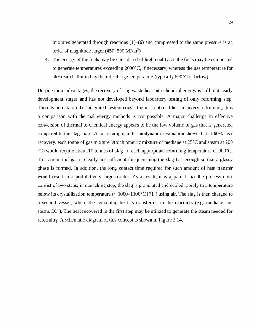
29

mixtures generated through reactions (1)–(6) and compressed to the same pressure is an

order of magnitude larger (450–500 MJ/m3).

4. The energy of the fuels may be considered of high quality, as the fuels may be combusted

to generate temperatures exceeding 2000°C, if necessary, whereas the use temperature for

air/steam is limited by their discharge temperature (typically 600°C or below).

Despite these advantages, the recovery of slag waste heat into chemical energy is still in its early

development stages and has not developed beyond laboratory testing of only reforming step.

There is no data on the integrated system consisting of combined heat recovery–reforming, thus

a comparison with thermal energy methods is not possible. A major challenge in effective

conversion of thermal to chemical energy appears to be the low volume of gas that is generated

compared to the slag mass. As an example, a thermodynamic evaluation shows that at 60% heat

recovery, each tonne of gas mixture (stoichiometric mixture of methane at 25°C and steam at 200

°C) would require about 10 tonnes of slag to reach appropriate reforming temperature of 900°C.

This amount of gas is clearly not sufficient for quenching the slag fast enough so that a glassy

phase is formed. In addition, the long contact time required for such amount of heat transfer

would result in a prohibitively large reactor. As a result, it is apparent that the process must

consist of two steps; in quenching step, the slag is granulated and cooled rapidly to a temperature

below its crystallization temperature (~ 1000–1100°C [71]) using air. The slag is then charged to

a second vessel, where the remaining heat is transferred to the reactants (e.g. methane and

steam/CO2). The heat recovered in the first step may be utilized to generate the steam needed for

reforming. A schematic diagram of this concept is shown in Figure 2.14.

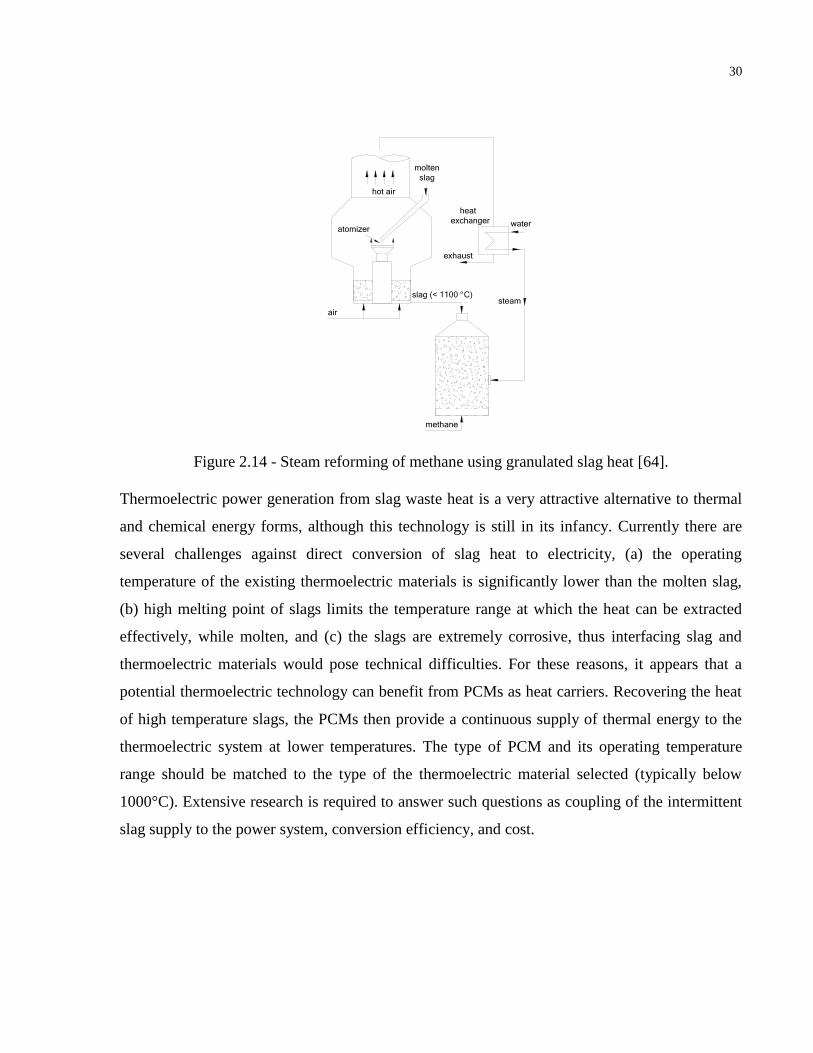
30

Figure 2.14 - Steam reforming of methane using granulated slag heat [64].

Thermoelectric power generation from slag waste heat is a very attractive alternative to thermal

and chemical energy forms, although this technology is still in its infancy. Currently there are

several challenges against direct conversion of slag heat to electricity, (a) the operating

temperature of the existing thermoelectric materials is significantly lower than the molten slag,

(b) high melting point of slags limits the temperature range at which the heat can be extracted

effectively, while molten, and (c) the slags are extremely corrosive, thus interfacing slag and

thermoelectric materials would pose technical difficulties. For these reasons, it appears that a

potential thermoelectric technology can benefit from PCMs as heat carriers. Recovering the heat

of high temperature slags, the PCMs then provide a continuous supply of thermal energy to the

thermoelectric system at lower temperatures. The type of PCM and its operating temperature

range should be matched to the type of the thermoelectric material selected (typically below

1000°C). Extensive research is required to answer such questions as coupling of the intermittent

slag supply to the power system, conversion efficiency, and cost.

atomizer

molten

slag

hot air

air

heat

exchanger water

steam

methane

slag (< 1100 C)

exhaust

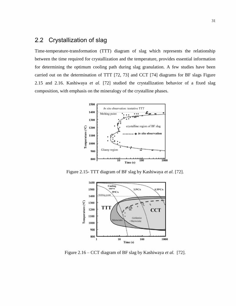
31

Crystallization of slag

Time-temperature-transformation (TTT) diagram of slag which represents the relationship

between the time required for crystallization and the temperature, provides essential information

for determining the optimum cooling path during slag granulation. A few studies have been

carried out on the determination of TTT [72, 73] and CCT [74] diagrams for BF slags Figure

2.15 and 2.16. Kashiwaya et al. [72] studied the crystallization behavior of a fixed slag

composition, with emphasis on the mineralogy of the crystalline phases.

Figure 2.15- TTT diagram of BF slag by Kashiwaya et al. [72].

Figure 2.16 – CCT diagram of BF slag by Kashiwaya et al. [72].

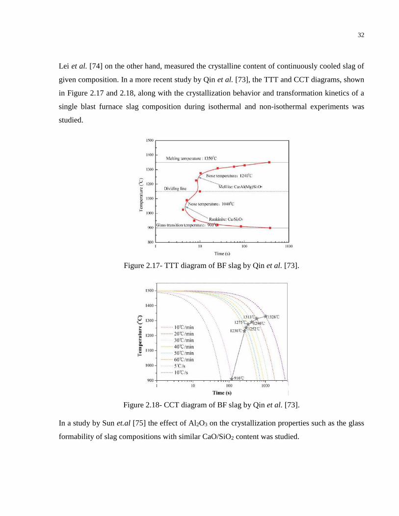
32

Lei et al. [74] on the other hand, measured the crystalline content of continuously cooled slag of

given composition. In a more recent study by Qin et al. [73], the TTT and CCT diagrams, shown

in Figure 2.17 and 2.18, along with the crystallization behavior and transformation kinetics of a

single blast furnace slag composition during isothermal and non-isothermal experiments was

studied.

Figure 2.17- TTT diagram of BF slag by Qin et al. [73].

Figure 2.18- CCT diagram of BF slag by Qin et al. [73].

In a study by Sun et.al [75] the effect of Al2O3 on the crystallization properties such as the glass

formability of slag compositions with similar CaO/SiO2 content was studied.

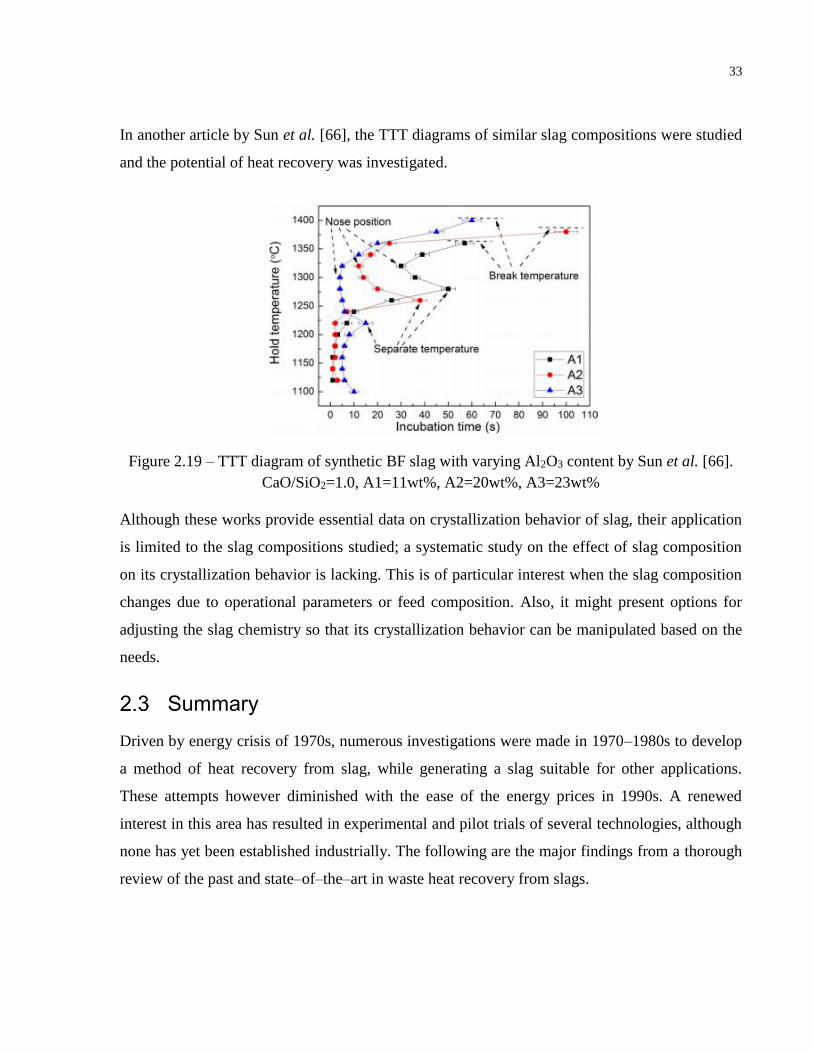
33

In another article by Sun et al. [66], the TTT diagrams of similar slag compositions were studied

and the potential of heat recovery was investigated.

Figure 2.19 – TTT diagram of synthetic BF slag with varying Al2O3 content by Sun et al. [66].

CaO/SiO2=1.0, A1=11wt%, A2=20wt%, A3=23wt%

Although these works provide essential data on crystallization behavior of slag, their application

is limited to the slag compositions studied; a systematic study on the effect of slag composition

on its crystallization behavior is lacking. This is of particular interest when the slag composition

changes due to operational parameters or feed composition. Also, it might present options for

adjusting the slag chemistry so that its crystallization behavior can be manipulated based on the

needs.

Summary

Driven by energy crisis of 1970s, numerous investigations were made in 1970–1980s to develop

a method of heat recovery from slag, while generating a slag suitable for other applications.

These attempts however diminished with the ease of the energy prices in 1990s. A renewed

interest in this area has resulted in experimental and pilot trials of several technologies, although

none has yet been established industrially. The following are the major findings from a thorough

review of the past and state–of–the–art in waste heat recovery from slags.

34

1. The world production of slag represents a heat content of 282 TWh per year (2013), with

blast furnace slag accounting for about 50% of this energy.

2. Driven by a demand to produce amorphous slag as substitute to cement and limited by

the low thermal conductivity of slag, majority of the methods for energy recovery from

slag are relying on dry granulation of slag.

3. Being investigated for over three decades, the thermal energy recovery methods are most

developed among the various schemes proposed for energy recovery from slags.

4. Compared to rotary drum or air jet granulation, the techniques employing spinning disks

or rotary cups offer the advantage of generating uniform and small grains at a lower

energy consumption rate. Smaller droplets are quenched faster and require less coolant,

resulting in recovery of more heat and at higher temperature.

5. Because of the cooling rate requirements, a two–step heat recovery consisting of a

fluidized bed, followed by a packed bed would yield higher energy recovery efficiency,

as both high outlet gas temperature and low slag discharge temperature are achieved.

6. The chemical energy recovery methods offer the advantage of high energy density and

zero loss in the energy content during transportation. These methods are under

investigation, with methane reforming and coal gasification receiving more attention as

the feasible routes.

7. An optimum chemical energy recovery system consists of two vessels, where in one the

slag is cooled to below the crystallization temperature, and in the other fuel generation

takes place.

8. Thermoelectric power generation based on the slag waste heat appears to be the next

emerging technology in this area. The use of PCMs as heat carriers appears to address the

major challenges that the technology is currently facing.

9. Currently, substituting Portland cement with slag cement is one of the most desirable uses

of slags. For this application, high cooling rates are required to form an amorphous

(glassy) slag. However, it is crucial to develop an ideal cooling path that prevents crystal

formation and at the same time allows efficient recovery of high quality heat from slag.

35

10. TTT and CCT diagrams are useful tools which can help control and predict the

microstructure of slags and therefore enhance the recycle and reuse of slags. These

findings will not only be interesting from fundamental point of view, they also lead to

possible optimization of the slag chemistry for dictating its crystallization behavior, and

expanding heat recovery options from slag.

11. Although there have been studies on the crystallization behavior of BF slag, their

application is limited to only those slag compositions studied; a systematic study on the

effect of slag composition on its crystallization behavior is lacking.

36

Chapter 3

Experimental

Experiments to study the crystallization behavior of slag were performed by the hot

thermocouple technique. In this chapter first the details of the device functions and the set-up

will be discussed and later the experiments will be explained.

Hot Thermocouple Technique (HTT)

The hot thermocouple technique (HTT) is an experimental method that allows heating, cooling,

or isothermal treatment of materials with precise control of temperature and cooling/heating

rates. The technique relies on the use of a thermocouple wire as both a temperature sensing

device, and a heating element. The specimen under investigation is placed on the tip of the

thermocouple and undergoes the desired thermal treatment. Small sample size allows thermal

homogeneity within the material, also direct contact between the specimen and thermocouple

reduces temperature difference. Further, the specimen can be visualized in-situ throughout the

process, allowing observation of high temperature interactions and phenomena. Rapid

temperature readings followed by current injection to the material in between allow precise

control of the temperature and heating rate.

The hot thermocouple technique has been widely used in studying the effect of composition and

cooling rate on the glass formability and kinetics of crystallization of mold flux. For example,

Kashiwaya et al. [76, 77] and Orrling et al. have studied the crystallization behavior [78, 79] and

the effect of water vapor [80] on the crystallization of mold flux. In two other studies by Klug et

al. [81, 82] the effect of Na2O on fluorine-free mold flux was investigated by plotting the TTT

diagram of the material. Similar studies on mold flux using this technique include the works

reported in References [83-91]. In addition to mold flux, the technique has been employed by

Prapakorn et al. [92] and Valdez et al. [93] to evaluate crystallization behavior of metallurgical

slags. Another example is the research by Jing et al. on Ti-bearing blast furnace slags [94] and

the study by Qin et al. on crystallization behavior and construction of time-temperature-

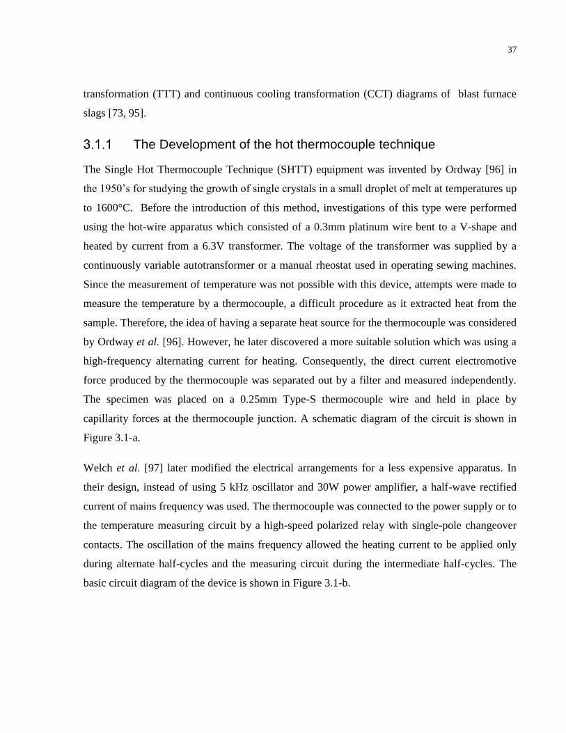
37

transformation (TTT) and continuous cooling transformation (CCT) diagrams of blast furnace

slags [73, 95].

The Development of the hot thermocouple technique

The Single Hot Thermocouple Technique (SHTT) equipment was invented by Ordway [96] in

the 1950’s for studying the growth of single crystals in a small droplet of melt at temperatures up

to 1600°C. Before the introduction of this method, investigations of this type were performed

using the hot-wire apparatus which consisted of a 0.3mm platinum wire bent to a V-shape and

heated by current from a 6.3V transformer. The voltage of the transformer was supplied by a

continuously variable autotransformer or a manual rheostat used in operating sewing machines.

Since the measurement of temperature was not possible with this device, attempts were made to

measure the temperature by a thermocouple, a difficult procedure as it extracted heat from the

sample. Therefore, the idea of having a separate heat source for the thermocouple was considered

by Ordway et al. [96]. However, he later discovered a more suitable solution which was using a

high-frequency alternating current for heating. Consequently, the direct current electromotive

force produced by the thermocouple was separated out by a filter and measured independently.

The specimen was placed on a 0.25mm Type-S thermocouple wire and held in place by

capillarity forces at the thermocouple junction. A schematic diagram of the circuit is shown in

Figure 3.1-a.

Welch et al. [97] later modified the electrical arrangements for a less expensive apparatus. In

their design, instead of using 5 kHz oscillator and 30W power amplifier, a half-wave rectified

current of mains frequency was used. The thermocouple was connected to the power supply or to

the temperature measuring circuit by a high-speed polarized relay with single-pole changeover

contacts. The oscillation of the mains frequency allowed the heating current to be applied only

during alternate half-cycles and the measuring circuit during the intermediate half-cycles. The

basic circuit diagram of the device is shown in Figure 3.1-b.

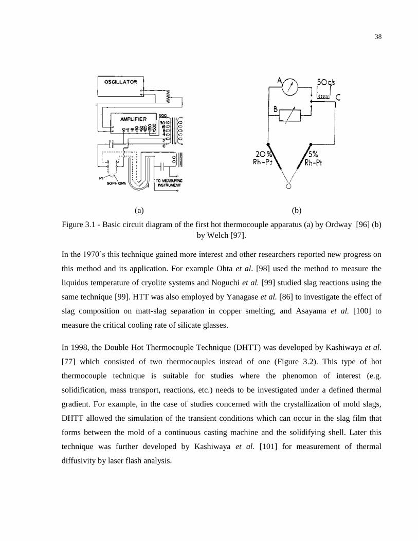
38

(a) (b)

Figure 3.1 - Basic circuit diagram of the first hot thermocouple apparatus (a) by Ordway [96] (b)

by Welch [97].

In the 1970’s this technique gained more interest and other researchers reported new progress on

this method and its application. For example Ohta et al. [98] used the method to measure the

liquidus temperature of cryolite systems and Noguchi et al. [99] studied slag reactions using the

same technique [99]. HTT was also employed by Yanagase et al. [86] to investigate the effect of

slag composition on matt-slag separation in copper smelting, and Asayama et al. [100] to

measure the critical cooling rate of silicate glasses.

In 1998, the Double Hot Thermocouple Technique (DHTT) was developed by Kashiwaya et al.

[77] which consisted of two thermocouples instead of one (Figure 3.2). This type of hot

thermocouple technique is suitable for studies where the phenomon of interest (e.g.

solidification, mass transport, reactions, etc.) needs to be investigated under a defined thermal

gradient. For example, in the case of studies concerned with the crystallization of mold slags,

DHTT allowed the simulation of the transient conditions which can occur in the slag film that

forms between the mold of a continuous casting machine and the solidifying shell. Later this

technique was further developed by Kashiwaya et al. [101] for measurement of thermal

diffusivity by laser flash analysis.

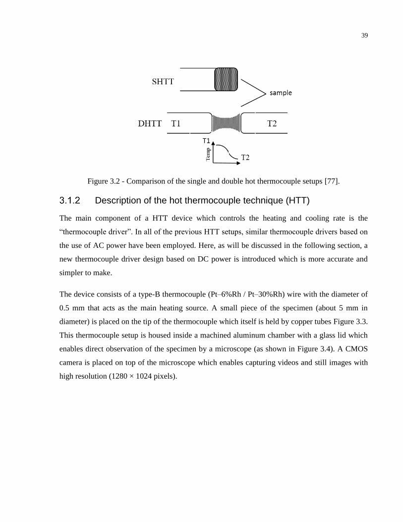
39

Figure 3.2 - Comparison of the single and double hot thermocouple setups [77].

Description of the hot thermocouple technique (HTT)

The main component of a HTT device which controls the heating and cooling rate is the

“thermocouple driver”. In all of the previous HTT setups, similar thermocouple drivers based on

the use of AC power have been employed. Here, as will be discussed in the following section, a

new thermocouple driver design based on DC power is introduced which is more accurate and

simpler to make.

The device consists of a type-B thermocouple (Pt–6%Rh / Pt–30%Rh) wire with the diameter of

0.5 mm that acts as the main heating source. A small piece of the specimen (about 5 mm in

diameter) is placed on the tip of the thermocouple which itself is held by copper tubes Figure 3.3.

This thermocouple setup is housed inside a machined aluminum chamber with a glass lid which

enables direct observation of the specimen by a microscope (as shown in Figure 3.4). A CMOS

camera is placed on top of the microscope which enables capturing videos and still images with

high resolution (1280 × 1024 pixels).

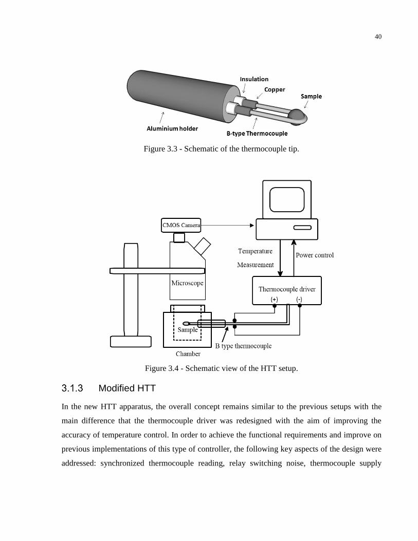
40

Figure 3.3 - Schematic of the thermocouple tip.

Figure 3.4 - Schematic view of the HTT setup.

Modified HTT

In the new HTT apparatus, the overall concept remains similar to the previous setups with the

main difference that the thermocouple driver was redesigned with the aim of improving the

accuracy of temperature control. In order to achieve the functional requirements and improve on

previous implementations of this type of controller, the following key aspects of the design were

addressed: synchronized thermocouple reading, relay switching noise, thermocouple supply

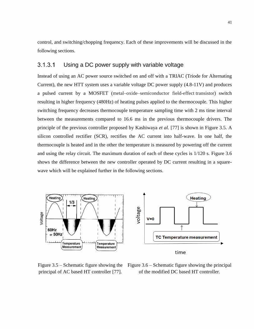
41

control, and switching/chopping frequency. Each of these improvements will be discussed in the

following sections.

Using a DC power supply with variable voltage

Instead of using an AC power source switched on and off with a TRIAC (Triode for Alternating

Current), the new HTT system uses a variable voltage DC power supply (4.8-11V) and produces

a pulsed current by a MOSFET (metal–oxide–semiconductor field-effect transistor) switch

resulting in higher frequency (480Hz) of heating pulses applied to the thermocouple. This higher

switching frequency decreases thermocouple temperature sampling time with 2 ms time interval

between the measurements compared to 16.6 ms in the previous thermocouple drivers. The

principle of the previous controller proposed by Kashiwaya et al. [77] is shown in Figure 3.5. A

silicon controlled rectifier (SCR), rectifies the AC current into half-wave. In one half, the

thermocouple is heated and in the other the temperature is measured by powering off the current

and using the relay circuit. The maximum duration of each of these cycles is 1/120 s. Figure 3.6

shows the difference between the new controller operated by DC current resulting in a square-

wave which will be explained further in the following sections.

Figure 3.5 – Schematic figure showing the

principal of AC based HT controller [77].

Figure 3.6 – Schematic figure showing the principal

of the modified DC based HT controller.

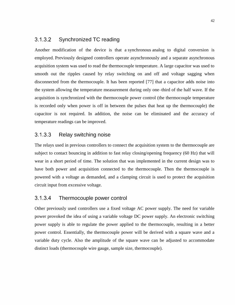
42

Synchronized TC reading

Another modification of the device is that a synchronous analog to digital conversion is

employed. Previously designed controllers operate asynchronously and a separate asynchronous

acquisition system was used to read the thermocouple temperature. A large capacitor was used to

smooth out the ripples caused by relay switching on and off and voltage sagging when

disconnected from the thermocouple. It has been reported [77] that a capacitor adds noise into

the system allowing the temperature measurement during only one–third of the half wave. If the

acquisition is synchronized with the thermocouple power control (the thermocouple temperature

is recorded only when power is off in between the pulses that heat up the thermocouple) the

capacitor is not required. In addition, the noise can be eliminated and the accuracy of

temperature readings can be improved.

Relay switching noise

The relays used in previous controllers to connect the acquisition system to the thermocouple are

subject to contact bouncing in addition to fast relay closing/opening frequency (60 Hz) that will

wear in a short period of time. The solution that was implemented in the current design was to

have both power and acquisition connected to the thermocouple. Then the thermocouple is

powered with a voltage as demanded, and a clamping circuit is used to protect the acquisition

circuit input from excessive voltage.

Thermocouple power control

Other previously used controllers use a fixed voltage AC power supply. The need for variable

power provoked the idea of using a variable voltage DC power supply. An electronic switching

power supply is able to regulate the power applied to the thermocouple, resulting in a better

power control. Essentially, the thermocouple power will be derived with a square wave and a

variable duty cycle. Also the amplitude of the square wave can be adjusted to accommodate

distinct loads (thermocouple wire gauge, sample size, thermocouple).

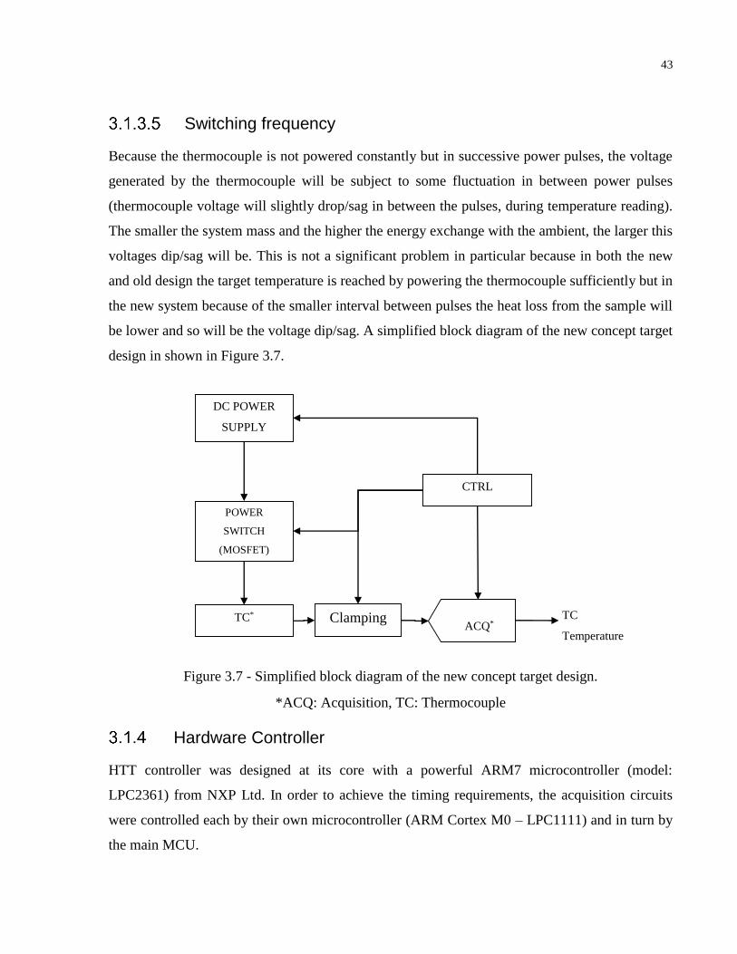
43

Switching frequency

Because the thermocouple is not powered constantly but in successive power pulses, the voltage

generated by the thermocouple will be subject to some fluctuation in between power pulses

(thermocouple voltage will slightly drop/sag in between the pulses, during temperature reading).

The smaller the system mass and the higher the energy exchange with the ambient, the larger this

voltages dip/sag will be. This is not a significant problem in particular because in both the new

and old design the target temperature is reached by powering the thermocouple sufficiently but in

the new system because of the smaller interval between pulses the heat loss from the sample will

be lower and so will be the voltage dip/sag. A simplified block diagram of the new concept target

design in shown in Figure 3.7.

Figure 3.7 - Simplified block diagram of the new concept target design.

*ACQ: Acquisition, TC: Thermocouple

Hardware Controller

HTT controller was designed at its core with a powerful ARM7 microcontroller (model:

LPC2361) from NXP Ltd. In order to achieve the timing requirements, the acquisition circuits

were controlled each by their own microcontroller (ARM Cortex M0 – LPC1111) and in turn by

the main MCU.

DC POWER

SUPPLY

POWER

SWITCH

(MOSFET)

TC*

CTRL

ACQ* TC

Temperature

Reading

Clamping

44

The hot thermocouple driver in this study was initially intended for use in SHTT mode but was

designed so that it is also suitable for tests that require a thermal gradient (i.e. used as a DHTT).

Therefore, two separate variable DC power supplies were used to allow applying an external

differential voltage between the two thermocouples. In order to connect the acquisition circuit

input directly to the thermocouple and still have the two channels separated for DHTT

applications, the two channels (power supplies and acquisition circuits) are completely isolated

from each other and from the main MCU. Therefore, the presence of the isolation block in the

diagram provides galvanic isolation between the two channels and main MCU. A complete block

diagram of the controller is shown in Figure 3.8.

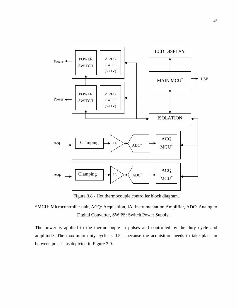
45

Figure 3.8 - Hot thermocouple controller block diagram.

*MCU: Microcontroller unit, ACQ: Acquisition, IA: Instrumentation Amplifier, ADC: Analog to

Digital Converter, SW PS: Switch Power Supply.

The power is applied to the thermocouple in pulses and controlled by the duty cycle and

amplitude. The maximum duty cycle is 0.5 s because the acquisition needs to take place in

between pulses, as depicted in Figure 3.9.

MAIN MCU*

LCD DISPLAY

ACQ

MCU*

ADC* Clamping

AC/DC

SW PS

(5-11V)

Power

CH1

IA

ACQ

MCU*

ADC* Clamping IA

AC/DC

SW PS

(5-11V)

POWER

SWITCH

ISOLATION

POWER

SWITCH Power

CH2

Acq.

CH1

Acq.

CH2

USB

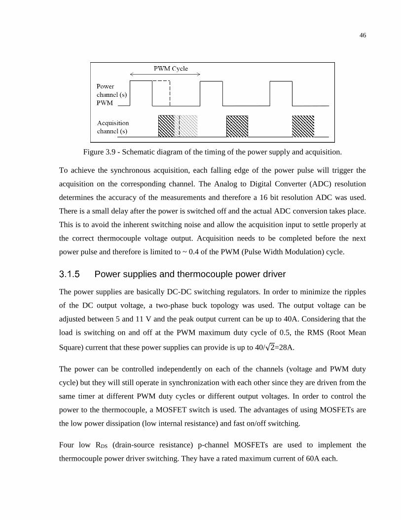
46

Figure 3.9 - Schematic diagram of the timing of the power supply and acquisition.

To achieve the synchronous acquisition, each falling edge of the power pulse will trigger the

acquisition on the corresponding channel. The Analog to Digital Converter (ADC) resolution

determines the accuracy of the measurements and therefore a 16 bit resolution ADC was used.

There is a small delay after the power is switched off and the actual ADC conversion takes place.

This is to avoid the inherent switching noise and allow the acquisition input to settle properly at

the correct thermocouple voltage output. Acquisition needs to be completed before the next

power pulse and therefore is limited to ~ 0.4 of the PWM (Pulse Width Modulation) cycle.

Power supplies and thermocouple power driver

The power supplies are basically DC-DC switching regulators. In order to minimize the ripples

of the DC output voltage, a two-phase buck topology was used. The output voltage can be

adjusted between 5 and 11 V and the peak output current can be up to 40A. Considering that the

load is switching on and off at the PWM maximum duty cycle of 0.5, the RMS (Root Mean

Square) current that these power supplies can provide is up to 40/√2=28A.

The power can be controlled independently on each of the channels (voltage and PWM duty

cycle) but they will still operate in synchronization with each other since they are driven from the

same timer at different PWM duty cycles or different output voltages. In order to control the

power to the thermocouple, a MOSFET switch is used. The advantages of using MOSFETs are

the low power dissipation (low internal resistance) and fast on/off switching.

Four low RDS (drain-source resistance) p-channel MOSFETs are used to implement the

thermocouple power driver switching. They have a rated maximum current of 60A each.

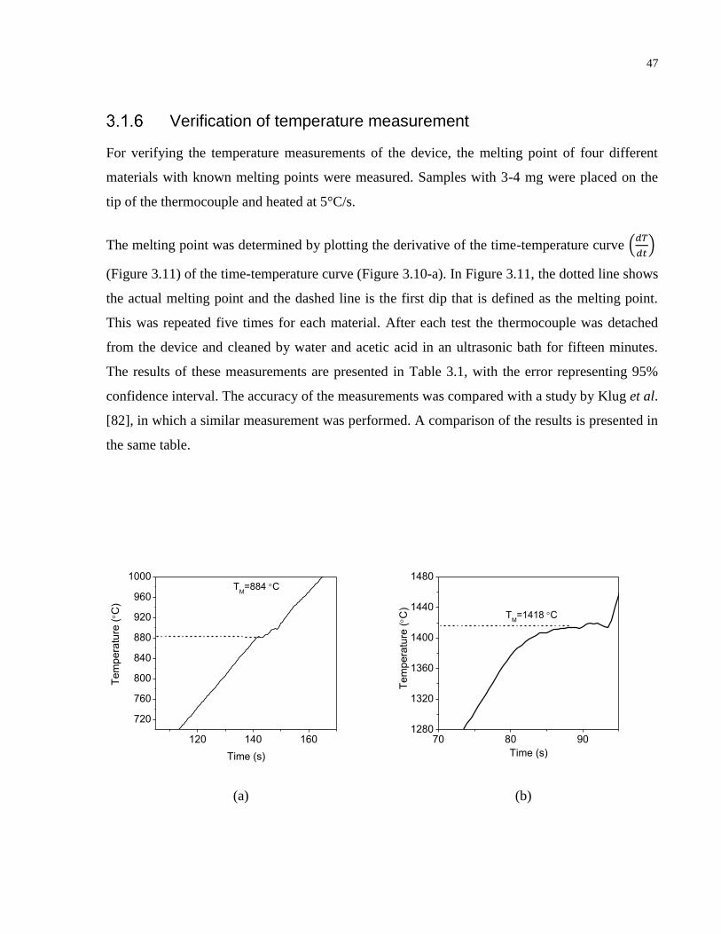
47

Verification of temperature measurement

For verifying the temperature measurements of the device, the melting point of four different

materials with known melting points were measured. Samples with 3-4 mg were placed on the

tip of the thermocouple and heated at 5°C/s.

The melting point was determined by plotting the derivative of the time-temperature curve (𝑑𝑇

𝑑𝑡)

(Figure 3.11) of the time-temperature curve (Figure 3.10-a). In Figure 3.11, the dotted line shows

the actual melting point and the dashed line is the first dip that is defined as the melting point.

This was repeated five times for each material. After each test the thermocouple was detached

from the device and cleaned by water and acetic acid in an ultrasonic bath for fifteen minutes.

The results of these measurements are presented in Table 3.1, with the error representing 95%

confidence interval. The accuracy of the measurements was compared with a study by Klug et al.

[82], in which a similar measurement was performed. A comparison of the results is presented in

the same table.

120 140 160

720

760

800

840

880

920

960

1000

Tem

pera

ture

(C

)

Time (s)

TM=884 C

70 80 901280

1320

1360

1400

1440

1480

TM=1418 C

Tem

pera

ture

(C

)

Time (s)

(a) (b)

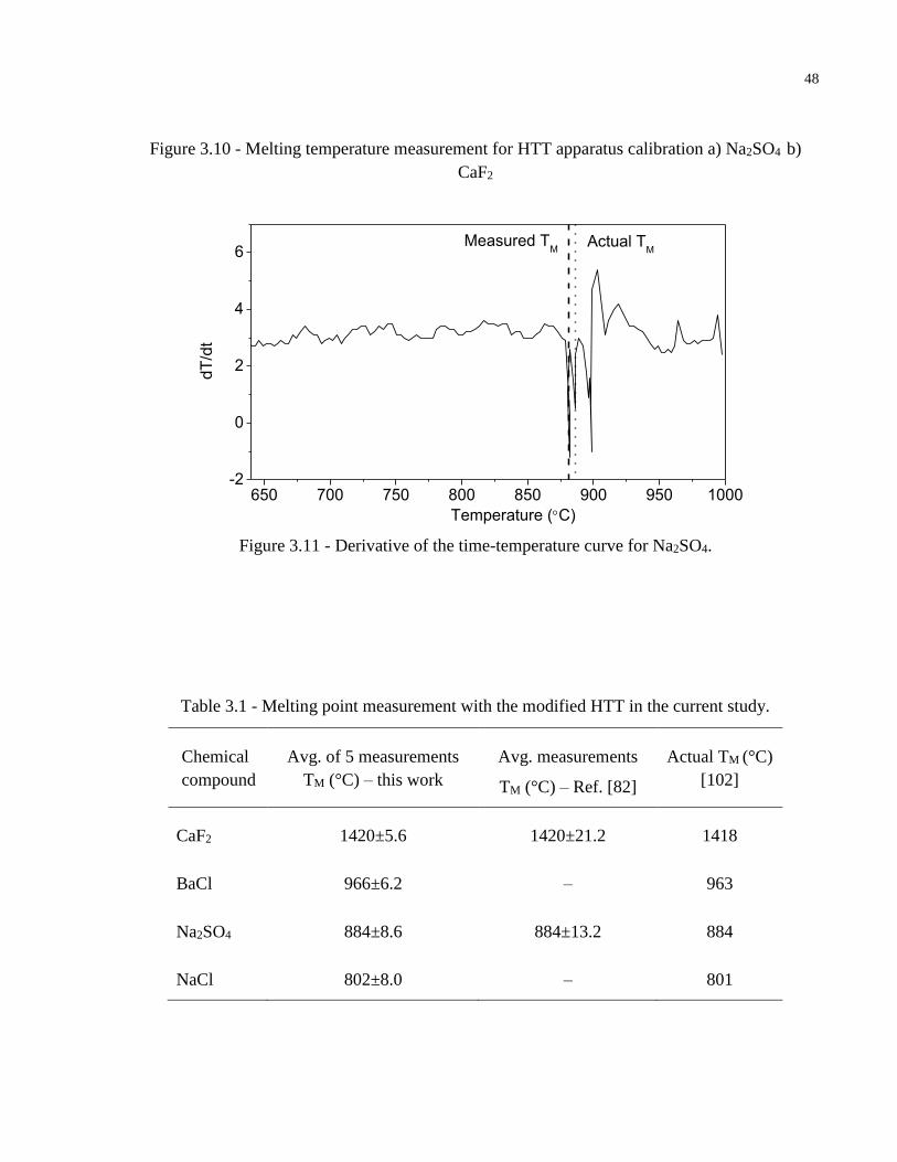
48

Figure 3.10 - Melting temperature measurement for HTT apparatus calibration a) Na2SO4 b)

CaF2

650 700 750 800 850 900 950 1000-2

0

2

4

6Measured T

MActual T

M

dT

/dt

Temperature (C)

Figure 3.11 - Derivative of the time-temperature curve for Na2SO4.

Table 3.1 - Melting point measurement with the modified HTT in the current study.

Chemical

compound

Avg. of 5 measurements

TM (°C) – this work

Avg. measurements

TM (°C) – Ref. [82]

Actual TM (°C)

[102]

CaF2 1420±5.6 1420±21.2 1418

BaCl 966±6.2 – 963

Na2SO4 884±8.6 884±13.2 884

NaCl 802±8.0 – 801

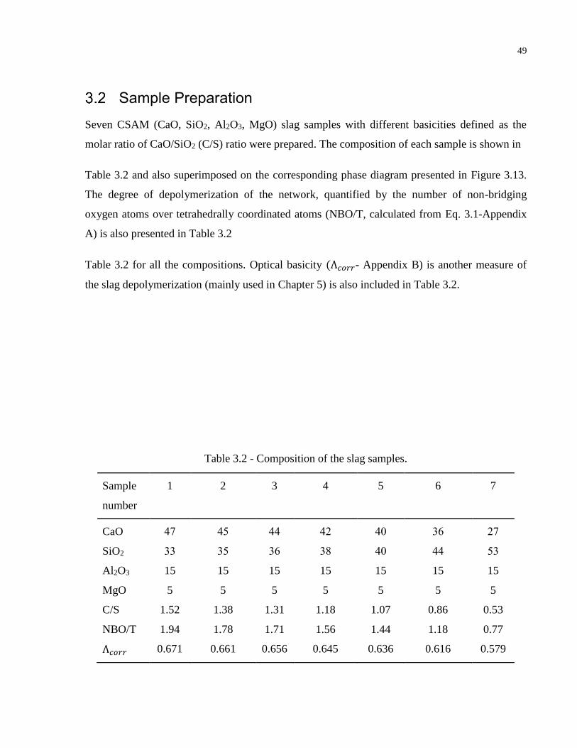
49

Sample Preparation

Seven CSAM (CaO, SiO2, Al2O3, MgO) slag samples with different basicities defined as the

molar ratio of CaO/SiO2 (C/S) ratio were prepared. The composition of each sample is shown in

Table 3.2 and also superimposed on the corresponding phase diagram presented in Figure 3.13.

The degree of depolymerization of the network, quantified by the number of non-bridging

oxygen atoms over tetrahedrally coordinated atoms (NBO/T, calculated from Eq. 3.1-Appendix

A) is also presented in Table 3.2

Table 3.2 for all the compositions. Optical basicity (Ʌ𝑐𝑜𝑟𝑟- Appendix B) is another measure of

the slag depolymerization (mainly used in Chapter 5) is also included in Table 3.2.

Table 3.2 - Composition of the slag samples.

Sample

number

1 2 3 4 5 6 7

CaO 47 45 44 42 40 36 27

SiO2 33 35 36 38 40 44 53

Al2O3 15 15 15 15 15 15 15

MgO 5 5 5 5 5 5 5

C/S 1.52 1.38 1.31 1.18 1.07 0.86 0.53

NBO/T 1.94 1.78 1.71 1.56 1.44 1.18 0.77

Ʌ𝑐𝑜𝑟𝑟 0.671 0.661 0.656 0.645 0.636 0.616 0.579

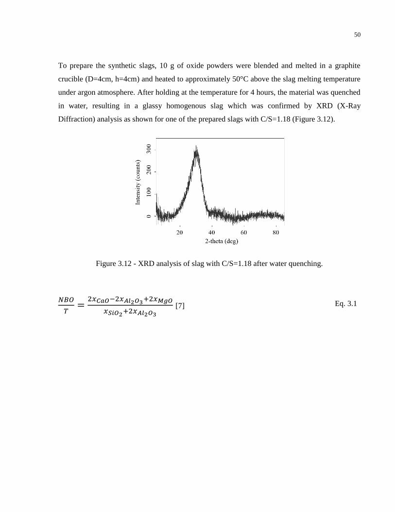
50

To prepare the synthetic slags, 10 g of oxide powders were blended and melted in a graphite

crucible (D=4cm, h=4cm) and heated to approximately 50°C above the slag melting temperature

under argon atmosphere. After holding at the temperature for 4 hours, the material was quenched

in water, resulting in a glassy homogenous slag which was confirmed by XRD (X-Ray

Diffraction) analysis as shown for one of the prepared slags with C/S=1.18 (Figure 3.12).

Figure 3.12 - XRD analysis of slag with C/S=1.18 after water quenching.

𝑁𝐵𝑂

𝑇=

2𝑥𝐶𝑎𝑂−2𝑥𝐴𝑙2𝑂3+2𝑥𝑀𝑔𝑂

𝑥𝑆𝑖𝑂2+2𝑥𝐴𝑙2𝑂3

[7] Eq. 3.1

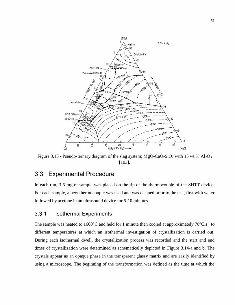
51

Figure 3.13 - Pseudo-ternary diagram of the slag system; MgO-CaO-SiO2 with 15 wt % Al2O3

[103].

Experimental Procedure

In each run, 3-5 mg of sample was placed on the tip of the thermocouple of the SHTT device.

For each sample, a new thermocouple was used and was cleaned prior to the test, first with water

followed by acetone in an ultrasound device for 5-10 minutes.

Isothermal Experiments

The sample was heated to 1600°C and held for 1 minute then cooled at approximately 70°C.s-1 to

different temperatures at which an isothermal investigation of crystallization is carried out.

During each isothermal dwell, the crystallization process was recorded and the start and end

times of crystallization were determined as schematically depicted in Figure 3.14-a and b. The

crystals appear as an opaque phase in the transparent glassy matrix and are easily identified by

using a microscope. The beginning of the transformation was defined as the time at which the

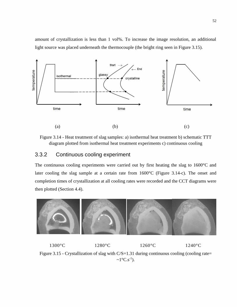
52

amount of crystallization is less than 1 vol%. To increase the image resolution, an additional

light source was placed underneath the thermocouple (the bright ring seen in Figure 3.15).

(a) (b) (c)

Figure 3.14 - Heat treatment of slag samples: a) isothermal heat treatment b) schematic TTT

diagram plotted from isothermal heat treatment experiments c) continuous cooling

Continuous cooling experiment

The continuous cooling experiments were carried out by first heating the slag to 1600°C and

later cooling the slag sample at a certain rate from 1600°C (Figure 3.14-c). The onset and

completion times of crystallization at all cooling rates were recorded and the CCT diagrams were

then plotted (Section 4.4).

1300°C 1280°C 1260°C 1240°C

Figure 3.15 - Crystallization of slag with C/S=1.31 during continuous cooling (cooling rate=

~1°C.s-1).

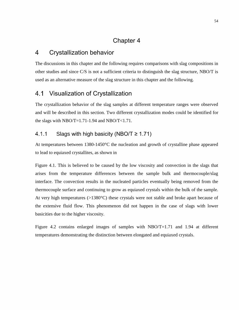
54

Chapter 4

Crystallization behavior

The discussions in this chapter and the following requires comparisons with slag compositions in

other studies and since C/S is not a sufficient criteria to distinguish the slag structure, NBO/T is

used as an alternative measure of the slag structure in this chapter and the following.

Visualization of Crystallization

The crystallization behavior of the slag samples at different temperature ranges were observed

and will be described in this section. Two different crystallization modes could be identified for

the slags with NBO/T=1.71-1.94 and NBO/T<1.71.

Slags with high basicity (NBO/T ≥ 1.71)

At temperatures between 1380-1450°C the nucleation and growth of crystalline phase appeared

to lead to equiaxed crystallites, as shown in

Figure 4.1. This is believed to be caused by the low viscosity and convection in the slags that

arises from the temperature differences between the sample bulk and thermocouple/slag

interface. The convection results in the nucleated particles eventually being removed from the

thermocouple surface and continuing to grow as equiaxed crystals within the bulk of the sample.

At very high temperatures (>1380°C) these crystals were not stable and broke apart because of

the extensive fluid flow. This phenomenon did not happen in the case of slags with lower

basicities due to the higher viscosity.

Figure 4.2 contains enlarged images of samples with NBO/T=1.71 and 1.94 at different

temperatures demonstrating the distinction between elongated and equiaxed crystals.

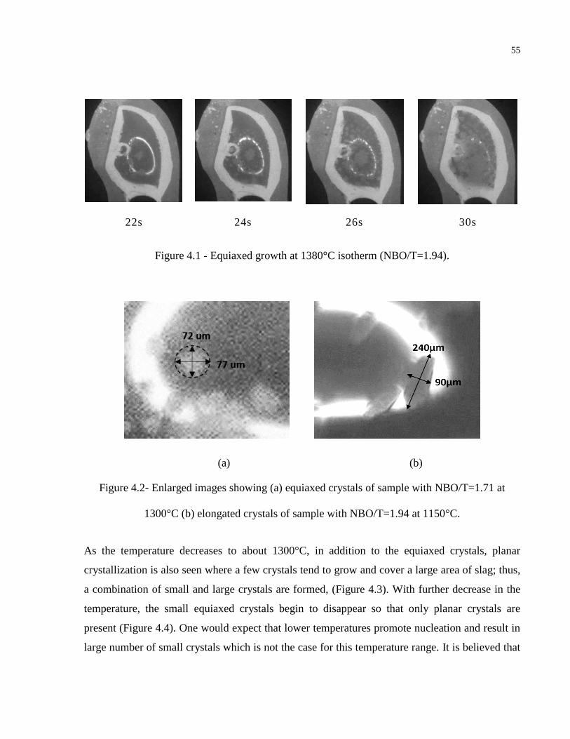
55

22s 24s 26s 30s

Figure 4.1 - Equiaxed growth at 1380°C isotherm (NBO/T=1.94).

(a) (b)

Figure 4.2- Enlarged images showing (a) equiaxed crystals of sample with NBO/T=1.71 at

1300°C (b) elongated crystals of sample with NBO/T=1.94 at 1150°C.

As the temperature decreases to about 1300°C, in addition to the equiaxed crystals, planar

crystallization is also seen where a few crystals tend to grow and cover a large area of slag; thus,

a combination of small and large crystals are formed, (Figure 4.3). With further decrease in the

temperature, the small equiaxed crystals begin to disappear so that only planar crystals are

present (Figure 4.4). One would expect that lower temperatures promote nucleation and result in

large number of small crystals which is not the case for this temperature range. It is believed that

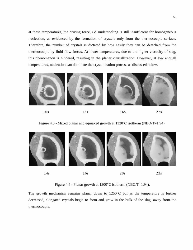
56

at these temperatures, the driving force, i.e. undercooling is still insufficient for homogeneous

nucleation, as evidenced by the formation of crystals only from the thermocouple surface.

Therefore, the number of crystals is dictated by how easily they can be detached from the

thermocouple by fluid flow forces. At lower temperatures, due to the higher viscosity of slag,

this phenomenon is hindered, resulting in the planar crystallization. However, at low enough

temperatures, nucleation can dominate the crystallization process as discussed below.

10s 12s 16s 27s

Figure 4.3 - Mixed planar and equiaxed growth at 1320ºC isotherm (NBO/T=1.94).

14s 16s 20s 23s

Figure 4.4 - Planar growth at 1300°C isotherm (NBO/T=1.94).

The growth mechanism remains planar down to 1250°C but as the temperature is further

decreased, elongated crystals begin to form and grow in the bulk of the slag, away from the

thermocouple.

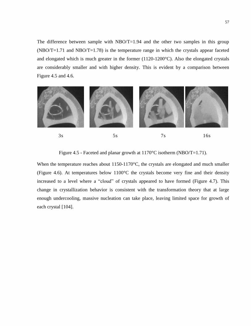
57

The difference between sample with NBO/T=1.94 and the other two samples in this group

(NBO/T=1.71 and NBO/T=1.78) is the temperature range in which the crystals appear faceted

and elongated which is much greater in the former (1120-1200°C). Also the elongated crystals

are considerably smaller and with higher density. This is evident by a comparison between

Figure 4.5 and 4.6.

o o o o

3s 5s 7s 16s

Figure 4.5 - Faceted and planar growth at 1170°C isotherm (NBO/T=1.71).

When the temperature reaches about 1150-1170°C, the crystals are elongated and much smaller

(Figure 4.6). At temperatures below 1100°C the crystals become very fine and their density

increased to a level where a “cloud” of crystals appeared to have formed (Figure 4.7). This

change in crystallization behavior is consistent with the transformation theory that at large

enough undercooling, massive nucleation can take place, leaving limited space for growth of

each crystal [104].

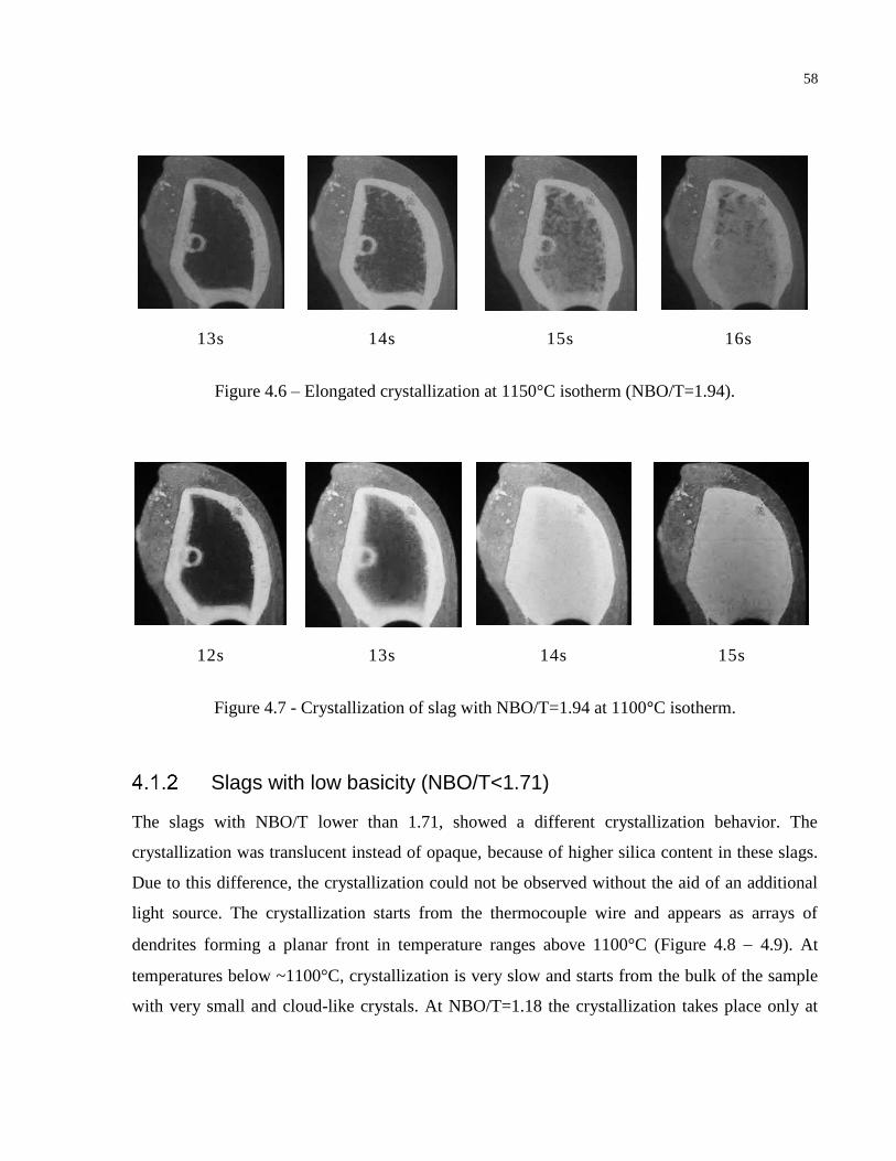
58

13s 14s 15s 16s

Figure 4.6 – Elongated crystallization at 1150°C isotherm (NBO/T=1.94).

12s 13s 14s 15s

Figure 4.7 - Crystallization of slag with NBO/T=1.94 at 1100°C isotherm.

Slags with low basicity (NBO/T<1.71)

The slags with NBO/T lower than 1.71, showed a different crystallization behavior. The

crystallization was translucent instead of opaque, because of higher silica content in these slags.

Due to this difference, the crystallization could not be observed without the aid of an additional

light source. The crystallization starts from the thermocouple wire and appears as arrays of

dendrites forming a planar front in temperature ranges above 1100°C (Figure 4.8 4.9). At

temperatures below ~1100°C, crystallization is very slow and starts from the bulk of the sample

with very small and cloud-like crystals. At NBO/T=1.18 the crystallization takes place only at

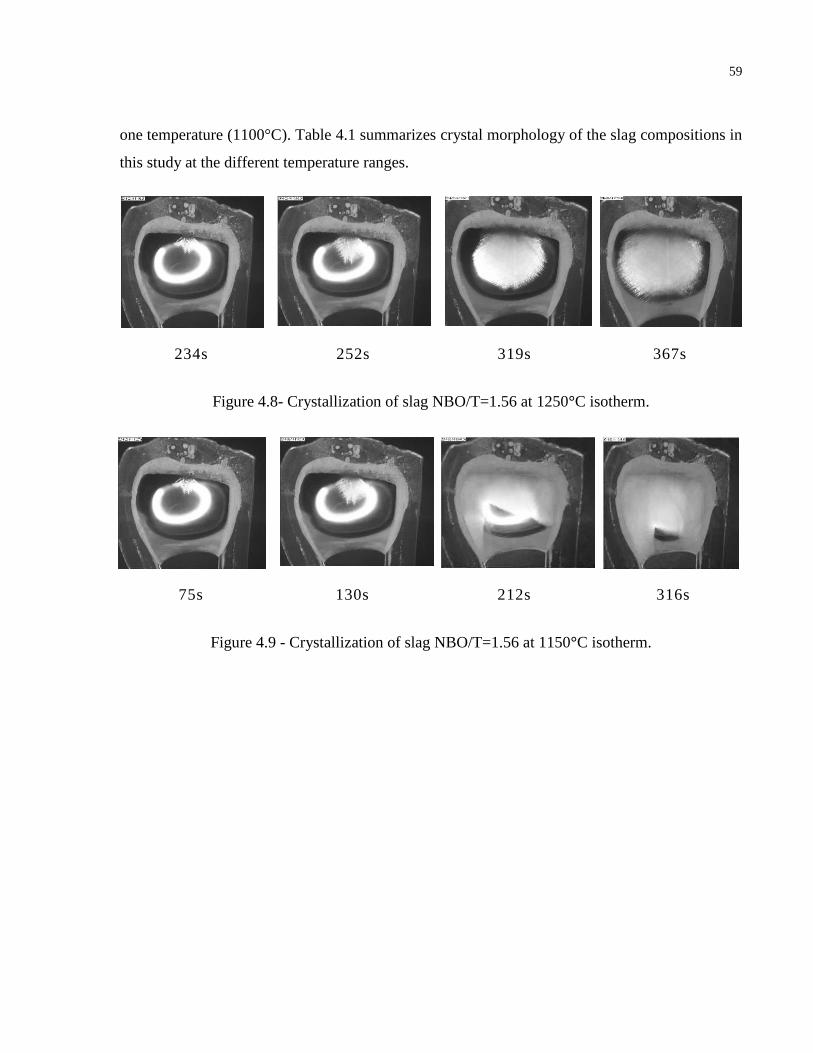
59

one temperature (1100°C). Table 4.1 summarizes crystal morphology of the slag compositions in

this study at the different temperature ranges.

234s 252s 319s 367s

Figure 4.8- Crystallization of slag NBO/T=1.56 at 1250°C isotherm.

75s 130s 212s 316s

Figure 4.9 - Crystallization of slag NBO/T=1.56 at 1150°C isotherm.

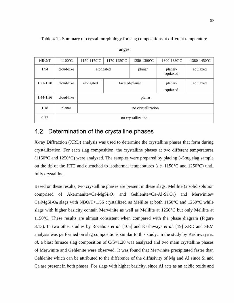
60

Table 4.1 - Summary of crystal morphology for slag compositions at different temperature

ranges.

NBO/T 1100°C 1150-1170°C 1170-1250°C 1250-1300°C 1300-1380°C 1380-1450°C

1.94 cloud-like elongated planar planar-

equiaxed

equiaxed

1.71-1.78 cloud-like elongated faceted-planar planar-

equiaxed

equiaxed

1.44-1.56 cloud-like planar

1.18 planar no crystallization

0.77 no crystallization

Determination of the crystalline phases

X-ray Diffraction (XRD) analysis was used to determine the crystalline phases that form during

crystallization. For each slag composition, the crystalline phases at two different temperatures

(1150°C and 1250°C) were analyzed. The samples were prepared by placing 3-5mg slag sample

on the tip of the HTT and quenched to isothermal temperatures (i.e. 1150°C and 1250°C) until

fully crystalline.

Based on these results, two crystalline phases are present in these slags: Melilite (a solid solution

comprised of Akermanite=Ca2MgSi2O7 and Gehlenite=Ca2Al2Si2O7) and Merwinite=

Ca3MgSi2O8 slags with NBO/T<1.56 crystallized as Melilite at both 1150°C and 1250°C while

slags with higher basicity contain Merwinite as well as Melilite at 1250°C but only Melilite at

1150°C. These results are almost consistent when compared with the phase diagram (Figure

3.13). In two other studies by Rocabois et al. [105] and Kashiwaya et al. [19] XRD and SEM

analysis was performed on slag compositions similar to this study. In the study by Kashiwaya et

al. a blast furnace slag composition of C/S=1.28 was analyzed and two main crystalline phases

of Merwinite and Gehlenite were observed. It was found that Merwinite precipitated faster than

Gehlenite which can be attributed to the difference of the diffusivity of Mg and Al since Si and

Ca are present in both phases. For slags with higher basicity, since Al acts as an acidic oxide and

61

forms AlO4-5 tetrahedron in the silicate structure, it is more difficult for it to migrate compared to

Mg. In addition, since Merwinite has lower Gibbs free energy of formation, it has higher driving

force to form.

Time-Temperature-Transformation (TTT) diagram

The TTT diagrams of different slag compositions are shown in Figure 4.10. The sample with a

NBO/T=0.77 did not crystallize at any temperature. Also, the sample with NBO/T=1.18 only

crystallized at a single temperature (shown as a point in Figure 4.10 - a). The start curve of TTT

diagrams of six slag samples are shown in Figure 4.11.

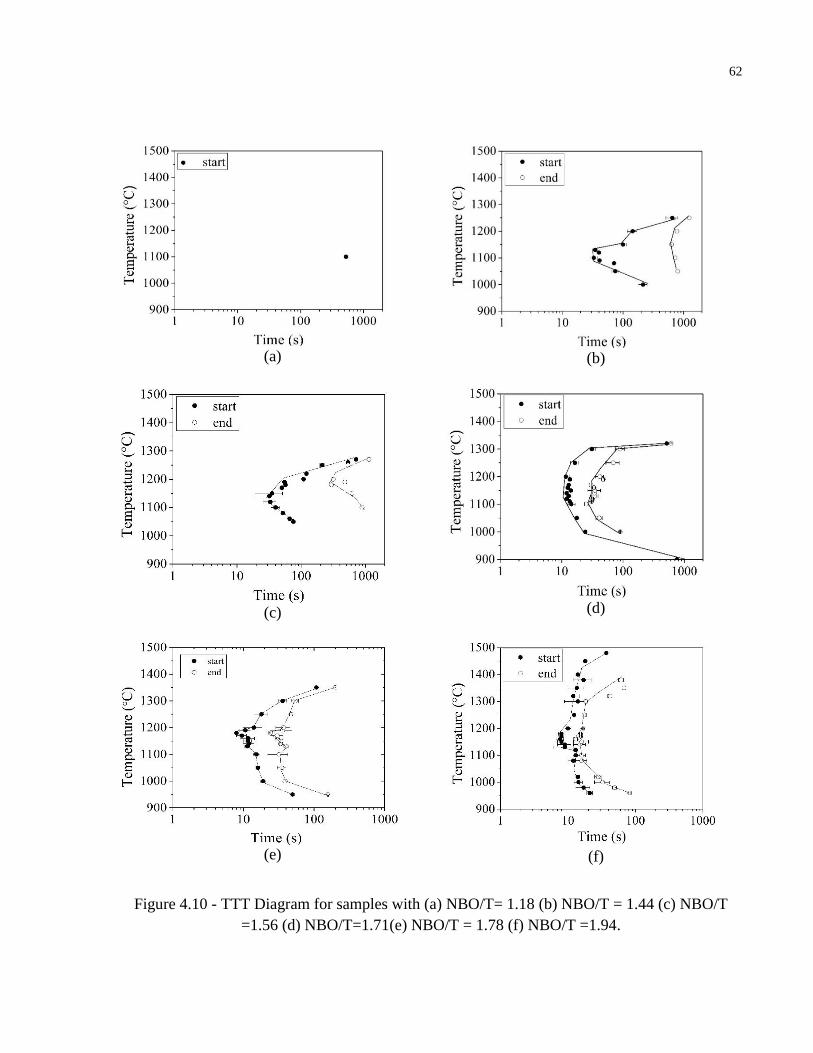
62

(a)

(b)

(c)

(d)

(e)

(f)

Figure 4.10 - TTT Diagram for samples with (a) NBO/T= 1.18 (b) NBO/T = 1.44 (c) NBO/T

=1.56 (d) NBO/T=1.71(e) NBO/T = 1.78 (f) NBO/T =1.94.

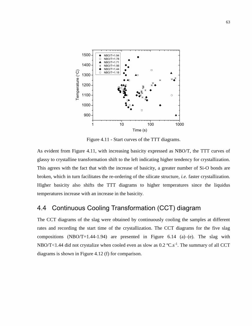
63

1 10 100 1000

900

1000

1100

1200

1300

1400

1500 NBO/T=1.94

NBO/T=1.78

NBO/T=1.71

NBO/T=1.56

NBO/T=1.44

NBO/T=1.18

Te

mp

era

ture

(C

)

Time (s)

Figure 4.11 - Start curves of the TTT diagrams.

As evident from Figure 4.11, with increasing basicity expressed as NBO/T, the TTT curves of

glassy to crystalline transformation shift to the left indicating higher tendency for crystallization.

This agrees with the fact that with the increase of basicity, a greater number of Si-O bonds are

broken, which in turn facilitates the re-ordering of the silicate structure, i.e. faster crystallization.

Higher basicity also shifts the TTT diagrams to higher temperatures since the liquidus

temperatures increase with an increase in the basicity.

Continuous Cooling Transformation (CCT) diagram

The CCT diagrams of the slag were obtained by continuously cooling the samples at different

rates and recording the start time of the crystallization. The CCT diagrams for the five slag

compositions (NBO/T=1.44-1.94) are presented in Figure 6.14 (a)–(e). The slag with

NBO/T<1.44 did not crystalize when cooled even as slow as 0.2 ºC.s-1. The summary of all CCT

diagrams is shown in Figure 4.12 (f) for comparison.

64

(a)

(b)

(c)

(d)

(e)

(f)

Figure 4.12 - CCT Diagram for slag samples with (a) NBO/T = 1.44 (b) NBO/T = 1.56 (c)

NBO/T = 1.71(d) NBO/T = 1.78 (e) NBO/T = 1.94 (f) Comparison of all CCT diagrams.

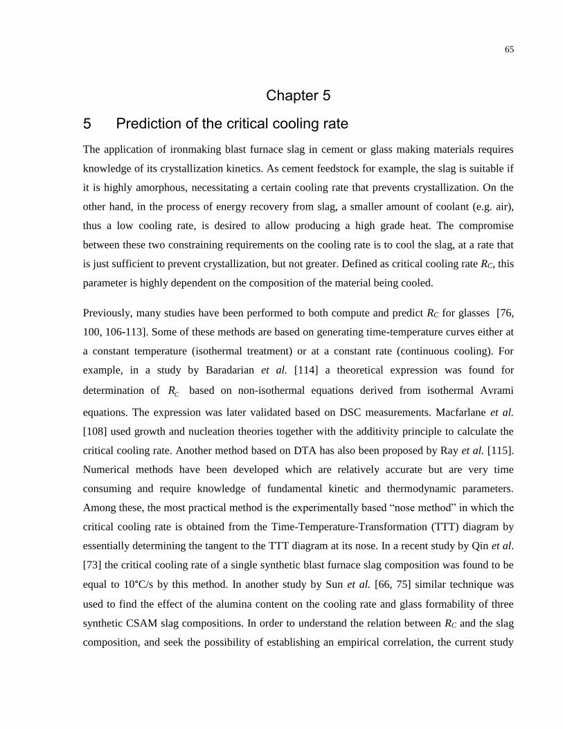
65

Chapter 5

Prediction of the critical cooling rate

The application of ironmaking blast furnace slag in cement or glass making materials requires

knowledge of its crystallization kinetics. As cement feedstock for example, the slag is suitable if

it is highly amorphous, necessitating a certain cooling rate that prevents crystallization. On the

other hand, in the process of energy recovery from slag, a smaller amount of coolant (e.g. air),

thus a low cooling rate, is desired to allow producing a high grade heat. The compromise

between these two constraining requirements on the cooling rate is to cool the slag, at a rate that

is just sufficient to prevent crystallization, but not greater. Defined as critical cooling rate RC, this

parameter is highly dependent on the composition of the material being cooled.

Previously, many studies have been performed to both compute and predict RC for glasses [76,

100, 106-113]. Some of these methods are based on generating time-temperature curves either at

a constant temperature (isothermal treatment) or at a constant rate (continuous cooling). For

example, in a study by Baradarian et al. [114] a theoretical expression was found for

determination of based on non-isothermal equations derived from isothermal Avrami

equations. The expression was later validated based on DSC measurements. Macfarlane et al.

[108] used growth and nucleation theories together with the additivity principle to calculate the

critical cooling rate. Another method based on DTA has also been proposed by Ray et al. [115].

Numerical methods have been developed which are relatively accurate but are very time

consuming and require knowledge of fundamental kinetic and thermodynamic parameters.

Among these, the most practical method is the experimentally based “nose method” in which the

critical cooling rate is obtained from the Time-Temperature-Transformation (TTT) diagram by

essentially determining the tangent to the TTT diagram at its nose. In a recent study by Qin et al.

[73] the critical cooling rate of a single synthetic blast furnace slag composition was found to be

equal to 10°C/s by this method. In another study by Sun et al. [66, 75] similar technique was

used to find the effect of the alumina content on the cooling rate and glass formability of three

synthetic CSAM slag compositions. In order to understand the relation between RC and the slag

composition, and seek the possibility of establishing an empirical correlation, the current study

CR

66

was conducted. Seven CaO-SiO2-Al2O3-MgO (CSAM) slags were prepared and their

crystallization behaviors were observed visually, and quantified by determining their TTT/CCT

(Continuous-Cooling-Transformation) diagrams, as described in the previous chapter. In this

chapter, those results together with data from 5 other studies, encompassing 44 slag

compositions were evaluated to investigate a possible relationship between slag composition and

RC. Further, the data were fitted to a model by Uhlmann and his co–workers [106, 116] to

establish a semi–empirical expression for estimating from the slag liquidus temperature and

viscosity.

Critical Cooling Rate

The critical cooling rate is the minimum cooling rate that results in a completely glassy slag (i.e.

no crystalline content) and can be found from Eq. 5.1.

𝑅𝐶(𝑇𝑇𝑇) =𝑇𝐿– 𝑇𝑛𝑜𝑠𝑒

𝑡𝑛𝑜𝑠𝑒

Eq. 5.1

where 𝑇𝐿 is the liquidus temperature, and tnose are the temperature and time corresponding

to the nose of the TTT or CCT diagrams, respectively. The nose of the diagram represents a

temperature at which the kinetics of transformation is the fastest, as a result of opposite

dependence of nucleation and growth to undercooling [117]. A tangent to the nose, originated

from the liquidus temperature ( ) yields RC. From the TTT diagrams of the above slags, Tnose

and tnose were obtained. Also, the liquidus temperature of each slag was determined using

FactSage™ thermodynamic package [118] (Table 5.1) which was also verified experimentally

by HTT. The results yielded the critical cooling rates of the slags, plotted against NBO/T in

Figure 5.1.

CR

noseT

LT

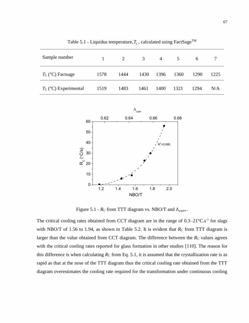
67

Table 5.1 - Liquidus temperature, , calculated using FactSageTM

Sample number 1 2 3 4 5 6 7

TL (°C) Factsage 1578 1444 1430 1396 1360 1290 1225

TL (°C) Experimental 1519 1483 1461 1400 1321 1294 N/A

1.2 1.4 1.6 1.8 2.00

10

20

30

40

50

60

corr

RC (C

/s)

NBO/T

0.62 0.64 0.66 0.68

R2=0.995

Figure 5.1 - RC from TTT diagram vs. NBO/T and Λ𝑐𝑜𝑟𝑟.

The critical cooling rates obtained from CCT diagram are in the range of 0.3–21°C.s-1 for slags

with NBO/T of 1.56 to 1.94, as shown in Table 5.2. It is evident that RC from TTT diagram is

larger than the value obtained from CCT diagram. The difference between the RC values agrees

with the critical cooling rates reported for glass formation in other studies [110]. The reason for

this difference is when calculating RC from Eq. 5.1, it is assumed that the crystallization rate is as

rapid as that at the nose of the TTT diagram thus the critical cooling rate obtained from the TTT

diagram overestimates the cooling rate required for the transformation under continuous cooling

LT

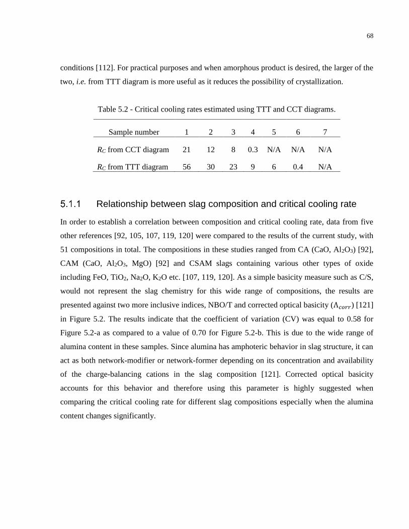
68

conditions [112]. For practical purposes and when amorphous product is desired, the larger of the

two, i.e. from TTT diagram is more useful as it reduces the possibility of crystallization.

Table 5.2 - Critical cooling rates estimated using TTT and CCT diagrams.

Sample number 1 2 3 4 5 6 7

RC from CCT diagram 21 12 8 0.3 N/A N/A N/A

RC from TTT diagram 56 30 23 9 6 0.4 N/A

Relationship between slag composition and critical cooling rate

In order to establish a correlation between composition and critical cooling rate, data from five

other references [92, 105, 107, 119, 120] were compared to the results of the current study, with

51 compositions in total. The compositions in these studies ranged from CA (CaO, Al2O3) [92],

CAM (CaO, Al2O3, MgO) [92] and CSAM slags containing various other types of oxide

including FeO, TiO2, Na2O, K2O etc. [107, 119, 120]. As a simple basicity measure such as C/S,

would not represent the slag chemistry for this wide range of compositions, the results are

presented against two more inclusive indices, NBO/T and corrected optical basicity (Λ𝑐𝑜𝑟𝑟) [121]

in Figure 5.2. The results indicate that the coefficient of variation (CV) was equal to 0.58 for

Figure 5.2-a as compared to a value of 0.70 for Figure 5.2-b. This is due to the wide range of

alumina content in these samples. Since alumina has amphoteric behavior in slag structure, it can

act as both network-modifier or network-former depending on its concentration and availability

of the charge-balancing cations in the slag composition [121]. Corrected optical basicity

accounts for this behavior and therefore using this parameter is highly suggested when

comparing the critical cooling rate for different slag compositions especially when the alumina

content changes significantly.

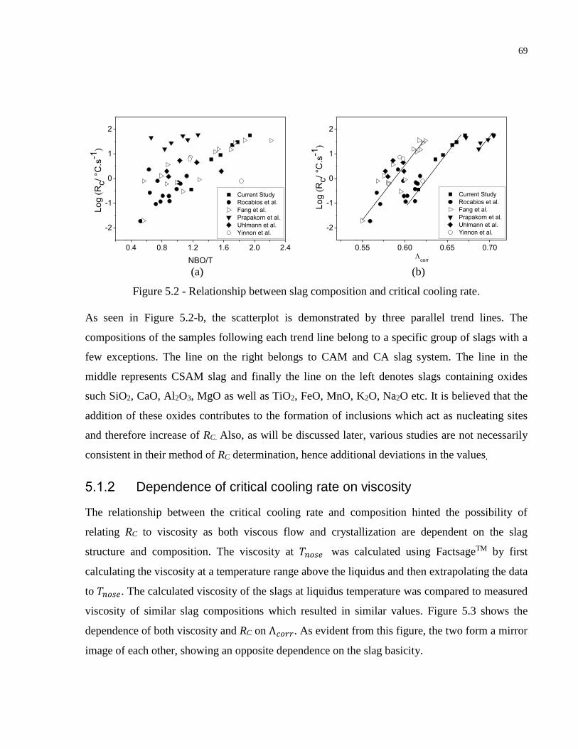
69

0.4 0.8 1.2 1.6 2.0 2.4

-2

-1

0

1

2

Current Study

Rocabios et al.

Fang et al.

Prapakorn et al.

Uhlmann et al.

Yinnon et al.

Lo

g (

Rc/

°C.s

-1)

NBO/T

(a)

0.55 0.60 0.65 0.70

-2

-1

0

1

2

Lo

g (

Rc/

°C.s

-1)

Current Study

Rocabios et al.

Fang et al.

Prapakorn et al.

Uhlmann et al.

Yinnon et al.

corr

(b)

Figure 5.2 - Relationship between slag composition and critical cooling rate.

As seen in Figure 5.2-b, the scatterplot is demonstrated by three parallel trend lines. The

compositions of the samples following each trend line belong to a specific group of slags with a

few exceptions. The line on the right belongs to CAM and CA slag system. The line in the

middle represents CSAM slag and finally the line on the left denotes slags containing oxides

such SiO2, CaO, Al2O3, MgO as well as TiO2, FeO, MnO, K2O, Na2O etc. It is believed that the

addition of these oxides contributes to the formation of inclusions which act as nucleating sites

and therefore increase of RC. Also, as will be discussed later, various studies are not necessarily

consistent in their method of RC determination, hence additional deviations in the values,

Dependence of critical cooling rate on viscosity

The relationship between the critical cooling rate and composition hinted the possibility of

relating RC to viscosity as both viscous flow and crystallization are dependent on the slag

structure and composition. The viscosity at 𝑇𝑛𝑜𝑠𝑒 was calculated using FactsageTM by first

calculating the viscosity at a temperature range above the liquidus and then extrapolating the data

to 𝑇𝑛𝑜𝑠𝑒. The calculated viscosity of the slags at liquidus temperature was compared to measured

viscosity of similar slag compositions which resulted in similar values. Figure 5.3 shows the

dependence of both viscosity and RC on Λ𝑐𝑜𝑟𝑟. As evident from this figure, the two form a mirror

image of each other, showing an opposite dependence on the slag basicity.

70

Figure 5.3 - RC and 𝜂𝑛𝑜𝑠𝑒 (Pa. s) vs. Λ𝑐𝑜𝑟𝑟.

A similar relation between viscosity at 𝑇𝐿 and RC could be seen (Figure 5.4), which is not

surprising, noting that the ratio of 𝑇𝑛𝑜𝑠𝑒

𝑇𝐿 is constant as explained below. In this figure, NBO/T is

again compared with optical basicity and it is shown that the correlation is stronger when using

Λ𝑐𝑜𝑟𝑟 (evident from CV value of 0.69 in Figure 5.4-a compared to 0.88 in Figure 5.4-b).

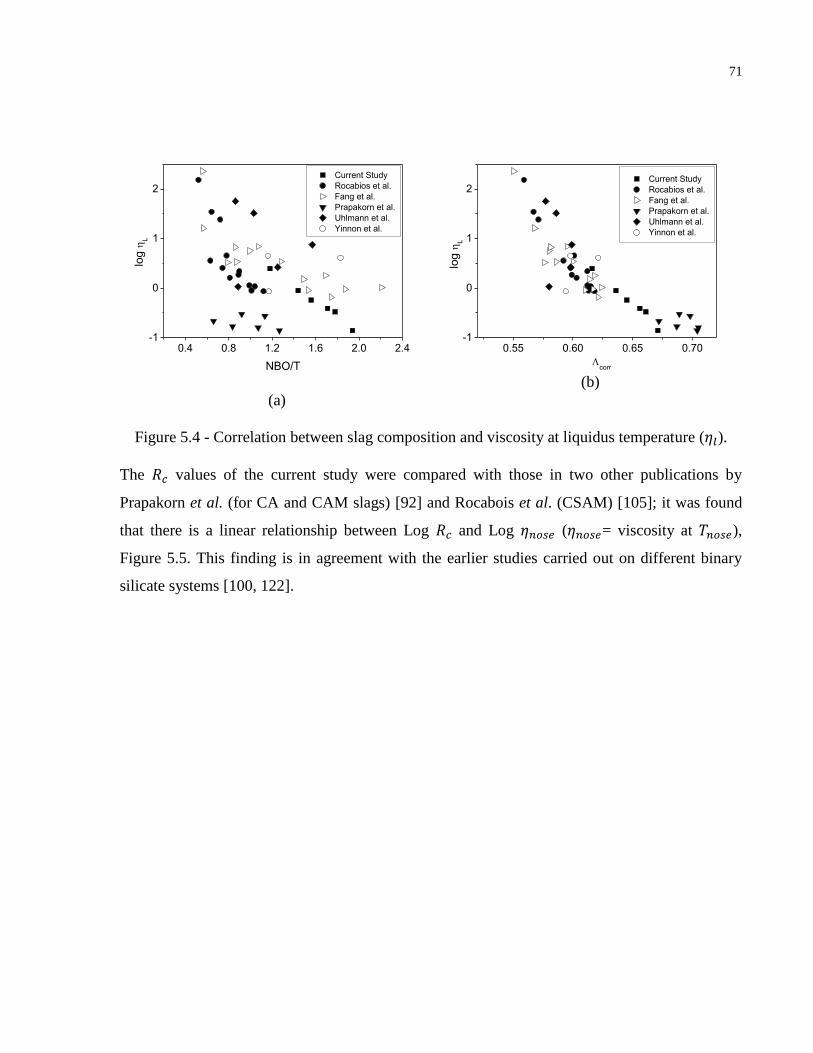
71

0.4 0.8 1.2 1.6 2.0 2.4-1

0

1

2

log

L

Current Study

Rocabios et al.

Fang et al.

Prapakorn et al.

Uhlmann et al.

Yinnon et al.

NBO/T

(a)

0.55 0.60 0.65 0.70-1

0

1

2

log

L

Current Study

Rocabios et al.

Fang et al.

Prapakorn et al.

Uhlmann et al.

Yinnon et al.

corr

(b)

Figure 5.4 - Correlation between slag composition and viscosity at liquidus temperature (𝜂𝑙).

The 𝑅𝑐 values of the current study were compared with those in two other publications by

Prapakorn et al. (for CA and CAM slags) [92] and Rocabois et al. (CSAM) [105]; it was found

that there is a linear relationship between Log 𝑅𝑐 and Log 𝜂𝑛𝑜𝑠𝑒 (𝜂𝑛𝑜𝑠𝑒= viscosity at 𝑇𝑛𝑜𝑠𝑒),

Figure 5.5. This finding is in agreement with the earlier studies carried out on different binary

silicate systems [100, 122].

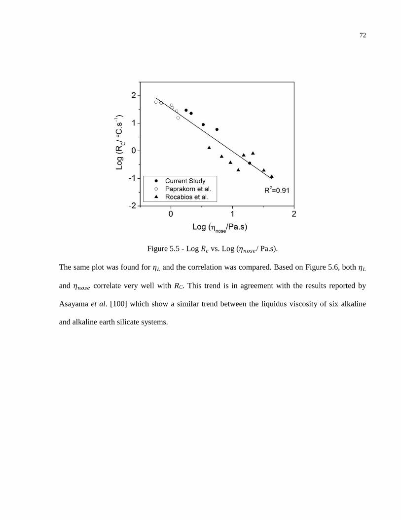
72

Figure 5.5 - Log 𝑅𝑐 vs. Log (𝜂𝑛𝑜𝑠𝑒/ Pa.s).

The same plot was found for 𝜂𝐿 and the correlation was compared. Based on Figure 5.6, both 𝜂𝐿

and 𝜂𝑛𝑜𝑠𝑒 correlate very well with RC. This trend is in agreement with the results reported by

Asayama et al. [100] which show a similar trend between the liquidus viscosity of six alkaline

and alkaline earth silicate systems.

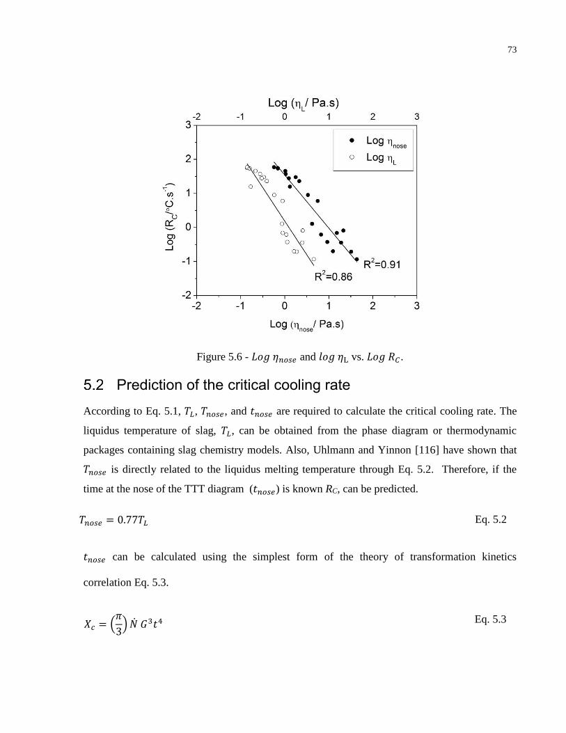
73

Figure 5.6 - 𝐿𝑜𝑔 𝜂𝑛𝑜𝑠𝑒 and 𝑙𝑜𝑔 𝜂L vs. 𝐿𝑜𝑔 𝑅𝐶 .

Prediction of the critical cooling rate

According to Eq. 5.1, 𝑇𝐿, 𝑇𝑛𝑜𝑠𝑒, and 𝑡𝑛𝑜𝑠𝑒 are required to calculate the critical cooling rate. The

liquidus temperature of slag, 𝑇𝐿, can be obtained from the phase diagram or thermodynamic

packages containing slag chemistry models. Also, Uhlmann and Yinnon [116] have shown that

𝑇𝑛𝑜𝑠𝑒 is directly related to the liquidus melting temperature through Eq. 5.2. Therefore, if the

time at the nose of the TTT diagram (𝑡𝑛𝑜𝑠𝑒) is known RC, can be predicted.

𝑇𝑛𝑜𝑠𝑒 = 0.77𝑇𝐿 Eq. 5.2

𝑡𝑛𝑜𝑠𝑒 can be calculated using the simplest form of the theory of transformation kinetics

correlation Eq. 5.3.

𝑋𝑐 = (𝜋

3) �� 𝐺3𝑡4 Eq. 5.3

74

In this equation, �� is the nucleation rate, 𝐺 is the growth rate, 𝑡 is transformation time and 𝑋𝑐 is

the minimum detectable transformed volume fraction, conventionally taken as 0.01.

𝑅𝑐 =(𝑇𝐿 − 𝑇𝑛𝑜𝑠𝑒)[

𝜋3 × �� × 𝐺3]1/4

𝑋𝑐1/4

Eq. 5.4

𝐺 and �� can be calculated using Eq. 5.5 and Eq. 5.6 [106].

�� = 𝐾′

𝜂𝑒𝑥𝑝 (

0.0205𝐵

𝛥𝑇𝑟2𝑇𝑟

3 ) Eq. 5.5

𝐺 = 𝐾′′𝑇𝐿

𝜂[1 − 𝑒𝑥𝑝(

−𝛥𝐻𝑀𝛥𝑇𝑟

𝑅𝑇𝑛𝑜𝑠𝑒)]

Eq. 5.6

where Δ𝑇𝑟 =Δ𝑇𝑛𝑜𝑠𝑒

𝑇𝐿 and 𝑇𝑟 =

𝑇𝑛𝑜𝑠𝑒

𝑇𝐿 and 𝑅 is gas constant.

The predictive expression for RC, Eq. 5.7, is obtained by substituting Eq. 5.5 and Eq. 5.6 into Eq.

5.4. This equation shows that 𝑅𝑐 can be calculated by only having three parameters (i.e. 𝜂𝑛𝑜𝑠𝑒,

𝑇𝑀 and ∆𝐻𝑀 = heat of fusion).

𝑅𝑐 =𝐴 𝑇𝐿

2

𝜂𝑛𝑜𝑠𝑒exp(−0.212𝐵) [1 − exp(

0.3 Δ𝐻𝑀

𝑅𝑇𝐿)]3/4

Eq. 5.7

In Eq. 5.7, 𝐵 is the nucleation barrier and can be found by plotting 𝑅𝑐 against λ=𝐴 𝑇𝐿

2

𝜂𝑛𝑜𝑠𝑒[1 −

exp(0.3 Δ𝐻𝑀

𝑅𝑇𝐿)]3/4for a set of measurements, with the slope of the line representing

𝑒𝑥𝑝 (−0.212𝐵) . In order to estimate the value of B, the required parameters (𝑇𝐿 , 𝜂𝑛𝑜𝑠𝑒, and

∆𝐻𝑀) were obtained by thermodynamic calculations for the slag compositions of the current

study. The ratios of 𝑇𝑛𝑜𝑠𝑒 𝑇𝐿⁄ for the present work and earlier reports [92, 105] are shown in

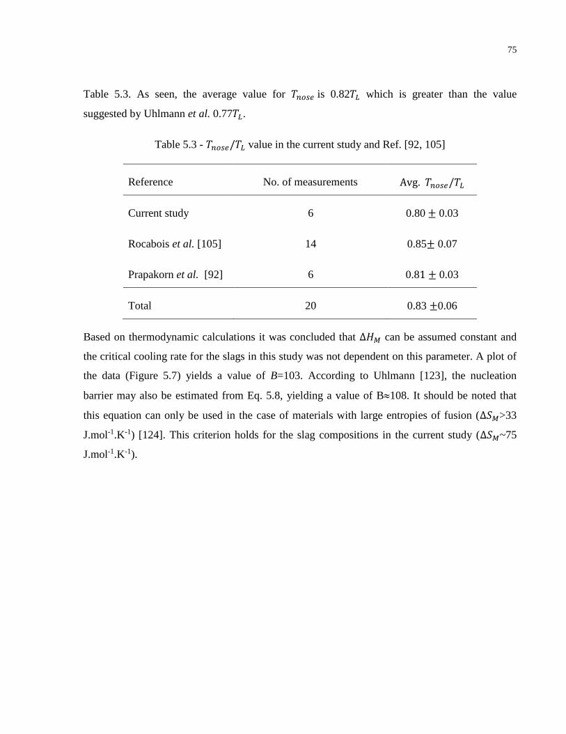
75

Table 5.3. As seen, the average value for 𝑇𝑛𝑜𝑠𝑒 is 0.82𝑇𝐿 which is greater than the value

suggested by Uhlmann et al. 0.77𝑇𝐿.

Table 5.3 - 𝑇𝑛𝑜𝑠𝑒/𝑇𝐿 value in the current study and Ref. [92, 105]

Reference No. of measurements Avg. 𝑇𝑛𝑜𝑠𝑒/𝑇𝐿

Current study 6 0.80 ± 0.03

Rocabois et al. [105] 14 0.85± 0.07

Prapakorn et al. [92] 6 0.81 ± 0.03

Total 20 0.83 ±0.06

Based on thermodynamic calculations it was concluded that Δ𝐻𝑀 can be assumed constant and

the critical cooling rate for the slags in this study was not dependent on this parameter. A plot of

the data (Figure 5.7) yields a value of B=103. According to Uhlmann [123], the nucleation

barrier may also be estimated from Eq. 5.8, yielding a value of B108. It should be noted that

this equation can only be used in the case of materials with large entropies of fusion (∆𝑆𝑀>33

J.mol-1.K-1) [124]. This criterion holds for the slag compositions in the current study (∆𝑆𝑀~75

J.mol-1.K-1).

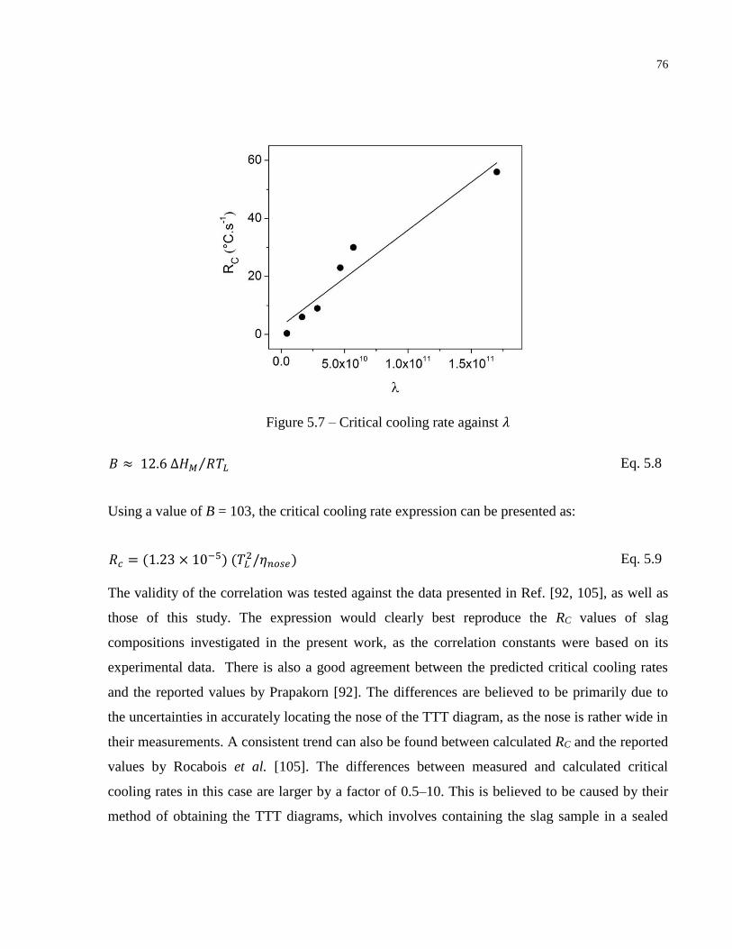
76

Figure 5.7 – Critical cooling rate against 𝜆

𝐵 ≈ 12.6 ∆𝐻𝑀 𝑅𝑇𝐿⁄ Eq. 5.8

Using a value of B = 103, the critical cooling rate expression can be presented as:

𝑅𝑐 = (1.23 × 10−5) (𝑇𝐿2/𝜂𝑛𝑜𝑠𝑒) Eq. 5.9

The validity of the correlation was tested against the data presented in Ref. [92, 105], as well as

those of this study. The expression would clearly best reproduce the RC values of slag

compositions investigated in the present work, as the correlation constants were based on its

experimental data. There is also a good agreement between the predicted critical cooling rates

and the reported values by Prapakorn [92]. The differences are believed to be primarily due to

the uncertainties in accurately locating the nose of the TTT diagram, as the nose is rather wide in

their measurements. A consistent trend can also be found between calculated RC and the reported

values by Rocabois et al. [105]. The differences between measured and calculated critical

cooling rates in this case are larger by a factor of 0.5–10. This is believed to be caused by their

method of obtaining the TTT diagrams, which involves containing the slag sample in a sealed

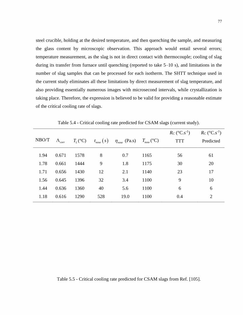
77

steel crucible, holding at the desired temperature, and then quenching the sample, and measuring

the glass content by microscopic observation. This approach would entail several errors;

temperature measurement, as the slag is not in direct contact with thermocouple; cooling of slag

during its transfer from furnace until quenching (reported to take 5–10 s), and limitations in the

number of slag samples that can be processed for each isotherm. The SHTT technique used in

the current study eliminates all these limitations by direct measurement of slag temperature, and

also providing essentially numerous images with microsecond intervals, while crystallization is

taking place. Therefore, the expression is believed to be valid for providing a reasonable estimate

of the critical cooling rate of slags.

Table 5.4 - Critical cooling rate predicted for CSAM slags (current study).

NBO/T

(°C)

(Pa.s)

(°C)

RC (°C.s-1)

TTT

RC (°C.s-1)

Predicted

1.94 0.671 1578 8 0.7 1165 56 61

1.78 0.661 1444 9 1.8 1175 30 20

1.71 0.656 1430 12 2.1 1140 23 17

1.56 0.645 1396 32 3.4 1100 9 10

1.44 0.636 1360 40 5.6 1100 6 6

1.18 0.616 1290 528 19.0 1100 0.4 2

Table 5.5 - Critical cooling rate predicted for CSAM slags from Ref. [105].

Λcorr LT noset snose noseT

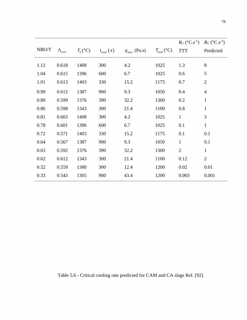
78

NBO/T

(°C)

(Pa.s)

(°C)

RC (°C.s-1)

TTT

RC (°C.s-1)

Predicted

1.12 0.618 1408 300 4.2 1025 1.3 8

1.04 0.615 1396 600 6.7 1025 0.6 5

1.01 0.613 1403 330 15.2 1175 0.7 2

0.99 0.612 1387 900 9.3 1050 0.4 4

0.89 0.599 1376 390 32.2 1300 0.2 1

0.86 0.598 1343 300 21.4 1100 0.8 1

0.81 0.603 1408 300 4.2 1025 1 3

0.78 0.601 1396 600 6.7 1025 0.1 1

0.72 0.571 1403 330 15.2 1175 0.1 0.1

0.64 0.567 1387 900 9.3 1050 1 0.1

0.63 0.592 1376 390 32.2 1300 2 1

0.62 0.612 1343 300 21.4 1100 0.12 2

0.52 0.559 1380 300 12.4 1200 0.02 0.01

0.33 0.543 1305 900 43.4 1200 0.003 0.001

Table 5.6 - Critical cooling rate predicted for CAM and CA slags Ref. [92].


79

NBO/T

(°C)

(Pa.s)

(°C)

RC (°C.s-1)

TTT

RC (°C.s-1)

Predicted

1.27 0.704 1500 6 0.6 1140 59 68

1.13 0.698 1400 8 1.1 1120 37 34

1.07 0.705 1470 5 0.7 1200 54 55

0.92 0.689 1383 8 1.2 1160 28 28

0.84 0.687 1365 18 1.3 1080 16 26

0.66 0.672 1428 5 1 1200 46 32

Figure 5.8 - from TTT vs. predicted.


CR CR

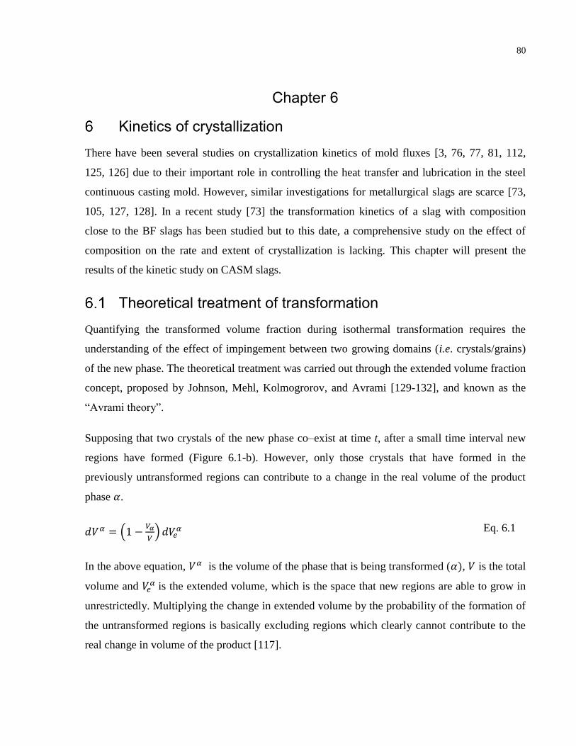
80

Chapter 6

Kinetics of crystallization

There have been several studies on crystallization kinetics of mold fluxes [3, 76, 77, 81, 112,

125, 126] due to their important role in controlling the heat transfer and lubrication in the steel

continuous casting mold. However, similar investigations for metallurgical slags are scarce [73,

105, 127, 128]. In a recent study [73] the transformation kinetics of a slag with composition

close to the BF slags has been studied but to this date, a comprehensive study on the effect of

composition on the rate and extent of crystallization is lacking. This chapter will present the

results of the kinetic study on CASM slags.

Theoretical treatment of transformation

Quantifying the transformed volume fraction during isothermal transformation requires the

understanding of the effect of impingement between two growing domains (i.e. crystals/grains)

of the new phase. The theoretical treatment was carried out through the extended volume fraction

concept, proposed by Johnson, Mehl, Kolmogrorov, and Avrami [129-132], and known as the

“Avrami theory”.

Supposing that two crystals of the new phase co–exist at time t, after a small time interval new

regions have formed (Figure 6.1-b). However, only those crystals that have formed in the

previously untransformed regions can contribute to a change in the real volume of the product

phase 𝛼.

𝑑𝑉𝛼 = (1 −𝑉𝛼

𝑉) 𝑑𝑉𝑒

𝛼 Eq. 6.1

In the above equation, 𝑉𝛼 is the volume of the phase that is being transformed (𝛼), 𝑉 is the total

volume and 𝑉𝑒𝛼 is the extended volume, which is the space that new regions are able to grow in

unrestrictedly. Multiplying the change in extended volume by the probability of the formation of

the untransformed regions is basically excluding regions which clearly cannot contribute to the

real change in volume of the product [117].

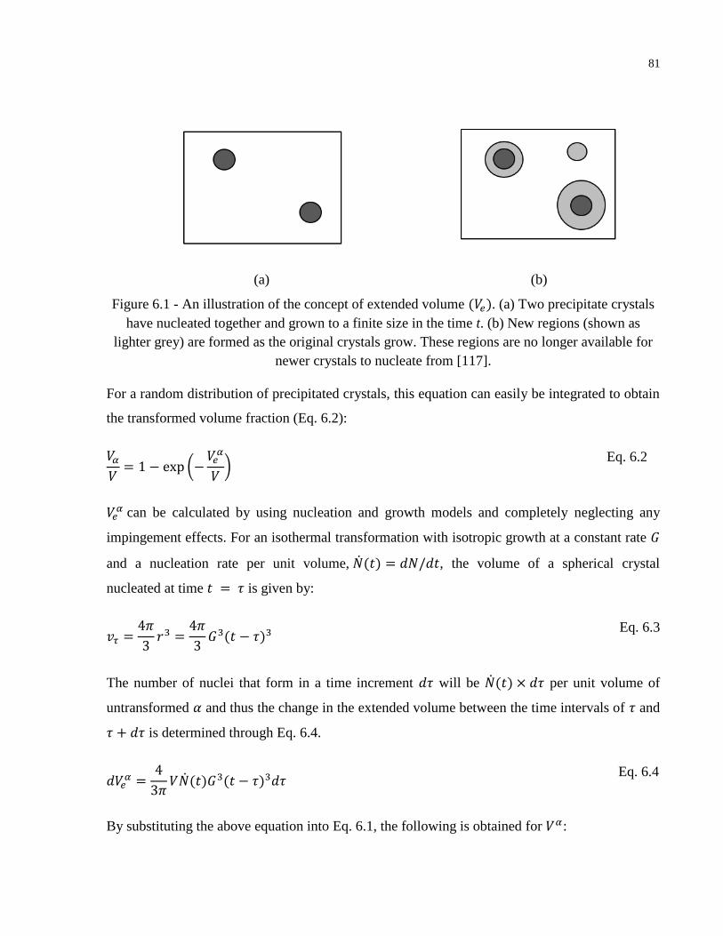
81

(a) (b)

Figure 6.1 - An illustration of the concept of extended volume (𝑉𝑒). (a) Two precipitate crystals

have nucleated together and grown to a finite size in the time t. (b) New regions (shown as

lighter grey) are formed as the original crystals grow. These regions are no longer available for

newer crystals to nucleate from [117].

For a random distribution of precipitated crystals, this equation can easily be integrated to obtain

the transformed volume fraction (Eq. 6.2):

𝑉𝛼

𝑉= 1 − exp (−

𝑉𝑒𝛼

𝑉)

Eq. 6.2

𝑉𝑒𝛼 can be calculated by using nucleation and growth models and completely neglecting any

impingement effects. For an isothermal transformation with isotropic growth at a constant rate 𝐺

and a nucleation rate per unit volume, ��(𝑡) = 𝑑𝑁/𝑑𝑡, the volume of a spherical crystal

nucleated at time 𝑡 = 𝜏 is given by:

𝑣𝜏 =4𝜋

3𝑟3 =

4𝜋

3𝐺3(𝑡 − 𝜏)3

Eq. 6.3

The number of nuclei that form in a time increment 𝑑𝜏 will be ��(𝑡) × 𝑑𝜏 per unit volume of

untransformed 𝛼 and thus the change in the extended volume between the time intervals of 𝜏 and

𝜏 + 𝑑𝜏 is determined through Eq. 6.4.

𝑑𝑉𝑒𝛼 =

4

3𝜋𝑉��(𝑡)𝐺3(𝑡 − 𝜏)3𝑑𝜏

Eq. 6.4

By substituting the above equation into Eq. 6.1, the following is obtained for 𝑉𝛼:

82

𝑑𝑉𝛼 = (4

3𝜋) (1 −

𝑉𝛼

𝑉) 𝑉𝑁(𝑡) 𝐺3(𝑡 − 𝜏)3𝑑𝜏

Eq. 6.5

considering, 𝑋 =𝑉𝛼

𝑉, is obtained:

−𝐿𝑛(1 − 𝑋) =4𝜋

3𝐺3��(𝑡) ∫ (𝑡 − 𝜏)3

𝑡

0

𝑑𝜏 =𝜋

3��(𝑡)𝐺3𝑡4

Eq. 6.6

and therefore at a constant nucleation rate we have:

𝑋 = 1 − exp [−𝜋

3��(𝑡)𝐺3𝑡4] Eq. 6.7

This equation (Eq. 6.7) is known as the Johnson-Mehl-Avrami-Kolmogorov (JMAK) equation.

A simplified form of the above equation is often used (Eq. 6.8).

𝑋 = 1 − exp [−(𝑘𝑡)𝑛] Eq. 6.8

This expression describes the relationship between the transformed volume fraction and time as a

sigmoidal curve. The coefficient K is a kinetic parameter which includes both nucleation and

growth rates. The Avrami exponent, 𝑛, can provide useful information on the mechanism of

transformation. In the following paragraphs, the relationship between 𝑛 and the mechanism of

nucleation and growth will be described.

In the case of transient nucleation rate, if 𝑁(𝑡) is considered a simple function of time, at an

isothermal temperature 𝑁(𝑡) =𝑁0𝑡𝑎 and thus, ��(𝑡) = 𝑎𝑁0𝑡𝑎−1.

The growth mechanism can be either diffusion-controlled or interface-controlled. The former

involves short or long-term diffusion of atoms so that the formation of new phase involves

compositional changes. The interface-controlled growth on the other hand takes place through

local rearrangement of the atoms. In the case of diffusion controlled growth, 𝐺 can be considered

a function of diffusion coefficient and time, 𝐺 = 𝑘 (𝐷/𝑡)1/2. By substituting ��(𝑡) and 𝐺 into

Eq. 6.7 and comparing with Eq. 6.8, we can find:

83

- if a>1, i.e. nucleation rate is increasing with time, n>2.5

- if 1>a>0, i.e. nucleation rate is decreasing with time, 2.5>n>1.5

- if a=1, i.e. nucleation rate is constant with time and n=2.5

- if a=0, i.e. nucleation rate is zero and n=1.5

However, if the growth is interface-controlled, the growth rate, 𝐺, is constant with time,

therefore:

- if a>1, i.e. nucleation rate is increasing with time, n>4

- if 1>a>0, i.e. nucleation rate is decreasing with time, n=4

- if a=1, i.e. nucleation rate is constant with time and 3>n>4

- if a=0, i.e. nucleation rate is zero and n=3

The above is summarized in relation to the Avrami exponent in Table 6.1.

Table 6.1 - Values of the Avrami exponent in relation to geometry and mechanism of growth

[104]

Diffusion-controlled growth n Interface-controlled growth n

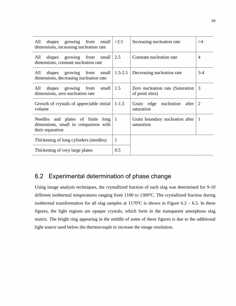
84

All shapes growing from small

dimensions, increasing nucleation rate

>2.5 Increasing nucleation rate >4


dimensions, constant nucleation rate

2.5 Constant nucleation rate 4


dimensions, decreasing nucleation rate

1.5-2.5 Decreasing nucleation rate 3-4


dimensions, zero nucleation rate

1.5 Zero nucleation rate (Saturation

of point sites)

3

Growth of crystals of appreciable initial

volume

1-1.5 Grain edge nucleation after

saturation

2

Needles and plates of finite long

dimensions, small in comparison with

their separation

1 Grain boundary nucleation after

saturation

1

Thickening of long cylinders (needles) 1

Thickening of very large plates 0.5

Experimental determination of phase change

Using image analysis techniques, the crystallized fraction of each slag was determined for 9-10

different isothermal temperatures ranging from 1100 to 1300ºC. The crystallized fraction during

isothermal transformation for all slag samples at 1170ºC is shown in Figure 6.2 – 6.5. In these

figures, the light regions are opaque crystals, which form in the transparent amorphous slag

matrix. The bright ring appearing in the middle of some of these figures is due to the additional

light source used below the thermocouple to increase the image resolution.

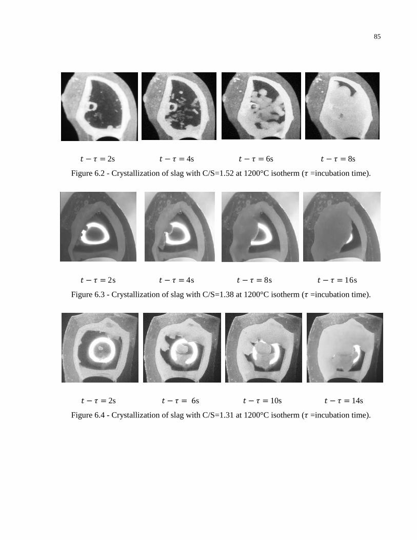
85

𝑡 − 𝜏 = 2s 𝑡 − 𝜏 = 4s 𝑡 − 𝜏 = 6s 𝑡 − 𝜏 = 8s

Figure 6.2 - Crystallization of slag with C/S=1.52 at 1200°C isotherm (𝜏 =incubation time).

𝑡 − 𝜏 = 2s 𝑡 − 𝜏 = 4s 𝑡 − 𝜏 = 8s 𝑡 − 𝜏 = 16s


𝑡 − 𝜏 = 2s 𝑡 − 𝜏 = 6s 𝑡 − 𝜏 = 10s 𝑡 − 𝜏 = 14s


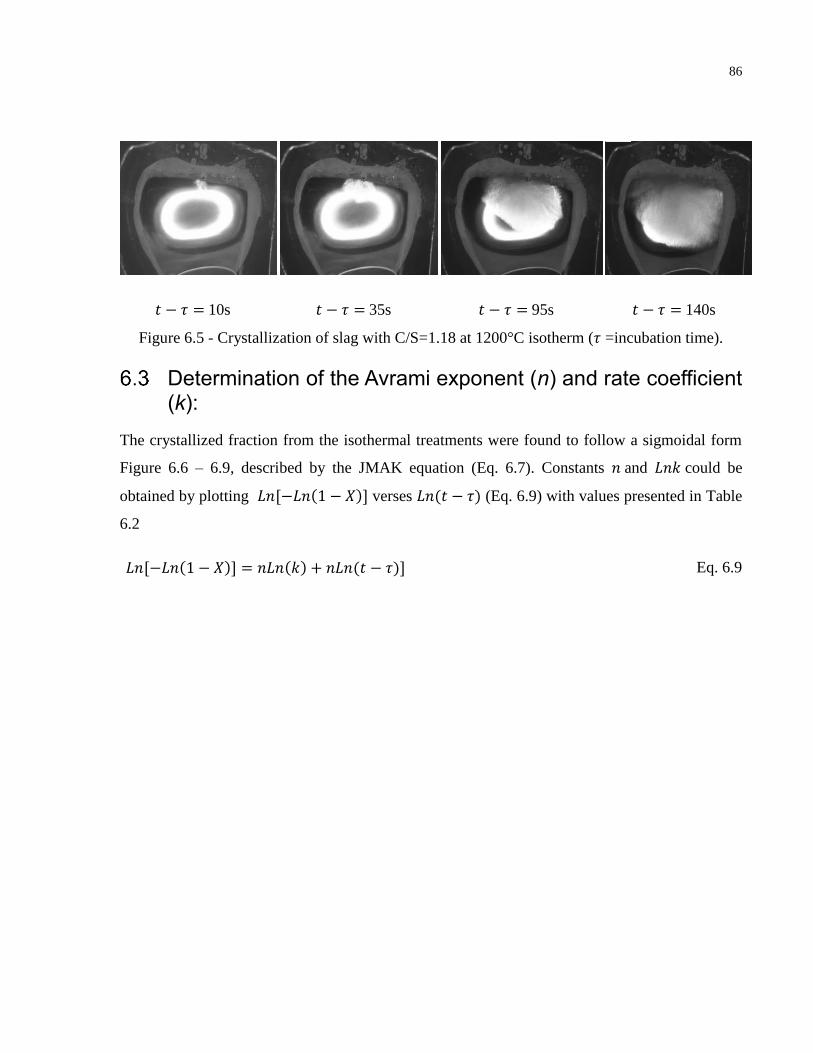
86

𝑡 − 𝜏 = 10s 𝑡 − 𝜏 = 35s 𝑡 − 𝜏 = 95s 𝑡 − 𝜏 = 140s


Determination of the Avrami exponent (n) and rate coefficient (k):

The crystallized fraction from the isothermal treatments were found to follow a sigmoidal form

Figure 6.6 – 6.9, described by the JMAK equation (Eq. 6.7). Constants 𝑛 and 𝐿𝑛𝑘 could be

obtained by plotting 𝐿𝑛[−𝐿𝑛(1 − 𝑋)] verses 𝐿𝑛(𝑡 − 𝜏) (Eq. 6.9) with values presented in Table

6.2

𝐿𝑛[−𝐿𝑛(1 − 𝑋)] = 𝑛𝐿𝑛(𝑘) + 𝑛𝐿𝑛(𝑡 − 𝜏)] Eq. 6.9

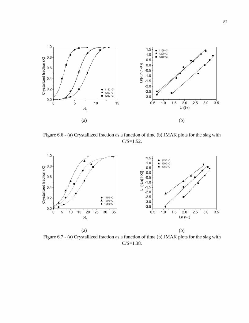
87

0 5 10 150.0

0.2

0.4

0.6

0.8

1.0

1150C

1200C

1250C

Cry

sta

llized fra

ction (

X)

t-t0

0.5 1.0 1.5 2.0 2.5 3.0 3.5

-3.0

-2.5

-2.0

-1.5

-1.0

-0.5

0.0

0.5

1.0

1.5

Ln[-

Ln(1

-X)]

1150C

1200C

1250C

Ln(t-

(a) (b)


C/S=1.52.

0 5 10 15 20 25 30 350.0

0.2

0.4

0.6

0.8

1.0

1150C

1200C

1250C Cry

sta

llized fra

ction (

X)

t-t0

0.5 1.0 1.5 2.0 2.5 3.0 3.5

-3.5

-3.0

-2.5

-2.0

-1.5

-1.0

-0.5

0.0

0.5

1.0

1.5

Ln[-

Ln(1

-X)]

1150C

1200C

1250C

Ln (t-)

(a) (b)


C/S=1.38.

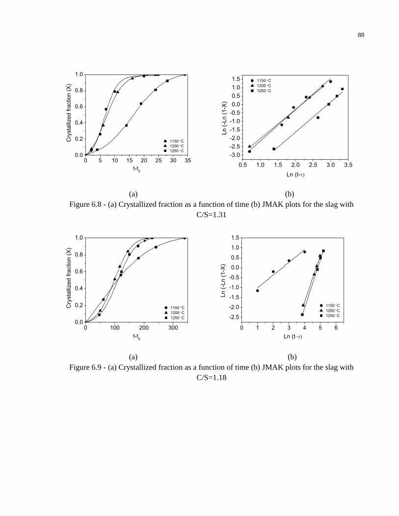
88

0 5 10 15 20 25 30 350.0

0.2

0.4

0.6

0.8

1.0

1150C

1200C

1250C

Cry

sta

llized fra

ction (

X)

t-t0

0.5 1.0 1.5 2.0 2.5 3.0 3.5

-3.0

-2.5

-2.0

-1.5

-1.0

-0.5

0.0

0.5

1.0

1.5 1150C

1200C

1250C

Ln (

-Ln (

1-X

)

Ln (t-

(a) (b)


C/S=1.31

0 100 200 3000.0

0.2

0.4

0.6

0.8

1.0

1150C

1200C

1250C

Cry

sta

llized fra

ction (

X)

t-t0

0 1 2 3 4 5 6

-2.5

-2.0

-1.5

-1.0

-0.5

0.0

0.5

1.0

1.5

1150C

1200C

1250C

Ln (

-Ln (

1-X

)

Ln (t

(a) (b)


C/S=1.18

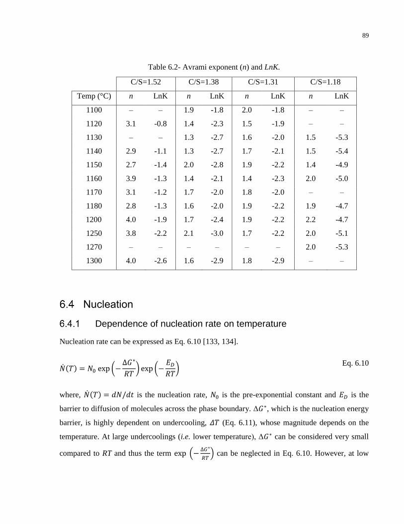
89

Table 6.2- Avrami exponent (n) and LnK.

C/S=1.52 C/S=1.38 C/S=1.31 C/S=1.18

Temp (°C) n LnK n LnK n LnK n LnK

1100 ‒ ‒ 1.9 -1.8 2.0 -1.8 ‒ ‒

1120 3.1 -0.8 1.4 -2.3 1.5 -1.9 ‒ ‒

1130 ‒ ‒ 1.3 -2.7 1.6 -2.0 1.5 -5.3

1140 2.9 -1.1 1.3 -2.7 1.7 -2.1 1.5 -5.4

1150 2.7 -1.4 2.0 -2.8 1.9 -2.2 1.4 -4.9

1160 3.9 -1.3 1.4 -2.1 1.4 -2.3 2.0 -5.0

1170 3.1 -1.2 1.7 -2.0 1.8 -2.0 ‒ ‒

1180 2.8 -1.3 1.6 -2.0 1.9 -2.2 1.9 -4.7

1200 4.0 -1.9 1.7 -2.4 1.9 -2.2 2.2 -4.7

1250 3.8 -2.2 2.1 -3.0 1.7 -2.2 2.0 -5.1

1270 ‒ ‒ ‒ ‒ ‒ ‒ 2.0 -5.3

1300 4.0 -2.6 1.6 -2.9 1.8 -2.9 ‒ ‒

Nucleation

Dependence of nucleation rate on temperature

Nucleation rate can be expressed as Eq. 6.10 [133, 134].

��(𝑇) = 𝑁0 exp (−∆𝐺∗

𝑅𝑇) exp (−

𝐸𝐷

𝑅𝑇)

Eq. 6.10

where, ��(𝑇) = 𝑑𝑁/𝑑𝑡 is the nucleation rate, 𝑁0 is the pre-exponential constant and 𝐸𝐷 is the

barrier to diffusion of molecules across the phase boundary. Δ𝐺∗, which is the nucleation energy

barrier, is highly dependent on undercooling, 𝛥𝑇 (Eq. 6.11), whose magnitude depends on the

temperature. At large undercoolings (i.e. lower temperature), Δ𝐺∗ can be considered very small

compared to RT and thus the term exp (−∆𝐺∗

𝑅𝑇) can be neglected in Eq. 6.10. However, at low

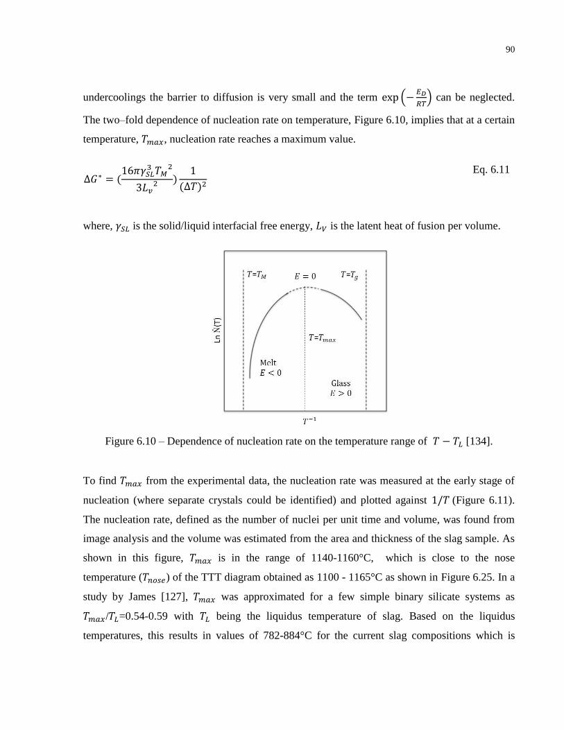
90

undercoolings the barrier to diffusion is very small and the term exp (−𝐸𝐷

𝑅𝑇) can be neglected.

The two–fold dependence of nucleation rate on temperature, Figure 6.10, implies that at a certain

temperature, 𝑇𝑚𝑎𝑥, nucleation rate reaches a maximum value.

∆𝐺∗ = (16𝜋𝛾𝑆𝐿

3 𝑇𝑀2

3𝐿𝑣2 )

1

(∆𝑇)2

Eq. 6.11

where, 𝛾𝑆𝐿 is the solid/liquid interfacial free energy, 𝐿𝑉 is the latent heat of fusion per volume.

Figure 6.10 – Dependence of nucleation rate on the temperature range of 𝑇 − 𝑇𝐿 [134].

To find 𝑇𝑚𝑎𝑥 from the experimental data, the nucleation rate was measured at the early stage of

nucleation (where separate crystals could be identified) and plotted against 1/𝑇 (Figure 6.11).

The nucleation rate, defined as the number of nuclei per unit time and volume, was found from

image analysis and the volume was estimated from the area and thickness of the slag sample. As

shown in this figure, 𝑇𝑚𝑎𝑥 is in the range of 1140-1160°C, which is close to the nose

temperature (𝑇𝑛𝑜𝑠𝑒) of the TTT diagram obtained as 1100 - 1165°C as shown in Figure 6.25. In a

study by James [127], 𝑇𝑚𝑎𝑥 was approximated for a few simple binary silicate systems as

𝑇𝑚𝑎𝑥/𝑇𝐿=0.54-0.59 with 𝑇𝐿 being the liquidus temperature of slag. Based on the liquidus

temperatures, this results in values of 782-884°C for the current slag compositions which is

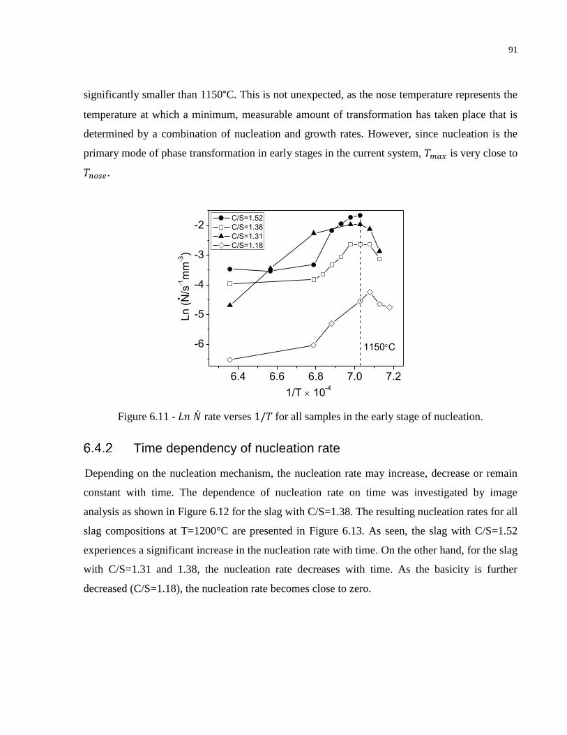
91

significantly smaller than 1150°C. This is not unexpected, as the nose temperature represents the

temperature at which a minimum, measurable amount of transformation has taken place that is

determined by a combination of nucleation and growth rates. However, since nucleation is the

primary mode of phase transformation in early stages in the current system, 𝑇𝑚𝑎𝑥 is very close to

𝑇𝑛𝑜𝑠𝑒.

6.4 6.6 6.8 7.0 7.2

-6

-5

-4

-3

-2 C/S=1.52

C/S=1.38

C/S=1.31

C/S=1.18

Ln (

N/s

-1m

m-3)

1/T 10-4

1150C

Figure 6.11 - 𝐿𝑛 �� rate verses 1/𝑇 for all samples in the early stage of nucleation.

Time dependency of nucleation rate

Depending on the nucleation mechanism, the nucleation rate may increase, decrease or remain

constant with time. The dependence of nucleation rate on time was investigated by image

analysis as shown in Figure 6.12 for the slag with C/S=1.38. The resulting nucleation rates for all

slag compositions at T=1200°C are presented in Figure 6.13. As seen, the slag with C/S=1.52

experiences a significant increase in the nucleation rate with time. On the other hand, for the slag

with C/S=1.31 and 1.38, the nucleation rate decreases with time. As the basicity is further

decreased (C/S=1.18), the nucleation rate becomes close to zero.

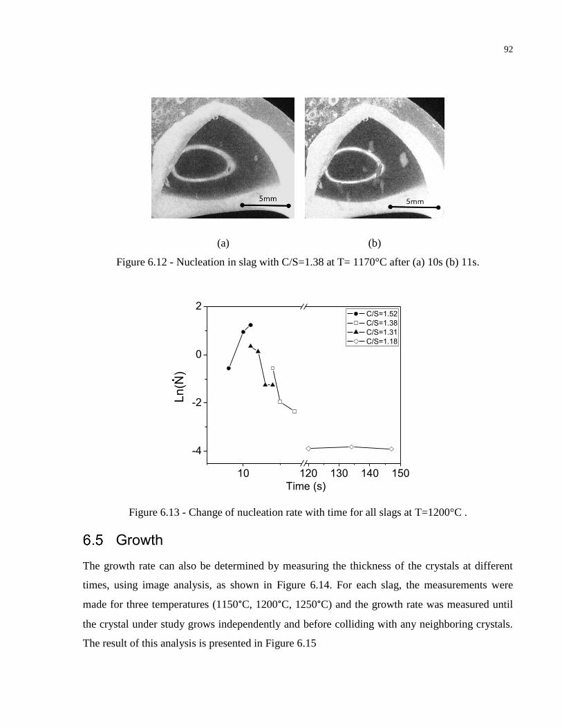
92

(a)

(b)

Figure 6.12 - Nucleation in slag with C/S=1.38 at T= 1170°C after (a) 10s (b) 11s.

10 120 130 140 150

-4

-2

0

2

Ln

(N)

Time (s)

C/S=1.52

C/S=1.38

C/S=1.31

C/S=1.18

Figure 6.13 - Change of nucleation rate with time for all slags at T=1200°C .

Growth

The growth rate can also be determined by measuring the thickness of the crystals at different

times, using image analysis, as shown in Figure 6.14. For each slag, the measurements were

made for three temperatures (1150°C, 1200°C, 1250°C) and the growth rate was measured until

the crystal under study grows independently and before colliding with any neighboring crystals.

The result of this analysis is presented in Figure 6.15

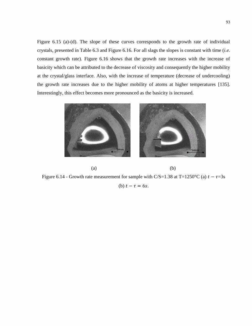
93

Figure 6.15 (a)-(d). The slope of these curves corresponds to the growth rate of individual

crystals, presented in Table 6.3 and Figure 6.16. For all slags the slopes is constant with time (i.e.

constant growth rate). Figure 6.16 shows that the growth rate increases with the increase of

basicity which can be attributed to the decrease of viscosity and consequently the higher mobility

at the crystal/glass interface. Also, with the increase of temperature (decrease of undercooling)

the growth rate increases due to the higher mobility of atoms at higher temperatures [135].

Interestingly, this effect becomes more pronounced as the basicity is increased.

(a) (b)

Figure 6.14 - Growth rate measurement for sample with C/S=1.38 at T=1250°C (a) 𝑡 − 𝜏=3s

(b) 𝑡 − 𝜏 = 6𝑠.

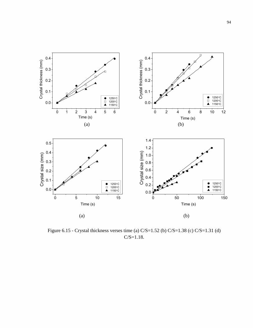
94

0 1 2 3 4 5 6

0.0

0.1

0.2

0.3

0.4

1250C

1200C

1150C

Cry

sta

l th

ickness (

mm

)

Time (s)

(a)

0 2 4 6 8 10 12

0.0

0.1

0.2

0.3

0.4

1250C

1200C

1150C

Cry

sta

l th

ickness (

mm

)

Time (s)

(b)

0 5 10 15

0.0

0.1

0.2

0.3

0.4

0.5

1250C

1200C

1150C

Cry

sta

l siz

e (

mm

)

Time (s)

0 50 100 150

0.0

0.2

0.4

0.6

0.8

1.0

1.2

1.4

1250C

1200C

1150C

Cry

sta

l siz

e (

mm

)

Time (s)

(a) (b)

Figure 6.15 - Crystal thickness verses time (a) C/S=1.52 (b) C/S=1.38 (c) C/S=1.31 (d)

C/S=1.18.

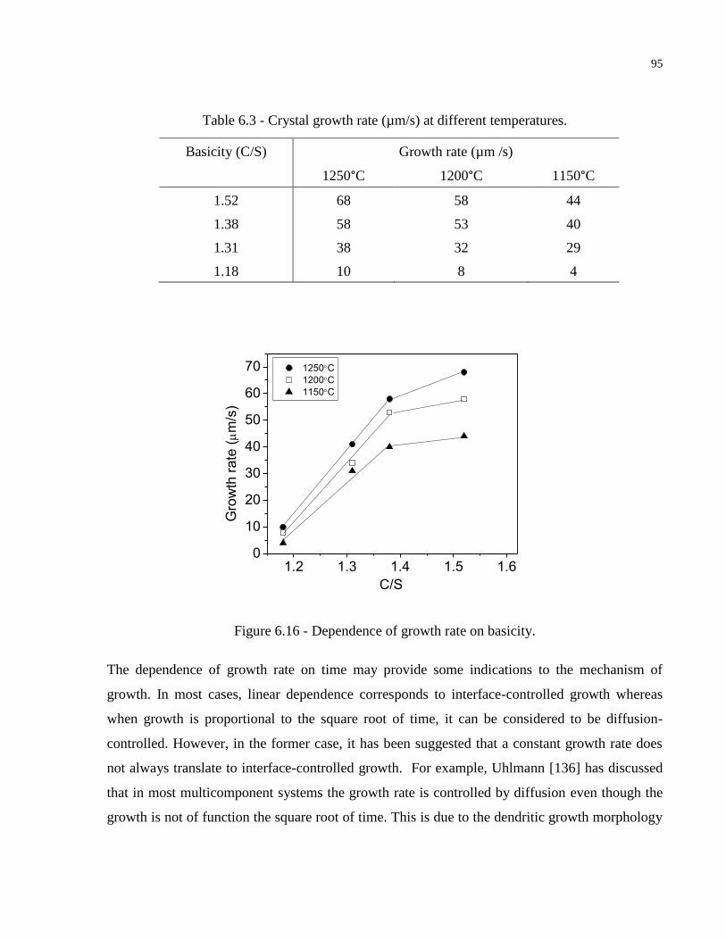
95

Table 6.3 - Crystal growth rate (µm/s) at different temperatures.

Basicity (C/S) Growth rate (µm /s)

1250°C 1200°C 1150°C

1.52 68 58 44

1.38 58 53 40

1.31 38 32 29

1.18 10 8 4

1.2 1.3 1.4 1.5 1.60

10

20

30

40

50

60

70 1250C

1200C

1150C

Gro

wth

rate

(m

/s)

C/S

Figure 6.16 - Dependence of growth rate on basicity.

The dependence of growth rate on time may provide some indications to the mechanism of

growth. In most cases, linear dependence corresponds to interface-controlled growth whereas

when growth is proportional to the square root of time, it can be considered to be diffusion-

controlled. However, in the former case, it has been suggested that a constant growth rate does

not always translate to interface-controlled growth. For example, Uhlmann [136] has discussed

that in most multicomponent systems the growth rate is controlled by diffusion even though the

growth is not of function the square root of time. This is due to the dendritic growth morphology

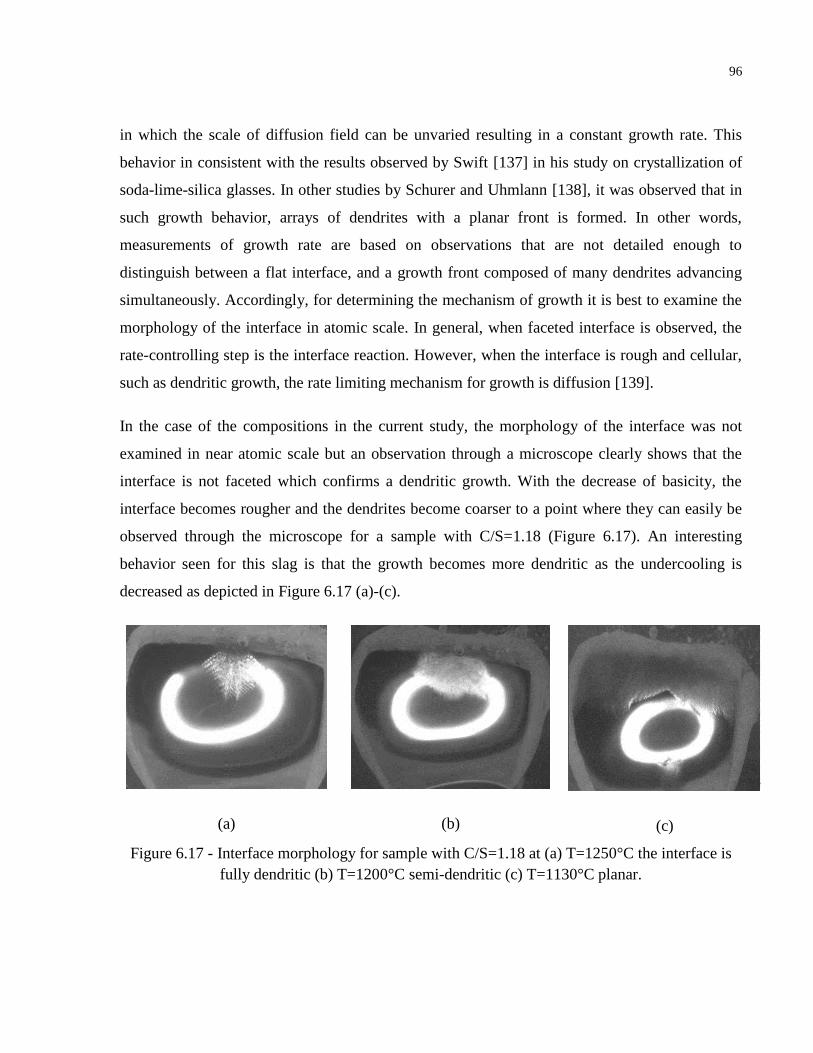
96

in which the scale of diffusion field can be unvaried resulting in a constant growth rate. This

behavior in consistent with the results observed by Swift [137] in his study on crystallization of

soda-lime-silica glasses. In other studies by Schurer and Uhmlann [138], it was observed that in

such growth behavior, arrays of dendrites with a planar front is formed. In other words,

measurements of growth rate are based on observations that are not detailed enough to

distinguish between a flat interface, and a growth front composed of many dendrites advancing

simultaneously. Accordingly, for determining the mechanism of growth it is best to examine the

morphology of the interface in atomic scale. In general, when faceted interface is observed, the

rate-controlling step is the interface reaction. However, when the interface is rough and cellular,

such as dendritic growth, the rate limiting mechanism for growth is diffusion [139].

In the case of the compositions in the current study, the morphology of the interface was not

examined in near atomic scale but an observation through a microscope clearly shows that the

interface is not faceted which confirms a dendritic growth. With the decrease of basicity, the

interface becomes rougher and the dendrites become coarser to a point where they can easily be

observed through the microscope for a sample with C/S=1.18 (Figure 6.17). An interesting

behavior seen for this slag is that the growth becomes more dendritic as the undercooling is

decreased as depicted in Figure 6.17 (a)-(c).

(a)

(b)

(c)

Figure 6.17 - Interface morphology for sample with C/S=1.18 at (a) T=1250°C the interface is

fully dendritic (b) T=1200°C semi-dendritic (c) T=1130°C planar.

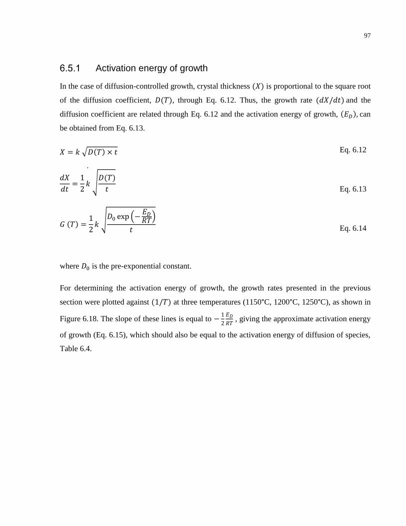
97

Activation energy of growth

In the case of diffusion-controlled growth, crystal thickness (𝑋) is proportional to the square root

of the diffusion coefficient, 𝐷(𝑇), through Eq. 6.12. Thus, the growth rate (𝑑𝑋/𝑑𝑡) and the

diffusion coefficient are related through Eq. 6.12 and the activation energy of growth, (𝐸𝐷), can

be obtained from Eq. 6.13.

𝑋 = 𝑘 √𝐷(𝑇) × 𝑡 Eq. 6.12

𝑑𝑋

𝑑𝑡=

1

2𝑘 √

𝐷(𝑇)

𝑡

Eq. 6.13

𝐺 (𝑇) =1

2𝑘

√𝐷0 exp (−𝐸𝐷

𝑅𝑇)

𝑡

Eq. 6.14

where 𝐷0 is the pre-exponential constant.

For determining the activation energy of growth, the growth rates presented in the previous

section were plotted against (1/𝑇) at three temperatures (1150°C, 1200°C, 1250°C), as shown in

Figure 6.18. The slope of these lines is equal to −1

2

𝐸𝐷

𝑅𝑇 , giving the approximate activation energy

of growth (Eq. 6.15), which should also be equal to the activation energy of diffusion of species,

Table 6.4.

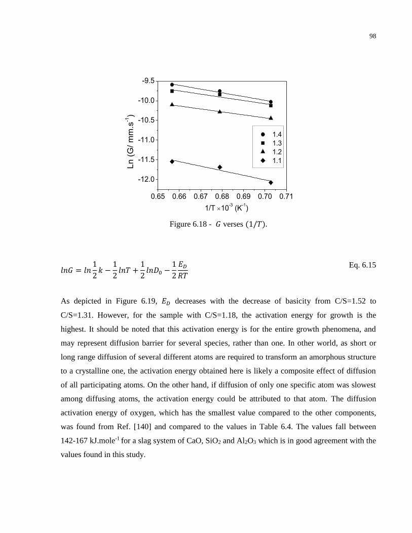
98

0.65 0.66 0.67 0.68 0.69 0.70 0.71

-12.0

-11.5

-11.0

-10.5

-10.0

-9.5

1.4

1.3

1.2

1.1

Ln

(G

/ m

m.s

-1)

1/T 10-3 (K

-1)

Figure 6.18 - 𝐺 verses (1/𝑇).

𝑙𝑛𝐺 = 𝑙𝑛1

2𝑘 −

1

2𝑙𝑛𝑇 +

1

2𝑙𝑛𝐷0 −

1

2

𝐸𝐷

𝑅𝑇

Eq. 6.15

As depicted in Figure 6.19, 𝐸𝐷 decreases with the decrease of basicity from C/S=1.52 to

C/S=1.31. However, for the sample with C/S=1.18, the activation energy for growth is the

highest. It should be noted that this activation energy is for the entire growth phenomena, and

may represent diffusion barrier for several species, rather than one. In other world, as short or

long range diffusion of several different atoms are required to transform an amorphous structure

to a crystalline one, the activation energy obtained here is likely a composite effect of diffusion

of all participating atoms. On the other hand, if diffusion of only one specific atom was slowest

among diffusing atoms, the activation energy could be attributed to that atom. The diffusion

activation energy of oxygen, which has the smallest value compared to the other components,

was found from Ref. [140] and compared to the values in Table 6.4. The values fall between

142-167 kJ.mole-1 for a slag system of CaO, SiO2 and Al2O3 which is in good agreement with the

values found in this study.

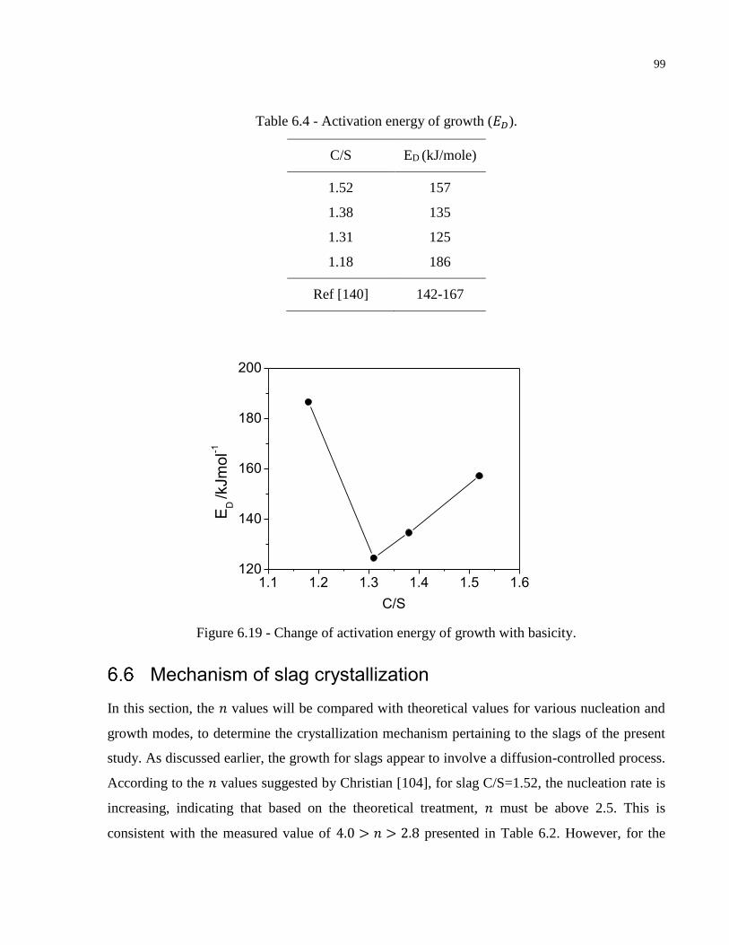
99

Table 6.4 - Activation energy of growth (𝐸𝐷).

C/S ED (kJ/mole)

1.52 157

1.38 135

1.31 125

1.18 186

Ref [140] 142-167

1.1 1.2 1.3 1.4 1.5 1.6120

140

160

180

200

ED

/kJm

ol-1

C/S

Figure 6.19 - Change of activation energy of growth with basicity.

Mechanism of slag crystallization

In this section, the 𝑛 values will be compared with theoretical values for various nucleation and

growth modes, to determine the crystallization mechanism pertaining to the slags of the present

study. As discussed earlier, the growth for slags appear to involve a diffusion-controlled process.

According to the 𝑛 values suggested by Christian [104], for slag C/S=1.52, the nucleation rate is

increasing, indicating that based on the theoretical treatment, 𝑛 must be above 2.5. This is

consistent with the measured value of 4.0 > 𝑛 > 2.8 presented in Table 6.2. However, for the

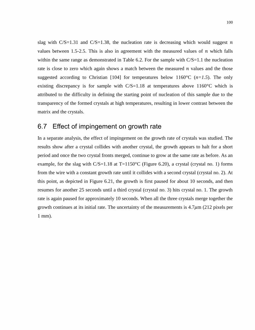
100

slag with C/S=1.31 and C/S=1.38, the nucleation rate is decreasing which would suggest 𝑛

values between 1.5-2.5. This is also in agreement with the measured values of 𝑛 which falls

within the same range as demonstrated in Table 6.2. For the sample with C/S=1.1 the nucleation

rate is close to zero which again shows a match between the measured 𝑛 values and the those

suggested according to Christian [104] for temperatures below 1160°C (n=1.5). The only

existing discrepancy is for sample with C/S=1.18 at temperatures above 1160°C which is

attributed to the difficulty in defining the starting point of nucleation of this sample due to the

transparency of the formed crystals at high temperatures, resulting in lower contrast between the

matrix and the crystals.

Effect of impingement on growth rate

In a separate analysis, the effect of impingement on the growth rate of crystals was studied. The

results show after a crystal collides with another crystal, the growth appears to halt for a short

period and once the two crystal fronts merged, continue to grow at the same rate as before. As an

example, for the slag with C/S=1.18 at T=1150°C (Figure 6.20), a crystal (crystal no. 1) forms

from the wire with a constant growth rate until it collides with a second crystal (crystal no. 2). At

this point, as depicted in Figure 6.21, the growth is first paused for about 10 seconds, and then

resumes for another 25 seconds until a third crystal (crystal no. 3) hits crystal no. 1. The growth

rate is again paused for approximately 10 seconds. When all the three crystals merge together the

growth continues at its initial rate. The uncertainty of the measurements is 4.7𝜇m (212 pixels per

1 mm).

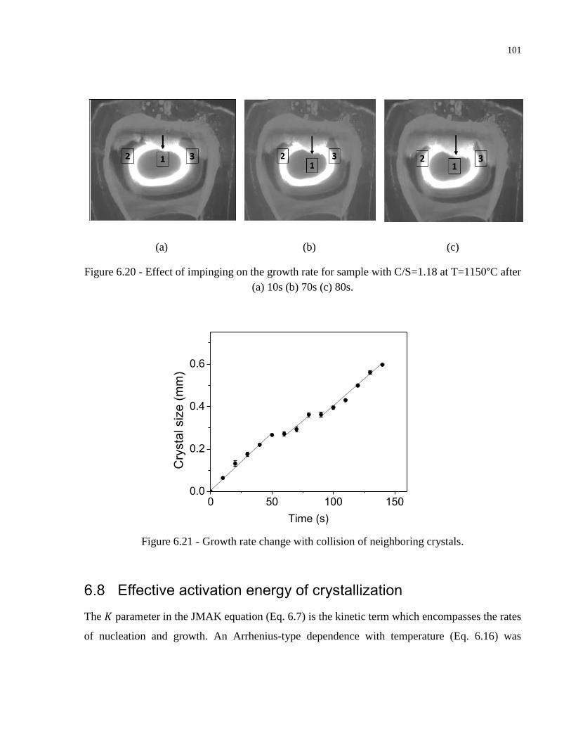
101

(a) (b) (c)

Figure 6.20 - Effect of impinging on the growth rate for sample with C/S=1.18 at T=1150°C after

(a) 10s (b) 70s (c) 80s.

0 50 100 1500.0

0.2

0.4

0.6

Cry

sta

l siz

e (

mm

)

Time (s)

Figure 6.21 - Growth rate change with collision of neighboring crystals.

Effective activation energy of crystallization

The 𝐾 parameter in the JMAK equation (Eq. 6.7) is the kinetic term which encompasses the rates

of nucleation and growth. An Arrhenius-type dependence with temperature (Eq. 6.16) was

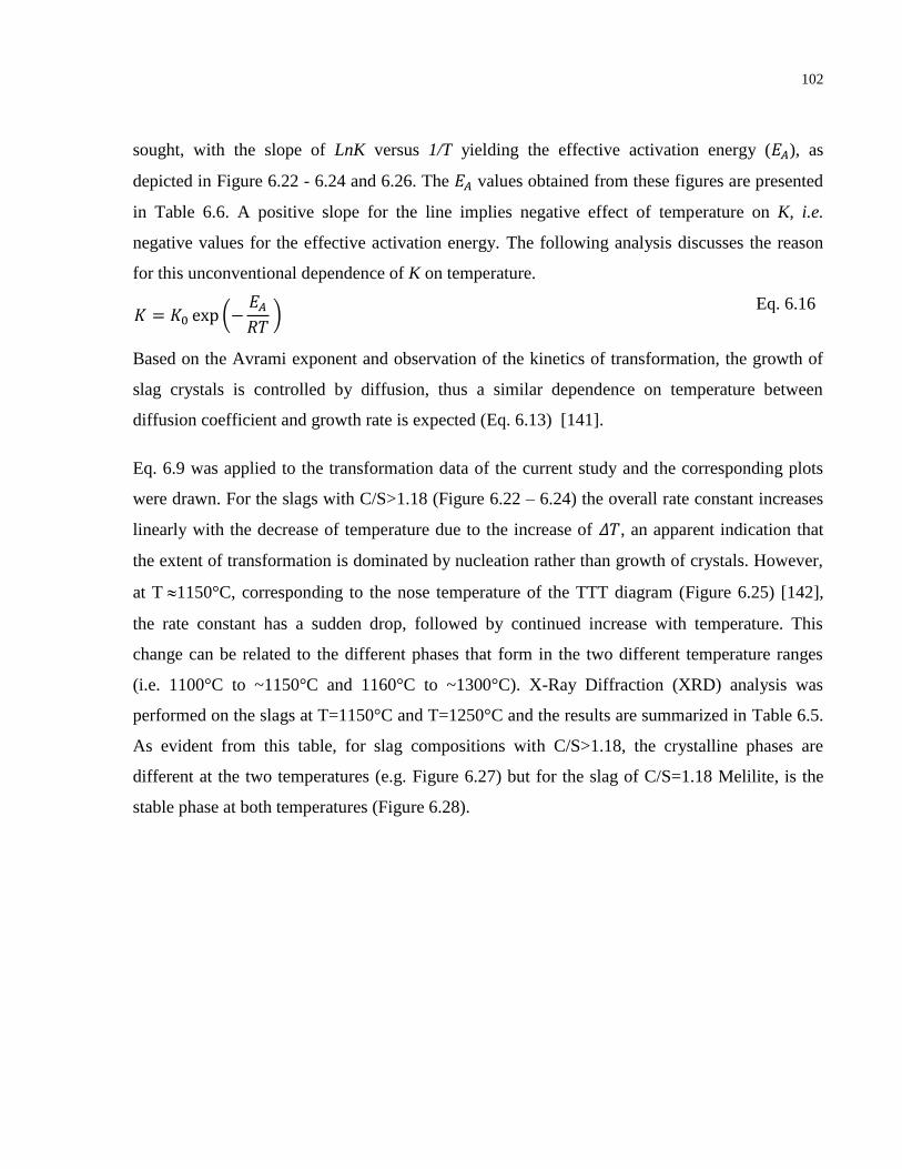
102

sought, with the slope of LnK versus 1/T yielding the effective activation energy (𝐸𝐴), as

depicted in Figure 6.22 - 6.24 and 6.26. The 𝐸𝐴 values obtained from these figures are presented

in Table 6.6. A positive slope for the line implies negative effect of temperature on K, i.e.

negative values for the effective activation energy. The following analysis discusses the reason

for this unconventional dependence of K on temperature.

𝐾 = 𝐾0 exp (−𝐸𝐴

𝑅𝑇 )

Eq. 6.16

Based on the Avrami exponent and observation of the kinetics of transformation, the growth of

slag crystals is controlled by diffusion, thus a similar dependence on temperature between

diffusion coefficient and growth rate is expected (Eq. 6.13) [141].

Eq. 6.9 was applied to the transformation data of the current study and the corresponding plots

were drawn. For the slags with C/S>1.18 (Figure 6.22 – 6.24) the overall rate constant increases

linearly with the decrease of temperature due to the increase of 𝛥𝑇, an apparent indication that

the extent of transformation is dominated by nucleation rather than growth of crystals. However,

at T1150°C, corresponding to the nose temperature of the TTT diagram (Figure 6.25) [142],

the rate constant has a sudden drop, followed by continued increase with temperature. This

change can be related to the different phases that form in the two different temperature ranges

(i.e. 1100°C to ~1150°C and 1160°C to ~1300°C). X-Ray Diffraction (XRD) analysis was

performed on the slags at T=1150°C and T=1250°C and the results are summarized in Table 6.5.

As evident from this table, for slag compositions with C/S>1.18, the crystalline phases are

different at the two temperatures (e.g. Figure 6.27) but for the slag of C/S=1.18 Melilite, is the

stable phase at both temperatures (Figure 6.28).

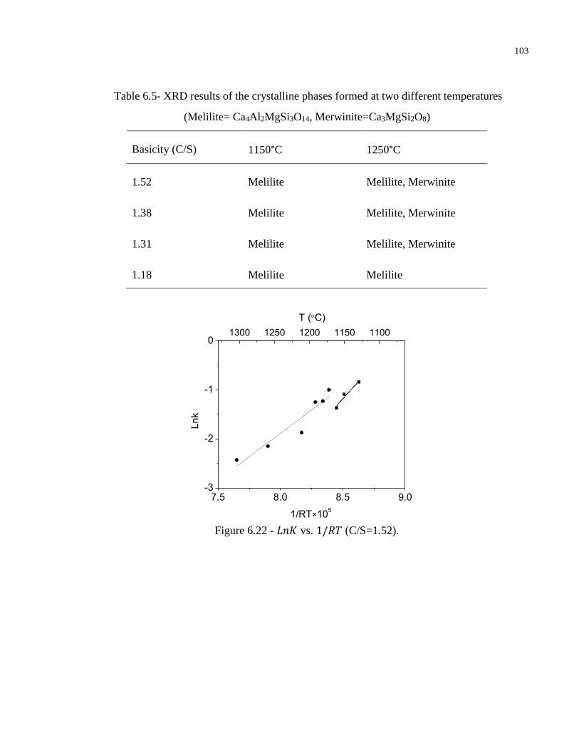
103

Table 6.5- XRD results of the crystalline phases formed at two different temperatures

(Melilite= Ca4Al2MgSi3O14, Merwinite=Ca3MgSi2O8)

Basicity (C/S) 1150°C 1250°C

1.52 Melilite Melilite, Merwinite



1.18 Melilite Melilite

7.5 8.0 8.5 9.0-3

-2

-1

0

T (C)

Lnk

1/RT×105

1300 1250 1200 1150 1100

Figure 6.22 - 𝐿𝑛𝐾 vs. 1/𝑅𝑇 (C/S=1.52).

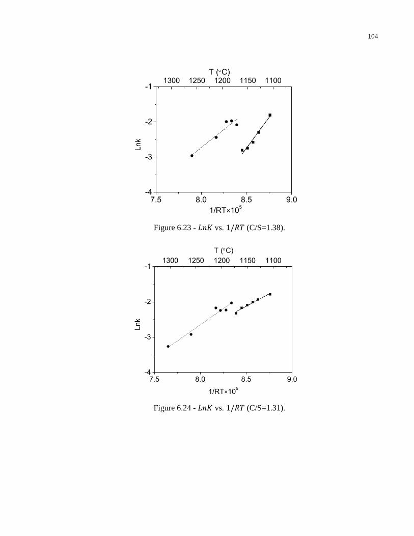
104

7.5 8.0 8.5 9.0-4

-3

-2

-1

T (C)

Ln

k

1/RT×105

1300 1250 1200 1150 1100


7.5 8.0 8.5 9.0-4

-3

-2

-1

T (C)

Lnk

1/RT×105

1300 1250 1200 1150 1100


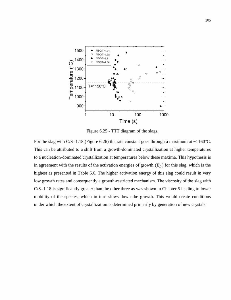
105

1 10 100 1000

900

1000

1100

1200

1300

1400

1500 NBO/T=1.94

NBO/T=1.78

NBO/T=1.71

NBO/T=1.56

Tem

pe

ratu

re (C

)

Time (s)

T=1150C

Figure 6.25 - TTT diagram of the slags.

For the slag with C/S=1.18 (Figure 6.26) the rate constant goes through a maximum at ~1160°C.

This can be attributed to a shift from a growth-dominated crystallization at higher temperatures

to a nucleation-dominated crystallization at temperatures below these maxima. This hypothesis is

in agreement with the results of the activation energies of growth (𝐸𝐷) for this slag, which is the

highest as presented in Table 6.6. The higher activation energy of this slag could result in very

low growth rates and consequently a growth-restricted mechanism. The viscosity of the slag with

C/S=1.18 is significantly greater than the other three as was shown in Chapter 5 leading to lower

mobility of the species, which in turn slows down the growth. This would create conditions

under which the extent of crystallization is determined primarily by generation of new crystals.

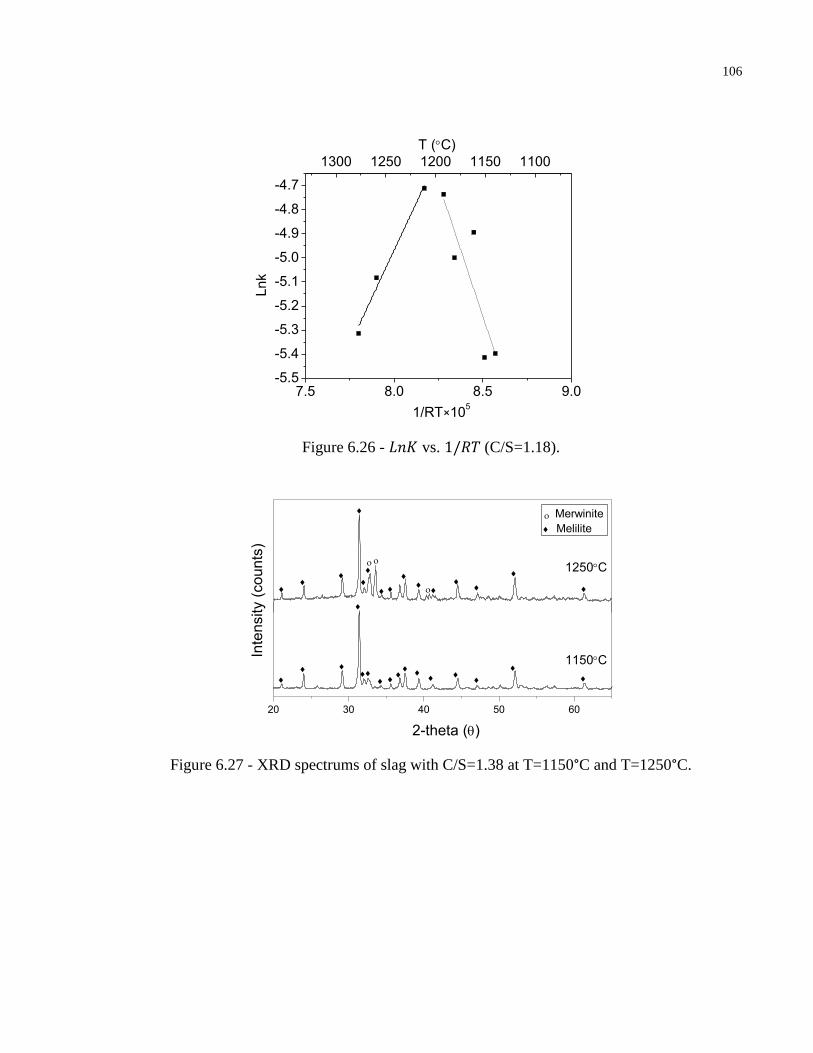
106

7.5 8.0 8.5 9.0-5.5

-5.4

-5.3

-5.2

-5.1

-5.0

-4.9

-4.8

-4.7

T (C)

Lnk

1/RT×105

1300 1250 1200 1150 1100


20 30 40 50 60

2-theta ()

1150C

1250C

Merwinite

Inte

nsity (

co

un

ts)

Melilite

Figure 6.27 - XRD spectrums of slag with C/S=1.38 at T=1150°C and T=1250°C.

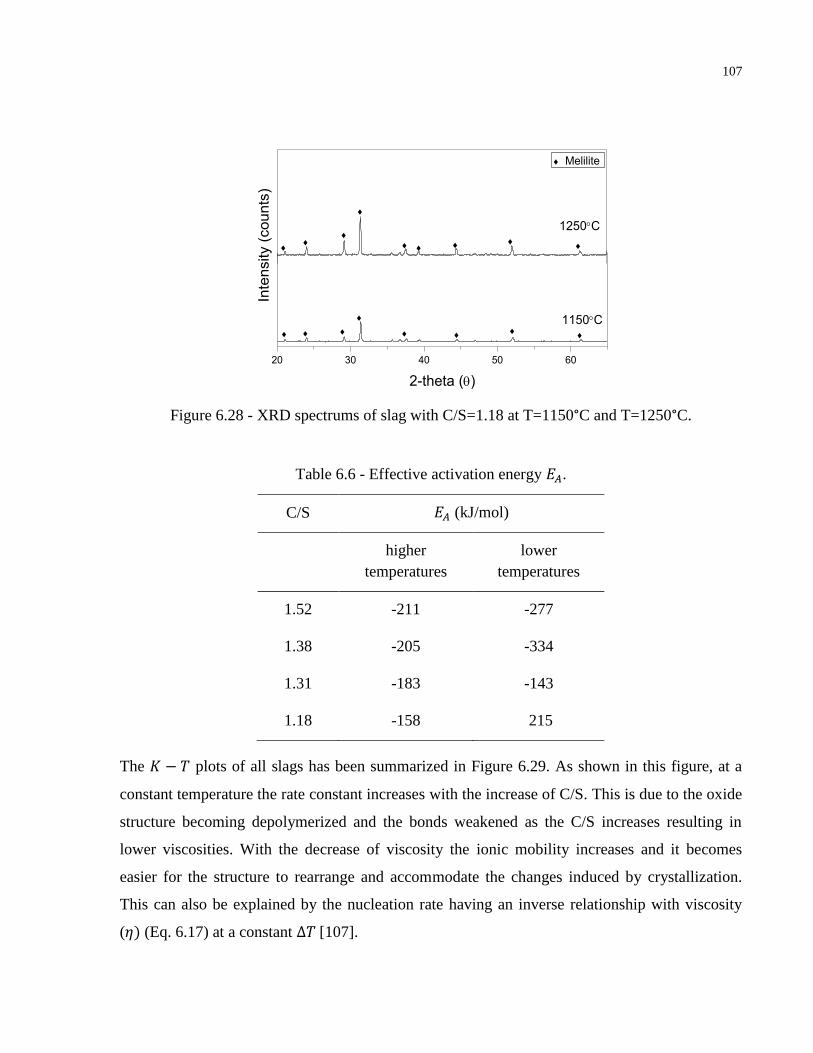
107

20 30 40 50 60

1150C

2-theta ()

Melilite

1250C

Inte

nsity (

counts

)

Figure 6.28 - XRD spectrums of slag with C/S=1.18 at T=1150°C and T=1250°C.

Table 6.6 - Effective activation energy 𝐸𝐴.

C/S 𝐸𝐴 (kJ/mol)

higher

temperatures

lower

temperatures

1.52 -211 -277

1.38 -205 -334

1.31 -183 -143

1.18 -158 215

The 𝐾 − 𝑇 plots of all slags has been summarized in Figure 6.29. As shown in this figure, at a

constant temperature the rate constant increases with the increase of C/S. This is due to the oxide

structure becoming depolymerized and the bonds weakened as the C/S increases resulting in

lower viscosities. With the decrease of viscosity the ionic mobility increases and it becomes

easier for the structure to rearrange and accommodate the changes induced by crystallization.

This can also be explained by the nucleation rate having an inverse relationship with viscosity

(𝜂) (Eq. 6.17) at a constant ∆𝑇 [107].

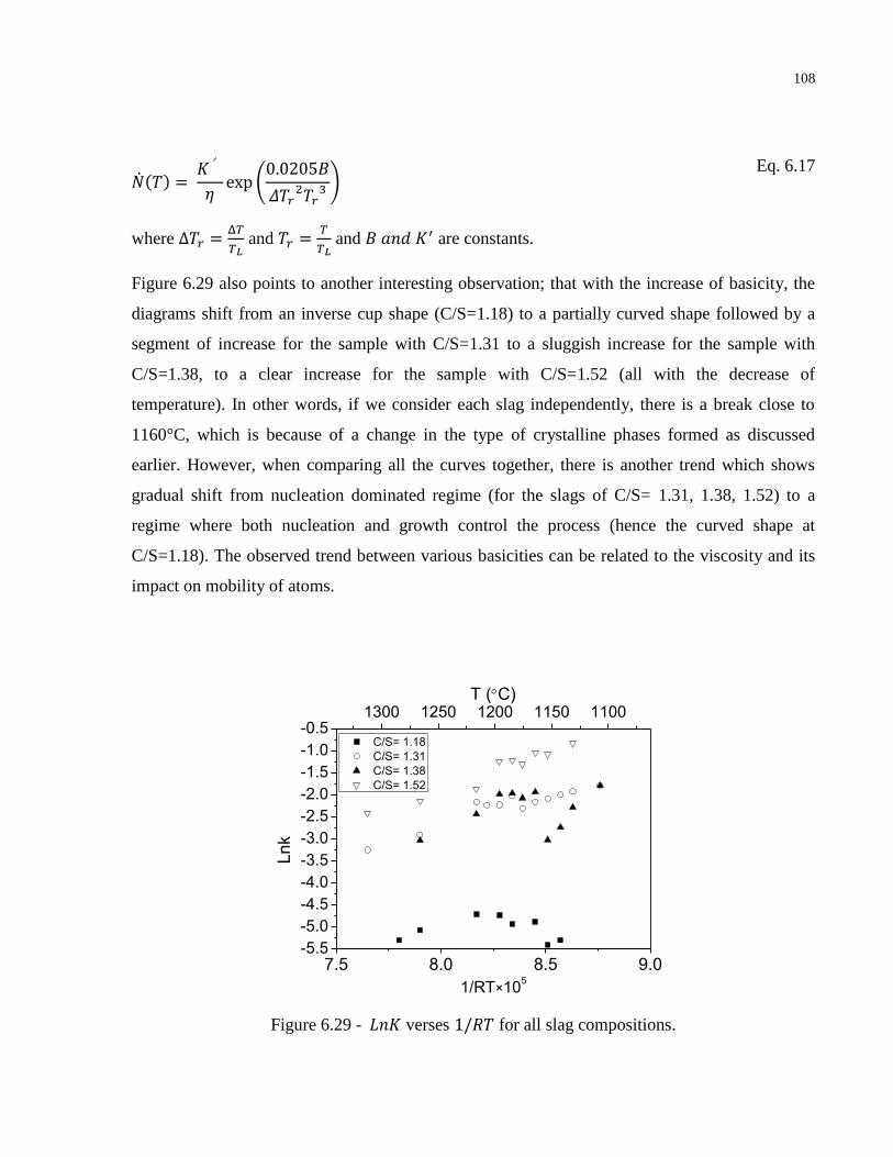
108

��(𝑇) = 𝐾′

𝜂exp (

0.0205𝐵

𝛥𝑇𝑟2𝑇𝑟

3 ) Eq. 6.17

where Δ𝑇𝑟 =Δ𝑇

𝑇𝐿 and 𝑇𝑟 =

𝑇

𝑇𝐿 and 𝐵 𝑎𝑛𝑑 𝐾′ are constants.

Figure 6.29 also points to another interesting observation; that with the increase of basicity, the

diagrams shift from an inverse cup shape (C/S=1.18) to a partially curved shape followed by a

segment of increase for the sample with C/S=1.31 to a sluggish increase for the sample with

C/S=1.38, to a clear increase for the sample with C/S=1.52 (all with the decrease of

temperature). In other words, if we consider each slag independently, there is a break close to

1160°C, which is because of a change in the type of crystalline phases formed as discussed

earlier. However, when comparing all the curves together, there is another trend which shows

gradual shift from nucleation dominated regime (for the slags of C/S= 1.31, 1.38, 1.52) to a

regime where both nucleation and growth control the process (hence the curved shape at

C/S=1.18). The observed trend between various basicities can be related to the viscosity and its

impact on mobility of atoms.

7.5 8.0 8.5 9.0-5.5

-5.0

-4.5

-4.0

-3.5

-3.0

-2.5

-2.0

-1.5

-1.0

-0.5

T (C)

C/S= 1.18

C/S= 1.31

C/S= 1.38

C/S= 1.52

Lnk

1/RT×105

1300 1250 1200 1150 1100

Figure 6.29 - 𝐿𝑛𝐾 verses 1/𝑅𝑇 for all slag compositions.

109

Based on the discussion above, the composite effect of the different dependence of nucleation

and growth on temperature results in the decrease in K with temperature, the way seen in Figure

6.22 – 6.24 and 6.26. In other words, fitting the data to an Arrhenius type correlation yields an

effective activation energy that is only a fitting parameter, and not a true indicator of an intrinsic

energy barrier for phase transformation.

110

Chapter 7

Mathematical modeling of slag crystallization and heat recovery

Two mathematical models were developed and employed in combination with experimental data

to calculate the extent of heat recovery and slag crystallization, two parameters of foremost

importance, in a simplified slag processing unit. The first model was developed to calculate the

temperature history of slag during its cooling to allow optimizing the air/slag ratio for both heat

recovery and slag glass content. This model was later combined with the second which was

aimed to predict the amount of crystallization during cooling. The results were validated by

experiments involving non-isothermal crystallization of slag particles that represent a real slag

cooling scenario.

Modeling the heat recovery process

In the heat recovery model, it is assumed that slag droplets of known size are released into a

vertical heat recovery vessel/duct. While descending, the counter–current air flow cools the

droplets and receives their thermal energy. The purpose of the model is to (a) obtain cooling rate

of slag particles which will be used in the second model to predict glass content, (b) calculate the

amount of heat recovered into hot air, as a function of parameters such as air/slag ratio and slag

granule size.

Assumptions

The key assumptions in the existing code are the following:

1. The heat is transferred from the center of the liquid slag droplet to the slag surface by

conduction and later by convection and radiation to air (Figure 7.1).

2. Air temperature is assumed uniform but the droplets are considered to have a temperature

gradient.

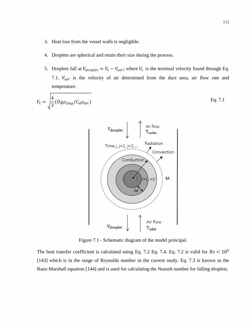
111

3. Heat loss from the vessel walls is negligible.

4. Droplets are spherical and retain their size during the process.

5. Droplets fall at 𝑉𝑑𝑟𝑜𝑝𝑙𝑒𝑡 = 𝑉𝑡 − 𝑉𝑎𝑖𝑟; where 𝑉𝑡 is the terminal velocity found through Eq.

7.1. 𝑉𝑎𝑖𝑟 is the velocity of air determined from the duct area, air flow rate and

temperature.

𝑉𝑡 = √4

3(𝐷𝑔𝜌𝑠𝑙𝑎𝑔/𝐶𝑑𝜌𝑎𝑖𝑟) Eq. 7.1

Figure 7.1 - Schematic diagram of the model principal.

The heat transfer coefficient is calculated using Eq. 7.2 Eq. 7.4. Eq. 7.2 is valid for 𝑅𝑒 < 105

[143] which is in the range of Reynolds number in the current study. Eq. 7.3 is known as the

Ranz-Marshall equation [144] and is used for calculating the Nusselt number for falling droplets.

112

𝑅𝑒 = 𝑉𝑡 × 𝐷 × 𝜌𝑎𝑖𝑟/𝑣𝑎𝑖𝑟 Eq. 7.2

𝑁𝑢 = 2 + 0.6 (𝑅𝑒1 2⁄ × 𝑃𝑟1 3⁄ ) Eq. 7.3

ℎ = 𝑁𝑢 × 𝐾𝐴𝑖𝑟/𝐷 Eq. 7.4

In the above equations, 𝐷 is the droplet diameter, 𝜌𝑎𝑖𝑟, 𝑣𝑎𝑖𝑟 and 𝑃𝑟 are the air density, kinematic

viscosity and Prandtl number respectively.

Enthalpy method

The enthalpy method was adapted for the calculations of phase change and heat transfer in

moving boundary problems especially in situations in which the material does not have a distinct

solid/liquid interface such as glassy substances (Figure 7.2 - a). In such systems, the melting or

solidification takes place over an extended range of temperatures (Figure 7.2 - b) and the solid

and liquid are separated by a two-phase moving region. In this approach, an enthalpy function,

𝐻(𝑇), which represents the total heat content of the substance, is used as a dependant variable,

being a function of temperature for the given material.

The enthalpy formulation of this phase change problem is given by Eq. 7.5 which is considered

valid over the entire solution domain including the solid and liquid phases as well as the

interface.

𝜌𝜕𝐻(𝑇)

𝜕𝑡= ∇. (𝑘∇T)

Eq. 7.5

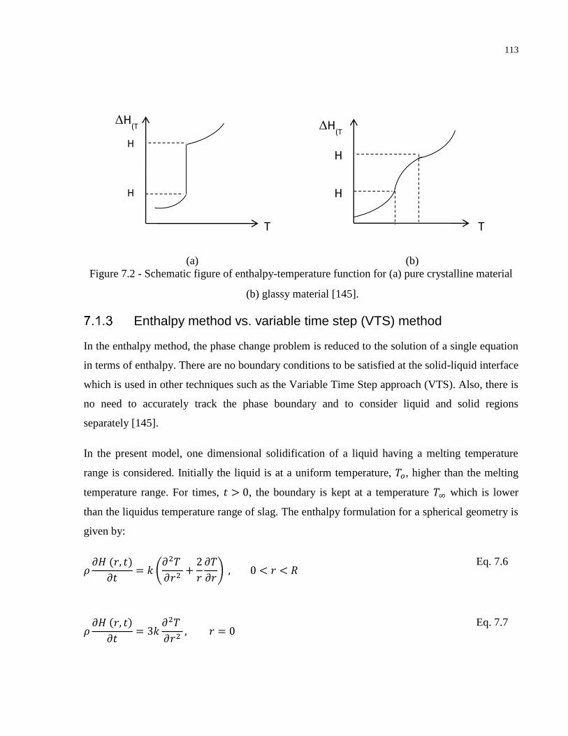
113

(a) (b)

Figure 7.2 - Schematic figure of enthalpy-temperature function for (a) pure crystalline material

(b) glassy material [145].

Enthalpy method vs. variable time step (VTS) method

In the enthalpy method, the phase change problem is reduced to the solution of a single equation

in terms of enthalpy. There are no boundary conditions to be satisfied at the solid-liquid interface

which is used in other techniques such as the Variable Time Step approach (VTS). Also, there is

no need to accurately track the phase boundary and to consider liquid and solid regions

separately [145].

In the present model, one dimensional solidification of a liquid having a melting temperature

range is considered. Initially the liquid is at a uniform temperature, 𝑇𝑜, higher than the melting

temperature range. For times, 𝑡 > 0, the boundary is kept at a temperature 𝑇∞ which is lower

than the liquidus temperature range of slag. The enthalpy formulation for a spherical geometry is

given by:

𝜌𝜕𝐻 (𝑟, 𝑡)

𝜕𝑡= 𝑘 (

𝜕2𝑇

𝜕𝑟2+

2

𝑟

𝜕𝑇

𝜕𝑟) , 0 < 𝑟 < 𝑅

Eq. 7.6

𝜌𝜕𝐻 (𝑟, 𝑡)

𝜕𝑡= 3𝑘

𝜕2𝑇

𝜕𝑟2, 𝑟 = 0

Eq. 7.7

H

s

H

ΔH(T

T

H

H

ΔH(T

T

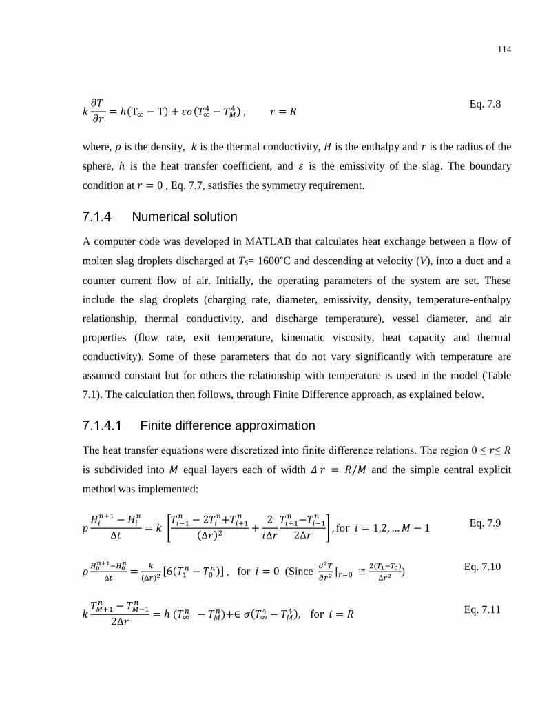
114

𝑘𝜕𝑇

𝜕𝑟= ℎ(T∞ − T) + 𝜀𝜎(𝑇∞

4 − 𝑇𝑀4 ) , 𝑟 = 𝑅

Eq. 7.8

where, 𝜌 is the density, 𝑘 is the thermal conductivity, 𝐻 is the enthalpy and 𝑟 is the radius of the

sphere, ℎ is the heat transfer coefficient, and 𝜀 is the emissivity of the slag. The boundary

condition at 𝑟 = 0 , Eq. 7.7, satisfies the symmetry requirement.

Numerical solution

A computer code was developed in MATLAB that calculates heat exchange between a flow of

molten slag droplets discharged at TS= 1600°C and descending at velocity (V), into a duct and a

counter current flow of air. Initially, the operating parameters of the system are set. These

include the slag droplets (charging rate, diameter, emissivity, density, temperature-enthalpy

relationship, thermal conductivity, and discharge temperature), vessel diameter, and air

properties (flow rate, exit temperature, kinematic viscosity, heat capacity and thermal

conductivity). Some of these parameters that do not vary significantly with temperature are

assumed constant but for others the relationship with temperature is used in the model (Table

7.1). The calculation then follows, through Finite Difference approach, as explained below.

Finite difference approximation

The heat transfer equations were discretized into finite difference relations. The region 0 ≤ 𝑟≤ 𝑅

is subdivided into 𝑀 equal layers each of width 𝛥 𝑟 = 𝑅/𝑀 and the simple central explicit

method was implemented:

𝑝𝐻𝑖

𝑛+1 − 𝐻𝑖𝑛

∆𝑡= 𝑘 [

𝑇𝑖−1𝑛 − 2𝑇𝑖

𝑛+𝑇𝑖+1𝑛

(∆𝑟)2+

2

𝑖∆𝑟

𝑇𝑖+1𝑛 −𝑇𝑖−1

𝑛

2∆𝑟] , for 𝑖 = 1,2, … 𝑀 − 1 Eq. 7.9

𝜌𝐻0

𝑛+1−𝐻0𝑛

∆𝑡=

𝑘

(∆𝑟)2[6(𝑇1

𝑛 − 𝑇0𝑛)] , for 𝑖 = 0 (Since

𝜕2𝑇

𝜕𝑟2|𝑟=0 ≅

2(𝑇1−𝑇0)

∆𝑟2) Eq. 7.10

𝑘𝑇𝑀+1

𝑛 − 𝑇𝑀−1𝑛

2∆𝑟= ℎ (𝑇∞

𝑛 − 𝑇𝑀𝑛)+∈ 𝜎(𝑇∞

4 − 𝑇𝑀4 ), for 𝑖 = 𝑅 Eq. 7.11

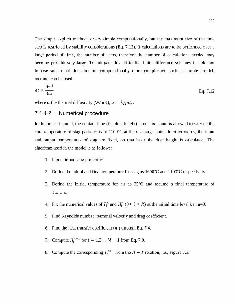
115

The simple explicit method is very simple computationally, but the maximum size of the time

step is restricted by stability considerations (Eq. 7.12). If calculations are to be performed over a

large period of time, the number of steps, therefore the number of calculations needed may

become prohibitively large. To mitigate this difficulty, finite difference schemes that do not

impose such restrictions but are computationally more complicated such as simple implicit

method, can be used.

𝛥𝑡 ≤𝛥𝑟 2

6𝛼 Eq. 7.12

where 𝛼 the thermal diffusivity (W/mK), 𝛼 = 𝑘/𝜌𝐶𝑝.

Numerical procedure

In the present model, the contact time (the duct height) is not fixed and is allowed to vary so the

core temperature of slag particles is at 1100°C at the discharge point. In other words, the input

and output temperatures of slag are fixed, on that basis the duct height is calculated. The

algorithm used in the model is as follows:

1. Input air and slag properties.

2. Define the initial and final temperature for slag as 1600°C and 1100°C respectively.

3. Define the initial temperature for air as 25°C and assume a final temperature of

Tair_outlet.

4. Fix the numerical values of 𝑇𝑖𝑛 and 𝐻𝑖

𝑛 (0≤ 𝑖 ≤ 𝑅) at the initial time level i.e., n=0.

5. Find Reynolds number, terminal velocity and drag coefficient.

6. Find the heat transfer coefficient (ℎ ) through Eq. 7.4.

7. Compute 𝐻𝑖𝑛+1 for 𝑖 = 1,2, … 𝑀 − 1 from Eq. 7.9.

8. Compute the corresponding 𝑇𝑖𝑛+1 from the 𝐻 − 𝑇 relation, i.e., Figure 7.3.

116

9. Determine 𝑇𝑀𝑛+1 for the surface boundary condition at 𝑟 = 𝑅, by finite difference

representation of Eq. 7.11.

By the end of this step, heat transfer by conduction from the slag core to surface at time level

n+1 is completed.

10. Calculate the total heat transferred from the slag droplets to air by convection and

radiation during time interval 𝑛 to 𝑛 + 1 by the heat balance equation and update the air

temperature.

11. Repeat the above steps until the air inlet temperature reaches 25°C.

12. Find the slag core temperature. If the temperature is higher or lower than 1100°C,

increase or decrease the Tair_outlet respectively.

13. Repeat step 1-11 until Tair_outlet results in a slag core temperature of 1100°C.

As a base case, the following parameters were used, and varied when applicable to investigate

the effect of each parameter on the heat transfer efficiency.

1. The target core temperature of 1100°C temperature is based on the slag clustering

temperature. As explained in Chapter 2, in a two-step heat recovery process which is

considered the most efficient method for heat recovery [29], the slag granules are

discharged from a fluidized bed to a packed bed after reaching the clustering

temperature which is typically 900 °C-1100°C. When the slag reaches 900°C on the

surface, the core temperature will be about 1100°C. This would ensure the slag granules

will not stick to each other. Another reason for choosing 1100°C as the target

temperature is that it is close to the nose temperature of a typical BF slag time‒

temperature–transformation (TTT) diagram which is the temperature that the slag

experiences the highest crystallization rate. In other words, if the core reaches this

temperature and does not crystalize we can be certain that it will not crystallize after

this point in any of the other layers.

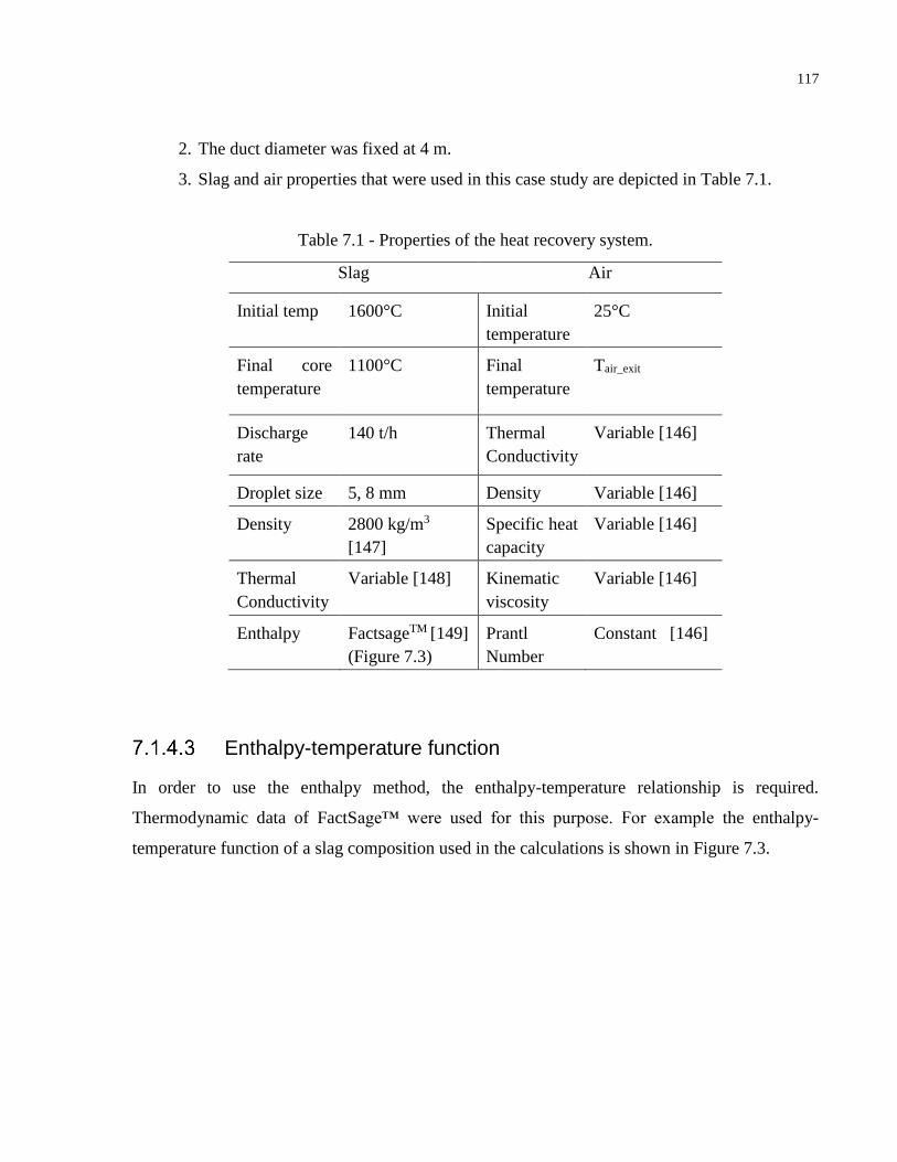
117

2. The duct diameter was fixed at 4 m.

3. Slag and air properties that were used in this case study are depicted in Table 7.1.

Table 7.1 - Properties of the heat recovery system.

Slag Air

Initial temp 1600°C Initial

temperature

25°C

Final core

temperature

1100°C Final

temperature

Tair_exit

Discharge

rate

140 t/h Thermal

Conductivity

Variable [146]

Droplet size 5, 8 mm Density Variable [146]

Density 2800 kg/m3

[147]

Specific heat

capacity

Variable [146]

Thermal

Conductivity

Variable [148] Kinematic

viscosity

Variable [146]

Enthalpy FactsageTM [149]

(Figure 7.3)

Prantl

Number

Constant [146]

Enthalpy-temperature function

In order to use the enthalpy method, the enthalpy-temperature relationship is required.

Thermodynamic data of FactSage™ were used for this purpose. For example the enthalpy-

temperature function of a slag composition used in the calculations is shown in Figure 7.3.

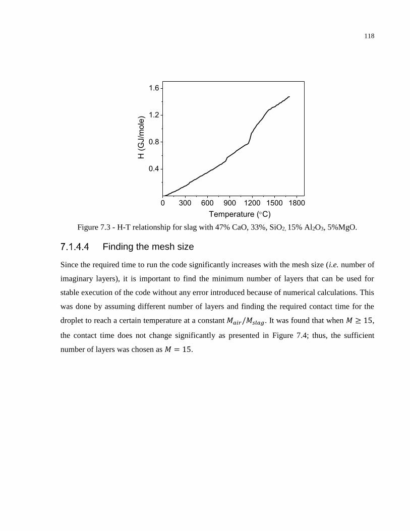
118

0 300 600 900 1200 1500 1800

0.4

0.8

1.2

1.6

H (

GJ/m

ole

)

Temperature (C)

Figure 7.3 - H-T relationship for slag with 47% CaO, 33%, SiO2, 15% Al2O3, 5%MgO.

Finding the mesh size

Since the required time to run the code significantly increases with the mesh size (i.e. number of

imaginary layers), it is important to find the minimum number of layers that can be used for

stable execution of the code without any error introduced because of numerical calculations. This

was done by assuming different number of layers and finding the required contact time for the

droplet to reach a certain temperature at a constant 𝑀𝑎𝑖𝑟/𝑀𝑠𝑙𝑎𝑔. It was found that when 𝑀 ≥ 15,

the contact time does not change significantly as presented in Figure 7.4; thus, the sufficient

number of layers was chosen as 𝑀 = 15.

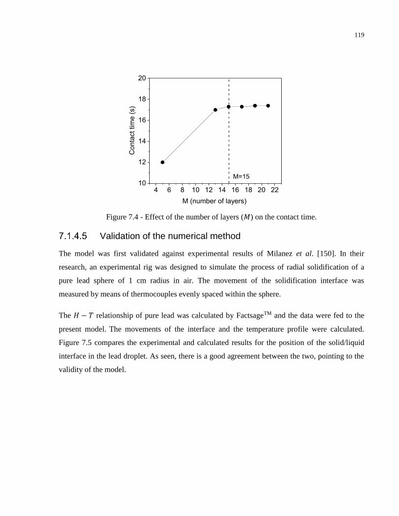
119

4 6 8 10 12 14 16 18 20 2210

12

14

16

18

20

Conta

ct tim

e (

s)

M (number of layers)

M=15

Figure 7.4 - Effect of the number of layers (𝑀) on the contact time.

Validation of the numerical method

The model was first validated against experimental results of Milanez et al. [150]. In their

research, an experimental rig was designed to simulate the process of radial solidification of a

pure lead sphere of 1 cm radius in air. The movement of the solidification interface was

measured by means of thermocouples evenly spaced within the sphere.

The 𝐻 − 𝑇 relationship of pure lead was calculated by FactsageTM and the data were fed to the

present model. The movements of the interface and the temperature profile were calculated.

Figure 7.5 compares the experimental and calculated results for the position of the solid/liquid

interface in the lead droplet. As seen, there is a good agreement between the two, pointing to the

validity of the model.

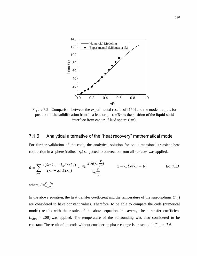
120

0.0 0.2 0.4 0.6 0.8 1.00

20

40

60

80

100

120

140

Numercial Modeling

Experimental (Milanez et al.)

Tim

e (

s)

r/R

Figure 7.5 - Comparison between the experimental results of [150] and the model outputs for

position of the solidification front in a lead droplet. r/R= is the position of the liquid-solid

interface from center of lead sphere (cm).

Analytical alternative of the “heat recovery” mathematical model

For further validation of the code, the analytical solution for one-dimensional transient heat

conduction in a sphere (radius= 𝑟0) subjected to convection from all surfaces was applied.

𝜃 = ∑4(𝑆𝑖𝑛𝜆𝑛 − 𝜆𝑛𝐶𝑜𝑠𝜆𝑛)

2𝜆𝑛 − 𝑆𝑖𝑛(2𝜆𝑛)

∞

𝑛=1

𝑒−𝜆𝑛2 Ƭ

𝑆𝑖𝑛(𝜆𝑛𝑟𝑟0

)

𝜆𝑛𝑟𝑟0

1 − 𝜆𝑛𝐶𝑜𝑡𝜆𝑛 = 𝐵𝑖 Eq. 7.13

where, 𝜃=𝑇𝑖−𝑇∞

𝑇−𝑇∞.

In the above equation, the heat transfer coefficient and the temperature of the surroundings (𝑇∞)

are considered to have constant values. Therefore, to be able to compare the code (numerical

model) results with the results of the above equation, the average heat transfer coefficient

(ℎ𝐴𝑣𝑔 = 200) was applied. The temperature of the surrounding was also considered to be

constant. The result of the code without considering phase change is presented in Figure 7.6.

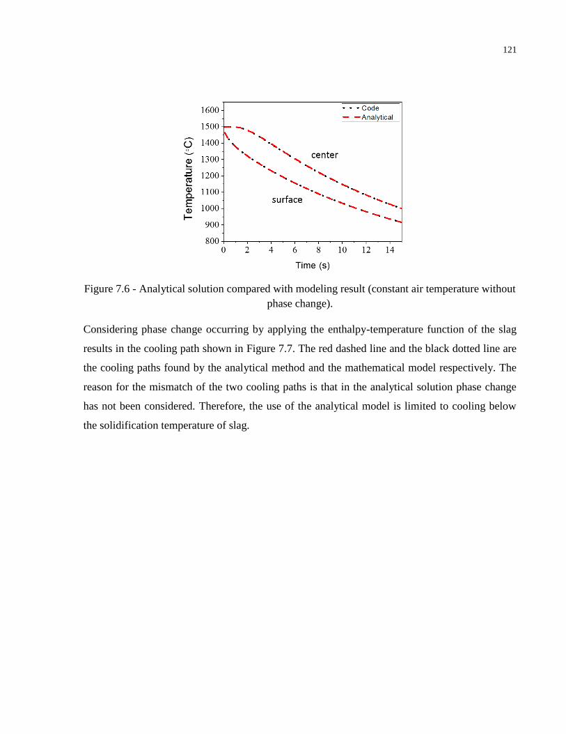
121

Figure 7.6 - Analytical solution compared with modeling result (constant air temperature without

phase change).

Considering phase change occurring by applying the enthalpy-temperature function of the slag

results in the cooling path shown in Figure 7.7. The red dashed line and the black dotted line are

the cooling paths found by the analytical method and the mathematical model respectively. The

reason for the mismatch of the two cooling paths is that in the analytical solution phase change

has not been considered. Therefore, the use of the analytical model is limited to cooling below

the solidification temperature of slag.

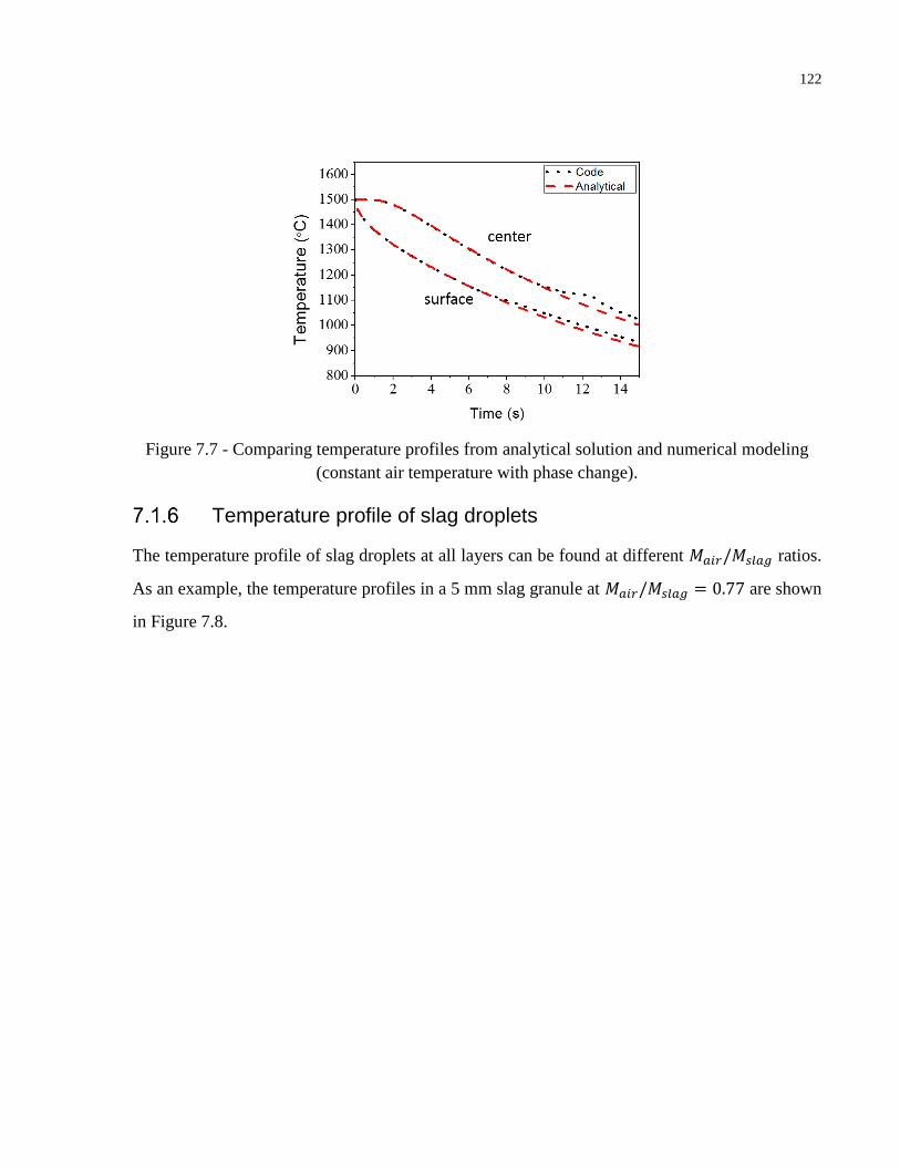
122

Figure 7.7 - Comparing temperature profiles from analytical solution and numerical modeling

(constant air temperature with phase change).

Temperature profile of slag droplets

The temperature profile of slag droplets at all layers can be found at different 𝑀𝑎𝑖𝑟/𝑀𝑠𝑙𝑎𝑔 ratios.

As an example, the temperature profiles in a 5 mm slag granule at 𝑀𝑎𝑖𝑟/𝑀𝑠𝑙𝑎𝑔 = 0.77 are shown

in Figure 7.8.

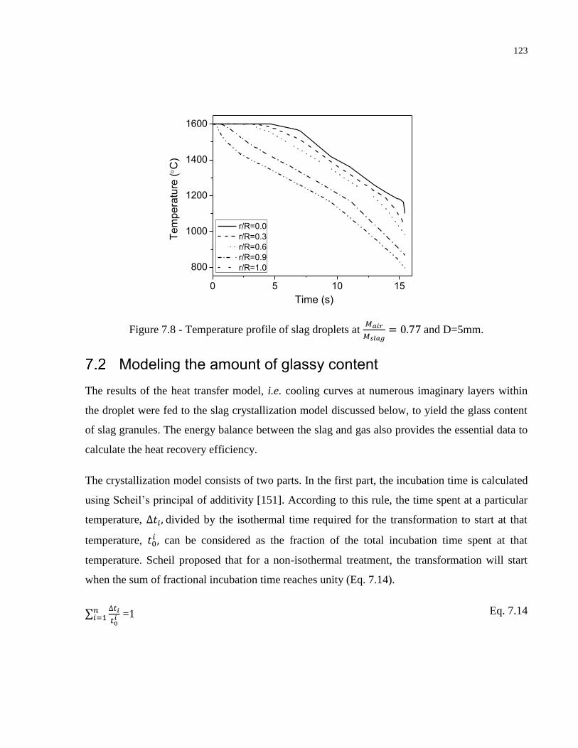
123

0 5 10 15

800

1000

1200

1400

1600

Tem

pe

ratu

re (C

)

Time (s)

r/R=0.0

r/R=0.3

r/R=0.6

r/R=0.9

r/R=1.0

Figure 7.8 - Temperature profile of slag droplets at 𝑀𝑎𝑖𝑟

𝑀𝑠𝑙𝑎𝑔= 0.77 and D=5mm.

Modeling the amount of glassy content

The results of the heat transfer model, i.e. cooling curves at numerous imaginary layers within

the droplet were fed to the slag crystallization model discussed below, to yield the glass content

of slag granules. The energy balance between the slag and gas also provides the essential data to

calculate the heat recovery efficiency.

The crystallization model consists of two parts. In the first part, the incubation time is calculated

using Scheil’s principal of additivity [151]. According to this rule, the time spent at a particular

temperature, ∆𝑡𝑖, divided by the isothermal time required for the transformation to start at that

temperature, 𝑡0𝑖 , can be considered as the fraction of the total incubation time spent at that

temperature. Scheil proposed that for a non-isothermal treatment, the transformation will start

when the sum of fractional incubation time reaches unity (Eq. 7.14).

∑∆𝑡𝑖

𝑡0𝑖

𝑛𝑖=1 =1 Eq. 7.14

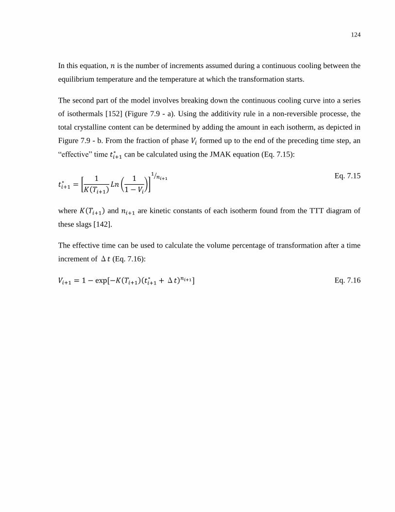
124

In this equation, 𝑛 is the number of increments assumed during a continuous cooling between the

equilibrium temperature and the temperature at which the transformation starts.

The second part of the model involves breaking down the continuous cooling curve into a series

of isothermals [152] (Figure 7.9 - a). Using the additivity rule in a non-reversible processe, the

total crystalline content can be determined by adding the amount in each isotherm, as depicted in

Figure 7.9 - b. From the fraction of phase 𝑉𝑖 formed up to the end of the preceding time step, an

“effective” time 𝑡𝑖+1∗ can be calculated using the JMAK equation (Eq. 7.15):

𝑡𝑖+1∗ = [

1

𝐾(𝑇𝑖+1)𝐿𝑛 (

1

1 − 𝑉𝑖)]

1𝑛𝑖+1

⁄

Eq. 7.15

where 𝐾(𝑇𝑖+1) and 𝑛𝑖+1 are kinetic constants of each isotherm found from the TTT diagram of

these slags [142].

The effective time can be used to calculate the volume percentage of transformation after a time

increment of Δ𝑡 (Eq. 7.16):

𝑉𝑖+1 = 1 − exp [−𝐾(𝑇𝑖+1)(𝑡𝑖+1∗ +Δ𝑡)𝑛𝑖+1] Eq. 7.16

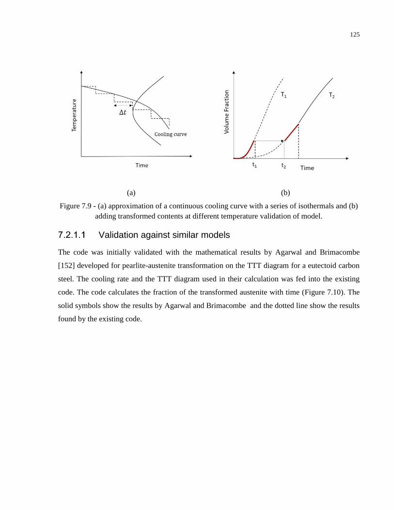
125

(a) (b)

Figure 7.9 - (a) approximation of a continuous cooling curve with a series of isothermals and (b)

adding transformed contents at different temperature validation of model.

Validation against similar models

The code was initially validated with the mathematical results by Agarwal and Brimacombe

[152] developed for pearlite-austenite transformation on the TTT diagram for a eutectoid carbon

steel. The cooling rate and the TTT diagram used in their calculation was fed into the existing

code. The code calculates the fraction of the transformed austenite with time (Figure 7.10). The

solid symbols show the results by Agarwal and Brimacombe and the dotted line show the results

found by the existing code.

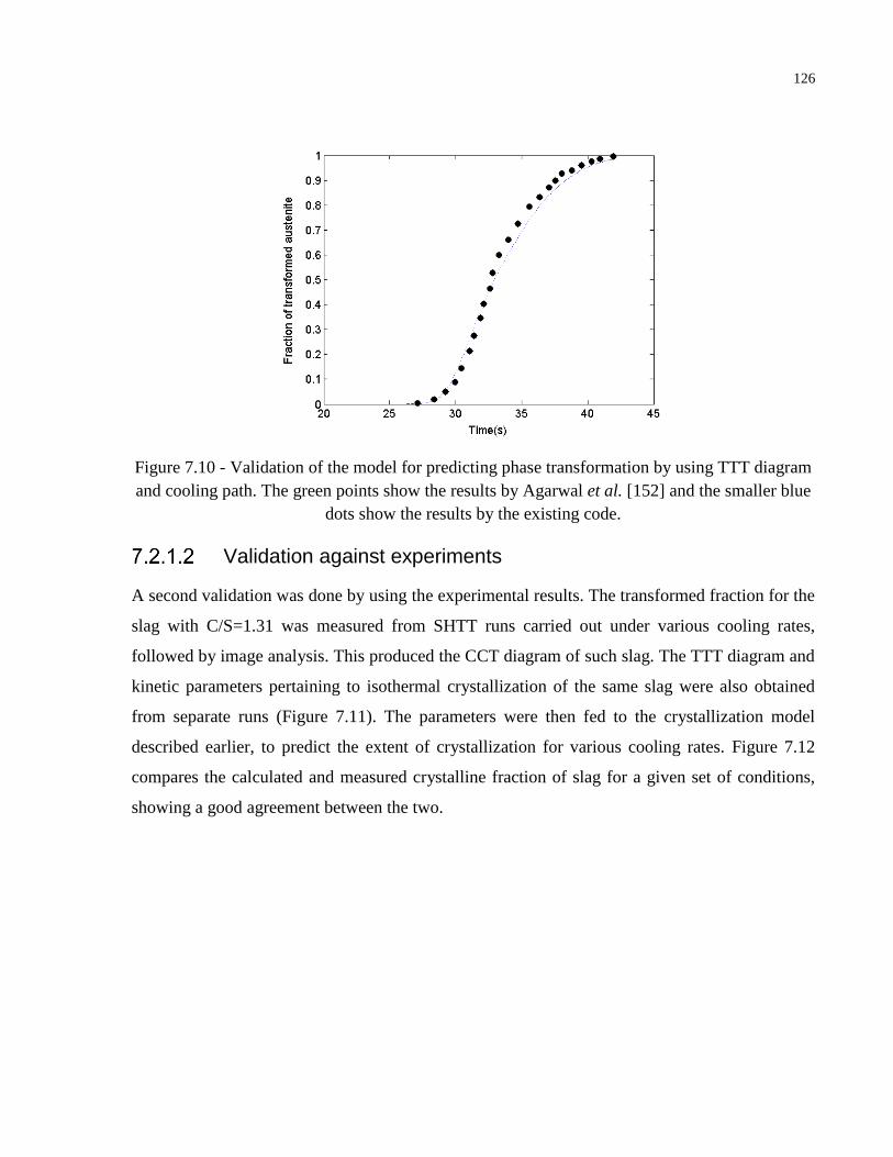
126

Figure 7.10 - Validation of the model for predicting phase transformation by using TTT diagram

and cooling path. The green points show the results by Agarwal et al. [152] and the smaller blue

dots show the results by the existing code.

Validation against experiments

A second validation was done by using the experimental results. The transformed fraction for the

slag with C/S=1.31 was measured from SHTT runs carried out under various cooling rates,

followed by image analysis. This produced the CCT diagram of such slag. The TTT diagram and

kinetic parameters pertaining to isothermal crystallization of the same slag were also obtained

from separate runs (Figure 7.11). The parameters were then fed to the crystallization model

described earlier, to predict the extent of crystallization for various cooling rates. Figure 7.12

compares the calculated and measured crystalline fraction of slag for a given set of conditions,

showing a good agreement between the two.

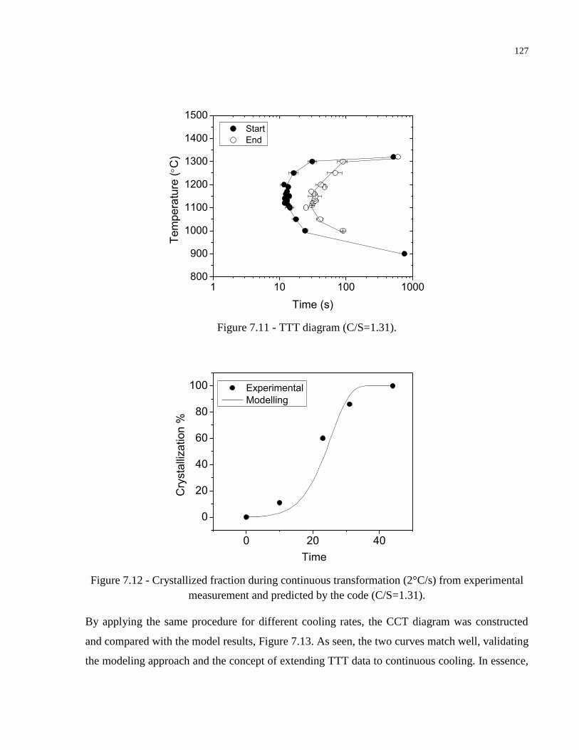
127

1 10 100 1000800

900

1000

1100

1200

1300

1400

1500

Start

End

Tem

pera

ture

(C

)

Time (s)

Figure 7.11 - TTT diagram (C/S=1.31).

0 20 40

0

20

40

60

80

100

Experimental

Modelling

Cry

sta

llization %

Time

Figure 7.12 - Crystallized fraction during continuous transformation (2°C/s) from experimental

measurement and predicted by the code (C/S=1.31).

By applying the same procedure for different cooling rates, the CCT diagram was constructed

and compared with the model results, Figure 7.13. As seen, the two curves match well, validating

the modeling approach and the concept of extending TTT data to continuous cooling. In essence,

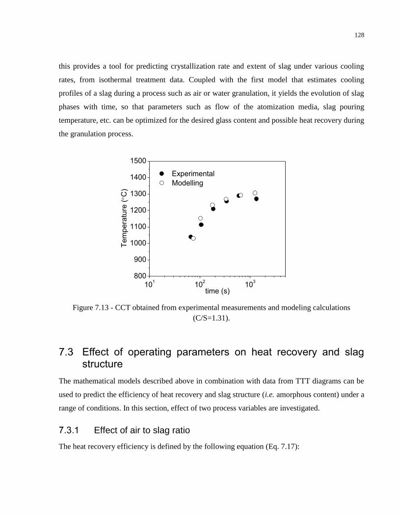
128

this provides a tool for predicting crystallization rate and extent of slag under various cooling

rates, from isothermal treatment data. Coupled with the first model that estimates cooling

profiles of a slag during a process such as air or water granulation, it yields the evolution of slag

phases with time, so that parameters such as flow of the atomization media, slag pouring

temperature, etc. can be optimized for the desired glass content and possible heat recovery during

the granulation process.

Figure 7.13 - CCT obtained from experimental measurements and modeling calculations

(C/S=1.31).

Effect of operating parameters on heat recovery and slag structure

The mathematical models described above in combination with data from TTT diagrams can be

used to predict the efficiency of heat recovery and slag structure (i.e. amorphous content) under a

range of conditions. In this section, effect of two process variables are investigated.

Effect of air to slag ratio

The heat recovery efficiency is defined by the following equation (Eq. 7.17):

101

102

103

800

900

1000

1100

1200

1300

1400

1500

Experimental

Modelling

Tem

pera

ture

(C

)

time (s)

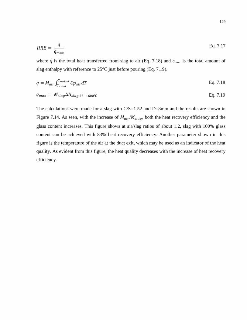
129

𝐻𝑅𝐸 = 𝑞

𝑞𝑚𝑎𝑥 Eq. 7.17

where q is the total heat transferred from slag to air (Eq. 7.18) and 𝑞𝑚𝑎𝑥 is the total amount of

slag enthalpy with reference to 25°C just before pouring (Eq. 7.19).

𝑞 = 𝑀𝑎𝑖𝑟 ∫ 𝐶𝑝𝑎𝑖𝑟𝑑𝑇𝑇𝑜𝑢𝑡𝑙𝑒𝑡

𝑇𝑖𝑛𝑙𝑒𝑡 Eq. 7.18

𝑞𝑚𝑎𝑥 = 𝑀𝑠𝑙𝑎𝑔∆𝐻𝑠𝑙𝑎𝑔,25−1600℃ Eq. 7.19

The calculations were made for a slag with C/S=1.52 and D=8mm and the results are shown in

Figure 7.14. As seen, with the increase of 𝑀𝑎𝑖𝑟/𝑀𝑠𝑙𝑎𝑔, both the heat recovery efficiency and the

glass content increases. This figure shows at air/slag ratios of about 1.2, slag with 100% glass

content can be achieved with 83% heat recovery efficiency. Another parameter shown in this

figure is the temperature of the air at the duct exit, which may be used as an indicator of the heat

quality. As evident from this figure, the heat quality decreases with the increase of heat recovery

efficiency.

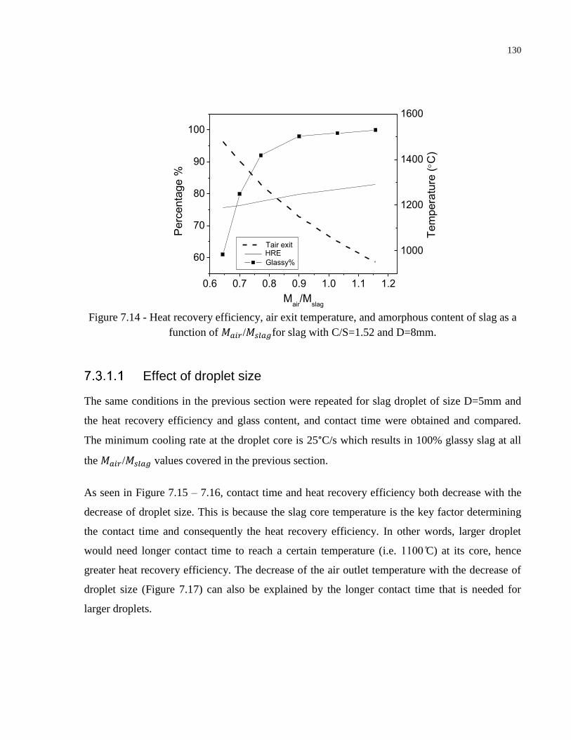
130

0.6 0.7 0.8 0.9 1.0 1.1 1.2

60

70

80

90

100

Tem

pera

ture

(C

)

Perc

enta

ge %

Mair

/Mslag

HRE

Glassy%

1000

1200

1400

1600

Tair exit

Figure 7.14 - Heat recovery efficiency, air exit temperature, and amorphous content of slag as a

function of 𝑀𝑎𝑖𝑟/𝑀𝑠𝑙𝑎𝑔for slag with C/S=1.52 and D=8mm.

Effect of droplet size

The same conditions in the previous section were repeated for slag droplet of size D=5mm and

the heat recovery efficiency and glass content, and contact time were obtained and compared.

The minimum cooling rate at the droplet core is 25°C/s which results in 100% glassy slag at all

the 𝑀𝑎𝑖𝑟/𝑀𝑠𝑙𝑎𝑔 values covered in the previous section.

As seen in Figure 7.15 – 7.16, contact time and heat recovery efficiency both decrease with the

decrease of droplet size. This is because the slag core temperature is the key factor determining

the contact time and consequently the heat recovery efficiency. In other words, larger droplet

would need longer contact time to reach a certain temperature (i.e. 1100 C) at its core, hence

greater heat recovery efficiency. The decrease of the air outlet temperature with the decrease of

droplet size (Figure 7.17) can also be explained by the longer contact time that is needed for

larger droplets.

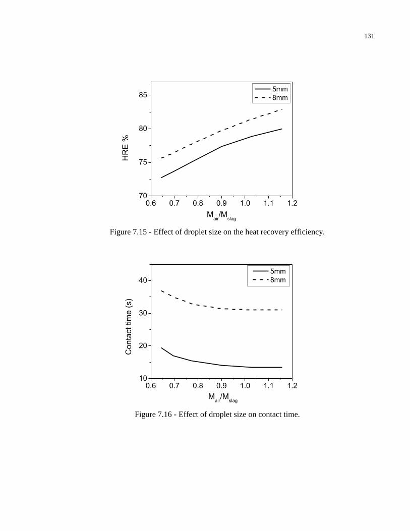
131

0.6 0.7 0.8 0.9 1.0 1.1 1.270

75

80

85

HR

E %

Mair

/Mslag

5mm

8mm

Figure 7.15 - Effect of droplet size on the heat recovery efficiency.

0.6 0.7 0.8 0.9 1.0 1.1 1.210

20

30

40

Conta

ct tim

e (

s)

Mair

/Mslag

5mm

8mm

Figure 7.16 - Effect of droplet size on contact time.

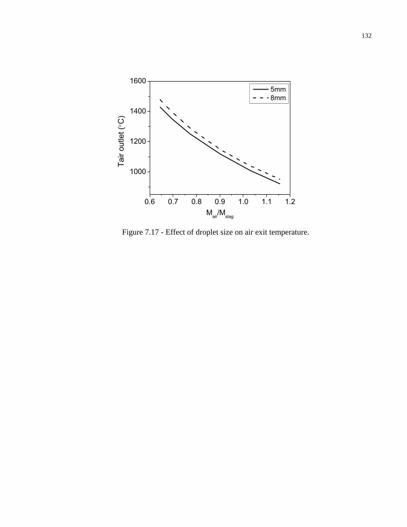
132

0.6 0.7 0.8 0.9 1.0 1.1 1.2

1000

1200

1400

1600

Tair o

utlet (

C)

Mair

/Mslag

5mm

8mm

Figure 7.17 - Effect of droplet size on air exit temperature.

133

Chapter 8

Contributions and conclusions

Conclusions

The main conclusions of this work can be summarized in three sections:

A) Simultaneous temperature measurement and in-situ observation of slag in a SHTT device

allowed derivation of TTT and CCT diagrams for several slags with NBO/T ratios in the range of

0.77 to 1.94. It was found that:

1. With an increase in basicity, the TTT and CCT diagrams of glassy to crystalline

transformation shift to the left (shorter time) and to higher temperatures.

2. The dependence of slag crystallization behavior on the slag composition changes at

NBO/T 1.6. Crystallization features at higher basicity are faster crystallization and

opaque crystalline phases, whereas for lower basicity the crystals are translucent.

3. For slags with NBO/T 1.6, equiaxed crystals are formed at high temperatures. As the

temperature drops, first planar, and then again fine equiaxed crystals become the

predominant morphology.

4. For slags with NBO/T<1.6, crystallization involves the growth of very few crystals that

grow to complete the process.

5. The cR values obtained from CCT diagrams are lower than those from TTT diagrams

which agrees with the fact that TTT diagrams present an overestimation of transformation

rate when slag is cooled continuously.

6. The correlation between the optical basicity (Λ𝑐𝑜𝑟𝑟) and cR is stronger than NBO/T with

cR . This is mainly because corrected optical basicity differentiates between the charge-

balancing cations and therefore using this parameter is highly suggested when comparing

the critical cooling rate for different slag compositions especially when the alumina

content changes significantly.

7. The critical cooling rate is inversely proportional to the viscosity.

134

8. A correlation was developed based on theories of nucleation and growth during slag

crystallization to allow prediction of the critical cooling rate using only two parameters:

liquidus temperature ( )LT and viscosity at nose temperature ( nose ) :

𝑅𝑐 = (1.23 × 10−5) (𝑇𝐿2/𝜂𝑛𝑜𝑠𝑒)

B) The transformation kinetics of four slags with varying C/S values were studied using SHTT.

Through image analysis of the samples it was found that the transformation of all samples

followed a sigmoidal form and obeyed the JMAK equation.

1. The Avrami exponent was found and compared with the direct observation during

transformation for four slag compositions. Due to the higher value of 𝑛 (=3-4) for the

slag with C/S=1.52, it was concluded that the crystallization of this sample is diffusion-

controlled growth with increasing nucleation rate. For the samples with C/S=1.31 and

1.38 with n=1.5-2, the growth is controlled by diffusion but the nucleation rate is

decreasing with time. For the slag with the lowest basicity (i.e. C/S=1.18), the n value is

2 at higher temperatures which translates to zero nucleation rate.

2. The mechanism of the growth was found to be diffusion-controlled for all the samples

although the growth has a linear dependence with time. This is in accordance with the

crystals having a dendritic morphology rather than faceted.

3. The overall rate coefficient (K) has the highest value for C/S=1.52 and the smallest for

C/S=1.18. This indicates that the combination of nucleation and growth leads to faster

transformation at higher basicity.

C) A mathematical model was developed to find the effect of droplet size and slag to air ratio on

the required height of a duct in a counter-current heat recovery process. By using the model the

temperature profile of the slag droplets, temperature profile of the air and the cooling rate of the

slag droplets were calculated. The effects of the slag droplet size and slag to air ratio on the slag

exit temperature, the heat recovery efficiency and the height required were investigated.

135

This model also leads to design of the duct (diameter and height) so that the desired slag

discharge temperature at core, e.g. 1100°C, is reached. The contact time can be used as a

reference to predict the required the duct height.

Contributions

This is the most comprehensive research conducted on crystallization behavior of metallurgical

slags to date. Each year more than 650 Mt of slag is produced worldwide containing over 282

TWh worth of energy. This energy is not recovered, as the slag is tapped and cooled slowly in

the slag dumps or is rapidly quenched by water to make amorphous granules that are used as

feedstock for cement manufacturing. The original goal of the study was to investigate the

possibility of recovering the energy from molten slags, while controlling the slag structure so

that it can be used as valuable product.

As the first part of this research, an extensive literature review was conducted which resulted in a

review paper [153] published in the journal Energy and became the “most read article in press”

in the year 2011. Later, experimental and modeling work was performed with focus on the

crystallization behavior of blast furnace slags which is of great interest for generating value-

added products from slag, such as cement feedstock. The main contributions can be explained in

three main sections which is discussed briefly in the following paragraphs.

From practical point of view, this study provided a large set of data on the CCR of slag which

allows a slag processor to determine the proper conditions for obtaining amorphous slag. Further,

a semi-empirical model was developed that enables us to calculate the CCR for a slag, without a

need to do any experiment. This again is a valuable tool for predicting optimum cooling

conditions of slag in an industrial setting.

From scientific point of view, for the first time we have established quantitative and consistent

relationships between crystallization parameters of slag and its chemical composition. The

mechanism and rate of crystallization and their dependence on the composition and temperature

were established. Further, mathematical models were developed and validated that enable

calculations of the most important parameters of a heat recovery process (heat recovery

136

efficiency, amorphous content of slag, and heat quality) as a function of variables such as slag

granule size, air/slag ratio, chamber dimensions, etc. Last, but not least, the HTT method used in

crystallization studies was improved by a new design that is more accurate and easier to set up.

Publications

From this Ph.D. work, 6 journal manuscripts have been submitted or are in preparation which are

presented below.

Journal articles:

1. M. Barati, S. Esfahani, and T. Utigard, "Energy Recovery from High Temperature

Slags," Energy, vol. 36, pp. 5440-5449, 2011.

2. S. Esfahani, Mansoor Barati, "Effect of Slag Composition on the Crystallization of

Synthetic CaO-SiO2-Al2O3-MgO Slags: Part I: Crystallization Behaviour," in press,

Journal of Non-Crystalline Solids.

3. S. Esfahani, Sina Mostaghel, Mansoor Barati, "Effect of Slag Composition on the

Crystallization of Synthetic CaO-SiO2-Al2O3-MgO Slags: Part II- Measurement and

Prediction of Critical Cooling Rate," in press, Journal of Non-Crystalline Solids.

4. S. Esfahani, Karim Danaei, Daniel Budrea, Mansoor Barati, "A Modified Hot

Thermocouple Apparatus for Study of Molten Oxide Solidification and Crystallization,"

accpeted in Measurement Science and Technology

5. S. Esfahani, Mansoor Barati, "Kinetics of Phase Transformation in Synthetic Blast

Furnace Slags” submitted to Journal of Applied Thermal Engineering.

6. S. Esfahani, M. Barati, “Modeling slag crystallization of Blast Furance Slags Pertaining

to Heat Recovery,” to be submitted to Materials Transactions B.

Conference articles:

137

1. S. Esfahani, M. Barati, “Crystallization kinetics of CaO-SiO2-Al2O3-MgO slags,” , to be

submitted to the Sympsium of Moltan Slags, Fluxes and Salts, Seattle 2016

2. S. Esfahani and M. Barati, “Modeling Of Energy Recovery and Slag Structure during

Cooling of Blast Furnace Slags”, in proceedings of COM2015 – 54th Annual Conference

of Metallurgists, Toronto, August 23– 26 2015, Metallurgical Society of CIM, ISBN 978-

1-926872-32-2, 10 pages [Invited]

3. M. Barati and S. Esfahani, “Slag Crystallization Behavior Pertaining to Heat Recovery”,

in Proc. 6th International Congress on the Science and Technology of Steelmaking

(ICS2015), May 12-14, 2015. Beijing, China: Chinese Society of Metals, pp. 889–894

(Keynote Lecture)

4. S. Esfahani, K. Danaei, M. Barati, “Effect of Basicity on the Crystallization Behavior of

Synthetic Slags”, in Proc. Conference of Metallurgists (ISBN: 978-1-926872-24-7), CIM,

2014, 9 pages.

5. S. Esfahani, Y. Kuwauchi, and M. Barati, “A Mathematical Model for Direct Thermal

Heat Recovery From Metallurgical Slags”, in Towards Clean Metallurgical Processing

for Profit and Socio-environmental Stewardship – 51st Conference of Metallurgists,

October 2012, Niagara Falls, Canada, MetSoc–CIM, pp. 183–193

6. S. Esfahani and M. Barati, “Current Status of Heat Recovery from Granulated Slag”, in

3rd International Symposium on High Temperature Metallurgical Processing (TMS

Annual Meeting), Jiang T. et al., eds., Orlando, USA, 2012, TMS, pp. 339–348.

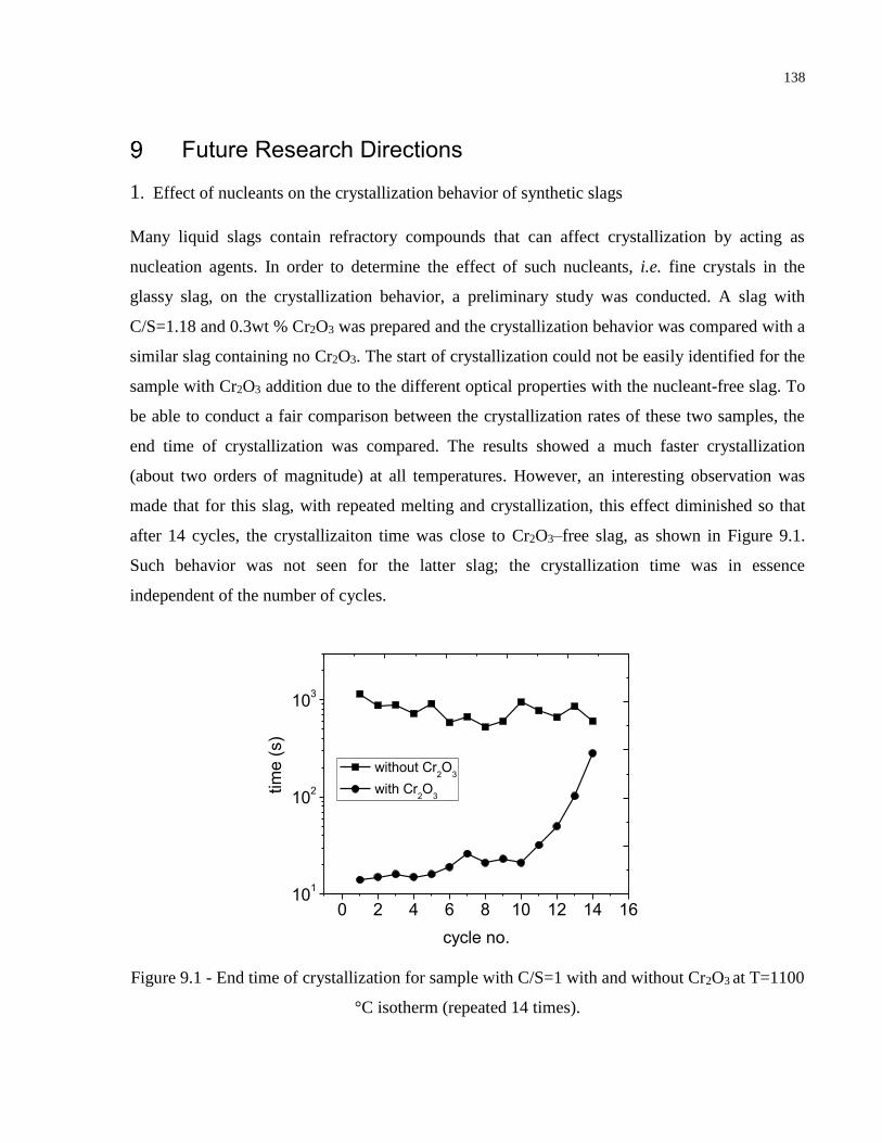
138

Future Research Directions

1. Effect of nucleants on the crystallization behavior of synthetic slags

Many liquid slags contain refractory compounds that can affect crystallization by acting as

nucleation agents. In order to determine the effect of such nucleants, i.e. fine crystals in the

glassy slag, on the crystallization behavior, a preliminary study was conducted. A slag with

C/S=1.18 and 0.3wt % Cr2O3 was prepared and the crystallization behavior was compared with a

similar slag containing no Cr2O3. The start of crystallization could not be easily identified for the

sample with Cr2O3 addition due to the different optical properties with the nucleant-free slag. To

be able to conduct a fair comparison between the crystallization rates of these two samples, the

end time of crystallization was compared. The results showed a much faster crystallization

(about two orders of magnitude) at all temperatures. However, an interesting observation was

made that for this slag, with repeated melting and crystallization, this effect diminished so that

after 14 cycles, the crystallizaiton time was close to Cr2O3–free slag, as shown in Figure 9.1.

Such behavior was not seen for the latter slag; the crystallization time was in essence

independent of the number of cycles.

0 2 4 6 8 10 12 14 1610

1

102

103

tim

e (

s)

cycle no.

without Cr2O

3

with Cr2O

3

Figure 9.1 - End time of crystallization for sample with C/S=1 with and without Cr2O3 at T=1100

°C isotherm (repeated 14 times).

139

Based on this finding, two hypotheses were put forward (1) Cr2O3 containing crystals act as a

nucleant in the first few cycles but later it dissolves in the slag and therefore the crystallization

occurs much slower, or (2) Cr2O3 or Cr2O3 spinel particles agglomerate (or dissolve and

precipitate as larger particles) during each melting-cooling cycle, leading to fewer particles (i.e.

fewer nucleation sites). As the industrial slags often contain such refractory compounds that

would influence crystallization, better understanding of the extent and mechanism of such

nucleation agents is desired.

2. Sintering properties of slag particles

As discussed in Chapter 2 of this thesis, a promising heat recovery system would consist of two

steps, a fluid bed type vessel and a packed bed. The optimum discharge temperature of slag from

the first heat recovery unit to the second would depend on the sintering (sticking) temperature of

the slag particles, as such clustering of particles should be avoided in the packed bed. Although

some have suggested temperatures in the range of 800-1100°C, there is no scientific study to

verify this. Therefore, it is recommended that a study be carried out to develop test procedures

and measure sintering properties of slag as a function of composition. Also, it would be

anticipated that there might be relationships between the sintering temperature and melting or

nose temperature of slag, which can be explored.

140

Bibliography

[1] J. R. Stubbles, "Carbon dioxide emissions from the U.S. steel industry," presented at the

Conference of Metallurgists, Greenhouse Gases in the Metallurgical Industries: Policies,

Abatement and Treatment, Toronto, Canada, 2001.

[2] R. J. Fruehan, O. Fortini, H. W. Paxton, and R. Brindle, "Theoretical minimum energies

to produce steel for selected conditions " U.S. Department of Energy, Washington DC.

2000.

[3] M. Barati and S. Esfahani, "Slag crystallization behavior pertaining to heat recovery," in

The 6th International Congress on the Science and Technology of Steelmaking, Beijing,

China, 2015.

[4] S. K. Biswas, Principles of Blast Furnace Ironmaking. Brisbane, Australia: Cootha

Publishing House, 1981.

[5] L. A. Smirnov and M. I. Panfilov, "Metallurgical slags: properties and application,"

Canadian Metallurgical Quarterly, vol. 32, pp. 173-177, 1988.

[6] M. Barati and K. S. Coley, "Electrical and electronic conductivity of CaO-SiO2-FeOx

slags at various oxygen potentials: Part II. Mechanism and a model of electronic

conduction," Metallurgical and Materials Transactions B-Process Metallurgy and

Materials Processing Science, vol. 37, pp. 51-60, Feb 2006.

[7] M. Allibert, Slag Atlas. Germany: Verlag Stahleisen, 1995.

[8] M. Yoshinaga, K. Fujii, T. Shigematsu, and T. Nakata, "Dry granulation and

solidification of molten blast furnace slag " Transactions of the Iron and Steel Institute of

Japan, vol. 22, pp. 823-829, 1982.

[9] M. P. Sudbury and D. J. Kemp, "The properties and uses of granulated non ferrous

slags," in 2006 TMS Annual Meeting, March 12, 2006 - March 16, 2006, San Antonio,

TX, United states, 2006, pp. 611-620.

[10] J. Nell, 2004, "Melting of platinum group metal concentrates in South Africa," The South

African institute of Mining and Metallurgy vol. 104, pp. 423-428, 2004.

[11] M. Barati, "Kinetic of DRI-slag interactions," in Physical Chemistry of Sustainable

Metals (Richard J. Fruehan Symposium), Pittsburgh, PA, U.S.A., 2011, pp. 11-20.

[12] A. E. M. Warner, C. M.Diaz, A. D.Dalvi, P. J Mackey, A. V.Tarasov, and R. T.Jones,

"JOM world nonferrous smelter survey Part IV: Nickel: Sulfide," JOM, vol. 59, pp. 58-

72, 2007.

141

[13] T. Nakada, H. Nakayama, K. Fujii, and T. Iwahashi, "Heat Recovery in Dry Granulation

of Molten Blast Furnace Slag," Energy Development in Japan, vol. 55, pp. 287-309,

1983.

[14] W. A. Moura, J. P. Goncalves, and M. B. L. Lima, "Copper slag waste as a

supplementary cementing material to concrete," Journal of Materials Science, vol. 42,

pp. 2226-30, 2007.

[15] U.S. Concrete Inc. The Use of Environmentally Friendly Technology in the Concrete

Industry, http://www.us-concrete.com/news/features.asp, Retrieved May 6, 2011.

[16] W. B. Featherstone, "Slag treatment improvement by dry granulation," Iron and Steel

Engineer, vol. 75, pp. 42-46, 1998.

[17] G. K. Vick, "Review of coal gasification technologies for the producation of methane "

Resources and Conservation, vol. 7, pp. 207-219, 1981.

[18] N. Jones. Slag product applications. http://www.globalslag.com/magazine/articles,

Retrieved: September 2015.

[19] Y.Kashiwaya, T.Nakauchi, K.Pham, and K.Ishii, "Crystallization behaviors concerned

with TTT and CCT diagrams of blast furnace slag using hot thermocouple technique,"

ISIJ International, vol. 47, pp. 44-52, 2007.

[20] X. Wang, B. Jin, and W. Zhong, "Three-dimensional simulation of fluidized bed coal

gasification," Chemical Engineering and Processing: Process Intensification, vol. 48, pp.

695-705, 2009.

[21] J. G. F.Liu, B.Yang, C.Liu, "CFD simulation on dense gas-solid flow for blast furnace

slag waste heat recovery," presented at the 2010 Third International Joint Conference on

Computational Science and Optimization, Huangshan, Anhui, China, 28 May.

[22] A. R. Lee, Blast Furnace and Steel Slag. London, U.K.: Edward Arnold, 1974.

[23] D. Xie, S.Jahanshahi, "Waste heat recovery from molten slags," presented at the

International Congress on Steel Gifu, Japan, 2008.

[24] D. Xie, S. Jahanshahi, and T. Norgate, "Dry granulation to provide a sustainable option

for slag treatment," presented at the Sustainable Mining Conference, Kalgoorlie, WA,

Australia, 2010.

[25] P. Berger, "Dry granulation of molten blast furnace slag in granulating mills " Stahl und

Eisen, vol. 50, pp. 1775-1778, 1930.

http://www.us-concrete.com/news/features.asp

http://www.globalslag.com/magazine/articles

142

[26] L. Rodd, T. Koehler, C. Walker, and N. Voermann, "Economics of slag heat recovery

from ferronickel slags," presented at the Sustainability for Profit, Conference of

Metallurgists (COM2010), Vancouver, Canada, 2010.

[27] W. Bengt, "Slag heat recovery," Int Iron & Steel Inst, pp. 245-256, 1983.

[28] M. Barati, "Energy intensity and greenhouse gases footprint of metallurgical processes: A

continuous steelmaking case study," Energy, vol. 35, pp. 3731-3737, 2010 2010.

[29] M. Barati, S.Esfahani, T. A.Utigard, "Energy recovery from high temperature slags,"

Energy, vol. 36, pp. 5440-5449, 2011.

[30] P. Niemelä and M. Kauppi, "Production, characteristics and use of ferrochromium slags,"

presented at the The Eleventh International Ferro Alloys Congress (Infacon XI), New

Delhi, India, 2007.

[31] S. J. Pickering, N. Hay, T. F. Roylance, and G. H. Thomas, "New process for dry

granulation and heat recovery from molten blast furnace slag," Ironmaking and

Steelmaking, vol. 12, pp. 14-21, 1985.

[32] T. El Gammel, S. J. Jofre, and S. de Loria, "Ermittlung der WarmeleitlUhigkeit in

synthetischen GieBpulvern," Steel Research, vol. 57, pp. 620-625, 1986.

[33] K. S. Goto, H. Gudenau, K. Nagata, and K. H. Lindner, "Thermal conductivities of blast

furnace slags and continuous casting powders in the temperature range 100 to 1550

degree C," Stahl u. Eisen, vol. 105, p. 1387, 1985.

[34] M. Yoshinaga, K. Fujii, T. Shigematsu, and T. Nakata, "Method of dry granulation and

solidification of molten blast furnace slag," Tetsu-To-Hagane (Journal of the Iron and

Steel Institute of Japan), vol. 67, pp. 917-924, 1981.

[35] R. Okuno, H. Fujii, and K. Toyoda, "Recovery of heat from molten slags from

metallurgical processes," U.K. Patent 1,55,486 Patent, 1979.

[36] Nippon Steel Corp., "Heat recovery from slag," Japan Patent, 81,151,788 Patent, 1981.

[37] Nippon Kokan K.K., "Heat recovery from molten slag," Japan Patent, 81,149,582 Patent,

1981.

[38] B. Bergkvist, M. Koelhi, E. Strandell, and C. Svemar Taeby, "Process and apparatus for

the recovery of heat from molten slag," Sweden Patent SE. 448,739 Patent, 1987.

[39] J. R.Donald and C. A. Pickles, "Energy recovery from molten ferrous slags using a

molten salt medium," in Proceedings of the 77th Steelmaking Conference, Chicago, IL,

USA, 1994, pp. 681-692.

143

[40] T. Akiyama, K.Oikawa, T.Shimada, E.Kasai,J.Yagi, "Thermodynamic analysis of

thermochemical recovery of high temperature wastes," ISIJ International, vol. 40, pp.

286-291, 2000.

[41] T. Mizuochi, T.Akiyama, T.Shimada, E.Kasai, J.Yagi, "Feasibility of rotary cup atomizer

for slag granulation," ISIJ International, vol. 41, pp. 1423-1428, 2001.

[42] E. Kasai, T.Kitajima, T.Akiyama, J.Yagi, F.Saito, "Rate of methane-steam reforming

reaction on the surface of molten BF slag - for heat recovery from molten slag by using a

chemical reaction," ISIJ International, vol. 37, pp. 1031-1036, 1997.

[43] V. M. Fthenakis, C. K. Hyung, and E. Alsema, "Emissions from photovoltaic life cycles,"

Environmental Science and Technology, vol. 42, pp. 2168-2174, 2008.

[44] W. B. Featherstone and D. Macauley, "Slag granulation," U.S. Patent 5,409,521 Patent,

1995.

[45] D. Macauley, "Slag treatment - time for an improvement," Steel Times International, vol.

20, pp. S15-16, 1996.

[46] Y. Kashiwaya, T. Akiyama, and Y. In-Nami, "Latent heat of amorphous slags and their

utilization as a high temperature PCM," ISIJ International, vol. 50, pp. 1259-1264, 2010.

[47] T. Akiyama, T. Mizuochi, J. Yagi, and H. Nogami, "Feasibility study of hydrogen

generator with molten slag granulation," Steel Research International, vol. 75, p. 122,

2004.

[48] C. Nexhip, R. Davidson, T. Norgate, S. Sanetsis, and B. Washington, "Dry granulation of

slags for producing cement binder," presented at the Green Processing, Perth, Australia,

2004.

[49] D. Xie, B. Washington, T. Norgate, and S. Jahanshahi, "Dry granulation of slags - turning

waste into valuable cement binder," CAMP-ISIJ, vol. 18, pp. 1088-1091, 2005.

[50] D. Xie, Y. Pan, R. Flann, B. Washington, S. Sanetsis, J. Donnelley, et al., "Heat recovery

from slag through dry granulation," presented at the 1st CSRP Annual Conference,

Melbourne, Australia, 2007.

[51] F. Sieverding, "Heat recovery by dry granulation of blast furnace slags," Steel Times, vol.

208, pp. 469-472, 1980.

[52] I.H.I. Ltd., "The dry granulation and heat recovery of the blast furnace slags," 1980

(March).

[53] Sumimoto Metals Ind., "Treatment of molten slags," Japan Patent, 1982.

144

[54] H. Yoshida, Y. Nara, G. Nakatani, T. Anazi, and H. Sato, "The technology of slag heat

recovery at NKK," presented at the SEAISI Conference of Energy Utilization in the Iron

and Steel Industry, 1984.

[55] N. Tiberg, "Heat recovery from molten slag: A new swedish granulation technique," in

New Energy Conservation Technologies and Their Commercialization, Proceedings of an

International Conference., Berlin, Ger, 1981, pp. 1837-1842.

[56] "A new granulation technique for heat recovery from molten slag," National Swedish

Board for Technical Development (1979).

[57] Mitsubishi Heavy Industries Ltd. and Nippon Kokan K.K., "Granulating apparatus for

slag melts," Japan Patent, 1982.

[58] Fukuyama Works, "Blast granulation system of BOF slag and its products," 1983.

[59] J. Ando, T. Nakahar, H. Onous, S. Tchimura, and M. Kondo, "Development of slag blast

granulation planat characterized by innovation of the slag treatment method, heat

recovery, and recovery of slag as resources," June 1985 1985.

[60] H. Kappes and D. Michels, "Dry Slag Granulation With Energy Recovery: Pilot

Campaign at ROGESA," presented at the AISTech, Indiana, 2014.

[61] Y. Ta, H. Tobo, Y. Hagio, and M. Kuwayama, "Development of Heat Recovery System

from Steelmaking slag," presented at the Energy Technology 2012: Carbon Dioxide

Management and Other Technologies, 2012.

[62] H. Tobo, Y. Hagio, and S. Nobuyuki, "Development of Heat Recovery System from

Steelmaking slag," 2014.

[63] T. Nomura, N. Okinaka, and T. Akiyama, "Technology of latent heat storage for high

temperature application: A review," ISIJ International, vol. 50, pp. 1229-1239, 2010.

[64] N. Maruoka, T.Mizuochi, H.Purwanto,T.Akiyama, "Feasibility study for recovering

waste heat in the steelmaking industry using a chemical recuperator," ISIJ International,

vol. 44, pp. 257-262, 2004.

[65] H. Purwanto and T. Akiyama, "Hydrogen production from biogas using hot slag,"

International Journal of Hydrogen Energy, vol. 31, pp. 491-495, 2006.

[66] Y. Sun, Z. Zhang, L. Liu, and X. Wang, "Multi-Stage Control of Waste Heat Recovery

from High Temperature Slags Based on Time Temperature Transformation Curves,"

Energies, vol. 7, pp. 1673-1684, 2014.

[67] L. Hong-xiong, "Investigation of Coal Gasification Using Blast Furnace Molten Slag as

Heat Carrier," Energy Conservation, vol. 6, pp. 41-43, 2004.

145

[68] P. Li, Q. Yu, Q. Qin, and W. Lei, "Kinetics of CO2/coal gasification in molten blast

furnace slag," Industrial and Engineering Chemistry Research, vol. 51, pp. 15872-15883,

2012.

[69] D. M. Rowe, "Thermoelectric waste heat recovery as a renewable energy source,"

International Journal of Innovations in Energy Systems and Power, vol. 1, pp. 13-23,

2006.

[70] G. Bisio, "Energy recovery from molten slag and exploitation of the recovered energy,"

Energy, vol. 22, pp. 501-509, 1997.

[71] H. G. Ryu, Z. T. Zhang, J. W. Cho, G. H. Wen, and S. Sridhar, "Crystallization behaviors

of slags through a heat flux simulator," ISIJ International, vol. 50, pp. 1142-1150, 2010.

[72] Y. Kashiwaya, T.Nakauchi, K.Pham, K.Ishii, "Crystallization behaviors concerned with

TTT and CCT diagrams of blast furnace slag using hot thermocouple technique," ISIJ

International, vol. 47, pp. 44-52, 2007.

[73] Y. L. Qin, X. W. Lv, J. Zhang, J. L. Hao, and C. G. Bai, "Determination of optimum blast

furnace slag cooling rate for slag recycling in cement manufacture," Iron and

Steelmaking, vol. 42, Issue 5 pp. 395-400, 2015.

[74] L.Gan, C. Zhang, F.Shangguan, and X.Li, "A differential scanning calorimetry method

for construction of continuous cooling transformation diagram of blast furnace slag,"

Metallurgical and Materials Transactions B, vol. 43, pp. 460-467, 2012.

[75] Y. Sun, H. Shen, H. Wang, X. Wang, and Z. Zhang, "Experimental investigation and

modeling of cooling processes of high temperature slags," Energy, vol. 76, pp. 761-767,

2014.

[76] Y. Kashiwaya, C. E. Cicutti, and A. W. Cramb, "Investigation of the crystallization of a

continuous casting mold slag using the single hot thermocouple technique," ISIJ


[77] Y. Kashiwaya, C. E. Cicutti, A. W. Cramb, and K. Ishii, "Development of double and

single hot thermocouple technique for in situ observation and measurement of mold slag

crystallization," ISIJ International, vol. 38, pp. 348-356, 1998.

[78] C. Orrling, A. W. Cramb, A. Tilliander, and Y. Kashiwaya, "Observations of the melting

and solidification behavior of mold slags," Iron and Steelmaker vol. 27, pp. 53-63, 2000.

[79] C. Orrling, S. Sridhar, and A. W. Cramb, "In situ observations and thermal analysis of

crystallization phenomena in mold slags," High Temperature Materials and Processes,

vol. 20, pp. 195-199, 2001.

146

[80] C. Orrling and A. W. Cramb, "Effect of water vapor on mold slag crystallization,"

Metallurgical and Materials Transactions B: Process Metallurgy and Materials

Processing Science, vol. 31, pp. 403-406, 2000.

[81] J. L. Klug, R. Hagemann, N. C. Heck, A. C. F. Vilela, H. P. Heller, and P. R. Scheller,

"Fluorine-free mould powders for slab casting: Crystallization control in the CaO-SiO2-

TiO2-Na2O-Al2O3 system," Steel Research International, vol. 83, pp. 1186-1193, 2012.

[82] J. L. Klug, R. Hagemann, N. C. Heck, A. C. F. Vilela, H. P. Heller, and P. R. Scheller,

"Crystallization control in metallurgical slags using the single hot thermocouple

technique," Steel Research International, vol. 84, pp. 344-51, 04/ 2013.

[83] Z. T. Zhang, G. H. Wen, J. L. Liao, and S. Sridhar, "Observations of crystallization in

mold slags with varying Al2O3/SiO2 ratio," Steel Research International, vol. 81, pp. 516-

528, 2010.

[84] K. Prapakorn and A. W. Cramb, "Initial solidification behavior in continuous casting:

The effect of MgO on the solidification behavior of CaO-Al2O3 based slags," in

Materials Science and Technology, New Orleans, LA, United states, 2004, pp. 3-10.

[85] Q. Shu, Z. Wang, J. L. Klug, K. Chou, and P. R. Scheller, "Effects of B2O3 and TiO2 on

crystallization behavior of slags in Al2O3-CaO-MgO-Na2O-SiO2 system," Steel Research


[86] T. Yanagase, "Direct observation of slag melts on hot thermocouple," in 4th Joint

Meeting MMIJ-AIME, Tokyo, Japan, 1980, pp. 59-71.

[87] J. Yang, Y. Cui, L. Wang, Y. Sasaki, J. Zhang, O. Ostrovski, et al., "In-Situ study of

crystallization behavior of a mold flux using single and double hot thermocouple

technique," Steel Research International, vol. 86, pp. 636-643, 2015.

[88] L. Zhou, W. Wang, F. Ma, J. Li, J. Wei, H. Matsuura, et al., "A kinetic study of the effect

of basicity on the mold fluxes crystallization," Metallurgical and Materials Transactions

B: Process Metallurgy and Materials Processing Science, vol. 43, pp. 354-362, 2012.

[89] C. T. Mutale, T. Claudon, and A. W. Cramb, "Observation of the crystallization behavior

of a slag containing 46 Wt % CaO, 46 Wt % SiO2, 6 Wt % Al2O3, and 2 Wt % Na2O

using the double hot thermocouple technique," Metallurgical and Materials Transactions

B: Process Metallurgy and Materials Processing Science, vol. 36, pp. 417-418, 2005.

[90] B. Lu and W. Wang, "Effects of fluorine and BaO on the crystallization behavior of lime-

alumina-based mold flux for casting high-Al steels," 2015.

147

[91] N. Kölbl, I. Marschall, and H. Harmuth, "Single hot thermocouple technique for the

characterization of the crystallization behavior of transparent or translucent liquids,"

Journal of Materials Science, vol. 46, pp. 6248-6254, 2011.

[92] K. Prapakorn, "The solidification behavior of calcium oxide-aluminum oxide slags,"

3082627 Ph.D., Carnegie Mellon University, Ann Arbor, 2003.

[93] M. Valdez, K. Prapakorn, A. W. Cramb, and S. Seetharaman, "A study of the dissolution

of Al2O3, MgO and MgAl2O4 particles in a CaO-Al2O3-SiO2 slag," Steel Research, vol.

72, pp. 291-297, 2001.

[94] L. Jing, W. Xidong, and Z. Zuotai, "Crystallization behavior of rutile in the synthesized

Ti-bearing blast furnace slag using single hot thermocouple technique," ISIJ

International, vol. 51, pp. 1396-402, / 2011.

[95] Y. Kashiwaya, T. Nakauchi, K. S. Pham, and S. Akiyama, "Crystallization behaviors

concerned with TTT and CCT diagrams of blast furnace slag using hot thermocouple

technique," ISIJ International, vol. 47, pp. 44-52, 2007.

[96] F. Ordway, "Techniques for growing and mounting small single crystals of refractory

compounds," Portland Cement Association Fellowship, p. 17, 1952.

[97] J. H. Welch, "A simple microscope attachment for observing high-temperature

phenomena," Journal of Scientific Instruments, vol. 31, pp. 458-462, 1954.

[98] Y. Ohta, K.-j. Morinaga, and T. Yanagase, "Liquidus temperature of Na3AlF6-Al2O3-XF

systems (X=Li, Na, Mg, Ca, Al)," Journal of Japan Institute of Light Metals, vol. 34, pp.

86-90, 1984.

[99] F. Noguchi, T. Nakamura, Y. Ueda, and T. Yanagase, "Behaviour of phosphorous and

sulphur in slag melts during CaO dissolution," in Australia/Japan Extractive Metallurgy

Symposium, Sydney, Australia, 1980, pp. 479-486.

[100] E. Asayama, H. Takebe, and K. Morinaga, "Critical cooling rates for the formation of

glass for silicate melts," ISIJ International, vol. 33, pp. 233-238, 1993.

[101] Y. Kashiwaya and K. Ishii, "Factors on the measurement of effective thermal diffusivity

of molten slag using double hot thermocouple technique," ISIJ International, vol. 42, pp.

71-79, 2002.

[102] CRC handbook of chemistry and physics : a ready-reference book of chemical and

physical data, 95th ed. Florida: Boca Raton, FL. : CRC Press, 2014.

[103] E. F. Osborn, R. C. DeVries, K. H. Gee, and H. M. Kraner, "Optimum composition of

blast furnace slag as deduced from liquidus data for quaternary system Cao-MgO-Al2O3-

SiO2," Journal of Metals, vol. 6, pp. 33-45, 1954.

148

[104] J. W. Christian, The Theory of Transformations in Metals and Alloys vol. II. Univesity of

Oxford, UK: Pergamon, 1975.

[105] P. Rocabois, J. N. Pontoire, J. Lehmann, and H. Gaye, "Crystallization kinetics of Al2O3-

CaO-SiO2 based oxide inclusions," in 6th International Conference on Molten Slags,

Fluxes and Salts, 12-17 June 2000, Netherlands, 2001, pp. 98-109.

[106] M. C. Weinberg, B. J. Zelinski, D. R. Uhlmann, and E. D. Zanotto, "Critical cooling rate

calculations for glass formation," Journal of Non-Crystalline Solids, vol. 123, pp. 90-96,

1990.

[107] C. Y. Fang, H. Yinnon, and D. R. Uhlmann, "Cooling rates for glass containing lunar

compositions," Journal of Geophysical Research, vol. 88, pp. A907-A911, 1983.

[108] D. R. MacFarlane, "Continuous Cooling (CT) diagrams and critical cooling rates: A

direct method of calulation using the concept of additivity " Journal of Non-Crystalline

Solids, vol. 53, pp. 61-72, 1982.

[109] D. R. Uhlmann, "Nucleation, crystallization and glass formation," Journal of Non-

Crystalline Solids, vol. 38 & 39, pp. 693-698, 1980.

[110] H. H. Hng, Y. Li, S. C. Ng, and C. K. Ong, "Critical cooling rates for glass formation in

Zr.Al.Cu.Ni alloys," Journal of Non-Crystalline Solids, vol. 208, pp. 127-138, 1996.

[111] Z. Dongmei, Z. Wancheng, C. S. Ray, and D. E. Day, "Method for estimating the critical

cooling rate for glass formation from isothermal TTT data," Switzerland, 2007, pp. 1874-

1877.

[112] G.-H. Wen, H. Liu, and P. Tang, "CCT and TTT diagrams to characterize crystallization

behavior of mold fluxes," Journal of Iron and Steel Research, International, vol. 15, pp.

32-37, 2008.

[113] R. K. Mishra and K. S. Dubey, "Glass forming ability of materials: A thermodynamic

approach," Journal of Non-Crystalline Solids, vol. 355, pp. 2199-2204, 2009.

[114] J. M. Barandiaran and J. Colmenero, "Continous cooling approxiamtion for th foramtion

of glass " Journal of Non-Crystalline Solids, vol. 46, pp. 277-287, 1981.

[115] C. S. Ray, S. T. Reis, R. K. Brow, W. Holand, and V. Rheinberger, "A new DTA method

for measuring critical cooling rate for glass formation," Journal of Non-Crystalline

Solids, vol. 351, pp. 1350-1358, 2005.

[116] D. R. Uhlmann and N. J. Kreidl, Glass: science and technology vol. 1. New York:

Academic Press, 1983.

149

[117] D. A. Porter, Easterling, K. E., Phase transformations in metals and alloys, 2 ed. London:

Chapman and Hall, 1992.

[118] E. B. C. W. Bale, P. Chartrand, S. A. Decterov, G. Eriksson, K. Hack, I. H. Jung, Y. B.

Kang, J. Melançon, A. D. Pelton, C. Robelin and S. Petersen, "FactSage Thermochemical

Software and Databases - Recent Developments," Calphad, vol. 33, pp. 295-311, 2009.

[119] D. R. Uhlmann, H. Yinnon, and C. Y. Fang, Simplified model evaluation of cooling rates

for glass-containing lunar compositions, 1982.

[120] H. Yinnon, A.Roshko and D.R Uhlmann "On the barrier to crystal nucleation in lunar

glasses," in Proc. Lunar Planet. Sci. Conf. , Houston, 1980, pp. 197-211.

[121] K. C. Mills, "Influence of structure on the physico-chemical properties of slags," ISIJ


[122] T. K. Rikuo Ota, Naohiro Soga, "Kinetic study on in glass formation and crystallization

behavior in a continuously cooling melt " Journal of Ceramic Society of Japan vol. 91,

pp. 73-81, 1983.

[123] P. I. K. O. D.R Uhlmann, G.W. Scherer, "A simplified model for glass formation " in

Lunar and Planetary Science Conference, 10th, Houston, Tex, 1979, pp. 375-381.

[124] D. R. Uhlmann, "Kinetics of glass formation and devitrification behavior," Jounral de

Physique Colloques, pp. C9-175- C9-190, 1982.

[125] Z. T. Zhang, G. H. Wen, J. L. Liao, and S. Sridhar, "Observations of crystallization in

mold slags with varying Al 2O3/SiO2 ratio," Steel Research International, vol. 81, pp.

516-528, 2010.

[126] Y. G. Maldonado, F. A. Acosta, A. H. Castillejos, and B. G. Thomas, "Kinetic study of

the devitrification of mold powder slags," Iron and Steel Technology, vol. 10, pp. 65-75,

2013.

[127] P. F. James, "Kinetics of crystal nucleation in silicate glasses," Journal of Non-

Crystalline Solids, vol. 73, pp. 517-540, 1985.

[128] A. A. Francis, "Non-isothermal crystallization kinetics of a blast furnace slag glass,"

Journal of the American Ceramic Society, vol. 88, pp. 1859-1863, 2005.

[129] M. Avrami, "Kinetics of phase change- Part I: General theory," The Journal of Chemical

Physics, vol. 7, pp. 1103-1112, 1939.

[130] M. Avrami, "Kinetics of phase change.- Part II Transformation-time relations for random

distribution of nuclei," The Journal of Chemical Physics, vol. 8, pp. 212-224, 1940.

150

[131] M. Avrami, "Kinetics of phase change- Part III Granulation, phase change, and

microstructure.," The Journal of Chemical Physics, vol. 9, pp. 177-184, 1941.

[132] W. A. Johnson and R. F. Mehl, "Reaction kinetics in processes of nucleation and

growth," American Institute of Mining and Metallurgical Engineers -- Transactions, vol.

135, pp. 416-442, 1939.

[133] H. Scholze, Glass nature, structure, and properties New York: Springer-Verlag, 1990.

[134] S. Vyazovkin, Isoconversional Kinetics of Thermally Stimulated Processes. Switzerland:

Springer.

[135] N. Hannay, Change of State vol. 5: Springer Science, 1921.

[136] D. R. Uhlmann, Glass: Current Issues. Boston: Martinus Nijhoff Publishers, 1985.

[137] H. R. Swift, "Some experiments on crystal growth and solution in glasses," American

Ceramic Society -- Journal, vol. 30, pp. 165-169, 1947.

[138] D. R. Uhlmann and G. W. Scherer, "Crystallization kinetics of Na2O·3SiO2," Journal of

Crystal Growth, vol. 29, pp. 12-18, 1975/05/01 1975.

[139] R. J. Kirkpatrick, "Crystal growth from the melt: A review," American Mineralogist vol.

60, pp. 798-814, 1975.

[140] M. Sasabe, K. S. Goto, and M. Someno, "Initiall stage of reduction of dense wustite,"

Tetsu-To-Hagane/Journal of the Iron and Steel Institute of Japan, vol. 59, pp. 185-189,

1973.

[141] E. J. Mittemeijer, Fundamentals of Materials Science: The Microstructure- Property

Relationship Using Metals and Model Systems: Springer, 2010.

[142] S.Esfahani and M.Barati, "Effect of slag composition on the crystallization of synthetic

CaO-SiO2-Al2O3-MgO Slags: Part I: Crystallization behaviour," Journal of Non-

Crystalline Solids, vol. XX, pp. XX-YY, 2015.

[143] R. List, "General heat and mass exchange of spherical hailstones," Journal of the

Atmospheric Sciences, vol. 20, pp. 189-197, 1963/05/01 1963.

[144] W. E. Ranz and J. W. R. Marshall, "Evaporation from drops," Chemical Engineering

Progress, vol. 48, pp. 173-180, 1952.

[145] M. N. Ozisik, Finite Difference Methods in Heat Transfer: CRC Press, 1994.

[146] W. M. Rohsenow and J. P. Hartnett, Handbook of heat transfer. New York: McGraw-

Hill, 1973.

151

[147] T. I. Dzhincharadze, S. M. Mikiashvili, and R. V. Khomeriki, Pererabotna Zhelez.

Margants. Rud. Zak. Pub. Metsniereba. Tbilisi, pp. 141-148, 1979.

[148] M. Kishimoto, M. Maeda, K.Mori, and Y.Kawai, in 2nd International Conference of

Metallurgical Slags and Fluxes, TMS, Warrendale, PA, 1984, pp. 891-905.

[149] C. W. Bale, E. Bélisle, P. Chartrand, S. A. Decterov, G. Eriksson, K. Hack, et al.,

"FactSage thermochemical software and databases - recent developments," Calphad, vol.

33, pp. 295-311, 2009.

[150] L. Milanez, K.Ismail, "Solidification in spheres-theoretical and experimental

investigation," in Multi-Phase Flow and Heat Transfer 3, Proceedings of the 3rd

Symposium-Workshop. Part B: Applications., Miami Beach, FL, USA, 1984, pp. 565-

576.

[151] E. Scheil, "Initiation time for the austenite transformation," Archiv fuer das

Eisenhuettenwese, vol. 12, pp. 565-567, 1935.

[152] P. K. Agarwal and J. K. Brimacombe, "Mathematical model of heat flow and austenite-

pearlite transformation in eutectoid carbon steel rods for wire," Environmental

Conference, Proceedings of the Technical Association of the Pulp and Paper Industry,

pp. 137-157, 1981.

[153] M. Barati, S. Esfahani, and T. Utigard, "Energy Recovery from High Temperature

Slags," Energy, vol. 36, pp. 5440-5449, 2011.

152

Appendix A

Calculation of NBO/T for a four component slag composition of SiO2, CaO, Al2O3, MgO [7]:

1) Find the mole fraction of each component: e.g. XCaO, XSiO2, XAl2O3, XMgO

2) Multiply mole fraction by the number of cations: e.g. 2XAl2O3, 1XCaO, 1XSiO2, 1XMgO

3) Sum all the network formers: e.g. A= XSiO2+2XAl2O3

4) Find the total charge on network-breaking cations: e.g. B=2 [XCaO + XMgO]

5) Determine C, by allowing for the electrical charge balance of AlO4-5: e.g. C=B-2 XAl2O3

6) NBO/T= C/A

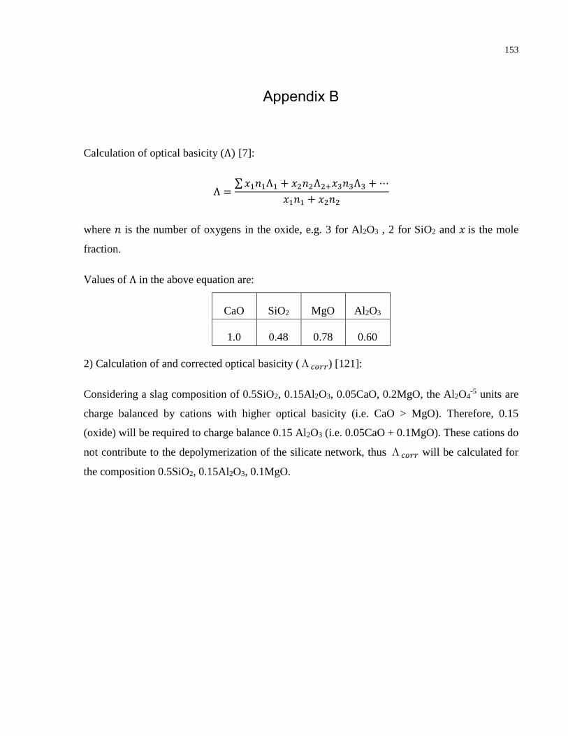
153

Appendix B

Calculation of optical basicity (Λ) [7]:

Λ =∑ 𝑥1𝑛1Λ1 + 𝑥2𝑛2Λ2+𝑥3𝑛3Λ3 + ⋯

𝑥1𝑛1 + 𝑥2𝑛2

where 𝑛 is the number of oxygens in the oxide, e.g. 3 for Al2O3 , 2 for SiO2 and 𝑥 is the mole

fraction.

Values of Λ in the above equation are:

CaO SiO2 MgO Al2O3

1.0 0.48 0.78 0.60

2) Calculation of and corrected optical basicity (Λ𝑐𝑜𝑟𝑟) [121]:

Considering a slag composition of 0.5SiO2, 0.15Al2O3, 0.05CaO, 0.2MgO, the Al2O4-5 units are

charge balanced by cations with higher optical basicity (i.e. CaO > MgO). Therefore, 0.15

(oxide) will be required to charge balance 0.15 Al2O3 (i.e. 0.05CaO + 0.1MgO). These cations do

not contribute to the depolymerization of the silicate network, thus Λ𝑐𝑜𝑟𝑟 will be calculated for

the composition 0.5SiO2, 0.15Al2O3, 0.1MgO.

Crystallization of Synthetic Blast Furnace Slags …...Crystallization of Synthetic Blast Furnace...

Documents

Transcript of Crystallization of Synthetic Blast Furnace Slags …...Crystallization of Synthetic Blast Furnace...