Cruise Report COPAS’08 R/V Revelle Cruise Number Knox22RR William M. Balch (chief scientist) Bigelow Laboratory for Ocean Sciences POB 475 W. Boothbay Harbor, ME 04575 Science Party (arranged alphabetically): Dr. John Allen, National Oceanography Centre, Southampton, U.K. Nicole Benoit, Woods Hole Oceanographic Inst., Woods Hole, MA Bruce Bowler, Bigelow Laboratory for Ocean Sciences, Bigelow Laboratory for Ocean Sciences, W. Boothbay Hbr., ME Kate Callnan, (Laboratory of Dr. Lisa Moore), University of Southern Maine, Portland, ME Tyler Cyronak, College of Charleston, Charleston, SC Dr. Jack Ditullio, College of Charleston, Charleston, SC Laura Daniels (laboratory of Dr. M. Débora Iglesias-Rodriguez), National Oceanography Centre, Southampton, UK. Dave Drapeau, Bigelow Laboratory for Ocean Sciences, W. Boothbay Hbr., ME Marlene Jeffries, (Laboratory of Nick Bates) Bermuda Institute of Ocean Science, Marine Biogeochemistry Lab Jeff Lawrence, Armada teacher, Lowrey School, Tahlequah, OK Dr. Peter Lee, College of Charleston, Charleston, SC Barbara Lyon, College of Charleston, Charleston, SC Laura Lubelczyk, (Laboratory of Dr. William Wilson) Bigelow Laboratory for Ocean Sciences Emily Lyskowski, Bigelow Laboratory for Ocean Sciences, Bigelow Laboratory for Ocean Sciences, W. Boothbay Hbr., ME Charlotte Marcinko, National Oceanography Centre, Southampton, U.K. Dr. Joaquin Martinez Martinez (Laboratory of Dr. William Wilson) Bigelow Laboratory for Ocean Sciences, Bigelow Laboratory for Ocean Sciences, W. Boothbay Hbr., ME Dr. Stuart Painter, National Oceanography Centre, Southampton, U.K. Roz Pidcock, National Oceanography Centre, Southampton, U.K. Dr. Alex Poulton, National Oceanography Centre, Southampton, U.K. Ricardo Silva, Instituto Nacional de Investigacion y desarrollo pesquero, Paseo Victoria Ocampo #1, Mar del Plata, Argentina Dr. Silvia Romero, Servicio de Hidrografía Naval, Argentina Dr. Maria Saggiomo, Stazione Zoologica A. Dohrn – Napoli – Italy Dr. Immacolata Santarpia, Stazione Zoologica A. Dohrn – Napoli – Italy Martha Valiadi , National Oceanography Centre, Southampton, U.K. Daniel Valla, Universidad de Buenos Aires, Argentina Heather A. Wright, Univ. Southern Maine, Portland, ME STS Personnel, SIO Matt Durham, SIO Res. tech Bud Hale, SIO, computing Rob Palomares, SIO Res. Tech Dan Schuller, SIO, chemistry Dan Yang , SIO, computing

Introduction The COPAS (Coccolithophores of the Patagonian Shelf) expedition embarked

aboard R/V Roger Revelle from Montevideo Uruguay on 4 December 2008 on cruise number Knox22RR. The cruise track is shown in figure 1, which overlays a MODIS Aqua “true color” satellite image from 10 December 2008 (produced by Mr. Norman Kuring, NASA Goddard Space Flight Center, Greenbelt, MD). Labels have been tentatively given for different algal populations that we observed on the trip, based on microscopy and flow-cam analyses. Our first line out of Montevideo was meant to cross the Malvinas/Falklands Current well north of the coccolithophore bloom. We then tracked obliquely across the shelf break zone, observing the first dense populations of coccolithophores at ~42oS. Fig. 1- True-color AQUA MODIS image of the SW Atlantic off of Argentina and the Falklands/Malvinas Islands (10 December

2008; processed by Norman Kuring, NASA, Goddard Space Flight Center). While no community was unialgal, the turquoise waters were almost exclusively coccolithophorids, plus healthy numbers of Synechococcus, with spectacularly high albedo and turbidity (objects cannot be seen within 1-2 meters of the surface). These blooms were right in the middle of the Malvinas/Falklands current (based on T/S signature), with low to undetectable silicate, and nitrate (commensurate with high nutrient/low chlorophyll waters). Ship’s ADCP and daily satellite imagery showed strong northerly mean advection of the coccolithophore populations along the shelf break. We observed the growth and gradual demise of the feature during the cruise. Dilution experiments demonstrated significant grazing mortality. Huge populations of dolliolid salps also were observed in the water in the coccolithophore bloom. As the water is advected to the northeast, the coccolithophores gave way to mixed dinoflagellates and flagellates (apparent as a change to deeper green in the true color image). Deep populations of Prochlorococcus were found offshore in the northern part of the study area (obviously not visible to the satellite). The dinoflagellate population north of the Falklands/Malvinas had extremely high chlorophyll, and contained Prorocentrum minimum. On the eastern side of the coccolithophore bloom was a mixed population of diatoms, dinoflagellates and coccolithophores. The coccolithophore bloom, south of the Falklands/Malvinas, appeared to be growing rapidly and had low numbers of detached coccoliths per plated cell.

When the R/V Roger Revelle reached the first dense populations of coccolithophores, we steamed a radiator grid until we reached the brightest portion of the bloom, just north of the Falkland/Malvinas Islands. Then we “connected the grid” by steaming up the main axis of the bloom, crossing several stations that we had previously sampled. We then returned back down the same line, crossing the same stations again. Thus, we sampled the densest portion of the bloom three times providing insights into its changes in space and time.

The station plan generally had CTD stations at 30km resolution over the entire cruise, except for the first line from Montevideo (in which stations were further apart as the science party became more adept at running casts and processing water. After the first line was complete, a long diagonal line was run in a SW direction, with water sampling every station. For all subsequent stations, every other station was processed for a full water cast and CTD profile. The station design always placed the full stations at corners of the transit patterns. This station plan translated to a total of 152 stations, with 76 full-cast water stations. The CTD was equipped with an oxygen sensor and beam transmissometer (at 660nm). Stand-alone pumps (SAPS) were deployed at varying parts of the cruise, with two water depths sampled. A hand-deployed light meter was deployed daily at local apparent noon, weather conditions permitting. This provided spectral estimates of the diffuse attenuation. Experiments on ocean acidification were performed in deck incubators in ambient seawater tanks.

A total of 168 CTD profiles at 152 stations were completed on cruise

KNOX22RR, including 25 dawn primary productivity casts. Depths of the profiles varied from less than 10 m for carboy experiments to a maximum of 5204 m. Most casts, however, extended to 1000 m offshore and were limited by topography along the shelf break and inshore. Profile casts down to 1000 m were interspersed with water casts to increase the along-track resolution of the hydrographic data and to resolve the deeper structure beyond the euphotic zone. On such casts, water was not sampled. On casts where water was taken, sampling from Niskin bottles took place in the following order: oxygen, DIC/Alk, DMS, DOC, nutrients, primary productivity, PIC/POC/Chl, cyanobacteria distribution, HPLC, virus abundance, salts. Sampling was carried out at the following fixed light depths: 50%, 30%, 20%, 10%, 5%, 3%, 1%, 0.1%. These were calculated based on one of two methods: a) during the day, percentages of surface irradiance taken from the downcast profile immediately preceding bottle firing or b) at night, based on the measured beam transmittance and previously determined relationships between beam transmittance and diffuse attenuation of photosynthetically available radiation (PAR).

The cruise terminated in Punta Arenas, Chile, and offloading was complete by 5

January 2009.

Ocean optics, phytoplankton standing stocks, ocean acidification experiments Dr. William Balch, Bigelow Laboratory for Ocean Sciences Dave Drapeau, Bigelow Laboratory for Ocean Sciences Bruce Bowler, Bigelow Laboratory for Ocean Sciences Emily Lyskowski, Bigelow Laboratory for Ocean Sciences Heather-Anne Wright, (laboratory of Dr. Lisa Moore), Univ. Southern Maine Jeff Lawrence, Armada teacher, Lowrey School, Tahlequah, OK

The Balch lab was involved in sampling a number of variables from the bottle casts, running an optical surface underway system and it also coordinated the carboy experiments and dilution experiments on ocean acidification. We sampled from 76 CTD stations during the cruise, taking water from 8 of the 12 bottles each cast. Water samples were taken for particulate organic carbon (POC) and particulate organic nitrogen (PON), particulate inorganic carbon (CaCO3 or PIC), biogenic silica, coccolithophore counts (processed using the Canada Balsam technique for enumeration of calcite particles), chlorophyll a extractions (surface bottles always run in triplicate), and flow-cam samples (for enumeration of net and nanoplankton). The bio-optical underway system was run continuously over the course of the trip. This system has been described elsewhere [Balch et al., 2008]. Basically it measures temperature, salinity, chlorophyll a fluorescence and backscattering at 531nm (using a WETLabs ECOVSF sensor). At a period determined by the operator, 10% glacial acetic acid was injected into the flow stream, upstream of the ECOVSF to reduce the pH to 5.4-5.5, below the dissociation point for calcium carbonate. A pH sensor downstream of the sample chamber measured the pH and sent this information to the acid controller. Once 60 seconds (or whatever was required for a statistically-significant measurement) of data were collected with ambient pH, the acid controller injected 0.2um-filtered glacial acid into the seawater stream, passing through a mixing coil to thoroughly mix it with the seawater. Once the pH dropped to pH 5.4, the backscattering was re-measured for 60s. The difference in backscattering represented acid-labile backscattering, which can be directly related to the concentration of suspended calcium carbonate. The flow-through system had a separate loop that passed through a WETLabs ac-9. In the flow path to the ac-9 was a solenoid that diverted the seawater stream through a 1μm filter, then a 0.2 μm filter prior to running the water through the ac-9. Every two minutes, the solenoid would alternate between filtered and unfiltered seawater, thus providing absorption and attenuation (at 9 spectral wavelengths across the visible spectrum) for raw and filtered seawater (thus providing the absorption and attenuation of total suspended particles and dissolved particles).

On the bow of the R/V Roger Revelle was a Satlantic SeaWiFS Aircraft Simulator (MicroSAS) system, used to estimate water-leaving radiance from the ship, analogous to to the nLw derived by the SeaWiFS and MODIS satellite sensors, but free from atmospheric error (hence, it can provide data below clouds). The system consisted of a down-looking radiance sensor and a sky-viewing radiance sensor, both mounted on a steerable holder on the bow. A downwelling irradiance sensor was mounted at the top of the ship’s meterological mast, on the bow, far from any potentially shading structures. These data were used to estimate normalized water-leaving radiance as a function of

wavelength. The radiance detector was set to view the water at 40o from nadir as recommended by Mueller et al. [2003b]. The water radiance sensor was able to view over an azimuth range of ~180o across the ship’s heading with no viewing of the ship’s wake. The direction of the sensor was adjusted to view the water 90-120 o from the sun's azimuth, to minimize sun glint. This was continually adjusted as the time and ship’s gyro heading were used to calculate the sun's position using an astronomical solar position subroutine interfaced with a stepping motor which was attached to the radiometer mount (designed and fabricated at Bigelow Laboratory for Ocean Sciences). Protocols for operation and calibration were performed according to Mueller [Mueller et al., 2003a; Mueller et al., 2003b; Mueller et al., 2003c]. Before 1000h and after 1400h, data quality was poorer as the solar zenith angle was too low. Post-cruise, the 10Hz data were filtered to remove as much residual white cap and glint as possible (we accept the lowest 5% of the data). Reflectance plaque measurements were made several times at local apparent noon on sunny days to verify the radiometer calibrations.

Within an hour of local apparent noon each day, a Satlantic OCP sensor was

deployed off the stern of the R/V Revelle after the ship oriented so that the sun was off the stern. The ship would secure the starboard Z-drive, and use port Z-drive and bow thruster to move the ship ahead at about 25cm s-1. The OCP was then trailed aft and brought to the surface ~100m aft of the ship, then allowed to sink to 100m as downwelling spectral irradiance and upwelling spectral radiance were recorded continuously along with temperature and salinity. This procedure ensured there were no ship shadow effects in the radiometry. Carboy Experiments

Five carboy experiments were performed during the 28d cruise. The purpose of the experiments was to assess the impact of different concentrations of pCO2 on various aspects of the phytoplankton community. At each time point, samples were taken for: pH, nutrients (nitrate, nitrite, ammonium, phosphate and silicate), alkalinity, total dissolved inorganic carbon, coccolithophore abundance, chlorophyll a, PIC, biogenic silica, and flow-cam-determined abundance (and associated plasma volume). Other samples also were taken for flow cytometric counts, dissolved DMS, DOC, phytoPAM, primary production, calcification and HPLC pigments. Each experiment involved collecting 360L of seawater from about 5m depth using the 30-L Niskin bottles attached to the ship’s CTD rosette. The Niskin bottles were equipped with silicone O-rings. When the CTD was recovered, seawater was gravity fed from the Niskin bottles via silicone tubing connected to 8 of the Niskin bottles, through a single manifold (in order to mix the water from all bottles equally) and then re-partitioned into 8 20L polycarbonate carboys which were gently filled in subdued light. The four remaining Niskin bottles were connected to a four-way manifold using silicon tubing, then directed through a 0.2 um filter. A pneumatic pump was used to slowly filter this water into four carboys to be used as non-particle controls. Once filled, any remaining water in the Niskin bottles was used for time-zero samples. All carboys were then placed in blue seawater incubators (cooled with surface ambient seawater) and covered with neutral-density screen (which reduced the total

irradiance to 58% of incident). Each carboy was connected to a gas manifold that circulated CO2/air mixtures into them. The flow rates of gas into each carboy were ~100 ml min-1, and were directed through a length of silicone tubing and an “air-stone” at the bottom of the carboy to finally aerate the seawater. This level of aeration was not harsh relative to the turbulence induced by the rolling of the ship, and insured rapid equilibration. Gas outflow passed through the carboy headspace, through a separate tube with 0.2μm filter to prevent atmospheric contamination. The CO2/air concentrations used in this experiment were 380, 500, 750 and 1200 ppm (supplied by Scott Marin, Riverside, CA). Time points were at zero time, 24h and 72h. At 48h, a reduced sample was taken only for pH and DIC. The filtered control carboys were sampled for pH, alkalinity and total dissolved inorganic carbon, in order to assess the physical/chemical aspects of the bubbling, free from biology. Dilution experiments Dilution experiments were performed from two of the pCO2 concentrations (380 and 750ppm) using water one of the replicate carboys, mixed with water from the filtered-seawater carboy. The method of Landry and Hassett [Landry and Hassett, 1982] was used. Water was carefully siphoned from the carboys after 24h, and dispensed gently into each 2L polycarbonate bottle. Each bottle was equipped with a piece of silicon tubing, air-stone with gentle gas flow, in order to maintain the pCO2 concentration at the same level that the seawater had in the carboys. The dilution bottles were incubated in the same seawater incubator that held the carboy experiments. The 24h samples from the respective carboys provided the T-initial measurements for the dilution experiments, after correcting for the appropriate dilution. The dilutions that were used in the experiments were: 100%, 100% plus 12μM nitrate (a control to assess for nitrogen limitation in the most concentrated sample), 75%, 50%, 25% and 0%. After the dilution bottles had incubated 24h (representing t-48 of the carboy experiments), the dilution experiments were terminated. Samples for pH, nutrients, chlorophyll a, coccolithophore counts, Flow-cam counts, PIC and BSi were taken along with flow cytometry counts, DMS measurements and HPLC pigments measurements. Sample volume We performed five carboy and dilution experiments over the cruise, and sampled all water casts. Underway samples were also taken at 6 stations to document interesting features. In total, 799 water samples were processed for all variables listed above: 75 were for carboy experiments, 60 for dilution experiments, 6 underway samples (targetting specific features observed on the underway system and 658 CTD Niskin bottles). References Balch, W.M., D.T. Drapeau, B.C. Bowler, E.S. Booth, L.A. Windecker, and A. Ashe

(2008), Space-time variability of carbon standing stocks and fixation rates in the Gulf of Maine, along the GNATS transect between Portland, ME and Yarmouth, NS., Journal of Plankton Research, 30 (2), 119-139.

Landry, M.R., and R.P. Hassett (1982), Estimating the grazing impact of marine micro-zooplankton, Marine Biology, 67, 283-288.

Mueller, J.L., R.W. Austin, A. Morel, G.S. Fargion, and C.R. McClain (2003a), Ocean optics protocols for satellite ocean color sensor validation, Revision 4, Volume I: Introduction, background, and conventions, pp. 50, Goddard Space Flight Center, Greenbelt, MD.

Mueller, J.L., A. Morel, R. Frouin, C. Davis, R. Arnone, K. Carder, Z.P. Lee, R.G. Steward, S.B. Hooker, C.D. Mobley, S. McLean, B. Holben, M. Miller, C. Pietras, K.D. Knobelspiesse, G.S. Fargion, J. Porter, and K. Voss (2003b), Ocean optics protocols for satellite ocean color sensor validation, Revision 4, Volume III: Radiometric measurements and data analysis protocols, pp. 78, Goddard Space Flight Center, Greenbelt, MD.

Mueller, J.L., C. Pietras, S.B. Hooker, R.W. Austin, M. Miller, K.D. Knobelspiesse, R. Frouin, B. Holben, and K. Voss (2003c), Ocean optics protocols for satellite ocean color sensor validation, Revision 4, Volume II: Instrument specifications, characterization,and calibration, Goddard Space Flight Center, Greenbelt, MD.

DIC and Alkalinity Marlene Jeffries, (Laboratory of Dr. Nick Bates) Bermuda Institute of Ocean Science, Marine Biogeochemistry Lab Nicole Benoit, Woods Hole Oceanographic Inst., Woods Hole, MA

The Bates group participated in the COPAS'08 research cruise to (1) investigate the carbonate chemistry of the Patagonia Shelf and the effects of CO2 uptake by large coccolithophore blooms; (2) provide the carbonate chemistry for high-CO2 incubation experiments. In addition, we used a SAMI underway pCO2 sensor throughout the cruise to measure pCO2 from the underway seawater system. Method of sampling

The DIC/TA samples were drawn from each Niskin bottle using a 200ml glass bottle. Filling from the bottom eliminates bubbles and leaving a minimal headspace in the neck of the bottle allows the sample to be returned to the lab for analysis. The headspace in the bottle contributes to error in the sample which is less than the precision of the VINDTA (~ ± 4 μmoles/kg). Each sample was then poisoned with 100 ml of mercuric chloride to eliminate further biological effects on the sample. DIC and Alkalinity Samples

In total, 1110 DIC/TA samples were taken over the duration of the the COPAS'08 research cruise. From the rosette, 895 samples were taken from each bottle cast at various depths. From the underway seawater system, 32 samples were drawn. From the high-CO2 carboy experiments, 183 DIC/TA samples were drawn at times T0, T24, T48 and T72. Underway pCO2 system.

A SAMI underway pCO2 sensor was also installed on the underway seawater system. The SAMI samples at 15 minutes intervals and ran for the duration of the cruise, with the exception of 2 days where the data logger locked up. Surface DIC/TA samples were drawn from the underway system (32 in total) to ground truth the SAMI pCO2 data. The underway pCO2 data will be finalized once the surface samples are analyzed.

Physics data processing Dr. John Allen, National Oceanography Centre, Southampton, U.K. Dr. Stuart Painter, National Oceanography Centre, Southampton, U.K. Dr. Silvia Romero, Servicio de Hidrografía Naval, Argentina Roz Pidcock, National Oceanography Centre, Southampton, U.K. Daniel Valla, INIDEP, Argentina Charlotte Marcinko, National Oceanography Centre, Southampton, U.K. CTD Sampling, Processing and Calibration

Water sampling consisted of a total of 168 CTD profiles at 152 stations, including 25 dawn productivity casts. Depths of the profiles varied from less than 10m for carboy experiments to a maximum of 5204 m. Most casts, however, extended to 1000 m offshore and were limited by topography along the shelf break and inshore. Profile casts down to 1000 m were interspersed with water collection casts to increase the along-track resolution of the hydrographic data and to resolve the deeper structure beyond the euphotic zone. On such casts, water was not sampled. SeaBird Processing Data was acquired using SeaBird SeaSave v7 for SBE 911 software. Following each cast, data acquisition was stopped and saved to the deck unit PC. The logging software output four files per cast with the following forms: nnnnn.hex (raw data file), nnnnn.con (data configuration file), nnnnn.bl (contained record of bottle firing locations and nnnnn.hdr (header file), where ‘nnnnn’ was the 3-digit station number followed by the 2-digit cast number. The output files were backed up to the file location rv-revelle/cruise-data/KNOX22RR-share/CTD-process. The raw data files were then processed using SeaBird SBE.DataProcessing software version 7.18b according to Scripps Institute protocol. Output files from the SeaBird processing were of the form nnnnn.cnv (binary up and down casts), nnnnn.btl and nnnnn.ros (bottle firing information). Following SeaBird processing, the output files were copied to /noc/users/pstar/mstar/mexec/data/ctd/processed on the UNIX workstation Osiris. Processing was continued within MStar, a Matlab library of scripts developed from the historical Pstar fortran based oceanographic processing library previously used by IOSDL, the James Rennel Centre and NOCs, and using the following routines: ctd0: This converts the 24Hz SeaBird .cnv file into netCDF format, setting the required

header information. Output: ctd22RRnnnnn_24Hz ctd1: This carries out a de-spike on the .24Hz data and averages it into a 1Hz file,

(ctd22RRnnnnn_1Hz). Salinity, potential temperature and density are derived from the primary and secondary temperature and conductivity sensors. Finally a 10 second averaged file is created, (ctd22RRnnnnn_10s)

ctd2: Requires the user to find the first in-water, deepest and last in-water data-cycle from the .1Hz file. These scripts then extract data to correspond to the full up and down casts (ctd22RRnnnnn.ctu file) and purely the downcast (ctd22RRnnnnn.2db), averaged into 2db bins.

fir0: This converts the .ros file into netCDF format. It then takes relevant data-cycles from the .10s averaged file and pastes them into a new file fir22RRnnnnn containing the mean values of all the variables at the bottle firing locations.

samfir: This creates a master samnnnnn file for the cast and pastes in selected variables from the fir22RRnnnnn file. sal0: Reads in the sample bottle excel text files into MStar format. Output file:

salnnnnn. passal: Merges bottle file values from salnnnnn into sam22RRnnnnn file. Output file:

sam22RRnnnnn. botcond: Calculation of conductivities from salinometry (bottle) salinities. Result added

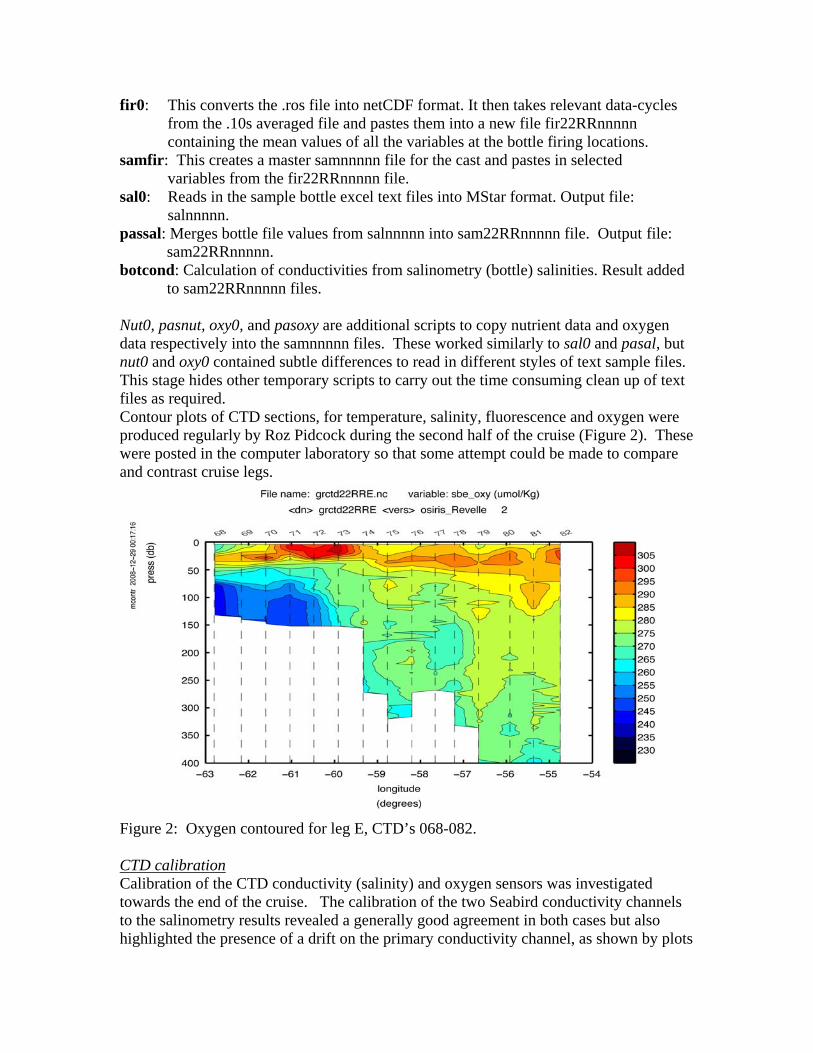
to sam22RRnnnnn files. Nut0, pasnut, oxy0, and pasoxy are additional scripts to copy nutrient data and oxygen data respectively into the samnnnnn files. These worked similarly to sal0 and pasal, but nut0 and oxy0 contained subtle differences to read in different styles of text sample files. This stage hides other temporary scripts to carry out the time consuming clean up of text files as required. Contour plots of CTD sections, for temperature, salinity, fluorescence and oxygen were produced regularly by Roz Pidcock during the second half of the cruise (Figure 2). These were posted in the computer laboratory so that some attempt could be made to compare and contrast cruise legs.

Figure 2: Oxygen contoured for leg E, CTD’s 068-082. CTD calibration Calibration of the CTD conductivity (salinity) and oxygen sensors was investigated towards the end of the cruise. The calibration of the two Seabird conductivity channels to the salinometry results revealed a generally good agreement in both cases but also highlighted the presence of a drift on the primary conductivity channel, as shown by plots

of conductivity difference against station number (i.e. time). This suggests that conductivity 2 and temperature 2 will provide more reliable estimates of salinity although the overall impact of the drift on the primary channel remained small. SeaBird claim that the correct in-situ calibration for their conductivity sensors is a linear function of conductivity with no offset. Plots of conductivity difference against conductivity added support to this and therefore the calibration coefficients A and B were calculated as

A =CondbotCondctd∑

Condctd( )2∑=

CondbotCondctd

Condctd( )2

and

B =Cond2bot Cond2ctd∑

Cond2ctd( )2∑=

Cond2bot Cond2ctd

Cond2ctd( )2

where cond is the sample bottle conductivity determined with the secondary temperature variable.

2bot

Coefficient A was determined to be 1.000177 and coefficient B was determined to be 1.000096. Corrected Seabird conductivities was calculated through the application of coefficient A to primary conductivity and coefficient B to the secondary conductivity channel. Residual conductivity differences were calculated as bottle conductivity – corrected Seabird conductivity. On conductivity channel 1 the mean residual was calculated as -0.00051 S/m and the standard deviation was 0.00275. On conductivity channel 2 the mean residual was -0.00017 S/m and the standard deviation was 0.00216. The linear regression between Seabird 43 oxygen concentrations (in ml/l) and manual titrations produced a regression equation of y = 1.048204 * SBEoxy + 0.058575 where y = corrected oxygen concentration. The typical range of residual values (i.e. corrected Seabird oxygen concentration – bottle titration estimate) was ±0.06 ml/l. The mean residual estimate however was 0.0036 ml/l with a standard deviation of 0.0395, suggesting an accuracy typically < 1% of oceanic oxygen concentrations. 150kHz Vessel Mounted Acoustic Doppler Current Profiler

The RV Roger Revelle was equipped with an RDI 150 kHz narrowband ADCP that was interfaced with the University of Hawaii Data Acquisition System (UHDAS) and the CODAS (Common Ocean Data Access System) database. Consequently ADCP data can be made available to onboard scientists via an automated processing system. The data were made available in three forms, raw ping data (via the CODAS database),

processed 5 minute ensemble data (corrected for ships motion) and a 15 minute average calculated from the 5 minute ensemble data. The latter two products were obtained as Matlab compatible files.

Much of the UHDAS system is intentionally hidden from the casual user and thus the system is best left to work as pre-set. The standard data acquisition configuration, whereby the ADCP was configured to sample with 8 m depth resolution and 5 minute averaging, was thus used throughout the cruise. Email contact with Dr. Julia Hummon at the University of Hawaii during the early stages of the cruise answered some of our initial questions and a thorough post cruise analysis of the data was undertaken to remove anomalous velocity measurements which the automated processing system may have occasionally left in the data. Aspects of this process required use of the CODAS processing system which could not be adequately set up during the cruise.

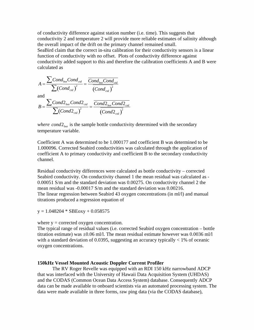
During a period of bad weather around year day 356 (Dec 21st) the ADCP stopped working for approximately 36 hrs. This unfortunately was not noticed during the daily visual checks of the ADCP deck unit nor within the processed data files as the CODAS database system was unaffected and continued to write new 15 minute averaged files at regular intervals; only without new data being appended. This was a regrettable oversight. Fortunately the survey line affected was resurveyed, so whilst temporal data may have been lost this was not at the cost of spatial understanding. Initial interpretation of the ADCP data (Figure 3) suggests a strong signal exists for the shelf break currents that exist between the 200 and 1000 m bathymetry contours.

Figure 3: Preliminary velocities along the Patagonian Shelf break, north of the Falklands/Malvinas Islands. Also shown are the 200 m (green), 500 m (red) and 1000 m (blue) bathymetry contours. Navigation/Heading/Gyro Introduction

On the R/V Roger Revelle, the primary scientific navigation instrument is a Furono GP90. The data from this, the now standard Ashtech 3D GPS, and the ship’s gyro were fed to processing systems around the ship by NMEA messages $GPGGA, $PASHR and $GPVTG. Detailed processing of the ashtech data was not required as this is handled by the SCRIPPS/Univ. Hawaii automated VM-ADCP and HDSS processing systems where required. So what follows is simply a description of the acquisition of the data for processing in the NOCS Mstar (the new MATLAB/NetCDF based re-incarnation of Pstar) system for updating the bottom position for CTD files and as a back-up for further analysis of ADCP/HDSS data if required in the future.

Offline Mstar data handling The NMEA data streams were recorded as part of the ship’s computing system in daily files. The Ashtech daily files, e.g. ASHinpf.2008dec15, had the advantage that they contained all three of the $GPGGA, $PASHR and $GPVTG messages. However, on the last day of the cruise the Ashtech acquisition system failed for a period of just over 2 hours and therefore a section from the GP90inpf.2008dec31 file (containing only $GPGGA and $GPVTG streams) had to be stitched in manually during our Mstar processing described below. These NMEA archive files were transferred to the NOCS LINUX worstation ‘osiris’ where all the master Mstar processing was carried out. Scripts: navexec0: Transferred data from the nmea stream format to Mstar NetCDF files

(nmea_to_mstar.m script), and calculated time difference between datacycles to check for the size of gaps and any backward timesteps. Output nav22RRnnraw file.

ashexec: Calculated the difference between Ashtech and gyro heading and re-ranged this to the range -180 to 180 degrees. Edited out likely bad data on the basis of:

-5 < pitch < 5 -7 < roll < 7 -10 < ash-gyro < 10 later changed to -20 < ash-gyro <20 Further editing of the data was carried out with a median despike, before averaging to 1minute intervals. Further editing of the 1 minute file followed removal of data where: -4 < roll < 4 and later -15 < ash-gyro < 10

Speed and direction were calculated in the 1 minute average file and spot gyro values were merged in from the edited but not averaged 1 second file. Two outputs, ash22RRnn.nc and ash22RRnnav.nv files Navexec1: Appended nav22RRnnraw files into the file nav22RR1sec, losing the time

difference variable. Re-create time difference just to double-check for problems at the ends of individual files. Average to a 1 minute navigation file, more useful to the majority of colleagues. Interpolate over short time gaps, the largest allowed during this cruise was 254 seconds. As mentioned earlier, a large gap over 8000 seconds during the last file of the cruise was repaired before appending. After plotting to visually check there were no oddities, distance run was calculated for the 1 minute averaged file. An ascii file was created from the 1 minute navigation NetCDF file early each morning.

Sampling for HPLC, flow cytometry, phytoPAM, DMS, and domoic acid Dr. Jack Ditullio, College of Charleston, Charleston, SC Dr. Peter Lee, College of Charleston, Charleston, SC Tyler Cyronak, College of Charleston, Charleston, SC Barbara Lyon, College of Charleston, Charleston, SC Dr. Immacolata Santarpia, Stazione Zoologica A. Dohrn – Napoli – Italy Dr. Maria Saggiomo, Stazione Zoologica A. Dohrn – Napoli – Italy 1. CTD Stations (even-numbered)

1.1. HPLC Pigment samples were collected at 8 depths in the photic zone (down to the 0.1% light level). 1.2. Size-fractionated HPLC pigment samples (using 20um, 2um and GF/F

filters) were collected at all stations at two depths (near surface and chl max) 1.3. Phyto-PAM samples were analyzed at four depths (near surface, chl max and two intermediate depths). 1.4. Photosynthetic efficiency of PSII in the photic zone were measured at all

stations. 1.5. Flow cytometry samples were analyzed and/or preserved from all stations

1.6. Approximately 12 profiles (8 depths) were collected for the analyses of particulate methyl mercury.

1.7. Samples were taken for the measurement of dissolved organic carbon at approximately 15 stations, with samples collected in both surface and deep water.

1.8. Measurements of DMS were made at most stations and samples were preserved for the analyses of both dissolved and particulate DMSP from all stations.

1.9. Samples were collected for the analysis of domoic acid at approximately 12 coastal stations.

2. Underway Sampling

2.1. Continuous underway measurements of Fv/Fm and other photosynthetic parameters. 2.2. Approximately 120 underway surface samples were collected for HPLC Pigment, Phyto-PAM and DMSP analyses.

3. Carboy CO2 Incubation Experiments

3.1. Flow Cytometry samples preserved from all 5 experiments 3.2. DMSP samples collected and preserved from all 5 experiments 3.3. HPLC pigment samples were collected from both dilution expts and Tfinal

from all five incubation experiments. 3.4. Photosynthetic efficiency of PSII and other photosynthetic parameters taken

from all 5 incubation experiments.

4. CO2 Effects on DOC Concentration 4.1. Two experiments performed on CO2 effects on DOC concentrations. Samples were collected for DOC analyses from 380ppm and 750 ppm treatments.

4.2. Samples preserved for bacterial composition analyses (using DGGE) 5. Flow Cytometry Sorting

5.1. Various samples were sorted for ROS measurements (w/ Joaquin) 5.2. Various populations were sorted to determine intracellular concentrations of

DMSP and accessory pigments. 5.3. Various populations were sorted for genetic analyses. 5.4. Various populations were sorted for epifluorescence/SEM microscopy 5.5. Various populations were collected for culturing 5.6. Various Prochlorococcus and Synechococcus populations were sorted for

Kate Callnan (i.e. working for Dr. Lisa Moore, Univ. S. Maine).

Primary production and calcification

Dr. Alex Poulton, National Oceanography Centre, Southampton, U.K.

Daily rates (dawn-to-dawn, 24-hrs) of primary production (PP) and calcification

(CF) were determined at 25 CTD stations and during 5 pCO2 experiments following the methodology of Paasche & Brubak (1994) and Balch et al.(2000). Water samples (150-ml, 3 light, 1 formalin-killed) were collected from 6 light depths (50, 30, 11, 7, 5, 1.5% incident light), spiked with 60-70 μCi of 14C-labelled sodium bicarbonate and incubated on deck. On deck incubators were chilled with sea surface water and light depths were replicated through the use of a mixture of misty blue and grey light filters. Incubations were terminated by filtration through 25-mm 0.2-μm polycarbonate filter, with extensive rinsing with fresh filtered seawater to remove any labeled 14C-DIC. Filters were then placed in glass vials with gas-tight septum and a bucket containing a Whatman GFA filter soaked in phenylethylamine (PEA) attached to the lid. Phosphoric acid (1 ml, 1%) was injected through the septum into the bottom of the vial to convert any labeled 14C-PIC to 14C-CO2 which was then caught in the PEA soaked filter. After 20-24-hrs, GFA filters were removed and placed in fresh vials and liquid scintillation cocktail was added to both vials: one containing the polycarbonate filter (non-acid labile production, organic or primary production) and one containing the GFA filter (acid-labile production, inorganic production or calcification). Activity in both filters was then determined on a liquid scintillation counter and counts converted to uptake rates using standard methodology. Each measurement of calcification was matched with: (1) a sample for the determination of coccolithophore cell numbers and species identification by light microscopy (200-400 ml filtered through a 0.45-μm cellulose nitrate filter, oven dried at 50-60oC for 10-12 hrs and stored in petri-slides; n = 200); and (2) a sample for the determination of coccolithophore cell calcite by scanning electron microscopy (300-600 ml filtered through a 0.45-μm polycarbonate filter, oven dried at 50-60oC for 10-12 hrs and stored in petri-slides; n = 200). References Balch, W.M., Drapeau, D.T., Fritz, J.J., 2000, Monsoonal forcing of calcification in the Arabian Sea, Deep-Sea Research II, 47, 1301-1337. Paasche, E., Brubak, S., 1994, Enhanced calcification in the coccolithophorid Emiliania huxleyi (Haptophyceae) under phosphorus limitation, Phycologia, 33, 324-330.

Table 1. List of stations sampled for primary production (PP) and calcification (CF).

PP Identifier Station no. Date

PP-01 005/01 6 Dec 2008 PP-02 008/02 7 Dec 2008 PP-03 010/02 8 Dec 2008 PP-04 014/01 9 Dec 2008 PP-05 017/01 10 Dec 2008 PP-06 020/01 11 Dec 2008 PP-07 025/01 12 Dec 2008 PP-08 032/01 13 Dec 2008 PP-09 040/01 14 Dec 2008 PP-10 047/02 15 Dec 2008 PP-11 052/02 16 Dec 2008 PP-12 060/01 17 Dec 2008 PP-13 068/01 18 Dec 2008 PP-14 072/01 19 Dec 2008 PP-15 078/02 20 Dec 2008 PP-16 086/01 21 Dec 2008 PP-17 090/01 22 Dec 2008 PP-18 094/01 23 Dec 2008 PP-19 102/01 24 Dec 2008 PP-20 108/01 25 Dec 2008 PP-21 116/01 26 Dec 2008 PP-22 122/01 27 Dec 2008 PP-23 128/01 28 Dec 2008 PP-24 134/01 29 Dec 2008 PP-25 142/01 30 Dec 2008

Genetic Diversity and transcriptional profiles Dr. Joaquin Martinez Martinez (Laboratory of Dr. William Wilson) Bigelow Laboratory for Ocean Sciences Laura Lubelczyk, (Laboratory of Dr. William Wilson) Bigelow Laboratory for Ocean Sciences During the COPAS cruise we collected samples to study genetic diversity and transcriptional profiles of phytoplankton species and viruses during a coccolithophore-dominated bloom along the Patagonian Shelf. We focused on the host-virus system of Emiliania huxleyi-. At all the water stations we collected water at 6 to 12 depths for the following purposes:

‐ Bacteria and virus abundance counts by Flow Cytometry (FCM) ‐ DNA preparations for investigation of genetic richness of Emiliania huxleyi and

viruses that infect them. In addition, we also collected one filter for DNA preparation using the SAPS at 1000 m.

At every productivity station, in addition to the samples above, we collected for the following purposes:

‐ Lipids analysis from surface, chlorophyll maximum and just below the chlorophyll maximum.

‐ Group specific virus sorting for subsequent molecular analysis (same depths as for lipids analysis).

‐ New phytoplankton virus isolation (only at selected stations and depths).

From the carboy experiments we collected water at T0, T24 and T72 from all CO2 pressures for the following purposes:

‐ Bacteria and virus abundance counts by FCM from each of the carboys. At T0 we sampled both unfiltered and filtered water.

‐ DNA preparations for investigation of genetic richness of Emiliania huxleyi and viruses that infect them from carboy numbers 1, 4, 7 and 10.

‐ RNA preparations to examine potential differences in gene expression of infected and non-infected E. huxleyi cells

‐ Group specific virus sorting for subsequent molecular analysis from carboy numbers 1, 4, 7 and 10.

At two depths below 1500 m and at two surface depths we collected 40 to 60 L of water and concentrated it down to 40 to 100 ml for the following purposes:

‐ Virus and bacteria metagenomic analysis. ‐ New phytoplankton virus isolation.

Phytoplankton metaproteomics Laura Daniels (laboratory of Dr. M. Débora Iglesias-Rodriguez), National Oceanography Centre, Southampton, UK. Introduction

Marine microbes play key roles within oceanic ecosystems and are ubiquitous in marine environments. Despite this, our knowledge of the structure and activities of these communities is limited because most of these microbial species cannot be cultivated in the laboratory. This means that their physiology and function are difficult to study with traditional oceanographic approaches.

In recent years, a variety of metagenomic sequencing projects have offered a

glimpse into the life-styles and metabolic capabilities of uncultured organisms occupying various environmental niches (e.g. Venter et al, 2004; Rusch et al, 2007). By mass sequencing of DNA from the oceans, it has been possible to predict the genetic levels of diversity that can be present and to hypothesise the range of proteins that may be present within microbial systems (Yooseph et al, 2007).

Whilst information provided by these projects is extremely useful, it is essential to

understand which of these genes are expressed under conditions of interest in order to characterise ocean processes in a functionally meaningful way. The rapidly emerging field of metaproteomics presents the opportunity to assess levels of protein diversity present within oceanic environments. By identification of the entire protein complement present within a defined size fraction, an insight can be gained into the key functional processes taking place within a microbial community at a given location.

During this cruise, metaproteome was extracted from the eukaryotic phytoplankton

population between 1 µm and 60 µm in size. Further work will be carried out on the sampled fractions at the National Oceanography Centre, Southampton and at the Centre for Proteomic Research, University of Southampton.

Method

The stand alone pump system (SAPS) was utilised to collect samples. Prior to use, the equipment was triple washed with Milli-Q water, all surfaces coming into contact with filters were rinsed with methanol and again triple washed with Milli-Q. A 60 µm nitex prefilter was fitted to the system and samples were collected on a 1 µm nitex mesh. Two SAPS were deployed to sample at 5m and the chlorophyll maximum. Following SAPS deployment, SAPS were disassembled and the 1 µm mesh was rinsed with calcium free seawater to remove the 1 µm - 60 µm size fraction, which was then retained. The sample was snap-frozen in liquid nitrogen to be stored at -80ºC until further analysis. Triplicate samples for DNA and RNA analyses were also taken during the period seawater was taken for proteomic analysis. 2 L of seawater from the non-toxic underway system was vacuum-filtered through 1 µm Cyclopore membrane filters. Filters were placed in 2 ml Eppendorf tubes, snap frozen in liquid nitrogen and stored at -80ºC. Table 2. Date and volumes of samples taken.

SAPS 1  SAPS 2 

Date  Station  Event 

Depth/mVolume filtered/L Depth/m

Volume filtered/L 

6/12/2008  005/01  200812060654 5  1187  16  2008 7/12/2008  010/01  200812072055 5  2023  35  1689 10/12/2008  017/01  200812100625 5  427  19  825 11/12/2008  024/01  200812111754 5  2474  50  1682 13/12/2008  032/01  200813120341 5  2072  24  1743 15/12/2008  047/01  200812150100 5  780  35  1118 17/12/2008  060/01  200812170527 5  1078  13  799 18/12/2008  068/01  200812181005 5  942  35  1590 19/12/2008  078/01  200812192031 5  1070  40  1819 21/12/2008  086/01  200812210403 1000  676  1000  913 22/12/2008  090/01  200812221109 5  1655  42  1289 24/12/2008  106/01  200812241549 5  859  38  1592 

29/12/2008  138/01  200812291346 5  1637  49  1097  References Rusch, D. B., Halpern, A. L., Sutton, G., Heidelberg, K. B., Williamson, S. et al (2007). The Sorcerer II Global Ocean Sampling expedition: Northwest Atlantic through eastern tropical Pacific. PLoS Biol 5(3): e77 Venter, J. C., Remington, K., Heidelberg, J. F., Halpern, A. L., Rusch, D. et al (2004) Environmental shotgun sequencing of the Sargasso Sea. Science 308: 554-557 Yooseph, S., Sutton G., Rusch, D. B., Haplen, A. L., Williamson, S. J. et al (2007). The Sorcerer II Global Ocean Sampling Expedition: Expanding the universe of protein families. PLoS Biol 5(3): e16

Prochlorococcus and Synechoccous Distributions Kate Callnan, (Laboratory of Dr. Lisa Moore), University of Southern Maine,

Portland, ME Heather Anne Wright, (Laboratory of Dr. Lisa Moore), University of Southern

Maine, Portland, ME The primary goal of the Moore lab on the COPAS cruise was to study the horizontal and vertical abundance distributions of the picophytoplankton populations along and across the Patagonia Shelf region with a particular emphasis on the picocyanobacteria. We collected water samples from roughly 25 stations at five depths: three within the surface mixed layer, at the chlorophyll max, and immediately below the chlorophyll max. At each of these five depths 1 mL of water was preserved with 0.125% glutaraldehyde and frozen in liquid nitrogen for subsequent flow cytometric analysis of the picophytoplankton populations back at USM. From the carboy CO2 incubation experiments we preserved water at T0, T24 and T72 from all CO2 pressures for flow cytometric analysis of the picophytoplankton populations response to increased CO2. In addition to examining picophytoplankton population distributions, we also collected samples to examine Prochlorococcus and Synechococcus genotype and ecotype distributions via qPCR detection of 16S-23S ribosomal RNA gene sequence using genotype- and ecotype-specific primers (Ahlgren et al. 2006; Zinser et al. 2006). Water samples for qPCR analysis were taken from one depth within the surface mixed layer and at the chlorophyll maximum. About 1 L of water was filtered through 0.2 μm polycarbonate filters and immediately preserved in liquid nitrogen. Analysis of these samples awaits further funding. Another goal of the Moore lab was to isolate possible novel Prochlorococcus and Synechococcus strains from these higher latitude southern waters. To this end, we worked with Tyler Cyronak from Dr. Jack Ditullio's lab. Tyler used the MoFlo flow cytometer brought by the Dituillio lab on the cruise to determine whether Prochlorococcus cells were present and then sorted these possible Prochloroococcus cells for isolation. This was done at three stations in the shelf and deep water regions. Cells were sorted and allowed to grow in a PRO2 media (Moore et al. 2007) until the end of the cruise when they were preserved with 7.5% DMSO and frozen in liquid nitrogen for later regrowth back at USM. A few dilution isolations were also done when Prochlorococcus abundance was clearly greater than the Synechococcus abundance. References: Ahlgren, N., G. Rocap, and S. W. Chisholm. 2006. Measurement of Prochlorococcus

ecotypes using real-time polymerase chain reaction reveals different abundances of genotypes with similar light physiologies. Environmental Microbiology 8: 441-454.

Moore, L. R. and others 2007. Culturing the marine cyanobacterium Prochlorococcus. Limnology and Oceanography: Methods 5: 353-362.

Zinser, E. R. and others 2006. Prochlorococcus ecotype abundances in the North Atlantic Ocean as revealed by an improved Quantitative PCR method. Applied and Environmental Microbiology 72: 723-732

Microscopy Ricardo Silva, (Laboratory of Ruben Negri) Instituto Nacional de Investigacion y desarrollo pesquero, Paseo Victoria Ocampo #1, Mar del Plata, Argentina The objectives of this work were to study the spatial distribution of the phytoplankton communities with special emphasis on the smallest fractions of the phytoplankton during the December cruise. Methods Classic microscope analysis We collected 150 mL of seawater and preserved it with formaldehyde (0.4% final concentration). Back in the laboratory ashore, the samples will be settled using the technique of Utermohl [Utermöhl, 1958] with an inverted microscope. These samples were taken from the surface and fluorescence maximum (Table 1). Fluorescence microscopy We filtered 50mL of sea water onto 25mm-diameter, black membrane filters, with pore sizes of 0.2μm. The analysis will be done with an epifluorescence microscope. Samples were taken at the surface and at the fluorescence maximum. Scanning Electron Microscopy Seawater samples (250-300mL) were filtered from the surface (Table 1) using 25mm diameter, 0.8um pore-sized filters.

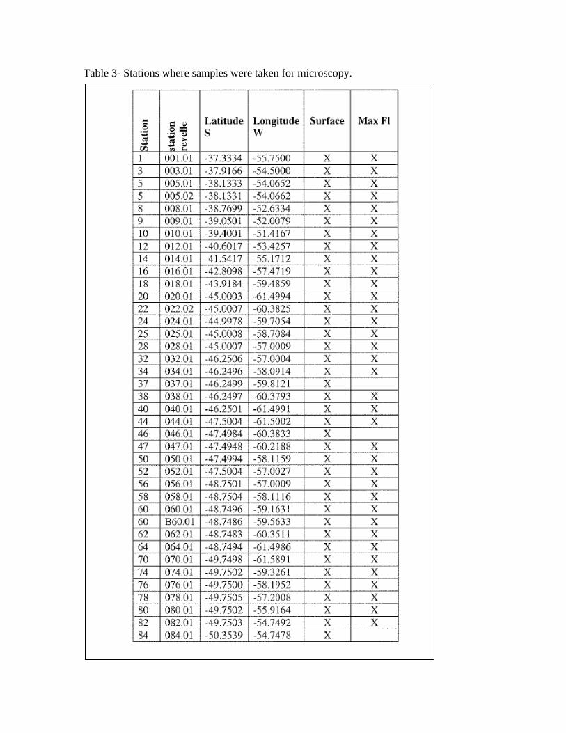
Table 3- Stations where samples were taken for microscopy.

Table 3- continued

References Utermöhl, H. (1958), Zur Vervollkommnung der quantitaiven Phytoplankton-Methodik.

Mitt. int., Ver. theor. angew. Limnol., 9, 1-38

Spatial and Temporal Distribution of Dinoflagellate Bioluminescence

Martha Valiadi , National Oceanography Centre, Southampton, U.K. Charlotte Marcinko, National Oceanography Centre, Southampton, U.K. Dr. Stuart Painter, National Oceanography Centre, Southampton, U.K.

The objectives of this study were to (1) test whether bioluminescent dinoflagellates are present in the Patagonian Shelf; (2) assess their horizontal and vertical distribution in the water column; (3) characterise the taxonomic composition of bioluminescent dinoflagellates; (4) investigate the circadian clock controls of bioluminescence.

To meet these objectives 42 stations were sampled for stimulable bioluminescence and the presence (DNA) and expression (RNA) of the dinoflagellate luciferase gene. At some stations samples for microscopic analysis were also collected. . Where possible, samples were taken at the surface and the chlorophyll maximum.

Measurements were taken using two GLOWtracka bathyphotometer manufactured by the Chelsea Technologies Group. These instruments are designed to provide continuous measurements of stimulable bioluminescence from a constant flow of water. A Bespoke data logging unit then sampled the instrument voltages at up to 1 kHz. The voltage recorded could then be converted into units of photons cm-2 sec-1 using a set calibration equation provided by the manufacturer. All data from the instruments were recorded using Agilent VEE release 8.5 software and stored in a comma-separated numbers (.csv) format.

Discrete bioluminescence measurements were taken for a total of 82 samples over the 42 stations during cruise KNOX22RR (Table 4). Specifically this apparatus was setup in such a way as to maximize the recording of light emission from any bioluminescent dinoflagellates species that may have been present in a 2L water sample. Data were stored using a standard file naming convention as follows ‘nnnnn_ddm.csv’ where ‘nnnnn’ was the 3-digit station number followed by the 2-digit cast number and ‘dd’ was the depth of the sample.

In addition to the discrete instrument a secondary GLOWtracka instrument recorded stimulable bioluminescence continuously during the period 12/05/2008 – 12/31/08 from the filtered underway system. The standard file naming convention for these data were ‘UW_ddmm_partN’ where ‘dd’ was the day of the month, ‘mm’ denoted the month and N was a sequential number for that particular day.

Processing and analysis of all these data will be carried out in the near future using custom based scripts written in MatLab.

Samples for DNA and RNA analysis were collected from the same stations as the bioluminescence measurements unless stated otherwise in Table 4. Seawater was filtered through 12 µm polycarbonate membrane filters which were then stored at -80˚C either dry (DNA) or in RNAlater (RNA). Samples for microscopy were collected from 22

stations and fixed with 2% Lugol’s iodine containing 10% glacial acetic acid. All analysis will be done in Southampton, UK.

Table 4: Overview of stations, Niskin bottles and sample depths for measurements of bioluminescence and collection of samples for molecular/ microscopic analysis. (L) denotes collection of Lugol’s samples for microscopy; (BL only) denotes only bioluminescence measured, no biological sampling; (Bio only) denotes only biological sample collection, no bioluminescence measurement. Station and Cast Reference Number

Bottle Number Sample depths

00101 10 & 4 4 m & 18 m 00301 10 & 5 4 m & 18 m 00501 10 & 5 7 m & 16 m (L) 00701 Underway, 8, & 5 Underway, 22 m & 50 m 00802 Underway & 6 Underway & 63 m 01001 Underway & 9 Underway & 35 m (L) 01002 10 & 3 6 m & 40 m 01301 Underway & 6 Underway & 26 m 01501 Underway & 10 Underway & 20 m 01601 12 & 6 1 m & 19 m (L) 01701 11 & 5 3 m & 19 m (L) 01801 11 & 5 4 m & 51 m (L) 01901 (Bio only) 12 & 35 4m & 35m 02001 11 & 4 4 m & 25 m 02402 12 & 6 5 m & 50 m (L) 03201 11 & 5 4 m & 24 m 03701 Profile Cast no bottle ref 2.4 m 03801 12 & 7 2 m & 25 m (L) 04601 Profile Cast no bottle ref 5.7 m (L) 04701 10 & 6 3 m & 35 m (L) 05202 8 & 4 5 m & 28 m (L) 05601 11 & 4 4 m & 43 m 05801 11 & 5 4 m & 29 m 06001 9 & 4 7 m & 13 m (L) 06601 11 & 5 3 m & 18 m 06801 10 & 4 5 m & 35 m 07001 11 & 4 6 m & 43 m 07201 10 & 5 4 m & 26 m (L) 07301 Profile cast no bottle ref 5 m (L) 07401 11 & 8 4 m & 14 m (L) 07802 6 28 m 08001 11 & 5 4 m & 26 m (L) 08201 10 & 4 5 m & 41 m

08601 11 & 5 8 m & 48 m (L) 09201 (BL only) 11 & 6 3 m & 26 m 10001 10 & 5 5m & 35 m (L) 10201 11 & 5 4 m & 28 m 10801 11 & 5 6 m & 41 m 11601 10 & 4 4 m & 28 m 12201 10 & 4 8 m & 47 m (L) 12801 11 & 5 6 m & 40 m (L) 13401 11 6 m (L) 13601 (BL only) 11 6 m 14201 11 & 5 6 m & 36 m (L)

Education and Outreach Jeff Lawrence, Lowrey School, Tahlequah, OK; Armada teacher The education and outreach component of this work fell into six categories:

1) Interactions with 5th, 6th, 7th, and 8th grade students at Lowrey School, Tahlequah, OK. Mr. Lawrence also interacted with the staff of the ARMADA program at URI (they sponsored his participation). Several of the other ARMADA teachers’ classes also followed along with the journal writings at the ARMADA site. Lastly, pre-service teachers in J. Lawrence’s class at a local college were taught about the science onboard the R/V REVELLE.

2) There were indirect interactions between Mr. Lawrence and his students through the ARMADA site, on a daily basis. They used their laptops to visit the ship’s website and view the cameras onboard the REVELLE as well as get the ship’s location and data for that day. The students posted this on a journal that they kept on their laptops. They also were required to read Mr. Lawrence’s journals, write a paragraph about the daily experience and download photos for a powerpoint presentation that that they created.

3) Life Science Topics covered during the cruise– coccolithophores, phytoplankton,

marine mammals of the S. Atlantic Earth Science Topics covered – ocean density (salinity lab) ocean currents, ocean optics, meteorology (how oceans impact weather around the globe), southern hemisphere anomalies as they relate to weather, satellite imagery, wind currents and Coriolis effect.

4) Using R/V Revelle’s satellite broadband internet access, Mr. Lawrence used Skype (video plus audio) four times over the cruise, and Skype (audio only) another three times. He was able to Skype all four of his classes at least once during the cruise. The face-to-face interaction provided genuine excitement for him and his students. He also was able to post current photos on his own website daily (from the ship).

5) Teaching outcomes: a) Students understand their place in the world and part as

stewards of the earth and ocean environments. b) Students understand how littering can impact ocean marine life in a negative way. c) Students understand that microorganisms such as coccolithophores (phytoplankton) play a vital role in the overall health of the oceans and the planet by sequestering CO2 from the earths atmosphere to the bottom of the oceans. d) Students understand the role the oceans play on weather/climate/and global warming issues of the day. e) Students understand what and how the tools oceanographers use on research vessels are utilized to study the world ocean.

f) Students learn that a better understanding of the world’s oceans, along with research and technology, may help to minimize the cumulative effects of anthropogenic injections of CO2.

6) URL’s for R/V Revelle education and outreach: Readers can read his journals for

that trip at: http://teacheratsea.noaa.gov/2006/lawrence/index.html Also the ARMADA journals for the COPAS ‘08 trip are at: http://www.armadaproject.org/journals/2008-2009/lawrence/12-2.htmHis homepage also has some information about the trip and other activities at: http://web.me.com/jefflawrence62/Site/Welcome.htmlHe continues to look for new ideas to bring into the classroom and provide his students with information and opportunities not normally available to land-locked students. Being land locked does not allow much education in the ocean sciences. Indeed, earth sciences often represent a small subset of curriculum science in most states and they should be a primary focus for students to ensure a better future for the planet. Mr. Lawrence’s students were able to participate along on this cruise due to the special nature, timing, and availability of technology onboard R/V Revelle and at his school. This combination of technology provided a truly unique experience for him and his students, and other educators who visited his site. He also has used this experience at a Teacher conference meeting (NOMSTA) to make teachers aware of climate change issues in our oceans and how to participate in such programs as ARMADA and NOAA’s Teacher at Sea. His college teacher students at NSU also benefitted from the experience (he teaches pre-service teachers how to teach inquiry science in the classroom and have given several talks and an overview of the science that he participated in while at sea). The goal of this work is to instill a vision to pursue ocean sciences in their future classrooms in Oklahoma or elsewhere.

Acknowledgements The captain of R/V Revelle (Capt. Tom Desjardins), officers (Chief Mate, Muray Stein, Second Mate, Heather Galiher and Third Mate, Chris Sheridan), engine and deck crews are to be commended for making all of this work possible. Their professionalism and sea handling were exemplary. Matt Durham (SIO, STS), was the resident technician for this trip who provided expert logistical support before, during and after the trip. He was ably helped by Rob Palomares (SIO STS), Bud Hale (SIO, computing), Dan Yang (SIO, computing) and Dan Schuller (SIO, chemistry). Moreover, we would like to thank staff at the Scripps Ship operations department for excellent logistical support (Capt. Tom Althouse, Rose Dufour, Elizabeth Brenner, Graziella Bruni, Woody Sutherland, Kristen Sanborn, and many others too numerous to mention). Gary Lain and Dave Skydel helped with isotope details. Dr. Andrew Dickson and the SIO radioisotope committee also helped expedite the radioisotope work. Jeff Brown (Bigelow RSO) helped with the shipping and paperwork for the isotopes from Bigelow Laboratory. Capt. Juan Abelleyara (Servicio de Hidrografia Naval Buenos Aires, Argentina) served as Argentine observer on this cruise. He was on deck for each and every cast of his watch, helping to deploy and recover the CTD/Rosette. I would also like to thank the personnel at the U.S. State Department and embassies of Argentina and the United Kingdom for their help in processing our request to work in foreign waters. The ship time and much of the research was supported by the National Science Foundation (OCE-0728582 to WMB). Secondary support for WMB came from NASA (NNX08AJ88A). Support for the participation of J. Lawrence on the cruise came from the NSF Armada Program (grant to S. Hickox, Univ. Rhode Island). Several aspects of the research carried out by the UK’s NOCS team were supported by the DSTL under grant no: JGS 1166.