#ss

high-

fidelity

circuit design

norman h.crowhursl

and

george fletcher cooper

published by gernsback library, inc.

First Printing — April, 1956.

Second Printing — April, 1957.

© 1956 Gernsback Library, Inc.

All rights reserved under Universal,

International, and Pan-American

Copyright Conventions.

Library of Congress Catalog Card No. 55-11190

jacket design by muneef alwan

chapter

Part 1 — Feedback

page

chapter page

introduction

Many books have been published on the various aspects of

audio that can broadly be divided into two groups: the

“theoretical” group, which undoubtedly give all the theory any-

one needs, provided he has sufficient knowledge of advancedmathematics to be able to apply it; and the “practical” group,

which tell the reader, step by step, how to make some particular

piece of equipment. What has been lacking in the literature is

some information in a form that will enable the man with only

the most elementary knowledge of mathematics to produce his

own design and make it work.

With the objective of filling in this gap, we have written various

articles that have appeared in Radio-Electronics magazine. Andthe correspondence we have received assures us that we haveachieved our objective in this. In fact, many people find the only

complaint is the inconvenience of having numerous copies of

Radio-Electronics strewn about the place for easy reference!

For this reason the Gernsback Library undertook the assembly

of this material into book form. But a number of separate maga-zine articles do not too readily go together to make the best book,

just like that. The result is apt to be rather a mass of bits andpieces. So the authors’ help was called upon, and the original

articles have been considerably edited and rewritten. In several

places additional material has been added, in the interest of over-

all clarity, and to fill in some gaps that naturally result from pre-

paring a book in this way. But now that we have finished the workwe feel confident in offering it to the reader as a real primer ondesigning the best in audio.

Often people ask where we get the ideas for articles. We feel this

introduction is a good opportunity to give the answer to this ques-

tion, as credit to whom credit is due. Practically all the subjects

for our articles arise from questions various people have asked,

and the discussions that have followed. To be able to explain a

5

subject successfully, it is necessary not only to understand it prop-

erly one’s self, but also to understand the obstacles that make it

difficult for others to grasp. It is odd how obstacles in the attain-

ment of knowledge seem insurmountable as we approach them,

but having passed them, they seem to vanish, and we find it diffi-

cult to realize the obstacle ever existed. This is why questions

from people seeking knowledge, and the discussions that ensue,

are invaluable in providing material for this kind of presentation.

Knowing that many look in the introduction of a book to find

out for whom it is written, we should answer that. While we haveavoided using expressions that would put it over the heads of the

many enthusiasts who do not possess very much theoretical knowl-

edge, we are also confident that much of its contents will prove

helpful to many who have more advanced training, but who havefailed to visualize adequately some of the problems they en-

counter, largely due to the vagueness of the “classical” approach.

As a “primer” to read, it will give a sound basic knowledge of the

subject, after which it will serve for years as an invaluable refer-

ence book. We make no apology for such a claim — we use our ownwritings for reference. It’s so much easier than trying to memorizeit all!

Norman H. Crowhurst

George Fletcher Cooper

6

chapter

1

feedback effects

Boil water and butter together. Add flavor. Cook till it forms a

ball. Season, and beat in an egg.

This is not a book on cookery, nor is it one of those with a cook-

book approach on how to build the perfect amplifier. “Take a ripe

output transformer, about four pounds,” he says; "two large well-

matched tubes and an assortment of smaller tubes, capacitors andresistors. Connect as shown. Add feedback to taste." The trouble

is, that the amplifier described this way is never just what youwant, and nothing in the book tells how you can alter it without

ruining the performance completely. Consequently, when you or

your employer needs an amplifier, it has to be designed fromscratch. Amplifiers without feedback are no problem, but the ad-

dition of a reasonable amount of feedback to an amplifier with

more than two stages usually leads to instability unless the circuit

is carefully designed.

To begin with, why do we want to use negative feedback in am-plifiers at all? There are four reasons which assume different orders

of importance, depending upon the function of the amplifier. If

the amplifier is part of an a.c. voltmeter, the gain must be con-

stant in spite of changes in supply voltages and aging of tubes. Avoltmeter with a drift of 10% would be a thorough nuisance in

any laboratory. After all, unless you are a magician, you must trust

something. By using negative feedback, the overall gain can be

made almost independent of the internal gain of the amplifier;

once it is adjusted, the gain will be the same even if the tubes

7

are changed or the line voltage drops 5% . If the gain is independ-

ent of the plate supply voltage, ripple caused by inadequate filter-

ing will not modulate the signal. This aspect is especially impor-

tant for ordinary program amplifiers.

The reasons for using feedback are also important in audio. Byusing negative feedback we can flatten the frequency response, and

reduce the harmonic and intermodulation distortion. It can also

be used to modify effective input or output impedances.

Feedback improves response

Let us first consider how negative feedback helps keep the gain

of an amplifier constant. A particular amplifier has a gain of 80

db 1; an input of 1 mv between the first grid and cathode gives an

output of 10 volts. When the input and output impedances of an

amplifier are not equal:

db gain (or loss) = 20 log _p io log + 10 log-^- (1)

where Ei and E2 are the input and output voltages; and Z 2 rep-

resent the input and output impedances respectively; kj. and k2 are

the power factors of the input and output impedances. However,if input and output impedances are identical (as in our example)

,

the formula for db gain or loss of an amplifier is simplified to2:

db gain (or loss) = 20 log (2)e-i

With an input of 1 mv (.001 volt) and an output of 10 volts,

db gain = 20 log = 20 log 10,000 = 20 X 4 = 80 db

We now connect across the output a network which gives exact-

ly 1/1,000 of the output voltage. We can readily calculate the loss

in this network. Since the output voltage is 10 volts, the voltage

across the output will be 10 millivolts. Using formula (2) :

db loss = 20 log^= 20 logH= 20 log 1,000 = 20 X 3 = 60 db

1 These are not true decibels, as the impedances are not necessarily the same. "Thequestion is,” said Alice, "whether you can make words mean different things."

“The question is,” said Humpty Dumpty, "which is to be master—that’s all."

(Through the Looking Glass— Lewis Carroll.)

2 Throughout this work, all log formulas are to the base 10.

8

Thus our network has a loss of 60 db. When the input to the am-plifier is 1 mv, the amplifier output is 10 volts and the network

output is 10 mv.

The output of this network is now connected in series with the

input, so that the voltage appearing between grid and cathode of

the first tube is the difference between the applied input between

grid and ground and the voltage fed back through the network.

Working backward, we see that if the output is to remain at 10

volts with a feedback voltage of 10 mv, then we must increase our

input to 11 mv (1 mv for input signal and 10 mv to overcome the

effect of the feedback voltage on the input voltage). The overall

gain is now 10 v/11 mv, which equals 59.17 db, since:

db gain = 20 log~

= 20 logJjL = 20 log 909

log 909 = 2.9586

db gain = 20 X 2.9586 = 59.17 db

Since our amplifier, without feedback, originally had a gain of

80 db and with feedback has had its gain reduced by a little morethan 20 db, let us see what advantage we secure by this sacrifice of

gain.

Suppose now that we make some change in the amplifier, so that

for 1 mv between grid and cathode we obtain 20 volts out. Thevoltage feedback will be 20 mv, so that this 20-volt output requires

an input of 21 mv and the gain is 20 v/21 mv=59.58 db. Althoughthe internal gain has been doubled (6-db increase), the overall

gain has increased only by about 5%, or 0.41 db.

This example shows immediately how negative feedback im-

proves the performance of a voltmeter amplifier. By using morefeedback, even greater constancy of gain can be obtained. A little

thought will show that the other properties of negative feedback

can also be obtained in this example. Suppose that the change of

gain was the result of changing the test frequency. For example,

the gain might increase by 6 db when the frequency is increased

from 50 to 400 c.p.s. The feedback keeps the gain the same within

0.4 db for this change of frequency.

The reduction in distortion is not as simple. In the normalworking range of the amplifier the gain is not quite constant at all

points in the voltage wave. This can be seen by looking at a graph

9

showing mutual conductance plotted against grid bias. These vari-

ations in gain during a single cycle cause distortion; but obviously

since negative feedback keeps the gain nearly constant, the distor-

tion must also be reduced.

At this point the reader is warned not to open his amplifier to

connect a simple potential divider from loudspeaker terminals to

input grid. By a well-known law of Nature (the law of the cussed-

ness of inanimate things) you will be certain to add positive feed-

back and will produce an excellent oscillator. Relax in your arm-

chair and continue to read this book.

Oscillation troubles

The problem which really causes trouble in negative-feedback

amplifiers is oscillation of the extremes of the frequency range.

When feedback is applied to an amplifier with more than one

INPUT e2|

outputFig. 101. Basic feedback-amplifiercircuit. The feedback networkfeeds part of the output signal

back to the input. When thefeedback is negative, the voltage

fed back to the input is out ofphase with the original input

signal.

stage, oscillations may occur either at very low or very high fre-

quencies. Fairly typical values would be 2 c.p.s. and 30 kc. It is dif-

ficult to detect the high-frequency oscillations just by looking. Theamplifier appears to have no gain but lots of distortion. With anoscilloscope, of course, the trouble is easily found. There are nocertain cures which can be applied to all amplifiers: one man’smeat is another’s poison. In our view, the only safe way to proceedis to draw the amplitude and phase responses (later in this book,it will be shown how this can be done easily).

A little mathematics

Before discussing the specific problems of design, let us look at

some of the basic mathematics. The generalized circuit of a feed-

back amplifier is shown in Fig. 101. It consists of an amplifier hav-

ing a gain of A and a feedback network having a gain (actually a

small fraction) of /?. The two equations are:

17= A and qr~= P (3)

Suppose we call the gain of the amplifier including feedback A'

10

to distinguish it from the gain A of the amplifier without feed-

back. The overall gain is:

Since the feedback is negative the feedback voltage must sub-

tract from the input voltage to give the voltage E, actually applied

to the grid, or:

E, = E„ - E3 (5)

For convenience we can rearrange this equation to read:

E<> = Ej. + E3 (6)

Suppose we substitute (Ei + E3)for E0 in equation (4) (which

we can easily do because the two quantities are equal to each

other). We then get:

A' = E*

Ei + E3(7)

So far we see that nothing spectacular has happened, but fromequation (3) we know:

We can now put this value for Ei into equation (7) and we will

get

A' = E2

E2 4- E,E3(8)

Combining the denominator terms on the right-hand side, wehave:

A - E°-e2 + e3a

AClearing the division of fractions, we get

E2A_e2 + e3a

We know from equation (3) that E3 = ]3E2 . We can substitute

this value for E3 and arrive at a gain value of:

A' - E*A- E2 + /?E2A (9)

11

We can now factor the denominator:

A' -- E2(l + Afl)

Cancelling E2 in numerator and denominator, the gain of anamplifier with feedback is seen to be:

A' — -~1 + A/?

(10)

The term A/3 in this equation will be called loop gain although

some other authors have referred to it as the feedback factor or

feedback ratio. One additional point to note here is our usage of

A/ (1 + A/3) as representing negative feedback gain. This form is

based on the algebraic rather than on the magnitude value of ft.

In some engineering texts, the form A/ (l-A/3) is used, assuming of

course that /3 itself is negative for negative feedback. This formresolves itself algebraically to:

A/ A A“

1 - <-/»A ~ 1 + A/3

In terms of numbers we can make this factor have practically

any value we want by adjusting the gain of the amplifier and the

amount of feedback voltage. Suppose we make Aft much larger

than 1. In this case, the quantity (1 -f- A/3) in equation (10) is very

nearly equal to just A/3, and for all practical purposes we can write

equation (10) as:

and the gain of the amplifier with feedback is:

(H)

Since the A drops out, the gain A' of the amplifier with feedback

is independent of the gain without feedback as long as the loop

gain A/3 is fairly large as compared to 1. To meet this condition,

A/3 would usually have to have a value of at least 1 0.

Equation (12) is of interest in that it shows directly that the gain

of an amplifier is inversely proportional to the amount of feed-

back and, as the amount of feedback is increased, the gain of the

amplifier is reduced.

Earlier in this chapter the formula for the gain of an amplifier

in db was given as:

Eodb gain (or loss) = 20 log -g=-

12

Using this formula, we can obtain an expression for a feedback

amplifier in decibels, making use of formula (10);

20 log A' — 20 log A - 20 log (1 + Aj8) (13)

Without feedback the gain in decibels is 20 log A. The effect of

the feedback is to reduce the gain by 20 log (1 + A/3) decibels.

This latter term is correctly called the feedback factor.

Effects of phase shift

So far we have assumed that ft and A are just ordinary num-bers. If the feedback network is just a couple of resistors, this is all

right as far as /? is concerned. However, amplifier gain A has

a phase angle which depends on the interstage coupling networks

and transformers if any are used.

Fig. 102. A typical R-C network.

Since the capacitor (C) blocks the

passage of the B-supply voltage into

the grid circuit of the second stage,

only the a.c. signal component fromthe first stage is coupled into thegrid circuit, and appears across re-

Fig. 102 shows a typical resistance-capacitance coupling circuit.

At some frequency the reactance of C will be equal to the resist-

ance R. At this frequency the phase shift between the plate of the

first tube and the grid of the second tube is 45° and the response

has fallen by 3 db. At still lower frequencies the phase shift gets

larger until it approaches 90°.

To understand this, let us assume a condition such that R = Xc .

However,

Xc = o (14)

and since (at a particular frequency), R = Xc , then

R - 1R “ 2^fC (15)

An elementary rule in arithmetic is that a number multiplied

by its reciprocal is equal to I. Although this sounds formidable,

it simply means that a number such as 6, when multiplied by its

reciprocal, 1/6, is equal to 1 (6 X 1/6=1). We can apply the

same reasoning to Xc and R since we have deliberately chosen a

frequency at which these two are equal. Thus we have:

1

Xc

R = 1 (16)

13

Another basic rule in arithmetic states that if numbers are

equal, then their reciprocals are also equal. This simply means

that if 6 = 6, then 1/6 = 1/6. Using this principle we can change

formula (16) to read:

i- =\

= 2^C (17)

2ACNow by substituting the right-hand member of this equation in

place of 1/XC in equation (17) , we will have:

27rfCR =1 (18)

When the frequency makes R = Xc , then the voltage across the

capacitor and across the resistor will be equal since the ohmicvalues of the two components are identical.

Now let us take a condition in which

2^fCR > 1 or f >

Since the frequency has increased, the capacitive reactance has

gone down accordingly; the signal voltage across the capacitor is

smaller, while the signal voltage appearing at the input of the

amplifier stage (across R) has become larger.

The final condition, of course, is one in which

2;ifCR < 1 or f < ^-L_

Since this represents a decrease in frequency, the capacitive re-

actance is increased; and the signal voltage across the capacitor is

also increased, while the useful driving voltage (signal voltage

across R) is cut down. Under these conditions, the phase angle

approaches 90° and the volume decreases.

In a three-stage amplifier there will be two coupling circuits of

this kind plus a third to keep the plate d.c. from the feedback

network. If the C-R products of these three networks are equal,

each will have a phase shift of 60° at some frequency and the total

phase shift will be 180°. Where a C-R circuit has a phase shift of

60°, it also attenuates the amplitude to one-half, or 6 db. Thus,three such circuits will attenuate to \/% X X J/2 = Vs or 18 db.

The correct value for the gain at this frequency is then not

A but -1/gA. The gain with feedback is then equal to:

A' -~1 - VsA

P

A but —i/s A. The gain with feedback is then equal to:

14

(19)

this equation is equal to 0 and the gain is infinite. Obviously this

will not do because we want an amplifier, not an oscillator, so wemust arrange for i/^A/3 to be less than 1 at the frequency where

the phase shift is 180°. For to be less than 1, A/3 must be

less than 8, or 1 -j- Aft less than 9. This means that a three-stage

amplifier using equal C-R couplings must use less than 20 log 9 =19.08 db feedback or it will oscillate. By using unequal values of

C-R, this limit can be raised as we shall learn later.

Up to this point we have just considered two very special con-

ditions in which the output voltage of an amplifier is either direct-

ly in phase with the input signal or completely out of phase with

it. The phase of the output voltage of an amplifier without feed-

back (compared to the incoming signal) will vary between these

two extremes at different frequencies, depending upon the value

and type of the coupling components. If we have an amplifier

using negative feedback with large phase shift at some frequency,

then there will be an equally large shift in the phase of the feed-

back voltage, thus reducing the effectiveness of the feedback at

this frequency. For this reason the gain can increase, producing a

bump in the frequency response at one end or the other or per-

haps at both ends. If the amplifier is well designed—that is to say,

if the amount of feedback is properly controlled—these bumpswill not appear. A low-frequency bump at 60 c.p.s. is obviously

not desirable; and if the amplifier is used with a phono pickup, a

low-frequency bump can be a nuisance. High-frequency bumpsare equally bad since they increase the noise level.

Feedback design

The designer of an amplifier may often be confronted with the

problem of knowing how much the gain of his amplifier could

change for a given amount of feedback. Alternatively, he may wish

to keep the change of gain of his amplifier within prescribed limits

and will want to know just how much feedback is necessary to

achieve this. Actually, these two problems are identical. In each

case the designer has a problem involving small changes.

Since differentiation is the technique by which we can solve

problems dealing with rate of change, we can differentiate equa-

tion (10) and arrive at an important and useful tool. First, let us

repeat equation (10):

1 + A/3

15

We can rearrange this equation to read:

By differentiating this equation we then get:

dA' dA w 1

~Ar~ "X X

1 + Ap (21

)

In this form the terms dA' and dA represent moderate changes

of gain in an amplifier with and without feedback. Rate in this

case does not involve the idea of time. If variations of supply volt-

ages or circuit components produce a change in the gain of the

amplifier without feedback (dA), then this change will be a frac-

tion (dA/A) of the total gain A. The change of gain with feedback

is dA'/A'. In other words, any variations in gain of the amplifier

will be reduced by the fraction 1/(1 —{— A/?) when the circuit has

a feedback factor of A/3.

Solution of a sample problem

Equation (21) is very useful for designing amplifiers to rigid

specifications. Let us assume that we want an amplifier with feed-

back to have a gain of 1,000, with a maximum possible tolerance

of gain not to exceed ±2%. A deviation of 2% means that 1 volt

could change to 1.02 volt. To numerically express this change in

db, we take:

20 log = 20 log 1.02 = 0.17 db

The gain of the amplifier in db is then:

db gain = 20 log^5= 20 log 1,000 = 20 X 3 = 60 db (±0.17 db)

Suppose that this particular amplifier, without feedback, can in-

crease its gain by 50%. In terms of db, this would be a change in

gain of 3.52 db. To a person listening to such an amplifier, this

change would be barely noticeable. However, for voltmeter ampli-

fiers, modulators and high-fidelity amplifiers this change mightvery well be considered intolerable.

In this problem, the change of gain with feedback is 2% , or .02.

Thus we get:

16

The change of gain without feedback is 50%, or 0.5, and so wehave:

If we now substitute these values in equation (21), we will have:

.02 = (0.5)1

1 + A/?

' “1 + A0

Transposing, we get

0 5

1 + A/? = ig = 25

Now A' = 1,000 and we can find the value of A from the equation:

,yA

1 + A/?

or

A = A'(l + AjB)

Substituting our values in this equation, we have:

A = 1,000 x 25 = 25,000, or 87.96 db

Our amplifier would require an initial gain (without feedback)

of 25,000, or 87.96 db. Our feedback factor would be 25. Because

of this feedback, the gain of the amplifier would be reduced to

1,000 (60 db) while the change in gain of the amplifier would be

down to ±0.17 db.

Most people use negative feedback, not to provide constant

gain, but to reduce the distortion. Usually most of the distortion

originates in the output stage. For this reason, the feedback is

sometimes applied only to the output stage. This is not as useful

as it appears, for the previous stage must now provide much more

drive and usually begins to make a substantial contribution to the

distortion.

In subsequent chapters, charts will be given so that you can cal-

culate easily the phase and amplitude response and, hence, the

stability conditions of amplifier circuits.

Gain without feedback

Now that we have examined the basic principles of negative-

feedback amplifier design, we can readily see that the quantity of

17

key importance is the feedback factor (1 -j- A/3). Expressing the

feedback factor in db, it becomes:

F = 20 log (1 + A/?) (22)

If Ap is fairly large, this is almost identical to the condition

where there is no phase to consider with the loop gain. Thus:

F = 20 log A/3 (23)

This of course can be factored to:

F = 20 log A-f- 20 log p

Most of our attention has to be focused upon the first term

(20 log A), which is the gain of our amplifier without feedback,

since /3 is relatively simple to handle.

The first thing to do is decide what you want. This may sound

platitudinous, but even professional designers sometimes try to

produce amplifiers which are not possible. We have discussed

some of these basic design problems. For example, if a 6AQ5 beampower output tube is to give 4.5 watts, the distortion without feed-

back will be, according to the maker’s specifications, 8%. To get

only 1 %, it is necessary to use about 20 db of feedback. The mu-tual conductance is 4,100 pmhos, the optimum load 5,000 ohms.

Therefore the gain will be about 20, or 26 db. The input stages

of the amplifier must therefore provide most of the total gain weneed.

If we want, say, 50 db all together, the gain without feedback

must be 70 db. Since the 6AQ5 will supply 26 db, the earlier stages

must have 44-db gain. This is an awkward example because 44 dbis just about on the limit for a single high-gain pentode. Weshould have to look closely to decide whether to use two stages

before the 6AQ5 and have the advantage of the extra feedback

or risk the distortion rising to perhaps 2% at full output.

Where to apply feedback

In this preliminary design, we must decide where the negative

feedback is to be applied. Voltage feedback can be applied either

to the grid or the cathode of the input stage in the ways shown in

Fig. 103. The second way (Fig. 103-b) is useful only for feedback

around a single stage because the resistances in the feedback con-

nection must be very high and stray capacitances then become im-

portant. The method of Fig. 103-a has the disadvantage that the

secondary of the transformer is not directly grounded; but as the

resistance R is usually only about 100 ohms, this is not serious.

18

This method allows the cathode to be bypassed, thus increasing

A and therefore A[3, the feedback factor. The cathode R-C circuit

is sometimes useful for increasing the stability margin. Themethod of 1 03-c is simple if the loss of gain due to the unbypassed

cathode can be allowed.

4 i c

Fig. 103. Three common ways of applying voltage feedback to an

amplifier input.

If the feedback voltage cannot be taken from a transformer,

there is no way to reverse its polarity. In that case Fig. 103-a or-b

must be used with an odd number of tubes and 103-c with an even

number. Otherwise the feedback will be positive. This assumes

that the output is taken from the plate and not from a cathode

.load. When the feedback is taken from the output side of an out-

put transformer, circuit 103-a is the best because there is no d.c.

in the feedback circuit and no capacitors are needed. If 103-c is

used, a blocking capacitor must be used to keep the cathode volt-

age off the output line. This capacitor usually must be very large

because of the low impedances normally used in this type of cir-

cuit. Some output transformers have separate windings for feed-

back.

Safety margins

An amplifier will be unstable if the total or sum of the phase

shifts through it reaches 180°, while at the same time the value of

the loop gain (A/8) is equal to 1. Let us look at the typical ampli-

fier response shown in Fig. 104, and analyze it in terms of ampli-

tude characteristics and phase response before continuing ourdiscussions of phase shift.

At frequencies between 256 and 2,048 c.p.s., the amplitude char-

acteristic is very close to flat and the phase response is practically

zero. This means that the coupling capacitors and transformer

inductance (if a transformer is used) have negligible effects, the

15

coupling capacitor reactance is very small compared with the grid

resistor and the primary inductance of the transformer has a re-

actance very high compared to the plate load impedance. It also

means that the various stray capacitances that cause loss at the high

frequencies still have reactances that do not appreciably shunt the

circuit impedances.

At frequencies from 128 c.p.s. downward, the amplitude re-

sponse drops off and the phase response shows advance angle. This

is due to the rising series reactance of the coupling capacitors. In

the interstage couplings a progressively larger proportion of the

voltage developed at the plate of the previous stage gets dropped

across the reactance of the capacitor and a progressively smaller

proportion reaches the grid resistor of the following stage. At the

same time, there is a 90° phase difference between the voltage

dropped across the coupling capacitor reactance and that across

the grid resistor. The voltage across the capacitor lags behind that

across the resistor. When most of the voltage developed is dropped

across the capacitor, the two will then be almost in phase, and the

voltage across the grid resistor must be almost 90° out of phase

with the input voltage. It is the grid resistor voltage which is

passed on for further amplification. If the voltage across the capaci-

tor lags behind the voltage across the resistor, then, conversely, the

voltage across the resistor must lead, or be ahead of, the voltage

across the capacitor. This means that the output voltage is actually

ahead of the input voltage under this condition. It is indicated in

Fig. 104 by showing the angles in negative degrees. The “wavi-

ness” of the characteristic is a result of the irregularity with which

the different R-C values of the coupling circuits take effect.

At frequencies above about 4,096 c.p.s., the amplitude response

again departs from level and eventually rolls off, and the phase

curve goes into positive angles, representing phase lag or delay.

At these frequencies the output is behind the input. This devia-

tion is caused by the various stray capacitance effects. Grid to

ground, plate to ground and stray wiring capacitance all con-

tribute to this effect. The slight rise before falling off may be

caused by interaction between the leakage inductance of the out-

put transformer and its capacitance, forming a tendency to reson-

ate. (Leakage inductance should not be confused with primary

inductance. It is like an inductance in series between source andload, causes a loss of high frequencies rather than low, except

where it resonates with some capacitance elsewhere in the circuit).

20

Instead of using 180° as the phase limit, we shall use 150° to

give us a safety or phase margin of 30°. At some low frequency the

phase shift between the input signal voltage and the output signal

voltage will reach 150° and the gain will be less. If, as before, werepresent the gain of an amplifier without feedback as A, then the

gain of the amplifier at the low-frequency end will be less than A.

To meet the conditions of stability at the low-frequency end

the loop gain (A/3) should be no greater than the amount by

which the midband gain (without feedback) is reduced at the

FREQ IN CPS

Fig. 104. Typical amplitude and phase characteristics of an audio amplifier.

frequency where the phase shift is 150°. In turn, the limit on the

size of the feedback factor is determined by the amount of ampli-

fication decrease at the low-frequency end (using mid-frequency

as a reference) in an amplifier without feedback. To understand

this more clearly, refer to Fig. 104 in w'hicli the amount of drop in

gain at the 150° point is show'll by the length of vertical line A.

We can reduce the gain by this amount when we apply feedback.

If we use more feedback than this, A/3 becomes greater than unity

at the 150° point and the circuit has insufficient margin of stability.

21

Exactly the same conditions apply to the high-frequency end.

Here we also use the 30° phase margin. In Fig. 104, the length of

vertical line C is the limit we should observe to keep the amplifier

stable at the high-frequency end.

At more extreme high and low frequencies, the phase shift will

reach 180°. At these points the difference between the actual feed-

back and the amount the response without feedback has fallen is

called the gain margin. These are indicated by B and D in the

response curve. The phase and gain margins are merely safety fac-

tors chosen so that the amplifier will not be running too close to

its instability limits. A typical value for the gain margin is 10 db.

The phase shift can be allowed to be more than 150° as long

as it dips back to that value. This is shown in Fig. 105. Point B onthat curve is the one to use, and not A. This is true even if the

I

i

Fig. 105 . Curve showing how the phase shift may go beyondthe phase margin.

curve dips below the 180° line at C. In this case, however, the

amplifier is only conditionally stable and might oscillate whenfirst turned on. It is best to avoid such a condition because it is

hard to handle. We will return to this question of margins later.

Calculated response

We are now faced with the problem of calculating the response

of the amplifier. Let us first concentrate on the low-frequency end.

Two things cause the low-frequency response to drop off. Oneis the reactance of plate, screen and cathode decoupling capacitors;

the other is the reactance of the interstage coupling circuits. Theeffect of decoupling is usually considered a refinement and will

be considered separately.

IBB IB ing SB!SEEnBM ns IBB

SB!IB in

UfMMB

SB!j|VMmm\ B Ifll IBB

SiimIBS

BB IBSIBB

I 2 4 8 16 32 64 128 256 512 1024 2048 4096 8192 16,384

FHEQ-CPS

22

At low frequencies an interstage coupling can be reduced to

an equivalent as shown in the series of diagrams of Fig. 106-a.

First the plate resistance of the tube is considered in parallel with

the plate coupling resistor. Then, because the capacitor is the

only frequency discriminating part of the circuit and the resist-

ance parts can be considered a simple potentiometer following

f

Fig. 106. At (a) is shown an interstage coupling reduced to its equiva-lent circuit where capacitor C is the only frequency discriminating

part of the circuit. At (b) is the equivalent circuit when a transformeror choke is used where its inductance contributes to the low fre-

quency response.

the capacitor, which has no effect on low frequencies, it appears

that the turnover frequency (<o0) occurs where the reactance of the

coupling capacitor is equal to the parallel combination of Rp andRc in series with Rg, or

<°° =7 \

(24)

Where a transformer or choke is used, its inductance also con-

tributes to the low-frequency response, and the equivalent can be

reduced as shown in the series of diagrams at Fig. 106-b. First, the

load impedance connected to the secondary of the transformer is

multiplied by the square of transformer stepdown ratio. (If the

transformer is an interstage stepup, the secondary resistance is

divided by the square of the ratio). The resultant primary load

is combined in parallel with the plate resistance of the tube, and

23

the turnover point occurs where the reactance of the inductance

is equal to this resistance combination, or:

RPN 2RL

Rp + N 2Rl

Ln

RpN2RlLp

Rp + N2Rl(25)

Fig. 107 shows the curve produced by any single reactance caus-

ing a low-frequency rolloff. This curve is normalized, by which

Fig. 107. The amplitude characteristic of amplifier coupling circuits. This curve is

used to make the template discussed in the text.

we mean that a reference frequency has been chosen to make it

universally applicable. In this case, the frequency marked as 1

is the frequency at which the reactance of C or I. is equal to the

appropriate resistance value, or to0 of equations (24) and (25).

The numbers on the frequency axis of Fig. 107 are the ratio of

the frequency at that point to the normalized frequency, or to/co0

where to = 2A and <o0 is the turnover frequency.

You will notice that this curve is drawn on linear scales rather

than the logarithmic one usually used for frequency response

curves. Various makers use different spacing for their logarithmic

paper, and, since we are going to make a template from this curve,

we could use the template only with the same make of paper if

24

we use log paper. If you transfer this curve to centimeter-square

or inch-square paper, you won’t have this trouble. Besides, linear

paper is much cheaper than log paper and an amplifier design

may use up quite a lot of paper.

To make the template (Fig. 107), trace and then paste the

curve to a stiff sheet of paper. Draw in the numbers indicating

frequency on the template, which is now the upper part of the

normalized response curve cut out.

An alternative method of making the template is to copy the

curve onto centimeter or half-inch square paper. Paste this to a

sheet of -jV-inch celluloid and scratch through the 0 db, w/to0 —1 line, and the curve itself. Now fill the scratches with black wax(boot blacking) and cut out. You can now wash off the paper,

since the template has now been etched into the celluloid.

Fig. 108 . A simplified amplifier circuit to illustrate the

interstage coupling.

A sample problem

Suppose we wish to draw the response curve of the amplifier

shown in Fig. 108. The first step is to prepare a sheet of graph

paper with the same size squares as are used on the template.

Draw in the decibel scale the same as in Fig. 107 and put in a fre-

quency (to) scale. Notice that equal intervals on the frequency

scale represent a doubling of frequency.

Now we determine the three values of w0 for the three coupling

circuits. Rp + RL is the resistive load on the plate of the output

stage. For the first coupling circuit:

1

Wl - (R1)(C1)

6)1 =(10

5)(.01 X KF6

)

= IF5" = 1,000

In this case the coupling resistor and plate resistance in parallel

will be less than 10,000 ohms, so the error incurred in leaving

25

them out of the calculation will be less than the tolerance on resis-

tor or capacitor values.

Since co = 2irf, we can easily divide 1,000 by 2n and arrive at

a frequency of 160 c.p.s. At this frequency, the signal voltage

across Cl is equal to the signal voltage across Rl, and the gain

Fig. 109. Graph showing the amplitude response of each of three coupling circuits

and the final curve (I -j- 2 -j- S) which results when the three are added.

is down by 3 db, for this particular circuit. We must now take

into consideration the effect on the response curve of the remain-

ing coupling circuits:

= 100 (16 c.p.s.)' ~ (R2)(C2)

and using the same approximation we will find

1.4 X 5 X 10® 7 X Iff*

(1.4 + 5) X lO3 x 9 6.4m 125 (19.9 C.p.s.)

26

First place the template on the paper so that the reference line

is at <0i = 1,000 and trace the curve. Move the template sideways

so the reference line is opposite w2 = 100, and trace another curve.

Then place the reference line opposite <o3 = 125 and trace the

third curve. Now you should have three curves like 1, 2 and 3 on

a graph that looks like Fig. 109. Each of these curves shows the low-

frequency attenuation of the coupling circuit in question.

To get the overall response add the attenuation of these three

curves. At some frequency, measure the distance from the 0-db

line to curve 2 (a pair of dividers or a compass is handy for this).

Fig. 110. The phase curve of the coupling circuits (Fig. 109). This curve is also

normalized.

Then, below curve 1 mark a point equal to this distance. On our

curves for example, at 50 cycles we mark off distance A to curve

2, then mark off this same distance A below curve 1. If you do this

for a number of points, you will have points on curve 1 plus curve

2. In exactly the same way measure the distance from the zero line

to curve 3 at the same frequency points used for curves 1 and 2

and mark off this distance below the new curve (1 -(- 2). Draw a

continuous line between these points and you have the sum of the

three curves—the overall response curve of the amplifier. Or, you

can put a straight edge against the left hand margin of the tem-

plate, and ride its parallel to the db axis.

Interpreting the phase-shift curve

We can glean a few bits of interesting information from Fig.

110. The maximum transfer of signal voltage through a coupling

circuit takes place when the circuit is purely resistive and has a

0° phase shift. The introduction of a phase shift means a loss in

27

gain since less useful signal voltage is developed across the grid

resistor. The greater the phase shift, the greater the voltage de

crease across the grid resistor until at 90° we should theoretically

get no transfer of signal through the coupling circuit from one

stage to the next so that the attenuation of the signal across the

grid resistor should be infinite, resulting in zero output from the

speaker. Each coupling circuit conspires to give us a phase shift

as well as a signal loss. The effect of successive stages is cumulative

Fig. 111. Phase shift curve of the amplifier of Fig. 108. Curve2 represents the shift of the circuit if the amplifier had con-tained only a single coupling stage consisting of R2 and C2.

and may be added, using db for response and degrees for phase

shift. If, for example, our amplifier in Fig. 108 had contained

simply a single coupling stage consisting of C2 and R2, the gain

would have been down only 3 db at an angular frequency of 100.

You can verify this by examining the attenuation curve (curve 2)

of Fig. 111. However, with the addition of the other coupling cir-

cuits, the output at an angular frequency of 100 is much lower.

Curve 1 in Fig. Ill differs considerably from curves 2 and 3. Whento is 50, this curve is almost on the 90° line and the output of this

coupling circuit is considerably reduced. This difference betweenconstants of consecutive coupling stages has advantages. The point

28

where the overall phase curve cuts the 150° line is the critical

point; the amplitude at this point should have fallen by an amountgreater than A/?. If this condition is not met, we will have insuf-

ficient margin of stability at the low-frequency end and must makesome changes in the interstage coupling circuits.

The high-frequency response

At the high-frequency end we must repeat this process. Thetwo basic circuits are shown in Fig. 112. The resistance-coupled

stage has plate coupling resistor R„ plate resistance and the grid re-

£

Fig. 112. Equivalent circuit (a) of an interstage coupling circuit at the

high-frequency end showing the effect of stray capacitance. At (b), the

reduction of the circuit when a transformer or choke is used, showingthe effect of leakage inductance.

sistor and stray capacitance Cs, made up of the tube output capaci-

tance, the input capacitance of the following stage and other strays.

Of these, the capacitance to ground of the coupling capacitor can

be the most important. In one compact amplifier the stray capaci-

tance to ground of a 0.1 -pf capacitor in a rectangular metal can

was 40 ji|xf.

The inductance of the circuit in Fig. 112-b is the leakage in-

ductance Lk of the output transformer. Both these circuits can be

represented by the curves of Fig. 107 except that they are back-

ward. All we have to do is turn the template over. Now the nor-

malized frequency is given by <o0/co. Thus if «0 is 10 kc, the fre-

quency 20 kc corresponds to l/2 . The response characteristic is con-

structed in the same way as for the low frequencies and the stabil-

ity is checked by observing where the curve crosses the 150° line.

29

The calculated response curve may not match exactly the actual

response curves of the completed amplifier; but if all steps in

drawing it are carefully carried out, it will be so close that the

amplifier’s performance can be predicted with as much accuracy

as is possible in view of component tolerance. The effort of mak-

ing the curves is rewarded with a good amplifier.

30

analysis and design

I n the first chapter the general principles of design of amplifiers

* with negative feedback were discussed. The procedure essen-

tially is to design the amplifier; test it, not in the solid but on

paper, and then modify the design if necessary to obtain the final

circuit.

In this chapter we shall consider a concrete design, and we shall

try to emulate the Butcher, who—. . . wrote with a pen in each handAnd explained all the while in a popular style

Which the Beaver could well understand.

“The method employed I would gladly explain,

While I have it so clear in my head.

If I had but the time and you had but the brain—

But much yet remains to be said.”1

The Butcher took three as the subject to reason about but weare going to use instead a high-quality amplifier which has re-

ceived much attention in Europe and which is fairly well knownin the United States. Before going any further we must state that

this is a jolly good amplifier and any criticism which may appear

is only a reflection of the fact that one designer’s meat is another

designer’s poisson.

The circuit is shown in Fig. 201. The output tubes, type KT66,are closely equivalent to the 6L6, although, being British, they are

rather more powerful or are more conservatively rated. If we neg-

lect the feedback for the moment, we can consider this circuit as our

l The Hunting of the Snark, Fit the Fifth, Lewis Carroll.

31

preliminary design and we can calculate how much feedback is

permissible if the amplifier is to remain stable. The original de-

signer has given us all the stage gains, except for the last stage.

Here the total load, plate to plate, is 10,000 ohms, so that the peak

voltage across the transformer primary must be 173 volts for 1.5

watts output.

Since we know

E 2

R W orE2

eff = 1.5

By transposing to solve for E(effective

)

we get:

E2eff = 1.5 X 10 4

Eeff = Vl-5 X 104

However, since we are concerned with finding the peak value of

this voltage, (which is equal to y/2 times the effective value), we

can now say:

Epeak = V1 -5 X 10* X \/2

By combining this we then get:

Epeak — \/E5 X 104 X 2

Epeak = = 173 volts

Low-frequency response

There are three primary and two secondary factors governing

the low-frequency response. The three primary ones are the two

resistance-capacitance interstage couplings and the output trans-

former. At low frequencies the circuit is completely symmetrical,

which makes things rather easier. At high frequencies this is not

true, because the stray capacitance at the plate of V2 is in parallel

with R7 and the impedance of V2, which is high due to the feed-

back in the cathode resistor R5.

The stray capacitance at the cathode of V2, a different capaci-

tance, is in parallel with the impedance of V2 acting as a cathode

follower. This difference could be quite important if the output

stage were operating in class B. It is mentioned here merely as an

indication of the special difficulties which the high-frequency re-

sponse presents when compared with the low-frequency response.

32

Assuming complete symmetry, the primary factors in the low-

frequency response are:

(C3)(R8) = (C4)(R9) = .05 pf X 0.47 megohm or

.05 X 10-® X -47 X 106 = .0235 = 1/43

(C6)(R10) = (C7)(R1 1)= 0.25 pf X 0.15 megohm

= .0375 = 1/27

L/R (in the output transformer circuit)

.

6J5C4)or6SN7-GTC2) KT66(2>

Fig. 201. The complete circuit of a Williamson amplifier. The underlined volt-

ages are the peak signal voltages required for full output of 15 watts.

In the last case R is the resistance produced by the load in par-

allel with the tube impedance. The load, at the primary side, is

10,000 ohms: reference to data sheets shows that the KT66 has an

impedance of 1,250 ohms when connected as a triode. The 6L6 is

rather higher, 1,700 ohms; but it has a lower transconductance,

so that the main effect of replacing the K.T66 with the 6L6 is to

reduce the gain without feedback and leave the stability about

the same as a lower feedback factor.

Two KT66 tubes in series give 2,500 ohms, and this in par-

33

allel with 10,000 ohms gives R a value of 2,000 ohms. With for-

mula, this is shown by:

RjRo (25 X 102) X (10 X 103

) _ 250 x 105

K ~ Rj + R2 ~ (25 X 102) + (100 X 102

)

—125 X 102

= 2,000 ohms

Using 6L6’s, we should have R = 2,500 ohms.

We assume that L = 100 henries, which gives:

J00._ 20 _ os2,000

_i

The choice of 100 henries may be because this is the largest in-

ductance obtainable with a reasonable size of transformer, or be-

cause we want to keep a very good low-frequency characteristic.

In this particular amplifier it was chosen because the designer is

doing without an air gap and must allow for the increasing per-

meability at high flux densities.

When the value of L increases, L/R will increase, giving an im-

proved margin of safety, since it moves further in value from

that of the first two factors.

The secondary factors are:

(C1)(R2) = 8 gf X 33,000 ohms = 0.264 s i/4

The relationship between R2 and R3 is then R2/R3 is equal to

33 X 103/47 X 103 = 0.7.

(C2)(R6) = 8 gf X 22,000 ohms = 0.176 = 1/5.7

The relationship then between R6 and R7 is R6/R7 is equal to

22 X 103/22 X 103 = 1.0.

These secondary factors cause the response to rise at low fre-

quencies, and thus provide a small amount of phase correction.

In the critical region this amounts to 30° and is, in fact, the fea-

ture which keeps the amplifier stable at low frequencies.

The response curves

The individual responses are drawn in Figs. 202 and 203, and

the total responses are plotted for the critical region. These re-

sponses were plotted by the method described in the previous

chapter and even drawing them rather carefully took only about

ten minutes. If the figures are examined, we see that we have a

180° phase shift at w = 10.5, at which point (A on both curves)

the amplitude response has dropped by 24 db.

If we wish to have 20 db of feedback, we must also consider the

34

phase at the point B, <o = 13. This is 170°. Remembering the

definition of margins, we see that the phase margin is 10°, and the

amplitude margin is 4 db (24 - 20). The reader will realize that

these margins are rather narrow.

One other factor must be taken into account in deciding

whether they are safe margins. It is the increase in inductance pro-

duced by any signal in the output transformer. The maximumpermeability of the core may be five times the initial permeability,

and this will shift curve 3 to the left. The reader can confirm, if

he wishes, that this does improve the margins. He can also confirm

Fig. 202. Calculated response curves at the low-frequencies of the amplifier circuit of Fig. 201.

that improved margins can also be obtained by moving curve 1 to

the right, that is by reducing C3 and C4. In general, stability can

always be increased by moving the curves apart. In particular it

is advantageous to move one curve from the remainder in either

direction.

One more factor should be noted. At 10 cycles the response

without feedback is only 3 db down. This means that we still have

17 db of feedback at 10 cycles, so that the full distortion-reducing

effect of the feedback is in force.

High-frequency response

The calculation of the high-frequency response is never very

easy because of the lack of essential data. We shall ignore in the

first calculation the circuit C8-R1 connected to the plate of VI.

The response is then settled by the shunt capacitances of each

stage and by the output transformer. Unfortunately the capaci-

tances depend on the way in which the components are arranged,

while the transformer’s response may be complicated by resonance

between the winding capacitance and the leakage inductance.

Let us plunge in boldly, however, and assume for each stage a

35

plate-ground capacitance (C) of 20 ppf (20 X 10 -12 farads). We also

have the designer’s figure of 30 millihenries as the maximum leak-

age inductance, measured at the primary side of the output trans-

former. The factors controlling the high frequency response will

be:

CRyi = 20 X 10- 12 X 10 X 103 = 200 X 10-» = 1/5 X 10"*

Here an allowance of 10,000 ohms is made as the plate resistance

of tube VI, taking into account local cathode feedback.

Fig. 203. The calculated phase characteristics of the amplifier(Fig. 201) at lozv frequencies. These curves were plotted jy meth-

ods described in Chapter /.

CR7 = 20 X 10- 12 x 22 x 103 = 440 X 10" 9 = i/2 X 10-°

In this case the impedance of V2 is made very high by the

feedback due to the 22,000-ohm resistor (R5) in the cathode of

V2; so the effective resistance is mainly that of R7.

CRV3 = 20 X 10 -12 X 75 X 102 = 1500 X 10~ 10 = 1/6.7 X 10- (i

The plate resistance of V3 is taken as 7,500 ohms from figures

obtained in a tube manual.

Lk _ 30 X lO-3

R _125 X 10*'

= 2.4 X 10 « = 1/0.4 X 10 -«

Lk is the leakage inductance (in henries) of the output transformer.

The resistance is the series combination of tube impedance (2,500

ohms for two KT66’s) with the plate-to-plate load of 10,000 ohms.These factors give the curves which are shown in Figs. 204 and

36

205. These were drawn in just the same way as before, using the

simple templates, and only the important part of the total response

characteristic has been drawn. The phase shift reaches 180° at w

Fig. 204. The calculated high-frequency response of the ampli-fier. At point B, the amplitude margin is 6 db.

= 2.6 X 10 8 (f = 300 kc). At this point the amplitude characteris-

tic has fallen by 22.5 db, indicated by the point A in Fig. 204. If

we take 150° as the safe limit, we have B and a maximum feedback

Fig. 205. The high-frequency phase characteristic. Maximumfeedback for a phase margin of 30° is 16.5 db.

of 16.5 db. Using this amount of feedback, the amplitude margin

is 6 db and the phase margin 30°.

37

Increasing stability

One way of increasing the margin of stability is to increase the

leakage inductance; another is to reduce the stray capacitances,

especially that of the first stage. The reader will do well to recalcu-

late these curves for, say, 50-mh leakage inductance and 1 5-jxp.f

capacitance. In the original version of this amplifier it is clear that

the margins were rather small for the use of production trans-

formers, for the circuit C8-R1 has been added. Let us see what this

does.

Fig. 206. The high-frequency response of the amplifier includ-ing the Rl-CS network (Fig. 201). This circuit is added to the

amplifier to increase stability at the high frequencies.

The capacitance C8 is 200 ppf. At a frequency w = 1/C8 X Rvi.

the response of the first stage will start to drop, and it will rundown to meet a curve defined by C8 and Rl. At still higher fre-

quencies the response will drop owing to the 20-ugf plate capaci-

tance in parallel with Ryi and Rl. Instead of the curves 1 in Figs.

204 and 205, we will have the curves shown in Figs. 206 and 207.

We need the characteristic factors:

— = C8RV1 = 200 X 10- 12 X 10 X 10s = 2 X 10~ 6

Ui= 1/0.5 X 10- 6

— = C8 = 200 X 10- 12 X 3 X 103hi2 K-l + KV1

= 6 X 10 7 = 1/0.17 X 10-6

= cR1RV

20 X 10- 12 X 3 X 103Rl + RV1

= 60 X 10- 9 = 1/17 X 10-°

We could now redraw Figs. 204 and 205 but it is sufficient if

we simply compare the curves 1 of Figs 204 and 205 with the total

response curves of Figs. 206 and 207. At co = 2 X 106, for example,

we had a contribution of about 1 db and 20° from the simple cir-

cuit, and the addition of C8-R1 has increased the attenuation to

7.5 db and the phase to 32°.

This means that the phase is now just over 180° at this point,

and the attenuation is about 26 db. The amplitude margin of 6

db will then allow us to use 20 db of feedback. At u = 1.4 X 106,

the C8-R1 circuit gives us 6 db and 35° instead of 0.5 db and 15°,

Fig. 207. High-frequency phase characteristic with R1-C8.

so that the total response at this point will have a phase shift of

160° and will be 19 db down.

By examining a few more points we can determine the phase

margin exactly, but it is a little under 20°. These margins are

rather tight; but, as we are making no allowance for the output

transformer capacitance and as any assumed capacitance can be

in error by ±25% or more, we must not be too critical. In a later

chapter we shall see how to deal with high-frequency instability.

At this point let us look back. We have taken as a design basis

the circuit shown in Fig. 201 and have made certain assumptions

which have enabled us to draw the amplitude and phase charac-

teristics. These, in turn, showed us that we could apply 20 db of

feedback without low-frequency instability, but that we require

the stabilizing circuit C8-R1 if the amplifier is not to be unstable

at high frequencies. We can also see that, without feedback the re-

sponse being only 3 db down at 10 cycles, we get the full feedback

over this range for the reduction of distortion and intermodula-

tion.

The feedback circuit

One more thing remains to be determined. In the actual design

39

process we must calculate the value of R12 which will give 20-db

feedback. The designer tells us, or your own calculations will tell,

that the input voltage between grid and cathode for 1 5 watts out-

put must be 0.19.

We shall ignore the local feedback produced by R4 and assume

that with R12 connected we want the gain to drop 20 db, makingthe new input for 15 watts output 1.9. Then we have 1.9 volts

from grid to ground, 1.71 volts from cathode to ground and the

necessary 0.19 volt from grid to cathode.

Let us assume that the transformer is designed for a 3.6-ohm sec-

ondary load. The 15 watts output then corresponds to -\/3.6 X 15

volts across the load, or 7.4 volts. Calculations give R12 = 1,570

ohms to produce this required 1.71 volts at the cathode, while the

original designer gives 2,200 ohms.

The reason for this discrepancy is the difference in what is

meant by 20-db feedback when the main feedback loop also in-

volves a local feedback of 6 db. When the resistor R12 is discon-

nected, 20-db feedback implies the gain rises 20 db. This could

be attained by leaving the 6-db local feedback operative due to

R4 or by removing it with a large electrolytic capacitor across R4.

We used the former condition, whereas the designer used the

latter.

In commercial design one more factor needs to be considered.

Is the amplifier open-circuit stable? Often we need to have an

amplifier switched on, but idle, and, if it operates from a commonsupply system with other amplifiers, it cannot be allowed to be un-

stable even when not in use. To test this we must redraw the

characteristics for the amplifier with no load on the output trans-

former. The general question of load impedance will be discussed

in a later chapter.

These calculated response curves are, of course, not the sameas the actual measured response curves of the amplifier. We can-

not, without a great deal of cumbersome mathematics, account for

such things as tolerances of the components, stray wiring capaci-

tance and a number of other factors. However, most of these items

are rather small in value, and they also tend to average each other

out.

What we do get from these curves is a very substantial idea of

how the amplifier will behave once it is constructed. We imme-diately see any important flaws in the basic design so that the

necessary corrections can be made at no cost of time or parts.

40

Amplifier design

Now we shall consider a new design from the beginning.

We shall start off with the assumptions that the output power

is to be 10 watts and that the distortion is to be below 1 % . It real-

ly is not worth while pressing the distortion below i/2 to 1 % , be-

cause the transmitter distortion is more than this if we take a

broadcast signal, while disc distortion is a good deal more than

1 % . The response should be uniform from 30 to 1 5,000 cycles.

To obtain 10 watts output we may use type 6L6 or type

KT66 tubes, but we shall use them as tetrodes with a lower plate

voltage. This will save quite a lot in smoothing capacitor costs.

We will use figures for the KT66, but the 6L6 values will not be

significantly different. The distortion requirement suggests that

we aim at 20 db of feedback. We would like to have the amplifier

give its 10 watts for less than 0.5-volt input.

A 10:1 input transformer gives 5 volts on the secondary; but if

20-db feedback is used, only 0.5 volt will be available at the first

tube grid. The 6L6 tubes require about 1 1 volts on each grid to

swing them to 10 watts output. So a voltage gain of about 22 from

first grid to each 6L6 grid is required. A 1 2AT7 in the so called

seesaw circuit, will just about do this.

The output stage

Our main difference in approach from the Williamson is in

the design of the output transformer. It keeps the direct current

balanced and uses a large inductance. We shall use the smallest

possible inductance and then allow an air gap to avoid dependence

on the d.c. balance. It seems easier that way. We begin with the

design of the output transformer.

To make life easy, assume that the load impedance is 10 ohms.

The lowest frequency is to be 30 cycles, and we want the output

transformer to be as small as possible. If the inductance is madetoo low, however, we shall get distortion in the transformer and

the load as seen by the tubes becomes reactive. A good reference

point is where the response drops by 3 db. This makes calculation

easy.

The inductance must therefore have on its low-impedance side

a reactance of 10 ohms at 30 cycles, or X 30 L = 10, or L =50 mh.The optimum load for each tube is 2,200 ohms (2,500 ohms for

6L6), so that the transformer must have an impedance ratio of 440

41

to 1 (2 x 2200/10 — 440/1) center-tapped, or a turns ratio of 21

to 1. The formula for turns ratio of a transformer is given as:

N p _ /Zp

N s- V Z8

From this we get:

(26)

Np _ / 440

"N7 ~ V 1

21:1

The high-side inductance is equal to 440 X 50 mh = 22 h (25 h

for 6L6) . The air gap must be chosen so that the inductance is

not altered appreciably by a current of 20 ma. This is the un-

balance current which may be obtained if the two tubes are at op-

posite ends of the tolerance range.

The circuit

Before going any further we need to draw the circuit diagram,

as far as we know it. This is shown in Fig. 208. Since we have only

two stages, there is theoretically no possibility of low-frequency

instability: if we want to add another stage to obtain a high-im-

pedance input, we must watch this in the design. The first step is

to decide on the values of C2 and C3.

For class A operation, R9 and R10 can be made 470,000 ohms.

This value will be chosen, because the larger R9 and R10, the

smaller C2 and C3 for the same C-R product. The output trans-

former is designed to have a characteristic frequency R/L of 30

cycles which brings its response 20 db down at 3 cycles. It is exact-

ly the same as saying that the response falls 6 db per octave.

To provide 20-db feedback, the response must be down at least

26 db. If we take the frequency at which toCR = 1, we have 45° of

phase shift, so that for two similar C-R terms (one from the pre-

amplifier stage which we may add), there is a 90° phase shift at <o

= 1/CR. The transformer gives 90°, too, so that we must make1/CR less than 2tt X 3 cycles, to allow 26-db feedback at the 180°

point. This means a capacitance of at least 0.1 pf must be used.

Let us go ahead with this value and, if necessary, use a slightly

more sophisticated preamplifier stage.

The phase splitter

This reservation has been made because we have not yet con-

sidered what happens in the phase splitter VI. This circuit is a

rather attractive one and seems to work very well. The first half

42

of the double triode acts as an ordinary amplifier, with a plate load

R4. The second triode is driven by the difference in plate voltages

between VI -a and VI -b.

The two tubes seesaw2 about the fulcrum P. That, at least, is the

usual way of describing the operation of the circuit. There is, how-

ever, another way of looking at it. The output from Vl-a is ap-

plied, through the voltage divider R6-C1-R8, to the grid of Vl-b.

R7 provides feedback to make the gain in Vl-b sufficient for push-

pull operation.

Fig. 208. Circuit of the amplifier whose design is described m the text.

Looked at like this it is easy to see that the phase shift producedby C1-R8 is greatly reduced by the feedback, which is of the order

of 20 db. We shall go into this more fully, because the usual an-

alysis of this circuit tends to conceal this rather important fact.

The suspicious reader may have noted that we have not yet men-tioned C4. If the two triodes are really operating in pushpull, the

current in R3 should not contain any alternating component, andC4 has no decoupling function. It is indeed a safety term, put in

to deal with any tendency of the stage to act as a cathode-coupled

multivibrator at very high frequencies. It has not been foundnecessary, but if there is excessive capacitance across R6, C4 mightsave the situation.

High and low response

The overall response curves are shown as Figs. 209 and 210. It

will be seen that with two C-R circuits there is 2 1 db of feedback

for the 30° phase margin, and that under these conditions the gain

margin is just over 6 db. Because these margins can be easily in-

creased by increasing the capacitances, we need not worry aboutthe low-frequency response.

-’The seesaw phase inverter is discussed in Chapter 6, page 127.

The high-frequency stability is, as always, a problem. Thevalues chosen for R4 and R5, with the total interstage stray capaci-

tance and the tube impedance—about 10,000 ohms—give C X R= 40 X 10~ 12 X 10,000, a characteristic frequency 1/ C X R»

where w0 = 2A0 = 2,500,000. The interstage circuit should there-

fore be flat up to about 400,000 cycles.

The exact design of the output transformer now comes under

consideration. The reader will probably prefer to buy one ready

made or at least use the parts he already possesses. The only thing

to avoid is the influence of the output transformer at high fre-

quencies. To do this we shall add a few small components and

then determine the limits to be imposed on the transformer.

Feedback resistor

Let us assume that we do not want any frequencies above 14,000

cycles, or at least that the response can roll off there. We shall be-

gin by calculating the feedback resistance, which is in the little

box marked X in Fig. 208. Our gain requirements are that 0.5 volt

at 600 ohms at the input must give 10 volts across the 10-ohm out-

put.

Assuming a 1:10 stepup in the input transformer, we have 5

volts across Rl. Since we need only 0.5 volt from grid to cathode,

across R2 we must have 4.5 volts. Immediately, therefore, R2/Rj= 4.5/ (10 — 4.5) = 4.5/5.5 = 0.82. Let us take R2 = 1000 ohms,

thus from this ratio Rx = 820 ohms. To produce the required roll-

off at 14,000 cycles, connect a capacitor in parallel with this re-

sistor. The capacitor must have a reactance of 820 ohms at this

44

frequency, so that the capacitance will be .015 uf. The value of

Rx is a standard and easily obtained from a stock.

The calculation of the capacitor is shown by;

Xc =1

ZAC (27)

Rearranging equation (27) to solve for C, we get:

C = 2^ “6.28 X 14 X 103 X 820

= ‘° 14 ^

This calculated value is not a convenient standard. The nearest

value, as previously stated, would be .015 pf.

Fig. 210. The low-frequency response curves

of the amplifier in Fig. 208.

This capacitor is very important, because it produces a phase

shift rising to 90° and in the opposite sense to the phase shift pro-

duced by the transformer. The result is that, without the pre-

amplifier stage, the system must be stable so long as the trans-

former has no awkward resonances. The practical implications

are that we design the transformer for the right low-frequency in-

ductance and use the simplest possible balanced structure. This is

necessary if we are to avoid these odd resonances due to partial

leakage inductance. Having done this, we can very profitably load

down the two halves of the primary with capacitance to make the

frequency response drop off above 14,000 cycles. Something of the

45

order of .003 to .005 [if is indicated here, but we have not shownthese components.

The most important thing in this work seems to be to acquire

the “feedback finger.” The important thing is to be able to makea sketch of the phase characteristic and then correct it as may be

required.

The author’s amplifier, built to this general design, gives about

0.3% distortion at 1,000 cycles at 10 watts output and 0.5% at 30

cycles and 6 watts output.

6AU8 :

H

> *

:l00|i|rf

rc4.7MK

R3

I/ S270K4TOK

200K

<I00K R

14-Lh«J50pNf

Fig. 211. The preamplifier that may be used in place of the inputtransformer.

A preamplifier stage

The circuit diagram of a possible preamplifier stage is shown in

Fig. 211. The interstage network is made up of two parts: R1 and

Cl, for high frequencies; C2, C3, R2, R3 for low frequencies.

We will discuss this type of interstage circuit in some detail a

little further along. The basic idea is to provide a step in the am-

plitude response, and this enables more feedback to be used. Wesaw this, in a simple way, in connection with the cathode and plate

decoupling circuits.

40

response and stability

The design method described in Chapter 1, to construct the amplitude and phase responses using simple templates, assumed

that there were always sufficient margins to permit stability to be

obtained. For example, if the amplifier was in danger of low-fre-

quency instability, a coupling capacitance could be increased or

decreased to get the extra stability. This was not stated explicitly,

but, as no alternative was given, the reader was confronted with

this single solution.

This brute-force method is applicable only up to a point which

is reached rather early. When you find that you need a 4-p.f coup-

ling capacitor somewhere in the circuit further thought is re-

quired, because the stray capacitance to ground is going to pro-

duce some headaches at high frequencies. We must call up some

design reserves. It is probably worth while using twro small capaci-

tors instead of one big one, because the small ones are much easier

to mount.

The design refinements considered here include the use of extra

capacitors to permit the use of smaller ones. For portable equip-

ment the weight saving is often important; however, this chapter

stresses the increased amount of feedback which can be applied

with the more thorough design.

Circuit refinementsIn the simple design a number of components were not made

to earn their livings fully. These components were the decoupling

capacitors and resistors. Using pentodes, there will be either two

or three of each to each tube, and we can make them contribute

to the stability as well as carry out their fundamental decoupling

job. The basic circuit diagram which we need is shown in Fig. 301.

At moderate frequencies, say 1,000 cycles, the gain of this simple

amplifier stage is:

A = gmRl (28)

where gm is the transconductance of the tube and R1 is the plate

resistor.

Forget for the moment the screen and cathode circuits: the plate

load is made up of R1 in series with the parallel combination of

R2 and Cl (Ebb is grounded to a.c.), so that the gain at any fre-

quency is:

R2

Aw : gmRl -I ,

R2 + -=-U.jwC

Aw = gmRl +R2

1 + jwClR2

' = gm(-R1 _|_ R2 + jwClRlR2

1 + jwClR2

R1R2

Aw = gm (R! + R2)1 + + R2

<29

>

Using logarithms to express the gain in decibels, we have:

db gain = 20 log gm (R1 + R2) + 20 log

^1 + jwCl^^^

- 20 log (1 + jwClR2) (SO)

48

The first term is the maximum gain, at zero frequency. Thesecond and third terms give the frequency response, and the point

to notice is that they have the same general form (1 + j«CR) . We

Fig. 302. The plate circuit frequency re-

sponse of the amplifier of Fig. 301.

can therefore use our standard curves for working out the fre-

quency response. All we need is the pair of characteristic frequen-

cies:

“1_C1R2

<o 2 =Cl

1

R1R2R1 + R2

<i)2 is the frequency at which the response begins to rise: if R2were big enough, the response would rise by 3 db at to2 . is the

frequency at which it begins to flatten out again. Fig. 302 shows

how we construct the response. We take R1 = R2 = 100,000

ohms, Cl = 1 pf giving for oh:

Ml1

10 X io-« X 104

and for w2 .

10 X io-2—

0.1— 10

m 2

1 x 10-6 X

1

10 X 104 x 10 x 104

10 X 104 + 10 X 104

a-21^

1 x 10-6 x100 X 10»

20 X 104

1 X 10-6 X 5 X 104

1

5 X 10-2

49

The curve marked <o2 is drawn with the aid of the template de-

scribed in the first chapter, the 3-db line being set at w = 20.

The template is then moved across the paper toa= 10 and turned

over. It is not really necessary to draw the curve marked oh, but

the dotted curve can be obtained by sliding the template parallel

to the to = constant lines to add the two curves. The minus sign

has been accounted for in turning the template over. The phase

curves are shown in Fig. 303. The template has not been turned

over in drawing the w* curve, because it makes the diagram too

big. It was turned over to get the difference curve shown by the

dashed line. The reader will see that this 6-db rise in response

gives a “phase bump” of 18°, midway on a log scale between the

two characteristic frequencies. Adopting the principle of deter-

mining signs by common sense, it is clear that the phase shift pro-

duced by this circuit is such that it opposes the phase shift pro-

duced by a coupling capacitor, since the amplitude response rises

instead of fails as we go down in frequency. This circuit therefore

tends to make the phase margin bigger, although it does so at the

cost of the gain margin. At to = 20, however, we have gained 18°

in exchange for 1 .9 db. This seems a worth-while trade, since wecan always get more gain if necessary.

Cathode and screen circuits

Now let us turn to the cathode circuit. At very low frequencies

C3 has no effect, so R4 produces some feedback: usually R4 pro-

duces about 6 db of feedback in a pentode circuit. The gain of the

stage, considering only the effects of Rl, R4 and C3, will be ap-

proximately:

A(0 = gmRi

1 + gm

R4j«C3

R4 _| ?.+ jwC3

Multiplying numerator and denominator in the square bracket

by jtoC3 we get:

Am = gmI

1 +(31)

1 _|_ j<oC3R4

This is not the exact expression, as the gm in the bottom line

50

should include various screen conductance and transconductance

terms, but the expression given is as accurate as the normal tube

tolerances justify. At high frequencies, the gain reduces to simply

gmRl, and the response therefore is:

Aoj

|

gmR4 1 + gmR4 + jwC3R4Am +

1 + jtoC3R4 "1 + jtoC3R4

j<jC3R4+ '

1I g R4= (1 + gmR4)

1 + jtoC3R4 (32

)

1

1

Fig. 303. The phase shift curves corre-

sponding to the curves shown in Fig. 302.

The two characteristic frequencies, by comparison with the

equations we had for the plate circuit, are:

1

Wl — C3R4

S951 iSi

MlMl SS

ISm̂1 1

1 IBS1^1Ifti5Iftl? Ml MM

saIBSSfii

IIIEC£MlM

1

iS:5 10 20 40 80

Q/C21T X FREQ IN CPS)

0)2

i + gmR4C3R4

We can draw the responses in just the same way as before,

noticing that the response starts to drop at m2 and then starts to

flatten out at m^ The resulting curves will be similar to reflections

of the curves of Figs. 302 and 303 in the horizontal axis. By choos-

ing Mi and m2 for the cathode circuit to equal the plate circuit

values, the overall response will be flat.

Finally, the screen circuit. For this, if we have only Rl, R3 and

C2 to consider, the gain is:

Am1 +

gmRl

<rgR3

1 + j«C2R3

(33)

where <rs is the screen conductance. This effect is caused by feed-

51

back from the screen when it is not decoupled. Again the response

drops at low frequencies, just as before, with the turnover fre-

quencies given by:

1

Wl “ C2R3

and

_ 1 + <rsR32 — C2R3

The only disadvantage of the latter expression for the screen

circuit is that you don’t know the value of trg . The tube makernever tells you that, not even in Europe. A rough value is quite

easily found, however. When the working conditions for the

tube have been settled, disconnect C2 and note how much the

gain decreases at 1,000 cycles. Suppose that it is by a factor n.

Then n = 1 + <rsR3 and <rs = (n — 1) /R3. Then you can calcu-

late the response.

Using the three sets of curves we have considered, we have the

exact stage response, except for some interaction terms which maybe neglected. We can choose the component values to help us to

get a higher feedback factor. One word of warning, however:

When the screen decoupling is affecting the response, the distor-

tion starts to rise in a high-level stage. Hold that screen down, if

you can.

Coupling networks

There is nothing more to be gained from the tube circuits: wemust use more complicated coupling circuits if we want more feed-

back than the design seems to permit. Let us look at Fig. 304.

Take no notice of C2, and assume that R2 is very large, about ten

times Rl. As the frequency is reduced, the response depends in-

itially on Cl and Rl, but when the impedance of Cl exceeds R2the circuit degenerates into a simple resistance divider. This cir-

cuit has three characteristic frequencies which are:

1

Wl —C2(R1 + R2)

1

“2 - C1R2

Rl + R2“3 - C1R1R2

52

The last frequency, if R2 is much larger than Rl, can be writ-

ten approximately as «o3 = 1/C1R1.

At w3 the response starts to drop; at w2 it flattens out, and at «i

it starts to drop again. The sort of curve we get is shown in Fig.

305, which was drawn using a linear cutoff template, not the exact

one. It will be seen that the phase is about 60°, or less, down to a

frequency at which the response has fallen by 17 db. With only

the conventional coupling circuit the response has fallen only 6 db

at the 60° point. This circuit therefore gives an extra 1 1 db of pos-

sible feedback.

Fig. 304. A useful coupling circuit TO plate

that makes possible more negativefeedback. This circuit actually al-

lows an extra 11 db of feedback.

When we neglect the term, so that we have an elongated S

characteristic, the phase is just the dotted hump. The size of this

hump depends on the ratio of w3 to <o2, and the top of the hump is

halfway, on a logarithmic scale, between <o2 and <o3 . Fig. 306 plots

the hump height angle in terms of the step in decibels. This curve

is very useful in early design calculations. Suppose we have a five-

stage amplifier. We can allow 30° per stage and still have 30° mar-

gin. Then the step is just over 9 db, and we are free to apply 9x5= 45 db of feedback by using this same step in each interstage

coupling. From this beginning we go on to calculate in more de-

tail. A practical point is that Cl has no steady voltage applied, so

that it can be a low working voltage type.

At high frequencies, as we saw earlier, the tube capacitances andstrays begin to cause trouble. Fig. 307 shows the bare bones of a

circuit which does for high frequencies what the circuit of Fig. 304

did for low frequencies. Here Rl is the normal plate load, C2 the

normal plate capacitance, including strays and the input capaci-

tance of the next grid. C1-R2 are the additional components. For

this circuit, as the reader can check for himself, the characteristic

frequencies are:

(Oi

6)2

RpRi\

Rp + R! I

C1R2

53

6)3 — R1R2 + RpRI + RPR2C2R1R2R

P

where Rp is the plate resistance of the tube.

At &)! the response begins to drop as the first part of the step.

At <i) 2 it flattens off as the completion of the step. At 6)3 it goes into

its final rolloff. If the step height is 20 db, then the phase humprises to 55°. These factors are important considerations in the

design of coupling networks and should not be overlooked.

IK 2K 4K 8K I6K

Fig. 305. Simplified phase and ampli-tude response of the network shown in

Fig. 304.

The curve of Fig. 306 applies to this circuit, too, except that the

ratio scale is now 6)2/o)i. The result obtained by using this stabiliz-

ing circuit is well worth the effort expended in its development.

It has proved to be the salvation of a good many amplifiers.

The feedback network

Finally, there is a network which we can put in the feedback

path itself. Why are we troubled by instability? Because the A/?

falls too quickly, almost invariably at the top end. The low end we

can handle by ordinary component changes, if necessary, using cir-

cuits of the type shown in Fig. 304. At the top, if we cannot pre-

vent A falling rapidly, let us make ft rise. Fig. 308 shows a way of

doing this. At frequencies in the working band the feedback re-

sistor is made up of (R1 R2). At high frequencies it is just Rl.

54

This makes the factor Ap more nearly constant. Therefore, the

characteristic frequencies of this network are:

1

CR2

0>2

1

cR1 X R2 \

R1 + R2 /

and all our template tricks, and the curve in Fig. 306, can be used

again. Here the loop gain begins to rise at and flattens off at (02 -

Use this circuit for final equalization of the response characteristic

at high frequencies as well as for stabilization.

STEP HEIGHT, DECIBELS

2 4 S 16

ratio a>i/a>2

Fig. 306. The hump height in the

phase characteristic of the Fig. 304network.

Of course it is simpler to omit these circuits from an amplifier

and allow plenty of phase and amplitude margin in the interstage

coupling circuits, but these refinements are needed for large

amounts of feedback.

All the circuit methods described here are easy to use once you

get a grasp of them. The first time is sweat and tears, but by the

fifty-first time it has become second nature. The real problems

arise with positive feedback.

Nyquist testing

We have already discussed the stability of the amplifier in terms

of phase margin and gain margin. This method, which is very

widely accepted, is extremely useful in designing an amplifier but

55

it is rather difficult to apply for testing the unit. Even if you makeonly one amplifier, it is worth while to test it properly, because

it may go unstable owing to tube aging or supply variations just

when you are showing it off to an admiring aunt. And, of course,

if you make amplifiers for money you will not find many custom-

ers who want unstable ones, since their basic concern is to obtain

optimum performance from the unit.

Fig. 307. A modified plate circuit thatT does for the high frequencies what the

circuit of Fig. 304 does for the low fre-

quencies. Its application has, in manyinstances, been the salvation of a good

many amplifiers.

Measuring the phase and gain margins is a difficult job, because

the measurements have to be extended to a very high frequency

where the gain has fallen 20-30 db. Phase meters are available

commercially. However, since they are ordinarily very expensive,

you will generally find that only the very best equipped industrial

laboratories have them. An oscillograph can be used, but it is a

tedious and inexact method of measurement. An elegant way out

has been described by W. T. Duerdoth, of the British Post Office.

He has introduced a new quantity, the stability margin, which is

Fig. 308. This feedback network affords

high-frequency stability. The feedback re-

sistor consists of Rl R2 in the workingband, and of RI alone, at high frequencies.

easy to measure and which gives a clear indication of the stability

conditions. This quantity is related to the shape of the Nyquist

diagram. Although it cannot be used in the design stage so easily

as the gain and phase margins, it does seem to be the answer to the

testing problem.

To have something tangible to talk about, a typical high-end

response characteristic has been constructed and is shown as Figs.

309 and 310. According to what we have seen earlier, the permis-

sible feedback for an amplifier with this characteristic would be

about 18 db, giving a phase margin of 25° and a gain margin of

6 db. The important part of the Nyquist diagram is plotted as Fig.

311.

To plot this we start by drawing a circle with center O, and a

radius of, say, 20 cm. We also draw a line OX, to the left. This

56

C3

first circle is the zero circle, and we next draw a number of smaller

circles, with the same center O. The circle with a radius of 1 0 cm,

half the radius of the zero circle corresponds to a drop of 6 db;

then one of radius 5 cm represents a drop of 12 db; the next,

radius 2.5 cm, a drop of 18 db, and so on. We can also draw the

circle of radius 2 cm (=20/10), corresponding to a drop of 20 db.

Fig. 309. The high-frequency response ofa typical amplifier.

The figure actually does not include the zero circle, because the

region located outside the 12-db circle is not particularly signifi-

cant. As a result, it does not hold much interest for us.

Polar response curve

We must now plot the amplitude-phase-frequency response as

a polar diagram. For each value of amplitude we can determine a

frequency from Fig. 309, and the corresponding phase from Fig.

310. Thus in Fig. 309, 4.5 db gives us a frequency of 32, and in Fig.

310 a frequency of 32 gives us 72°. In tabular form:

Fig. 309 Fig. 310

4.5 db—»32 (f) (f) 32—>72°

7.5 db—>50 50-»100°

Now draw a line OP, such that angle XOP = 100°, and fix P

on this line at the 7.5-db level. This is actually at a radius of 0.422

X 20 cm (the 0.422 comes from the voltage ratio-decibel table to

57

be found in most reference books). The point P therefore cor-

responds to the amplitude and phase given in Figs. 309 and 310

at a frequency of 50. This we plot in Fig. 311. Repeating the pro-

cess at 6, 12, 18 and 24 db, we have enough points to plot the solid

line. On a larger scale we can draw the dashed line, for which the

original zero circle, if drawn, would have had a radius of 160 cm.

Going back to the full line, which is part of the Nyquist diagram—

the rest, over on the left, does not concern us—we see that it crosses

the 180° axis OY at the point L where the response of the audio

amplifier has been reduced by the sum total of 24 db.

As we have already seen, the condition for stability is that we

should have less feedback than the drop of response at 180° so

here we must have less than 24-db feedback. This illustrates a rule

which is known as Nyquist’s criterion. This is usually expressed

as follows: We define a point N as the point, lying on the line OY,

at which the response has dropped F db, where F is the feedback.

Then the curve must not encircle N. Usually this just means a

smooth run-in above N, like the curve we have shown, but the

Nyquist diagram may take the form shown in Fig. 312-a without

the amplifier being unstable. This particular form is called “con-

58

ditionally stable” and it is a rather difficult form to use, because

the amplifier becomes unstable if the gain falls (Figs. 312-b and c).

Fig. SI I. This Nyquist diagram is a phase-amplitude curve on polar coordinates. Thesignificant portion of the curve only is

shown.

As a result, when first switched on, with the heaters warming up,

the circuit will sing, and the resulting grid current may keep the

Fig. 312. Nyquist curves may cross the180° line several times. The curve at [a)

is stable, but those at (b) and tc) areunstable.

amplifier in the unstable low-gain condition. These “conditional-

ly stable” circuits are therefore used only rarely and in applica-

tions where they are kept switched on permanently.

59

Stability margin

The important idea which Duerdoth has introduced is this: It

is not just the pair of points L and M (Fig. 311), corresponding to

gain and phase margin respectively which matter, but how close

the curve gets to N. The same values of these quantities would be

given by a curve with the little dotted pimple shown on it; yet an

Fig. 313. The curve of Fig. 311 replottedto show the stability margin circles.

increase of gain of 0.1 db and 1° of phase would then make the

dotted loop encircle N.

Looking back to the first chapter, we had an equation for the

gain with feedback A' in terms of the gain without feedback A andthe feedback network attenuation /? (equation 10) given as:

~1 + A/3

or

-£-=i + a/?

In Fig. 311, the distance OP is A/3 and OP is actually a vector,

which includes the phase of A (and of j8, if the feedback path is

not a pure resistance network). By taking the right account of the

60

signs and doing a little vector mathematics, we can show that NP= 1 A/3 so that the length NP is the ratio of the gain without

feedback to the gain with feedback. In Fig. 313 the circles of con-

stant NP are drawn for the same Nyquist diagram. The 0-db

circle passes through O, the 6-db circle bisects the line NO and the

Fig. 314. Feedback reduces gain in theworking band, but may actually cause anincrease at the outside of the band, as

these two response curves indicate.

12-db circle has a radius equal to 14 X NO. It will be seen that

the A/3 curve almost touches the 12-db circle, so that the stability

margin is 12 db.

By now the reader may be getting a bit impatient wonderinghow all this indicates in any way a simplified procedure. Careful

observation will show the answer was hidden in the last paragraph.

To illustrate: we have calculated the effect of applying 18 db of

feedback to the characteristics of Figs. 309 and 310. Fig. 314 shows

the result. With feedback the response peaks up to 12 db above

the response without feedback. (With feedback it is only 9 dbbelow the maximum level without feedback, but without feed-

back it is 21 db below the maximum at this frequency). With less

feedback the peak would be flatter; with more feedback it wouldget higher until it shot right up off the paper—instability. To find

the stability margin all we need to do, therefore, is to measure the

effect of connecting a variable amount of feedback in this range

of frequencies until we find the point where oscillation occurs.

The margin between operating gain chosen and the point where

oscillation starts is then the stability margin.

61

It would be wise for the reader to review these points once again

to ensure a thorough understanding of the problems discussed.

Familiarization will afford a minimum of wasted effort.

Degree of stability

We must have a criterion for a satisfactory value of stability

margin. A figure of 6 db is quite a good working limit for test pur-

poses. For design work, however, it is desirable to adopt a figure

of about 4.5 db to allow for errors in component values and high

transconductance tubes. Very often a still lower figure is forced

on the designer by another consideration. Looking at Fig. 314 wesee that with feedback we get a 9-db peak at the top end. Usually

Fig. 315. An enlarged view of the center of

the Nyquist diagram showing how to get a

6-db stability margin economically withoutan excessive phase margin. This represents

an ideal condition, but has several disadvan-tages (see text), since the response is not

easily controlled in actual practice.

we should add a small capacitance across the feedback resistor to

round off this peak. Automatically we should improve the stability

margin, and without calculation we can estimate that in this cir-

cuit we could easily make it 2 db. Stability margin is thus closely

associated with response: a flat response with a smooth rolloff will

usually have a very good stability margin.

Looking only at the stability margin, a Nyquist diagram like

the one shown in Fig. 315 would be ideal. The amplitude response

here would be flat up to the edge of the band, where it would drop

sharply about 8 db and then follow a slope of 1 1 db per octave.

When the feedback factor was reached, there would be a small flat

step, giving the arc of a circle round N, and then down the re-

sponse would plunge. By the phase area theorem this response is

very efficient. 1 It is not easy to control the response as exactly as

this. There is another disadvantage, too. Suppose the forward gain

changes: it may rise or fall as the supply voltage changes or with

tube aging. The effect is equivalent to moving N to the left or to

the right. Decreasing the gain by 6 db will bring the corner C very

close to N; and although the amplifier is still stable, this does meana high peak in the response. Increasing the gain by 6 db will makethe amplifier unstable.

J Radio Engineers’ Handbook, Terman, pp. 218-221.

62

A more sophisticated diagram is that shown in Fig. 316. This

allows more room for maneuvering when the gain increases. Anyreader who has reached the point of using circuits giving com-

plicated diagrams of this sort can refer to Duerdoth’s paper and

the discussion on it.2

Component tolerances

It is appropriate to point out here what the effect of component

tolerances will be. If you use commercial capacitors and resistors,

Fig. 31f>. Since the working conditions

of an amplifier tend to change, the sta-

bility margin represented in this Ny-quist diagram can be maneuvered as thegain increases, without causing the am-plifier to become unstable. For the con-dition of Fig. 315, a 6-db gain increase

causes instability.

you cannot, with economy, get values better than 10%. The effect

of a 10% change in either capacitance or resistance will cause a

difference in phase shift of 3° at the characteristic frequency,

where the phase shift is nominally 45°. In a three-stage amplifier,

if all resistors and capacitors are 10% wrong in the most harmfuldirection, the phase will be in error by 18°. On top of this there

may be a small error due to the decoupling circuits, so that at the

worst we may expect 20°. Of course, it is not likely that we shall

have all components at the limit values. If we do, we must either

use others or else select sets of upper-and lower-limit resistors,

using upper-limit resistors in one stage and lower-limit resistors

in another. Alternatively, R-C sets can be chosen to give the right

characteristic frequencies. This problem arises only if you are

making a number of amplifiers wrhich have rather tight specifica-

tions.

An important practical case of component tolerances arises in

push-pull transformer design at low frequencies. Always allow for

an unbalanced d.c. component in the plate windings due to dif-

ferences between the tubes.

All the discussion of the stability margin has been devoted to

the high-frequency stability. At low frequencies, where the region

around 1 cycle is usually the important one, there seems to be no

2Proceedings of the IEE, Vol. 97, Part III

63

really satisfactory solution. Our method is to increase the feedback

until the amplifier becomes unstable. If the instability is at high

frequencies, the stability margin is used as the test criterion; if the

instability is at low frequencies, working feedback is used as the

criterion. There is now available a range of very-low-frequency

test equipment, mainly intended for servomechanisms (which are

feedback amplifiers built around machinery), but not manyare readily available. Most amplifiers do seem to rest against the

high-frequency limit.

64

distortion

So far we have discussed the method of designing a conventional

negative-feedback amplifier for audio-frequency use. The con-

trol of output impedance has not yet been discussed, but this will

be considered later. Now we shall discuss one of the refinements

of design which can give a considerable improvement in perform-

ance at very low material cost. Low material cost we consider a

factor because the use of positive feedback can involve quite a lot

of time and trouble.

Using positive feedback

By using negative feedback we can flatten the frequency re-

sponse, and we can reduce the harmonic and intermodulation dis-

tortion. Is there any reason why we should not apply common-sense arguments and say that by using positive feedback we shall

make the frequency response less flat and shall increase the har-

monic and intermodulation distortion?

There are two separate reasons for using positive feedback. Oneis to help control the impedance of an amplifier, and this we shall

leave until we come to discuss the effects of feedback, positive andnegative, on the impedance. The other reason is that we can im-

prove the performance by the use of positive feedback, if—. Andthat if is our subject for the present.

Mathematical equations you either understand or you don't.

Words, as you know, can mean just what you want them to. First

let us look at Fig. 401-a, the basic circuit we used in Chapter 1. In

65

this, as you will remember, A is the gain of the amplifier itself and

P is the attenuation of the feedback network. Instead of taking a

simple amplifier in the box A, we can split this amplifier into two

parts, A1 and A2, with feedback pi around A1 and /32 around

both A1 and A2 (Fig. 401-b). Thus p2 is the negative feedback

around A which we have in Fig. 40 1 -a. Now the combination of

A1 and pi is a normal amplifier with feedback, having a gain of:

A' ~1 + Al/?1

This is in tandem with A2, giving a gain, without allowing for

p2, of A3 = A' X A2. We can write this in full as:

A3A1A2

1 + Al/Jl(34)

When we apply the extra feedback p2, the overall gain becomes:

1 + A3/?2 1 + Al/Jl1 +

A1A2

1

A1A2/32

1 + Al/Jl

~1 + A1/81 + A1A2/32 <35)

If we have a fair amount of gain and feedback, ignoring phase

shift effects, we can simplify this approximately to:

_ A1A2 A2“ Alygl + A1A2/82 ~ £1 + A2p2

or more simply it reduces approximately to

1

(36)

A" = (37)

This, of course, is the standard feedback formula. But let us look

at this basic two-path feedback equation more closely. We have:

A" - A1A2-1 -f- Al/31 + A1A202

When p is negative feedback, A/3 is a positive quantity, so that

1 -|- Ap > 1. Therefore, if the network /3l provides positive feed-

back, Al/31 will be a negative quantity. Let us take 1 + A 1/31—

0, which means that the loss in pi equals the gain in Al, and the

feedback is connected as positive feedback. This, by the way, is

the amount of feedback which when connected as negative feed-

66

back would reduce the gain by 6 db. With 1 + Al/31 = 0, wethen have:

A1A2 1

" A1A2/32—

Notice that now there is no approximation: we haven’t left out

any small quantities. We actually have an overall gain which is

settled only by the feedback network. Since the feedback network

is assumed to be made up only of resistors, it must be absolutely

linear and the distortion will be zero.

a IFEEDBACK

fi|

|

AMPl A3|

72 C JAMPIA2L

1j

FEEDBACK pi|

Fig. 401. The basic feedback cir-

cuit is shoxvn at (a), while (b)

shows a second feedback loopwithin the overall feedback loop.

Limitations of this result

More careful examination shows that our mathematics has not

told us the whole story. Let us look again at our first equation: A'

= Al/(1 + Al/31). We took 1 + A1B1 = 0, to achieve our final

distortion-free amplifier. This means that A' = A1 /0 = oo . That’s

fine, we have infinite gain, so that any input at all will overload

the first amplifier unit. Anyway, A1 is not exactly constant. If it

were, we should have no distortion, so why worry about using any

feedback! Obviously we are pushing things too hard if we take

1 -f Al/31 = 0. Let us try something a little milder. Assume that

A1 = 100 (40 db) at maximum tube transconductance and 50

(34 db) with low-limit tubes. A twin triode would give about this

much gain. Take fil = — 1/200, so that —A 1/31 = l/2 to 14 . Then

A'= 2A1, in the maximum-transconductance case, which gives A'

= 200. Thus there is an increase in the forward gain of 6 db. If

the positive feedback has not introduced any extra distortion, the

overall distortion, with A2 and /82 in the circuit, will be reduced

67

to one-half its value in the absence of the addition of positive feed-

back.

Even now, of course, the reader may be suspicious—if negative

feedback reduces distortion, positive feedback must increase it.

Let us assume that A1 consists of two single-ended stages, while A2

is a push-pull stage. The second single-ended stage will produce

some second-harmonic distortion, say 3%, while the push-pull

stage produces mainly third-harmonic distortion, say 8%. The

total distortion in the two circuits will be \/(32 + 82

) % =8.54%. If /S2 produces 20-db feedback the overall distortion will

be 0.854%. Now we add the positive feedback to the first two

stages: we get 6 db more gain, but we get 2 X 3% = 6% distor-

tion here. The total distortion is now y/ (62 -+- 82)% = 10%. As

we have the same J32 with 6-db extra gain in the forward direction,

the overall distortion is reduced to 0.5%

.

Maybe that improvement doesn’t seem worth while. We can

look at some other numbers. The first stage, Al, might be kept to

1 % distortion by careful design and, if you don’t mind trimmingit when the tubes are replaced, it would be possible to add as

much as 20-db of positive feedback. Without positive feedback,

but with 20-db negative feedback, the overall distortion would be

1.01%. With positive feedback this is brought down to 0.2%.An improvement of five times is really something, because it wouldcost 14-db gain to get this improvement using negative feedbackonly.

Here, then, is the background of the positive feedback story.

The questions that remain are how to produce the feedback, whatit costs in components and what it costs in design effort. First of

all, how should we produce the positive feedback? We should al-

ways put positive feedback around the shortest possible loop. Thesimplest possible circuit is that shown in Fig. 402-a, a circuit

68

which is equivalent to Fig. 402-b. If we replace R{ in Fig. 402-a

by a capacitor, we have a fairly familiar circuit, the cathode-

coupled multivibrator. This multivibrator is a circuit with much

more positive feedback than we need.

Fig. 403. A modified version of Fig.

402-a that will provide positive feedbackonly in the middle of the audio range.

At high frequencies, Cl short-circuits

R; at low frequencies, the feedback paththrough R

fbecomes an open circuit

because of C2.

Looking at Fig. 402, we see that we have gotten rid of two cath-

ode bypass capacitors and substituted one resistor. That doesn’t

seem too expensive, especially when you remember that perform-

ance is improved. In Fig. 402-a, the extra resistor will be a fairly

large one; we shall see the sort of value needed later. In the circuit

of Fig. 402-b, the common resistor is a small one, a few tens of

ohms. As the two cathodes in Fig. 402-a will usually be at about

the same potential, there will not be much d.c. in the feedback

resistor R f , so that it will only be a minimum-wattage component.

Also, the value does not have much effect on the bias.

Fig. 404. Feedback circuit for abroadcast receiver to get high gainon weak signals, low gain with strong

signals.

We can calculate the size of R{ approximately by the following

method. Assume that the two tubes are the two halves of a 1 2AT7double triode. With 1 mv applied to the input, the cathode-ground

voltage for the first tube, without positive feedback, will be about

\/2 mv, and the plate-ground voltage about 20 mv. This is the grid-

ground voltage for the second tube, and will produce a cathode-

ground voltage of about 10 mv. By producing a cathode-ground

voltage of 1 mv at the first tube we could keep this condition

steady even without an input, so that we need R( = 9R. For a

1 2AT7 R will be about 200 ohms, and we get a value of Rf —1,800 ohms for infinite gain. For 6-db feedback the value will be

about 4,000 ohms. This calculation is only a very rough one, to

find out what size of resistor to try in the circuit, because the exact

69

expression is rather long and its practical value too limited to war-

rant giving it space here. It is always much easier to connect in a

variable resistor and to adjust it.

There are two ways of approaching the design aspects of positive

feedback. We can calculate the phase and amplitude response of

A1 and then calculate what happens with positive feedback.

When we describe the “A/3 evaluator” in Chapter 5, you will see

an easy way of carrying out the calculation. The alternative is to

make A2 responsible for controlling the phase and amplitude out

in the critical regions where the negative feedback can cause in-

stability. We do this at low frequencies very often by keeping the

Fig. 405. Another practical applica-

tion of positive feedback can beutilized in pentode-tube circuits.

Feedback from screen to screen will

eliminate the need for the decou-pling capacitor. Extreme high-gain

input to the second stage should be

avoided.

output transformer inductance as the limiting factor. At high fre-

quencies a small capacitor, or a pair for push-pull, can be used to

have the same effect.

There is possible a modification of this second approach. If you

look back to Chapter 2, you will see the responses calculated for

the amplifier (Fig. 201) . At w = 64 (about 10 c.p.s. and to =0.5 X 10° (about 90 kc), the phase shift is only 75 to 80°. So long

as the positive feedback is out of action outside the frequency

band 10 to 90,000 cycles, which isn’t a bad working band, the

overall stability should not be affected. Fig. 403 shows how the

basic circuit of Fig. 402-a can be modified to make this happen.

The shunt capacitor Cl short-circuits R at high frequencies, and

we must have <oC1R>>1 at the upper end, which we saw might

be as high as 90 kc. The other capacitor, C2, open-circuits the feed-

back path through Rf at low frequencies, so that wC2R< < 1 at

the lower end, which might be at 10 cycles. Thus, typical values

could be R = 200 ohms. Cl = .01 pf, C2 = 1 pf. With these values

we would have positive feedback over the range from 100 cycles

to 10 kc, which is the most important region unless you are a

super-extra-ultra-high-fidelity fan. Most orchestral power comes

up in the middle of the band, and that is where we need low dis-

tortion most of the time.

There is a rather interesting modification of this circuit whichhas been published. This is shown in Fig. 404. VI has a high value

70

of cathode resistor, about 5K, which will produce a lot of local

negative feedback. With the gain control potentiometer at maxi-

mum the positive feedback resistor is adjusted to compensate for

this negative feedback. When the gain control is turned down to

deal with a strong signal, the value of A1 is reduced, so that A 1 /3

1

gets less, the positive feedback has less effect and VI is linearized

by the local negative feedback.

We have discussed only the cathode-cathode feedback circuit,

because we haven’t found any use for any other possible positive

Fig. 406. Negative feedback from plate

to grid makes the 6AQ5’s character-

istic (shown in solid lines) look

like those of a triode tube (broken

.

lines).

feedback circuit. As soon as you get away from this relatively low-

impedance feedback path, stray capacitances start to be important,

and these bring phase problems in their train.

Another application of positive feedback which is useful if you

can make it work is in pentode circuits. The screen of a pentode

can be regarded as either a grid, controlling the plate current or

a plate, having a current controlled by the first grid. Usually the

input is zero, and its contribution to the plate load is also zero,

because of the decoupling capacitor. Suppose, however, that weleave out the decoupling capacitor, as we do in the tritet circuit.

Then we have a signal at the screen. By feeding back this signal

to the screen of the preceding stage, where the screen now acts as

a control grid, we can introduce enough positive feedback. Fig.

405 shows the sort of circuit we finish up with, and again we have

saved the price of two capacitors by the use of only one resistor.

The important thing in using this circuit is to avoid too muchgain to the screen in the second stage; and, although we have

drawn only a dropping resistor, it is essential to feed the second

71

screen from a relatively low resistance voltage divider.

At the start of this book we said that this was not to be an ampli-

fier cookbook. To take positive feedback out of the jam-makingclass, you must have the means for calculating the phase and am-

plitude characteristics. The “A/3 evaluator’’ discussed in Chapter

5 is a sort of slide rule for this job, and designing amplifiers with

multiple feedback loops without it is like cooking without mea-

sures: ask the dairyman for five tablespoons of milk! But it is so

easy to vary the feedback that we have no apologies.

Impedance control

We have seen how the use of negative feedback makes the prop-

erties of an amplifier depend more on the behavior of a passive

network than on the behavior of the amplifier itself. Since the

“passive network” is usually just a couple of resistors, with no dis-

tortion and no frequency dependence, the overall circuit gives a

flat distortion-free response. Very often, though, that in itself is

not enough. For most readers, though not for most amplifiers, the

probable load is a loudspeaker: If you get the cone vibrating

nicely and then cut off the input, you have a coil moving in a mag-

netic field and thus acting as a generator, so that the impedance

seen by the coil looking back into the amplifier is important.

Output impedance control is usually considered part of the job

of a feedback amplifier. In quite a different connection, so is in-

put impedance control. The commonest example of this is in volt-

meter and scope amplifiers, when we wish to avoid loading downthe circuit to which the amplifier is connected. Nine times out of

ten a cathode follower, which is just a stage with a feedback /? of

1, is used.

Before we consider the amplifier as a whole, it is rather instruc-

tive to see what happens to a single tube with feedback. For anexample which is reasonably typical, we have drawn in Fig. 406,

the characteristics of a 6AQ5 tube: a miniature which will give

you 3-4 watts. It is a pentode, and at the standard working point,

E b = E s = 250 volts. Eg = - 12.5 volts, Ib = 45 ma, the trans-

conductance is about 4,000 pmhos and the impedance about 50,000ohms. This last figure is the real problem. The optimum loadis 5,000 ohms, so that if you transform down to use a 15-ohmloadspeaker, the speaker will be looking back at 150 ohms. It

might as well be an open circuit, as far as damping down speakerresonances goes.

72

Let us see what happens to the tube characteristics if we apply

negative feedback. To make the calculations easy, let us apply

feedback of one tenth of the plate voltage to the grid. Starting

at the point Eg = 1 0, Eb = 300, let us reduce Eg to -5 volts. Thenif Eb drops by 50 volts we shall feed back +5 volts to the grid, and

we shall be on the same Eg line as the starting point. Similarly, the

point Eg = - 10, E b = 300 - 100 is on this Eg = 0 line.

The resulting characteristic is drawn in Fig. 406. The feedback

tube curves are indicated as broken lines. If you will forget wehad a pentode, you will see that the new characteristics are those

Fig. 407. Negative current feedbackwill alter the curves of a triode so

they will take on the high-imped-ance characteristic of a pentode

(broken line).

of a triode, with an impedance of 2,100 ohms at the original work-

ing point. If you connect this plate-grid feedback around a pen-

tode and put it in a black box, anyone measuring the character-

istics will think they have a triode. There is only one difference.

You can swing this ‘triode’ down to a plate voltage of 50 without

running into grid current; the corresponding limit when the

screen and plate are joined together is about 170 volts.

The results of Fig. 406 are well worth a closer study. In the

area below Eg = 0 there is no grid current, because the feedback

circuit will be an a.c. coupling. A pentode with negative feedback

of this kind has the same characteristics as a triode, including the

triode positive grid region, but you can work over the whole set

of characteristics without grid current trouble. This is stressed be-

cause there are audio men who disbelieve that tetrodes can sound

as good as triodes. Cast your eye over those curves, and you can see

they are better than triode curves!

We can, to some extent, reverse this effect. A typical triode

characteristic is shown in Fig. 407. This triode has a mu of about

50 and an impedance of about 20,000 ohms. By putting in a cath-

ode resistor of 2,000 ohms we can make a change of 1 rna in the

plate current feed back 2 volts to the grid. The effect of this is

shown in part by the broken lines on Fig. 407. These are part of

the characteristics of a “black box” tube having an impedance of

about 105,000 ohms, which is getting on toward the pentode class.

If you need a pentode and have only a triode handy, this is one

way of making the circuit think it sees a pentode.

These two examples of modified tube characteristics have been

considered because they provide a useful background to the gen-

eral discussion of amplifier impedances. Ultimately any amplifier

can be considered as a 4-terminal network in a box, and if you

don’t look inside you cannot be certain that it is not just one tube,

with a transconductance of 1 amp/volt, perhaps! Now we can turn

to the general amplifier circuit. Fig. 408 shows the general voltage

feedback amplifier, with input short-circuited and output con-

nected to a generator. This generator produces a voltage E0 at the

output terminals, and the current flowing into the amplifier is I 0 .

The amplifier itself has an impedance of R0 and an open-circuit

gain, E2/Ei of A0 . Notice that we are using now the open-circuit

gain, which can be quite a lot higher than the usual loaded gain.

For a triode the difference is less than 6 db, but for a pentode or

tetrode it may be much more. The feedback network /3 is assumedto be of such high impedance that it does not affect the imped-ances.

In the output mesh, we have this equation:

E 0 - E 2 = I 0R0

Now E2 = AoEj and since the only input is that provided by the

feedback network Ei = /JE3 or, indeed, —/3E0 since E3 and E 0 are

the same here.

Arranging the equations in order, we have

Eo — AoEj

Ei = -/3E0

E 2~ —Aq^E 0

Thus, —

E

2 = A0/3E0 , and we can substitute in the previous

equation,

E0 -f-A„/?E 0 — I0R0

E„(l + A0JS) = I0R0

74

(38)

(39)

(40)

Dividing through by I0(l + A0j8), we get:

Eo(l 4~ A0/?) IqRq

Io(l + A0yS) I 0(l -j- A„/J)

which cancels to:

tt = -rrkr <

(1>

Of course E0/Io is the impedance seen by the generator con-

nected to the output, and if the feedback were absent, /? = 0, the

impedance would be R0 . With negative feedback the impedanceis reduced by the factor (1 + A0/3)

.

Fig. 408. Voltage feedback networkused for calculating the output imped-

ance.

This feedback was voltage feedback. We could use a circuit like

that of Fig. 409, in which the feedback voltage depends on the

current in the output circuit. To keep the formulas very simple,

the resistance across which the feedback is picked off will be as-

sumed to be small, just as before we assumed that the /? networkwas of infinite impedance. In calculating this circuit we work in

terms of current: the amplifier is assumed to have a transconduct-

ance of gm0 under short-circuit conditions, so that it produces anoutput current of gm0Ei for an input of Ei. When we apply anadditional current of I 0 we have a current of I0 + gm0Ei throughR0 , so that the voltage across the output terminals is:

E 2 = (I0 + gn.oEORo (42)

The feedback network including the small resistor across

which E3 is produced) delivers a voltage /3l0 to the input terminals,

and since the input has no other supply Ei = /?I0 . Thus:

E 3 = (lo + gmo/?Io) Ro (43)

The admittance seen at the output is I0/E2 and is:

ioEo (44)

1 + /IgniO

75

If there were no feedback(fi = 0) , this would be just 1/R0 .

With current negative feedback, therefore, the output admittance

is reduced by the factor (I + y8gm0) . This means, of course, that

the impedance is increased by this factor.

It must be noted that the factor gm0 is not the same as the A0 wehave discussed, and it is not the same as the factor A in the term

(1 -f- A/3) we used in the distortion and gain effects earlier. This

>.

Fig. 409. Basic feedback network employ-ing current feedback. In this arrange-ment, the current in the output circuit

determines the feedback voltage. Formu-lae derived from this network are dis-

cussed in detail in the text.

means that we must make a separate calculation when determin-

ing the output impedance. When using voltage feedback we must

use the equation

M = R + R0(45)

for the gain of the last stage in determining the gain factor A(here R is the load impedance and R0 the plate resistance, both

measured in the same part of the circuit) ; but M 0 = p for the

impedance factor A0 . If, however, the feedback network uses

resistors of values low enough to cause appreciable loading of the

output stage, we may find it more accurate to write

M0 R'+ R0(46)

where R' is the input impedance of the feedback network. We also

ought to bring the output transformer losses into R'. In a pentodecircuit, this means that A0 is from 3 to 10 times the corresponding

value of A.

When using positive feedback, the term (1 + A0/3) becomes less

than unity. Thus, positive voltage feedback increases the outputimpedance, and positive current feedback reduces the output im-

pedance. We can combine positive voltage feedback and negative

current feedback to give a very high impedance, for example,without losing too much gain. As an example of what can be done,a small amplifier, using a 12AT7, achieved an impedance, at thehigh side of the output transformer, of something around 5 meg-ohms. This is better than pentode performance. In the oppositedirection, another amplifier gives an impedance of 0.1 ohm when

76

designed to work into a 25-ohm load: this uses positive current

and negative voltage feedbacks. There are good reasons for these

designs: the pentode is needed to get power at low supply voltage,

the 12AT7 to get gain from a single bottle and the extreme im-

pedances are ‘ musts” in their particular applications.

The circuits for giving voltage and current feedbacks are sum-

marized in Fig. 410. F is the feedback voltage in each case; a, b, c

TABLE FOR FEEDBACK CONNECTIONS|

No. of stages Circuit of Fig. 410

a c d e

19— 9—

2k—9+

9—k+

9— k—9+

3g—k+

k—9+

k—9+

9—k+

4k—9+

g— 9—k+

k—9+

|

Circuits b and t depend on transformer sense.

are voltage feedback and d, e, f are current feedback. The table

is a summary showing whether the feedback should go to cathode

77

(k) or grid (g) of an earlier stage to be negative or positive. Theplus signs show positive feedback, the minus signs negative feed-

back. Thus in a three-stage circuit you must feed back from cath-

ode to cathode (circuit d) or from anode to grid (circuit e) to get

negative current feedback.

For the sake of completeness we should mention the bridge

feedback circuit. This can be used to effect a compromise value

in output impedance.

Now let us consider the input impedance. A typical input cir-

cuit is shown in Fig. 411; and, although we have shown a resistor

Fig. 411. The input circuit of an amplifierhaving series connected feedback at the cath-

ode. Use of this circuit with a crystal pickupis practical, since this arrangement effectively

reduces the input capacitance.

between grid and cathode, this could be a more complicated im-

pedance. The biasing arrangements are also neglected. In this cir-

cuit, the input to the amplifier section of gain A is Ej, and the

voltage developed by the feedback circuit is:

Eo = A/3Ei (47)

By simple addition, E0 = Ex -f- E2 = (1 + A/?)E;i, and from this

we could deduce that the gain would fall by a factor of (1 + A/?)

when feedback was added, because we now need an input of E 0 to

produce Ei at the grid.

The current which flows through R is given by:

R(1 + A/J)(48)

So far as any circuit connected to the input can tell, this current

is produced by E 0 , so that the input impedance is:

A =R(1 +E l/3 ) (49)•to

The impedance has thus been increased by a factor (1 +A/3) . This may be 10 to 100, so a resistance of 1 megohm,which is all we can normally use because of gas current in the

tube, looks like 10-100 megohms to the external circuit. The in-

put capacitance is reduced, too, which is important if you are

using a crystal pickup. Notice, however, that positive feedback in

this connection will reduce the input impedance, since then the

quantity (1 + A/3) is less than unity.

An alternate way of connecting the feedback is shown in Fig.

412. The current which flows into this circuit is:

E0 — El° - Rj + R;

Now, Eo = — AjSEi and Ei = E0

E2 = —Ay3E 0 -(- A^IoRi

and

(50)

I 0Ri- We therefore have:

(51)

Io(Ri + E.2) = E0 A/3E0 — A^IqR, (52)

By rearranging terms we get:

I0(R X + R2 + A/?RX )= E0(l +A0) (53)

and

= Ri +1 + A/?

Fig. 412. An alternate arrangement for connect-ing the feedback of Fig. 411. The circuit util-

izes a parallel hookup for the feedback at thecathode. It is possible to employ negative feed-back to the cathode and positive feedback to thegrid to produce an extremely high input

impedance.

(54)

The Ri term is the impedance of the external generator, so that

the input impedance R2, without feedback, is reduced by the fac-

tor (1 + A/3) with negative feedback. As before, if the feedback

is positive, this gives an increase in input impedance. It wouldseem to be quite possible to apply negative feedback to the cath-

ode and positive feedback to the grid to produce an extraordinar-

ily high input impedance. The negative feedback would stabilize

the gain so that the term (1 - A/3) in the positive feedback equa-

tion could be made quite small.

In many applications it is necessary to provide a controlled value

of input impedance, which involves the use of the circuit of Fig.

411 with an additional shunt resistor across the input. Often, too,

we need a good 600-ohm output impedance, and then a high im-

pedance shunted by 600 ohms is used.

This has been only a general survey of the problems of imped-ance control. If an amplifier is needed with some special imped-

ance properties, a closer study may be required, but for almost all

jobs the discussion here will be sufficient. Always the effect of

feedback is to modify the apparent tube characteristics. It is prob-

79

ably wise to point out one important thing: If you turn a tetrode

into a triode by means of feedback, the optimum load is un-

changed: you should not try to match this “triode.” You can check

this statement very carefully, both with modified characteristics

and by actual experiment. This is specially important if you are

using a high degree of feedback to get a low impedance for damp-

ing a loudspeaker or to get a high impedance for some other pur-

pose. And don’t forget, if you want a low impedance, to allow for

the resistance of the output transformer windings. This is also im-

portant.

Optimum load

We have previously introduced the term optimum load without

clarification on the assumption that all our readers are familiar

with its meaning. However, our assumption may have been incor-

rect, so that perhaps it is best to define it clearly.

The word “optimum” means “best,” but it should be qualified.

If someone asked you what is the best tube type on the market,

you would need to know what he wanted it for; a low-noise-level

input stage, a high-gain preamplifier stage, a driver stage, or a

power-output stage—to name just a few. The same thing is true

about the plate load for any given tube. What do you want the

plate load to do?

Probably the most common use of the term optimum load is in

connection with output tubes, where we are interested in getting

the maximum power output from a tube without exceeding its

plate dissipation rating. In such a case, optimum means the load

for giving maximum output without overdriving the tube. But it

may not be as simple as that. What kind of output do you want:

square wave or something similar to the input wave? Or do you

want it to have the lowest possible distortion while still giving

close to its maximum output? Another application of output

tubes is when a specific output power is required with a minimumof input grid swing. This can be called optimum load for maxi-

mum sensitivity. All these objectives cannot be obtained with

the same optimum load value for the same tube.

Leaving tubes behind for the moment, let’s assume we have a

battery from which we want to operate a heating element. Theelement can be wound to any specified resistance, but we want all

the heat in the element that we can get from the battery. If wemake the resistance too high, the battery voltage remains high,

80

there is a small current flow and little heat is created. If the

resistance is too low, the battery voltage drops and, although the

battery may get warm, the resistance element will not get enough

voltage to warm it appreciably. The optimum resistance for the

heater is the one that will draw the maximum wattage from the

battery—somewhere between these two extremes.

To simplify this problem, the battery is regarded as being madeup of two separate components: a perfect battery that gives con-

stant voltage regardless of what is connected to it and an internal

resistance which accounts for the drop in the terminal voltage

Fig. 413. The equivalent circuit

of a battery. Maximum powerdissipation from the battery

through its externally connectedload will occur when the load re-

sistance Rl is equal to the inter-

nal resistance of the battery.

£ BATTERY INTERNAL RES

BATTERY OPEN CKT VOLTS

|LOAD

when current is drawn from the battery. Fig. 413 shows this idea.

Let’s put in some figures. Suppose the battery is a group of small

cells giving 24 volts and having an internal resistance of 12 ohms.

The total resistance which determines the current is the internal

plus the external heater resistance. The voltage across the heater

can be obtained by Ohm’s law and the wattage dissipated by the

heater is terminal voltage times current. We can tabulate this

for different values of heater resistance. (See wattage table.)

Fig. 414 shows heater dissipation plotted against heater resist-

Heater

resistance

(ohms)

Total

resistance

(ohms)

WATTAGE TABLE

Current

(amperes)

Terminal

volts

Heaterwatts

3 15 1.6 4.8 7.68

4 16 1.5 6 9

6 18 1.33 8 10.67

8 20 1.2 9.6 11.52

12 24 1.0 12 12

18 30 0.8 14.4 11.52

24 36 0.67 16 10.67

36 48 0.5 18 9

48 60 0.4 19.2 7.68

81

ance. It appears that a 12-ohm heater gives the maximum wat-

tage— 12. This is the same resistance as the internal resistance of

the battery. This numerical example illustrates an important

principle: The maximum wattage in the external circuit is ob-

tained by making the external circuit resistance equal to the

internal resistance.

Maximum sensitivity

Assume we have a tube connected to the necessary voltages

(Fig. 415), and the plate choke-coupled to the plate load, so we

can change the plate load without altering the plate voltage. Nowapply an audio signal to the grid, well within the maximum swing

allowed for the bias used, so that the distortion is small no mat-

ter what load we use. If we leave the plate load unconnected

and assume that the choke does not itself constitute a load, the

audio voltage at the output will be the audio voltage at the grid

multiplied by the amplification factor of the tube. If we short

the output terminals, the voltage disappears, the same as it did

with the simple battery. Any amount of plate load we connect

will reduce the audio voltage at the terminals, according to the

load value. This can be explained by regarding the tube as an

audio-voltage generator combined with an internal resistance.

The so-called internal resistance is the plate resistance of the

tube. For the case we are now considering, the maximum wat-

tage in the load occurs when the plate load is equal to plate

resistance.

This result is expected, but it doesn’t seem to line up with

practice, you will be thinking. All the same, it is true for the

particular case dealt with. The conditions should be emphasized:

Audio signal level at the grid is well inside the maximum swing

allowable for the grid bias used and is restricted to this level; the

output variation considered is the power in the plate load as plate

load value is varied, using the fixed grid input.

If we wanted an output tube to provide its maximum gain in

terms of power in the load, we should use an optimum load equal

to the plate resistance of the tube. But gain is usually easy to

obtain elsewhere. The more difficult thing with power tubes is

to get a large audio output with reasonable plate dissipation. Sowe start at a different place. We assume that whatever grid swingis needed will be found somehow, although it will generally be

Fig. 415. A basic type of output circuit. If weconsider the tube as an audio generator, and dis-

regard the presence of the audio choke, maximumenergy transfer from the tube will occur acrossan actual load when its value is equal to theinternal resistance (plate resistance) of the tube.

advantageous to use a tube with a small grid swing. The problem

is to get the biggest possible swing in plate voltage and current

at the same time, so the output watts are as high as possible with

little distortion.

Matters are complicated because tube characteristics have

boundaries. We have assumed we were well enough within these

boundaries so we could ignore their existence, but in each kind

of tube there are at least three boundaries that have to be con-

sidered. Fig. 416 shows the case for triode types and Fig. 417 for

tetrode or pentode types. In each case dashed lines are used to

show how the curves would go in theory if there were no boun-daries at all.

The first boundary for a power tube, and for any tube whenit is to be operated close to maximum conditions, is the wattage-

dissipation curve, a line of points showing maximum plate dissi-

pation (volts X current).

The secondary boundary can be called the positive grid-swing

boundary. For the triode tubes, this will usually be the zero

grid-voltage curve, unless power is available to supply the grid

current that flows when the grid runs positive. In such a case,

some specific value of positive grid-voltage curve will determine

83

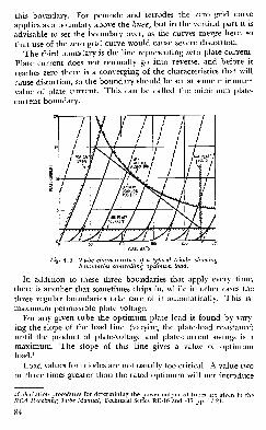
this boundary. For pentode and tetrodes the zero grid curve

applies as a boundary above the knee, but in the vertical part it is

advisable to set the boundary over, as the curves merge here, so

that use of the zero grid curve would cause severe distortion.

The third boundary is the line representing zero plate current.

Plate current does not normally go into reverse, and before it

reaches zero there is a converging of the characteristics that will

cause distortion, so the boundary should be set at some minimum

value of plate current. This can be called the minimum plate-

current boundary.

Fig. 416. Tube characteristics of a typical triode, showingboundaries controlling optimum load.

In addition to these three boundaries that apply every time,

there is another that sometimes chips in, while in other cases the

three regular boundaries take care of it automatically. This is:

maximum permissible plate voltage.

For any given tube the optimum plate load is found by vary-

ing the slope of the load line (varying the plate-load resistance)

until the product of plate-voltage and plate-current swings is a

maximum. The slope of this line gives a value of optimumload .

1

Load values for triodes are not usually too critical. A value two

or three times greater than the rated optimum will not introduce

iCalculation procedures for determining the power output of tubes are given in theRCA Receiving Tube Manual, Technical Series RC-16 and -17 pp. 17-21.

84

distortion, but the power will be reduced somewhat. In triode

output tubes the optimum load is several times the plate resist-

ance—usually three, and often five or more times. Further increase

of plate load improves waveform slightly and increases output

voltage swing slightly, but reduces output power, because the

current swing is cut down more than the voltage swing is in-

creased. Use of a plate load less than about three times the plate

resistance results in distortion, unless the grid input swing is

restricted, which limits the output.

For pentode and tetrode tubes, the term optimum load can

!

i

Fig. 417. Tube characteristics of a typical tetrode or pen-tode, showing boundaries controlling optimum load.

have a stricter meaning. Working at a level a little below maxi-

mum output, variation of the load changes the nature of the dis-

tortion. In triodes, all the curvature is in the region of the mini-

mum plate current boundary, which results in second harmonicdistortion. In tetrodes and pentodes, curvature is also introduced

at the positive grid-swing boundary when the top end of the load

line swings below the knee of the curves, representing load values

higher than optimum. The higher-order harmonics are intro-

duced, and the amount of second harmonic depends on how the

two sources of curvature balance one another. It is possible, byselection of load value, to eliminate second harmonics altogether.

An analysis of distortion from typical tetrode or pentode tubes is

shown in Fig. 418. For some purposes the point where the sec-

85

ond harmonic disappears, or the total harmonic is a minimum, is

considered the optimum load.

We have assumed that the object is to get the maximum output

with minimum distortion. But since in audio work the maxi-

mum output is somewhat of an unused figure, reached at only

fairly rare peaks, it can be said that distortion is more important

at lower output levels. The exact curvature of the characteristic

along any given load line follows a rather complicated law. Theresult can lead to the following kind of experience: Assume the

plate load is made adjustable, so that it can be varied. With a

harmonic analyzer connected to give minimum distortion at or

near full output, turn the level down 10 or 20 db. Readjustment

of the plate load will probably reduce distortion at this reduced

level. Consequently it is probably better to choose a load value

that gives minimum distortion at low levels, even though the dis-

tortion at maximum level may be up slightly.

86

extending design factors

Every book on feedback opens with a light barrage of mathe-

matics, in which the gain of an amplifier with feedback is

shown to be:

A' = A1 + A/?

where A is the gain without feedback and fi is the attenuation of

the feedback path. Then there is a discussion of this, and out of

the hat comes A = 1//3. (Gain without feedback is described

in Chapter 1.) Blinded with science, the reader rubs his hands

and reaches for a soldering iron. However, the gain without feed-

back is not always large. If we are concerned with low-gain

amplifiers or with effects at the edge of the band, we must go

back to the basic equation. We can write this in the form:

1

AjS

+ A/?(55)

When we work in decibels, we have:

db gain = 20 log 1 + 20 log (56)

You will notice an interesting term enclosed in the parentheses.

This is what we have been looking for, because the first term on

the righthand side is just the traditional approximation; the sec-

ond term is the gain component of what has been called the “mu-

beta effect.” This unexpected name was provided by Dr. H. W.

87

Bode. 1 In classical engineering papers you will find the funda-

mental equation written as:

G = 1*

(57)

Notice here that as well as using G in place of A' and p in

place of A, the sign used in the denominator (by Dr. Bode) repre-

sents the magnitude value of /?. Our form is based on the alge-

braic value of p, which is itself negative in the case of negative-

feedback and positive in the case of positive feedback gain. (This

was discussed fully in Chapter 4.) Algebraically, both forms are

essentially the same in the following manner:

G — A' — £— — A1.-W8

-1 - (-/JA) “

1 + Aj8

Before going on to discuss the refinements in calculation whichare provided by the exact formula, let us look at the reasons for

using it. Some of them will probably never affect some readers,

but in special circuit designs this technique is invaluable. Forone thing, it takes the use of positive feedback out of the cut-

and-come-again class, and there’s a big future in positive feed-

back if only to help out in a component shortage.

The first use of the exact equation is to check what happens at

the edges of the band when the gain of the amplifier varies. If youlook up the government specifications for the tubes you are

using, you will see that when the maker says boldly gm = 5,000

micromhos, he really means something between 4,000 and 6,000

or, if you are not a military customer, even wider limits. Roughlyspeaking, that means that the gain per stage can vary over a range

of about 4 db: in three stages, 12 db will be the range for a typical

audio amplifier.

Actual stability, under these conditions, may be a headache in

its own right, but the maintenance of a specified frequency

response often may cause a lot of trouble. A batch of tubes on the

high side may result in the measured frequency response falling

outside the customer’s limits. Try telling him his tubes are too

good!

The second major use for the exact equation is in one of these

multiple feedback loop amplifiers we discussed in Chapter 4. If

we want to design this right to the bitter end, we must determine

Network Analysis and Feedback Amplifier Design”; H. W. Bode, D. Van Nostrand

Co., Inc., New York, N. Y„ 1945; p. 33.

88

the gain and phase characteristics of the first subamplifier with its

positive feedback to draw the phase and amplitude responses for

the complete amplifier, to which the main negative feedback is

applied.

The "alpha-beta" evaluator

These more refined calculations became really practicable in

October, 1949, when Jean Felker of the Bell Laboratories pub-

lished a paper on the subject.2 To avoid confusion, since the

original calculator (called the “mu-beta effect” calculator) wasdesigned from Dr. Bode’s equation, we have modified it to con-

form to our application of the form A/(l -f- A/?) as representative

of negative feedback gain. The original design3 presents \aj3 wherewe have used A/2, and all angular measurement scales are the

supplements of those in the A/2 evaluator. (Where we use 70°,

Mr. Felker uses 110°, etc.) The evaluator is a sort of circular slide

rule for performing the necessary phase and amplitude calcula-

tions.

Let us go back to our mathematics again and see what confronts

us. The alpha-beta (mu-beta) effect is:

A/?(58)

1 + A/2

In general, both A and /3 include a phase shift. Let us take the

total phase shift in the amplifier and feedback network at a par-

ticular frequency to be 9. This is the phase which we use whenwe draw the Nyquist diagram. Since we now have to watch our

signs, we must notice that in the middle of the working range 9

= 0°, while at the danger point for stability, 9 = 180°. We can

write the alpha-beta effect as:

|

a/2| /9— (59)y/0 =

i + |

A/?|

/e_

where y (gamma) is the magnitude of the alpha-beta effect and <j>

(phi) is the phase. We know the phase shift in the feedback net-

work, because we can calculate it using the templates: call this

i[/ (psi). The effective phase shift through the amplifier with feed-

back connected is then <j> -if/. When $ is zero, this is just

2 “Calculator and Chart for Feedback Problems,” Jean Felker; Proceedings of theIRE, Vol. 37, p. 1204.

3 The original “mu-beta effect” calculator is available from Graphimatics, 201 >i.

Taylor Are., Kirkwood 22, Mo.

89

(/> instead of the value without feedback, as given by 0.

The gain of the amplifier is y db plus the ideal gain, 20 log

1//3 db. The Greek letters y, 0, <j> and ip have been used because

they are the same as those in the Felker paper.

For some purposes it is rather useful to turn the mu-beta effect

upside down. Let us write v (upsilon) = 1/y. Then

+ |A/?| /0 1

I

A/?| /_1

- + |A/j| /e

We did not do this bit of mathematics just to show how clever

we are: this particular form is rather a useful one. Consider the

impedance shown in Fig. 501-a. Z is any impedance, and R is a

resistance. Taken together the impedance is R + Z, and this

can be written R (1 + Z/R).

Remembering that Z is a general impedance, we can write this

as

R(1 +[4|./^) (61)

If we put 0 = -O' and A/? = R/Z the impedance of the two-

terminal network is thus Rv/—<f>.

In much the same way, the admittance of the circuit in Fig.

501-b is

¥ + ¥)Now we put A/3 = Z/R and also put 0

mittance equal

2R

(62)

O', to make the ad-

v/—<j>

We can go even further and apply this expression to the net-

works of Fig. 502. If we take the ratio Et/E2 , which is the most

useful when we want to convert to decibels, we have for this ratio:

4r= 1 + l4~ | /^.(Fig. 502-a)

-jr- = 1 + l^H /*' (Fig- 502-b)

-|T = i + (l + |

J^| A /ff, (Fig. 502-c)

Even the impedance forms are useful in decibels, because when

90

we connect an impedance as the plate load of a pentode, the gain

is gmZ, or (20 log gm + 20 log Z) decibels. For that reason the

curve of u given as Fig. 503 shows v in decibels.

We could, of course, proceed to use those curves to determine

the alpha-beta effect, but the Felker calculator is much moreconvenient. This chart (in modified form) is reproduced in Fig.

504. When the rotatable arm is fastened to a suitable backing of

thin card or plastic and attached to the center of the circular chart,

the longer end of the moving arm moves over the upper semicircle.

The readings obtained on this scale represent the alpha-beta effect

as measured in degrees.

Fig. 501. Some typical circuits employed in solvingtwo-terminal network problems. In (a) the imped-ance (Z) is in series with the resistance. In (b) , the

impedance is in parallel with the resistance.

Figs. 505 and 506 have been constructed to enable us to work

out an example. Three circuits of 6 db per octave are assumed,

with characteristic frequencies at 1, 2 and 4y/2. The most feed-

back which could be applied without instability is 21 db and for

this example we shall assume that we are applying 15 db of feed-

back. We can now therefore construct the second scale, markedA/S, with its zero at the 15 db down level on the gain belowmaximum scale.

Using the evaluator

Now take the evaluator. At <o = 2, we have alpha-beta = +4db and 6 — 130°. Find the point where alpha-beta = +4 and

alpha-beta phase = 130°. It is up near the top left-hand side of

the chart. Turn the rotating arm until it passes through this

point, and read off the alpha-beta effect magnitude on the armitself and the phase on the semicircular scale. We find +2.3 db,

140°. Repeating the calculation at other points, we get +6.2 db,

88° at to = 2\/2, and so on. All these values have been plotted

in on Figs. 505 and 506. In Fig. 505, you will remember, this

alpha-beta effect is the deviation of gain from what we expect

in the simple theory. We use the alpha-beta scale for plotting the

response. As you can see, the “flat” gain is about 1.5 db below

the zero determined by the simplified theory. The phase shift is,

at most frequencies, much less with feedback, but at the edge of

91

the working band it rushes sharply upward. You can see howdangerous this can be in a multiple-loop amplifier, by considering

the values at « = 4: with feedback the gain is 1.5 db above the

“flat” region, but the phase shift has practically hit the 180° mark.

a b c

—° Fig. 502. Some typical impedance

E2*problems in four-terminal networkanalysis are represented by the circuits

0of (a), (b) and (c).

As a subamplifier in a complicated multiloop system this partic-

ular system could give you enough headaches for a lifetime.

Suppose that, in place of the gain we planned, the amplifier

has in it rather old or low-limit tubes. The gain without feed-

back A may have dropped 6 db. The feedback term j3 remains the

same, however, so the product A/3 (alpha-beta) is down 6 db. Thealpha-beta scale zero, on the left of Fig. 505, should now be set

at 9 db on the gain below maximum scale. At w = 2 we have A/3

= —2 db, 6 = 130°, so that the Ap effect is +0.2 db instead of

+ 1.6 db. As to 0, the response for Ap = 9 db and 6 = 0° is

2.6 db. The response therefore has risen 2.8 db at w = 2 for this

low-gain case, instead of 3.1 db for the normal gain case. Themid-band gain has dropped 1.1 db.

Fig. 503. Graph showing the impedanceforms of Fig. 502 plotted in db. Theformulas used to derive these curves (see

text) are based on the relationship ofEj/Ej. In the case of a pentode tube,

when the plate load is an impedance,the gain is gmZ or (20 log gm + 20 log

Z) decibels. Thus, these forms are quite

useful in practical work.

We are not inclined to discuss this application of the alpha-

beta evaluator any further, since the time that would be spent

on additional discussion can be spent more profitably in working

out the solution to some of the many typical problems you are

likely to encounter in audio amplifier design work. However, here

is an important item: When the feedback network itself contains

reactances, which usually will be capacitors, the response calcu-

lated is that which appears at the output of the feedback network.

Therefore it is necessary to subtract the response of the feedback

network from the calculated response given by the alpha-beta

92

evaluator to get the response for the overall system. This is shownin the basic equation:

gain = 20 log1

Jalpha-beta effect.

Fig. 504. The Alpha-Beta evaluator. This chart is a modified version of the Felker“mu-beta effect" calculator discussed in the text. Familiarity with its operation will

aid considerably in amplifier design work.

Here is another use for the alpha-beta evaluator. It can be

used for determining the stability margin directly. As you mayremember, we showed in Chapter 3 that a quantity called the

stability margin was a very useful measure for the safety of a

93

(64

)

design. This quantity is in our notation:

A' 1

A ~1 + A/?

The alpha-beta effect, you will remember, is

A/3 _ 1

7 “i + r~

AjS

If we have a value of, say, 6 db for A/J, and we calculate the

A/? effect corresponding to —6 db, the quantity we obtain is the

stability margin. Let us draw up a table from Figs. 505 and 506

as follows:

CO : 1 1.4 2 2.8 4

A(3 - +10 db +7.5 db +4.2 db -1 db -6.3 db

9 = 83° 1 05 c 130° 154 176°

A/3 effect = -0.8 db +0.3 db +2.3 db +6.2 db -0.5 db

Stability

Margins = -10.8 db -7.3 db -1.8 db +7.2 db +5.8 db

The last line was calculated directly, taking the -10 db, 83°,

-7.5 db, 105°, etc. points on the chart. This means that it is not

necessary to pass through the response, alpha-beta effect or overall

response system in order to check the stability margin. When the

feedback path has a nonuniform response this can be very helpful,

because all that need be done is to plot the two pairs of curves,

for alpha-beta and for beta, and then determine the stability

directly.

There is a very attractive phrase which you can find in British

patents: “Having now particularly described and ascertained the

nature of the invention . ..” Well, we’ve done that, but just in

case the explanation has not been sufficiently certain, Fig. 507

shows how the evaluator is actually set to fish out the results at

co = 2. The point marked A is at alpha-beta = +4.2 db, alpha-

beta phase = 130°. The rotating arm OA has been turned until

the edge passes through this point, and the alpha-beta effect is

read off at A on the scale printed on the arm. The phase of the

alpha-beta effect is read off on the circular scale. For the stability

margin we hunt out point B, -4.2 db, 130°, and twist the arm to

pass through this point. The stability margin is read off the arm.

94

Wary readers may have noticed that almost everything we have

discussed in this book deals with the analysis of feedback circuits

and not the synthesis. We guess a circuit and test it, on paper,

to see if it will work. Nearly everything in the field of circuit

design boils down to this in the end. The main differences appear

in the methods of testing. At one extreme you wire up the circuit

Fig. 505. Graph showing three designcurves of an amplifier. Curve A is theideal response, curve B is the responsecalculated with the Ap effect, and curveC is the response calculated without

feedback.

and pray; at the other extreme you test on paper in such a general

way that you never come to a practical answer. This work aims

at a reasonable compromise. While providing all the information

Fig. 506. This graph shows two curvesrepresenting amplifier phase shift char-acteristics. Curve A is the shift withoutfeedback; curve B is the shift with feed-

back.

needed by the average professional designer, we hope also it is

not too forbiddingly mathematical for the man who wants to

95

build just one amplifier, but wants to build it right. The impor-

tant thing to learn here is: alpha-beta simplifies design work.

Design comparisons

Having been associated with a group of network engineers, it

was unavoidable that we run across a concept of theirs which

stated simply: All problems are network problems, and all net-

work problems are low-pass problems. You may wonder what this

has to do with the problems of designing feedback amplifiers, but

you will find it a valuable approach to keep in mind.

MOVING ARM IN POSITION FOR A0 EFFECT

This preamble is intended to introduce a design procedure for

narrow-pass bandpass amplifiers (which are more commonly

known as i.f. amplifiers) and to show that they may be designed

in complete accordance with the rules we have already discussed,

just as though they were audio amplifiers. This is not to say that

you can build a radar i.f. amplifier for 60 me in the same way

you build an audio amplifier. But you can design a three-stage

amplifier with 20-db feedback for use at, say, 1 me without any

design curves other than those which we have already used.

Although it will appear that this type of amplifier is limited to

special applications, it is in itself noteworthy as a source of design

comparisons, particularly when approached through the network

concept.

Procedures

The basic unit we shall consider is that which is sometimes

96

known as the center-tuned, resistance-loaded amplifier. The plate

circuit of each tube contains a parallel network of resistance, in-

ductance and capacitance. Each circuit is tuned to the center

frequency. This type of amplifier is easier to design as a feed-

back amplifier than the stagger-tuned type, in which the plate

circuits are tuned to different frequencies. The center-tuned

Fig. 508. The basic parallel reactance circuit is equivalent to

a capacitance under certain conditions. Since in theoretical cir-

cuit design development, mathematical calculations are moreeasily obtained using admittance than with reactance, in this

circuit the admittance (Y) is equal to j0>C -f-l/j^L.

type is also easier to line up, because three or more reference fre-

quencies are needed in the stagger-tuned variety. In the latter

case the spacing of these frequencies governs the pass character-

istic and a good signal generator must be used.

Let us look at the basic element of the circuit. This is shown

in Fig. 508 and consists of inductance L in parallel with capaci-

tance C. The admittance of this circuit is jwC -f- 1 /jwL.

Notice that it is easier to use admittance (than reactance) whenyou deal with parallel circuits. In theoretical work admittances

make mathematical manipulations easier.

Fig. 509. L and C replace the inductance in the series bandpass circuit

with lowpass equivalence. In this arrangement, the circuit impedance(Z) is equal to jaiL -)- 1/jaC. Characteristics of the circuit and related

mathematical derivations are covered in the text.

We will do some manipulations and see what we can make of

this admittance:

Y = jwC + ji <65

>

Adding the two over the common denominator j«L, we have:

Y (jwC)(j(oL) + 1

“ jtoL

Multiplying the numerator we get:

Y = j2(P2LC +1juL

Sincej= then

j2 = -1. We then get:

-co2LC + 1

~ jtoL

97

(66)

Rearranging this equation gives us:

Y 1—

w

2LC~ jwL

Now let w 2LC = 1. This will be the case at the antiresonant

frequency w0 :

^ = vn <67>

At this frequency the admittance Y is zero and the circuit of

Fig. 508 is at resonance:

At this frequency 1/ w0L = co0C (the reactance of the coil is

equal to that of the capacitor) . We can write the coil reactance as

coL — w0Lw0

and

w 2LC r -^<002LC =

w0‘

w2^

w02

because w02LC = 1 and l/jw0L = jw0C.

The expression for admittance can be changed to:

Y = )(68

)

Suppose to save space and trouble, we let Q (capital omega)represent

ww0

in our further calculations. The admittance is then simply:

Y : jfiC (69)

For a single capacitor, the admittance at a frequency w is just

Y = jwC.

The reader will be well advised to think about these two equa-

tions very carefully. He will see that anything which can be said

about a capacitance at a frequency w can be said about an anti-

resonant (parallel) circuit at a “normalized frequency” O. Forexample, 1,000 jqif has an admittance of 1/16,000 ohms at 10 kc.

98

Put 100 [xh in parallel, and the antiresonant frequency is 500 kc.

This means that <o0 = 2tt X 500,000 and at this frequency to = <o0

(70)

The admittance is zero, just as the admittance of a capacitor

alone is zero at zero frequency. Raising the frequency slightly to

505 kc:

y 505 \ 2

500,000 -W _ i

500

O = 2tt x 500,000 t t1 -0

;;

- 11

0 = 2tt x 500,000 X -02

n = 2tt x 10,000

and the admittance joC is .0000628 mhos, corresponding to an

impedance of 16,000 ohms. The admittance at 5 kc from the

center frequency is equal to that of the capacitor alone at twice

5 kc from zero. We shall get the same number if we examine the

admittance at 495 kc, but the sign will be negative because it

represents a negative or inductive susceptance instead of a posi-

tive or capacitive one.

The admittance of an antiresonant circuit f cycles away fromthe tuning point is equal to that of the capacitor alone at 2 X /

cycles away from zero. To help the reader who wants to check

this, the approximation used is (1 + A) 2 = 1 + 2A, where A

(lambda) is a small fraction of 1.

We can do the same thing for the series circuit of Fig. 509.

Here the impedance is:

jnL _ j«L -)-

jtoC

(1 - tj2LC)

jwC

(Do

with n having the same meaning as before.

Let us look at a very simple application of this result. A low-

pass filter has been designed in the form shown in Fig. 510. It

may have been designed by a purely arithmetical process to give a

special response. Now we want a bandpass filter to give the cor-

99

responding performance symmetrically centered on a “carrier”

frequency.

First of all, remember that there is a factor “2” in the low-pass

to bandpass transformation. If we want the bandpass filter to

work up to f cycles on each side of the center frequency, we must

make the low-pass filter have a design cutoff of 2f cycles. Wehave seen that we can replace a capacitance by an antiresonant cir-

Fig. 510. Substituting Figs. 508 and 509, low-pass filter circuit (a) becomes bandpass cir-

cuit (b). Added elements tune the circuit to

center frequency.

cuit with the same capacitance (allowing for the factor “2”) and

that we can replace an inductance by a resonant circuit with the

same inductance. The bandpass filter is thus obtained by using

the circuit shown in Fig. 510. The added elements are those

which tune the low-pass components to the center frequency.

The bandpass problem is just a variant on the low-pass problem.

Now we may look back to the circuit we need for our ampli-

fiers. This is shown in Fig. 511. We can write the admittance

of this as 1/R jnC and remembering the equations we used in

setting up our templates (Chapter 1), we can say that the circuit

has a characteristic frequency O given by OCR = 1 . At this fre-

quency, which is most conveniently written n0 = 1/CR, the

response is 3 db down. It is at a distance <oa from the center fre-

quency, and <Da = 1/2CR.The low frequency and bandpass circuit responses are shown

together in Fig. 512. This is drawn in the usual “response” form

Fig. 511. Plate loads of a typical bandpass ampli-

fler- At the left the load consists of merely a resist-

:c §jl ance and capacitance in parallel. At the right, an3 inductance (L) has been added to this combina-

tion as another shunt element.

without decibel and logarithmic scales, so that the relationship

between the two curves and the usual universal “resonance curve”

of the textbooks is made more obvious.

The way in which the factor “2” appears can also be remem-bered by considering these two curves. It will be seen that for

any C-R the total bandwidth is the same. In the low-pass case

this means that the band extends from 0 to f; in the bandpass

100

case it extends from f0 — i/2 to f0 + i/2. There are a number of

ways of interpreting this mathematically, but they are all beyond

our scope. Perhaps the only thing we need to mention is that the

noise energy is the same wherever you put the band.

Notice also that the low-pass case is not simply a bandpass

extending from -f to f, centered on zero. This produces an error

of 2. The bandwidth 3 db down is the same for low-pass and

bandpass, but because there are two sidebands, the audio width

is halved in the bandpass case.

One more point to observe: For our purposes, the bandwidth

is taken at the 3 db down level. You will find very often in text-

books that the 6-db point is used, but this has no significance for

our design technique.

Fig. 512. Lowpass and bandpass circuit

responses. These curves are shown to-

gether so that their relationship as

compared to the universal resonancecurve of textbooks becomes more ob-vious. The lowpass response is shownat the left; the bandpass response at

the right. The range of the curvesextend from /0 — /2 to f0 -j- f2 (see

text).

Let us now turn to our specific task, the design of a bandpass

amplifier with feedback. We shall take the center frequency to

be 1.6 me, so that to0 = 2tt X 1.6 X 10® = 107, and the bandwidth

to be 16 kc (8 kc on either side of the center frequency). Fromwhat we have just said, this is really equivalent to designing an

audio amplifier to work up to 16 kc. We shall use two 6AK5’s

and a 6AQ5, since this is a paper design. Let us see what we can

do with a three-stage amplifier.

For the 6AK5 we can rely on having a transconductance of 4,000

pmhos, and we shall be safe in taking an input capacitance of 7

ppf and an output capacitance of 5 ppf. The capacitances of the

6AQ5 are higher, and we must assume about 10 and 15 ppf. Thebook values are lower than this, but the socket must be taken into

account. The optimum load for the 6AQ5 is 5,000 ohms, so that

with decoupling the stage gain in the output stage is 20 times.

Since in this sort of amplifier we usually apply the feedback fromcathode to cathode, the first and third stage cathodes will not bedecoupled, and the output stage gain is only 10 times.

It is important to notice that the plate circuit of the 6AQ5should not affect the behavior (from the stability point of view)

of the amplifier since the feedback comes from the cathode.

.RESPONSE

0%-aig a>„ a'o+O'irFREQ

101

Theoretically we have only two circuits in the feedback loop, andtherefore it must be stable, whatever we do. But let us look at

the first plate circuit. The total capacitance is made up of the

output capacitance of the first tube and the input capacitance of

the second tube: this gives us 12 pgf. With wiring, coil capaci-

tance and an allowance for trimming let us increase this to 25

ppf. The bandwidth is 16 kc, so that we can be 3 db down at the

band edges if we have,

27T x 16,000 x 25 x 10-12 X R = 1

and

R = 400,000.

This implies that the Q of the coil must be 100, which is a

moderately good coil. Let us take this as one circuit. The stage

gain, without decoupling, will be about 800 times. Using the

templates of Chapter 1, wTe draw the sideband responses, putting

at 50,000 (2tt X 8,000). Adding another circuit with <oa at

200,000, we get overall curves which show that the phase marginfor 20-db feedback is 45°, which is a fairly safe value.

At first sight this looks like a reasonable design. The second

circuit, for which wa = 200,000, has a capacitance of the same order

as the first, if we make slightly less generous allowance. It is easy

to see that for this circuit R = 100,000, and without decoupling

the stage gain will be 200 times. This means that the total gain

is 800 X 200 X 10 = 1,600,000, or over 120 db.

In theory, all we do now is calculate the inductances and con-

nect a feedback resistor, cathode-to-cathode. In practice we have

left out a very important factor, the plate-grid capacitance of the

tube. Consider the second tube. The impedance in the grid cir-

cuit is 400,000 ohms; the plate-grid capacitance is at least .02 upt

even without strays. This capacitance has an impedance—at 1.6

me—of 5 megohms. As a rough approximation of the plate swing

0.4 meg .4 1

5 meg + 0.4 meg—

5.4—

13.5

will be fed back to the grid.

We have ignored the phases, because we want only a rough

figure for the moment. Thus, with almost one-tenth of the plate

swing reappearing at the grid, we cannot use a gain of 200 times.

Our design procedure breaks down because it leads us to values

which are not practical in this case.

We get around this problem by checking on the grid- plate

102

capacitance first. We know it is 5 megohms, so we can construct

a table:

Plate load

Plate-grid

feedbackratio

Gain for

g nl—4,000and no

decoupling

100,000 50 200

50,000 100 100

25,000 200 50

20,000 250 40

10,000 500 20

This table is used in conjunction with the required gain, which

we haven’t mentioned so far. Let us take a figure of 50 db, with

20-db feedback. Without feedback we need 70 db, and the out-

put stage will give us 20 db. By using plate loads of 10,000 ohmsin each of the first two stages, giving 26-db gain in each (20 times),

we get a gain without feedback of 72 db, which is near enough.

Having fixed R, we can go back and calculate the capacitances.

We have, for one stage,

2tr X 16,000 X 10,000 C = 1

c = xmow = 1 -000

For the other stage, with four times the bandwidth, we find that

C = 4,000 ppf.

103

The output stage, which has a resistive load of 5,000 ohms, will

give a response 3 db down at the band edges if we should nowmake the total capacitance 2,000 ppf.

We now calculate the inductances which must tune these capac-

itances to 1.6 me. They are:

1. 1,000 ppf 10.0 ph2. 2,000 ppf 5.0 ph3. 4,000 ppf 2.5 ph

Calculation of these values were obtained by using the formula:

f :

1 _ (72)0

2tt VLCRearranging the formula to solve for L:

VL =2*f VC1

(27rf)2C

Substituting values in this equation we have, when C = 2,000

ppf:

T 1 _ 1 K u“40(1.6 X 106

)

2 X 2 X 10-® “ 204.8 X 10s- ^

With this information, the amplifier design is almost complete.

The 6AK5 does not like more than 180 volts on the plate, at 7.7

ma. We can put the 10,000-ohm resistors in the plate-supply

leads to drop the voltage and use the 250-volt line for the 6AQ5.The coils are then connected in the grid circuit, as shown in Fig.

513. The gain from the first grid to the third cathode will be

about 200 times, which we propose to reduce by a factor of 10.

The feedback resistor therefore must be approximately 20 times

the cathode resistance, Rk .

What more remains to be done? This depends on the design

specification.

We can compute the stability margin in the manner described

in Chapter 3. We can calculate the exact response, using the

alpha-beta evaluator described earlier in this chapter. We can,

if needed, put a network in the feedback path to make the response

drop more rapidly outside the working band. This network,

which corresponds to a capacitance in the ordinary audio ampli-

fier, has been shown dotted in Fig. 513.

104

The example we have chosen is a very simple one, because the

use of feedback in high-frequency amplifiers seems to afflict a

lot of people with quite unnecessary feelings of nervousness. As

you can see, it is just the same sort of problem you encounter at

audio frequencies, except that the screen decoupling, plate de-

coupling and band-center (or low end at audio) effects can be

neglected. In fact, audio amplifiers are really more difficult to

design!

Why feedback so far?

At first glance, the general idea behind feedback seems sound

enough: Plenty of feedback improves amplifier performance, and

Fig. 514. The two standard feedbacksystems as considered from the outputend. At (a) is an example of voltage

feedback; at (b) is an example of cur-

rent feedback.

to get a large amount of feedback we must feed back a voltage

from the output to a stage where the signal voltage is quite small.

Blind acceptance of this fact as the only requirement has encour-

aged the design of a number of amplifiers in which feedback is

applied from the output stage back almost, if not quite, to the

input stage.

The owner of such an amplifier will probably be all too familiar

with some of the problems attending overall feedback, but there

are others that are perhaps less obvious.

Many proud possessors of high-fidelity equipment have been

puzzled by experiences like this: The complete chain sounds

horrible—shrill resonances, intermodulation and other forms of

distortion. A check of the amplifier with dummy load shows

everything all right in that part of the system; the speaker sounds

fine on another amplifier; all impedances match correctly. Thechain works nicely on phono input but not on radio (or maybe

vice versa), but everything is all right when a different speaker is

used. Where does the trouble lie? To see how such snags arise

let’s consider first how feedback is obtained.

From the viewpoint of the output end there are two kinds of

feedback: voltage and current. See Fig. 514. In the first (Fig.

514-a) the signal fed back is proportional to the voltage developed

across the output load; in the second (Fig. 514-b) it is propor-

105

AMPLOUT;

TC

V01WGE FEEDBACK CURRENT FEEDBACK

tional to the amount of current drawn by the output ioad.

From the viewpoint of the input end there are two methods

of applying the feedback: series injection and shunt injection.

See Fig. 515. In the former the signal feed back is injected in

series with the original input signal (Fig. 515-a), while in the

latter (Fig. 515-b) it is injected in shunt with it.

Fig. 515. Examples of two methodsemployed for feedback injection as

they are viewed from the input end.

Series injection is shown in (a); shuntinjection is shown in (b).

A point that is often overlooked is that when the feedback loop

includes both the input and output circuits of an amplifier, the

impedance of the input-signal source and of the output load affect

the amount of feedback.

For example, with voltage feedback, if the load impedance is

reduced to zero there will be no feedback at all. Similarly, when

current feedback is used, there will be no feedback at all if the

load impedance is an open circuit.

At the input end of the amplifier the method used to inject the

feedback depends on the impedance of the signal source. With

series injection the source impedance connected to the input must

be low compared to the grid-circuit impedance of the first stage

or it will reduce the amount of feedback. If the input source

impedance becomes an open circuit there is no feedback.

In practice the input circuit is closed either by the secondary

of an input transformer or by a grid resistor so that there is

always a complete feedback path, although the impedance con-

nected to the input will still modify the feedback characteristic

somewhat.

Shunt feedback injection depends on the source impedance

connected to the input being high, since a short circuit across the

input will reduce the feedback to zero.

The reader is probably quite familiar now, with the properties

of inverse feedback in improving frequency response, reducing

distortion and modifying input and output impedances. Forexample, the internal output impedance of the amplifier, whichserves as loudspeaker damping, can be reduced considerably bythe liberal use of inverse feedback. Similarly, the input imped-ance can be modified—made either higher or lower—according to

106

whether series or shunt injection, respectively, is used.

Where an input transformer introduces an undesirable reson-

ance peak, appropriate connection of the feedback circuit maydamp out this resonance and produce a satisfactory overall re-

sponse. But a change in the load impedance connected across the

output will alter the actual amount of feedback reaching the in-

put, and thus change the effective response of the input trans-

former again. Similarly, changing the input impedance can some-times affect the damping at the output.

Fig. 516 . Circuit of a typical amplifier employing overall voltage feedback.

With overall feedback this interaction is always present, even

though it may pass unnoticed. An effect that does not pass

unnoticed, however, is that the stability of the amplifier depends

on the impedances connected to it. For example, an amplifier

with overall feedback like the one in Fig. 516 may be perfectly

stable with a 3-ohm loadspeaker of one particular make; but someform of instability may show up when another speaker of slightly

different impedance is connected. In addition, many amplifiers

with overall feedback are not stable when the output load is dis-

connected or if a 15-ohm loudspeaker is used in place of a 3-ohmtype.

Various arguments in their favor have been used by designers

and manufacturers of such amplifiers, but with a really goodamplifier we should not need to be so fussy about the impedancesconnected to it. Correct matching is obviously desirable, but onecannot prevent the loudspeaker impedance from having a fre-

quency characteristic (Fig. 517) and affecting the feedback.

Internal noiseAnother feature detracting from the advantages of overall

107

feedback is its effect on output hiss and other noises generated in

all high-gain amplifiers. It has generally been preached that

inverse feedback, however used, reduces distortion and noise, but

this is not quite true. Harmonic and intermodulation distortion

are periodic signals added to the original signal. With inverse

feedback we can build up an out-of-phase component of the dis-

tortion signal and combine the two so as to reduce it. But noise,

especially output hiss, is not a periodic signal. Rather, it is a ran-

dom movement of charges or currents occurring over an infinitely

wide range of time intervals so that it contains frequency com-

ponents effectively from zero to infinity. It is true that the fre-

quency response of the amplifier restricts the range of noise fre-

quencies that reach the output, but the foregoing statement is

true at the point where noise is generated. This means that to

neutralize noise completely an out-of-phase signal of the sameamplitude must be fed back absolutely instantaneously coincident

with each “happening.” The fact that every amplifier has a re-

stricted frequency response makes this impossible, so it is obvi-

ously impossible for feedback to produce the same cancellation

for noise that it does with distortion.

Taking the overall result when inverse feedback is used, extra

gain is required to offset that used up by the feedback. Thismeans that in a feedback amplifier, noise will receive far moreamplification in the output than in the same amplifier withoutfeedback. If feedback could cancel noise to the same extent that it

can cancel harmonic distortion, the noise would finish up at

about the same level as in the amplifier without feedback, pro-

vided the overall gain remained the same. But because the

inverse feedback is unable to cancel the noise as completely as it

does the periodic distortion waveforms, the resulting noise in the

output of the feedback amplifier is actually higher. This explains

108

what some workers have noted: that a feedback amplifier seems

to have more hiss than a nonfeedback amplifier with the same

gain but without feedback.

The alternative

All these disadvantages of overall feedback can be overcome by

restricting the number of amplifier stages over which feedback is

applied.

a 6

Fig. 518. Two types of short loop feedback. In (a) the voltage is often insuffi-

cient for employing large amounts of feedback. In (b), the resistor (R) absorbstoo much of the available power.

Fortunately, coupling impedances between stages are not sub-

ject to variation as source and load impedances are, so the possi-

bility of impedance changes at both ends of the loop no longer

arises. It is generally unnecessary to apply feedback to reduce

distortion in the early stages of an amplifier where signal level is

so small that curvature distortion cannot arise anyway; in fact, it

is better to operate the low-level stages at maximum gain to main-

tain a good signal-to-noise ratio. Sometimes single-stage feedback

may be used in a low-level stage for tone control, but this can

still be applied after sufficient amplification has been provided to

overcome output-hiss troubles.

Applying inverse feedback from the output over not more than

two stages—and preferably only as far back as the driver stage-

will prevent instability troubles with changes in the output load.

It can even improve amplifiers that are perfectly stable with over-

all feedback, but whose performance may be affected in other waysby changes in the output load.

The next question is: Why hasn’t this short-loop feedback ar-

rangement been used more before this?

The difficulty

When it comes to applying feedback from the output of anamplifier to the driver stage, the difficulty that arises is that the

109

signal at the point to which feedback is applied is not very muchsmaller than at the point from which it is obtained. If the feed-

back is taken from the low-impedance secondary of an output

transformer (Fig. 518-a), the voltage may not be high enough to

give as much feedback as you want. On the other hand, if feed-

back is taken from the primary of the output transformers (Fig.

a i

Fig. 519. Two better types of feedback circuit. The results obtained with the

use of these circuits is considerably better than with the circuits of Fig. 518.

In (b), L is a tertiary winding.

5 1 8-b), there is plenty of voltage available, but the voltage-divider

resistors required to produce sufficient feedback at the cathode

of the preceeding stage are so low that they absorb an appreci-

able proportion of the available output power, which is clearly

undesirable.

The solution

Basically, the solution is fairly simple, but (as usual) there is

a practical snag which explains why it has not yet been morewidely applied. As we have explained, the impedance on the

primary side of the output transformer is high, so that, although

more than adequate voltage for feedback purposes is available,

the feedback resistor chain will absorb more current than can be

spared. On the transformer secondary the resistance of the feed-

back arrangement absorbs negligible energy because plenty of

current is available, but the voltage is insufficient. What we needis an impedance between these extremes.

The output transformer can still provide for direct connection

to the voice coil, if it has taps on the primary (Fig. 519-a) or anadditional winding (Fig. 519-b) so that a suitable intermediate

impedance point is available for feedback purposes. The sep-

arate-feedback-winding (tertiary) method is preferable becauseit eliminates the blocking capacitors needed when taps on the pri-

mary are used. Because the feedback circuit consumes negligible

power, the tertiary can be wound with fine-gauge wire and needoccupy only negligible space.

110

drivers and inverters

chapter

6

The majority of amplifiers in the 5-watt class and higher nowuse push-pull output stages. The properly balanced push-pull

stage produces no even harmonics, though that is not so impor-

tant, now that we use so much negative feedback. The output

transformer has no d.c. polarization, which makes it a lot easier

to design (though we must allow for at least 10% unbalance in

any practical circuit) and the signal does not appear in the plate

supply lead, which makes decoupling much less of a headache.

There are other aspects, too, such as the possibility of pushing

down toward class B working. If the tube cuts off in a single-

sided stage, no amount of negative feedback will help the situa-

tion, because just at the instant of cutoff there is no gain, and thus

no A/?. In a push-pull stage one tube is working away to keep the

gain up even when the other grid is far negative, and the feed-

back can do its work in keeping down the distortion.

There is not much point in using push-pull in the early stages

of an amplifier, unless you want to go down to zero frequencyand keep a balanced input. The electroencephalograph designers,

who want to watch your brain ticking before they try to find whatmakes it tick, use these all-push-pull amplifiers so that they canrecord the push-pull signals from electrodes on your head. Thisin itself is a special problem. For most of us, single-sided stages

at low levels, then a phase splitter and a push-pull stage, are theanswer.

While writing this book, we skimmed through a collection of

111

commercial circuit diagrams to see what other designers thought

about phase splitters. Right then we decided that phase-splitting

techniques were not as familiar as we had believed, because the

most commonly used circuit was a pretty poor one, with plenty of

disadvantages and practically no advantages. It does seem worth-

while to make a survey of the known phase splitters and to indi-

cate how good or bad they are.

Fig. 601. The effect on the signal outputwaveform from a class-B pushpull amplifier

stage if one half of the stage is driveni?' twice as hard as the other half.

First of all, why should we concern ourselves with makingthe phase splitter good? We can see the answer most clearly if

we consider a class B output stage. Fig. 601 shows in a very

exaggerated way the appearance of the output from a push-pull

class-B stage if one-half is driven twice as hard as the other. Asyou can see, there is quite a lot of distortion.

More serious, perhaps, is the fact that if the upper half is at

maximum drive, the output power is down to ($4)2

,or little

more than one-half, of the true maximum. The negative feedback

could help the distortion, but it will not get back that extra

power.

Another point comes out of this figure. The hard-working tube

will take an additional plate current of Ii, while the idler takes

only I 2 , so that the output transformer will be subjected to a sub-

stantial polarized magnetic flux which may (if it is not overgen-

* Fig. 602. An ideal phase splitter. Thisconsists of a transformer, capable of pro-ducing equal voltages across the twohalves of the secondary at all times dur-ing which the rated xtoltage is applied

-* across the primary.

erously designed) cause stability trouble at low frequencies,

trouble which can be caused also by the unbalanced signal backin the plate-supply unit.

There may be some more reasons for making sure that the

push and pull are equal, but certainly there are no reasons for

allowing them to be unequal. One of the main problems of

push-pull design is therefore to make sure that the two drive

halves are equal, retaining this ratio at all frequencies, and that

112

they do not change with age. As we shall see, the difficulties arise

when we demand equality at all frequencies, and when we de-

mand that the drives shall stay equal as tubes age and supplies

vary.

Two good phase splitters

The best of all phase splitters is the transformer, shown in Fig.

602. A well-designed balanced transformer will produce equal

voltages across the two halves with an accuracy of 1 part in 1,000

Fig. 603. Another type of phase splitter. J"~

Th is circuit has limited use, but is of con- <siderable interest when the input source

has no ground. The values of the two f(\j

resistors (R) should be equal.

and will certainly stay like that. The main objections to the

transformer are that its frequency response is not too good andthat it makes the use of negative feedback a lot more difficult.

Transformers are mainly used, indeed, when other circuit de-

mands must be met. One example is in operating a push-pull

rectifier, for which the low direct-current resistance of the trans-

former is important; another is in driving a push-pull variable

stage in a limiter or compressor, when the gain control bias musthave a low-impedance path with no time-constant to the grid.

Apart from these special circuits, the interstage transformer is rare

nowadays, although it was standard practice in the early days of

push-pull.

Another excellent phase splitter of limited use is made up of

Fig. 604. A typical application of the cir-

cuit of Fig. 603. The ground on the tunedcircuit does not affect its balance. Thiscircuit was first developed in the year

mr.

two resistors (Fig. 603). This is of interest when the input source

has no ground; for example, if a phonograph pickup or mag-netic reproducing head is to work straight into a push-pull cir-

cuit. Since the same current flows in series in the two resistors

they must be equal in order to give the same voltage at the twopush-pull terminals, and any stray capacitances must also be equal.

An application of this idea has been allied to the diode de-

tector, which gives the circuit shown in Fig. 604. The ground on

the tuned circuit does not affect the balance of the circuit, be-

cause to audio frequencies the tuned circuit is a very low imped-

ance. Now that crystal diodes are so cheap, we consider that a

more economical solution would be obtained by putting a tap

on the center of the coil and rectifying the two halves with sep-

arate diodes. (The circuit of Fig. 604 dates back to 1934).

Fig. 605. One of the more common types of

inverter circuit used today. VI is driven by

the unbalanced input, while V2 receives its

drive from the voltage divider. Althoughpractical, this circuit does not receive too

wide a usage by the critical design engineer.

Some circuits from life

These circuits are, of course, the textbook type, well suited to

the student and ignored by the engineer. Let us turn to a more

practical circuit, which, though very widely used, is not very satis-

factory to a critical designer. It is the circuit given in Fig. 605.

In this circuit VI is driven by the unbalanced input, while V2receives its drive from the voltage divider made up of R and

(n - 1)R. These values provide a drive voltage for V2 of Ei/n.

We can assume that R is very large indeed and that we are using

pentodes. These assumptions have no influence on the final con-

clusions, but they make the mathematics very easy, with A =gmRi instead of

V2 has a gain of gmRi (where gm is the transconductance) , so

114

(74

)

that the voltage applied to its grid is Ei/n. Thus we have

£ ogmRlEi

n

We want this voltage to be equal to Ei, and therefore:

n = SmRl (76)

What could be more pleasant: just look up gm in the tubehandbook, choose R x to suit the tube and you know n right away.

f5

Fig. 606. This diagram shows how the circuit

of Fig. 605 operates.

The total grid resistor nR = R + (n — 1)R will be 100,000 ohmsperhaps, so that R is known too.

The only trouble is that although the tube manual may give

gm = 7,650 pmhos—and we have seen this exactness used—a look

in the MIL specifications will leave you slightly worried. Mosttubes have a tolerance of about 20% on transconductance. If youset the circuit up with a high gm tube, it will be more than 30%out of balance with a low-gm tube. Of course, there are the toler-

ances on the resistors too; although you can always adjust the cir-

cuit to take account of these, you cannot prevent the balancedrifting away as the tube gets old.

Another weakness

If we redraw the circuit as shown in Fig. 606, we see a new dis-

advantage, which we shall find is common in phase splitters. Theoutput voltage to the push-pull stage which appears at A has

passed through one tube (VI of Fig. 605), while that whichappears at B has passed through tubes VI and V2. Thinkingagain of a class-B output we can see that, if we feed back to the

115

grid (or cathode) of VI we shall be feeding back around two

stages for one half-cycle and around three stages for the other

half-cycle. The plate capacitance of V2 provides at high fre-

quencies an additional phase shift which may make the amplifier

unstable. It is not uncommon with circuits of this kind to observe

a short buzz of h.f. oscillations on one peak of a low-frequency

signal. This effect usually is to be detected only with an oscillo-

scope, and its cure involves the addition of as many components as

would be needed for a more sophisticated phase splitter.

Fig. 607. Another little used circuit. The maindisadvantage here is if the tap on the outputtransformer is chosen at a point that will give

good low-level balance with a poor tube, when a

high gm tube is used as a replacement, it will

oscillate, since its normal level lies within 6 dbof this unstable condition.

Another circuit is shown in Fig. 607. The drive for the lower

tube is taken from a tapping point on the output transformer.

Perhaps the worst feature of this circuit is the fact that if the tap is

selected to give a good low-level balance with a poor tube, a liigh-

gm sample driven vigorously will oscillate in the Hartley oscil-

lator circuit shown in Fig. 608, its normal operation being within

6 db of this unstable condition.

It is not impossible to find other disadvantages to this circuit in

its practical applications, but it is so rarely used it doesn’t seemnecessary to do more than indicate it as an undesirable form.

A "simple" compromise

A third circuit belonging to this condemned class is sometimes

seen. One example of it was found in a fairly recent car-radio

design, though we must admit that it contained a mitigating fea-

116

ture. This circuit is shown in Fig. 609. The drive is applied to

VI, and the grid of V2 is fed from the screen of VI. As you remem-ber, the signal at the screen of a tube is in the opposite phase to

that at the control grid, so that, if the grid-screen transconductance

is gmgs and we connect a load resistor of 1/gmgs in the screen lead,

we obtain a voltage equal to the grid voltage but with reversed

phase. This voltage is used to drive the grid of the other tube

of the push-pull pair.

Fig. 608. Circuit of the Hartley oscillator

hidden in Fig. 607.

The circuit shown in Fig. 609 includes a decoupling capacitor

in the common screen lead connected above the screen load men-tioned in the last paragraph. When this capacitor is used, the

circuit suffers from the basic defect of the three circuits discussed;

if the tube characteristics change, the balance is destroyed. As wesaw at the beginning, a good balance is necessary if the distortion

and power output are to be satisfactory. The designer of the car

radio which incorporated this screen coupling avoided this diffi-

culty by an ingenious and economical trick. He left out the dotted

capacitor! When the circuit is balanced, the capacitor is not

needed, because when the grid of VI goes negative the screen cur-

rent drops, driving the grid of V2 positive and increasing the

screen current in V2 by exactly the same amount. Since the total

screen current is constant, the voltage drop in the common screen

resistor is constant, and the capacitor would have no alternating

voltage across it. Consequently it is doing no work and can beomitted.

Suppose, however, that through wrong choice of the resistor R,.

the grid of V2 is driven too hard. The voltage appearing at the

screen of V2 will be greater than that produced by VI at the top

of R,. When the grid of V2 goes plus, the top of R x will go nega-tive. This negative voltage will be communicated back to the

117

grid of V2 to help restore the balance. We have, in fact, negative

voltage feedback in the screen-grid circuit of V2, which helps to

preserve the balance.

Unfortunately, the grid-screen transconductance is too low to

be of very much help in such a simple circuit. A typical value of

gmgs would be 500 [xmhos, and the “stage gain’’ will only be a fewdecibels, which is not much to use for feedback. So this elegant

balancing—although helped by a common cathode resistor—isn’t

Fig. 609. This inverter circuit contains the basicdefect found in the three circuits of Figs. 605, 607and 608. When a decoupling capacitor is includedin the common screen lead connected above thescreen load, the circuit balance is destroyed if tube

operating characteristics change.

really so good. Of course, if R 2 is made very large, the effect can

be increased, but usually you cannot make R2 large or you will

not get any power out of the tubes. Some of you will have nodoubt seen that we could put in a choke instead of R2 , thus pro-

viding the balancing forcing action at no cost in d.c. volts. Here,

however, we run into a new difficulty. The screen of a normaloutput tube is not a well-behaved electrode. If you drive the

grid hard, you get a distorted sort of wave at the screen as soon

as you have any substantial screen load. This you would expect,

because after all you have a pentode drive applied to a triode.

The result is that as you increase the balancing load R2 you in-

crease the distortion fed back from the screen circuit into the

grids, and the result can be quite unpleasant. Our experience is

that all these trick circuits which save two components or so usu-

ally degrade the system down to the “all right for the price”

class.

The tube circuits which we have considered can be seen to

have one feature in common: the drive for the pull section is

derived from the push section in a way which depends on a

118

knowledge of the gain of a tube stage. As a tube transconduct-

ance can vary over a 2:1 range, there is not much hope that the

push and the pull will be equal, or if they start equal there is not

much hope that they will stay that way. Obviously the designer

who wants to get the best performance must think up some better

method. Two basic types of solution have been found. One is

to use the same current passing through two separate load resist-

ors; the other is to use very large amounts of negative feedback.

Fig. 610 . This is an excellent type of

phase splitter. It consists of simply tworesistors with their junction pointgrounded. As long as the resistors main-tain their equal values, the voltages ap-pearing across them must be equal andopposite. This circuit also has some

practical applications.

It is only fair to add that in condemning these widely used cir-

cuits, we are not suggesting that the designer who uses them does

not know his job. It is merely that while their job is to produce

plenty of output which does not sound too bad, our main job

always seems to be to produce plenty of output which gives less

than 1% or 0.5%, or whatever the specification says, of distor-

tion. What is worse, there is no tube selection or trimming

allowed, though we can always afford an extra tube if we wantto apply more feedback. Pity the poor designer who is trying to

save two cents; but if you can afford it, make it good!

A method of preserving balance

The best way to produce two equal voltages with opposite

phases is to pass a current through two equal resistors in series.

If we use the simple equivalent for a tube, we have the arrange-

ment shown in Fig. 610. We can match the resistances as closely

as we like and obtain virtually perfect balance. Most of our prob-

lems will arise from the difficulty of achieving this ideal circuit

when we must add the supply voltages and input for the tube. So

long as we are concerned only with the ideal case wre can see that

the tube load is 2R, which should be equal to the optimum load

given in the tube characteristics, and the gain of the stage to each

push-pull grid is:

As = RP + 2R

or half the gain for a single-ended load of 2R.

(77)

119

Now let us consider the practical applications of the circuit.

Terminal G must be grounded, because that is what the push-pull

stage demands. The practical circuit must therefore look some-

thing like Fig. 611-a. This, of course, is still a rather theoretical

circuit, because the grid of the tube is floating about in mid-air.

We proceed to fix the working point of the tube by adding the

components Rg , Rk and Ck (Fig. 611-b). These are the standard

components for the tube. Rk sets the tube to its correct bias, Ck

Fig. 611. Two steps towards making a more practical circuit from theone shown in Fig. 610. A tube is inserted between the two resistors

to supply the necessary current through them and to modulate thatcurrent as desired.

eliminates the negative feedback caused by Rk at all frequencies

for which 27rfCkRk >> 1 and Rg is the usual grid resistor, whichnormally must not exceed about 500,000 ohms for tubes operated

with cathode bias.

We can apply the input signal between X and Y, provided that

the source has no ground on it. For practical purposes this implies

the use of an input transformer, giving the circuit shown in Fig.

612, which now includes a decoupling resistor RB in the

supply lead. We can draw the exact equivalent circuit for this

arrangement in two different ways, depending on whether we are

interested in the low-frequency or the high-frequency end of theresponse. For the low-frequency end we have Fig. 613.

What happens in the circuit

The general form of Ohm’s law (I = E/Z) can be applied to

this circuit fairly easily, though the expressions are rather long

because they contain nine variables. We can see by straightfor-

ward reasoning what will happen however. At low frequencies

Ck will no longer act to decouple the cathode resistor R k , so that

120

the gain will fall by a small amount. As we usually take a cathode

resistor approximately equal to Rp/u the gain will fall by about

4-6 db if we use a triode, or maybe a little more than 6 db if we

use a pentode. This drop applies to the current around the loop

and affects both the push-pull outputs equally: it does not affect

Fig. 612. A practical form of the circuit of Fig. 610.

Here, transformer input solves the problem of pro-viding a grid return path and of isolating the input

from ground.

the balance of the outputs at all. Notice, however, that this is

because we took output B from the top of RL2, not directly fromthe cathode of the tube. By taking output B from the cathode wewill add a new effect, because as the current drops, due to the

feedback, the impedance across which the voltage is taken rises,

Fig. 613. This shows in equivalent form,how the circuit in Fig. 612 appears to low

audio-frequency signals.

so that the output voltage at B will not drop as much as it does

at A.

In the other half of the push-pull drive, the current flows

through RL1 and the parallel combination of R s and Cs . The im-

pedance at very low frequencies thus rises from RL1 to (RLi +Rs ),

giving, if the current were constant, a rise in response of 20

121

log (1 + Rs/Rli) db. This rise in response is not balanced by

anything which happens in the Rl2 circuit, so that at very low

frequencies we have an unbalance of about R,/Rli-It is attractive to suggest that we should take Rk = R„ and Ck

= C s and derive output B from the cathode. Then the circuit

would stay balanced right down to the lowest frequencies. Canwe do this? The answer is no. A typical value of Rk will bearound 500 ohms and Ck can be 100. This give us wCkRk = 1 if

Fig. 614 . This is the equivalent circuit of Fig.

612 for signals at the high end.

to = 20 (using CO to denote 2A). The characteristic frequency is

about 3 cycles per second. We could also use an electrolytic capac-

itor of 100 (tf for C s , but it is bulky and expensive because of the

difference in working voltage: Ck has only a few volts across it,

while Cs has almost full B-f. Remember why we insert this

decoupling circuit. We decouple tubes because the plate supply

unit has a measurable impedance, and the current drawn by one

tube affects the voltage supplied to another. This finite supply-

unit impedance is in series with Rs , so because of the current

fluctuations, our elegant calculations on this single stage are

vitiated. We must just decouple cathode and plate efficiently.

At high frequencies the circuit takes the form shown in Fig.

614. Ci and C, are the capacitances of the following push-pull

stage, and will be equal; C t is the capacitance from input-

transformer secondary to ground, together with the cathode-

heater capacitance of the tube. In addition to these there is the

important plate-grid capacitance, which provides a “Miller”

capacitance in parallel with that of the grid and cathode andaffects the overall frequency response. It does not have any effect

on the balance, however, so we need not discuss it here. We canconcentrate our attention on the unbalance effect produced bythe capacitor C t -

We can get an idea of what this capacitance will do by putting

in some numbers. Typical values of RL1 and RL2 will be 50 kil-

ohms, so that for a top frequency of 16,000 cycles a capacitance of

122

200 [xpf will be tolerable, from the frequency-response point of

view. If feedback is being applied round this stage, the phase shift

will be an embarrassment, but in any event we shall be using a

modification which eliminates some of this capacitance.

The practical applications

We very rarely want to use an input transformer, and the reader

may ask why we have spent so long considering this circuit which

Fig. 615. In this circuit, by grounding one side

of the input and using a blocking capacitor, wecan abandon the unpopular transformer input.This reduces the gain because of degenerative

cathode feedback.

in spite of its very good balance presents difficulties in connecting

the input. The answer is that we can apply our analysis to other

arrangements which have a grounded input. Knowing that wehave a good arrangement so far as the push-pull character is con-

cerned, we can press on to an examination of other input circuits,

without having to worry about the output circuit.

Fig. 615 is a conventional arrangement in which a blocking

capacitor has been added in series with the grid circuit. So far

as B is concerned, this stage is just a cathode follower and since

RL2 is large there will be slightly less than unity gain from the

input to output B. As we have already shown, the phase splitter

is well balanced, so that in this form we need to apply to the inputjust about the same voltage as each of our final push-pull tubes

will require. We can omit Ck because we have already so muchfeedback from Rr.2 that a little extra will not make any difference.

Two important problems

Before adding some notes on the design of this circuit, two

123

matters have to be discussed. The cathode of the tube is sus

pended, like Mahomet’s coffin, between heaven and earth. Usu-

ally it will be at least 50 volts above ground, and we must take

care not to let it exceed the maximum voltage given by the tube

maker, which is often 90 volts. When a separate heater winding

can be provided for this tube, there is no problem at all. Somemay prefer to moor the heater center point to a +20-volt point

obtained by tapping with high resistors across the plate supply.

This not only helps to reduce the heater-cathode voltage in this

phase-splitter stage, but also reduces the hum in earlier stages of

the amplifier.

The second point becomes important only in advanced feed-

back circuits, or if the following tubes draw grid current. At B,

the apparent generator impedance is that of a cathode follower

and is low; at A, the impedance is that of a tube with a great

deal of current feedback and is very high.

The design conditions are fairly easily studied. We take ourselected tube, say one half of a 12AT7, and choose the bias

resistor, 500 ohms, and the plate load, say 50,000 ohms. This50,000 ohms we split in two, giving 25,000 ohms for each of thc-

resistors RL1 and RL2 -

Applying this load line to the tube characteristics with a supply

of 250 volts we get a current of 3-4 ma, and a bias of 1.5-2 volts.

The cathode is then between +75 and +100 volts, and the stage

gain will be

As = jiRi.i

R-p + (P + 1)R-L2

40 X 25,000

15,000 + (41 X 25,000)~

(78)

The input impedance (by virtue of the negative feedback

caused by the cathode resistor) is very high indeed. This fact

enables us to get adequate gain in a complete amplifier in spite

of the wastage in the phase splitter. Let us see why we have such

a high input impedance. Suppose that tve apply 1 volt positive

to the input terminal: the cathode will rise to 0.98 volt, leaving

only 0.02 volt across the grid leak. If this is 100,000 ohms, the cur-

rent through it, due to grid-cathode signal voltage, will be 0.2 pa.

At the input it will appear as though 1 volt has produced 0.2-pa

current, so the apparent input impedance will be 5 megohms.We can use this very high resistance as the load for a pentode

124

amplifier stage and obtain a corresponding high increase in its

voltage gain. This will make up the loss of gain in the triode

phase splitter, because the trvo stages together would hardly haveshown such a high gain normally anyway.

A more refined circuit

Fig. 616 shows the way in which the circuit is arranged. Thesupply to VI passes through R7 , R, and Rx in series, with R t as

Fig. 616. This more refined circuit overcomes the re-duced gain by taking advantage of the cathode-follower circuit’s high input impedance. By using apentode in the first stage, the combined gain of the two

stages is excellent.

the useful part of the load. The load on VI is the combinationof R

,in parallel with R3 multiplied by the feedback effect in

V2. The effective impedance in parallel from X to ground is

of the order of megohms, so that VI has a very high gain. R 2 is

needed to prevent point Y from being grounded by the decoupling-

capacitor C3 , and R2 is, for a.c., in parallel with R4 , the cathode

load resistor of V2. Since R4 settles the voltage at which the

cathode is set and the steady current conditions in V2, it cannot

be made too large. We must therefore reduce the value of the

plate load of V2 (R3)and V2 will not be operating under ideal

conditions. The values shown in Fig. 616 represent a reasonable

compromise, however. (The values are all even numbers—thenearest preferred values will work in a practical circuit.)

Perhaps the most serious disadvantage of this circuit is the

fact that the gain depends on the amplification factor of a pen-

tode, a number which you never see in the books. This is becausethe quantity is far from constant.

125

We can, of course, stabilize the gain of the complete amplifier

by using overall negative feedback, but here we meet another

difficulty. The plate capacitance of VI, together with the capaci-

tance of the unit to ground, will be in parallel with the very high

pentode plate load. Perhaps with care these can be kept downto 20 [ipf or less. The average small pentode has a plate imped-

ance of about 1 megohm, which is in parallel with the load of

about 5 megohms effective, resulting in a roll off, using 20 ppf,

at about 9 kc. Using the same combination of about 0.8 megohmwith a gm of about 1,250 pmhos, we obtain a gain of about 60 dbfrom our two tubes. Thus, if the final stages need 20 volts drive,

we can operate with 20-mv input to VI.

The circuits shown in Figs 615 and 616 are two of the most

important phase-splitter circuits. They provide a very well bal-

anced output, are almost independent of the characteristics of the

phase-splitter tube over the range of commercial tolerances and

involve no trick circuitry. The only disadvantages are that the

tube must have good heater-cathode insulation (both to prevent

breakdown under the voltage stress and to prevent the leakage of

60-cycle hum into the cathode resistor) and that one tube mustprovide sufficient swing to drive both the push-pull grids.

Thus if each grid requires 20 volts, the tube must be capable

of giving 40 volts under normal amplifier conditions. Whendriving a class-B amplifier, which needs say 40 volts peak for each

grid, this demand for 80 volts peak is too much for a small tube.

Some designers have therefore followed a phase splitter of this

type with a push-pull intermediate driver. We are not enamoredof this solution, which puts in an additional double triode to dowork which could be done better by a single tube elsewhere in

the circuit.

Phase splitters

For output stages requiring a reasonable swing, tubes such as

the 6J7 or European EF37 make excellent drivers, because they

have higher impedances than newer miniature pentodes such as

the 6AK5 and stage gains of over 1,000 are referred to in the

literature.

The disadvantage of this phase splitter is that the cathode is

away above ground, at a steady potential of perhaps -f 1 00 volts. If

you use it to drive a pair of 6L6’s, the cathode will swing up to

+ 1 30 volts on positive half-cycles. This isn’t too favorable a con-

126

dition, as most tube makers specify a limit on heater cathode

potential difference of about 90 volts maximum. A solution to

this problem is to return the heater center point to a +50-volt

tap on the plate-supply bleeder, so that the phase-splitter cathode

swings up to only +80 volts relative to the heater, while all

other cathodes are at about -50 volts relative to their heaters.

This is, in any case, a better approach, as you will find it reduces

Fig. 617. Basic seesaw phase-inverter circuit.

This circuit is also known as an anode fol-

lower.

the hum caused by leakage current from heater to cathode flow-

ing back to ground through the cathode-bias resistor. By satur-

ating this leakage path with d.c., the 60-cycle leakage current

becomes a minor fraction of the total, and the hum from the

heater disappears.

A second very important push-pull driver is rapidly becoming

popular. It is not a new circuit; it seems to be more than 20 years

old, but it has come to the fore with the growing demand for

quality at high signal levels and the introduction of good small

double triodes. This circuit is known variously as anode follower

or seesaw. The basic circuit is shown in Fig. 617. Each triode has

its usual cathode-biasing resistor (not shown) and its basic plate-

load resistor (RL1 and RL2). Rli is equal to RL2 .of course. The

input is applied to the grid of VI. Two resistors, R x and R 2are

connected in series between the plates, and the grid of V2 is

driven by the mid-point of these two resistors through the C-Rg

coupling circuit. 1+ is slightly smaller than R2 ,but both are large

compared with RL , so that they do not cause appreciable addi-

tional loading effect. Similarly we can forget C-Rg in our first

discussion.

The seesaw circuit

This circuit is traditionally explained by drawing the seesaw

Fig. 208 (page 43) shows an amplifier utilizing the seesaw circuit.

127

of Fig. 618. Suppose the circuit is working as a perfect push-pull

system balanced symmetrically at O, and Pi swings down to X as

P 2 swings up to Y, with PiX = P2Y. Divide the line PiP 2 at Aso that PiA/APo = RiR2 . Draw AG parallel to PjX (and P2Y)

to meet the line XY at G. Then AG, the voltage at A, is the grid

drive to V2. It does not take much recollection of school geom-

etry to see that P 2Y/AG = P20./0A (corresponding sides of sim-

ilar triangles). Now P2Y/AG is the gain of stage 2, which we can

Fig. 618. Operating diagram of the volt-

age relationships in the seesaw phase-inverter circuit.

call At. If we remember that O is the mid-point of PiP 2 , we see

that OPi = OP2 = PiPs/2 = Ri + R2/2, and also, OA = OPi -AP X = R : + R2/2 - R„ Therefore:

A - R i + R*T ~ R2 - Ri

This result can be rearranged to give

1791

Ri At - 1

R2— AT + 1

(80)

That last paragraph is very easy to follow if you take a really

big sheet of graph paper and draw the figure yourself. Make P XP 2

equal 10 inches and put A l/s inch to the left of the center point

O. This corresponds to a stage gain of 40, which is a bit high.

With a scale drawing you will see how the line XY pivots aboutO, which means it pivots almost about the grid of V2, just like

the plank of a seesaw or “teeter-board.”

Now suppose that for some reason V2 gives an unbalanced out-

put, say PY'. Joining XY' and prolonging the line AG, we get

the new grid drive AG'. On your big diagram you will see that

for a small movement in Y you get a very large increase in grid

drive, so that a very large change of gain does not unbalance the

circuit much. This is merely clearing away the standard expla-

nation, but before we go on we might just look at our one useful

128

formula, R,/R2 = (AT - 1)/(AT -}- 1). We know that AT will be

about 40 for a 12AT7, so Ri/R2 is about 0.95. If you are using

ordinary commercial-tolerance resistors for R] and R2 , all you

need do is pick the larger of a nominally equal pair for R2 anduse the other for R,.

A more advanced explanation

This way of explaining the circuit is unsatisfactory, because it

t

Fig. 619. Seesaw circuit redrawn (a) to snowphase inverting action of V2. The input- andoutput-voltage relationships in the phase inver-

ting circuit (b) are 'discussed in the text.

does not lend itself to more detailed study. At this point weshall consider the circuit in a more formal way, regarding the

second tube as a separate phase-reversing amplifier. To show this

nicely, the circuit is redrawn in Fig. 619-a, and the second tube

circuit is turned the usual way in Fig. 619-b. V2 has a feedback

connection from plate to grid through R2 . We will forget about

C and R„ and will make Ri and R2 very much larger than RL2 , to

keep the mathematics simple. First, E,/E2 — AT , the gain of the

129

tube itself, and AT is given by the well-known formulas:

Ar(triode) -(81

)

AT(pentode) = gmRL2 (82)

Also, as you know, if the grid goes negative, the plate voltage

rises. If we drive the grid down 1 volt, the plate voltage rises and

across R2 we get (AT + 1) volts. The current through R2 pro-

duced by a 1-volt signal at E2 is therefore (l + AT)/R2 and to a

man who has connected a voltmeter at point A and an ammeterin series with R2 it seems as though the resistance value must be

Rs/( 1 + At).

You may have met this expression before in another connec-

tion. Suppose that R2 is replaced by a capacitor C2 with a reac-

tance of 1/wC2 (g> = 2?rf). The man with a meter will see a reac-

tance of 1 /g)C 2(1 + At)and will think there is a capacitor of

(1 + At)C2 . This is our old friend the Miller effect, a curse to all

high-frequency designers and the bread and butter of the design-

ers of time bases.

For a voltage E2 at point A, the current flowing through R 2

must be E2(l + AT)/R2 remembering that the effect of Rg is to

be neglected. This current is produced ultimately, of course, bythe applied signal E0, so it must also flow through Rt . The voltageacross Ri is (E0 — E2), and we must have the same current flow-

ing through Ri and R2 . From this we get:

E0 - E2 _ (I + At)E2Ri R2

Rearranging this form, we now have

R2 At -j- 1

(83)

Since we want E0 — Ex , a unity ratio phase reverser, we musthave

R2 At 1

Rj— At - 1

(84)

This is the result we had previously obtained by the simple geo-

metrical method. We can now study more closely what happens if

130

the value of AT changes, through tube aging or for any other rea-

son, including the tolerances of RIi2 . We have

Tt = TC- [' + +R̂ ‘]

<

85>

which is normally 1

.

Let us start with AT = 40, so that (AT + 1)/(A.T - 1) = 41/39and Ri/Ro = 39/41; E0/Ei = 1. By setting AT to 30, we have:

Ec,

Ei,

(1 + 30) X 39~1

41

1.016

This change in tube gain has thus produced an unbalance of

1.6%, while in the circuits given earlier a gain change of this

order would have caused an unbalance of 33%. There is, you see,

a considerable improvement.

A noncritical circuit

What we like most about this circuit is its simplicity, as it does

not seem to use any more components than the circuits we dislike

so much. The cathodes are grounded, except for the ordinary

self-bias drop, so there is no problem of heater-cathode voltage.

The plate loads need not be matched carefully, because the feed-

back takes care of normal differences, though you should makethem nominally equal since both tubes need to develop the same

output. The splitting resistors Ri and R, are the only critical

components, and a quick check with an ohmmeter is enough to

select a pair in which R2 is about 5% higher than R1( the actual

value not being critical. Since we have full feedback around V2,there is no extra distortion here.

Before we look at some variations on this simple theme, wemust consider what stray capacitance does to unbalance the cir-

cuit at high frequencies, and what our neglected components Cand Rg do, especially at low frequencies. This is where we reap

the benefit of our more formal approach, since the effect of the

strays cannot be fitted into the geometrical treatment.

First, we see that any strays across tube VI have no effect on the

balance at all because they affect the response before we go into

the circuit of V2, and if the response drops there is less drive to

131

V2. The strays across V2 are the main problem because the push

signal from VI is not affected by them. Now any capacitance to

ground at the plate of V2 is in parallel with RL2 and will pull

down the stage gain at high frequencies; but, as we have just seen,

the effect of changes in stage gain is very small indeed, so that

we are not too worried by these strays.

At low frequencies the blocking capacitor C begins to have

some effect. Between point A (Fig. 619-b) and the tube grid

there will be a 3-db drop at the frequency where l/£rtfC = Rg -f

R 1R2/R 1 -f- R,. But all our calculations so far have been referred

back to point A, so that this 3-db drop is included among changes

in AT , and we have just seen that a 25% drop in Ax produces an

unbalance of only 1.6%. If we intend to work down as low as

30 cycles we can take C = .01 pf and Rg = 500,000 ohms, and

have only this 1.6% unbalance. In a very complex feedback

amplifier we might need a larger capacitor because at frequencies

of a few cycles we should get a small increase of phase shift owing

to the feedback. However, this effect is almost always considered

unimportant.

A numerical example

This circuit is balanced and stays balanced in spite of strays,

blocking capacitors and tube variations. Let us now put in some

numbers. A 12AT7 operating at 6 ma with a bias of -1.5 volts has

a u of 50 and a plate resistance Rs,of 12,000 ohms. The voltage

at the plate will be about 160 and the maximum swing perhaps 60

peak or 42 r.m.s. Using 48,000 ohms for plate-load resistors Rra

and R 1 .2 , the gain AT is exactly 40 and a preferred resistance value

47,000 ohms fits conveniently. The total supply voltage must then

be 160 + (47,000 X -006) or 442 volts, which is quite a practical

value if you are using output tubes which take 40 volts drive. Thecathode resistors are nominally 250 ohms (270 is a preferred

value). For smaller drives use the same 47,000 ohms in the plate

but drop the supply voltage and increase the cathode resistance.

We must now choose R, and R 2 , which are to be much bigger

than Rj.i and RL2 . A suitable value might be 470,000 ohms, but

we run into trouble at once because we want R s to be muchbigger than this and the tube maker tells us not to make R s more

than 470,000 ohms. Things are not too bad. however. We saw

that the apparent impedance at point A in Fig. 619-b due to R 2

is R 2 (1 + At) or 170,000 11. Connecting R„ in parallel with

this produces only a 2i/2% error, and we make up for this by

making R 2 about 5% larger than R,.

When we lightly wrote dowm the cathode resistance as 270

ohms in the last paragraph, w'e did not stop to consider the local

feedback effects. As the two tubes are in phase opposition, there

will be no audio current in the cathode circuit if the two cathodes

are connected together, and we could use a 135-ohm common bias

Fig. 620. When a common cathode resistor

is used in the seesaw circuit, stray capaci-tance across li, converts the inverter into a

cathode-coupled multivibrator.

resistor. But suppose there is a small stray capacitance across R,;

we shall have the circuit shown in Fig. 620. which you will recog-

nize as a multivibrator. This may oscillate at high frequencies,

though we have never encountered the effect in practice. A small

bypass capacitor—say .01-0.1 pf, across the cathode resistor will

cure this trouble, if you should meet it. It is worth w'hile avoid-

ing the local feedback because it costs about 6 db in the gain of

tube VI, which must be paid for in reduced feedback around the

complete amplifier. It also reduces the initial balance of the

phase-reversing stage, although with local feedback AT will not

change much and the effect of tube variations is the same with

and without local feedback.

It is sometimes stated that a small capacitance should be con-

nected across Rv The object is to balance the plate-grid capaci-

tance of V2. which is in parallel with R2 and which causes an

increase in the feedback around V2 at high frequencies. Theplate-grid capacitance of a 12AT7 is 1.45 ppf, so with socket andwiring it should not total more than 10 ppf. The effect will beimportant at about 30 kc where i/£jtfC = 470,000. Where is the

program with enough audio power to make the 30 kc balance im-

portant. and where do you get ears to hear it with? This extra

133

capacitor is, as we have just seen, at a danger spot anyway andit is best omitted.

Some similar circuits

Three variants of this circuit are worth noting. The first is

shown in Fig. 621 and it appears quite attractive until you look

at it more closely. It saves one capacitor and one resistor because

the grid drive is picked off after the usual plate-coupling capaci-

Fig. 621. This circuit variation excludes a

coupling capacitor, but has definite draw-backs.

tors to the next stage. The theoretical results are practically

identical, and the balance is only a fraction of 1% different from

the values obtained in our earlier discussion. The objection to

this circuit is purely practical: we are using it to drive fairly

large tubes. We cannot, of course, use fixed bias on these because

the bias would also be applied to the grid of V2. On signal peaks

we shall get some grid current; indeed we shall probably always

have a little grid current in the output tubes. It does not matter

if the 25-40-volt bias on the output tubes is supplemented by

1-2 volts of bias due to grid current, especially as any bias pulses

will be in push-push. However, 2 volts of bias on V2 will shift

its working point until it can no longer deliver its full output.

Any attempt to avoid this involves using such low grid resistances

that gain is lost in the driver stage.

The second variant is shown in Fig. 622. There isn’t very muchvalue in this, although in theory it gives a slightly better balance

at low frequencies at the cost of two capacitors instead of one.

If a really good balance is needed at very low frequencies, a

bigger blocking capacitor can be used in the basic circuit.

134

The third variant is shown in Fig. 623. This uses the fewest

components of all, but, as you can see, all the grid current for

V2 and for the power tubes passes through Rg . If Rg is madesmall to avoid bias trouble, it has a loading effect which compli-

cates the choice of Ri and R2 . Theoretically it would be possible

to use a large inductance in place of Rg , but who wants to use

hundreds of henries to save a .01-p.f capacitor?

Fig. 622. Another modified seesaw invertercircuit offering better balance between thedriver output voltages at low frequencies.

Choosing the best circuit

The anode-follower circuit is superior to the split-load circuit

previously described in output capacity. The first tube delivers nopower to the second, so that the drive available for each half of

the output stage is the full output from one tube. The split-load

circuit gives only half a tube output to each side of the final stage.

Using triodes there is no difference in gain, but the impedanceincreasing trick with the split-load circuit allows you to get amuch larger gain if a pentode is used for VI. In both circuits thetube in which phase reversal takes place has so much feedback that

distortion can be neglected. From the point of view of supplynoise the anode follower is probably slightly better, but at

those levels the question is not usually important. Both circuitshave the disadvantage that the impedances at the two push-pulloutput points are not the same. This effect is a little worse withthe split-load type than with the anode follower.

When class-B output stages are to be driven into grid current,it is worth while adding an extra feedback path, which in thecase of the anode follower should run from the plate of VI, while

135

in the split load circuit it should run from the plate of the split-

ter tube. This feedback is taken to a point earlier in the ampli-

fier and is adjusted to give the correct impedance to match the

other side of the phase-splitting system. In the example we have

considered here, the feedback should reduce the gain 26 db. Anextra tube will be needed to make up the loss due to this internal

feedback loop, but the response up to the grids of the final stage

1 'Wv.

R|

r

* 1

1EhlJ1 £

Fig. 623. An ultra-simplified form of the

seesaw phase inverter. In this circuit, how-ever, output-tube grid current may over-

bids V2 unless H„ has a loxv value, or is re-

placed by an expensive liigh-inductance

audio choke.

should be very Hat and free from phase shift over a very wide

band. As a result, the feedback loop of the complete amplifier

will be affected mainly by the characteristics of the output trans-

former, and this may help in simplifying the design of this large

and awkward element. Unequal drive impedances will cause

behavior differences on “push” and “pull”. As we have seen,

this circuit uses negative feedback to force the two output voltages

into equality.

Comparisons

In discussing the phase-splitting stage which must provide the

link between a single-ended amplifier and a push-pull stage we

have examined several had circuits and two classes of good

circuits. As we have seen, the single tube with a split load is

good if you do not need too much drive, and the anode-follower

or seesaw circuit gives more output but less gain. For conventional

audio work the tubes and supply voltages you plan to use will

136

determine whether you take the single-tube or two-tube phase-

splitting circuit.

There are some special jobs, though, for which these push-

pull driver types are not suitable. The most important of these

is when you want to go down to extremely low frequencies or

even all the way to zero frequency. The anode follower includes

one coupling capacitor, so that it will not stay balanced once the

capacitor starts to take control; the split-load circuit has the dis-

advantage that the two output terminals are at different d.c.

potentials. A symmetrica] direct-coupled deflection amplifier for a

cathode-ray oscilloscope calls for a phase splitter which provides

two outputs at the same average d.c. potential, because any un-

balanced difference will pull the undeflected spot away from the

center of the tube.

"Long-tailed pair"

One phase-splitting circuit is particularly good for cathode-ray

oscilloscope work. It has other uses, too, but we shall come back

to those after we have examined its characteristics. The circuit

itself is known as the “longtailed pair” or, more prosaically, as

the Schmitt cathode-coupled phase inverter. If you look at the

basic circuit in Fig. 624. you will see why the name “longtailed

pair” was adopted. This circuit is related to the anode follower

in a rather interesting way. The anode-follow'er circuit, you mayremember, could be described simply by saying that the second

tube is driven by the difference in the plate-xroltage swings of the

two tubes. The second tube of the long-tailed pair has its grid

grounded, and the effective drive to this tube is applied at the

cathode. The driving voltage is equal to the cathode resistance

Rk multiplied by the difference in plate currents of the two tubes.

137

Suppose we raise the potential of grid 1 by 1 volt, causing an

extra current Ii to flow through VI. The current in V2 will drop

by an amount I2 , and the cathode potential will change by

(Ii — I 2)Rk. This change is the input to V2 and, if Rk is very' large,

we can have (Ii - I2) very small and still get some drive into V2.

In fact, we can draw Fig. 625-a for comparison with Fig. 625-b,

which is the seesaw voltage diagram shown separately in Fig. 618.

If you look at Fig. 625-a, you will notice that in order to get anydrive at all for V2 it is necessary to have unequal values of Ii andI 2, Ci - Rk and C 2 - Rk . Drive for V2 is Og. The only way to get

equal swings at the two plates is to use slightly different plate-

load resistances RLi and RL2 .

We can do some very simple calculations to see the sort of

difference.

At plate 1 we have a swing of IiR^. Thus the input to V2 is

(Ii - I 2)Rk , which gives a plate current of gm(Ii - l 2)Rk and, there-

fore, a swing at the plate of V2 equal to gm(Ii - I 2)RkR t.2, which is,

of course, also equal to IiRlo. Therefore:

gmIiRkRLi = 12(1 + gmRk)RL2 (86)

and

4 = > +1

gmRk

Since we want IiRli I2Rl2 , we have

(87)

= 1 + (88)

Typical values used for this circuit are Rk = 5,000 ohms and gm= 5 ma/v (5,000 gmhos), giving a ratio, RL2/Rli = 104. This

means that even without unequal load resistors we get a balance

correct to 4%, which is quite good.

The rigorous approach

This result, obtained by very simple reasoning, applies quite

well if VI and V2 are pentodes, though it leaves a rather tricky

gap if you wonder how to bypass the screen grids right down to

zero frequency. It shows that the circuit looks good, anyway.

Now we come up against the main problem of the writer of

technical books: do you want it easy, or do you want it right?

Sometimes the writer can put in all the mathematics—if he is

French he seems to put in nothing but the mathematics—some-

138

times he collects a dense mass of small-print equations at the end.

Usually he must tack between the Scylla of editorial condemna-tion and the Charybdis of long-haired readers who write and point

out the smallest deviation from rigor.

Personal preference is to start off with the exact mathematical

solution and then to simplify. Any reader who wants to get moredetail can then build up on the sound foundations provided.

Fig. 625 . Seesaw current diagram (a) ofthe “long-tailed pair”, as compared to theseesaw diagram of the balanced-voltage

phase inverter(6)

.

If you try to simplify first, you will have nothing to build on later.

It will be much easier to understand the long-tailed pair if weredraw the circuit in the form of Fig. 626. This is not as elegant

and symmetrical as Fig. 624, but it is a great deal more useful.

V2, you now see, is a grounded grid stage, a subject we will

discuss in detail in Chapter 12. A lot of time can be saved here

by using some of the results obtained from that chapter. In

particular, the input impedance Rin looking in at the cathode is:

U P-L2 + R-P2R“= i+p.The stage gain would then be:

(89)

(1 + 1*2)(F-L2)

P-L2 + RP2(90)

Let us look at the first stage first. The tube has a plate load of

Rli and there is some negative feedback because of the unby-

passed cathode resistor. If we represent the cathode circuit (Rk

139

in parallel with the input resistance of V2) as Rx ,the stage gain

is just:

A,. Ay Hi—L1 CPUs - RL1 + Rpl + [(1 + m)RJ ;

The voltage across the cathode circuit is Rj/Ru multiplied

by the voltage at the plate. If we have 1 volt at the grid of VI,

we get the voltage at plate one as:

p _ !LRu1)1 “ Ru + R

P1 [(1 + in) Rx]

and the voltage at the common cathode as:

(92)

£ Ml^xRlU + Rp + [(1 + (J-l)R-x]

(93)

This we can rewrite as Ex . Then the voltage at the plate of V2would be:

We want the voltage at plate 1 to be the same as that of plate

2, so we put:

uRi.i

Ret + Rpi + [(1 + |Xi)Rx](95)

In this form, Ex is equal to Eck , as shown in the formula for the

common cathode voltage (equation 93).

There is one more equation, because R x is made up of Rk in

parallel with Rin = R T ,2 + Rp2/1 + H-a, so that

R — Rk (R

l,2 + Rp2)x ~ RL2 + Rp2 + |iRk

(96)

The last paragraph is tough but true. Assume that the two

tubes are equal and, by reducing the last formula, you will comeout with the equation for true push-pull balance, which is:

R i.i (I + h)R*

Rl.2 Rl2 + Rp2 + LlRk

140

(971

This doesn’t look too bad and, if we assume further that we

have pentodes, so that p and R„ are very large: or 1 + p = p

and p/R,, = g„,. From this we arrive at the equation:

Rli _ gmRk

RL2~ i + (g„,Rk)

(98)

This is equivalent to the answer given by our simple treatment.

It is interesting to compare the exact solution with that of

the simple one for a typical case. Consider a 12AT7, with its

R„ = 10,000 ohms, p = 50, gm = 5,000 pmlios and Rk = 5,000

ohms. We can choose RIj2 = 50,000 ohms, and we obtain (using

the formula for push-pull balance):

Ri.i

R ...

(l+p)Rk

Ri.j + Rj>2 + pRk

51 X 5 X 103

50 x 10* + 10 X 103 + (50 X 5 X 103)

255 X IT

310 x 10“0.825

With the simple formula we had:

1

ToT0.9(i

There is quite a difference between a 17% unbalance and

a 4% unbalance. Obviously, we are quite justified in adopting a

141

more rigorous approach as indicated by the results.

Energetic readers may care to consider what happens if V2ages and Rp2 gets bigger. As Rp2 represents only 10,000 in the total

310,000 of the numerator it cannot be a very serious factor. If p2

gets smaller, things are rather more complicated, because p2

appears in both denominator and numerator. In any case, p2 is

more nearly constant during the life of the tube.

Some further applications of this type of phase-splitter circuit

are described in Chapter 14,

chapter

1

power supplies

Many modern audio output circuits are operated class AB,

causing large fluctuations in plate current. Two 6V6 tubes

operated under recommended push-pull conditions, for example,

swing from a total cathode current of 73 ma at zero signal to

105 ma at full output, a rise of over 40%. In normal power-

supply circuits such a rise in load current would result in an

appreciable drop in d.c. supply voltage. This drop would reduce

the available maximum output, and possibly introduce distortion

(the bias becomes incorrect for the changed B voltage). Therefore,

it is desirable that the power supply be well regulated.

Some output-stage designs using transmitter type triodes orlarge output pentodes connected as triodes, biased for class-B

operation, demand even greater relative changes in currentbetween zero-signal and full-output conditions.

The voltage drop as the load current is increased is due to twoeffects: the voltage drop in transformer windings, chokes andacross the rectifier, and the inherent characteristic of the filter

circuit that follows the rectifier.

The latter factor is not always appreciated. Fig. 701 includes a

typical curve for the d.c. output voltage with a capacitor input(reservoir) type filter and an assumed loss, due to the various

voltage drops listed above, of zero. However generous are the

proportions of the transformer, rectifier and choke, the voltagecharacteristic of such a circuit cannot be better than this curve.To offset these various sources of voltage drop as load current

143

is increased, the swinging-choke type of filter is sometimes used

when the current taken by the output tubes varies with signal. Fig.

702 shows a simple rectifier, choke and filter capacitor arrange-

ment for this circuit. Fig. 703 shows how the waveforms change

to produce a rising output voltage characteristic in a theoretical

resistanceless circuit designed for this purpose.

’^1SBIKKssssisIBII

aii SSss1 ani»IIS |5till

b3SIBBHIftgffCTht£ --iIB1 is

•mas

aiiin

i«ilSS jssIB

LOAD CURRENT

*N0 RESISTANCE LOSS #WITH LOSSES

Fig. 701. Graph showing power sup-ply characteristics. Curves show thecomparison between capacitor input,choke input and swinging choke typepower supplies over their respective

constant voltage ranges.

In Fig. 703-a the inductance of the choke is large enough to

smooth out fluctuations in the output current from the rectifier

to a considerable extent so the choke current has a steady value

Fig. 702. The circuit arrangement of achoke-input full-wave rectifier. Thecenter tap on the secondary of the

transformer is connected to the nega-tive side of the filter capacitor.

with a slight ripple imposed on it. The output voltage from the

choke has very little ripple at all due to the further smoothing

effect of the Alter capacitor. As the rectifler is conducting all the

time, the output voltage is the average value of the voltage at the

input to the choke, neglecting the effect of resistance drops. So

144

Fig. 703. Waveforms of swmging-choke operation at various load currents: (a) lowchoke current, (b) the point where saturation begins, and (c) the effect of in-

creased saturation. The similarity between swinging-choke and capacitor inputoperation at high current can be seen by comparing (c) with (d).

Fig. 703-b shows the waveforms as saturation begins. The

positive current swing becomes very peaky due to saturation;

the negative excursion becomes flatter, making the waveform

asymmetrical. The effect on the output voltage is a tendency to

rise to a higher point on the input waveform as the positive-going

pulses begin to make the filter capacitor act as a true reservoir.

(The vertical lines in the current waveforms indicate the points

CURRENT

Fig. 704. Graph showing choke inductance-

current characteristics, as drawn on a log-

log scale.

where the current in the choke changes over from one plate of

the rectifier to the other. At no point, however, does the current

actually fall to zero during this time—it merely changes rapidly

from one plate to the other.)

Fig. 703-c shows the same arrangement with saturation further

advanced. The process can be compared to a changeover from

choke input at low currents to capacitor input at high currents.

The similarity at high current can be seen by comparison with

the waveforms of a capacitor-input circuit, shown in Fig. 703-d.

From this comparison, Fig. 701 shows how a swinging choke can

produce a region of constant voltage output from the power

supply. A filter using a nonsaturating, resistanceless choke (as-

suming no losses elsewhere) would produce a level output at 0.637

of the peak a.c. input, for current values above the point where

the inductance is large enough to prevent the filter capacitor fromacting partially as a reservoir. (The reservoir action accounts

for the upward sweep of the curve toward zero current.)

A swinging choke with no resistance losses would produce a

characteristic following the full choke curve up to the point

where saturation begins to set in. At this point it will begin to

146

Minimum

DC

lmjn

Swinging Choke Design Chart

Fig. 705. This chart can be used for calculating the optimum value of a swinging choke for agiven range of B-supply current swing. Examples of how the chart is used are given in thetext. The reader will find that this chart is a most practical one, and that power supply design

data can be obtained with a minimum of effort.

147

rise toward the capacitor input characteristic (if the same

capacitor value is used in both cases). The dotted curve in Fig.

701 shows the final result when the effects of losses due to re-

sistance in the plate transformer, choke and rectifier are taken

into account. These losses produce a voltage drop from the ideal

curve directly proportional to current, but one in which the d.c.

output voltage becomes virtually constant over a certain range,

as shown.

The whole action is rather complicated and a completely satis-

factory mathematical analysis of its behavior has never been

published. At one time it was assumed that the inductance of the

choke had a constant value throughout each rectification cycle.

The output voltage of such an arrangement was then analyzed

as the inductance was varied. The curves of Fig. 704 show that

the assumption of constant inductance during a cycle is not strictly

true. Using this principle as a basis, an ideal swinging choke

would have an inductance that reduced in inverse proportion to

increasing load current, as represented by the straight line joining

AB in Fig. 704.

Investigation of a variety of iron-cored inductances with direct

current flowing showed that the curve of inductance against cur-

rent, as represented by ACB in Fig. 704, has inherent relations

that never depart very far from the proportions shown. A loga-

rithmic scale is used, so the distance between two points on the

curve represents the ratio between the currents or inductances

at those points rather than the difference between them.

The inherent ratio of these proportions is incorporated into

the design chart (Fig. 705) . The optimum inductance value at a

current, represented by point C (Fig. 704) , bears a definite rela-

tionship to the minimum and maximum currents, represented bvpoints A and B, and can always be calculated from knowledge of

the circuit requirements.

How the chart works

In practice, although the theory remains somewhat doubtful,

this method of calculation has proved useful in preparing a chart

for finding a choke with the right characteristic for a job. Thequantities required for the chart are the maximum and minimumcurrents and the d.c. output voltage, using full-wave rectification

at a supply frequency of 50 or 60 cycles. Using a straightedge as

shown in the key on the chart (Fig. 705) gives us the inductance

148

and current rating lor a choke, having its optimum value at the

current rating specified.

To give an example of the chart’s use, suppose that the two

6V6’s previously mentioned are used in an amplifier where the

total B supply current consumption at zero signal is 100 ma,

rising to 135 ma at full output. The chart shows that the design

figure should be a little over 120 ma and with a supply voltage

Fig. 706. In amplifiers using choke in-

put filters, a hum, similar to static

hum, is sometimes heard. A simplemethod of overcoming this problemis to add a small input capacitor at

the input end of the swinging chokeas shown.

of 285, as recommended by the tube manufacturers, the induct-

ance required is about 3.8 henries. In practice a 4 henry, 120-ma

choke would serve this purpose well since this value is more read-

ily obtainable.

Eliminating filter hum

A small practical point for amplifiers using choke-input filters:

a ticky kind of hum, similar to static hum, is sometimes heard.

This is due to the sudden current changeover in the rectifier

circuit, referred to earlier, which can produce by induction

extremely sharp pulses in various parts of the circuit. To overcome

this, a simple method is to use a small capacitor at the input endof the swinging choke (Fig. 706) . Its value must be small enoughnot to interfere with the choke action appreciably at low cur-

rents, but large enough to smooth off the sharp negative-going

points of the voltage wraveform at the input to the choke. This

avoids the suddenness of transition from one plate to the other

in the rectifier. Suitable values for this input capacitor are from

0.1 to 0.5 p.f, depending upon its application. It should have

a generous voltage rating because of the relatively large ripple

current it will carry.

The foregoing discussion applies only where the output tube

149

plate current swings when audio signal is applied. For power

amplifiers employing class-A amplification, such steps toward

providing regulation are not necessary and the well knowncapacitor input filter can be used with sufficiently large capacitors

to take care of hum in each stage of the amplifier.

150

chapter

8

attenuators

I

t is often necessary to calculate the value of resistors in parallel

or of capacitors in series. The formula for such calculations is

well known but difficult to handle. Various charts and "slide

rules’’ have been designed as aids, but such methods lack the

directness desirable for general use.

Compare the difference between calculating the values of re-

sistors in parallel and values of resistors in series. For example: a

33,000-ohm resistor in series with a 47,000-ohm one will total

80,000 ohms. The result is found by simple addition. If we want

to know the overall tolerance, using standard 20% resistors: the

33,000-ohm unit can vary between 27,000 and 39,000 ohms, and

the 47,000-ohm unit between 39,000 and 56,000. Adding together

the highest and lowest pairs of figures, we find the resultant series

combinations can be anywhere from 66,000 to 95,000 ohms. All

this is calculated by simple arithmetic. But the arithmetic for

working out the same information about parallel resistors—or

series capacitors—becomes much more involved. The chart pre-

sented in Fig. 801 has been designed to simplify this and similar

calculations.

A case where such calculations can arise is the R-C coupling

circuit of Fig. 802. The actual circuit is showm at 802-a. At 802-b

is the equivalent circuit for calculating low-frequency response.

It contains plate resistance Rp and coupling resistor R L in parallel.

At 802-c is shown the equivalent circuit for high-frequency re-

sponse. It contains Rp , RL and Rg (the grid resistor) in parallel.

151

To discover whether the tube may cause distortion, the equiva-

lent plate load made up of RL and Rg in parallel (Fig. 802-d)

must be known. So, to work out these three details of an R-Ccoupling stage, we need to know three different parallel combina-

tions of the circuit resistances.

When we apply these principles to the calculation of com-

plete amplifier circuits as described in Chapters 1 through 5, a

great many such calculations must be made, and a simple methodproves very useful.

Another application is for attenuator circuits where a resistor

has to be held to a closer tolerance than usual. A simple methodof getting the right resistance is selecting one resistor slightly

higher than the required value and shunting it with a muchhigher value to trim it to the correct resistance. Of course, the

best way to do such jobs is to obtain close-tolerance resistors in

the first place. If an attenuator is being built to a ready-made

design, a kit of resistors with the correct close-tolerance values

is probably available. Frequently, however, a simple fixed atten-

uation pad of some predetermined value is required for some

purpose for which the close-tolerance resistors are not available,

so the simplest method is to make them up. You can search

through a large batch of ordinary resistors with a resistance

bridge—a very tedious process—or else use the trimming technique

suggested. For a variety of reasons the trimming technique is

usually more practical.

When resistors are connected in parallel, it is necessary to addtheir conductances to find the resultant value. For this reason

the scale law used in the chart is a reciprocal one. The operation

of the chart is graphically that of simple addition, and the scale

calibration changes this graphical addition of conductances into

terms of resistances, with which we are more familiar.

The chart automatically tells us the effect of different values

of resistors connected in parallel or of capacitors connected in

series. For example, when a high-value resistor is connected in

shunt with one of lower ohmage, changing the value of the higher

resistor makes a smaller movement on the scale than a similar

change in the value of the lower resistor. This indicates that the

total value is more dependent on the lower one than on the

higher.

If the resistors used are of the 20% tolerance type, the first twocolors of their color coding designate the numerals 10, 15, 22, 33,

152

Fig. 801. A new nomogram for finding resistances in parallel and capacitances in series. It con-

tains two complete reference scales. Explanations of the scales are given in the text andexamples of their use are shown in Figs. 803, 804, 805 and 806.

153

1Al61A16

A6466

47 or 68; the third color indicates the number of zeros that

follow. The chart does not take into account the number of zeros

but its correct use is dependent upon choosing reference values

so that the same number of zeros follow the scale reading for

each resistance value in any one calculation. This is what is meantby the comment on the right-hand side, “Use All Scales for

Same Units.” For example, if the numerals on the chart can betaken to be in thousands, they must be in thousands for every

Fig. 802. At (a) is shown a typical

R-C coupling circuit. The equiva-lent circuit for the low-frequencyresponse is shown in (b), for thehigh-frequency response in (c), andthe equivalent plate load circuit is

shown in (d).

value in that particular calculation. If the numerals represent

hundreds of ohms, they must do so for every value in the

calculation.

The 20% nominal (color-coded) values are indicated in the

legend by the larger circle with a short horizontal line attached,

to indicate the exact position on the reference scale to which each

refers. The limits between which such nominal values may actu-

ally vary are indicated by the smaller circle with a horizontal line

attached.

These smaller circles also represent the intermediate nominalvalues for 10% tolerance resistors of the preferred value range,

designated by the numerals 12, 18, 27, 39, 56 and 82. The limits

154

of 10% resistors are indicated by the smaller solid circle with line

attached. This is true for all the 10% range, whether the numeri-

cal value is identical with one of the 20% range or is one of tire

intermediate values.

The solid circles also indicate the nominal values for the

intermediate 5% ratings, the complete range of which is madeup also by values identical with the 10% nominals. The limits

between 5% ratings are indicated by the intermediate lines with-

out any circles attached.

21^Fig. 803. An example of the use ofleft-hand stales on llie chart of Fig. 801.

The numbers on the chart apply to the scales themselves, and

only at the 10, 100 and 1,000 figures do they actually coincide

with preferred value markings. All other preferred value mark-

ings are spaced logarithmically along the scales, which allow

correct percentage overlap. Thus, 39 appears as 38.5; 47 as 46.5,

etc. (The precise values are rounded off by the manufacturers in

actual production.) It is simple to identify a preferred valueby comparison with the numerical scale.

Using the chart

The chart has been provided with two complete sets of refer-

ence scales: one using the left-hand side of all three reference

lines, while the other uses the right-hand side. For this reason

any individual calculation must use all scales on the same side

of the reference lines.

Example 1

The total value of two resistors in parallel, 21,000 and 65,000,

155

is to be found: the lower of these values is 21,000. On the outside

pair of reference lines, the lowest position at which the number21 can be used appears on the left-hand side. So the scale marking

corresponding to 21 and that corresponding to 65 on the left-

hand side of the outside reference lines, are aligned with a

straightedge or ruler. The total resistance is read from the left-

hand side of the center reference line, in this case 15.9, so the

Fig. 804. An example of the use of theright-hand scales on the chart of Fig. 801.

parallel resistance is 15,900 ohms. This is illustrated in Fig. 803.

The same position of the straightedge could represent the

parallel resistance of 210 and 650 ohms, giving a total resistance

of 159 ohms, by using the scale numerals to represent ohms times

10. The scale numerals could represent any other desired units:

ohms, hundreds of ohms, etc.

Example 2

Fig. 804 illustrates a case requiring use of the right-hand refer-

ence scales. The resistors to be connected in parallel have values

of 1,000 and 15,000 ohms. For the lower of these values, (1,000),

the lowest reference position on the outer reference lines is onthe right-hand side, where it can be represented by the figure 100.

This means the scale units will be ohms divided by 10, so that

the numerals on the right-hand side of the reference lines that

represent 1,000 and 15,000 will be 100 and 1,500. Aligning these,

the right-hand side of the center reference line reads 94, indicat-

ing that the total resistance is 940 ohms.

Example 3

Fig. 805 shows the use of the chart for lowering the resistance

156

of a known resistor to another value by connecting a resistor in

parallel with it.

The known resistor measures 18,000 ohms and the required

total resistance is 1 2,000. The points on the scale corresponding

to 18 and 12, on the left-hand side of the left-hand and center

reference lines, respectively, are aligned, reading 36 on the left-

hand side of the right-hand reference line. A preferred value

Fig. 805. An example of h-ow parallel re-

sistances are added to reduce the total

resistance of the combination using the

chart of Fig. 801.

resistor should be used to obtain this result. Assuming that 10%resistors are the closest tolerance values available, the nearest nom-

inal value will be a 39,000, whose limits are marked by the solid

circles nearest to the small circle representing 39,000, as 34.8 and42.2. Aligning the scale position on the left-hand side of the left-

hand reference line at 18, with each of these points in turn, the

readings on the center reference line show that a stock 39,000-

ohm 10% resistor in parallel with the resistor already known to

be 18,000 ohms can give a total value somewhere between 11,880

and 12,600 ohms. The chart indicates that a 39.000-ohm 10%resistor, a little more than 5% below the nominal value, is re-

quired to give the 1 2,000-ohm resultant exactly. The proper value

can then be sorted out comparatively easily with an ohmmeter.Similarly, a 33,000-ohm 20% resistor just under 15% up on its

nominal value would do.

Example 4

Fig. 806 shows the chart used for a purpose similar to the

157

example mentioned at the beginning of the chapter with series

resistors. Suppose a circuit diagram specifies a 62,000-ohm 5% re-

sistor connected in parallel with a 470,000-ohm 20% resistor,

and we would like to determine the tolerance on the resultant

combination as easily as it was calculated previously where there

were two resistors in series.

Fit*. 806. An example of the use of thechart of Fig. 801 for finding tolerance

limitations.

This is found, as indicated in Fig. 806, by aligning the upper

and lower limits for these two values, and reading off the result-

ant values shown as 51 and 59, on the right-hand side of the

center scale, since the right-hand side of the other scales is used.

This means the combined parallel resistance can vary anywhere

between 51,000 and 59,000 ohms.

The 51,000 point has a solid circle with line opposite it, while

that for 59,000 has a plain line opposite it; in between are two

other markings, making three spaces. At this part of the scale the

spaces represent 5% tolerance intervals, so the total range is easily

estimated as 15%, meaning that the 51,000 and 59,000 limits rep-

resent about ±714% from the average value of 55,000.

Thus the chart has shown quite clearly that the accuracy of the

total resistance depends more on the lower-value close-tolerance

resistor than on the high-value wide-tolerance resistor, because

the deviation of the parallel combination is only 714% as com-pared with 5% and 20% for the individual resistors.

158

These examples should enable the reader to practice using the

chart. Examples have not been given dealing with series capaci-

tors, because the method of calculation is identical with that for

parallel resistors.

Attenuators

Calibrated attenuators, giving any desired degree of attenua-

attenuator circuits. The six basic types areshown in (a) to (f). All but Ic) are single

ended. These circuits are easily convertedto balanced form by the methods shown in

(g) to (k). All the resistors are coded, andformulae for determining their values are

given in the text.

tion in definite steps can be bought ready-made or assembled

from kits supplied complete with the necessary close-tolerance

resistors. But often, in both audio and radio work, we need an

attenuator pad between the output of one piece of equipmentand the input to another to avoid overloading the latter and to

operate the gain controls in a normal way instead of at the “bot-

tom end.”

An attenuator can be designed with comparatively simple for-

mulas. But even those of us who are mathematically inclined may

159

feel safer if we get the answer from a ready-made chart.

The six basic types of attenuator network in common use are

known—from their configurations—as T, tt, lattice, bridged-T and

the two types of L (according to whether the shunt arm of the Lis at the input or output end). These are illustrated at a to / in

Fig. 807. Only one of these—the lattice—is for balanced circuits.

The others are all single-ended in their basic form. However,

each of these can be rearranged in balanced form by splitting the

series resistor components, giving the corresponding types

shown at g to k in Fig. 807. If the balanced attenuators are to

have a grounded center point, the shunt resistor elements will

also require center tapping.

Such a variety of circuits can be confusing. Which one should

we choose for a particular job? The balanced and single-ended

variations need little explaining. If a circuit has one side

grounded, then single-ended attenuators are necessary; if both

lines of a circuit are above ground (have signal voltages on them),

a balanced type must be used. After this selection, the choice de-

pends upon a number of factors, chief of which are the working

impedance (high or low) and the amount of attenuation required;

also whether constant impedance is needed both ways. The ad-

vantage of constant impedance both ways is that it can be inserted

in any circuit of the correct impedance without interfering with

the existing circuit either before or after the point of insertion.

This is particularly advantageous where an attenuator is patched

in with equalizers and other components, as between a preampli

her and the main amplifier.

For this purpose, the T, tt, lattice and bridged-T types, with

their balanced counterparts, are suited. Among these, the T is

best suited for medium-impedance circuits (500 or 600 ohms)

because it uses the most reasonable values in resistors, while the

K networks are better for low-impedance circuits for the samereason. Along with convenience in resistor values, possible stray-

pickup also dictates a similar choice. The lattice variety is good

for small values of attenuation (balanced circuits only) which

can be achieved with good accuracy, but is poor for large attenu-

ations because the resistor values become very critical. Thebridged-T is more complicated as a straightforward attenuator,

but is better suited for a variable attenuator of the constant-

resistance type because it requires only two variable elements as

against at least three for the others.

160

Where it is important for constant resistance to be held only one

way, the L types will serve. As shown, both are designed to main-

tain constant resistance at the input end, which is usual. If for

any reason the opposite is required, the network may be reversed.

The choice of which end the shunt element goes at will be seen

better from the examples. As with the choice between T and ir

,

it is a matter of getting convenient resistor values.

The formulas for the various resistors, using the coding given

in Fig. 807 are as follows:

db attenuation = 20 log Awhere A = Ein/Eout , and:

R1 A-l5 *L- A-l

Z0 A-j-1 Z0

R2 A+l6.

R6 1

Z0

—A-l Z0

“ A-l

R3 A2-l7.

R7 A-l

“Z7 2A Z0“ A

R4 2A8.

R8 AZ0 A2-l Z0

" A-l

A number of different ways of presenting this simple design

information have been derived. Probably the first stage was a

simple graph giving resistance values against attenuation for

some fixed working impedance. This results in curves of the form

shown in Fig. 808. Here all the values are given as R divided

by the operating impedance. This means the factor obtained from

the graph must be multiplied by the working impedance to find

the correct resistor values. The popularity of the abac (alignment

chart or nomogram) led to applying the same information bymeans of contact curves, producing the arrangement shown in

Fig. 809.

This uses the same information as in Fig. 808, but the reading

is obtained by laying a straightedge from the required decibel

attenuation scale at the left to a point just touching the desired

curve. This will give a reading on the right-hand scale that is

identical to that given by the graph of Fig. 808. (These charts give

factors. A more common practice is to give actual resistor values

for just one particular impedance, say 10 ohms.)

Each of these presentations requires eight curves to cover all

the possible attenuator configurations. The resistor values are

161

given either for one working impedance only or as a factor relative

to the working impedance (as shown in Figs 808 and 809). Wenow have only to do some arithmetic (or use a slide rule) to get

the resistor values for the actual working impedance.

The decibel scale used has been linear. By adjusting the dbscale spacing appropriately, any one of the curves can be con-

verted into a straight line. Further, by plotting working imped-

ance horizontally and resistor values vertically, a chart (Fig. 810)

using irregularly spaced decibel rulings can give one of the resistor

values in an attenuator for the actual working impedance re-

quired. Here the chart has been drawn to cover a decade of

working impedances from 100 to 1,000 ohms, and the values are

read off directly for any impedance in this range. Outside this

range the value does not call for a slide rule, but merely the addi-

tion or removal of some ciphers.

Fig. 810 is the chart for values of R3. The disadvantage of

this presentation is that, to cover all the configurations of attenu-

ators, eight charts are required, each with spacing between the db

162

rulings to correspond with the individual formula. This is cum-

bersome. By applying the same method to the nomogram con-

struction, the number can be reduced to two because each refer-

ence line can be used to carry two different scales, one on each

side. Notice that, in the eight formulas for resistor values, four

are reciprocals of the other four. This means that the same set

of decibel rulings can be used for a pair of resistors using recip-

lOO^rO!

Fig. 809. A method of converting the information of Fig. 808 into an alig

chart. The resistance value scale is based on the calculation of R{Z0 .

rocal formulas by inverting the R and Z scales on the appropriate

reference lines. This was used in the presentation of Fig. 809 to

reduce the number of contact curves necessary to four. The deci-

bel reference line can also have a scale on each side, enabling two

pairs of reciprocal formulas to be accommodated on one chart.

This turns out to be quite convenient because any one config-

uration uses only two resistor values, selected from one group of

168

RESISTANCE

VALUES

four in the list of formulas. By using a separate chart for each

group of four, only one chart is necessary for the design of any

particular attenuator.

Chart 1 (Fig. 811) deals with T, tt and lattice attenuators andcan be used of course for the balanced equivalents of T (H) and7T (O) types, while Chart 2 (Fig. 812) deals with bridged-T and Ltypes and their balanced counterparts.

You may wonder why so many types of attenuator networks are

used—why not just stick to one? Several factors contribute to the

answer to this question. It is largely a matter of relative values

and depends partly on the amount of attenuation required andpartly on the working impedance. This will be made clearer bysome examples:

Example 1

To design a T type attenuator to give 20-db attenuation at animpedance of 600 ohms:

As shown in the top key for Chart 1 (Fig. 81 1) the scales for Rand Z are both on the left-hand side of the R and Z reference lines;

the db scale for R1 is on the left-hand side and that for R4 is onthe right-hand side of the db reference line. Using the chart in

this way, R1 is 480 ohms and R4 is 120. For an H pad, the series

arms each would be half of 480 or 240 ohms.

Example 2

To design a 7r type attenuator fot the same job as example 1 :

The middle key on Chart 1 (Fig. 811) shows that the right-hand

scales for resistance and impedance are used, with one db scale

on either side of the reference line as for the T pad. Using these

positions, R2 is 750 ohms and R3 is 3,000 ohms.

Notice here that R1 and R2. for values of 20-db attenuation

and upward, approach the same value as the working impedance.

For the T pad R4 goes much lower and for the tt pad R3 goes

much higher. For smaller degrees of attenuation, the distribu-

tion of relative resistance values is bound to be somewhat dif-

ferent.

Example 3

An attenuator required to give 10-db attenuation at an imped-

ance of 100 ohms: using the tt configuration R2 is 190 ohms andR3 is 140 ohms. For the T configuration, opposite sides of the

164

resistor and impedance scales are used again (for 100 ohms this

is the same point on the impedance scale), giving R.1 as 52 ohmsand R4 as 70 ohms.

Notice here that the resistor values are all somewhere near the

working impedance.

Fig. 810. This graph enables values to be given for a variety of working impedances.

Example 4

A lattice attenuator is required for 6 db at a working imped-

ance of 250 ohms.

For lattice type attenuators, as shown in the bottom key on

Chart 1 (Fig. 811), the left-hand db scale is used for both values,

the left-hand resistance and impedance scales being used for one

Chart 1—For T, Pi, H, O and lattice type attenuators.

Fig. 811. Design information for the various types of attenuator circuits described at

the top of the chart can be obtained by making use of the respective key boxes.

The key at the top of the chart is used for the T and its balanced equivalent H.The center key is utilized for the ji and its balanced equivalent 0. The bottom key

is used when designing lattice types. Examples of the key applications are sum-marized along with the solution of several sample design problems in the text.

166

Chart 2—For bridged-T, H, L and U type attenuators.

Zc

KEY for

R5

uR6

]

Zo

KEY for

xxVR8

~r & n

'db

KEY (or'

zXl

T & H

R7^

Fig. 812. Another design chart for some additional attenuator circuits not covered

by Fig. 811. Here too, the application of the key is of importance towards insuring

satisfactory results. Design data for the bridged-T and bridged-H is derived fromthe uppermost key box. The center and bottom key boxes are utilized for L and Vtypes, according to the circuit configurations found directly opposite. The text

covers several sample problems.

167

resistor and the right-hand scales for the other. Using these posi-

tions for a working impedance of 250 ohms, the required resist-

ances are Rl, 85 ohms and R2, 760 ohms.

Example 5

A lattice attenuator is required for 20-db attenuation at 500

ohms. This gives Rl as 410 ohms and R2 as 610 ohms.

The point to notice with lattice attenuators is that as attenua-

tion rises both resistors approach the working impedance closely,

so that resistance tolerances have a much greater effect on the

amount of attenuation. It is obvious from Example 5 that a

comparatively small change in any resistor would result in a

relatively large change in attenuation. On the other hand, for

low degrees of attenuation, the lattice attenuator gives greater

precision without necessity for strict tolerance on resistor values.

Example 6

To design a bridged-T attenuator for an attenuation of 26 db

at 1,000 ohms:

In the bridged-T type attenuators, two of the resistors have the

same value as the working impedance; in the balanced counter-

part there are four resistors having half the value of the working

impedance. The remaining values, R5 and R6, are found by

using Chart 2 (Fig. 812), as Chart 1 is used for lattice attenuators.

For this example R5 is 19,000 and R6 is 52.5.

Whatever attenuation is required, the working impedance is a

geometric mean between the values of R5 and R6. For small

degrees of attenuation R5 is very low and R6 very high. As attenu-

ation increases, the values of R5 and R6 change over, so R5 is

high and R6 is low. The widespread decibel scale for R5 and R6indicates that a strict tolerance on resistor values is not so vital

with bridged-T and bridged-H type attenuators as it is with theother types.

Example 7

To design an L type attenuator, with the shunt arm at the out-

put end, for an attenuation of 14 db and an impedance of 50ohms:

As shown in the middle key on Chart 2 (Fig. 812), the work-ing impedance and resistor values both are on left-hand scales,

while the db scales are on opposite sides of the db reference line

168

)f+4+4-4-

Chart 3—Attenuation losses from impedance mismatching.

0.0003 t

0.0004

0.0005

169

for R5 and R8. For the example specified R5 is 200 ohms and

R8 is 62.5 ohms.

Example 8

For comparison with the previous example we will design an

attenuator for the same purpose with the shunt arm at the input

end.

As shown in the key at the bottom of Chart 2 (Fig. 812), the

references for R and Z 0 are on the right-hand side of their respec-

tive scales in this case. R6 is 12.5 ohms and R7 is 40 ohms.

Notice the difference in values for the same operating imped-

ance and attenuation as compared with Example 7.

The foregoing indicate why different attenuator configurations

suit different cases.

The L types are much simpler than any of the others. They

save one or more resistors but do not have constant resistance in

both directions, as indicated in the configuration diagrams on

Chart 2 (Fig. 812). When terminated at the right-hand or output

end with Z0, the resistance measured at the input end is also Z 0 ,

but this is not true in the opposite direction. For many purposes

an attenuator of this simple type is quite adequate. Often the

source impedance preceding an attenuator is not the same as the

output impedance into which it is tvorking, so two-way matching

is unnecessary anyway.

In the other types of attenuators, if the source impedance is

Z 0 , the source impedance measured at the output end of the atten-

uator will also be Z0 giving two-way matching. An attenuator of

this type is always desirable for really high-quality work, but to

get the benefit of it the impedances between which it is connected

must be true values and not deviate from the nominal working

impedance.

Often heard is the opinion expressed about attenuators, similar

to that about filters, that when resistances obtained from the

required formulas are put into a circuit, the circuit possesses

‘ magical” properties. An impedance of 500 or 600 ohms has been

shown to be an ideal line impedance. This has been interpreted

to mean that attenuators designed to work at this impedance will

smooth out any discrepancies: that, for example, a 20-db 600-

ohm attenuator will give an attenuation of 20 db and present

terminal impedances of 600 ohms, regardless of what is con

nected to the other end of it! This is definitely not true.

170

Attenuators do what they are designed to do only when the

correct impedances are connected to them.

Sometimes, however, an output of one impedance requires that

Chart 4 — Determining mismatch reflection.

Fig. 814. Chart No. 4: for determining mismatch reflection through the attenuator

when the attenuator is improperly terminated.

171

it be connected, via an attenuator, to an input of a different im-

pedance. Then comes the puzzle of how to correct for this change

of impedance.

Correcting for impedance changes

If a constant-impedance attenuator is connected to one of the

working impedances, and is correctly designed for that imped-

ance, the presence of the attenuator will not affect the mismatch

loss because the impedance reflected to the opposite terminals

will be the same as the correct impedance terminating it. This

applies to only those attenuators either where the constant-im-

pedance characteristic applies for both directions or, in the case

of L pads, where the attenuator is correctly terminated in the

direction for which it is designed to have constant impedance.

It would be pointless to extend the chart for other cases using Lpads because there seems to be no reason w'hy the correct match-

ing type L pad could not be used.

The mismatch loss, over and above the attenuation of the atten-

uator, will be quite independent of either the type of attenuator

or the amount of attenuation for which it is designed.

Chart 3 (Fig. 813) is a simple alignment abac (alignment chart

or nomogram) with two impedance scales on the outside and a

reference line in the middle, giving on the left the ratio betweenthe impedances on the outside scales, and on the right the mis-

match loss resulting from connecting these impedances together.

Chart 4 (Fig. 814) deals with the mismatch reflection through

the attenuator. It shows that the attenuator is designed for a

working impedance Z0 and a specific attenuation in db. It is,

however, improperly terminated by the impedance Z2 . As a result,

the chart shows what impedance will appear at the opposite endof the attenuator, represented by the symbol Z 2'. The type of

attenuator is unimportant. What affects the mismatch reflection

is the design figure of attenuation for the particular unit.

It is also unimportant whether the designed attenuation is

achieved in one stage or in a number of separate stages. For

example, the mismatch reflection would be the same through 40

db of constant-impedance attenuation whether this was made upin a single pad or of a number of separate pads of, say, 20 plus

10 plus 5 plus 2 plus 2 plus 1.

Example 1

A constant-impedance attenuator designed for 5,000 ohms is

172

I§

1°

terminated by a resistance load of 5 ohms resulting in a mismatch

loss.

To find the mismatch loss: Chart 3 (Fig. 813), using Z-> 5,000

Chart 5 — Data for L-pads.

-- I0K

--8K— 7K

Fig. 815. Chart No. 5: for determining the minimum attenuation necessary forcorrect matching and resistor values required for L-pads.

173

|t|i-

|iih|w-

ohms and Zj 5 ohms gives 24 db. Using Chart 4 (Fig. 814) to find

the mismatch, reflected impedance Z2/Z0 as given from Chart

3 (Fig. 813) is .001, which will be indistinguishable from zero at

the right-hand side of Chart 4 (Fig. 814). This means that, to all

intents and purposes, a 5-ohm resistance connected to a 5,000-

ohm attenuator is a short circuit. Suppose the attenuation is de-

signed for 20 db, then by using the straightedge or ruler, as shown

in the key on Chart 4 (Fig. 814) , Z2'/Zo is given as 0.98, which

means the input impedance is 0.98 X 5,000 ohms or 4,900.

If the attenuation was 10 db, Z2'/Z0 becomes 0.82, making the

impedance at the input end of the attenuator 4,100 ohms.

Example 2

An attenuator is designed for 250 ohms and is actually term-

inated by 600 ohms. Using Chart 3 (Fig. 813) the ratio Zi/Z2

is 2.4, and the mismatch loss attenuation is slightly less than 1 db.

Turning to the mismatch impedance transfer, using 2.4, Z2/Z0 ,

which is in the left-hand part of the arc on Chart 4 (Fig. 814),

and supposing the attenuator is designed for an attenuation of 6

db, alignment gives a reading of 1.24 for Z2'/Z0 . So, the reflected

impedance is 1.24 X 250 or 310 ohms.

If the attenuation is 20 db, the mismatch drops to a ratio of

1.01, representing 252.5 ohms.

To avoid any trouble due to mismatch, which in r.f. can result

in reflections and their consequent troubles as well as just losses,

it is advisable to design a matching pad so that both impedances

are correctly matched. This can be done quite easily with Chart

5 (Fig. 815).

The chart gives the minimum attenuation necessary to produce

correct matching and the resistor values for an L pad to produce

such matching. This pad can of course be combined with further

attenuators of the constant-resistance type, designed at either of

the working impedances, using either the charts of Fig. 811 or

Fig. 812.

To use Chart 5. (Fig. 815), the two impedances to be matched,

denoted by Zi and Z2 ,are aligned, and the db attenuation can be

found on the left-hand side of the center reference line. Thefigure from this scale is then transferred to the scale on the right-

hand side of the same reference line and aligned with Z, and Z 2 .

This locates the values of Ri and R2 as shown in the key on the

chart.

174

chapter

9

filters and equalizers

Many approaches have been offered from time to time, giv-

ing various details of filter design, complete with circuits

and values or with charts or formulas from which values can be

calculated to suit individual applications. This information has

included idealized response characteristics, and a general impres-

sion seems to exist that filters are special circuits possessed of somemagical properties which can be achieved simply by applying the

charts or formulas.

Mathematicians may be more fortunate than the rest of us in

being able to understand the derivation of the wonderful circuits;

but whether or not they understand fully the practical implica-

tions of their handiwork, they generally fail to convey this infor-

mation in terms the individual who is not a mathematical genius

can understand. The truth is that even to the mathematiciancomplete analysis of circuits containing a number of reactance

elements is highly involved. Even our mathematical friends lookfor short cuts. As anyone who has tried taking a short cut knows,it can be very useful when the short cut really does lead to the

same place as the regular route.

Derivation from transmission line

Most filter designs are based on transmission-line theory. Tounderstand this let us first look at the properties of transmission

lines. They consist essentially of two conductors spaced apart by

175

dielectric material. The conductors may be similar or different,

concentric or parallel wire—in all cases the conductors possess

resistance and inductance distributed uniformly along their

length, and the dielectric between them will introduce capacitance

and insulation leakage (conductance) also distributed uniformly

along the length of the line.

The theory of transmission lines deduces that attenuation along

the line is due to conductor resistance and insulation conductance.

Time delay and other effects are created by inductance and capaci-

tance. When these four quantities are in a simple proportional

relationship, the line is "distortionless”. This means uniform

attenuation and time delay for all frequencies. As all frequencies

suffer the same time delay, this means the phase delay of indi-

vidual frequencies will be proportional to frequency. Such a

distortionless lines does not occur naturally; insulation conduct-

ance is usually too low (or insulation resistance too high) to

satisfy the proportional relationship required. Increasing insula-

tion conductance by deliberately making the line more leaky

is obviously undesirable because this will increase the attenuation

along the line.

Long lines are usually loaded to make them distortionless. This

consists of artificially increasing inductance so that correct pro-

portional relationship is obtained. There are two kinds of loading:

distributed and lumped. Distributed loading is introduced by

inserting magnetic material along the conductors to increase the

inductance uniformly all along the line. Lumped loading is

achieved by inserting chokes—or loading coils—at regular intervals

along the line, so the average inductance value satisfies the pro-

portional relationship required.

Theoretical analysis of lines with distributed loading is quite

simple, but the mathematics for lumped loading becomes formi-

dable and approximations have to be made to obtain workable

formulas. These apply only over a limited range of frequencies;

beyond this range the approximations are not good enough. It is

obvious that a line with lumped loading cannot achieve the

distortionless condition in the same way as one using distributed

loading, but it does produce an approximation to the distortion-

less condition nearer than the unloaded line, within the range

of frequencies for which it is designed. However, we did not start

out to discuss transmission lines—the real subject is filters. Thetransmission line is merely a short cut to conventional filter design.

176

Enough has been said to show that a distortionless transmission

line is somewhat a “castle in the air.” Filter design is based on an-

other approximation in transmission-line theory called the loss-free

line. In this approach, conductor resistance and insulation con-

ductance are both assumed to be zero, so the line possesses only

inductance and capacitance.

Characteristic impedance

A loss-free line would be distortionless and would possess what

is called a characteristic impedance. If the line is terminated with

a resistance equal to the characteristic impedance, the voltage and

current in this terminating resistance will naturally follow the

usual Ohm’s law relationship; but the signal voltage and current

at any point along the line will be identical in value with that

in the terminating resistance. Progressive phase delay takes place

along the line, but this will not affect either the values of voltage

and current or the phase relationship between them at any one

point.

Now suppose the line is terminated, not by a resistance equal

to its characteristic impedance, but by some other value-either

a different resistance, or a reactance. The usual explanation of

what happens states that when the line is terminated by its

characteristic resistance all the energy transmitted along the line

is dissipated in this termination; but when some different value is

used, some of the energy arriving at the termination is reflected

back along the line. The varying phase relations between the

reflected components of voltage and current and the original

forward-going components cause the effective impedance of the

line measured at different points to vary. The net result: with

wrong resistance termination, the impedance varies above andbelow the characteristic value, having maximum values at half-

wave intervals and minimum values also at half-wave intervals

but spaced midway between the maximum values; with reactance

termination the impedance of the line varies so as to producealternately positive and negative reactance components at similar

half-wave intervals.

This brief consideration shows that even the comparatively

simple loss-free line, wholly theoretical as it is, can produce some

quite complicated results if the operating conditions are not

exactly as planned, especially when it is remembered that the

wavelengths of different signals along the same line will vary in

177

inverse proportion to frequency. The impedance at the sending

end of a line mismatched at the receiving end will vary in a very

complicated way over a wide frequency band. However, in our

short cut to filter theory, lines are always assumed to be correctly

terminated to avoid these complications.

MID-SERIES TERMINATED £

Fig. 901. Examples of artificial lines built

up from two types of low-pass filtei

sections.

The simplest form of filter derived directly from this imaginary

loss-free line is the lowpass type. A number of sections of this

type of filter are called an artificial line. Fig. 901 shows such an

artificial line. (A high-pass filter merely has the positions of L and

C reversed.) The basic difference from the theoretical loss-free

line is that the inductance and capacitance of the line are uni-

Fig. 902. The attenuation curve of atypical low-pass filter section that is

terminated in its image impedance.

formly distributed along its length. Each little bit of inductance

is between two little bits of capacitance, so finely divided that a

true equivalent would contain an infinite number of both in-

ductances and capacitances. The artificial line has a restricted, or

finite, number of elements.

178

Image impedance

The practical effect of this fact is that the artificial line has a

definite cutoff frequency (it may be high-pass or low-pass). Theloss-free line had no cutoff frequency, remember (provided wedo not take into consideration the effect of transverse propaga-

•SL ,5mL ,5mL

MID-SERIES SECTION SERIESm-DERIVED

a. t

MID-SHUNT SECTION SHUNTm-DERIVED

c A

Fig. 903. Some basic low-pass filter sections

with corresponding m-derived types.

tion between conductors. This enters the picture only when weget to waveguides.) The term image impedance replaces whatwas called characteristic impedance for the transmission line. It

signifies that if this image impedance is applied as a termination to

the output end, the impedance measured at the input will be

identical. What is often overlooked about the artificial line is that,

FRED RELATIVE TO CUT-OFF

Fig. 904. The attenuation curve ofan m-derived low-pass filter. For this

example, m — 0.8

besides having a cutoff frequency, its image impedance also has

a frequency characteristic. Image impedance is thus quite dif-

ferent from the characteristic impedance of the loss-free transmis-

sion line.

If the artificial line is terminated at what are termed mid-shunt

points, represented at Fig. 901 -a, the theoretical image impedance

179

rises to infinity (or open circuit) at the cutoff frequency. Below

cutoff this image impedance is resistive and starts from a value

identical with the characteristic impedance of the equivalent

transmission line. Above the cutoff frequency the theoretical

image impedance becomes reactive.

If the artificial line is terminated at a mid-series point, as repre-

——_? q,

" — 4

—— -———

o! I—I I—I 1—1 I I I—J

0 .2 .4 .6 .8 I

FREQ RELATIVE TO CUT-OFF

Fig. 905. This graph shows how the

image impedance of low-pass fillers

varies with different m-values.

sented at Fig. 901 -b, the image impedance at cutoff falls to zero

(short circuit). Below cutoff the image impedance is always a

resistance and likewise starts from the characteristic impedance

of the equivalent transmission line. Above cutoff, the image

impedance again becomes a reactance.

The usual way of showing the transmission (or attenuation)

characteristic of such an artificial line is represented in Fig. 902.

Note that the attenuation is zero right up to the cutoff frequency,

and from there it suddenly starts to rise steeply. In curves of this

kind the filter is assumed to be terminated by its image impedance,

something which is not always clearly stated.

Before considering the implications of this fact on practical

circuits, let us turn to the next stage in filter derivation. These

are called m-derived filters.

The idea is that one of the elements, series or shunt, in a basic

section of the artificial line is modified by a factor m (modifica-

tion) and then the other one is also modified and another element

(of opposite reactance) is introduced in such a way that the

image impedance in the pass range, i.e. well away from cutoff

frequency, retains its original value. In practice, the factor mis a fraction of 1

.

180

Fig. 903 shows basic mid-series and mid-shunt sections of

artificial line together with the m-derived filter obtained from

each. Fig. 904 shows the attenuation characteristic for one of these

m-derived filters. Comparing this with Fig. 902, the advantages

gained are that the cutoff slope is much steeper, and at one fre-

quency beyond the pass range (indicated by the dotted line) the

attenuation becomes theoretically infinite. (In practice this at-

Fig. 906 . Low-pass sections of crossover ,

—

networks based on wave-filter design.|N

a/cu"-6R

The m-values used for both sectionsare equal. *

tenuation is limited by losses.) This attenuation characteristic is

also plotted on the assumption that the filter is terminated by its

image impedance.

Significance of image impedance

Now to see what this assumption of image impedance termina-

tion really means. Fig. 905 shows how mid-series image imped-

ance varies with frequency for a low-pass filter or artificial line of

the simple type (given by m = 1) and for different values of min series m-derived types. Books on filters recommend using, as

termination for a composite filter, an m-derived section with a

value of m = 0.6, because this value of m gives an image imped-ance that adheres most closely to characteristic impedance up to

cutoff frequency. However, even then, to get the idealized per-

Fig. 907 . These curves show the response

of the low-frequency section of Fig. 906-a.

A is the curve usually published for thevalues shown; B is the actual curve for the

filter; C is the circuit’s response with theconstant-resistance filter values of Fig. 909

formance characteristic given in Figs. 902 and 904, the output load

(loudspeaker) impedance must look like one of the curves of Fig.

905. Even if, and when, the speaker manufacturer obliges, whowants to load the amplifier with such an impedance—since it will

also “appear” at the input terminals? Every type of filter has an

image impedance that either rises to open circuit or falls to short

circuit at cutoff frequency: but the practical terminating im-

FREQ RELATIVE TO

181

pedance never does this. Because of this, there are definite limits

to the use of approximations in designing filters. Even when all

the precautions described are observed, the result often falls far

short of what is claimed for it.

For example, take the types of high-and low-pass filters—fre-

quently used for loudspeaker crossovers—which have two or

three reactance elements in each feed. The low-pass sections which

:V- - -aA

FREO RELATIVE TO CUT-OFF

Fig. 908. Response curve of the low-fre-

quency section of the crossover network of

Fig. 906-&. Curve A is usually published for

the values shown; curve B is the actual

curve of the filter feeding load R, with a

source impedance of zero; curve C is the

response with values for a constant-resis-

tance filter.

would feed the low-frequency speaker are shown in Fig. 906-a-b.

They are a form of m-derived filter, though they differ from the

types already mentioned. Figs 907 and 908 show (at A) the kind

of response curves published for these circuits. The curves B are

the actual curves for the filter, feeding a load of R and with

zero source impedance. Curves C are for the same circuits, using

values derived by a method of computing that avoids approxima-

tion.

The difference is not very great, but the phase characteristic

or the impedance characteristic may often be more important

than the attenuation or transfer characteristic. The phase shift

in the vicinity of cutoff using these accentuated slopes is muchmore rapid than with the types employing constant-resistance

derivation; also the impedance at the input terminals fluctuates

considerably.

However, it is possible to design “constant-resistance” types

which approach very closely to the idealized characteristic.

Constant-resistance types

The fact that no single high-pass or low-pass filter by itself

possesses a constant-resistance characteristic should be emphasized.

Fig. 909. On the facing page is a comparison of wave-filter and constant-resistancederivations for crossover networks using the same circuits. Throughout the tabu-lation, R represents the working impedance and o),- stands for- 2n. times the cross-

over frequency. Thus, represents the reactance of L at crossover.

182

Wave-Filter Derived Types Constant-Resistai

ocL^l.GRm-c— - R w cL, = 1.414R _JL_ -1.414R

~q - 1.6R eocL2 = R "Vc.,=1 -414R

o> cLj = 1.414R

Attenuation at <o c = 4.65 db Attenuation at a>c - 3 dbPhase difference at o>c = 219’ Constant phase difference 180°

Input impedance at wc = 1.44R Constant input impedance R

2. Wc Lj = R*

c = .625R <o cL3 =.707R — =.707R

-*

c-R <ucL4 = .625R -~

c = .707R WcL, = .707R

Attenuation at u>c = 4.65 db Attenuation at <u 0 = 3 dbPhase difference at u> c = 219’ Constant phase difference 180’

Input impedance at o>c = .695R Constant input impedance R

O 1 1

«>cC0

-L5R

1- - ... T. - R

. Ccs

u, cC„10 “,cL

''

0) cC,'5R

Attenuation at Mc = 7.15 db Attenuation at Wc = 3 dbPhase difference at a> c = 390%’ Constant phase difference 270°Input impedance at wc = .385R Constant input impedance R

1“tLs

WcC0 o, cCs=-67R

McC5

u,cL7 5R (>) c Ly — q— 1.33R

„c,“ "cL'° ~ 2R

Attenuation at o>0 = 7.15 db Attenuation at Uc = 3 dbPhase difference at Mc = 390%° Constant phase difference 270*Input impedance at <» C = 2.6R Constant input impedance R

183

Constant resistance is possible only by using complementaryfilters, such as those discussed in Chapter 1 1 on loudspeaker cross-

over design. Then the impedance at the input terminals to the

combined arrangement is a constant resistance.

Mathematically the correct relationship between circuit valuesfor this design can be approached in several ways because thearrangement possesses several unique features simultaneously.Without delving into mathematical details, the important dif-

ference from the other types is that no approximations are used,so the result can really achieve all the things claimed for it. Thesemay be summarized as follows:

1 . When supplied with a gliding tone of constant voltage at

the input terminals, the total energy delivered to the out-put circuits is constant.

2. The impedance presented at the combined input terminalsis constant and resistive.

3. The difference in phase between signals delivered to thetwo outputs is constant.

Another point to emphasize here is that, for these facts to hold,both circuits must be terminated by the correct resistance load.

The mathematical process of finding the correct values consists

of developing expressions for the attenuation, phase response orinput impedance, using any complementary values of reactance inthe two filters and substituting into the algebra the appropriateconditions as stated. This will produce simultaneous equationswhich solved give the correct values for a constant-resistance filter.

It is not necessary to give all the mathematics here, because theresults can always be obtained from a source that has alreadydone it all. As is shown in Chapter 11, constant-resistance typescan be derived using up to three elements in each wing of thefilter.

Fig. 909 shows a comparison of constant-resistance and wave-filter-derived types using the same configuration. For compari-sion, Figs. 907 and 908 also show the constant-resistance responsefor the same configurations.

Some questions to ask

Finally, we would like to suggest some questions that the pros-

pective user of a filter should always answer before proceeding.

These questions have many times proved a safeguard in personal

experience and for this reason they are recommended to others.

184

First, what impedances does it work with—both ends? Usually

some characteristic impedance will be stated, but information

may not be given as to whether this characteristic impedance is

for terminating the filter at the output end or the input end or

both.

The next question is what impedances does the filter itself

reflect when correctly terminated? Usually the most important

reflected impedance is that presented by the input of the filter

when it is correctly terminated at its output. However, in somecircumstances, reflection the other way may be important. Forexample, if the filter is feeding the input of an amplifier, the

frequency response of the amplifier depends on its being correctly

terminated at its input end; the circuit connected to the inputtransformer of the amplifier must have the stated source imped-ance value. When the input circuit is a filter, it follows that theuser should be satisfied that the filter reflects the correct termina-ting impedance throughout the frequency range.

A third question is: Am 1 using the correct impedances through-

out the frequency range? Even the constant resistance types

achieve their true properties only when they are terminated bythe correct constant-resistance loads. Speakers definitely do notdo this, although selection of the right filter configuration maycompensate for this shortcoming. (This will be explained in

Chapter 11.)

The fourth question is one the user would probably have

asked anyway: What is its attenuation characteristic? And perhaps

this one: What is its phase characteristic? Some form of attenua-

tion characteristic is usually published for the filter. We have

found by experience that, if the conditions under which they

are taken are not precisely specified (if the input and outputimpedances with which the filter works are not given), such

characteristics are usually somewhat less than dependable, to

say the least.

This statement is not accusing the manufacturers of misrepre-

sentation in issuing such characteristics, since the characteristic

probably does give quite accurate information about the filter

under some conditions. The real question is whether those con-

ditions are the practical ones for the user. This discussion has

shown what a variety of possible conditions could be assumed

for the purposes of calculating response or actually used for

measuring one. Even if the response is the result of actual measure-

185

ment, the conditions used for measurement may differ from those

which the user is going to apply.

Somewhat similar to filter design is equalizer design, the

principal difference being that a filter is basically intended to

have pass and no-pass frequencies. Of course, this does not really

happen, as we have already explained, but rather the filter pro-

duces a definite discrimination between frequencies. Equalizers,

on the other hand, are intended to produce a definitely shapedfrequency response.

Fig. 910. A typical equalization curve used in making commercial disc recordings.

Playback equalizer must have opposite characteristics for ideal reproduction.

Equalizers

Amplifiers for reproducing various types of recordings—discs,

tape, wire or sound-on-film—require some form of equalization to

compensate for the special frequency characteristics of each type.

For example, in making disc recordings—still the most nearly

universal type—the low frequencies are deliberately attenuated

to prevent the recording stylus from cutting over between adjacent

grooves on strong bass notes. The high frequencies are overempha-

sized to help them override the disc surface noise and the antici-

pated losses in the average reproducer.

Fig. 910 shows the general character of a disc recording curve.

Practically all recording equalization curves are based on a maxi-

mum rate of boost or drop of 6 db per octave. (Six db is equivalent

to a voltage ratio of 2 to 1. An octave is a frequency ratio of 2 to

1.) This is the steepest slope obtainable with simple single-section

combinations of resistance and capacitance. Each manufacturer

uses what he considers to be the right amount of bass reduction

186

and high boost for the record speed, playing time, groove spacing

and disc material.

Equalizer circuits look deceptively simple: a few resistors and

a capacitor or two; but even when prescribed values are used

they may fail to deliver the expected results. Many articles andbooks on the subject safeguard against this possibility with a

postscript to the effect that “The foregoing method will provide

rough values. Exact values for any specific application will have

Fig. 911. This curve represents ideal

equalizer characteristics.

to be determined by test.” In other words. "This gives you a

general idea; if you have all the necessary test equipment and

enough patience, you may eventually get it right. If you haven t

—well, just hope for the best."

Fortunately, this rather pessimistic approach to equalizer design

is quite unnecessary if you understand and use the right methods.

An equalizer has to provide a definite boost (or drop) in the

response of a circuit between two specified frequencies. The

amount of boost or drop may be expressed in decibels or as a

voltage ratio. Since the two limit frequencies—called turnover

points—are usually fairly far apart (at least in standard recording

practice), an ideal equalizer would have the characteristics shown

in Fig. 911. The response Ej of the circuit is perfectly flat to the

lower turnover point Fi; then it drops uniformly to the desired

level Eo at the high-end turnover frequency F2 ; then flattens out

again. It is this idealized shape that gives rise to the name stefj

or shelf, when applied to the circuits whose function it is to do

just this.

Fig. 912 shows two basic resistance-capacitance equalizer

circuits. The arrangement at a is for high-frequency boost; b is

for low-frequency boost. (Inductors can be used instead of capaci

tors—with the opposite characteristics, of course—but capacitors

are generally used because they are free from hum pickup troubles

187

and are usually much less expensive than inductors. Here we will

deal only with capacitor type equalizers.)

Both circuits are essentially voltage dividers. In a the top re-

sistive element R1 is short-circuited at the highest frequencies

by capacitor CH . In b the lower resistor R2 is open-circuited at

low frequencies by the capacitor C r..

Two mistakes are commonly made in dealing with these

circuits:

1. It is assumed that they produce ideal steps with a slope of 6

db per octave (as in Fig. 911) , and that the turnover frequen-

cies are exactly at the opposite ends of the step. The actual

slopes are invariably less than 6 db, and the turnover points

are never exactly at the ends.

2. The effects of the input and output impedances in the circuit

where the equalizer is connected are neglected.

The most important actual characteristics of each circuit can

be found by checking its response at three frequencies. Two of

these are the turnover frequencies F x and F2 ; the third (F3 )is the

geometric mid-frequency F3=\/FiXF2 . F3 is useful because the

actual response curve has its steepest slope at this point.

tch

B2S OUT

The insert in Fig. 913 is a generalized equalization curve show-

ing the important factors. (Although this represents the perform-

ance of a high-frequency boost circuit—Fig. 9 1 2-a—it can be

applied just as well to bass-boost equalizers-9 1 2-b-by simply re-

versing the curve.) The Fig. 913 chart shows how these factors are

determined in designing a practical equalizer. Frequencies F x

and F2 are the “turnover” points of the curve.

The straight line A gives the relation between the overall

height of the step and the ratio R1/R2 or the ratio between the

reference frequencies Fx and F2 , which is simply (1 + R1/R2).

Curve B shows how much the response at the turnover frequen-

cies F x and F2 departs from the nearest level portion of the over-

all response curve; for big steps this is very nearly 3 db. Curve

C shows the difference in response between the turnover fre-

quencies F x and F2 ; curve D gives the maximum slope in db per

octave (at the mid-frequency F3).

p2lc,

«"

Fig. 912. Two basic R-C equalizer circuits.

The configuration employed for high-endboost is shown in (a), while the low-end

boost circuit is shown in (b).

188

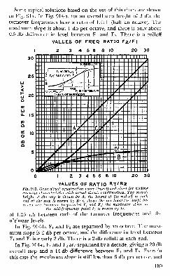
Some typical solutions based on the use of this chart are shown

in Fig. 914. In Fig. 914-a, for an overall step height of 3 db, the

turnover frequencies have a ratio of 1.4:1 (half an octave). Themaximum slope is about 1 db per octave, and there is only about

0.5-db difference in level between Fx and F2 . There is a rolloff

VALUES OF FREQ RATIO F2/F1

0 I 2 3 4 5 6 8 10 20 30

VALUES OF RATIO RT/R2Fig. 913. Generalized equalization curve (insert) and chart for finding

essential characteristics with actual circuit combinations. The overall

height of the step is shown by A; the height of the roll-off at each

end of the step is shown by B; C shows the net boost (or drop) be-

tween the turnover frequencies F, and F,; the maximum slope at

the mid-frequency point Fs is shown by D.

of 1.25 db between each of the turnover frequencies and the

ultimate levels.

In Fig. 914-b, F, and F2 are separated by an octave. The maxi-

mum slope is 2 db per octave, and the difference in level between

Fi and F2 is nearly 2 db. There is a 2-db rolloff at each end.

In Fig. 914-c, Fx and F2 are separated by a decade, giving a 20-db

overall step and a 14-db difference between F x and F 2 . Even in

this case the maximum slope is still less than 6 db per octave, and

189

the average slope over the 10-to-l frequency range is only 4.a db

per octave.

Terminal impedances

Now for the second source of error. If an equalizer designed

F l .5DB I.25DB 3DE

1 DB PER OCTAVE

f\ I.94DB 2.04 DB 6DB

2DB PER OCTAVE r 2

4.9 D B PER OCTAVE

vaaaMBaaiiaHjaHai

according to the methods in the preceding section is connected

between two existing amplifier stages, the results may not con-

form to expectations. The predicted response would be obtained

if the equalizer input voltage was the same at all frequencies.

Unfortunately, the input impedance changes with frequency, and

so does the voltage. The grid-circuit impedance of the following

stage also changes with frequency and affects the performance.

Fig. 915. The complete high-

frequency boost equalizer cir-

cuit containing the additional

elements affecting its character-

istics is shown in (a). In (b) is

shown the equivalent circuit ofthe source impedance used forfinding the low-frequency turn-

over point. The equivalent cir-

cuit for finding the high-fre-

quency turnover frequencypoint is shown in (c).

These plate and grid-circuit impedances must be included in the

design calculations for the equalizer.

Fig. 915-a is the basic circuit of Fig. 912-a modified to include

these source and output impedances. The low-end turnover

frequency is found by making the reactance of Ch equal to Rl.

The remaining resistance RT in the loop is now R2 in series with

the parallel combination of Rp (the plate resistance of VI) andthe load resistance RL (Fig. 915-b). As far as frequency discrimina-

tion is concerned, RT is the equivalent of R2 in Fig. 912-a. The

t

Fig. 916. Low-frequency-boost equalizer (a), andits equivalent input impedance (b).

high-frequency turnover F2 is found by making the reactance of

CH equal to the parallel combination of Rl and RT (Fig. 9 15-c).

In practice it will be necessary only to find one of these frequen-

cies. Fi is the easiest to calculate, and Fig. 913 gives all the other re-

lationships.

As an example, suppose that Rp is 1.5 megohms, RL is 330,000

ohms and R2 470,000 ohms. A high-frequency-boost step of 15 db

191

is required, starting at a low-frequency turnover of 2,000 cycles.

Rp in parallel with RL gives about 280,000 ohms net plate-circuit

resistance; this added to 470,000 ohms (R2) gives 750,000 ohmsfor Rt . A 15-db boost calls for a ratio R1/RT of 4.6 (curve A in

Fig. 913), so that R1 works out to about 3.5 megohms. A standard

value of 3.3 megohms would be close enough. The circuit will

show a boost of 2.9 db (curve B in Fig. 913) when Cn has a

reactance of 3.3 megohms at 2,000 cycles (25 ngf).

i

Fig. 917. A workable form of low-frequency-

boost equalizer, with the d.c. return to ground(a). Equivalent circuit derivation (b).

Now the grid-circuit impedance of V2 enters the picture. If the

input capacitance CG is 25 ppf, the total attenuation will be 6 db

more than anticipated, because Cn and CG form a 2-to-l capacitive

voltage divider at the highest frequencies. Using a smaller value

for R2 will reduce the effect of CG . With R2 equal to 100,000

ohms, Rt becomes 380,000 ohms. R1 then works out to 1.75 meg-

ohms (standard value 1.8 megohms). CH would then be 50 ggf for

a 2,000 cycle low-frequency turnover. With CG equal to 25 uui:

,the

added loss is only 3.5 db.

Increasing the overall height of the step will offset this loss still

further. Using a figure of 20 db, the ratio R1/RT will be 9. R1works out to 9 X 380,000, or about 3.3 megohms, which again

calls for CH = 25 ppf to lift at 2,000 cycles. The loss due to CG

will be 6 db, leaving a net step height of 20-6, or 14 db.

In any case it pays to reduce the V2 input capacitance to the

smallest possible value. One method is to develop a large amount

of inverse feedback in V2 by using an unbypassed cathode resistor

or by operating V2 as a cathode follower.

192

Bass-boost circuit

Let us turn to the bass-boost equalizer following the basic

circuit of Fig. 912-b. Input and output impedance factors are

shown in Fig. 916. Here R2 is in series with CL (Fig. 916-a) and

the balance of the circuit is the series-parallel combination shown

in Fig. 916-b. This circuit would not work in practice because

t

Fig. 918. Another form of low-frequency-boostequalizer (a). TO may be a variable resistor forcontrolling the response. The equivalent circuit

is given in (b).

the V2 grid circuit has no d.c. return to ground. Two workable

arrangements are shown in Figs. 917 and 918, and the

equivalent basic derivation is given under each. In Fig. 917, R3shunts all the other elements (R2 is effectively open-circuited by

CL). This is the simplest circuit to use. Fig. 918 is better where

adjustable boost is required.

In this case the simplest reduction to the basic form of Fig.

912-b is by using RT of Fig. 918-b as an equivalent for (R1 + R2)

,

and R2 and R3 in parallel as an equivalent for R2 of Fig. 912-b.

The equivalent of R1 can then be found by subtracting the

equivalent of R2 from that for (R1 -j- R2) . If R3 of the practical

circuit is nearly zero, both (R1 R2) and R2 of the basic circuit

are approximately equal to this R3, and R1 is effectively almost

zero. This shows that, as R3 approaches short-circuit, the step van-

ishes.

Turning back to the question of the errors arising from failure

to take circuit impedances into account, take the example shownin Fig. 919. This network is intended to boost both ends of the

frequency range. The values of R1 and R2 in the basic circuit

193

of Fig. 919-a should give a lift of about 14 db at each end. If this

arrangement is merely inserted between two stages, as in Fig.

919-b (ignoring for the moment the need for a d.c. grid return),

the plate-circuit impedance of VI will reduce the high-frequency

boost and increase the bass boost, throwing the whole arrange-

ment off balance. With the values shown, the plate-circuit resist-

ance is about 330,000 ohms. RT is 550,000 ohms, so the ratio

R1/R2 is only about 2, giving less than 10-db top lift (ignoring

possible effects due to input capacitance). For bass lift R1/RT

is about 6, giving nearly 16-db lift.

Fig. 919. A combination high-low-boost circuit.

The basic network appears in (a); with theinput and output circuits added (b). Compen-sation for equal high- and low-frequency boost

is provided by adding resistor R) (c).

By careful choice of values in the circuit of Fig. 919-c, using

the equivalents shown in Figs. 916 and 918, R3 will not affect

the top lift materially, but its value can be adjusted to bring the

bass boost to the required equal value. The values shown will give

14-db lift at each end. The reactances of capacitors CH and CL

must be equal to R1 and R2, respectively, at the high and lowturnover frequencies. To avoid confusion the effect of grid input

capacitance has been ignored; to include it, the procedure for

designing the top lift will be as in the earlier example, after whichthe bass lift can be adjusted by R3 as just stated.

194

scope test procedures

Magazine articles and textbooks often describe the use of scope

patterns to detect or assess amplifier distortion. The method,

theoretically, is simple. One merely connects the input of the

amplifier to the X plates and the output to the Y plates.

As generally presented in the literature, patterns show the

effect of either distortion or phase shift. In practice, however,

distortion and phase shift frequently come together, so that an

entirely different pattern is produced.

Fig. 1001 shows the general arrangement used for obtain-

ing these patterns. Without doubt, the method itself has advan-

tages over either examining a scope trace of input and outputwith an ordinary time base (with or without electronic switch-

ing) or analyzing input and output with a wave analyzer. For bothmethods, the input should be almost a perfect sine wave.

For this method perfection of waveform is not so important,

although the source should be at least ostensibly a sine wave.Compared with the viewing of waveform with an ordinary timebase, small degrees of distortion, particularly lower-order har-

monics, are easier to detect and identify.

The use of a wave analyzer identifies precisely the componentfrequencies produced by distortion but does not indicate howthese component frequencies add up to modify the waveform.To diagnose the cause of the distortion, the actual departure of

the waveform from its true shape is more helpful than a detailedanalysis of the harmonics introduced.

195

To make the whole matter quite clear, we will start by dis-

cussing phase-shift patterns when no distortion is present. Fig.

1002 shows three families of phase-shift ellipses. In each case zero

Fig. 1001 . The equipment hookup for di-

agnosing amplifier distortion with oscillo-

scope patterns. In using this arrangement,lower-order harmonic distortion is easily

detected and identified.

phase shift is indicated by a sloping line, which means that the

spot traverses to and fro along the same trace. Introduction of

phase shift opens the line out into an ellipse and, when 90° is

reached, the major and minor axes of the ellipse are horizontaland vertical. Beyond 90° the ellipse would tilt the opposite way,finishing up with a straight line sloping the opposite way for180° phase shift.

The three groups of Fig. 1002 help clarify the significance otthe mathematical properties of various ellipses. In the center

group the deflection due to the X and Y plates is equal, so the

zero phase-shift line is at an angle of 45°, and the 90° phase-shift

trace is a circle. The left and right groups of patterns show the

resulting pictures when the X deflection is less and greater, re-

spectively than the Y deflection. It is most convenient for diagnosis

to use the equal-deflection pattern shown in the center of Fig.

1002 if at all possible. In some instances this may not be easy

with the equipment available, so it is necessary to make out a

pattern on unequal X and Y deflections. Ellipses are shown for

10° intervals of phase shift from zero to 90°, and the 30° and

AF 0SC ATTEN »MPL

60° phase-shift ellipses are identified and distinguished from the

others by being drawn blacker.

Points by which to deduce the phase shift of any given ellipse

are marked on the figure. The best way to measure such an

Fig. 1004. Six examples of how a distorted trace’s shape varies with phase shift.

A full discussion of this is covered in the text.

ellipse is to place a transparent cursor with graph ruling in front

of the scope and adjust both deflections so as to fill an even

number of squares. This provides a handy reference. Consider

197

halt of one side of the square containing the pattern as equal

to the unit “1.” Using this graphical unit of distance, the loca-

tion of the points indicated (along the left and bottom edges) is

measured from the center or center line of the pattern.

Finding the phase angle

The point where the ellipse crosses the vertical or horizontal

center line, measured from the center of the pattern, is the sine of

the phase-shift angle. (For example, the 30° ellipse crosses the

line at 0.5 the length of the line.) The point on the boundary

square of the pattern where the ellipse touches it, measured along

that side from the center line, is the cosine of the phase-shift angle.

The cosine is measured as a decimal fraction of the line, and the

angle can then easily be found by reference to a simple table of

sines and cosines.

Fig. 1005. Diagram of a simple phase-shift

network. This arrangement affords continual

phase shift up to 30° either side of zero posi-

tion, and it is commonly used in many com-mercial test instruments.

It is naturally easier to use the sine reference for angles be-

tween zero and 45° and the cosine reference for angles between

45° and 90°, but it is a good idea to measure off both points as

a check, particularly where the angle lies between 30° and 60°.

It is also a good plan to take an average of all four possible read-

ing points for each value, to eliminate any error due to the ellipse

not being quite correctly centered in its boundary square.

Distortion

If the reader has tried to calibrate an oscillator with Lissajous

patterns (as described in Chapter 14), he will notice that when

the patterns are not quite locked they appear to be moving

around. The direction of movement is somewhat subjective; that

is, it depends upon the imagination of the viewer at the moment.

The movement could be imagined as being due to a pattern

traced on a transparent cylinder, which is rotated on its axis so

the pattern on the far side is viewed as if it were superimposed

on the pattern in front. The cylinder could equally well lie on

a horizontal or vertical axis, whereupon the movement due to its

apparent rotation will appear at right angles. If either of the

198

patterns has a slight distortion, particularly noticeable at one

point in the waveform, the direction of the axis of rotation seems

to be identified by the movement of this distortion point. For

example, if there is a little kink in the 60-cycle waveform due to

rectifier pulse current in a power-supply unit connected to the

same power line, this kink will maintain a regular position

horizontally, moving up and down along a vertical line in the

°UT

^y'

Fig. 1006. A three-frequency shift net-

work arrangement.

trace, and the kink will appear at all points in the pattern where

it crosses this vertical line. This will give the impression that

the pattern is moving up and down vertically or rotating on a

cylinder with a horizontal axis. On the other hand, if the output

from the oscillator has a similar definite distortion mark, the

apparent movement will be the opposite way, the distortion marktraveling along a definite horizontal line in the pattern as if the

rotation were due to the pattern being traced on a cylinder with a

vertical axis.

All this is perhaps a little easier to visualize with Lissajous pat-

terns where the frequencies applied to the two sets of plates dif-

fer. For our purpose the frequency applied to both sets of plates

is the same and the pattern does not move because the phase

difference remains constant. However, there are ways of makingthe pattern move by introducing phase shift deliberately, and this

can be an aid in recognizing the particular form of distortion.

Fig. 1003 shows that deliberate phase shift can be introduced

into the signal fed to the X plates or that to the Y plates. For

practical purposes it is best to introduce phase shift only into the

undistorted signal fed to the X plates, because a phase-shift net-

work will alter the shape of waveform distortion, making it harderto recognize.

199

Fig. 1004 shows the effect of phase shift applied in this way,

together with construction lines (representing our imaginary

cylinder) to help visualize the movement of the trace as phase

shift takes place. The pattern at B shows the trace due to simple

distortion with no phase shift. This distortion could be due to grid

current or similar action producing clipping. The bent thick line

can be regarded as an ellipse viewed edge-on, with the ends bent

over, rather like what might happen to the rim of a bicycle wheelif it fell into a slot in the paving and the rider fell off the bike side-

ways. The thin lines are construction lines to identify the position

of the sudden bends and can be regarded as intersecting circles

viewed edge-on.

The pattern shown at A is due to phase shift in the deflection

of the X plates, and C shows the effect of phase shift in the

deflection of the Y plates only.

The remaining patterns D, E and F show the effect of com-

bined phase shift on both sets of plates, maintaining the same

phase shift in the Y-plate deflection as that shown at C, which

means that the points on the actual trace will move along hori-

zontal lines as the X shift is varied. To aid in visualizing this,

horizontal lines are drawn for the points where the curve suddenly

changes, at C, D, E and F. To allow these points to move on a

path similar to a point on the surface of our imaginary vertical

cylinder, the original construction lines, becoming ellipses, movein the peculiar manner indicated at D, E and F. The arrows onthe ellipses indicate an imaginary direction of rotation consistent

with the arrows on the thick line showing direction of spot move-ment. This direction is arbitrary and might easily be in theopposite sense to the one shown.

At D the phase shift in both deflections is in opposite ways, so

the resulting pattern is more opened out. At E the two phaseshifts are the same way and the same amount, so, if no distortion

were present, the straight line, due to the equivalent ellipse beingviewed edge-on, would be restored; but the bent-over portionsare now moved round so they appear as loops moving away fromthis straight line. F shows the way the pattern distorts when theX phase shift is in the same direction as the Y shift, but bigger,so as to turn the pattern inside out.

Some of these variations may occur in practical amplifiers.

Phase shift may occur before the distortion sets in and furtherphase shift may be introduced after the point of distortion. If the

200

phase shift is due to the fact that the frequency of the signal is

either at the high or low end of the spectrum, it will be pro-

gressive, all in the same direction, as the signal goes through the

amplifier, before and after the point where distortion occurs. But

if viewed from the point of distortion, the earlier phase shift will

be in the opposite direction from the shift after that point (the

signal on the X plates will be in advance of the point of distortion

and that on the Y plates behind it in phase).

This combination would produce a pattern somewhat like that

shown at D in Fig. 1004. Phase shift only before or after the

distortion point would give an effect similar to the trace shown

at A or C respectively of Fig. 1004.

To aid in recognizing patterns due to practical amplifier distor-

tion, it may therefore be helpful to inject deliberate phase shift

into the signal fed to the X plates. Fig. 1005, shows a simple

circuit that will give continuous phase shift variation up to about30° either way from the zero position. The capacitors are markedin terms of their reactance at the frequency for which the net-

work is used. Of course, it can be used only at one frequency or

over a very limited range of frequencies, with any particular set

of values, but the arrangement could be modified by switching

in different capacitors to provide phase-shift facilities at different

preset frequencies. This type of network is used for phase shifting

in many test instruments.

Fig. 1006 shows the arrangement applied with switching for

frequencies of 100, 1,000 and 10,000 cycles. An extra switch is

provided so the phase shift network can be inserted or removedat will. This enables the frequency applied to the amplifier to

be swept through the frequency spectrum without deliberate phaseshift, switching over to the phase-shift arrangement at the preset

frequencies of 100, 1,000 and 10,000 cycles for more detailed in-

vestigation of the pattern at these points.

Fig. 1007 gives a complete set of prepared patterns for a

variety of typical defects in amplifier performance. The patternfor no phase shift is arranged in the second column from the left-

hand side for convenience—that for X phase shift only being to

the left and that for Y phase shift only to the right of it. Theremaining columns give the effect of equal X and Y phase shift of30°, the opposite way and the same way. The kind of defect givingrise to the distortion is noted down the left edge of the diagram.

The first four groups of patterns relate to clipping due to grid

201

current or similar action and curvature due to tube characteristics.

The former may be due to inadequate grid bias and the latter to

too much grid bias. Wrong plate loading can also cause these

troubles. Some of the patterns show little difference between the

two kinds of distortion. Notice where the X and Y phase shift are

the opposite way. Here the difference between the two kinds

of pattern is very small and would be difficult to identify on an

actual trace. This means that if some phase shift occurred before

distortion, with some more phase shift after it, it would be difficult

to determine which of these two kinds of distortion was taking

place. Introduction of phase shift in the X plates to neutralize

that in the amplifier before distortion occurs would produce a

pattern similar to that shown in Fig. 1007, in the column "Y phaseshift 30°,” where the difference between the two forms of distor-

tion is quite clearly identified.

If sufficient phase shift were introduced in the feed to the Xplates to offset all the phase shift in the amplifier, the trace wouldbe similar to that in the last column of Fig. 1007. Here again

the patterns are distinctly different. Probably the easiest point to

detect the difference is that where the trace divides. In the pattern

due to clipping, the curve splits abruptly, but in the pattern

due to curvature it forks apart smoothly.

The next line of patterns illustrates the kind of distortion due

to magnetizing current in a transformer core. For the previous

patterns it would be immaterial which kind of X phase shift

were introduced (by itself), because the pattern with no phase

shift has a kind of symmetry demonstrated by the fact that the

spot retraces its path to produce a single line trace. With this

kind of distortion, such symmetry cannot exist, so 30° phaseshift produces a different pattern, according to which way the

phase is shifted. One direction is indicated in the figure by the

solid line, and the opposite kind of phase shift, where it follows

a different course, by the dotted line.

Where the phase shift through an amplifier is progressive, as

at low frequency, the dotted-line pattern would be the one seen;

but where a similar phase shift is inserted in the deflection to the

X plates, the solid-line pattern would be produced. The effect of

phase shift after the point of distortion is shown in the “Y shift

30°” column and combinations of phase shifts in the remainingtwo columns.

Another kind of distortion that produces patterns somewhat

202

Fig. 1007. Some common forms of distortion resulting from different phase-shiftcombinations. These are patterns representative of a variety of typical defects to befound in unsatisfactory amplifier operation. The first three vertical columns are for10° X phase shift, 0 ° X and Y phase shift and 30° Y phase shift respectively. The last

two columns show the effects of combined 30° X and Y phase shift occurring first

in opposite directions and then in the same direction.

203

similar to transformer-core distortion in some phases occurs wnentubes in class-B operation are so badly matched that one tube cuts

off before the other starts to conduct. A variety of patterns for this

case is shown in the next line of the figure.

The last line illustrates the kind of pattern produced whenhigh-frequency ringing occurs in the drive transformer of an

output stage where positive excursions of the output tube grids

are encountered. The ringing is due to shock excitation of anultrasonic resonant frequency in the drive transformer circuit each

time grid current ceases.

204

speaker systems

Some points about the functioning of loudspeaker crossover

networks should be clarified. Most classical treatments derive

crossover networks from wave-filter theory which in turn is de-

rived from the theory of artificial lines (Chapter 9). The resulting

designs may not satisfy all the requirements of a crossover net-

work in the best possible way.

The first and most obvious requirement of a crossover network

is to deliver low-frequency energy to one speaker and high-fre-

quency energy to another. This is usually taken care of reason-

ably well, using a rolloff slope to suit the designer’s whim.A second factor (and one that often receives less attention) is

the impedance presented to the amplifier by the combined net-

work. Frequently this varies widely over the audio range and

includes sizable reactive components in the vicinity of the cross-

over frequency. To obtain best performance from the amplifier,

a constant resistive impedance should be presented to it as a

load.

The third requirement often receives even less attention. This

is the realism of the acoustic output from the combination. While

this is in some respects a matter of individual conditioning and

preference, it depends fundamentally on certain electroacoustic

requirements. One of the most important, and frequently the

one least considered, is the phasing or apparent source of the

sound output.

Tests have shown that phase distortion with single speakers is

205

not normally detectable; but when two sources are employed, the

phase relations between them influence the character of the

radiated sound field. The frequency response as registered by a

good pressure microphone may be flat, but what about the wave-

shapes? The pressure microphone does not answer that, but a pair

of human ears can detect such phase peculiarities. Failure to con-

sider this factor has made many dual-unit combinations sound

SPEAKERS CORRECTS PHASED SPEAKERS OUT OF PHASE

Fig. 1101. This diagram shows how the

apparent sound source shifts when speak-

ers are not in phase with each other as

compared to a condition where speakerphasing does exist.

noticeably unreal, even though their frequency response maylook perfect and there may be no measurable distortion.

Source of the sound

The reader may have checked two speakers for phasing by

listening to them while connections to one of them are reversed.

Standing some distance in front of them on the center line(as

in Fig. 1101) when they are correctly phased, the sound seems to

come from a point midway between the two units; but when in-

correctly phased, two effects can be noticed. There is a deficiency

of low frequencies (due to cancellation effects) and the source of

sound at higher frequencies no longer seems to be associated

with the units actually radiating it. This is because the air-particle

movement caused by the radiated sound is no longer back andforth along a line from the common source, but approximately at

right angles to it. The sound field around the listener’s head is

perpendicular to what it should be, causing, through our binaural

206

perception, the confused impression which may be called “dis-

sociation effect.” Further discussion on this will follow later in this

chapter.

A similar dissociation effect will occur with dual units driven

by a crossover system at any frequency where the two speakers

are out of phase. It is best to keep the two units close together.

Fig. 1102. Six examples of crossovernetworks for use with two-way loud-

speaker systems.

Some favor putting the smaller unit on the axis of the larger

one and immediately in front of it. But, however the units are

arranged, the dissociation effect can become noticeable if there

is an out-of-phase condition at some frequency near the crossover

point. The relative phase at crossover can be adjusted by posi-

tioning the diaphragms on their common axis so the wave fromthe low-frequency unit emerges in phase with that from the

high-frequency one. When the units are mounted side by side onthe same baffle, the sound should emerge in phase at the baffle

surface.

Constant-resistance networks

How does the crossover network affect the relative phase at

frequencies near crossover? This question often seems to beoverlooked, and neglecting it can cause the trouble just described.

Some networks, of the kind employing two or more reactances

207

for each unit, have values adjusted to give an accentuated fre-

quency rolloff. For example, the networks shown at Fig. 1102-c-d,

using the values given by the chart in Fig. 1103, are of the

constant-resistance type, giving a rolloff of 12 db per octave. Thephase difference between the outputs is always 180 degrees; butusing values designed for a sharper rolloff, the phase difference is

not the same. At frequencies near crossover, phase difference

changes rapidly. Some out-of-phase effect in the vicinity of the

crossover frequency is unavoidable unless a constant-resistance

type network is used. It is fortunate that this type takes care of

both the second and third requirements already mentioned.

The chart may be used to design any of the six types of crossover

network illustrated in Fig. 1102. Those at a and b give a rolloff

of 6 db per octave and a constant phase difference of 90°. Forbest results the positions of the two diaphragms should be adjusted

so the difference in their distances from the face of the baffle is

about one-quarter wavelength at the crossover frequency. Thephase difference will not be serious within the range where appre-

ciable energy is coming from both units.

The networks at c and d give a rolloff of 12 db per octave, anda constant phase difference of 180°, which means that reversingconnections to one unit will bring the phase right. The unitsshould be mounted so their diaphragms are in the same plane.

For cases where the frequency response of the units used re-

quires a rolloff steeper than 1 2 db per octave, the networks shownat e or / are recommended. These give a rolloff of 18 db peroctave, and a constant phase difference of 270°. This means thatmounting the diaphragms a quarter-wavelength apart at the cross-over frequency will give in-phase outputs by appropriate connec-tion.

All these networks are designed to present a constant, resistiveimpedance to the amplifier over the entire frequency range.

Impedance variations

One more point is often overlooked. The networks are de-

signed on the theory that they are feeding resistance loads of the

same value as the nominal voice-coil impedance. The voice-coil

impedance is not pure resistance, so the performance of the net-

works is altered. The most serious effect is usually due to the

inductance of the low-frequency unit voice coil. By using net-

works a, d or e, each of which feeds the low-frequency unit through

208

CAPACITOR

VALUES

Fig. 1103. This chart is for finding the exact values of inductance and capacitance for any of

the networks shown in Fig. 1102- Use of the chart is illustrated in Fig. 1104.

:o9

IMPEDANCE

a series inductance, this effect can be overcome by subtracting the

voice-coil inductance value from the network inductance value

derived from the chart. Even if the available data are insufficient

to allow this, these networks will minimize the effect, because

the inductance of the voice coil will add very little to the effec-

tive inductance of the network. In the other networks the shuntcapacitor combined with the voice-coil inductance will cause a

greater variation in input impedance.

Each diagram in Fig. 1102 has the inductors and capacitors

marked with symbols. These identify the reference line (in the

bottom part of the design chart) to be used for finding each com-

ponent’s value. Fig. 1104 illustrates the use of the chart to find

values for a network of the type in Fig. 1102-e, and Fig. 1105

shows the actual circuit calculated in this way for a crossover fre-

quency of 500 cycles at 40-ohm impedance.

The input impedance is the same as each speaker voice-coil

impedance. Some prefer to design the crossover network for 500-

210

ohm impedance and use matching transformers at the outputs to

feed the individual voice coils. This method has two advantages.

The two units need not have the same voice-coil impedance and

smaller capacitors can be used. The range of impedances covered

by the chart extends up to 500 ohms to include such designs.

One modern trend has been to use separate amplifier channels

for each unit. In this case the chart can be used for designing an

Fig. 1105. The crossover-network com->onent values for the circuit of Fig.

1 02 -e as derived by the method shownin Fig. 1104.

interstage filter to separate the channels by making the following

adjustments. 1. Multiply all impedance values by 1,000. (This

means the impedance used to terminate each output is a grid

shunt). 2. Change inductance values to henries instead of milli-

henries. 3. Divide capacitor values by 1,000. Suitable networks

for this application are a, c or e, since these allow the input to

each amplifier circuit to be grounded on one side.

Dissociation effect and directional sensitivity

Undoubtedly many people have recognized the phenomenoncalled “dissociation effect” without fully understanding its

mechanism.

To understand the behavior of sound waves we must have the

relative wavelengths of audio frequencies clearly in mind. Acous-

tic waves travel approximately 1,100 feet per second in free air

so the length of one wave at a frequency of 1,000 cycles is a little

over 1 foot. Lower frequencies have longer waves, while the wave-lengths at higher frequencies are shorter.

Next we must see how it is possible for us, equipped with only

two ears, to determine the direction from which a sound origi-

nates. A single ear can give only a limited sense of direction be-

cause the spiral communicating channel between the outer ear

and the mechanism of the inner ear eliminates the external direc-

tivity. Directional sensitivity must be a function of the inter-

preting faculty of the brain derived by comparing the nerveimpulses received from both ears. This fact was stated at thebeginning of this chapter.

9.5MH TO HF UNIT

* 10.7 TO LF UNIT

211

Is this ability to discriminate based on the intensity relation-

ship or on the phase relationship between the two ears? The dif-

ference in intensity between sounds reaching the two ears from a

given direction in free space depends on the obstructing effect

(diffraction) of the head. This effect increases with frequency, so

the intensity on one side is greater at high frequencies than at

Fig. 1106 . A generalized diagram of the movement of the air particles arounda speaker.

low. The phase difference is also greater at high frequencies, be-

cause low-frequency waves are much longer than high-frequency

waves and change less in the short interval between their times of

arrival at the two ears. The fact that we are more sensitive to the

direction of origin of sounds at higher frequencies can be ex-

plained by either the intensity-difference or the phase-difference

212

theory. Our subconscious probably utilizes both effects to some

degree, but the dissociation effect makes it quite evident that the

phase relationship between sounds received by our two ears is the

more important of the two.

To prove this, we need to understand a little more about sound

SPKRS STAGE SPURS

UUUUUUUJX) UJjLUUUuuu

Fig. 1107. The plan of an auditorium thatpresented a serious problem in acoustics.

Proper speaker phasing arrangements wasthe solution.

waves and their propagation. It is well known that a cone loud-

speaker working without any kind of baffle or cabinet loses its

effectiveness at low frequencies because air escapes around the

edge of the cone. (When the cone is moving forward

,

air particles

around the rim rush backward into the partial vacuum behindthe speaker.) But what happens to other air particles farther

away from the speaker?

Fig. 1106 is a diagram of air-particle movement (somewhat

213

exaggerated) at various points surrounding the speaker. Particles

along the cone axis move back and forth along straight lines radi-

ating from the source. On either side of the axis the particles

spin elliptical paths which grow shorter and narrower as the

distance from the speaker increases. At extreme distances these

ellipses flatten to straight lines which also radiate from the center

of the cone. Note, however, that at points along the plane of the

cone the particles move at right angles to the radius line, so that

the sound at these points seems to come from left and right

instead of from directly in front of the listener. (Under ideal con-

ditions, the sound waves from left and right would cancel, so that

no sound would be heard along the plane of the cone.)

How does this affect our sense of direction? Try listening to a

speaker from different positions. You will find that anywhere—except for a small region near the plane of the cone—the source

of sound is easily identifiable with the speaker unit. In the plane

of the cone, however, the dissociation effect becomes noticeable

and it is almost impossible to say where the sound comes from.

When the dissociation effect is greatest, you get the impression

that, instead of having a single speaker unit in front of you , there

are two similar units, one on each side.

Phasing in PA work

Having investigated the matter so far, we can ask the question,

“Is speaker phasing important for public address or sound rein-

forcement work?” The answer is definitely yes. One particular

job is recalled where phasing played an important part. Fig. 1107

shows the layout of the installation. The auditorium was a long,

narrow rectangle, with the stage at one end. The only points

where speakers could be mounted were at the sides of the stage

and immediately above it, at the ends of the narrow sections of

the gallery. An engineer who did not realize the possible conse-

quences had simply connected the four speakers in parallel with-

out regard to phasing. The hall was acoustically poor due to a

natural echo, but it was symmetrical and he could not under-

stand why it was extra bad at certain spots especially along the

right-hand side. We suggested that two of the speakers be dis-

connected and observations of the type described above be con-

ducted on the center line. Similar tests were then made with the

other speaker pair. We found that one speaker on the right-hand

side had been connected out of phase with the other three. Re-

214

versing the offending speaker not only improved the bad spots

but made listening considerably better everywhere at the back of

the hall. The natural echoes were still evident, but not to such

a degree as to render sound almost unintelligible. The incor-

rectly phased speaker had introduced some echo effects of its own.

Fig. 1108. An example of another speakerlayout arrangement that requires special

phasing techniques.

which made listening even more difficult except where the listener

was comparatively close to one speaker unit.

Extended investigation on other installations has shown that it

always pays to check speaker phasing. It may be thought that

where speakers are arranged as in Fig. 1108, correct phasing be-

tween symmetrical pairs would be important, but not between

215

other units at different distances from the front of the hall. Tests

show that there is one really effective method of connection andthis is invariably with correct phasing. The explanation seems

to be that when a listener hears sound from two sources, one of

which is nearer than the other, as must happen in some positions

with an installation of this type, the nearer souce gives the im-

.a. .a. .a.

Fig. 1109. Side-by-side speakers can createproblems unless they are correctly phased.

pression of a direct sound, while the sound from the more distant

source is like an echo. Where the echo arrives long enough after

the direct sound to be distinguishable from it, phasing is unim-

portant; but there are always some positions where the twosounds arrive so close together that the ear cannot distinguish

them as separate sounds. At such positions, phasing can makean important difference.

Another type of installation is shown in Fig. 1109. Correct

phasing is very important here. Walk around the back of the

room while sound is being broadcast: When nearer to one speaker

the sound seems to come from the vicinity of this speaker. At a

point equidistant from two speakers, if the two are in phase, the

apparent source of sound seems to pass smoothly from one speakerto the other; but if they are incorrectly phased, there will be anarea of confused sound where the building echo seems empha-sized, often to the point of unintelligibility.

Crossovers

As previously mentioned, dissociation effect can also occur with

dual speaker units fed from an electrical crossover network, but

the effect is slightly different from the examples just considered.

You get the impression that one part of the frequency spectrumhas a source different from the remainder of the spectrum. In

large dual-speaker installations, such as in movie theaters, this

dissociation effect will be swamped by the natural reverberationof the auditorium. However, the effect can be quite disconcerting

216

in home equipment, giving the sound an unnatural quality that

many listeners have complained of.

Fig. 1110 shows two typical loudspeaker crossover networks, and

Fig. 1 1 11gives their phase characteristics. Although the two net-

works have identical schematic configurations, the one shown in

Fig. 1110-a has values chosen to provide constant resistance, while

the network of Fig. 1110-b uses typical wave-filter-derived values.

« t

Fig. 1110. Two identical speaker crossovernetwork configurations. The circuit in (a)

has values chosen to provide constantresistance, while the circuit in (b) uses

typical wave-filter derived values.

To make the distinction between the two types clearer, componentvalues have been marked in terms of their reactances at the cross-

over frequency, X 0 being a reactance equal to the characteristic

impedance at the crossover point.

The top and center A curves in Fig. 1111 show the phase

responses of the high- and low-frequency sections of the constant*

resistance type network. These have a constant phase difference

of 270° over the entire frequency range, as indicated by the solid

line A at the bottom. On the other hand, the high- and low-fre-

quency sections of the wave-filter-derived network have a phasedifference of 270° only at the extreme limits of the frequencyrange, while the difference between them increases to almost 450°

at the crossover frequency (curve B at the bottom).

With this type of crossover network, no matter how the h.f. andl.f. units are connected in an attempt to maintain constant phase

difference between them at or near the crossover frequency, there

will always be a rapid deviation from the constant-difference con-

dition near the crossover point. As a result, some component fre-

quencies of the reproduced sound will have their apparent sources

shifted to one side or the other away from the general apparentsource of the speaker combination.

If we are trying to reproduce a musical tone which contains a

series of harmonics extending through the crossover frequency,

217

this type of network will move the apparent sources of some of

the harmonics to positions a small distance away from the com-

mon source of the others.

It is perhaps well in concluding this chapter to emphasize one

point of phase difference that seems to have caused some con-

fusion heretofore. In electrical circuits, phase difference is essen-

tially a time difference, measured in degrees over the duration of

Fig. 1111. Graph showing crossover-network phase relations. Curves A are for

constant-resistance networks; curves B are for wave-filter types. Top and center

curves show high- and low-frequency shifts, respectively; curves at the bottom showthe phase differences between high- and low-frequency units over the entire range.

one cycle at the frequency considered. The acoustic effect on

which our ears base their directional deductions is better under-

stood as the slope of the wave in space at any particular instant in

time, and is thus a kind of spatial phase difference. This distinc-

tion may help some who find it difficult to see why two inter-

acting acoustic fields which differ in phase can produce effects

noticeable to the ear, even though electrical phase differences of

much greater extent are not normally detectable.

218

chapter

12

advanced techniques

I

t has been said, on both sides of the Atlantic, that the British

appear to lead the audio field. When asked to gather material

on British audio circuit features, we naturally asked ourselves the

question: Why do the British lead in this field? In what does this

leadership consist? Is it more advanced know-how, or is it just

doing an ordinary job a little better?

The consensus is that there is nothing particularly clever about

their circuitry in most instances. Rather, it is that more time

and effort is put into getting the best out of well-tried circuits or

their variations. Until recently, there was very little interest in

audio. American production-minded concerns did not find it

attractively profitable to invest in research for such small volume.However, some British outfits, working on a smaller scale, foundthe outlay worth while.

The market is growing with the widening interest, and it maybe that American concerns who manufacture in large quantities

will soon take the lead from the smaller British firms. However,it is probable that the latter will hold their own, for, even withthe market bigger, it will remain essentially an individualistic one.Audio enthusiasts are connoisseurs, and ears, like palates, vary.

So there should continue to be room for everybody who is pre-

pared to do a really good job.

Probably the connoisseur aspect of the audiophile is best evi-

denced in the variety of circuits for quality control, tone compen-sation or whatever name you like to give it Recently, we ques-

219

tioned a statement to the effect that bass boost and treble cut have

the same effect, and vice versa. We were immediately shownhigher authority for this opinion. The truth would appear to bethat the difference is indistinguishable to some, while to the more

discriminating ear the finer details of frequency response require

some control to obtain a satisfying effect.

Most modern audio equipment incorporates the control fea-

tures in a preamplifier remote from the main amplifier. An excep-

tion to this is a unit made by Telrad Electronics — and to pro-

duce many of the advantages of more expensive contemporaries

the whole amplifier is carried on one chassis. The controls are

remote and are connected to the main chassis by a relatively short

220

length of multiconductor cable, terminated in an octal plug. Fig.

1201 shows the remote panel circuit for this requirement. The tone

correction circuit is between the first and second stages, and the

volume control between the second and third. The circuit consists

JI liU\ __I Hr

IIill

B0

|i

tf'

-io jjf 7y In

In

M-100 200 300 *

10 — 1ft*

- 20

Fig. 1202. Graph shows the curves for six

control positions of Fig. 1201.

of a basic voltage divider, R1 and R2, which provides an attenua-

tion of about 26 db. Both bass and treble controls provide a level

position (as shown), three lifts and two cuts. The boost gives an

ultimate lift at either end of about 26 db. The position of the lift

Fig. 1203. Feedback circuit arrangement for input compensation in

the Leak “ Vari-slope” unit.

is varied by altering the capacitor values. Similar change of values

alters the two possible cutoffs provided for each end. The com-

bined range of control provided is shown at Fig. 1202. This ar-

rangement provides sufficient variation to satisfy all practical qual-

ity compensation required and has an advantage in that the differ-

ence between steps is perceptible.

221

Preamplifiers of more conventional type generally provide

somewhat wider facilities. The Leak Vari-slope1 separates the func-

tion of compensating for recording characteristic, etc., from the

compensation for studio or room acoustics and noise content, by

adjustment of bass and treble controls. The input selector switch

has five positions, marked radio, 78a, 78b, l.p. and mic. This com-pensation is achieved by a feedback arrangement over the first

stage of the preamplifier, as shown in Fig. 1203.

Over the second stage, the bass boost positions are achieved by

different values of series capacitor in the feedback. The cut posi-

tions insert different values of series capacitor in the lead to the

output volume control. (The combined bass control is shown at

Fig. 1204.)

The treble lift is conventional, but the cut positions employ the

Vari-slope technique from which the unit gets its name. Three

turnover frequencies are provided by the switch. At each, a con-

ventional two-stage rolloff response is provided between the first

and second amplifier stages. Combined with this is a further cor-

rection introduced into the feedback over the second stage, using

a form of adjustable twin-T network. Capacitor values are selected

by switch to suit the turnover frequency chosen. Variation of the

slope control shunts the T to varying degree, thereby changing

the shape of correction applied at the rolloff frequency. Thus turn-

over frequencies are selected in steps, but the rate of cutoff can be

adjusted continuously. Fig. 1206 shows a range of possible slopes

for the lowest cutoff, 5 kc. Fig. 1205 shows the basic circuit for

i Manufactured by H. J. Leak & Co. Ltd.

treble control, leaving out the components that affect only bass re-

sponse and the muting arrangements. Muting consists, quite sim-

ply, of shunting the switch contacts with suitable high-value re-

sistors to prevent residual charges being left on capacitors not in

use, so that switching them into use would produce a click.

Finally, one other circuit is that of the QUAD quality-con-

trol unit2. A particular feature of this unit is the mechanical ar-

rangement of the panel facilitating touch control. The volume

control employs negative feedback over the second stage, using the

circuit shown in Fig. 1207. At minimum volume, the second stage

operates at unity gain with 100% feedback, or nearly so, while at

maximum volume the feedback is considerably reduced.

Tone compensation is again divided into two parts, but the

functions are not separated in quite the same way as in the Leak

unit. Two different input sockets arrange for flat response or cor-

rection for velocity type pickups. The main compensation is in the

output circuit. This consists first of a filter with variable slope

characteristics, but using a conventional filter circuit modified for

this purpose, as shown in Fig. 1208. Two turnover frequencies are

available by switching capacitor values, at each of which the slope

can be varied very much like the “cut” part of the Leak treble

control. Following the filter in the circuit arrangement are the

fairly conventional treble and bass controls, as in Fig. 1209,

2 Manufactured by Acoustical Manufacturing Co. Ltd.

223

giving the response variation of Fig. 1210. In the panel arrange-

ment the physical position of the controls is reversed, as this is con-

sidered more logical from the psychological viewpoint.

Fig. 1206. Graph of the curves repre-senting the possible slopes for 5-kc cutoff.

The filter switch has four positions:

1 . Flat, cutting out filter and top and bass circuits, so that a

check can quickly be made against level response at any

time.

2. Bringing in treble and bass controls only.

3-4. Different filter turnovers.

Fig. 1207. Arrangement showing how feedbackis employed in the QUAD volume control

circuit.

There you are. Three completely different ways of doing vir-

tually the same thing. Each does its job well because of the work

that has gone into getting the right circuit values for the purpose,

rather than because its circuit is so much better than its competi-

tors.

The grounded grid

Turning from circuit practices in audio to future possible de-

224

velopments, let us look at the grounded-grid amplifier which is

familiar to designers who work at very high frequencies where it

is used for the final stages of transmitters in the kilowatt class and

in some wideband low-noise-level amplifiers. The audio designers

tig. 1208. Circuit of the basic filter used mthe QUAD unit.

have ignored its potentialities, both in America, where they call

it grounded grid, and in Britain, where they call it the inverted

amplifier. A while ago we began to wonder about using grounded-

grid stages in audio amplifiers. Setting their assistant to work, the

authors settled down and

. . wrote with a pen in each hand,

And explained all the while in a popular style

Which the reader could well understand.”

The experimental work which we completed had been carried

out with a 12AT7 double triode. This is not exactly a power tube:

Fig. 1209. The QUAD unit bass andtreble control circuits.

with plate supplies of 150 volts and a normal circuit you would

not expect to get 100 milliwatts of power from one triode section.

However, this happens to be just the sort of power needed for a

particular amplifier and offers the opportunity to try out the

grounded-grid stage with some feedback circuits which do not

seem to be in the books. The interested reader can apply the

theory to power amplifiers with the knowledge that he is on fairly

new ground.

First of all, what is the grounded-grid amplifier? The basic cir-

225

cuit is shown in Fig. 1211, where, as you can see, the input is ap-

plied between cathode and ground and the output is taken be-

tween plate and ground; the grid itself is connected directly to

ground. Bias is provided in the usual way by the voltage drop in

the cathode lead, and the input transformer can be dimensioned

to provide the necessary secondary resistance. It is instructive to

compare the three ordinary ways of connecting a triode amplifier:

grounded cathode, grounded grid and grounded plate. These are

drawn in Fig. 1212. They are three of the six possible ways of

using the triode. The complete set of six connections is shownsymbolically in Fig. 1213.

Fig. 1211. The grounded-grid amplifier. Thiscircuit is better known in the u.h.f. spectrum

than in audio frequencies.

The three elements of the tube are shown as terminals, with

signal being applied and output taken as indicated by the arrows.

An inward pointing arrow is input, and one pointing out is out-

put. Thus, at a the signal is applied between grid and cathode andthe output taken off between plate and cathode, as at a in Fig.

1212. Of these, a, b and c are already shown in Fig. 1212; d and e

appear to be quite useless and / has been used for measuring highvoltages. Negative plate voltages control the grid current with the

226

grid held positive, the tube having an amplification factor of 1/p.

Circuit features

The particular features of the grounded-grid amplifier, as weshall see, are low input impedance, normal output impedance andthe fact that the power which must be applied to the input is

Fig. 1212. The three practical ways in which an amplifier can be hooked up;(a) with cathode grounded, (b) with grid grounded and (c) with plate

grounded.

passed through the tube and mostly appears in the load. Let us

see how these features are produced. The equivalent circuit is

shown in Fig. 1214: e is the input generator voltage, acting

through an impedance R x , which includes any cathode resistor; pand RP are the usual tube parameters and R2 is the load resistance.

Fig. 1213. Six ways of hooking up a triodeshown symbolically. Setups (d) and (e) areimpractical; (f) is used only in special cir-

cuits. Fig. 1212 shows (a), (b) and (c).

*o c_P UoP *oT>P MoP «otoP «o oP

<t ( c 4 e f

The current i through the circuit is given by the equation:

e ~Heg

Ri -f- Rp -j— Ro (100

)

Now e g is the grid-cathode voltage, which is equal to iRi - e.

Therefore, by substituting for eg in equation (100), we get:

e - piRi + pe1 - R2 _p Rp _j_ R„

Rearranging this form gives

(101

)

e(l + p) =i[(l + p)R1 + RP + R2] (102)

The output voltage is, of course, iR2 , so that the voltage gain is

A y R, — 1 ^ t—e

A - —(1 + p)Ri + RP + R,

or,

A — _J_ y R 0+F)R2-e

A ‘'

(1 + p)Ri + RP + R2

X r2 (103)

227

If you remember the expression for the gain of the ordinary

grounded-cathode amplifier as A = gR2/[RP + R2 + (g + 1) Ri,]

you will see that, when there is no cathode impedance, the

grounded-grid stage gives the same voltage gain for a tube with

an amplification factor g as a grounded cathode stage with a tube

of amplification factor 1 + g. Using a cathode resistor the term

(1 -f- g)Ri appears in both cases.

The input impedance of the grounded-grid stage is quite easy

to calculate. It is

Rln = 4- = R, +R,

i

+ ^(104)

For the grounded cathode stage, as you know, the input impe-

dance is theoretically infinite. This input impedance may be sim-

plified a bit to give an approximate value which is easier to re-

member. Since we always use triodes in the grounded-grid stages,

R2 = RP . We have then:

R,„ - Ri2RP

1 + g+ 2^- ~ R, + 4g gn

(105)

where gm is the tube transconductance. For most of the tubes we

are using nowadays gm = 2,000-10,000 gmhos, so that l/gm maybe of the order of 250 ohms and Rln = Ri + 500 ohms. Let us take

Rj = 500 ohms, and we have Ri„ = 1,000 ohms.

For a small tube, a drive of 4 volts may be needed: the resulting

power input is 16 milliwatts. This drives a current of 4 ma

through the circuit, producing a power output in 10,000 ohms,

again a typical value, of 160 milliwatts. If we scale up these figures,

you see that a driver stage for a 16-watt grounded-grid amplifier

must deliver 1.6 watts: this is quite a contrast with the ordinary

power stage which needs only a few milliwatts.

The output impedance is most easily calculated by remember-

ing that if the output is matched it will produce one-half the open-

circuit voltage. Since the open-circuit gain, obtained by letting

R2 -» oo , is 1 + g, the output impedance equals the value of R2

for which the gain is:

, (1 +g)R2 _ 1 + g

R2 Rp + (1 + g)Ri 2

This gives for the output impedance the not unexpected value

Ro = RP -f- (1 + g)Ri- Since the (1 + g)Ri term is of the nature

of a negative feedback, the optimum load is, not the matching

228

load, but the load settled by the tube characteristics and is about

RP .

Before we go any further, let us summarize the results:

1.

Gain:

A - (1 +h)R3

R2 + Rp + (i + p) Ri

2.

Input impedance:

Rjn -—• Ri -f-

Rp + R2

l+P

3.

Output impedance:

Rnu t= Rp + (1 + lt)Ri

Notice also that the output is in phase with the input: the 180°

phase shift of the grounded-cathode stage is not obtained with

grounded grid or grounded plate (cathode follower).

Applications

At this point you may ask why the grounded-grid stage should

be used at all: the only important feature seems to be that it needs

a lot of power to drive it. The answer is that it is very easy to drive

it into grid current because of the low-impedance grid path, and

in consequence a triode can be driven over a much bigger plate

swing. A 12AT7 may operate linearly up to eg = +3 volts, instead

of being limited to the negative grid voltage region. Just what

this means can be seen by looking at the tube characteristics shown

in Fig. 1215: the positive grid characteristics were taken on a

cathode-ray oscilloscope and are thus not very exact, but in view

of the large tolerances which are normal for tube characteristics

this is not particularly important.

If we consider the probable working range of the 12AT7 with

positive grid drive, we see that, instead of working through the

point A (Fig. 1215) with a load of 15,000 ohms, we can workthrough B with a load of 5,000 ohms. For the first case we get a

peak voltage of about 401 and the maximum power will then be

(40)2/2 X 15,000 = 53 milliwatts. For the second, peak voltage is

50 and maximum power is about (50)2/2 X 5,000 = 250 mw.

The actual power drawn from the plate supply increases, in this

example, from 120 v X 4 ma = 0.48 watt to 120 v X 10 ma = 1.2

watt, but the efficiency is doubled. The audio designer who be-

lieves in triodes at all costs (and there are still quite a lot of peo-

229

pie who distrust the pentode and tetrode) thus has a chance of

getting more reasonable efficiency from his triodes.

The input impedance is made up of the cathode resistance and

a term (Rp + R2)/(l + g) which, when the tube is matched, is

simply equal to 2/gm . It is easy to see from Fig. 1215 that gm in the

working region is about 6,000 pmhos, so that 2/gm = 330 ohms.

To obtain an output of 50 volts peak with a gain of 1 + (fi/2) =31/2 requires a drive of 50 -5- 31/2 = 3.2 volts. The input power

Fig. 1214. The equivalent circuit of the

grounded-grid amplifier.

needed to give our theoretical 250 mw is thus, neglecting grid

current, 3.22/ 2 X 330 = 15.4 mw. Grid current will amount to

about 2-ma extra current to be provided at the peak cathode cur-

rent, and this will bring the input power needed by the grounded-

grid stage appreciably above the maximum power we can get from

a conventional grounded-cathode circuit.

In practice we have found the limitations of the driver result in

a maximum output power of about 200 milliwatts. The power

gain obtained from a complete 12AT7, with transformers de-

signed for the same input and output impedance and covering the

usual audio band, is about 50 db.

Positive feedback

Since the first half of a 12AT7 will not give enough power to

drive the second half fully, we are in rather a spot. The solution

is to make the second half, the grounded-grid stage, help drive it-

self. This we can do by means of our old friend positive feedback.

What happens if we apply feedback to the grid of a grounded-grid

stage? You will not, we think, find the answer in the textbooks,

and so you must bear with just a little more mathematics. We go

to our first equation, e - peg = i (Ri + RP -f R2), and now we say

that to eg we will add a fraction of the plate voltage /?iR2 so that:

eg = iRx — e + 0iR2 (106)

230

Substituting this in the original formula (equation 100), wenow have:

e(l + |i) = i[(l + 11 ) Ri + RP + (1 + [x/3)R2] (107)

From this we can see the following relationships;

1. Voltage amplification:

(i + f)R2A' —e (i + i*)Ri + Rp + (i + p^)Ra

Input impedance:

Rp I +W8Rin = 4- = Rj + + 1+P

Ro

(108)

(109)1 + p

3. Output impedance:

= (1 + jx)Ri + Rp

1 + y '

The amount of feedback is defined by the factor /?. If /? is posi-

tive, the feedback is negative, while a negative value of /? cor-

3~T—

/ +2

/ '

/_is X 0 E

// W< B

// s X -2

ft*' 3^.-520 40 60 80 KM 120 140 160 180 200

Ea VOlTS

Fig. 1215. This graph shows howthe grounded-grid circuit can berun into the positive grid region.

responds to positive feedback. For use in our amplifier the choice

of /? = — 1 /u is of special interest. This value of positive feedback

gives

A' - (] + lOR*

(1 -f- p)Ri + Rp (111

)

where the input impedance = Rx + (Rp/1 + p), and output im-

pedance = oo (infinity).

If we leave out the cathode resistor Ri we see that the voltage

gain is doubled by using this amount of positive feedback andtaking a load resistance R2 equal to RP . At the same time the input

impedance is reduced to 1 /gm instead of 2/gm . Consequently we

231

need only one-half of the previous driving power. This brings us

very nicely into the range of the grounded-cathode driver stage.

The way is thus cleared for the design of a simple audio amplifier.

The circuit diagram appears in Fig. 1216.

The output transformer T3 has three windings: the main wind-

ings are designed to suit the load, which we shall take to be a 500-

ohm line for design purposes. The optimum plate load is 5,000

I2AT7

ohms, from Fig. 1215, so that the turns ratio will be y/5;000/500

= 3.16:1. The stepdown from the plate winding to the grid is to

be 1 /\i, which is 40:1. If we want the amplifier to have a response

extending below 100 cycles, we can take a line inductance of 1

henry, which would give a 3-db drop at 80 cycles. The other in-

ductances are then 10 henries for the plate winding and 10/ (40)2

= 6 mh for the grid winding. This last winding must have low

resistance, so as not to cause a voltage drop when grid current

flows, but there will not be much trouble with such a low induct-

ance. The interstage transformer must match the ordinary class-A

stage to the cathode circuit, and must therefore have a ratio of

VI 5,000/1 60) or about 10:1.

Including an interstage transformer makes it fairly straight-

forward to add negative feedback either from the output plate it-

self or from the line side of the output transformer. There are dif-

ficulties in practice, of course, especially if you want to take the

feedback from the line winding, because then there are two trans-

formers in the loop, and the resulting 24 db/octave slope of the

232

total ultimate cutoff means you must stagger the cutoffs rather

well. If the feedback is taken from the plate, the shunt capacitor

shown in Fig. 1216 will help supply the needed stability.

The outline of the simple 12AT7 amplifier will, we hope, help

you to design something more powerful. The sort of amplifier

most readers will find interesting is probably a booster unit to

tack on behind an existing power amplifier. This is how the radio-

a

Fig. 1217. The negative-resistance circuit (a) and its

equivalent form (b).

frequency designers use the grounded grid: They take a 300-watt

transmitter and add a 1-kw stage, and then a 3-kw stage, and so on.

If you have a 3-watt audio amplifier, you can use this as a driver

for a 10-watt grounded-grid stage: the low impedance output of

your present 3-watt amplifier will probably give enough volts to

drive the grounded grid input, and it is easy to check this in the

tube characteristics.

Negative resistance

We bypassed this aspect of grounded-grid use temporarily, in

order to have space to look at some other consequences of the

equations. As we saw earlier, with positive feedback of p = -1 /pthe output impedance is infinite. The general equation for the in-

put impedance (equation 109), reduces, if Rt = 0 and R2 = Rp,

to:

Rin = -* + R„ (112)1 + g

By taking j3 = —2/p we make the input impedance zero. At the

same time the gain becomes infinite. This is therefore another

important value of positive feedback: any more feedback will

make the input impedance negative.

A further interesting value of /? is ft= -1 . This makes the in-

put impedance:

Rin Ri +R

+1 -

1*

1 + pR2 (113)

1 + F

233

Since p is usually fairly large — for the 12AT7 it is about 40-60

—consequently (1 - p)/ (1 -f- p) ss - 1 and the input impedance is:

Rin = Rl +1 +% Ra

As Ro is about the same order as RP, the term RP/1 -f- p does not

have much effect on the negative impedance. It is not very difficult

Fig. 1218. This push-pull negative-resistance circuit canbe used as an oscillator or a high-gain amplifier.

to show that if p changes by 10%, the term (1 — p)/(l + p)

changes by 2/1600 of 10%. The circuit thus provides a very stable

sort of negative resistance. Before explaining how to use this, weshall show how we actually obtain it. The essence of the circuit is

shown in Fig. 1217-a, in which a 1:1 transformer (a center-tapped

choke) provides the phase reversal to make /? = -1. The R-C cir-

cuit in the grid is just to keep the plate-supply voltage away from

the grid. The equivalent circuit is shown in Fig. 1217-b. Nowadayswe usually seem to get two small triodes in every bottle, so we can

elaborate Fig. 1217 into Fig. 1218, a push-pull version of the samecircuit. For audio work, we can have R4 = 10,000 ohms and R3 =1 megohm. C4 is chosen to produce a cutoff in the region of 200cycles, say .001 pf, while C3 provides a top cutoff, which may be at

5 kc, and then C3 will be .003 pf. At frequencies in the middle of

the band, when C4 can be taken as a short circuit and C3 as anopen circuit, ft = —0.99. The input impedance then has a value of2RP/(1 + p) — (R2/n2

).

Without going into too many details, it is sufficient to say that

the value of n is chosen in the same way as if the transformer wasto work into a resistance of R2 , and R2 should be about 10,000

—

15,000 ohms for a 12AT7 tube.

What is the object of producing this negative resistance? Thereare three sorts of job for which negative resistance is useful. It can

be used with a tank circuit to provide an oscillator; in a filter to

234

improve the Q of a coil or in a special type of amplifier circuit.

This last reference is the application for which the circuit of Fig.

1218 is of special value. Consider the very simple circuit of Fig.

1219. A generator of impedance R0 is connected to a load Rothrough a negative resistance -R. The current is;

.e

1 —2R0 (

- R)

and the voltage across the load will be:

eR0e° - 2R0 (

- R)

The voltage without -R in the circuit would be e/2, so that

the negative resistance produces a gain of 2R0/2R0 (-R). This can

Fig. 1219. The equivalent diagram for the

derivation of the negative-resistance circuit

used in a special type of amplifier circuit

(see text).

be rearranged as 1/ (l-Ro/2R0). Suppose we adjust R2 in Fig. 1218

to make R = 3/2R0 . The gain will then be 4 times or 12 db.

Fig. 1219 is completely symmetrical and, if the voltage e acted

in series with the R0 on the right, there would be a gain of 12 db

in transmitting from right to left. A negative resistance amplifier

can thus be inserted in a line to give a gain in both directions.

An amplifier of this kind3 is an ideal form of amplifier to add to

an intercommunication system when a gain of about 6-12 db will

make all the difference between comfort and strain to the user.

Finally, there is a much used device that requires some particu-

lar attention. The following discussion will aid the reader in ob-

taining a better basic understanding of its practical theory.

The cathode follower

The w^ell-known cathode follower is a very useful but frequent-

ly misunderstood circuit. The most common misconception con-

cerns its use to produce a low output impedance. It is true the fol-

lower circuit does produce a low output impedance, but the kind

of misunderstanding referred to can be seen in a recent case where

the circuit was used as a buffer stage to isolate an oscillator tube.

The essential requirements were high stability and good wave-

3 Bell System Technical Journal; Merrill, Vol. XXX; January 1951, p. 88.

235

form. The circuit designer assured us that the follower would feed

satisfactorily into a 600-ohm line. We had our doubts, which

proved well founded.

To avoid getting involved in formulas at this stage, let us in-

stead take a diagram of a cathode follower and put some figures in.

A cathode follower is essentially a tube in which the plate load is

connected between cathode and ground instead of its usual place

between plate and B plus. This is shown in Fig. 1220.

Fig. 1220. Arrangement of the basic Fig. 1221. Adding a 600-ohm load to

cathode follower circuit. the circuit of Fig. 1220.

We can start by assuming that the signal voltage from grid to

cathode is, say, 1 volt. This is the tube’s viewpoint. It can have no

way of knowing what the voltage is from grid to ground, although

we may prefer that starting point, and it will control the plate-

cathode voltage and current. Suppose, that with the plate load

chosen (connected in the cathode), the tube has a gain of 20.

There will be a signal voltage of 20 across the plate load resistor,

in this case from cathode to ground. We find the grid to ground

signal voltage by adding these two, giving 21 volts. Not sure of the

phase? Well, a positive swing of grid-cathode voltage increases

plate current, increasing the drop across the load to produce a

positive swing at the cathode. So the two are additive.

Thus, 21 volts input, from grid to ground, will give an output,

from cathode to ground, of 20 volts.

What happens when we connect a 600-ohm load (Fig. 1221)?

Let’s take the figuring further. Suppose the tube has an amplifica-

tion factor of 30, a plate resistance of 15,000, and the cathode

load resistor is 30,000 ohms. This works out to give a gain of 20

without feedback. To complete the tube values, its transconduct-

ance would be 2,000 umhos. From the tube’s viewpoint, for signal

voltages, its load is effectively 30,000 ohms placed in parallel with

600 ohms, which is not much less than 600-ohms. The gain of this

tube with a 600-ohm load will be 30 X 600/15,000 = 1.2.

If the input is still 21 volts, this voltage will divide so that the

236

voltage across the cathode load (11.5) is 1.2 times the voltage fromgrid to cathode (9.5). Connection of the 600-ohm load has droppedthe output voltage from 20 to 11.5.

This drop can be regarded as due to the effective source im-

pedance of the cathode follower. As the drop is 20 - 1 1 .5 = 8.5

volts, the effective source impedance (Zs), calculated by ratio with

the load impedance is 600 X 8.5/11.5 = 440 ohms.

Fig. 1222. Graph showing the load lines

for the cathode-follower circuit.

The accurate value of the cathode-follower impedance could be

calculated directly from the formula:

RpRr[rRL -j-Rp +Rl

(114)

Take a look at what has happened to the grid voltage. Before

the 600-ohm resistor was connected, the grid to cathode signal volt-

age was only 1 ; when the 600-ohm resistor is connected, this signal

voltage rises to 9.5. Think a moment and you will realize what the

arithmetic failed to tell us. Do you know of a tube with 15,000-

ohm plate resistance, 2,000-micromho transconductance, that will

handle 9.5 volts signal on its grid, requiring a grid bias of at least

25 volts? But one to handle 1 volt would be feasible, wouldn’t it?

So adding the 600-ohm resistor would obviously produce distor-

tion.

At this stage, many people will come up with the argument:

“But what about the feedback? Won’t that take care of the distor-

tion?” To which we can imagine our poor little overworked tube

squeaking up: “What feedback?” Look again. When the tube

works into the changed plate load of 600 ohms, its gain is knocked

237

down to 1.2. Before the load was connected, the tube gain was 20,

reduced by feedback to 0.95, a reduction of a little over 26 db.

With the load connected the gain is 1.2, reduced by feedback to

0.575, a reduction of a little over 6 db. A mere 6 db will not do

much toward cleaning up a waveform produced by giving an input

of 9.5 volts to a tube intended to accept not much more than 1

volt!

All right, someone says, but all you’re pointing out is that using

a low load on a cathode follower restricts the signal it can handle.

Keep within a smaller signal and the cathode follower will still

produce lower distortion than other circuits, won’t it? To satisfy

you, let’s go into this a bit further.

Suppose we do turn the input down from 21 volts grid-to-

ground to about 2 or 3 volts, so as to keep within the grid-handling

capability of the tube. Take a look at the tube characteristics

shown at Fig. 1222. The load line AB represents a plate load re-

sistance of 30,000 ohms. Assuming the circuit in Fig. 1223 pro-

vides a bias of 2 volts, the load line CD represents the result of

connecting 600 ohms in parallel by a.c. coupling through the

capacitor. Notice that the line AB crosses the curves representing

successive grid voltages at uniform intervals, while CD cuts at an

angle so the spacings taper off noticeably at the bottom end, while

the top end extends into high plate current. This means serious

distortion, even before full grid swing is reached, and with only

6-db feedback the distortion left will be much more than is ex-

pected of a respectable amplifier.

Otherwise expressed, the feedback has been "used up” to pro-

vide impedance matching and not enough remains to take care of

distortion or for other purposes.

It is surprising how resentful people can get when thev think

238

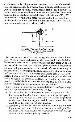
an old favorite is being attacked. So some, to whom the cathode

follower has seemed to be a valiant knight slaying all the electronic

bugs, take a fighting stand. When triodes aren’t “good enough” in

other circuits we turn to better tubes, such as pentodes. They havebeen used successfully as cathode followers, the circuit of Fig. 1224,

being typical. Doesn’t this arrangement enable low distortion to

be obtained into a low load value, since pentodes “like” workinginto low impedances better than triodes?

Fig. 1224. The cathode-follower circuit

of Fig. 1223, redrawn to show pentodetube operation.

It’s not as easy as that. Continuing with the example figures

used: With a triode, reduction of the plate load from 30,000 to

600 ohms—a ratio of 50:1—only reduced the gain from 20 to 1.2

because of the triode’s relatively low plate resistance. Because of

the very high plate resistance of a pentode, the corresponding re-

duction would be almost in the same ratio as the change in plateload resistance. Even if the pentode had a high gain to start with,loading it down with 600 ohms would reduce the gain as with thetriode, so again the effect of feedback in cleaning up waveformwould be negligible. In the end, the pentode does no better underthese conditions than the same tube used as a triode.

Now don’t start throwing out cathode followers. Let’s get things

really straight by recounting what they can do.

1. It is true that they reduce output source impedance. Their

limitation is that this feature must not be imposed upon by

assuming that we can go ahead and use a load impedancemuch lower than the regular load impedance for the tube

used. If we try that, we run into trouble.

2. Another good use for cathode followers is to obtain a very

high input impedance. This they also do very well, provided

the plate load (connected in the cathode) is kept high enoughto preserve the normal gain of the tube.

239

Now let’s look around to see how all this affects the circuits com-

monly used. Probably the most frequent everyday application of

the cathode follower is in the output of preamplifiers to provide a

low source impedance suitable for line-impedance connection be-

tween the preamplifier and the main amplifier. Before throwing

that poorly operating preamplifier out, check what the main

amplifier input impedance does to it. If it has a line-to-grid trans-

former, the cathode follower is undoubtedly being loaded downtoo much, and distortion occurs. If the main amplifier is arranged

for input direct to grid, the cathode follower will be quite happy,

and its low impedance will give the advantage of line impedance

coupling between amplifiers, i.e. freedom from loss of “highs” andfrom “static” pickup.

Summarizing the foregoing further, the right answer works out

this way: If the main amplifier uses transformer input, either for

phase splitting or to save gain or both, then the preamplifier out-

put should be properly matched down through a transformer,

whether plate or cathode coupled. On the other hand, if the input

end of the amplifier is all resistance-loaded, with nice high-value

resistors, the cathode follower direct is O.K. in the preamplifier

output.

So take another look at these circuits: you may rid yourself of

an unsuspected source of distortion.

240

chapter

13

high-power amplifiers

Feeding a number of speakers from a single amplifier has caused

the public-address man many a headache. It can also be quite

a problem to the hi-fi man who plans a distribution system for his

audio. It’s not always easy even when all the units have the same

impedance and require equal proportions of the total power,

though the problem is then theoretically simple. When the

problem includes units of different impedances requiring different

proportions of the power, it can become a real headache.

The constant-voltage system of distribution eases the situation

considerably, and generally does a much better job than the older

methods. Such systems have become very common in Europe andare fast gaining ground in America. They are usually designated

by the nominal voltage used. The American standard is a 70-volt

line; the European, a 1 00-volt line.

The constant-voltage system has one apparent disadvantage—

a

separate output transformer is required for each speaker. How-ever, this disadvantage is more apparent than real. True, when anamplifier is working only one speaker, located close to it, there is

no point in using more than one transformer for matching the out-

put to the speaker. Doing the matching in two steps adds to the

cost by one transformer, and also adds slightly to the audio losses.

But when the amplifier is feeding a number of speakers, matchingproblems may well make separate transformers worth while.

Voice-coil impedances range from 2 to about 16 ohms. (Some-

241

times values outside this range are met, but they are not common.)

Let us take 12 ohms for some examples because it makes cal-

culating easier. Suppose eight such speakers are connected, all to

receive the same power. The arrangements shown in Fig. 1301

give over-all impedances of 1.5, 6, 24 and 96 ohms, ft is probable

that even a multi-ratio output transformer will not provide most

of these matchings, so some other arrangement must be figured

ALL 12a SPtAKtBS

Fig. 1301. Four ways of connecting12-ohm speakers to receive equal power.

out, including one or more resistors as “dummies” to pad out the

values. The number of speakers in an actual installation may not

be so convenient for series-parallel connection as our example of

eight.

Suppose next that all speakers still have the same coil imped-

ance, but it is desired to feed them at different levels. Fig. 1302

shows two arrangements. Both give LSI four times the power re-

ceived by LS2 or LS3. These arrangements are fairly simple, but

the evolution of a suitable circuit for larger numbers becomes dif-

ficult.

The constant-voltage line simplifies all these problems, makes a

far more versatile system and is well worth the extra cost of a trans-

former for each speaker. There is another advantage. It is always

best to operate dynamic type speakers in parallel, otherwise elec-

trical damping is lost and peculiar effects due to interaction be-

tween speaker impedances are noticed. In constant-voltage opera-

tion, all units are always parallel-connected, even when the power

delivered to different units is varied. If numbers of speakers are

242

operated in parallel by direct connection, the resulting impedance

is so low that much of the output power is lost in connecting lines

unless very large cable is used. In the constant-voltage system, im-

pedances can be kept up to a reasonable figure.

A nominal line voltage is chosen, usually 70 or 100. This forms

the basis of all the calculations. This does not mean that there is

aliuaysdi signal of 70 or 100 volts, because it naturally fluctuates as

audio signals always do. The stated voltage represents a nominal

Fig. 1302. These hookups give four times as much power to LSI

as they do to LS2 or LS3.

maximum, output level. Perhaps the easiest way to get the idea is

to think in terms of a sine-wave signal, fully loading the amplifier.

The amplifier then can be regarded as providing a constant voltage

for all the speakers connected to the line, just as an electric line

does for all the appliances connected to it. The generator at the

power station has a certain maximum load capacity, and con-

sumers’ loads may be connected until that capacity is reached, the

power taken by each depending on its load impedance and the

line voltage. We are quite used to referring to electric lamps and

other appliances as “110-volt 40-watt,” but the same method of

rating speakers may seem strange at first.

Each speaker is fitted with a transformer to match its voice-coil

impedance up to an impedance which accepts the desired wattage

when the nominal voltage is applied. Some speakers may be fitted

with multi-ratio transformers so their power rating can be ad-

justed. This makes an installation very versatile and avoids the loss

of power caused when an individual volume control is used oneach speaker. You simply vary the number of watts accepted by

the speaker. Different voice-coil impedances are also taken care of

by the speaker-matching transformer.

Fig. 1303 illustrates an ideal calculation. LSI and LS2 each have

an impedance of 5,000 ohms, so they will accept 2 watts each at

100 volts. (Use Ohm’s law or the chart of Fig. 1304.) LS3 has a

voice-coil impedance of 2 ohms, and uses a transformer of ratio 70

243

to 1. From the chart of Fig. 1305, this gives an impedance of al-

most 10,000 ohms, which from the other chart rates at 1 watt for

100 volts. The total wattage load is 2 + 2 + 1 = 5. Using the chart

again, this corresponds to an impedance of 2,000 ohms (still for

100 volts). So an amplifier to supply just this load would need to

supply 5 watts matched into 2,000 ohms.

jor jgjjC5kT/2W V5Kji/2» IOKji/IW

Fig. 1303. A constant voltage line,

with the speakers receiving unequal

power. The amplifier unit would have

to supply 5 watts matched to 2000

ohms for this load (see text).

A large amplifier may be used to supply a load smaller than its

own output. For example, suppose a 60-watt amplifier is used to

feed the foregoing case requiring only 5 watts. The nominal volt-

age is used to calculate both LS and amplifier output impedances.

A 60-watt output for 100-volt operation should be matched into

170 ohms. The load actually connected is 2,000 ohms. Some ampli-

fiers working into a light load like this will be unstable. To pie-

vent this, a resistance load may be added to absorb the surplus

power. In the example suggested, a resistance load to absorb 50

watts would be adequate, and from the chart the value required

is 200 ohms. If the amplifier were to be operated continuously at

maximum output, this resistor should have a dissipation rating of

50 watts, but in practice a much smaller (10- or 20-watt) resistor

could be used.

Sometimes the reverse of the previous problem arises. The

nominal load connected exceeds the power output of the amplifier.

Here matters are adjusted by a different method. Suppose the load

is made up of a number of speakers rated at 2 and 5 watts for 100-

volt line, adding up to a total load of 80 watts. The load imped-

ance of 80 watts’ worth of speakers will be 125 ohms. The load for

a 20-watt amplifier, 100-volt working, would be 500 ohms. Apply-

ing a 125-ohm load to the otuput of an amplifier designed for 500

ohms would probably cut the output down to about 5 watts, and

as well likely cause distortion. So the output must be matched to

the actual speaker load of 125 ohms, which, according to the chart

of Fig. 1304, will give 20 watts at 50 volts, instead of the original

basis of calculation, 100 volts. This means the nominal 2-watt

speakers, of 5,000 ohms impedance, will get l/2 watt, and the nom-

inal 5-watt speakers, of 2,000 ohms impedance, will get 1 1/4 watts.

Note that this is a reduction of only 6 db, so quite a useful volume

244

will be available, although the amplifier is smaller than one

planned for 100 volts. Anyway, if the 4-to-l mismatch were used,

giving only 5 watts or so, there would be loss of another 6 db and

probably considerable distortion.

Use of the constant-voltage system does not necessarily meanspecial speaker transformers must be used, so a word about picking

suitable transformers from stock lines is needed. Makers of speaker

Fig. 1304. A constant-voltage chart showing the relationship of

impedance vs. voltage.

transformers mark them variously in turns or impedance ratio. In

the former case the chart of Fig. 1305 enables the correct turns

ratio to be found, but the actual turns on each winding must suit

the job too. A mike-to-line transformer for a ribbon microphone

may have the same ratio of turns as a speaker transformer, but

this does not mean that either would do the other’s job success-

fully. A good rule for checking the suitability of speaker trans-

formers with an ordinary ohmmeter is that the winding resistance

should be between 2% and 20% of the impedance for which it is

to be used. Less than 2% means its inductance will most likely be

245

inadequate, and 20% or more means the windings will absorb an

appreciable portion of the available audio power. If the resistance

of the voice-coil winding is too low to register on the ohmmeter

scale, the resistance of the high side should be compared with its

working impedance. Thus, for example, a winding intended to

work at 5,000 ohms should have a resistance that lies somewherebetween 1 00 and 1 ,000 ohms.

Where transformers are specified by impedance ratio—for ex-

ample, 7,000 ohms to 3.5 ohms—the maker has stated the best im-

pedance at which to work the transformer. Using these imped-

ances, it may be expected to be well over 90% efficient and have

a good response at low frequencies. But these are not the only im-

pedances at which the transformer can work. The important thing,

of course, is that the ratio of impedances hold true, so the same

transformer could be used for 4,000 to 2, 10,000 to 5 ohms, etc.

As stated in the previous paragraph, the losses and response mustbe kept within bounds. If impedances more than two or three

times the rated values are used, the transformer’s inductance mayprove inadequate. If it is used with impedances less than one-third

to one-half the rated values it will become quite inefficient.

A few years ago we built an amplifier with 50 watts output.

Using a special multi-ratio output transformer of personal design

provided matching for load impedances of 8, 12.5, 20, 32, 50, 80,

125 and 200 ohms. It can feed a few high-power units direct, using

appropriate matching, but more often it is used for 100-volt line

distribution, feeding various numbers of speakers. Up to 50 watts

nominal loading, the 200-ohm matching is used. If a greater load

has to be fed, a lower impedance matching is selected. The outfit

is extremely compact, and on various big sound reinforcement jobs

where it has been used, many engineers have been amazed that so

small an amplifier, with only 50 watts output, can provide suchlarge coverage. The secret lies in making the best use of the watts

available. This is just what correct use of the constant-voltage tech-

nique enables the public-address man to do.

It is only a matter of a little arithmetic to expand power dis-

tribution systems, once the basic principles are grasped. Whenother multiple connections are to be made, more complicatedproblems arise.

Hookup problems

Occasions frequently arise where the audio man has to feed two

246

or more independent sound systems from the same program

source. Electrical hookup between separate systems is often

fraught with difficulties. The most common solution is to run out

a separate microphone for each system to be tied in, resulting in

the veritable battery of microphones often seen when a celehrity

speaks on an important occasion. This method has serious disad-

vantages, the greatest of which is the variation of level, wheneverthe speaker moves or turns his head, on some of the systems whosemicrophones are not so well placed as others.

The best approach to the problem would be to use only one

high-quality microphone (with an extra one as a standby) to sup-

ply all the systems. This would simplify program pickup as well as

monitoring problems on each of the systems hooked together.

There would still be problems, but they need not be insurmount-

able once they are understood.

The chief problems may be listed under four headings:

1 . When two systems are coupled together, a severe line humoften develops in one or both that was not present in

either before the connection was made.

2. It may be difficult to provide the right impedance match

between the two systems without affecting the volume

level in one or both.

3. Where several systems are fed from a common source there

may be interaction between controls on the different sys-

tems. One operator altering his volume or tone-control

settings may affect the volume and quality of the signals

delivered to other parts of the hookup.

4. One or more systems in the hookup . . . recording units

for example . . . may not require the entire program; and

may adopt different methods of cutting in and out of the

network. Precautions must be taken to see that any such

circuit modifications in one part of the system do not inter-

fere with the rest of the hookup.

500-ohm bus system

By far the most versatile method is to set up a 500- or 600-ohm

balanced line that serves as a basic interconnecting bus. The best

arrangement is to have a microphone amplifier that will deliver

an output level of about 1 volt into a balanced 600-ohm line

(0 VU), but this is by no means essential. Any good amplifier with

the necessary microphone-control facilities can generally be made

247

to serve this purpose by padding the output to 500 ohms.

With this system not only can a program from a single source be

fed into a number of systems, but also various program sources

can be brought into the hookup by using separate local amplifiers

to feed into the 500-ohm bus at the desired points. Much of the

hum trouble can be eliminated by careful attention to impedance

and level matching. However, an important cause of hum that

cannot be taken care of in this way is that due to differences in

potential between the ground connections of the individual sys-

tems.

Ground potentials

In the interests of public safety, all power circuits are connected

to ground somewhere, and a ground connection also is provided

on some power-supply outlets as a safety precaution. The associa-

tion between the ground connections of the various supply circuits

in the building sets up small currents at the line frequency in the

grounded framework. These currents in turn set up slight poten-

tial differences, usually only a small fraction of a volt, but even

such a minute potential can create a serious hum if it gets into

any high-gain amplifier. This often happens when two systems are

coupled together, so the solution rests in careful selection of

ground-connection points.

While on this subject, it is well to mention that a good-quality

power amplifier should operate well with or without a groundconnection, and the effect of breaking or making this connection

should be almost inaudible—even with the volume turned to max-imum and the ear close to the loudspeaker. If an amplifier does

not satisfy these requirements, it is wiser to leave it out of anyhookup system and look for a better one. If no better amplifier is

available, then careful treatment may produce passable results, as

we will later explain.

Getting on the bus

Assume that we have a microphone amplifier delivering an out-

put of 1 volt into a 500-ohm balanced line, and we are going to

feed a number of sound systems from this line. Most amplifiers

designed for PA use are provided with separate microphone and

phono inputs. The microphone input is generally the best one to

match the 500-ohm line to, because it will have adequate reserve

248

of gain, whereas the phono input may not. Microphone inputs are

usually low-impedance, between 10 and 50 ohms in which some

are balanced to ground; some may be floating and some may have

one side connected to chassis.

Fig. 1306 shows the simplest method of connecting the line to a

balanced microphone input. For a single-ended input it may be

possible to unhook the ground connection inside the amplifier.

-r°4-30

4- IMPEDANCE

2/1-H

3/l-t

5/1- -

6/ 1-

-

t/\\ 310/1- =

TRANS TURN5ratio :

20/1- -

30/1

80/1—

P

Fig. 1305 . A chart for obtaining the line impedance fromthe turns ratio.

but this may give rise to trouble because the ground connection is

probably included to maintain stability in the amplifier. If this is

removed, and the input circuit is grounded only at some remote

point, hum trouble will probably appear.

Fig. 1307 shows one method of connection where one side of the

amplifier input is grounded. This may give trouble for two rea-

sons: The unbalanced line is likely to pick up hum or crosstalk

from telephone lines or other speech circuits that may run near it,

and the small potential difference between the two ground con-

nections may inject a line-frequency hum.

Fig. 1308 shows an alternative method of connection that avoids

strapping the two ground connections together as in Fig. 1307,

and also provides a balanced connecting line. One of these two

methods of connection should prove satisfactory. When going into

low-level low-impedance inputs, the resistor values should be ad-

justed so the resistance from both lines to ground is equal at the

distributing center. If this is checked by d.c.-resistance measure-

249

ment, all amplifier inputs and outputs should be disconnected, or

the winding resistance of their input and output transformers will

invalidate the result.

Most high-impedance phono or crystal-microphone inputs are

unbalanced. Fig. 1309 shows the simpler method of connectionhere corresponding to Fig. 1307 for low impedance, while Fig.

Fig. 1306. Method of connecting a

balanced-input amplifier to a balanced500-ohm line. Series resistors in the

padding network reduce loading andallow several amplifiers to be fed. from

one line.

1310 shows the method to adopt where a balanced line is necessary.

Line impedance

An important feature to realize about these circuits is that the

impedance of the connecting lines must be in the vicinity of 500

ohms. This is achieved in each of the circuits shown by inserting

padding resistors at the receiving end of the line. Two factors fea-

ture in the reason for this precaution: (a) transmission losses; (b)

pickup of hum or crosstalk.

Lines run at low impedance—that is, by putting the resistor net-

works at the output end of the line as in Figs. 1306, 1307 and

Fig. 1307. Method of feeding on un-balanced-input amplifier from a bal-

anced line. Potential differences be-

tween the two grounds may introduce

hum at the power frequency.

1308—introduce line loss due to the fact that the line-conductor

resistance may be an appreciable fraction of the operating imped-

ance. Such low-impedance circuits are also more susceptible to in-

ductive pickup from magnetic hum fields through which the line

may pass. The currents induced in the line will be of the same

magnitude whether the line is 500 ohms or low impedance, but

in the case of the 500-ohm line they will be attenuated by the pad-

ding network at the receiving end.

Lines run at high impedance—that is, by placing the padding

resistors of Figs. 1309 and 1310 at the opposite end of the line-

cause excessive loss of high frequencies due to line capacitance.

The line is also prone to pick up noise from electrostatic fields. Ofthe two extremes a low-impedance line is preferable because the

,HI VALUE

" S *UNBALANCED LINE

1

PADDING NETWORK !

oStrib center tear0

250

inductive components it picks up predominate at very low audio

frequencies, which may not get through the average PA ampli-

fier-speaker combination, while the static pickup in a high-imped-

ance line contains high-frequency components with a greater an-

noyance potential. Loss of high-frequency signal components in

the high-impedance line interferes with program quality.

Physically a balanced 500-ohm line is generally made up of a

twisted pair run inside flexible shielding. High-impedance lines

Fig. 1308. One method of reducinghum is by the insertion of an isolatingresistance between the two groundpoints. This arrangement also pro-

vides a balanced connecting line.

are usually single-conductor shielded wire, coaxial line or an un-

shielded twisted pair with one of the conductors grounded.

Besides providing good program quality with freedom from

spurious pickup, the correct padding network, properly placed,

will usually take care of problems 3 and 4 listed at the beginning.

The values of the padding network should be chosen so that what-

ever happens at the outlet end will not materially affect signal

voltages at the input end.

Ij^

L 1 L,270a

j

UNBALANCED LINE*j

PADDING RES

j

! UNBALANCED AMPL INPUT

DISTRIB CENTER

Fig. 1309. A simple method of feeding an unbalanced high-imped

-

ance input from a low-impedance unbalanced audio line.

For example, phone plugs and jacks are sometimes used as input

connections to an amplifier. When a plug of this type is inserted

into its jack, the line connected to the plug is shorted momentarily.

If the main 500-ohm line is connected to the plug, then insertion

or removal of the plug would momentarily short-circuit the whole

program. Inserting a padding network between the line and the

plug avoids this. In some tape recorders inserting the input plug

disconnects the playback head, so that if an operator wishes to

listen to a section of recording on his tape he has to remove the

251

input plug. Unless the foregoing precaution is observed this opera-

tion could involve interference with the program.

Another wise precaution is to see that all padding resistors are

soldered securely to the lines (once the values have been satisfac-

torily determined by experiment) and are suitably covered with

Fig. 1310. The method for connecting a balanced low-imped-ance line to a high-impedance single-ended amplifier input.If additional units are fed from the same line, the value ofthe shunt resistors in the padding network should be

increased.

insulating tape or otherwise protected against any possibility of

accidental short circuit or contact that might interfere with the

program in any way.

Improvising outputs

The foregoing assumes that a suitable microphone amplifier

with a balanced 500-ohm output is the signal source for the entire

network. If such an amplifier is not available, additional padding

will be necessary to match the output of the microphone amplifier

to the 500-ohm bus. If the amplifier has the usual low-impedance

Fig. 1311. Padding out a low-imped-ance output winding to feed a 500-

ohm line. The 270-ohm resistors

should be connected in series witheach end as shown (see text).

voice-coil output, a dummy load equal to the proper voice-coil im-

pedance should be connected across the output, after which re-

sistors of 270 ohms should be connected in series with each side of

the line as shown in Fig. 1311.

The voice-coil winding should not be connected to ground on

either side, or the line will not be balanced. If the amplifier re-

quires a ground connection to the voice-coil winding for satisfac-

tory operation, the dummy load resistor should be center-tapped

or made up of two equal resistors and the ground connection made

252

to the center tap as in Fig. 1312. If the secondary of the output

transformer is used for feedback purposes, one side will be con-

nected to the internal amplifier ground and the other side through

a suitable resistor to the appropriate feedback point. In this case

the modification of Fig. 1312 would cut the feedback in half. Torectify this, the feedback resistor also should be halved. The sim-

aDISCONNECT HERE;

Fig. 1312. The changes required whenone side of the voice-coil winding is

grounded.

plest procedure in this case, involving minimum alteration to the

amplifier (this is something that must always be borne in mindbecause the amplifier must be put back to normal after the hook-

up), is to disconnect the ground connection from one side of the

transformer secondary and connect it to the center tap of the dum-my-load resistor. Then shunt the feedback resistor with another

resistor of the same value. These changes are shown in Fig. 1313.

Most amplifiers can be treated in this way to supply the neces-

sary 500-ohm output, but you may find one that has high-imped-

AMPl OUT m-—

m

*<V0ICE COIL OUMMT LOAD ^FEED-BACK RES

SHUNT.RES

MAKE THIS CONN

—DISCONNECT HERE

TFig. 1313. Circuit modifications requiredwhen the output-transformer secondaryis part of the feedback network (see text).

ance output above 500 ohms. We have frequently used an ampli-

fier with 2,000-ohm output (intended for constant-voltage-line

work) for this purpose. The procedure is similar in this case, but

the series resistors will have to be much higher than the line im-

pedance. This type of network is shown in Fig. 1314.

253

Multiple signal sources

Where programs are to be taken from more than one source in

the system, it will be advantageous to feed the 500-ohm bus from

a local microphone amplifier or phone preamplifier at each point

of origin. If the amplifier is one specially designed to feed a 500-

t Fig. 1314. Padding a network forC*' matching a high-impedance output[270 MO* BUS transformer to feed a balanced 500-

| ^ohm line. In this case, the series re-

sistors must have a much greater

value than the line impedance.

ohm balanced line, additional precautions are necessary to see that

its operation will not interfere with programs originating from

other amplifiers. The plate resistance of the output stage is usually

much lower than its load resistance, which means that, even

though it is connected to a 500-ohm output circuit, when the am-

plifier is warmed up, a signal from another source will “see” this

output circuit as 500 ohms shunted by the plate resistance, or

much less than 500 ohms. Now suppose the amplifier is switched

SHIELDED III LINE TRANS

CONN TO SYSTEM GND

B- BUS IN AMPL

Fig. 1315. An isolation transformer may be needed to

reduce hum when feeding an a.c.-d.c. amplifier with a

floating B-minus return from an audio line.

off. The shunting effect of the plate resistance disappears and the

other amplifier will be feeding into a circuit that has now risen to

its true 500 ohms. Thus, switching the first amplifier on and off,

although it may not be carrying any program, will affect the out-

put from a second amplifier, changing its volume level by from 10

to 20 db.

From this viewpoint, amplifiers with padding networks may be

better than those specifically designed for 500-ohm output. For

the correctly designed amplifier, the best plan is to insert a resistor

of 150 ohms in series with each side of the line at the output to

limit the reduction in shunt impedance when the amplifier is on,

254

as viewed from another amplifier feeding the 500-ohm bus. This

will take care of impedance matching, but may still leave a possible

change of level of about 6 db should the amplifier be switched onand off while the program is coming from the other source. A wise

precaution is to establish a recognized rule that the amplifier must

LINE TO SPKR TRANS (CONNECTED AS STEP-DOWN)

B-BUS IN AMPL

Fig. 1316. Another method of connecting an a.c.-d.c. am-plifier to a 500-ohm line. The potentiometer across the

input terminals is for balancing out line hum.

be kept running throughout the whole program whenever any

part of the system is being used. This rule may not be necessary

with amplifiers padded out from lower or higher impedance to

500 ohms.

i:i pwrline isolatino trans

+ III PWR-UNE ISOLATING TRANS

Fig. 1317. Isolating the a.c.-d.c. ampli-

fier from the power line. A 1:1 powertransformer for a.c. operation is shownin (a). The same transformer con-

nected as a dual choke for operation

from d.c. power lines is shown in (b).

Isolating grounds

The padding arrangements shown in Figs. 1306 through 1310,

usually prove perfectly adequate with good amplifiers. Sometimes,

however, an amplifier must be pressed into service which does not

meet the conditions specified earlier of satisfactory operation with

or without a ground connection. Many amplifiers designed for

universal operation come in this category. Complete isolation

255

must be provided between the system ground and the chassis (or

ground bus) of this particular amplifier.

Several methods of attack can be tried, and the choice will be

controlled by the equipment available. If a shielded line-to-line

transformer is available, the method shown in Fig. 1315 shouldbe satisfactory. If only a line-to-speaker matching transformer or

some such component is available, the circuit of Fig. 1316 can beused. The potentiometer may be almost any value, as long as it is

higher than the other components in the circuit. It is used to bal-

ance out hum pickup.

An alternative approach is to use an isolating transformer be-

tween the power line and the amplifier in question. An exampleof this is shown in Fig. 1317-a. An isolating transformer also can

be used as shown in Fig. 1317-b when the supply is d.c. with the

wrong side grounded.

Remote microphone control

This application in public-address and sound-reinforcement

work has obvious advantages, and once you try it you’ll find it in-

dispensable. The control panel can be moved to any convenient

point where the operator can hear what the audience hears and

and can watch the stage for cues. The simplest method of remote

control is electronic mixing, using d.c. bias on the control or sup-

pressor grids of the individual microphone-input stages. The chief

advantages of this method are that low-level audio signals go direct

to the amplifier inputs instead of first passing through noisy

switching circuits, and the control lines carry only hum-free d.c.

The d.c. bias supply can be a dropping resistor in the commonnegative return, or a well filtered d.c. heater supply for the first

stages can be used. Either way there must be sufficient decoupling

and filtering to keep hum or noise off the grid used for gain con-

trol. Simple resistor-capacitor filters are sufficient.

On jobs where two or more microphones are required there will

be less danger of acoustic feedback if only one microphone is alive

at any time, or at least if only those microphones actually needed

at the moment are alive. This is no problem with direct micro-

phone switching, but a remote-control switching circuit is not easy

to design. If bias voltage is switched, loud clicks or plops comefrom the system. One alternative is to change the bias quickly with

fader type controls, but this can cause peculiar effects until a great

deal of skill is acquired; and with nice fat decoupling capacitors

256

in the circuit, there can be a disconcerting delay in the micro-

phone changeover action.

The problem is to provide the quickest possible change of bias

without any audible effect. The solution is an automatic switching

circuit (Fig. 1318)

.

Various arrangements were tried for smoothing out the switch-

ing clicks, from a single R-C combination to a multisection low-

Fig. 1318. The circuit of the basic

bias-control unit for one microphone.The three-section filter eliminates au-dible switching transients without any

noticeable delay.

pass filter. A single resistor-capacitor section produced a loud click

unless the values were made so large that the time delay became

unbearably long. With multisection filters the click was trans-

formed into a plop; the filters changed the proportions of the com-

ponent frequencies in the switching voltage transient.

High-speed switching means that some disturbance (in the form

of a simple step transient) is bound to get into the amplifier. The

problem is to make this transient inaudible, while still attaining

satisfactory operating speed. To do this, all the component fre-

quencies in the step must be inaudible. We dug out an old copy

of Fletcher-Munson loudness contours, from which we found that

the slope of the curves at the low-frequency end is approximately

18 db per octave near the threshold of audibility. The answer was

to use three R-C stages, each with a slope of 6 db per octave, to

produce an inverse modification of the step response. This should

give the highest possible speed of action without producing any

audible effect. It worked! When this system is in use, there is not

the slightest indication that at one instant a certain mike is dead

and a second later it is alive.

Two systems were modified to incorporate this method of

switching. The first was simply a twin version of Fig. 1318 for

switching two microphone circuits. The second is far more versa-

tile and is shown in block form in Fig. 1319. There are three re-

mote-control microphone inputs with universal input transform-

ers so that microphones of any impedance can be used. After mix-

ing, the frequency spectrum is divided into three channels, with

individual low- medium- and high-frequency amplifiers. Two of

the channels have remote gain control (operating the middle

channel at fixed gain eliminates an extra control).

257

6J7’s are used in the input and tone-control stages. Tubes were

scarce in England when the original amplifier was built, and the

6J7 and the Z63 (a British type) can be used interchangeably.

With the control bias applied to grid 1,12 volts provides completecutoff. This is much less than would be needed with remote-cut-

off tubes, and no microphone has large enough output to produceappreciable distortion due to the curvature of the tube characteris-

tic even in the second stages.

1ST STAGES 2ND STAGES

REMOTE BIAS OPERATED GAIN CONTROL UNIT WITH MASTER FADER SWITCH

Fig. 1319. Block diagram of the deluxeremote-control amplifier described in thetext. One or more microphone inputsmay be selected, mixed and divided intolow-, medium- and high-frequency ampli-fier channels with independent gain

Grid 1 control was chosen in preference to suppressor control

because the earlier KTZ63, for which the Z63 is now a replace-

ment, was a tetrode. Use care in selecting tubes to find suitable

nonmicrophonic samples. Special low-noise pentodes such as the

1620, 5879 and British EF37A might be better for this application,

but this does not invalidate the method. Fig. 1320 is the complete

amplifier circuit.

The control-panel circuit is shown in Fig. 1321, and the remote-

control connection is through an octal plug and socket on a

7-wire cable.

There are two switches with each microphone gain control. The

lower one (SI, S2 or S3 in Fig. 1321) is a simple on-off toggle

switch: when it is off, that mike circuit is definitely off. When it

is on, the mike is controlled by the remaining switches and con-

trols. The additional switch above each gain control (S4, S5 or

S6) has three positions, marked a, on, b; in the center (on) posi-

tion, the mike circuit is on, subject to control only by gain controls

258

Rl, R2, or R3. But in either side position A or b it is further sub-

ject to control by the tone-control switch S7.

Two pairs of tone-compensation controls—one pair shown a;

R4 and R5, and the other pair shown as R6 and R7—are providedfor low-and high-frequency gain. (The mid-frequency gain is pre

Fig. 1320. Schematic diagram of the deluxe remote-controlled amplifier de-

scribed in Fig. 1319.

set in the amplifier.) Between these pairs is a two-way switch S7

whose positions have been marked A and b. When this switch is in

the a position R4 and R5 control tone, while in b position R6 and

R7 control tone. Besides selecting tone-control settings, this switch

will also select mike circuits set to position A or b on the indi-

vidual mike-circuit switches.

This layout may seem complicated, but a little thought will

show that it provides extremely versatile control. Suppose two in-

dividuals are talking alternately into two different mikes. Using

S4 and S5, one mike can be set to a position and the other to b, and

the master tone-control switch S7 can be used to switch from one

to the other as each speaks in turn. Tone control group a can be

set to give the most pleasing result with mike and voice A, inde-

pendent of the b position setting. S7 changes the tone setting auto-

matically every time the mikes are switched. If desired, a third

mike can cut in on either a or b position by having its three-way

circuit switch S6 in the on position and just bringing it in with its

on-off switch S3. It is best to keep any circuit not in use with its

on-off switch on off and its selector switch in the middle on posi-

tion. Then it can be cut into the circuit instantly, simply by throw-ing the on-off switch. The high- and low-frequency tone controls

can be used to create special effects such as artificial distance bvaccenting or attenuating extreme frequencies.

One feature of the panel’s versatility is that a new tone-control

setup can be prepared while one or two mike circuits are beingused. At the right moment the changeover between the tone con-

trols is made with a flick of the a-b switch S7. If for any reason the

new arrangement would be better on b circuit, and the presentarrangement is already on it, then the present setup can be trans-

ferred to A circuit first. Set the live mike-selector switches to the

middle on position set both tone controls in the same position andchange over from b to A with S7. Then switch the live mike select-

ors to a. Now preparation can proceed on the b circuit. This doesnot interfere with the program. A little thought is needed to

master the principle of operation, but once understood its extremeversatility is ample reward.

Two more points should be made clear before concluding. Thevalues used for the switching-filter circuits, three 150,000-ohm re-

sistors and three 0.1 -pf capacitors, proved adequate for practically

all jobs. If more than usual gain is required, due to using a low-

sensitivity microphone at long range, switching clicks may comethrough, particularly when switching off. One method of prevent-

ing this without modifying the circuit, is to turn the gain control

down first; then switch off and then reset the gain control to the

desired level ready for the next switching on. If the operator finds

this difficult, further controls could be added to reduce the gain

by a fixed amount in the off position (just enough to render the

microphone insensitive), instead of cutting the tube off complete-

ly. Less switching voltage will be needed with this method, but the

first method has been found satisfactory for the comparatively few

260

occasions where these particular clicks are eltectively audible.

Some readers may feel that 6J7’s will not give much range of

control, but will act like on-off switches. Try it. You will find that

any tube can be used as a variable-mu tube, provided the signal

level is small enough so the tube curvature does not cause distor-

tion. The range of gain variation is as great as can be obtainedwith a remote-cutoff tube.

Fie;. 1321. Schematic diagram of the remote control unit for use with the amplifier

of Fig. 1320.

The story of an amplifier

We shall now complete the cycle of discussion on high power

amplifiers. This section deals with an amplifier which has been

designed to act as a general-purpose public-address or sound

reinforcement unit. This is not an amplifier for the home, at

least not for our idea of a home. It was designed for use in a

sound-distribution network, feeding from 5 to 50 loudspeakers in

parallel. The particular merit of the design is its flexibility.

For distribution work in which a number of loudspeakers are

to be driven from a common audio line we are in rather the same

position as the power engineer who provides 60-cycle supply at a

number of outlets to drive the radio and the lamps, the vacuumcleaner and the electric heater. He provides us with a fixed volt-

age from a low-impedance source, so that the level at one outlet

does not depend on the load at another. The nominal level of the

60-cycle supply is 1 17 volts r.m.s. In distributing speech and music

to a number of outlets it is very convenient to follow this example,

but to use 50 volts r.m.s. as the nominal level. Loads of down to

50 ohms then can be connected to a 50-watt supply, and loads

down to 5 ohms to a 500-watt supply. If 10-watt speakers are used,

each is bridged across the line, with a transformer giving a pri-

mary impedance of 250 ohms.

The power supply engineer provides a low-impedance source,

then monitors the output so that the voltage does not vary morethan about 5% as the load is changed. We shall use negative

feedback to keep the audio level from varying more than about

20% as the load changes from one loudspeaker to the maximumsystem load.

Recently, we had to design a number of such systems of differ-

ent sizes. For practical reasons, we decided to design one basic

amplifier which could be used as a standard “brick,” in building

any size system. The standard unit which best fitted into the

scheme turned out to be a 100-watt amplifier, using four tubes in

the output stage. When operated with only two tubes it is a

50-watt amplifier, the power consumption being halved. Whenmore power is needed, several amplifiers can be connected in

parallel without any more precaution than the obvious check of

keeping the polarities the same. So far only five have been runin parallel, but there will be very few jobs for which more than500 watts of audio is needed.

This sort of installation is ideal for the ordinary operator.

With 500 watts of amplifier power he either can use it all at the

one big show, such as the county fair, or he can put in 200 watts

for one job, 100 watts for another, 50 watts in some small hall,

and still hold one unit in reserve. The equipment load factor canbe kept high, and he never has to use a big amplifier for a small

job where tube wear would eat away his profit.

The circuit

The amplifier circuit is a very simple one, consisting merely of

a seesaw phase splitter driving a class-B push-pull output stage.

In consequence, the grid input voltage is high, by the usual stand-

ards of power amplifiers (we need 15 volts to drive the amplifiers

to full power). This is only a few milliwatts, however, and is eas-

ily obtained from a normal three-stage microphone amplifier.

The voltage deliberately was made high so that the long connec-tions used in paralleling amplifiers would not pick up serious

262

amounts of hum and noise. Class-B operation hasn’t been too

well accepted because of its so-called resultant notch effect. This

is the small step at the crossover point where both sides of the

push-pull circuit seem to be cut off. With a bad transformer all

sorts of curious effects can occur in the gap, and if the transformer

is included in the feedback path, trouble is in store for the de-

signer. A good transformer, which must be symmetrical, seems

to prevent all this sort of trouble, and in this amplifier, at any rate,

the waveform looks pretty good until the level is high enough for

the peaks to start limiting. The notch effect, it is true, can be

caused by wrong bias; but so long as the values given by the tube

manufacturer are used, there is no trouble. Anyone who is sus-

picious about this might ponder on the number of AM broadcast

transmitters which use high-power class-B modulators. They dothis in Europe, too, where state-controlled broadcasting means that

low distortion is demanded with all the vigor that any taxpayer

puts behind what he considers his rights.

The output tube, which is the key to the amplifier design, is a

European type, the Mullard EL34. There just does not appear

to be any other tube which will do all that this excellent tube

will. It is a 6.3-volt indirectly heated tube, on an octal base, with

a transconductance of 10,000 phmos and can be run in class Bwith 0.5 megohm in the grid circuit. The full details are listed

separately1. Four of these tubes give a rated power output of 116

watts at 425 volts plate supply, and they can be driven by a single

1 2AT7. Every other tube seems to need a low-impedance driver

stage or an extravagantly high plate voltage.

What sort of a performance will this amplifier give? Measured

at 10 volts output into a 25-ohm load, the frequency response is

flat within ±1 db from 20 to over 10,000 cycles. At 100 watts the

distortion is less than 2% at frequencies between 300 and 1,000

cycles. It is not much more even at 75 cycles, but this is not

important, because we do not expect high levels at extremefrequencies.

l Mullard EL34 tube: Heater: 6.3 volts, 1.5 amps. a.c. or d.c. Class B operation, 2

tubes: Common screen resistor 800 ohms

Bias -42 v -42 vGrid drive 0 29.5 vSupply voltage 425 v 425 vOptimum load 4,400 Q 4,400 QIp 2 X 20 ma 2 X 106 ma

I,, 2 x 2.4 ma 2 x 28 maPower 0 58 watts

Distortion - 4.5%

263

Negative feedback keeps the output impedance low, so that

when the load is disconnected the output line voltage rises less

than 20%, hardly noticeable by a listener.

The circuit diagram is shown in Fig. 1322. The input tube, a

12AT7 double triode, operates as a seesaw type phase splitter.

The first triode is a normal amplifier with 47,000-ohm plate load.

Cathode bias is provided by a 2,000-ohm cathode resistor to-

gether with the 2,200-ohm feedback resistor, making 1,047 ohms.

This tube is used to drive the lower half of the push-pull stage.

The second triode is a unity gain amplifier with a large amountof feedback from plate to grid, which gets its input through

the first 470,000-ohm resistor. That, at least, is one way of look-

ing at it. Another way of thinking of the circuit is that the grid

drive of the second tube is the difference in the plate swings of

the two triodes, so that the center point of the two 470,000-ohm

resistors acts as the fulcrum of a seesaw. An exact balance of the

plate swings is obtained by reducing the left-hand 470,000-ohmresistor slightly. If you want to balance the stage closely, you can

try something of the order of 5 megohms in parallel with this

resistor or some tens of kilohms in series with the right-hand

resistor. The second triode drives the upper half of the push-pull

stage. The plate-supply voltage, about 250, for the twin triode is

derived from the main high-voltage supply of 425-475 by a poten-

tial divider and decoupling capacitor.

In the power stage all cathodes are grounded. Plate stoppers of

22 to 25 ohms, mounted close to each tube, kill any parasitic oscil-

lations which may otherwise be produced in the wiring. Each

push-pull pair has its own 800-ohm common screen resistor, which

is not decoupled. The screen voltage comes straight from the high-

voltage supply. Feedback is taken from the special winding on the

output transformer. With 42 volts bias on the output stage, a drive

of 29.5 volts r.m.s. is needed to give full output.

The output transformer

The design of the output transformer is the first and most im-

portant stage in the detailed design of the amplifier, once the

framework of the amplifier is fixed. In designing this transformer

for class B it is imperative to keep the leakage inductances low and

the balance between the two sides good. Balanced direct-current

polarization cannot be assumed, because we do not want to runinto instability if a tube fails. We can make the assumption that

264

we do not want high levels at low frequencies, and in designing

the transformer we have allowed the rolloff at low frequencies to

begin at 1 25 cycles, so that the plate load is almost purely resistive

down to 300 cycles, while the response is 6 db down at 60 cycles

In these circumstances the high-frequency response of the trans

former alone is good up to beyond 30 kc. The inductance is easil)

calculated. The optimum plate-to-plate load for two tubes is 4,00C

1322. The amplifier schematic. Feedback is obtained from a specu

output winding.

ohms, so that for four tubes it will be 2,000 ohms. The inductance

is 2,000 x 2 tr X 125=2.54 henries. With the core size shown in Fig.

1323, and an air gap of .040 inch, ordinary 14-mil silicon steel lam-

inations, we need 1,200 turns to give an inductance of 2.5 h. The

exact core size is not critical, of course, and any core of about the

same size may be used. Fig. 1323-a is a rough drawing of the core.

The plate windings are put on as four separate windings of 300

turns each, two in each section of a twin former. They are cross-

connected as shown in Fig. 1323-b. A layer of insulation, rated at

2,000 volts, is then applied. This can be supplemented with an or

dinary split screen of copper foil.

Over the plate windings three additional windings are added on

each half of the former. These are output, feedback and output in

that order. No. 18 AWG wire is used for the output windings,

while 30 AWG is used for the feedback winding. Each of these six

coils contain 65 turns. A series-parallel connection of the output

windings and series-feedback windings provide very close and bal-

anced coupling between the output circuit and the feedback wind-

ing. The wire turns and size appear in Fig. 1323-c.

Although this sort of amplifier is usually considered to be a two-

stage circuit, which must be stable at low frequencies, it must not

be forgotten that the signal in one half of the push-pull stage

passes through three stages. Adequate low-frequency stability is

obtained by choosing the coupling capacitors so that the response

is flat to well below the 125 cycles used in the output transformer

design. We have used 0.1 (if, which with the 100,000-ohm grid re-

sistors gives a characteristic frequency below 1 6 cycles per second.

This value of capacitance can be reduced to .05 (if without danger,

and could probably be reduced even more.

High-frequency problems

At the high-frequency end the design presented a lot of difficul-

ties, mainly because of the need for flexibility. An amplifier to work

into a normal load is quite straightforward; but if you want to be

able to remove the load or to attach a long capacitive cable with

no termination, the problems of design become much more com-

plicated. Separate responses must be plotted for each possible load

condition, and any circuit change must be checked in at least three

different plots. To add to the difficulty a really good safety margin

seemed to be desirable to meet the special conditions of parallel

operation. Two shunt R-C circuits, one in each stage, and dupli-

cated because of the push-pull operation, were found to give satis-

factory results. Across each half of the transformer primary a .02-(if

capacitor (1,000-volt d.c. working paper tubular) is connected to

prevent the load on the output side affecting the high-frequency

response. The phase shift produced by this capacitance is brought

back to zero in the dangerous region above 25 kc by connecting

400-ohm resistors in series with each capacitor.

An additional pair of high-frequency response control circuits

across the interstage circuits of the amplifier, consisting each of a

4,700-ohm resistor in series with .002 (if, was found to be necessary.

It would probably be sufficient to combine these into a single

10,000-ohm resistor and .001 (if, leaving out the ground point at

the center.

One disadvantage of the stabilizing system used must be noted.

At high frequencies all the power can pass into the two 400-ohm

resistors across the transformer primary. Any attempt to measure

266

the frequency response at full power will lead to a burn-out here,

unless you use unreasonably large resistors. We have used 5-watt

wire wound resistors, which do not even get warm under normal

working conditions. The only other resistors with any power in

them are the 800-ohm screen resistors, which should be 2-watt

types.

TURNS SIZE NO. TURNS SIZE NO.65 18 65 1 8

65 30 65 30

65 18 65 18

300 24 300 24

300 24 300 24

Fig. 1323. The data required for the de-

sign of the output transformer. Thecore specifications are shown in (a);

the electrical connections in (b); the

wire turns and size are listed in thetabulation box (c).

The physical layout can follow the circuit diagram. The only

precautions are to keep the stages separate and to keep the plate

stopper resistors in the output stage near the tubes. Do not forget

that the output line must carry 2 amperes.

Some important details

The power supply unit is required to provide 6.3 amp at 6.3

267

volts for the heaters, a plate supply of about 550 ma at full load,

dropping to about 100 ma at no input, with a smoothed voltage

of 425 at full load. In addition a smoothed grid supply of 42 volts

is needed. For the grid supply a germanium, copper oxide or sel-

enium rectifier may be used, and it is a good idea to take this andthe heater supply from one transformer. The grid-bias voltage can

be used to operate a relay in the high-voltage supply transformer

primary, so that you cannot get plate voltage without bias. Moretrouble, true, but so is paying for new tubes if the bias supply fails.

The bias must be adjusted to 42 volts with a resistor in the bias-

rectifier circuit. The high voltage is supplied by a 550-0-550-voltwinding and a pair of 5Z3 rectifiers. It is a good idea to make it

three 5Z3’s to keep the system working through a failure. A chokeinput filter, using a single 10-pf capacitor, provides sufficient

smoothing, and the regulation is such that the voltage at no loadrises to 475.

An additional continuity of service precaution is the connectionof a second 12AT7 in parallel with the one shown.When used as a 100-watt amplifier all tubes should be in place,

and the load impedance should be 25 ohms. It is, of course, quitein order to work with higher load impedances, but you will notget 100 watts, but only (50)

2/R watts, where R is the load imped-ance. If you need only 50 watts, pull out two of the EL34 tubesand one of the rectifiers, if you are using three. That is all. If youneed 200 watts, connect two amplifiers in parallel, after checkingthat they are set to have the same gain. The load impedance maythen be 12.5 ohms; and so on for higher powers.

268

chapter

14

test equipment design

Y ou will have read dozens of articles on new designs of high-

fidelity amplifiers: how often has the designer told you where

you can get a correspondingly high-fidelity input? If you

have 0.2 volt of input, you get 10 watts of true and faithful copy;

but copy of what? The output from a receiver of unknown per-

formance or pickup which seems to sound quite good? In the

ground-ray region, of course, there’s WWV. Elsewhere, a signal

generator must be used, and the average commercial unit is not

good enough.

Single-frequency generator

Faced with this problem, our solution was to build a special

signal generator. For our purposes, 0.5% distortion up to 50%modulation was good enough. Mr. Sampson of G-E has described a

similar but more elaborate circuit, which has 0.1% distortion at

100% modulation 1. Here, however, we shall describe our own

circuit with emphasis on feedback circuit design because it con-

tains all the basic elements to be considered.

The performance can be improved by elaborating the modula-

tor and detector but these do not involve the feedback loop. Thesignal generator is a single-frequency unit. The commercial design

by Sampson requires six adjustments when changing frequency,

i Electronics, April, 1949; Proc. Nat. Elec. Conf., 1948.

269

but for receiver testing it is always possible to tune the receiver to

the generator.

To simplify arithmetic, we shall not follow our own design ex-

actly, but will use a design carrier of 800 kc. Any type of modula-

tion may be used, so it is quite easy to run comparative tests on the

signal generator and receiver, using a microphone or tape record-

ing as source. A good audio oscillator is used for normal distortion

measurements.

Fig. 1401. Block diagram of the sin-

gle-frequency generator showing feed-

back components and loop. Except for

the detector in the feedback path andthe modulator within the forwardpath, this diagram could easily repre-

sent a feedback amplifier.

The block schematic is shown in Fig. 1401. It looks exactly like

a feedback amplifier, except that inside the forward path there is

a modulator, and in the feedback path there is a detector. Ideally,

just as in ordinary audio feedback, the performance depends only

on the feedback path, so that instead of needing to design a good

modulator, all we must do is produce a good detector.

In practice, just as we make our audio amplifiers as good as pos-

sible before we apply feedback, here we try to get a good modula-

tor because we cannot apply unlimited feedback. The problem is

to decide what we mean by amplitude and phase characteristics

when one part of the circuit works at audio frequencies and an-

other at 800 kc. First, consider the component parts of the system

which take the place of the individual stages of an ordinary ampli-

fier.

The oscillator circuit

The master oscillator circuit (Fig. 1402) is the highly stable

Clapp-Gouriet circuit. It was incorporated because we wanted to

see whether it was as good as reported. If a new oscillator appears

while you are building a signal generator, by all means try it! In

case you have forgotten about the Clapp-Gouriet circuit, we have

shown the bare bones of this circuit together with the Colpitts cir-

cuit in Figs. 1403-a and b. The conversion from one circuit to the

other is made by making the tank circuit capacitors of the Colpitts

very large, and the necessary small inductance to correspond is ob-

tained by series-tuning a normal-value inductance. The oscillation

270

frequency is just above the series-resonance frequency of the L-G

branch. The main disadvantage of this circuit in some applications

is the rather low output, but we need only about 1 volt for the

modulator grid.

The modulator

The modulator uses a 6AS6 tube. This is a rather uncommonapplication of the tube, but since it has a relatively high sup-

Fig. 1402. Circuit diagram of the master oscil-

lator used in the generator.

pressor mutual conductance, it will work in phantastron and other

similar circuits. In the 6AS6, 5 volts on the suppressor will cut off

the plate current. The exact figure depends on screen and plate

voltages. It makes a convenient modulator for this circuit because

the oscillator and audio inputs can be completely isolated by

applying them to separate grids. The circuit, shown in Fig. 1404,

provides cathode degeneration at audio frequencies: the 3,000-

ohm resistor is decoupled only to radio frequencies. The result is

Fig. 1403. Two basic oscillator cir-

cuits. In (a) is shown a typical Col-

pitts oscillator; in (b), the Clapp-

Gouriet oscillator. The latter cir-

cuit’s main disadvantage is low out-

put for certain applications.

that the modulator gives fairly low distortion up to about 50%modulation.

The output is taken via a cathode follower, so that the load does

not react on the circuit. The external load is tapped down on the

cathode-follower resistor, because we require only small outputs

and can use the decoupling produced by this resistive attenuator.

An external attenuator was used to control the level, but a tapping

slider on the 75-ohm resistor could be used. We can neglect the

frequency response of the cathode follower, fortunately, so that

we need not put in the actual circuit at this point.

271

Detector

The key to the feedback loop is the detector. A germaniumdiode, together with a filter circuit to eliminate the radio-fre-

quency components, provides audio voltages which can be con-

nected back into the audio amplifier. The circuit of this is shownin Fig. 1405. It would be a considerable improvement to add extra

carrier at this point to keep the effective depth of modulation very

low. The Sampson circuit does this but, unless you expect to bewmrking in the region below 1 % with your receivers, it is notworth going to the extra complication involved.

These bare bones must now be assembled into a complete cir-

cuit with its feedback loop closed. As we saw in Chapter 5 (designof an amplifier for 1.6 me), the r.f. stages operate right down to

zero-modulation frequency. Therefore, regarding low-frequencyaudio response, only one R-C circuit has any effect, and we cannotpossibly have low-frequency instability. All our attention is con-centrated on the problems that are presented by the high-fre-

quency audio response.

Circuit problems

Three circuits affect circuit behavior for high modulation fre-

quencies:

1. The plate circuit of the audio amplifier.

2. The plate circuit of the modulator.

3. The smoothing circuits in the detector.

Let us consider them separately, and put in numbers which look

reasonable. Should the results be unsatisfactory, we must make the

changes suggested by the shape of the curves. We are trying to

take the reader right along with us in working out the design.

Most of the interest lies in the spots where you go wrong!

The audio amplifier is quite conventional and its main purpose

is to provide a convenient means of connecting the feedback into

the circuit without requiring the use of a very large feedback

voltage.

The audio amplifier has a plate resistor of 100,000 ohms and a

total capacitance, including wiring, which should not exceed 20

ppf. The characteristic frequency is found by

1

272

1

CR 20 X 10- 12 X 10» 10-7 X 20= 500,000

Since « = 2-rrf = 500,000, then:

We can afford to put in a stabilizing circuit here, and a con-

venient design frequency is 8 kc. The capacitance is therefore 200

(t|if. If 20 u,[_if gives a frequency of 80 kc, then 8 kc will require

(since capacitance is inversely proportional to frequency) a figure

of 200 [igf. The point at which we flatten out the characteristics

settles the amount of phase shift we shall have, and we shall guess

the value of resistor to be used as 27,000 ohms. This makes the re-

sponse of the audio stage flatten out about 14 db down and moves

the final cutoff up to 400 kc. These values are the sort of values

we have been using in a lot of audio circuits, so this guess has

pretty strong inspiration.

For the plate circuit of the 6AS6 we can start from several dif-

ferent assumptions. To get stable tuning without the tube capaci-

tance having too much effect, the capacitance must be at least, say,

100 jx^f. The corresponding inductance, for a frequency of 800 kc,

is 400 ph, as shown in the following calculations:

2ir\/LC(115)

x/LC “2-7rf0

“ 6.28 x 800,000

VLx ioo x <o- =50^5

1

xl0.

273

Squaring, we get

uL ... 27rfL = 6.28 X 8 X 10* X 4 X 10~ 4 = 6.28 X 320

coL = 2,000 ohms

The plate impedance is 2,000 X Q ohms: Q is the figure of

merit of the plate-circuit inductance. The coil itself will give us

a Q value in the order of 100, but the tube characteristics suggest

that Q = 10, giving 20,000 ohms plate load, would be more suit-

able.

Let us look at it another way. You may remember that the band-

width associated with a given resistance and capacitance is un-

altered by moving from audio to bandpass problems. Since we are

to work with audio frequencies up to about 8 kc, the bandpass

bandwidth must be about 16 kc. Taking 20,000 ohms as the de-

sired resistance value, we have:

27rfCR = 1 (116)

2?rfR 6.28 X 1.6 X 104 X 2 X 104—

20 x 108

= 500 ufif

The use of 100 ppf, giving five times the bandwidth or 80 kc,

would mean that the envelope response was 3 db down at 40-kc

modulation frequency, and that the gain was only about 40 dbdown at audio frequencies. Too much audio would then comestraight through to the output. Let us switch designs to the 500-

ppf, 80-ph basis, and make sure that we get a Q of 50. (This induct-

ance value can be computed using equation 115 with the value for

C = 500 pgf, and f = 800 kc). An ordinary slug type, dust-corecoil will do the job.

In designing the detector circuit we have another problem. Wewant to keep the radio frequency out of the feedback loop, but yet

not produce too much phase shift at audio frequencies. The de-

tector network, of course, is an audio network; it is only in the

modulator that we have the bandpass type of circuit. To find whatwe need we must construct the amplitude and phase response

274

characteristics for the portions of the circuit already designed.

Those are shown in Fig. 1406.

If we assume that we want to put on 20 db of feedback, we can

take a 7-db margin and make sure that the phase shift is less than180° at 45 kc. Looking up low-pass filters in reference tables wesee that a full section of constant-K low-pass filter has a phase shift

of 180° at cutoff, and a phase characteristic roughly linear with

Fig. 1405. A germanium diode-de-

tector network. In the design of this

circuit we are concerned with pre-

venting r.f. from entering into the

feedback loop and limiting a.f. phaseshift.

frequency. Usually it is slightly concave downward, so that we get

a slight safety margin thrown in if we take the phase as propor-

tional to frequency. By taking a cutoff frequency of 3 X 45 kc :=

135 kc, we shall have only 60° phase shift at 45 kc, making the

total phase shift here 170°. As we have not used a full section, but

have replaced one inductance by resistance, the filter is slightly

safer than the design suggests. This network will give us 30-40

decibels attenuation at the carrier frequency, so that there is nodanger of carrier overloading the audio amplifier.

As a filter design impedance we take 10,000 ohms. The induct-

ance and capacitance are then:

rR 10,000

L “27rfc

~ 6.28 X 13.5 X 104~ H-7mh

C =2irfcR

= "6.28 X 10 X 103 X 135 X 103

= 117WU

These values are convenient, and the final network is shown in

Fig. 1407.

It is necessary to know the total gain round the feedback loop to

make sure that one audio stage is enough. The audio amplifier,

with a plate load of 100,000 ohms and about 1-ma plate current,

where the mutual conductance is low, will have a gain about 40

db. The modulator has a conversion conductance of about 500

pmhos, but the cathode feedback brings the gain down to not

275

much more than unity. Let us assume a gain o£ 100 from audio

grid to detector. This is just about enough to make the system con-

form to the standard feedback theory, for we have A = 100, ft =1/10 and Aft = 10. Final adjustment of gains and feedback is donewhen the model has been built.

Tuning modulator plateThe most important detail in the construction of this signal

generator is the tuning of the modulator-plate circuit. It must be

Fig. 1406. Amplifier and phase response

found by using the templates of

Chapter 1.

tuned exactly to the oscillator frequency. If the modulator is de-

tuned by 8 kc, there will be an extra 45° phase shift on one side or

other of the carrier, and the system will be unstable with full feed-

back. It is not easy to tune on amplitude alone, because the re-

sponse is only 30% down at 45° phase shift. The phase is very de-

pendent on tuning, so this can be used as a guide: the tuning is

rocked to the unstable point on either side of the center frequency

and the mean position used as a final setting.

In the form in which we have been using it, this signal gen-

erator, actually designed for operation at 5 me, gave a distortion

of 0.9% at 90% modulation and less than 0.5% at 50% modu-

lation. The output was about 100 millivolts, which is more than

is needed for any normal receiver test. The level required to

modulate it fully was less than 0.1 volt on the grid of the audio

amplifier. The input voltage depends on your choice of input

transformer.

276

From the feedback aspect the point of interest which this system

has illustrated is the way in which audio and modulated radio-fre-

quency systems can be combined in a single feedback loop, using

exactly the same ideas of amplitude and phase response as are used

in the audio systems alone. Transmitter designers and other high-

level engineers use this technique regularly, but most people com-monly think of negative feedback for audio only. So long as youremember that the system is intended to pass audio through, andall speech devices are meant for just this, you need keep an eye

Fig. 1407. This circuit of the feedback signal generator shows values notincluded in the previous partial circuit diagrams. A regulated power supply

is recommended for satisfactory operation of the unit.

only on the audio amplitude and phase response. The carrier, like

the d.c. on the telephone local circuit, can be allowed to look after

itself.

Before leaving this special mixed system, there is a reversed

form of this signal generator which the reader can think about

himself. Suppose that you take the audio output from your FMreceiver, add a reactance tube in shunt with the local oscillator,

and modulate the local oscillator by means of the audio output.

The result will be to provide feedback round the discriminator

loop. Exactly the same design procedure must be used for this case,

provided you can keep the audio in mind. If you think about the

problem you will see that trouble arises from the multiple side

frequencies (the audio is no longer just one side frequency), and

277

it is hard to see what the phase means. There is an amplitude-

modulated version of this problem too. We do not propose to write

anything about these particular devices, but they are mentionedhere just to set you thinking, and to encourage you to plan newcombinations for yourself.

Self-balancing push-pull oscilloscope amplifier

Many of the cheaper oscilloscopes have inferior amplifiers,

which spoil some of the more critical measurements for which they

may be used. To overcome this, quite a simple push-pull circuit

can be used, based on the principles introduced in Chapter 6.

For applications in which a good stable balance is needed, a

much higher value of RK would be used. Referring back to Fig.

626 as an example, we might take RK = 50,000 ohms. Using equa-

tion (97) again, we then get this result:

(1 + I*)Rk

Rl2 + Rp2 + PRk255 X 10*

256 x 1040.996

Here the unbalance is only about \/t% . Changes in tube charac-

teristics can only unbalance the circuit to the same limited extent,

assuming that we start with correctly proportioned load resistors,

so that we have a very satisfactory circuit here. But 50,000 ohms is

a very long tail.

The reader who has been watching these numbers carefully maybe getting a little worried. If each tube draws 5 ma, there will bea total of 10 ma through the cathode resistor. All this talk of 50,000ohms implies a drop of 500 volts across RK and even if we cut RK to

20,000 ohms, we need a -200-volt supply if wre are to work with the

grids around ground potential. This is not a serious matter in os-

cillosope circuits, because negative high-voltage supplies are gen-

erally used. In some other circuits, where the grid of VI is con-

nected directly to the plate of a preceding tube, it is an advantage

to have the whole tube circuit lifted up above ground. Since 200-500 volts is rather high, when an extra-large cathode imped-ance is needed for special high-balance jobs, special circuit tricks

are usually adopted.

One very important circuit uses a pentode in place of RK . A6AQ5, for example, will pass 10 ma with only 20 volts on the plate,

but the impedance so far as constancy of current is concerned will

be very high, certainly above 100,000 ohms. This means that we

278

can make RLi = R1.2 and still have a virtually perfect balance. Theform the circuit takes is shown in Fig. 1408, which also shows a

voltage-regulator tube as a screen bypass to insure operation downto zero frequency.

An alternative way of providing the necessary high impedancein the cathode circuit is to use a saturated diode for RK . The tung-

sten-filament diodes used as noise sources in receiver testing give

mon cathode resistor swamps out variations in VI or

V2 that might unbalance the phase-inverter currents.

full emission (saturate) at a relatively low plate voltage, and in-

creases in plate voltage give almost no change in current. The only-

disadvantage is using them is that the diode current depends on

the filament temperature, so that the filament current must be

stabilized.

Our purpose in seeking such highly accurate balance is not to

get 10.01 watts from an amplifier instead of 10 watts, but to meet

the requirements of some special measuring instruments. If you

look back at Fig. 624, you will see that apart from the ground con-

nection of the grid of V2, the circuit is absolutely symmetrical. In

fact, this ground connection is there only because we assumed a

grounded input: we are really using the voltage Gi - G2 as the in-

put, and deriving two equal antiphase outputs from this. Suppose,

however, that we connect both grids together, and then apply a

signal. There will be an in-phase signal at the plates, but it will be

relatively small, since the large cathode resistance RK provides a

great deal of feedback. We can easily calculate what will happen,

because we can assume that each tube has 2RK in its cathode and

279

(117

)

then treat one tube alone. The gain from grid to plate is

A _G“P - RL + RP + [(n + 1)2Rk]

With a 12AT7, RL = 50,000 ohms, RP = 10,000 ohms, p = 50

and Rk = 50,000 ohms.

Working out the formula you will find this gives a gain of about

0.5, so for push-push input the gain from grid to plate is less than

Fig. 1409. When using the ‘‘long-tailed pair’’ to feed the bal-

anced deflecting plates of a cathode-ray oscilloscope, the grid

of V2 may be returned to an adjustable d.c. divider to restore

the beam to the center of the scope screen.

unity. For push-pull input, applied between the grids instead of to

grids in parallel, the gain is 30, so the balance ratio is 30 to 0.5, or

60 to 1 . If a pentode is used for the cathode resistor, this figure can

be increased still more.

This circuit is used in electroencephalography: the two grids

are connected to electrodes applied to the head of the patient, and

the tiny brain currents produce a push-pull voltage between the

electrodes. Stray 60-cycle fields produce a relatively large push-

push voltage which must be eliminated, of course, because it

would mask the brain signals even if it did not overload the final

stages of the recording amplifier.

For use with oscilloscopes there are two possibilities. In the first,

the two grids can be regarded as the two input terminals, and we

have the feature that push-push voltages are discriminated against,

while push-pull voltages are applied to the deflecting plates of the

oscilloscope tube. This is excellent if you wish to work around

zero voltage. But if you are interested in the variations of a voltage

which is always well away from zero, this push-pull input is not

very satisfactory, since the d.c. component of the input will deflect

the spot away from the center of the screen. The arrangement of

Fig. 1409 is then more useful. The grid of V2 is connected to a

280

point which provides a positioning voltage to bring the spot near

the center of the screen. The grid of VI takes the input signal,

which is converted to push-pull to avoid defocusing and trapezoidal

distortion (keystoning). A capacitor (shown in dotted lines) may be

added to keep supply hum off the grid of V2, where it would be

amplified as an ordinary signal. A resistor (also shown dotted) is

sometimes added to improve the smoothing. (In some scopes the

Fig. 1410. One method of eliminating the nega-

tive voltage supply for the cathode return. RB is

tapped off the total cathode resistance at the

desired bias point.

time constant of this R-C filter is so long that the spot goes on drift-

ing long after you have taken your hand off the positioning con-

trol.)

Stages of this kind can be connected in cascade if you have gen-

erous power supplies. The subject is slightly outside our present

field, but you can see that if the first pair is to operate at about zero

grid volt, the plates will be up at about +100, while the cathode

resistor is returned to, say, -150 volts. The second stage grids are

then at -(-100, so we have a 250-volt drop in the second cathode re-

sistor (assuming this also goes back to -150 volts). The second-

stage plates will be at -[-200-250 volts, so that the supplies needed

will be +400, 0 and -150 volts. You just apply Ohm’s law to find

the resistance values.

Although this circuit is not used much for audio amplifiers, weshould examine how it can be used and in particular how we can

get away from this negative voltage line. A simple and apparently

symmetrical form of circuit is shown in Fig. 1410. Bias is provided

by Rb , which has its usual value for the tubes (about 100-500

ohms) according to the operating conditions, and the grids return

281

to the bottom of RB through RG i and RG2 . The coupling resistor

Rk lifts the whole group of resistors up to perhaps +100 volts, so

that blocking capacitors CGi and CG2 are needed to connect the in-

put and to provide the a.c. ground on grid 2. This circuit is not as

symmetrical as it looks, as you will see if you consider it as redrawn

in Fig. 1411. At high frequencies the grid of V2 is grounded, but

at low frequencies, when CG2 is no longer a lowy impedance, the

grid is returned to somewhere between ground and the top of RK .

At zero frequency, the coupling resistance is down to RB ,which is

too small to provide any satisfactory sort of balance. In practice

this means that we must make 2irfCG2RG2 > > 1 at the lowest fre-

quency we intend to use. We also need 27rfC0iRG i > 1 if we are to

get the signal into the circuit at all. At high frequencies the only

sources of trouble are tube capacitance, in particular the grid-

cathode capacitance which is effectively in parallel with RK since

grid 2 is grounded.

If you now look back at Fig. 624 you will, no doubt, admire the

elegant simplicity of the circuit: just three resistors, a pair of tubes

and that little -E 0 sign. Every few years we come back to this point

of indecision. It’s a good simple circuit, but where w ill we get that

negative supply? For special jobs, with double input, it is possible

to elaborate the long-tailed pair to give a really well-balanced sys-

tem, though the balance is usually not as good as you can get with

a transformer. However, the long-tailed pair does stay balanced

dowrn to zero frequency.

You can now see that it doesn’t cost any more to make your

282

push-pull circuit really balanced. The shoddy circuits described in

Chapter 6 will add to your troubles if you want to use a reasonable

amount of negative feedback, and as far as we can see they amountto nothing more than a public avowal that you ‘couldn’t care

less.” If an amplifier is designed on that basis, we would expect it

to be pretty badly constructed, too, and we should stay well clear

of it.

FREQUENCY RATIO 2/1

FREQUENCY RATIO 3/2Fig. 1412. Lissajous patterns for 120 - and 90-cycles in three possible posi-

tions of appearance on the oscilloscope screen.

Calibrating audio oscillators

Building a good audio oscillator is neither difficult nor particu-

larly expensive, nowadays. There are plenty of good designs to

choose from. The difficult job, for most of us, is providing the fre-

quency calibration. So we will concentrate here on that part of

the job.

The simplest method by far is to use Lissajous patterns; but

most books on the subject give a few samples, state the frequency

ratios they represent, and then tell us “. . . With a little practice,

more complicated patterns can easily be recognized.” This is

where many of us get stuck. If you’re mathematically inclined, you

283

can sit down and figure out various ratios for the frequencies you

want, work out some idea of what the patterns will look like, then

just twiddle the controls until the desired patterns appear. Of

course, if you have already located a few frequencies accurately

with the aid of the simpler patterns, it is easier to find the right

spots for the more complicated ones by interpolation. However,

many don’t get even that far. They’re lost in a maze of patterns at

the beginning, and don’t know where to start.

Fig. 1413. The equipment setup usedfor the calibrating of frequencies up to480 cycles with the help of the 60-

cycle power line.

We have calibrated a great many oscillators with Lissajous pat-

terns (mostly on a 50-cycle line standard) and can appreciate the

truth of the book statement “with practice . . .”! The difficulty

at the beginning is knowing what you are looking for. The pat-

terns are not quite as simple with 60 cycles as with 50, but the job

is still fairly easy when you know what to look for.

Basic rules

The calibration depends on the stability of the line frequency.

If the line frequency is actually 59.5 or 60.5 instead of 60 cycles,

the calibration accuracy can still be held within 1 % , which is good

enough for most purposes. But if the frequency swings between

these two extremes while you are calibrating, the results can be

very confusing. It is best to do the job at a time when the line fre-

quency is reasonably stable. Try to avoid transit rush hours, meal-

times (when electric stoves and other appliances are being

switched on and off) or dusk (when industrial loads are changing

and lighting loads are coming on). Normal daytime working hours

or mid-evening usually gives the best results. If the supply fre-

quency fluctuates, it is difficult to keep the patterns steady enoughto recognize them.

The calibration must be based on stationary patterns, because

then the frequency is as accurate as the reference standard—in this

case the line frequency. The pattern should be moved into the best

position for positive identification by first detuning the oscillator

Fig. 1414. The recognition patterns on the facing page are calibrated against 60cycles for the upper-line frequencies, and against 1000 cycles for the lower-line

frequencies.

284

12 is ia 20200 250 300 333

225

375

26.7

444

8500 9000 10000 12000 14000 16000 18000 20000

285

slightly so the pattern drifts slowly, then coming into accurate tune

when the pattern is in the right position.

Fig. 1412 shows three possible positions for two patterns, one

representing a frequency ratio of 2 to 1 and the other 3 to 2. Using

a 60-cycle reference, these patterns represent 120 and 90 cycles,

respectively. In both cases the right-hand pattern is the easiest to

recognize: the trace folds back on itself, leaving two open ends.

Fig. 1415. The scope patterns for 250 cycles at three different times during

its 1/10-second trace.

Complicated patterns appear much simpler, because half the

lines on the screen are superimposed on the other half. (This

method also provides a valuable check on oscillator waveform. If

the waves are not pure sinusoids, the two halves of the pattern will

not match perfectly, and it will be impossible to lock them in. All

the patterns shown in the recognition chart are in the locked posi-

tion.)

Calibration procedure

Fig. 1413 shows the setup for calibrating the lower frequencies

(up to 480 cycles) directly from the 60-cycle reference source. The

upper figure under each pattern in the main reference chart, Fig.

1414, is the frequency it represents during this stage of the pro-

cedure. Mark the simplest patterns (20, 30,40, 60, 90, 120 and 180

cycles) first. This makes it easy to identify patterns for the prin-

cipal intermediate frequencies (24, 36, 45, 48, 50, 75, 80, 100 and

150 cycles) , and the higher frecpiencies of 60 cycles (240, 300, 360,

420 and 480). Then go on to the more complicated patterns.

The pattern for 250 cycles is probably the hardest to recognize.

It will have considerable flicker, due to the fact that it takes 1/10

second for the scope spot to trace out the figure. (This is also true

of the 50- and 70-cycle patterns, but they are much less complex.)

An accurate guide to identifying the right pattern is to count the

286

number of crossover points on any part cycle between the top

and bottom of the trace. The 250-cycle pattern has five crossovers;

252 and 264 cycles each have four; 255 cycles has three and 260

cycles has only two.

Fig. 1415 is an enlarged view of the 250-cycle pattern in three

possible positions on a medium-persistence scope.

Calibrating higher frequencies

Maintaining the same calibration accuracy for frequencies

above 480 cycles requires a second reference oscillator. Since only

Fig. 1416. Circuit diagram of a simple 1-kc-standard

oscillator.

one frequency (1,000 cycles) is required, a breadboard setup will

serve the purpose. Fig. 1416 is the circuit of a simple phase-shift

oscillator tunable from about 700 cycles to 1,400 cycles. Fig. 1417

is the setup for adjusting this oscillator to exactly 1 kc and using

it to calibrate the main oscillator at the higher frequencies.

Note that 200, 250 and 300 cycles appear in both sets of figures

on the reference chart (Fig. 1414). These three pairs of patterns

are used to find 1 kc in the following manner:

With the switch in the 60-cycle position adjust the main oscil-

lator for the original 200-cycle pattern (upper number 200). Nowswitch to the 1-kc position and adjust the phase-shift oscillator for

the other 200-cycle pattern (lower figure 200). This should set the

phase-shift oscillator to exactly 1 kc. Double-check by repeating

these steps with the 250- and 300-cycle patterns. The temporary

oscillator can now be used as a reference standard for calibrating

the main oscillator to 20 kc, using the patterns for the lower sets of

figures. (One kc on the main oscillator should produce a straight

diagonal line, ellipse or circle, just as in the original 60-cycle

calibration against the line frequency. Check back frequently

287

against 200, 250 or 300 cycles to see that the phase-shift standard

stays on 1 kc.)

You may have a little difficulty at first in recognizing the pat-

terns for the highest frequencies, owing to the large number of

waves presented and the convergence at the edges of the pattern,

which makes them difficult to count. Notice the patterns for 6, 7,

.3, 9 and 10 kc. The even ones have both ends either at the top or

Fig. 1417. The equipment setup necessaryfor high-frequency calibration.

the bottom; the odd ones have one end at the top and one at thebottom. Above 10 kc, only the even-frequency patterns are used, togive 12, 14, 16, 18, and 20 kc.

There will be an odd pattern (not shown) between each pair.The difference between the two types can best be determined byexamining both ends of the trace. The even patterns will be sym-metrical top and bottom, but not the odd ones.The great value of the chart (Fig. 1414) is that any pattern ob-

tained can be recognized quickly and its position on the frequencyscale known immediately and accurately. This gives a clear indication of which way and how far to turn the oscillator dial to findthe pattern for the next frequency to be calibrated.

288

chapter

15

improving old amplifiers

W henever we read in one of the technical journals’ articles a

description of how to construct something entirely new,

we always wonder where the writer thinks the money is to

come from. Most of us have some sort of audio amplifier around

the house, and even if it isn’t perfect, it is still not bad enough to

junk completely. So, last but not least, we will consider the prob-

lem of the old amplifier and the small bank roll.

Let us assume that you have an old amplifier, without negative

feedback, which will give the power you need, and that you want

to modernize it by adding feedback. The first step is to decide how

much gain you have to spare, since putting on feedback costs gain.

Most amplifiers do have gain to spare. If you are unlucky, there

are two things you can try. First, get out that circuit diagram and

see if there is any gain to be picked up around the stages. Maybe

those plate loads in the early stages could be pushed up to scrape

another 6 db. If you can’t find any more gain, an extra input stage

is the only solution. Most power-supply units will provide the

extra power you need: 175 ma at 6 volts and about 1 ma at 200-

300 volts for a 6AK5, for example. Since you want only about 20

db of gain at low level, practically any small tube will do, and to

save money connect it as a triode if you use a pentode.

We shall assume the output transformer is a small one, and it

just about passes 50 to 10,000 cycles. Feedback improves the be-

havior at the low end. Not much can be done at the top or at very

low frequencies and high levels, either, once the transformer core

289

reaches saturation. Feedback does not help then because the for-

ward gain drops to zero during flux maxima, and the feedback

vanishes for an instant. However, this just means that where you

had intolerable distortion before, the distortion with feedback is

unbearable. Any amplifier will overload if the level is too high.

Modification procedure

To begin the reform of the amplifier look back to Chapter 1,

and calculate the characteristic frequencies 1/RC for the coupling

networks. The chances are that in a three-stage amplifier you will

find you have two equal R-C networks giving an w value of about

1/RC = 300, or even higher. Calculate the corresponding charac-

teristic frequencies for the high-frequency end, too, guessing the

stray capacitances (a carefully wired interstage will normally be

about 20 ppf). This will leave only the transformers as unknown

elements. A word of warning here. If there is an interstage trans-

former, you may as well give up at once. Trying to feed back

around two transformers is no way to spend your spare time. Con-

vert the whole circuit to an R-C system at once and save yourself

trouble.

Now measure the overall frequency response. Use a resistive

load, not a speaker. You ought to take the response from 2 cycles

to 200 kc. Take the top end as high as you can, anyway. We can

try to find a trick to help out at low frequencies.

If you have a good scope, with wide-band amplifiers for X and

Y plates, it is worth while to note the frequencies at which the

phase shift is 90° and 180°. Put the input on one pair of plates, the

output on the other. Somewhere in the middle of the band you

get a nice straight line, which you can arrange at 45° to the hori-

zontal by altering the deflection amplifier gains. As you go up in

frequency the figure becomes an ellipse, which twists around and

collapses to give a line sloping, when the gains are readjusted, 45°

the other way. This is the 180° phase point and is obtained only

with some care.

Before you reach this the ellipse will pass through a region in

which one axis is horizontal. If you readjust the gains here, you

will see a circle. The phase shift here is 90°. These two points (the

180° point is hard to get because of the reduced gain in the ampli-

fier) are useful checks on the graphs we shall draw later. Even

though we have a phase meter available we usually adopt this sim-

ple checking method.

290

Phase characteristics

Let us examine the high-frequency response. Plot the measured

response on the same scale you have been using for the amplifier

and phase templates (Chapter 1, Figs. 107 and 110). Then plot

the amplitude response corresponding to the calculated charac-

teristic frequencies. The difference between these two curves rep-

resents the response of the unknown portion of the amplifier. Wehave done this for a particular example in Fig. 1501.

Fig. 1501. Graph showing the output trans-

former response obtained from the measuredoverall response and the calculated effect of

the R-C coupling.

There are now two possible approaches. The classical one is to

use the straight-line approximations to the response curve for cal-

culating the phase characteristic. The second is to use a smooth

approximation from a set of suitable curves. The straight-line ap-

proximation method consists of drawing one or more lines which

fit the observed amplitude response and then using the rule that,

with a “semi-infinite slope” of fix db per octave, the phase charac-

teristic is that shown in Fig. 1502. Usually with only an output

transformer to worry about, x will be 2, and the overall phase

shift will be 180°. It seems more reliable to make use of some ad-

ditional curves, however, if it is not too much trouble to find them.

By matching curves of this type to the amplitude response, the

way is cleared for a calculation of the phase characteristic. In any

normal circuit, the phase is completely determined by the ampli-

tude response, and if you have been following this book, youshould be quite at ease with the way in which we combine the

basic curves. The reason for splitting off the calculable part was

291

that it gives us more accurate results and in addition makes it

easier to see what happens when we modify the circuit.

This process is sufficient to allow a good guess to be made of the

final performance of the system. Suppose that, as is almost certain-

ly the case, the output transformer limits the response. You cannot

expect the final response, with feedback, to extend much above

the frequency at which the transformer gives 90° phase shift. Is it

good enough, in your case? If you decide the answer is yes, or may-

be, press on. If it is no, it means a new transformer, and then you

can start the design from first principles.

Feedback

We now have all the facts and have decided to proceed with the

design. How much feedback will the circuit accept as it stands?

For home use, this is about 6 db less than the drop in amplitude

response at the 180° point. Put on feedback and see if this is true.

Probably you will not get the 20 db that professional amplifier de-

signers regard as a minimum figure. It is then necessary to process

the response curves to permit more feedback to be used. Chapter 3

(especially the extra R-C across the plate load discussed there)

contains the material needed to work this out.

It is easier to do the work on graph paper then physically try-

ing all imaginable combinations. We prefer calculating the

shunt capacitance to bring the response down 3 db at the highest

frequency allowable. This frequency is the 90° phase-shift fre-

quency in the output transformer (the equation 2?rfCR = 1 crops

up again). Then put about one-third of the plate load in series

with this capacitance. In Fig. 307, Chapter 3, we have R2 = R1 /3and C1R2 = l/27rf. The step in the response is then about 12

db down, and the phase hump is about 38°. Two circuits of this

kind give 24 db and 76° and will normally do the job nicely.

You can even make Cl two or three times bigger, because the

feedback will flatten the response, and you don’t expect high levels

above about 1,500 cycles.

A few trial runs will determine the best values of these addi-

tional elements to be used. If you haven’t been able to measure

the response, start by calculating Cl and R2 according to the

one-third rule in the last paragraph and add these elements to

each interstage coupling. The object of the mathematics in this

patching work is to get the right order of magnitude at the

beginning.

292

Low frequency

At the low-frequency end proceed in the same way: amplitude

response, theoretical curves for the R-C networks, resulting trans-

former response, calculated phase characteristics. If you have any

measuring equipment, it is not difficult to find the transformer

inductance. The impedance is 377 L ohms at 60 cycles, for ex-

ample. so that a 60-h primary will pass just over 5 ma if you con-

Hg. 1502. The phase characteristic curve for

a semi-infinite slope of 6x db (see text).

nect it in series with an a.c. meter across the 1 17-volt line. A way

of getting an approximate idea of what the transformer is doing if

the output tube is a pentode is to disconnect the load, working

at a low level and remembering, of course, that any feedback

should be disconnected before this experiment. If the output

voltage rises 40% (3 db), the frequency is the characteristic fre-

quency R/L. This is a quick and reasonably good way to get the

answer you need, and you can calculate the phase and amplituderesponses directly.

You will probably need to increase the R-C product in the

interstage couplings for low-frequency stability. You may do this

by increasing the grid resistors, but do not go above 500,000 ohmshere; the average tube will not take higher grid resistors. It is

possible to increase the coupling capacitors, too, but large size

and possibility of motorboating (positive feedback at low fre-

quencies) may make it unfeasible if the coupling R-C products are

too big.

It can sometimes save a lot of trouble to jump straight to the

use of the step circuit (Fig. 304) with about a 12-db step in each

stage. The rolloff can then begin at about 40-50 cycles and youget the protection you need against motorboating. This doubleR-C circuit has been found to give extremely stable amplifiers,

without forcing the use of large capacitors.

293

All you need to do now is to connect the feedback resistor. In

Chapter 4, there is a table of the methods of connection. Wefavor a straight resistor brought back to the cathode. Provided

the resistance is high, as it usually can be, there is no need to

put a capacitor in to block the direct current. This helps the low-

frequency stability conditions. A variable resistor, such as a l/o-meg-

ohm carbon potentiometer, is conveniently used as the feed-

back resistor. The value can be reduced until instability occurs.

This test is best carried out with a signal applied.

The use of a scope is a great help here because, if instability

occurs only during part of the cycle, the resulting fuzz is easily

seen. Without the scope you can only listen for distortion. It is

better to use a square-wave input with the scope. As feedback

increases, ringing on the square waves increases. Feedback can beadjusted to make sure that the amplifier is adequately damped.

Compromise solutions

The above design process has been a general discussion capable

of the widest possible solution. Poor output transformers always

complicate things, and there are compromise solutions which are

easier to apply.

Simplest of them all, in theory, is to feed back from the cathode

of the output stage, so that the current through this tube is un-

distorted. This is a troublesome arrangement in practice, not

because it becomes unstable, for the stability is usually very good,

but because if the output tube is a tetrode, the cathode current

usually includes the screen current. The feedback keeps the

cathode current undistorted, but as the screen current is usually

pretty distorted at high levels, the plate current is not at all whatyou expect. The distortion may even increase when feedbackis applied.

At high frequencies, where this circuit is widely used, in coaxial

cable repeaters, for example, it is easy to avoid this trouble bydecoupling the screen back to the cathode. At audio this meansan extra choke and electrolytic capacitor. Moreover, as we sawin Chapter 4, this increases the output impedance, which wedo not want.

The usual compromise is to put on some feedback from the

output tube plate and the rest from the actual output winding.The low-frequency problems in this design are exactly the same

294

as those discussed before. They can be made easier by feeding

back only to the cathode of the preceding stage, because we do

not expect much distortion in the input stages where the level

is usually well within the handling capacity of the tubes.

It is easy to put on about 10-15 db of feedback this way and

then add an extra 6-10 db around the whole amplifier. The inner

feedback loop reduces the impedance of the amplifier and mini-

mizes the low-frequency distortion behavior of the output trans-

former. The leakage inductance of the output transformer appears

only in the outer feedback loop, so a poor output transformer

is much easier to keep under control by this method. The high-

frequency response is improved, not by the inner loop feedback,

but by the overall feedback.

Instead of considering the final twTo stages with their feedback

loop as a subamplifier, or using the alpha-beta chart of Chapter

5 to work out the response and calculate the overall behavior,

the simplest approach seems to be to put in a set of the double

R-C circuits to save time in the long run. Add an inner loop

feedback resistor to bring the gain down about 12 db. Measurethe response to the plate of the output stage and make sure that

this response drops gently. If it shows a tendency to bump up-

ward, put a 50-100 [iuf or other suitable capacitance across the

feedback resistor. Then add the main feedback loop and pushthe feedback to the instability point.

When we began writing this book, we said we would not pro-

vide you with a cookbook approach to the negative feedback

amplifier. This section has quite consciously avoided the cook-

book approach. No quantities, just a hint on how they cook

capon around Bayonne. If you are a cook, the rest is up to you.

This section is meant to give you the general idea and to set youon the right road. When it comes to adding feedback to yourpresent amplifier, you can add some ahead of the speaker trans-

former, perhaps even some positive feedback round the first stages,

and at least some of the negative feedback from the speaker voice

coil itself. The more tendency toward high-frequency resonancethe transformer has, the less feedback you can take from the sec-

ondary winding.

One final word of warning: do not rush light-heartedly into

the addition of feedback to class-B amplifiers! If the output

transformer is not completely symmetrical, you can get quite

different phase and amplitude characteristics for the two halves

295

of the cycle with a sine-wave input. Cures are possible, but the)

take an enormous amount of trouble. It is cheaper to get a new

transformer. Whatever the amplifier>plan carefully what you

are going to do before you start ivorking.

296

Admittance of Antiresonant CircuitAdmittance of Output CircuitAdvanced TechniquesAir Gap Inductance Balancing

Characteristics _ .

Losses from Impedance Mis-matching

Attenuator:Balanced .

Bridged-

T

Evaluatorvs. Mu-Beta

Amplification of Noise .

Amplifier:Amplitude CharacteristicsAnalysisCenter-Tuned ....

ImpedancesImprovementsIncreasing StabilityInstabilityInvertedLow-Frequency Response

Open-Circuit StabilityOscilloscope _

Phase CharacteristicsPhase Response . . ..

Resistance-Loaded ....

Self-Balancing

Mismatch Reflections ChartO-TypePi-Types i : i

' : ' - * n 1 1 c 1

1

T-TypeAttenuator Design:

Bridged-TLattice TypeL-TypePi-TypeT-Type

Audibility ThresholdAudio Amplifier DesignAudio Distribution SystemAudio Oscillator CalibrationAutomatic SwitchingAxis, Cone

Balanced AttenuatorBalanced Connecting Line ...

Balancing MethodsBandpass FilterBasic Amplifier, Stage GainBasic Feedback Amplifier

Mathematics 10

Bode's EquationBoost, EqualizerBoundaries of Tube ChaBoundary:

Positive Grid-Swing .

Zero Plate Current .

Bridge Feedback CircuitBridged-T AttenuatorBridged-T, H, L and U

Design Chart

297

Parallel ResistancesScope Recognition PatternsSeries CapacitancesSwinging-Choke DesignT, Pi, H and O Attenuator

Designike Input Filters

icuit:Anode FollowerBass-BoostBridge Feedback

Cathode-to-Cathode FeedbackEqualizerFeedbackInterstage Coupling 1!

Long-Tailed PairPreamplifierQ

Screen GridSeesawStabilizing

pping, Grid Currentil Qils, Loading . . .

Ipitts Oscillator . ...nditional Stabilitymmon Distortion Patternsmponent Tolerances ....

nductance:

inluetor Resistance

Db Gain of Amplifier UsuFeedback

Db Gain or Loss in AmpliFormula

ResistorsDefining Stability MarginDegenerative Feedback (

tive Feedback)Degree of StabilityDesign:

ComparisonsConsiderationsFactorsProblemsRefinements

Design Chart:Attenuation Losses fr

ance MismatchingAttenuator MismatchBridged-T, H, L and I

Constant-ResistanceFilter Crossover I

Crossover Networks ..

Impedance vs. ConstaImpedance vs. TurnsMinimum Attenuation

Resistor Values fParallel ResistancesSeries Capacitances ..

Swinging-ChokeT, Pi, H and O Type A

Designing:Audio AmplifierBridged-T AttenuatorConstant-Impedance A

L-Type Attenuator ....

Lattice Attenuator ....

Output Stage

• AttenuatorIernianium - Diode . .

Sensitivityof Maximum Wattage

Formula:AdmittanceAlpha-Beta EffecAlpha-Beta vs MAmplifier Db GaiAmplifier GainAmplifier Gain v

FeedbackFeedback Gain Using Tin t

Interstage Coupling C

Distributed LoadingDistribution, Audio SystemDotted Hump Phase

Electrical Time DiffereElectronic MixingEnergy, NoiseEqualizer:

Bass-BoostCapacitor Type

Grounded-Grid Amplifier OutputImpedance 228,

High Frequency FactorsInput Impedance of Grounded-

Grid Amplifier 228,Mu-Beta EffectOutput Circuit AdmittancePentode Tube GainResonant FrequencySimple Amplifier Stage GainTransformer Turns RatioTriode Tube GainTurnover Frequency 23.Voltage Amplification of

Grounded-Grid AmplifierFrequencies, CharacteristicFrequency:

CrossoverResonance FormulaResonantResponse ImprovementRolloff . .

Functions of Cathode Follower

Gain:Changes inConstant

l'YedlmrkGrounded-Cathode AmplifierGrounded-Grid Amplifier

Short LoopShunt Injection ...

Tertiary Winding

Bandpass . ..

Capacitor Input?hoke Input

MarginMaximumNegative FeedbackOpen-CircuitPeakTwo-Path Feedback NetworkVariationsWithout Feedback ...

in Formula:Grounded-Cathode Amplifier ...

Triode Tuben Margin Metis utRegulator Tube

Germanium-Diode DetectGrid Current Clipping .

Grid-Swing:

299

} ligh-Impedance LinHighpass FilterHigh-Power AmplifieHiss, OutputHookup Problems ...

H-Type AttenuatorLift, TrebleLimiting Factor, IndueiLine-to-Line TransfornLine-to-Speaker Transf

I.f. AmplifiersImage ImpedanImpedance:

Limiting FactorInitial Permeability

LumpedLocal Cathode FeedbackLong-Tailed Pair

natics of Basic FeedbackAmplifier 10, 11,

ived Filters - - 1

Internal .

Neutralizationniinal Load

StabilityOptimum Load ..

Optimum Resista

Mismatch Reflections ChartAttenuator

Mixing, ElectronicModifying Old Amplifiers 2S9, 1

Modulator, PhantastronModulator Plate TuningMonitoring, ProgramMotorboating . .

Mu-Beta:CalculatorEffectEffect Formula

Mu-Beta Effect vs. Alpha-BetaEffect

Multi-Ratio TransformerMultiple:

Feedback LoopsSide FrequenciesSignal SourcesSpeaker Connections

Multisection FiltersMultivibrator, Cathode-Coupled . 43,Muting Arrangements

Audio CalibrationClapp-GourietColpitts

Push-Pull AmplifierRecognition Patterns

O-Type AttenuatorOut-of-Phase Feedback

tive Feedback)Output:

Transformertput Circuit Admittancetput Impedance, Grounded-Grid

iverall Feedback:DisadvantagesProblems

PA Amplifier DesignPA Work, Phasing .

Padding NetworksPads, L -Parallel Resistances, NoPassive Network

Voltage FeedbackPositive Current and Negative

Voltage Feedback CombinedPotentials, GroundPower SuppliesPractical Amplifier DesignPractical Terminating Impedance ....

Preamplifier, Remote ControlI T.'.-i mpliiirr StageProgram MonitoringPropagation of Sound WavesPush-Pull:

DesignScope AmplifierVoltage

Push-Push Voltage

NonperiodicPeriodic

Signal Sources, MultipleSine of Phase AngleSingle-Ended AttenuatorSingle Frequency Genera t

Q of CircuitQ of CoilQUAD Control

Distribution Networks .

Reinforcement ofSound Wave Propagation

Spatial Phase DifferenceSpeaker:

Correct Phasing

Ratio of FeedbackRealism, AcousticRecognition Patterns, Oscilloscope .

Step Height ...

Step Transient ..

Supplies, Power

302

Switching:Automatic 257Remote Control - 256

Systems:Audio Distribution 241Hus, 500-ohm 247Constant-Voltage 241

Turnover Frequency Formulas _ 23, 24Turnover Points 187Turns Ratio Formula 42Turns Ratio vs. Impedance, Chart .... 249Twin-T Network 222Two-Path Feedback Network Gain 66

T

T, Pi, H and O Attenuator DesignChart 166

Terminal Impedances 190Tertiary Feedback-Winding . 110Test Equipment Design 269Test Procedures, Scope 195Testing, Nyquist Method 55Tetrodes vs. Triodes 73Theorem, Phase Area 62Theory, Transmission Dine 175

Transformer:Core Magnetizing Current

DistortionInterstageIsolatingI .i no- to-J ,ineDine-to-SpeakerMike-to-DineMulti-RatioOutput - —

Transient, StepTransmission Dine:

PropertiesTheory

Transmission DossesTrapezoidal DistortionTreble:

CutDift

Triode Tube Gain ForumlaTriodes vs. TetrodesTritet CircuitT-Type Attenuator DesignTube, Voltage RegulatorTube Characteristics:

BoundariesLoad DinesModifications

Tuning, Modulator Plate _

uU, Bridged-T, H and L Attenuator

Design Chart 167Unbalancing Current 42Unity Gain Amplifier 264

vVari-Slope Technique 222Voice-Coil Impedance 208Voltage:

Push-Pull 280Push-Push 280

Voltage Amplification of Grounded-Grid Amplifier . 231

Voltage Feedback

:

Amplifier 74Input Cathode 18Input Grid 18

Voltage Dine:Constant 242Negative 281

Voltage Regulator Tube 279Voltmeter Amplifier 9Volume Control Circuit 224Volume Devel 247

wWattage 82Wattage Dissipation:

Curve 83Maximum 82

Wave Analyzer 195Wave-Filter vs. Constant-Resist-

ance Crossover Networks .... 183Wave Propagation, Sound 213WWV 269

zZero Plate Current Boundary 84

303