Spanning bees Crossing Few Barriers

Tetsuo Asano Mark de Berg Otfried CheongJAIST Utrecht University HKUST

Tatsunokuchi, Ishikawa, Japan Utrecht, the Netherlands Kowloon, Hong Kong.Leonidas J. Guibas Jack Snoeyink Hisao TamakiStanford University UBC Meiji University

Stanford, CA 94305 USA Vancouver, Canada Tama-ku, Kawasaki, 214 Japan

Abstract We consider the problem of finding low-cost spanning trees for sets of $n$

points in the plane, where the cost of a spanning tree is defined as the total numberof intersections of tree edges with a given set of $m$ barriers. We obtain the followingresults:

1. if the barriers are possibly intersecting line segments, then there is always aspanning tree of cost $O( \min(m^{2}, m\sqrt{n}))$ ;

2. if the barriers are disjoint line segments, then there is always a spanning tree ofcost $O(m)$ ;

3. if the barriers are disjoint fat objects, discs for example, then there is always aspanning tree of cost $O(n+m)$ .

All our bounds are worst-case optimal.

Key words and phrases spanning tree, barriers, minimum crossing

1 Introduction

Consider the problem of batched point loca-tion, where the goal is to efficiently locate $n$

given points in a planar subdivision definedby $m$ line segments. This problem arises inmany applications, and in particular in thelinear-time reconstruction of common geomet-ric structures such as Voronoi and Delaunaydiagrams, or convex hulls [6]. In these appli-cations the desired diagram is constructed byadding the points in stages. In each stage,the group of points currently being addedmust be located among the regions of the di-agram defined by all the previously insertedpoints. This batched point location can eas-ily be solved by standard $\mathrm{p}\mathrm{o}\mathrm{i}\mathrm{n}^{\downarrow}v$ location meth-ods, or by line-sweep rnethods, at a logarith-mic cost per point, but this would defeat the

linear-time reconstruction goal. One way toavoid these logarithmic factors is to connectthe points together by a structure, such as aspanning tree, that crosses the edges of the di-agram only linearly many times. Then, onceone of the points is located, the spanningstructure can be traversed and the remainingpoints located as they are encountered.

The construction of such spanning trees mo-tivated the current investigation, in which wegeneralize the subdivision edges to more gen-eral classes of geometric objects. Let $\mathcal{P}$ bea set of $n$ points in the plane, which we callsites , and let $B$ be a set of $m$ geometric ob-jects, which we call barriers. We assume thatno site lies inside any of the barriers. An edge$e$ , which is a straight line segment joining twosites, has a cost $c(e)$ that equals the number ofbarriers that $e$ intersects. The cost of a span-

数理解析研究所講究録1120巻 1999年 151-160 151

ning tree $T$ for $\prime p$ is the sum of the costs of itsedges:

$c( \mathcal{T})=\sum_{\mathcal{T}e\in}C(e)$.

(It would be more precise to speak of the costwith respect to $B$ , but since the barrier set willalways be fixed and clear from the context,we omit this addition.) We are interested incheap spanning trees, that is, spanning treeswith small cost, for several types of barriers.We obtain the following results.

Section 2 deals with the case where thebarriers are possibly intersecting line seg-ments. Here we show that there are con-figurations where any spanning tree has cost$\Omega(\min(m^{2}, m\sqrt{n}))$ . We also show how to con-struct a spanning tree with this cost.

Section 3 deals with various types of dis-joint barriers. Here it turns out that muchcheaper spanning trees can be constructed.For instance, we are able to obtain a bound of$O(n+m)$ when the barriers are fat objects–discs for example. This bound is tight in theworst case.

The major result in this paper is given inSection 4, where we prove that for any setof $n$ sites and any set of $m$ barriers thatare (interior-)disjoint line segments, there isa spanning tree of cost $O(m)$ , which is opti-mal in the worst case. Our proof shows infact that a spanning tree is always possiblein which no barrier segment is crossed morethan four times. Such a linear cost spanningtree solves the batched point location problemwe started with above (where the subdivisionedges are the barriers).

All our proofs are constructive. Our con-struction in Section 3 indeed leads to an effi-cient $O((n+m)\log m)$ algorithm to produce aspanning tree of low cost. The existence proofsare more interesting, however, since a simplegreedy algorithm will always construct a span-ning tree of minimal cost (and for the linear-time reconstruction goal the computation ofthe tree happens during the preprocessing inany case).

The bounds mentioned above are signifi-

cantly better then the naive $O(nm)$ bound.We close this introduction by noting that ifwe wish to construct a triangulation on thesites, not just a spanning tree, then the naivebound cannot be improved in the worst case.This can be seen by the example in in Fig. 1.

$\mathrm{n}/2\mathrm{p}_{\mathrm{o}\mathrm{i}}\mathrm{n}\iota^{\bullet}\mathrm{s}_{\bullet}\bullet\bullet\bullet\bullet\bullet\bullet\bullet||||$

$\bullet\bullet\bullet\bullet\bullet\bullet \mathrm{n}/2\mathrm{p}\mathrm{o}\mathrm{i}\bullet\bullet\bullet \mathrm{n}\mathrm{t}_{\mathrm{S}}$

$\mathrm{m}$ segments

Figure 1: Any triangulation of the point setwill have cost $\Omega(nm)$ .

2 Intersecting segmentsWe start with the case where the barriers in $B$

are possibly intersecting line segments.

Theorem 2.1 (i) For any set $P$ of $n$ sitesand any set $B$ of $m$ possibly intersectingsegments in the plane, a spanning tree for$\mathcal{P}$ exists with a cost of $O( \min(m^{2}, m\sqrt{n}))$ .

(ii) For any $n$ and $m$ there is a set $P$ of $n$

sites and a set $B$ of $m$ segments in theplane, such that any spanning tree for $\mathcal{P}$

has a cost of $\Omega(\min(m^{2}, m\sqrt{n}))$ .

Proof:

(i) First, extend the line segments in $\mathcal{B}$ tofull lines. For each cell in the resultingarrangement, if the cell contains sites,choose a representative site and connectall sites in that cell to the representa-tive. The edges used for this have zerocost, since the cells are convex and con-tain no barriers. Finally, compute a span-ning tree on the set of representative sites

152

with the property that any line intersects$O(\sqrt{n’})$ edges of the spanning tree [?],where $n’$ is the number of representatives.The cost of the spanning tree is $O(m\sqrt{n’})$ .This proves part (i) of the theorem, since$n’ \leq\min(n, m^{2})$ .

(ii) First consider the case where $m\geq 2\sqrt{n}-$

$2$ . We assume for simplicity that $n$ isa square. We place the sites in a reg-ular $\sqrt{n}\cross\sqrt{n}$ grid. In between anytwo consecutive rows we place a bun-dle of $\lfloor m/(2\sqrt{n}-2)\rfloor$ horizontal barrier

. segments, and in between any two con-secutive columns we place a bundle of$\lfloor m/(2\sqrt{n}-2)\rfloor$ vertical segments. Theremaining segments are placed arbitrar-ily. Figure $2(\mathrm{a})$ shows the construction forthe case $n=25$ and $m=16$ . Any edgeconnecting two sites crosses at least onebundle. Hence, the cost of any spanningtree is at least $(n-1)\lfloor m/(2\sqrt{n}-2)\rfloor=$

$\Omega(m\sqrt{n})$ .

Now consider the case where $m<2\sqrt{n}-$

$2$ . We arrange the barrier segments asshown in Fig. $2(\mathrm{b})$ for the case $m=8$ :we have a group of $\lfloor m/2\rfloor$ vertical seg-ments and a group of $\lceil m/2\rceil$ horizontalsegments, such that any vertical segmentintersects any horizontal segment. Weplace a site in each of the resulting “cells” ;the remaining sites are placed in any cell.Any spanning tree for $\prime \mathrm{p}$ will have cost$\Omega(m^{2})$ .

$\square$

3 Disjoint unclutteredbarriers

Let $P$ be a set of $n$ sites in the plane, $B$ a set of$m$ disjoint barriers. We give an algorithm thatuses a binary space partition (BSP) for the setof barriers to construct a spanning tree for P.We analyze the cost of the resulting spanning

tree, assuming the BSP is orthogonal. Com-bining our results with known results on BSPswill then give us cheap spanning trees for so-called uncluttered scenes (defined below).

Given a BSP, our algorithm constructs aspanning tree for $P$ recursively. Suppose wecome to a node $\nu$ in the BSP with a set $\mathcal{P}_{\nu}$ ofsites we wish to connect into a spanning tree;initially $\nu$ is the root of the BSP and $P_{\nu}=P$ .There are three cases to consider.

(i) If $P_{\nu}$ contains at most one site , then nospanning tree edges need to be added andwe are done.

(ii) If $\mathcal{P}_{\nu}$ contains more than one site but $\nu$

is a leaf of the BSP, then we connect thesites into a spanning tree in an arbitrarymanner.

(iii) The remaining case is where $P_{\nu}$ containsmore than one site and $\nu$ is an internalnode of the BSP. Let $\ell_{\nu}$ be the splittingline stored at $\nu$ . The line $\ell_{\nu}$ partitions$P_{\nu}$ into two subsets. (Points on the split-ting line all go to the same subset, saythe right one.) We recursively constructa spanning tree for each of these subsetsby visiting the children of $\nu$ with the rel-evant subset. Finally, if both subsets arenon-empty we connect the two spanningsubtrees by adding an edge between thesites closest to $\ell_{\nu}$ on either side of $\ell_{\nu}$ .

We now analyze the cost of the spanning treeconstructed in this manner for the special caseof orthogonal BSPs. (An orthonal BSP for $B$

is a BSP whose splitting lines are all horizontalor vertical.) We assume that the leaves of theBSP store at most $c$ objects, for some constant$c$ ; thus the cells of the final subdivision areintersected by at most $c$ objects. (Note thatwe cannot require $c=0$ unless we restrictedour attention to orthogonal barrier segments.)

The following result will imply the existanceof spanning trees of hnear cost for severalclasses of barriers, including orthogonal seg-ments and convex fat objects.

153

’

(a) (b)

Figure 2: The lower bound constructions

Theorem 3.1 Let $B$ be a set of disjointsimply-connected barriers in the plane, and let$\prime \mathrm{p}$ be a set of $n$ sites in the plane. Supposean orthogonal $BSP$ for $B$ exists that generates$f$ fragments and whose leaf cells intersect atmost $c$ barriers. Then there is a spanning treefor $P$ with cost at most $O(f+k+Cn)$ , where $k$

is the total number of vertical and horizontaltangencies on barrier boundaries.

Proof: The spanning-tree edges added incase (ii) intersect at most $c$ barriers, so theirtotal cost sums to at most $c(n-1)$ .

Now consider an edge $pq$ added in case (iii).Assume that the splitting line $\ell_{\nu}$ is vertical.Let $\mathrm{r}\mathrm{e}\mathrm{g}\mathrm{i}_{\mathrm{o}\mathrm{n}}(\nu)$ denote the region correspondingto $\nu$ . Since the BSP uses only horizontal andvertical splitting lines, region $(\nu)$ is a rectangle,possibly unbounded to one or more sides. De-fine $R_{\nu}$ to be the intersection of region(v) withthe slab bounded by vertical lines through thesites $p$ and q–see Fig. 3. Let $b$ be a barrierintersected by $pq$ . We will show how to chargethis crossing to certain features of the barri-ers. These features are:

$\bullet$ The intersections between barrier bound-aries and splitting lines. The number ofthese features is linear in the number offragments $f$ .

$\bullet$ Vertical and horizontal tangencies of bar-rier boundaries. There are $k$ such fea-tures.

The charging of the intersection of $pq$ with $b$

Figure 3: Illustration for the proof of Theo-rem 3.1.

is done as follows.

$\bullet$ If the boundary of $b$ has a vertical tangentin the interior of $R_{\nu}$ , then we charge theintersection to this feature.

$\bullet$ Otherwise the boundary of $b$ either inter-sects $\ell_{\nu}$ in a point $r$ lying in the interiorof region $(\nu)$ , or it intersects the boundaryof region$(\nu)$ in a point $r’$ that is also onthe boundary of $R_{\nu}$ . Now we charge theintersection to $r$ or $r’$ , respectively. Ob-serve that $\mathrm{b}o\mathrm{t}\mathrm{h}r$ and $r’$ are features of$b$ .

Fig. 3 shows for each of the three intersectedbarriers a feature to which the intersection canbe charged. (Notice that there are actuallymore choices.) To bound the number of timesa feature gets charged, we observe that the re-gions $R_{\nu}$ of nodes $\nu$ whose splitting line is ver-tical have disjoint interiors. It follows that a

154

vertical tangency is charged at most once, andan intersection of a barrier boundary with asplitting line is charged at most twice (namelyat most once for both fragments that havethe point as a vertex). Similarly, a featureis charged at most twice from a node whosesplitting line is horizontal. $\square$ A$\kappa$-cluttered scene in the plane is a set $B$ of ob-jects such that any square whose interior doesnot contain a bounding-box vertex of any ofthe the objects in $B$ is intersected by at most$\kappa$ objects in $B$ . A scene is called unclutteredif it is $\kappa$-cluttered for a (small) constant $\kappa$ . Itis known that any set of disjoint fat objects,discs for instance, is uncluttered–see the pa-per by de Berg et al. [2] for a overview of thesemodels and the relations between them.

Theorem 3.2 Let $B$ be a set of $m$ disjoint ob-jects in the planef each with a constant numberof vertical and horizontal tangents, that formsa $\kappa$ -cluttered $scene_{f}$ for a (small) constant $\kappa$ .Let $P$ be a set of $n$ sites. Then there is aspanning tree for $\prime p\dot{w}ith$ cost $O(m+n)$ . Thisbound is tight in the worst $case_{y}$ even for unitdiscs. A spanning tree with this cost can becomputed in time $O((m+n)\log m)$ .

$O(n\log m)[1]$ , and then construct the span-ning tree from the leaves of the BSP upwards.Since we only need to maintain the leftmost,rightmost, topmost, and bottommost site ineach node of the BSP, this can be done in

$\mathrm{t}\mathrm{i}\mathrm{m}\mathrm{e}\square$

$O(n+m)$ .

Theorem 3.1 also implies that we can alwaysfind a spanning tree of cost $O(m)$ when thebarriers are disjoint orthogonal segments, be-cause Paterson and Yao [$5_{\mathrm{J}}^{\rceil}$ have shown thatany set of orthogonal line segments in theplane admits an orthogonal BSP of size $O(m)$

whose leaf cells are empty. We can constructsuch a spanning tree in time $O((n+m)\log m)$ :we need $O(m\log m)$ time to construct theBSP [3], plus $O((n+m)\log m)$ time to locatethe sites in the BSP subdivision using an opti-mal point location structure [4], and $O(n+m)$for the bottom-up construction of the span-ning tree.

In the next section we will show that alinear-cost spanning tree exists for any set ofdisjoint barrier segments (even if they are notorthogonal), however, we do not know of anequally efficient way to construct the tree inthe general case.

Proof: De Berg [1] has shown that a $\kappa-$

cluttered scene admits an orthogonal BSP thatgenerates $O(m)$ fragments such that any leafcell of the BSP is intersected by at most $O(\kappa)$

fragments. Then by Theorem 3.1 there is aspanning tree of cost $O(m+\kappa n)$ .

To see that this bound is tight, take a disc asthe only barrier and place the sites around thedisc and so close to it that any edge connectingtwo sites crosses the disc. In this situation anyspanning tree must have cost $\Omega(n)$ . A rowof $m$ discs with two sites on either side is anexample where any spanning tree must havecost $\Omega(m)$ .

De Berg gives an algorithm that constructsthe orthogonal BSP in time $O(m\log m)$ , givenonly the corners of the bounding boxes of thebarriers. The BSP induces a planar subdi-vision consisting of $O(m)$ boxes. We assigneach site to the box containing it in time

4 Disjoint segmentsWe now present the main result of our paper:Given any set $P$ of $n$ sites in the plane andany set $B$ of $m$ disjoint segments in the plane,there is a spanning tree for $\prime p$ whose cost is$O(m)$ .

There are several ways in which we can ob-tain a spanning tree of cost $O(m\log(n+m))$ .One possibility is to analyze a slightly adaptedversion of the BSP-based algorithm in termsof the depth of the underlying BSP, and usethe fact that any set of $m$ disjoint segmentsin the plane allows a BSP of size $O(m\log m)$

and depth $O(\log m)[5]$ . Another possibilityis to use a divide-and-conquer approach basedon cuttings. With neither of these two ap-proaches we have been able to obtain a linearbound. The solution presented next therefore

155

uses a different, incremental approach.We assume that the segments and the sites

are all strictly contained in a fixed boundingbox, say an axis parallel unit square. We de-note the upper-left and the upper-right cornersof the bounding box by $c_{l}$ and $c_{r}$ , respectively.We will assume in the following that the sites, the endpoints of the segments of $B$ , and thetwo points $c_{l}$ and $c_{r}$ are in a general position$\mathrm{c}o$llectively. This is not a serious restriction,but does make the description easier.

Let $T$ be a spanning tree on $P\cup\{c_{l}, c_{r}\}$

with straight edges and no self-intersections.(Note that the minimum cost spanning treemay require self-intersections. Our approachproves that self-intersections are not necessaryto achieve the linear bound.) We call the pathbetween $c_{l}$ and $c_{r}$ in $\mathcal{T}$ the spine of $\mathcal{T}$ .

The spine of $\mathcal{T}$ partitions the bounding boxinto two parts: the part above the spine whichis bordered by the spine and the upper edgeof the bounding box, and the remaining partbelow the spine. Note that a point above thespine, in this definition, may see some edge ofthe spine above it since we are not assuming$x$-monotonicity of the spine. We say that thetree $T$ is spined if

(1) all the sites are either on or above thespine, and

(2) both $c_{l}$ and $c_{r}$ are leaves of $\mathcal{T}$ .’

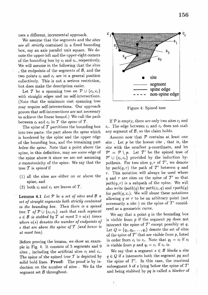
Lemma 4.1 Let $P$ be a set of sites and $B$ aset of straight segments both strictly containedin the bounding box. Then there is a spinedtree $T$ of $\mathcal{P}\cup\{c_{l}, C_{r}\}$ such that each segment$s\in B$ is stabbed by $T$ at most $2+u(s)$ timeswhere $u(s)$ denotes the number of endpoints of$s$ that are above the spine of $T$ (and hence isat most two).

Before proving the lemma, we show an exam-ple in Fig. 4. It consists of 5 segments and 9sites , including the artificial sites $c_{l}$ and $c_{r}$ .The spine of the spined tree $T$ is depicted bysolid bold lines. Proof: The proof is by in-duction on the number of sites. We fix thesegment set $\mathcal{B}$ throughout.

Figure 4: Spined tree

If $\mathcal{P}$ is empty, there are only two sites $c_{l}$ and$c_{T}$ . The edge between $c_{l}$ and $c_{r}$ does not stabany segment of $B$ , so the claim holds.

Assume now that $P$ contains at least onesite. Let $p$ be the lowest site , that is, thesite with the smallest $y$-coordinate, and let$P’=\mathcal{P}\backslash p$ . Let $T’$ be the spined tree of$P’\cup\{C_{l}, c_{r}\}$ provided by the induction hy-pothesis. For two sites $q,$ $r$ of $T’$ , we denoteby path$(q, r)$ the path of $T’$ between $q$ and$r$ . This notation will always be used where$q$ and $r$ are sites on the spine of $T’$ so thatpath $(q, r)$ is a subpath of the spine. We willalso write lpath $(q)$ for path $(c_{l,q})$ and rpath $(q)$

for path $(q, c_{r})$ . We will abuse these notationsallowing $q$ or $r$ to be an arbitrary point (notnecessarily a site) on the spine of $\mathcal{T}’$ consid-ered as a geometric curve.

We say that a point $q$ in the bounding boxis visible from $p$ if the segment $pq$ does notintersect the spine of $\mathcal{T}’$ except possibly at $q$ .Let $Q=\{q_{1}, q2, \ldots, q_{t}\}$ denote the set of sitesof the spine of $T’$ that are visible from $p$ , listedin order from $c_{l}$ to $c_{r}$ . Note that $q_{1}=c_{l}$ if $c_{l}$

is visible from $p$ and $q_{t}=c_{r}$ if $c_{r}$ is.We say that a segment $s\in B$ blocks a site

$q\in Q$ if $s$ intersects both the segment $pq$ andthe spine of $T’$ . In this case, the maximalsubsegment $b$ of $s$ lying below the spine of $T’$

and being stabbed by $pq$ is called a blocker of

156

$q$ ; we also say that $s$ supports the blocker $b$ and$b$ blocks $q$ . We call an endpoint of a blocker $b$

that is on the spine of $\mathcal{T}’$ an anchor of $b$ .Suppose $v$ is an anchor of a blocker of $q$ . We

call $v$ a right anchor of the blocker if $v$ is inrpath $(q)$ ; a left anchor if it is in lpath $(q)$ . SeeFig. 5 for pictorial illustration.

A blocker may have one anchor (left orright) or two anchors (both left and right).Note that, when a blocker has both left andright anchors, the left anchor may lie geomet-rically to the right of the right anchor, sincethe spine may not be x-monotone.

We say that two consecutive visible sites $q=$

$q_{i},$ $r=q_{i+1}$ in $Q$ and an edge $e$ in path$(q, r)$

form a good triple $(q, r, e)$ if the following threeconditions hold ( $\mathrm{s}e\mathrm{e}$ Fig. 6).

(1) $q$ and $r$ do not have a common blocker.(2) If any blocker of $r$ has a left anchor then

it is on $e$ ; if any blocker of $q$ has a rightanchor then it is also on $e$ .

(3) If $q=c_{l}$ then $e$ is incident to $c_{l}$ ; if $r=c_{r}$

then $e$ is incident to $c_{r}$ .

Figure 5: Blockers

Claim 4.2 There is at least one good triple$(q, r, e)_{f}q,$ $r\in Q,$ $e\in path(q, r)$ .

We defer the proof of the claim and firstshow how we construct the spined tree of

Figure 6: A good triple

$P\cup\{c_{l}, C\}r$ based on the claim. Let $(p, q, e)$

be a good triple in $Q$ . Our spined tree $\mathcal{T}$ isobtained from $T’$ by adding two edges $pq$ and$pr$ and removing $e$ . Since $q$ and $r$ are visiblefrom $p$ , we do not create any self-intersections,and since $e$ is in path$(q, r),$ $\tau$ remains a tree.The new spine goes through the edges $pq$ and$pr$ and it is clear that all sites are either on orabove this spine. Condition (3) ab $o\mathrm{v}\mathrm{e}$ guar-antees that $c_{l}$ and $c_{r}$ remain leaves of thetree. Therefore, $T$ is indeed a spined tree of$P\cup\{Cr’ Cr\}$ .

New stabbings are created when a segment$s\in B$ is stabbed by $pq$ or $pr$ . We considerthree cases: (a) $s$ is stabbed by both $pq$ and$pr,$ $(\mathrm{b})s$ is stabbed by $pq$ but not by $pr$ , and(c) $s$ is stabbed by $pr$ but not by $pq$ . Sincecase (c) is symmetric to case (b), we considercases (a) and (b).

In case (a), $s$ is not stabbed by any edge of$T’$ because otherwise $s$ would support a com-mon blocker of $q$ and $r$ contradicting condition(1) of a good triple. Thus, the stabbing num-ber of $s$ is two without violating the inductionhypothesis.

Next consider case (b): $s$ is stabbed by $pq$

but not by $pr$ . Let $C$ denote the closed curveformed by edges $pq,$ $pr$ and path$(q, r)$ .

157

First suppose that $s$ is not stabbed bypath$(q,r)$ . Then, one endpoint of $s$ is in theinterior of the cycle $C$ . Since the interior of $C$

is below the spine of $\mathcal{T}’$ and above the spineof $\mathcal{T}$ , the number of endpoints of $s$ above thespine ,

$\mathrm{i}\mathrm{s}$ increased by one, accounting for thenew stabbing and maintaining the inductionhypothesis.

Next suppose that $s$ is stabbed by path $(q, r)$ .This means that $s$ supports a blocker of $q$ thathas a right anchor. Condition (2) of a goodtriple implies that this right anchor lies in $e$ ,that is, $e$ is the edge in path $(q, r)$ that stabs $s$ .Since $e$ is removed in forming $\mathcal{T}$ , the induction$\mathrm{h}\mathrm{y}\mathrm{p}_{0}\mathrm{t}\square \mathrm{h}\mathrm{e}\mathrm{S}\mathrm{i}\mathrm{s}$

is maintained in this case as well.

Before we prove the claim, we introducesome more notation. Let $B$ denote the set ofall blockers (the site $p\in P$ is still fixed as thelowest site in $\mathcal{P}$ ).

For each blocker $b\in B$ and each site $q\in$

$Q$ visible from $p$ , we define a line segment$seg(q, b)$ as follows: If $b$ blocks $q$ , then $seg(q, b)$

denotes the line segment $qq’$ , where $q’$ is thepoint at which $pq$ stabs $b$ . When $b$ does notblock $q$ , we use the convention that $seg(q, b)$

is empty.

For any site $q\in Q$ visible from $p$ , we cannow introduce a partial $\mathrm{o}\mathrm{r}\mathrm{d}\mathrm{e}\mathrm{r}\prec_{q}$ on $B$ as fol-lows: $b_{1}\prec_{q}b_{2}$ if and only if $b_{1}$ and $b_{2}$ bothblock $q$ and $seg(q, b_{1})$ is properly contained in$seg(q, b_{2})$ (see Fig. 7).

Finally, we $\mathrm{d}\mathrm{e}\mathrm{f}\mathrm{i}\mathrm{n}\mathrm{e}\prec \mathrm{t}\mathrm{o}$ be the transitive clo-sure of the union of $\prec_{q}$ over all $q\in Q$ . Weclaim that $\prec$ is anti-symmetric and is there-fore indeed a partial order on $B$ . To $\mathrm{s}e\mathrm{e}$ this,consider a chain $b_{1}\prec_{q_{1}}b_{2}\prec_{q_{2}}$ .... A sim-ple induction shows that $seg(q, b_{j})$ contains$\bigcup_{1\leq i<j}Seg(q, b_{i})$ for every $q\in Q$ blocked by$b_{j}$ . Therefore, $b_{1}\prec b_{j}$ implies that $b_{j}\prec_{q}b_{1}$

does not hold for any $q$ . Therefore, $\prec \mathrm{i}\mathrm{s}$ anti-symmetric.

Figure 7: The partial order $b_{1}\prec_{q}b_{2}$ .

The following proposition will be used later.

Proposition 4.3 Let $b_{1}$ and $b_{2}$ be two block-ers with $b_{1}\prec b_{2}$ and assume that $b_{1}$ blocks$q$ . Then, the left anchor of $b_{2}$ , if any, is inlpath $(q)$ and the right anchor of $b_{2}$ , if any, $is$

in rpath$(q)$ .

Proof: of Claim 4.2. If there is no blockerthen the existence of a good triple is trivial.So assume that the set of blockers $B$ is non-empty. Without loss of generality, we may as-sume that at least one of the blockers that ismaximal with respect $\mathrm{t}\mathrm{o}\prec \mathrm{h}\mathrm{a}\mathrm{s}$ a right anchor(otherwise we argue symmetrically, swappingleft and right). Among all the maximal block-ers with a right anchor, choose the one w-hoseright anchor is the closest to $c_{r}$ in the spineof $T’$ and call it $b_{0}$ . Let $v_{0}$ denote the rightanchor of $b_{0}$ and $e$ the spine edge of $T’$ thatcontains $v_{0}$ . We define $q$ ( $r$ , resp.) to be thefirst site visible from $p$ when we traverse thespine of $\mathcal{T}’$ from $v_{0}$ towards $\mathrm{c}_{l}$ ( $c_{r}$ , resp.).

We study the three conditions of $(q, r, e)$ be-ing a good triple.

(1) $q$ and $r$ do not have a common blocker,since such a common blocker would contradictthe maximality of $b_{0}$ .

158

(2) Let $q’,$ $r’$ be the points on path $(q, r)$ suchthat path $(q^{J\prime}, r)$ is the maximal subpath ofpath $(q, r)$ that is visible from $p$ . Note that$p,q,$ $q’$ are collinear with possibly $q=q’$ and$p,r,r’$ are colinear with possibly $r=r’.$ ‘ Notetherefore that if any blocker of $q$ has a right an-chor then it is on rpath $(q’)$ and if any blockerof $r$ has a left anchor then it is on lpath $(r)’$ .

condition (2) is satisfied as long as $r=r’$ or $r$

has a blocker with a left anchor (see Fig. 9).

Figure 9: Case 2

Figure 8: Case 1

Suppose $r$ has a blocker $b$ with left anchor$v$ (see Fig. 8). Since $b_{0}$ is maximal, $b$ cannotblock $q$ . Therefore, $v$ must lie on path$(v0, r)$ .Combined with the above note, $v$ must lie onpath $(v_{0}, r^{;})$ . Since $v_{0}$ is on rpath$(q)’$ , it followsthat path( $v_{0)},$$v$ is entirely visible from $p$ . Thisin turn implies that $v_{0}$ and $v$ are on the samespine edge, namely $e$ . This establishes the firsthalf of condition (2). For the second half, thatis the condition that the right anchor of anyblocker of $q$ lies in $e$ , first note that the max-imality of $b_{0}$ , combined with the above note,implies that any such right anchor must lie onpath ($q’,$ $v_{0)}$ . Thus, if $q’$ is on $e$ , we are done.So suppose $q’$ is not on $e$ . This implies that$e$ lies entirely within path$(rr)’,$ . Therefore wemust have $r\neq r’$ in this case. Moreover, $r$ doesnot have a blocker with a left anchor since anysuch anchor must lie on path $(v0, \Gamma)\cap lpath(r)’$ ,which is empty in this case. We conclude that

(3) If $q=c_{l}$ then $e$ is incident to $c_{l}$ becauseit is impossible for the spine edge incident to$c_{l}$ to be invisible from $p$ in the neighborhoodof $c_{l}$ while $c_{I}$ is visible. If $r=c_{r}$ then $e$ isincident to $c_{r}$ for an analogous reason.

To deal with the remaining case where con-dition (2) may not be satisfied by the triple$(q, r, e)$ , suppose that $r\neq r’$ and that $r$ doesnot have a blocker with a left anchor. In thiscase, the last edge of path $(v\mathrm{o}, r)$ is invisiblefrom $p$ so that the first edge $f$ of rpath $(r)$ isvisible from $p$ at least locally at $r$ . Let $w$ bethe next visible site in the spine of $T’$ after$r$ . We claim that $(r,w, f)$ is a good triple (seeFig. 9).

We first argue that $r$ does not have a blockerat all. Suppose $r$ did have a blocker $b$ . Let $b^{*}$

be the maximal blocker such that $b\prec b^{*}$ . If$b^{*}$ had a right anchor, then by Proposition 4.3this anchor would have to be in rpath$(r)$ , con-tradicting the choice of $b_{0}$ . Therefore, $b^{*}$ musthave a left anchor $u$ . By Proposition 4.3 again,$u$ must lie on lpath $(r)$ . However, $u$ cannotlie on $l_{\mathrm{P}^{a}}th(v_{0})$ because this would contradictthe maximality of $b_{0}$ . Therefore, $u$ must lie

159

on path $(v0, r)$ , but this implies that $b^{*}$ is ablocker of $r$ with a left anchor, contradictingour assumption. Therefore, $r$ does not havea blocker at all. This trivially implies that $r$

and $w$ do not have a common blocker, con-dition (1) of $(r, w, f)$ being a good triple. Forcondition (2) we need only consider blockers of$w$ with left anchors. Since $f$ is the only edge inpath$(r,w)$ that has a part visible from $p$ and$f$ is incident to $r$ , such left anchors must alllie on $f$ . Finally, a reasoning analogous to theone for $(q, r, e)$ shows that the triple

$(r, w,f)\square$

satisfies condition (3).

Now we come to our main theorem.

Theorem 4.4 Givena set $B$ of non-intersecting line segments anda set $P$ of sites in the $plane_{)}$ there is alwaysa straight-edge spanning tree of $\mathcal{P}$ that stabseach line segment of $B$ at most 4 times.

Proof: We first compute a bounding boxthat properly contains all the objects of $B$

and $P$ . Let $c_{l}$ and $c_{r}$ be the upper-left andupper-right corners of the bounding box, re-spectively. Then, applying the lemma to $B$

and $P\cup\{C_{l}, c_{r}\}$ , we obtain a spined tree $\mathcal{T}$ .Removing the artificial sites $c_{l}$ and $c_{r}$ from $\mathcal{T}$ ,it remains a tree since $c_{l}$ and $c_{r}$ are leaves of$T$ . It follows from the statement of the lemmathat the resultant tree is a spanning tree over$\prime p$ that stabs each line segment of $B$ at most 4times. $\square$

5 ConclusionsIn this paper we have studied spanning treesamong $n$ points whose edges cross few among agiven set of $m$ barriers. When the barriers aredisjoint, near-linear bounds for the cost of sucha tree can be obtained by several simple argu-ments. Using more sophisticated techniques,we were able to show that a linear cost span-ning tree is possible in many cases.

One of the techniques we used is the con-struction of certain BSPs on the barriers. This

raises the question of whether our other meth-ods, by ‘reverse-engineering,’ can help resolvesome open questions about BSPs, includingthe long-standing one about the existence of alinear space BSP for disjoint line segments inthe plane.

We note that the number of barriers crossedby linking two points is not a distance func-tion and does not satisfy the triangle inequal-ity. This means that the existence of otherlow-cost structures among the points, such asHamiltonian tours and matchings, remains aninteresting research problem.

References[1] M. de Berg. Linear size binary space parti-

tions for uncluttered scenes. Technical Re-port UU-CS-1998-12, Utrecht University,1998

[2] M. de Berg, M. J. Katz, A. F. van derStappen, and J. Vleugels. Realistic in-put models for geometric algorithms. InProc. 13th Annu. ACM Sympos. Comput.Geom., 294-303, 1997

[3] F. d’Amore and P. G. Franciosa. On theoptimal binary plane partition for sets ofisothetic rectangles. Inform. Process. Lett.,44:255-259, 1992

[4] H. Edelsbrunner, L. J. Guibas, andJ. Stolfi. Optimal point location in amonotone subdivision. SIAM J. Comput.,$15(2):317- 340$ , 1986

[5] M. S. Paterson and F. F. Yao. Efficientbinary space partitions for hidden-surfaceremoval and solid modeling. Discrete Com-put. Geom., 5:485-503, 1990

[6] J. Snoeyink and M. van Kreveld. Linnear-time reconstruction of Delaunay trian-gulations with applications. In Proc.Annu. European Sympos. A lgorithms, Lec-ture Notes in Computer Science 1284, 459-471, Springer-Verlag, 1997.

160