Cross Slope Collection using Mobile Lidar - ACEC of...
80
Cross Slope Collection using Mobile Lidar December 2, 2015 ACEC/SCDOT Annual Meeting
Transcript of Cross Slope Collection using Mobile Lidar - ACEC of...

Cross Slope Collection using Mobile Lidar
December 2, 2015 ACEC/SCDOT Annual Meeting

Adequate cross slopes on South Carolina Interstates result in: • Proper drainage • Enhance driver safety by reducing the potential for hydroplaning.
SCDOT is seeking to have an efficient method for collecting interstate cross slope data so that an accurate and comprehensive cross slope database can be maintained.
Mobile Scanning to collect accurate cross slope data on South Carolina interstates. save over 90% of the cost on cross-slope verification reduce four to six months of contract time for each interstate rehabilitation
project.
Introduction

• Comprehensive technical and economic evaluation of multiple mobile scanning systems in terms of the accuracy and precision of collected cross slope data
• Procedures to calibrate, collect, and process this data.
Project team • Dr. Wayne A. Sarasua, P.E. • Dr. Jennifer H. Ogle • Dr. Brad Putman • Dr. Ronnie Chowdhury, P.E.
• Dr. W. Jeffrey Davis
Department of Civil Engineering Clemson University
The Citadel
Research Approach

1. Perform technical and economic comparisons of the alternative mobile scanning technologies and conventional survey methods for cross slope verification
2. Establish a validation site that contains tangent and curve sections using traditional survey methods that may then be used to qualify mobile scanning vendors;
3. Establish SCDOT guidelines for testing procedures and data delivery for the vendor rodeo and ultimately statewide data collection; and
4. Provide a survey of the cross slope and other related geometric properties for the entire interstate system in South Carolina with the selected technology which is suitable for future reference on projects.
Objectives
a normal cross slope in South Carolina is 2.08 percent with some exceptions depending on the number of lanes
Relatively flat pavement cross-slopes of less than one percent (1%) are prone to creating unacceptable water depths
Cross slopes that are too steep can cause vehicles to drift and become unstable when crossing over the crown to change lanes.
Typical Cross-slope
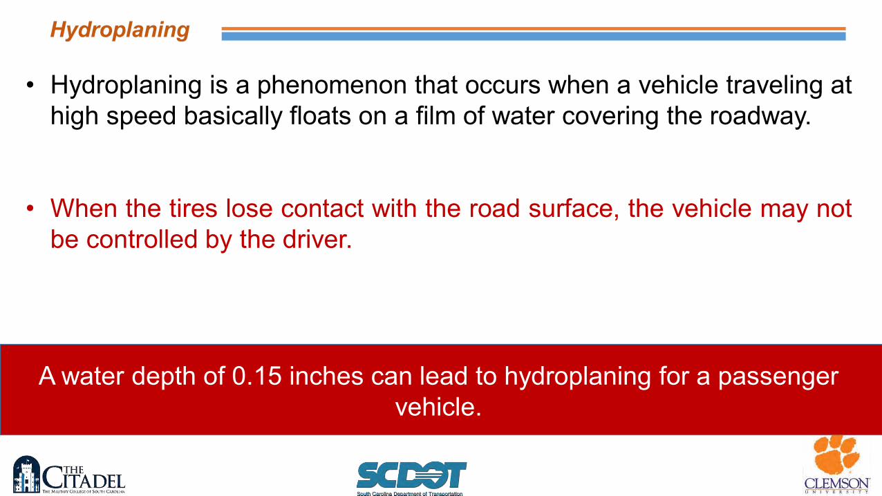
• Hydroplaning is a phenomenon that occurs when a vehicle traveling at high speed basically floats on a film of water covering the roadway.
• When the tires lose contact with the road surface, the vehicle may not be controlled by the driver.
A water depth of 0.15 inches can lead to hydroplaning for a passenger vehicle.
Hydroplaning
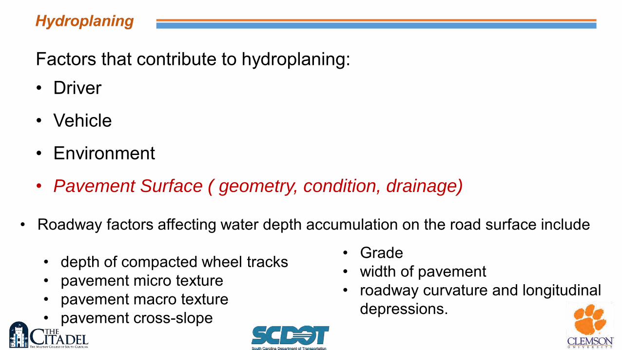
Factors that contribute to hydroplaning: • Driver
• Vehicle
• Environment
• Pavement Surface ( geometry, condition, drainage)
• Roadway factors affecting water depth accumulation on the road surface include
• depth of compacted wheel tracks • pavement micro texture • pavement macro texture • pavement cross-slope
• Grade • width of pavement • roadway curvature and longitudinal
depressions.
Hydroplaning
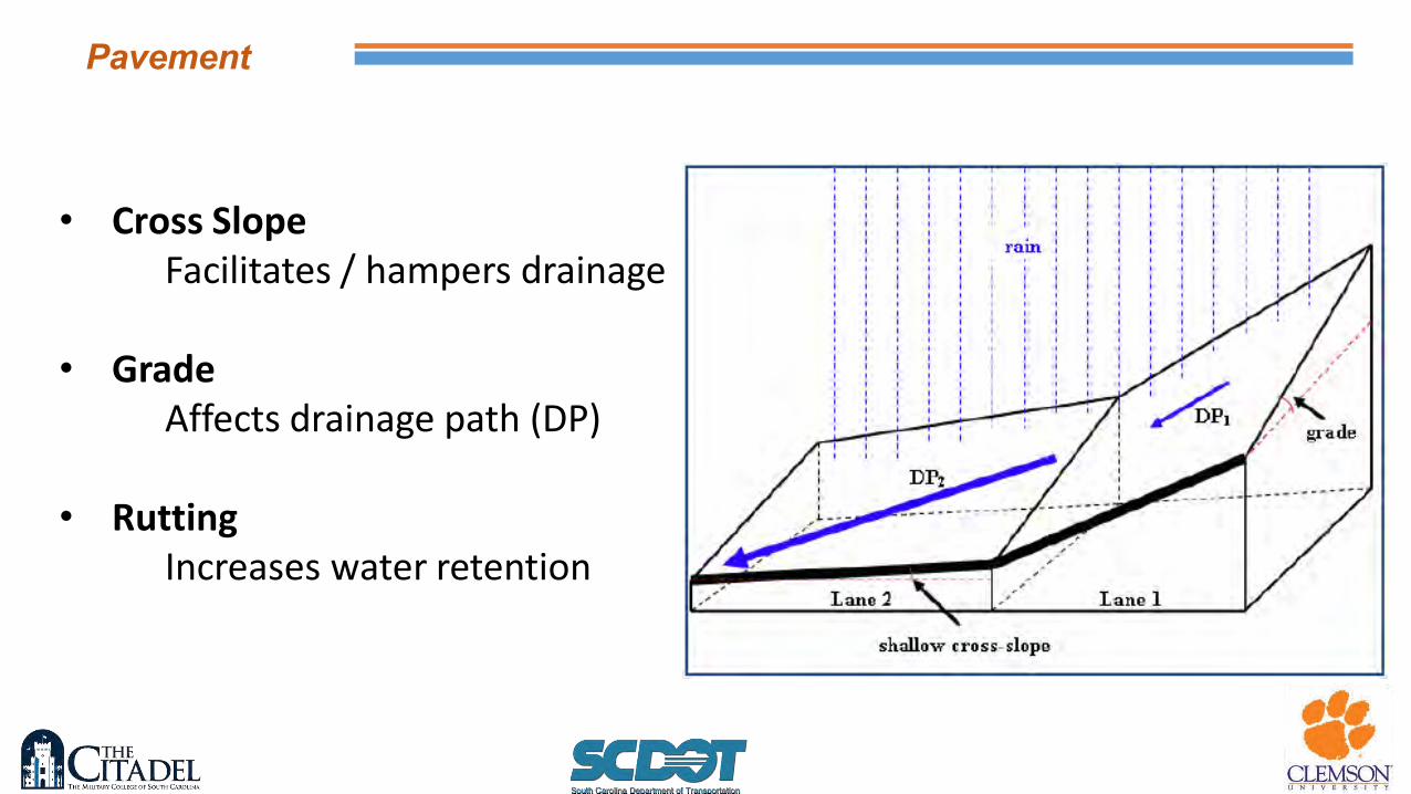
• Cross Slope
Facilitates / hampers drainage
• Grade Affects drainage path (DP)
• Rutting
Increases water retention
Pavement
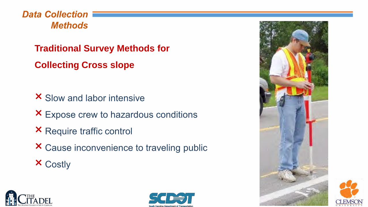
Traditional Survey Methods for
Collecting Cross slope
× Slow and labor intensive
× Expose crew to hazardous conditions
× Require traffic control
× Cause inconvenience to traveling public
× Costly
Data Collection Methods
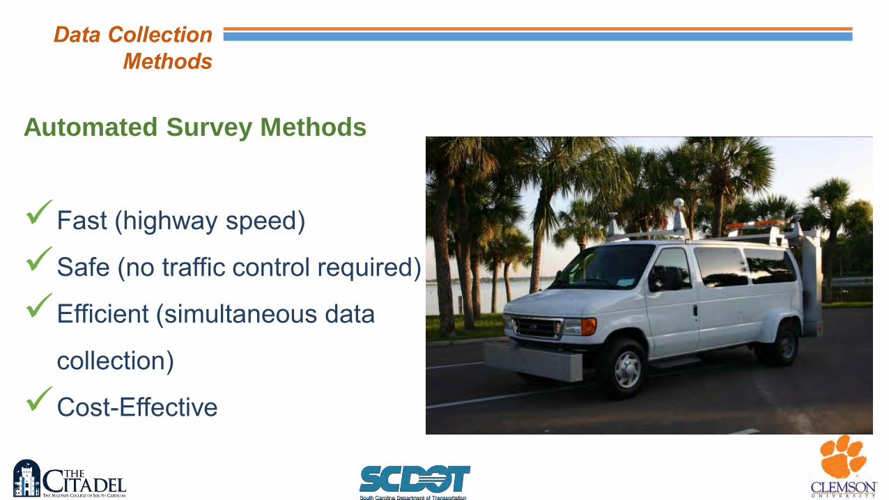
Automated Survey Methods
Fast (highway speed)
Safe (no traffic control required)
Efficient (simultaneous data
collection)
Cost-Effective
Data Collection Methods
The SCDOT’s cross slope verification specification is included in the Supplemental Specification updated on November 16, 2009
Contractor is responsible for obtaining the existing cross slope data • collecting elevation data for the edge of each travel lane
• Even 100-ft stations in tangents • Even 50-ft stations in curves.
Elevation data shall be recorded in accordance with the SCDOT Preconstruction
Survey Manual (2012) to the nearest 0.01 ft.
SCDOT’s cross slope verification specification

The elevation data shall be collected at the edge of each travel lane at
1. minimum of one random location every 300 ft. in tangent sections
2. beginning and end of super elevation, flat cross slopes within the
super elevation transition, and beginning and end of maximum super elevation
3. cross slopes at beginning and end of bridges.
SCDOT’s cross slope verification specification

The SCDOT has two acceptable tolerance levels for cross slopes: Tolerance Level 1: ± 0.00174 ft/ft (± ¼ in over 12 ft or ± 0.174%) of the design cross slope Tolerance Level 2: ± 0.00348 ft/ft (± ½ in over 12 ft or ± 0.348%) of the design cross slope When final measurements is :
• Within Tolerance Level1: no pay adjustments for the work.
• Outside of Tolerance Level 1: either corrective measures may be required at the
contractor’s expense or a pay reduction will be assessed to the work. • outside of Tolerance Level 2: the work will either be corrected at the contractor’s
expense or work will be subject to a pay reduction
SCDOT’s cross slope verification specification

These guide specifications provide a template that can be adopted by
state DOTs when developing or modifying their pavement performance
specification documents.
the SHRP2 guide specification includes a target value of ± 0.2% of the
design value for the final measurement after project completion.
SHRP2 Pavement Performance Specification

AASHTO PP70-10 recommend the following minimums: • Interval between transverse profiles
• <10-ft for network-level collection • <1.5-ft for project-level collection.
• The transverse profile width
• >13-ft for distress detection • >14-ft if edge drop-off is desired.
• The data points in the transverse profile are to be no more than 0.4-in apart. • The resolution of the vertical measurements is to be no greater than 0.04-in
AASHTO Transverse Profile Measurement Standard of Practice

The cross slope specifications in many states are similar to those of the SCDOT with most having a single tolerance level of approximately 0.2% from the design cross slope. While the specifications may be similar, the methods used to measure the cross slope do vary.
State Method Frequency Tolerance
Florida Electronic level with a length of 4-ft and accuracy of 0.1o
Tangents: 100-ft Superelevation: 100-ft
± 0.2% (average deviation) and ± 0.4% (individual deviation) for tangent and superelevation
Alabama Straight edge 10-ft long
Not specified ± 0.3% for tangents and superelevations
Other states cross slope verification specification
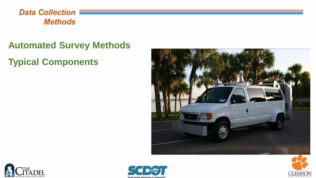
Automated Survey Methods
Typical Components
Data Collection Methods
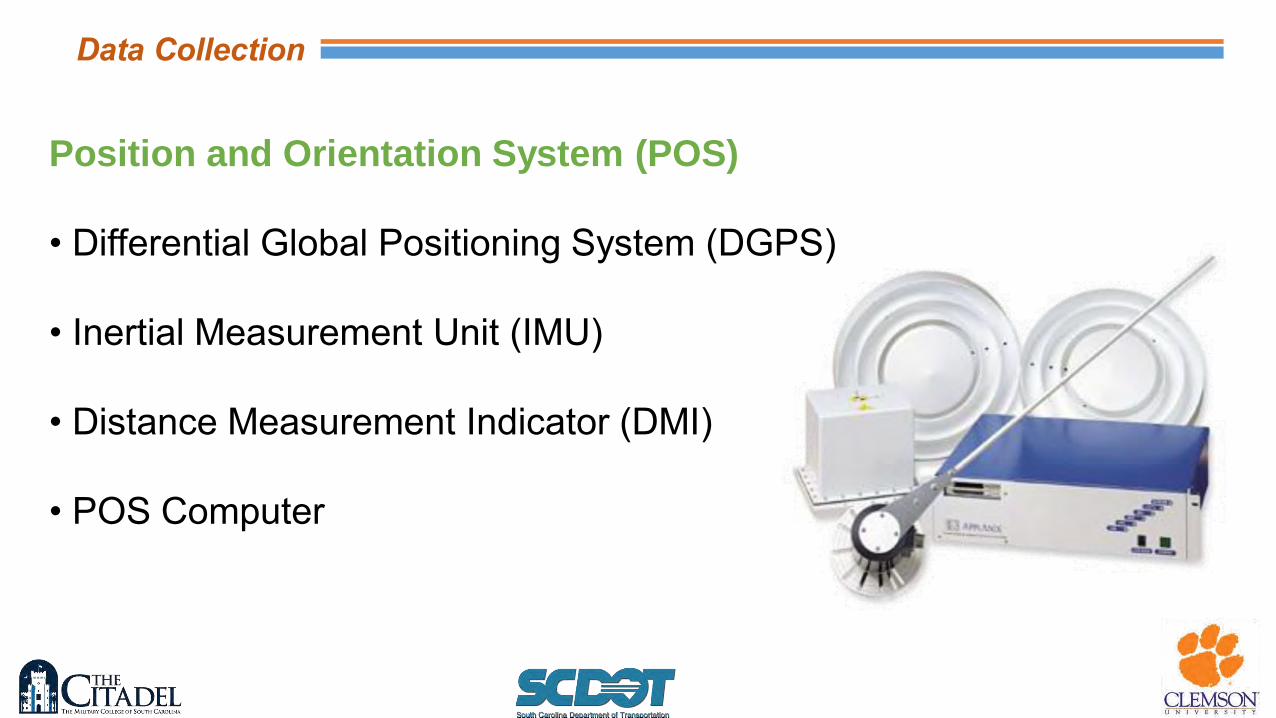
Position and Orientation System (POS)
• Differential Global Positioning System (DGPS)
• Inertial Measurement Unit (IMU)
• Distance Measurement Indicator (DMI)
• POS Computer
Data Collection
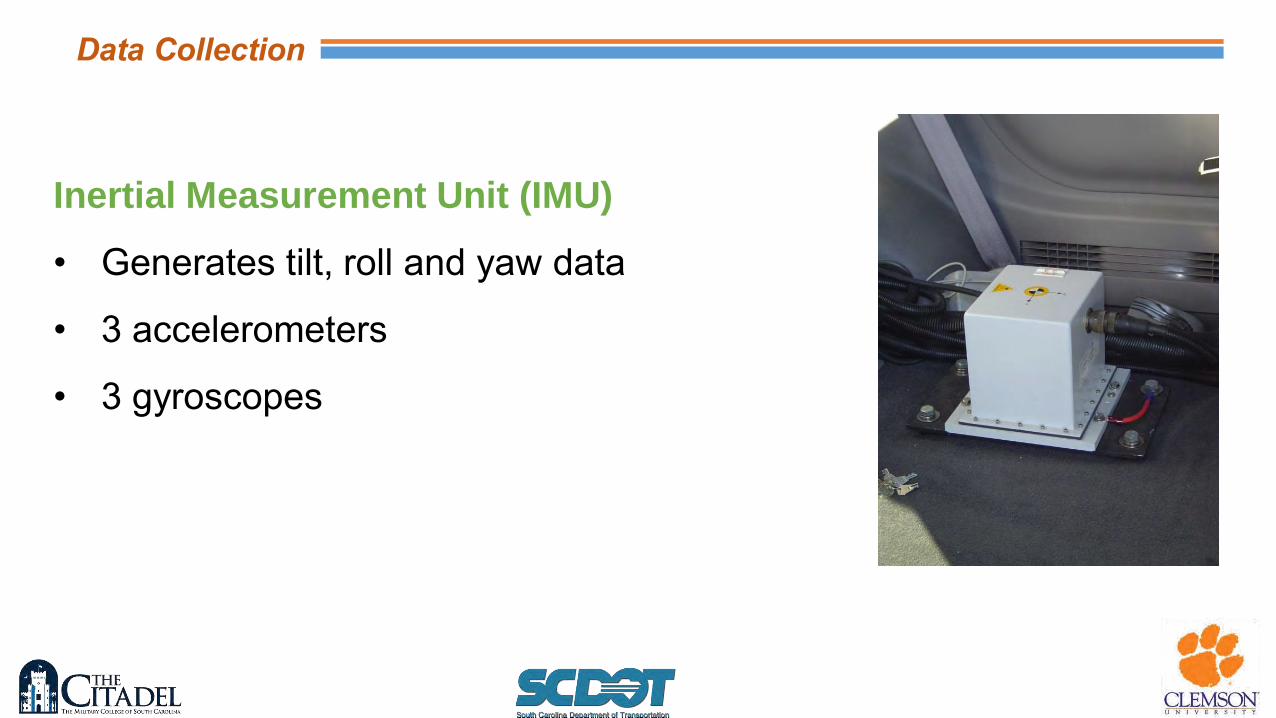
Inertial Measurement Unit (IMU)
• Generates tilt, roll and yaw data
• 3 accelerometers
• 3 gyroscopes
Data Collection
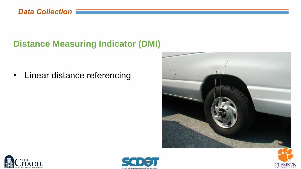
Distance Measuring Indicator (DMI)
• Linear distance referencing
Data Collection
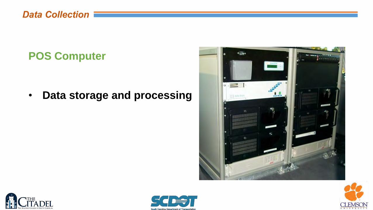
POS Computer
• Data storage and processing
Data Collection
Stand Alone Gyroscope System Vehicle mounted subsystem that utilizes a combination of gyroscopes that record vehicle pitch, roll, and heading at traffic speeds. The data collected from the gyroscopes can be interpreted by accompanying software to determine pavement cross slope at approximately 13-ft intervals.
Other systems combine sensitive gyroscopes and accelerometers to collect precise vehicle roll data. When this data is coupled with GPS and a supplemental distance measurement system, the transverse profile data can be used to determine the pavement cross slope at rod and level accuracy.
Automated Mobile Transverse Profile Data Collection Methods
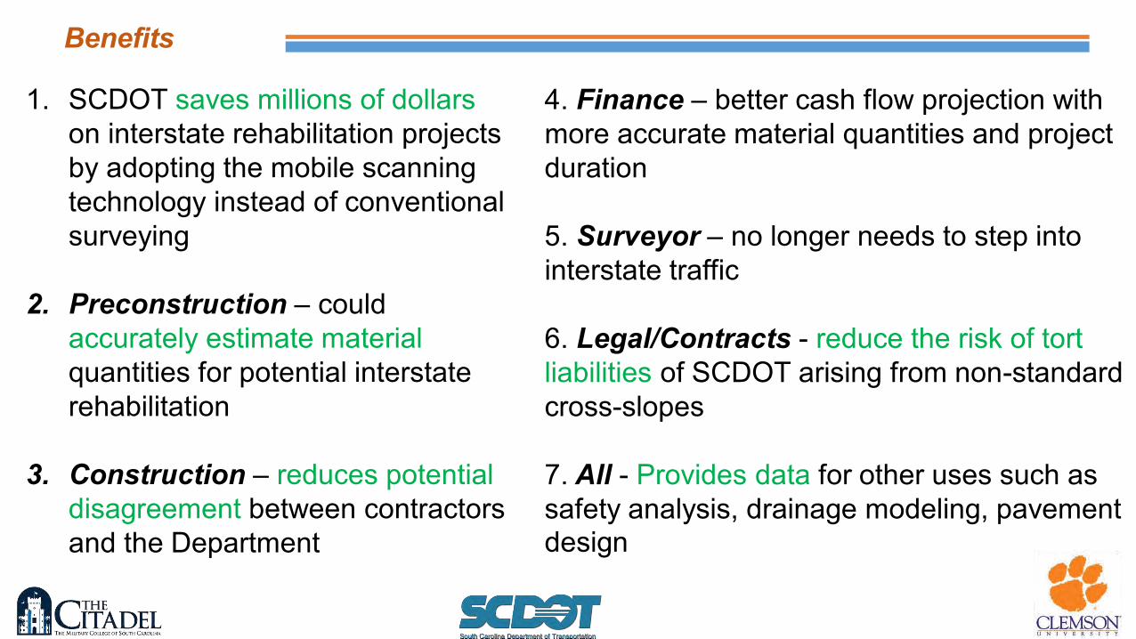
1. SCDOT saves millions of dollars on interstate rehabilitation projects by adopting the mobile scanning technology instead of conventional surveying
2. Preconstruction – could accurately estimate material quantities for potential interstate rehabilitation
3. Construction – reduces potential disagreement between contractors and the Department
Benefits
4. Finance – better cash flow projection with more accurate material quantities and project duration 5. Surveyor – no longer needs to step into interstate traffic 6. Legal/Contracts - reduce the risk of tort liabilities of SCDOT arising from non-standard cross-slopes 7. All - Provides data for other uses such as safety analysis, drainage modeling, pavement design

Additional Literature
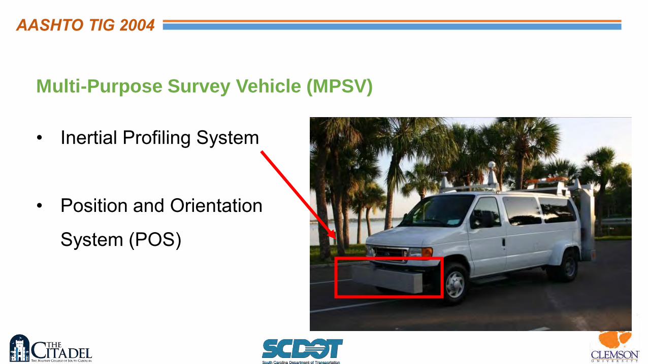
• Inertial Profiling System
• Position and Orientation
System (POS)
Multi-Purpose Survey Vehicle (MPSV)
AASHTO TIG 2004
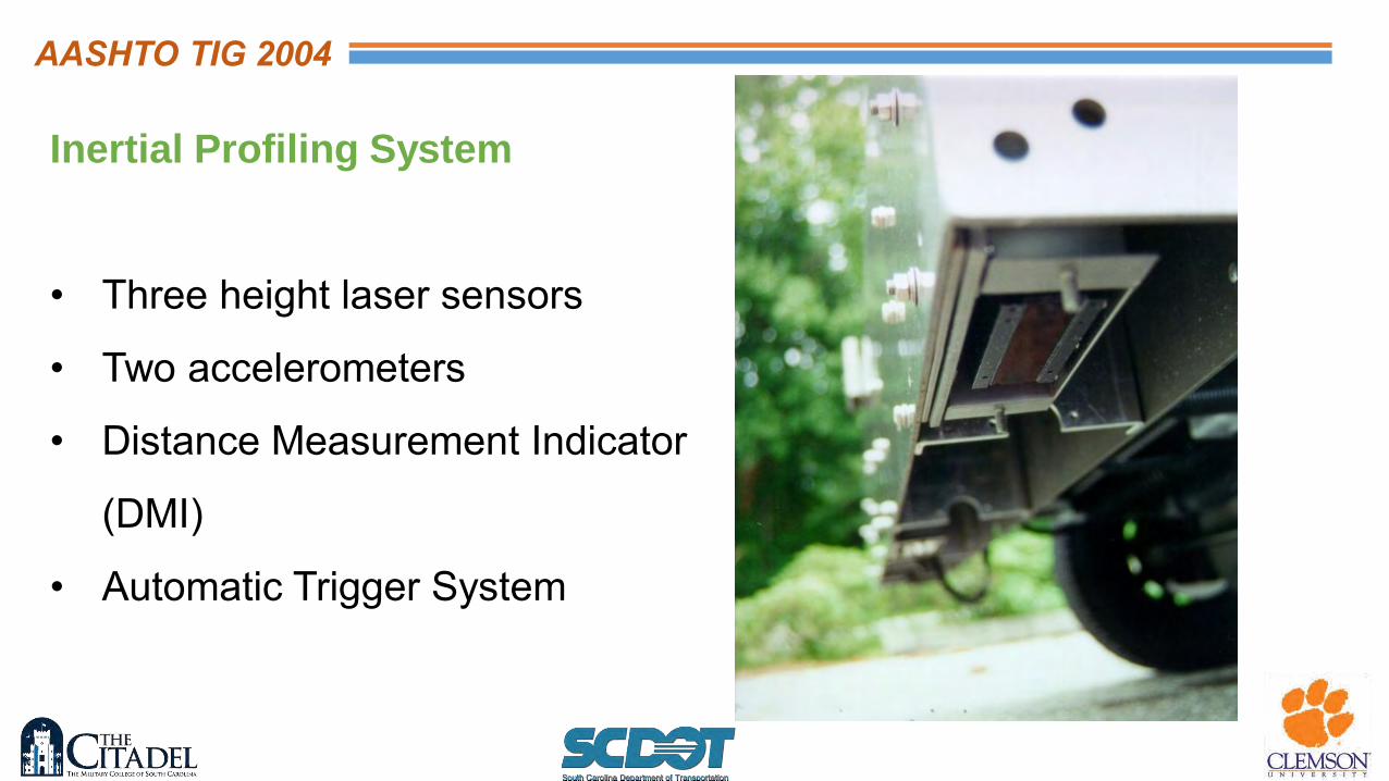
Inertial Profiling System
• Three height laser sensors
• Two accelerometers
• Distance Measurement Indicator
(DMI)
• Automatic Trigger System
AASHTO TIG 2004

http://aii.transportation.org/Documents/PaveSuite/acdp-presentation.pdf
Automated Cross-Slope Analysis Program (ACAP)
• Imports MPSV data
• Calculates cross-slope, grade, rutting, distance)
• Calculates drainage path length
• Generates outputs (tabular and graphical)
AASHTO TIG
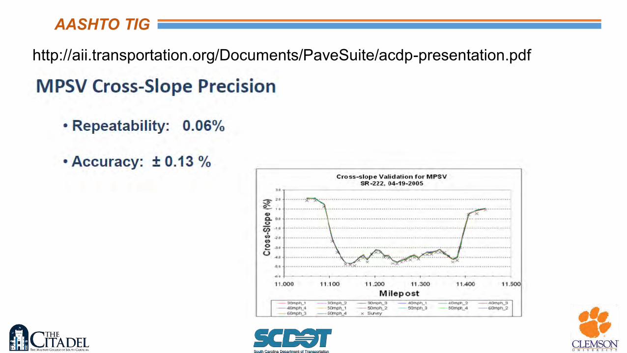
http://aii.transportation.org/Documents/PaveSuite/acdp-presentation.pdf
AASHTO TIG

AASHTO TIG
AASHTO TIG
AASHTO TIG
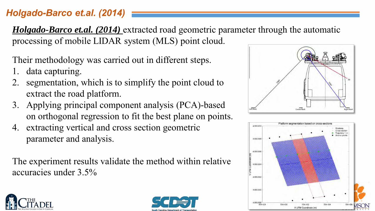
Their methodology was carried out in different steps. 1. data capturing. 2. segmentation, which is to simplify the point cloud to
extract the road platform. 3. Applying principal component analysis (PCA)-based
on orthogonal regression to fit the best plane on points. 4. extracting vertical and cross section geometric
parameter and analysis. The experiment results validate the method within relative accuracies under 3.5%
Holgado-Barco et.al. (2014) extracted road geometric parameter through the automatic processing of mobile LIDAR system (MLS) point cloud.
Holgado-Barco et.al. (2014)
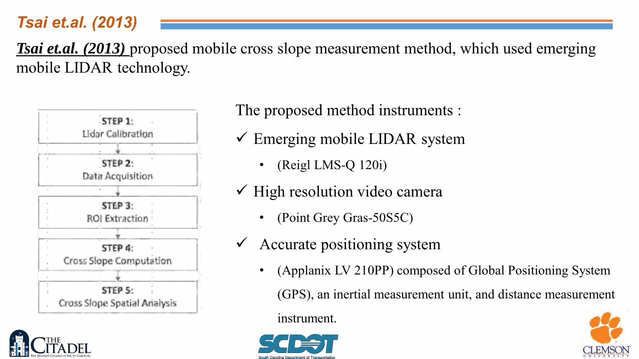
Tsai et.al. (2013) proposed mobile cross slope measurement method, which used emerging mobile LIDAR technology.
The proposed method instruments :
Emerging mobile LIDAR system • (Reigl LMS-Q 120i)
High resolution video camera • (Point Grey Gras-50S5C)
Accurate positioning system • (Applanix LV 210PP) composed of Global Positioning System
(GPS), an inertial measurement unit, and distance measurement
instrument.
Tsai et.al. (2013)

Data Acquisition with LIDAR
Region of Interest Extraction
Tsai et.al. (2013)
The results showed the proposed method achieved desirable accuracy
Maximum difference of 0.28% cross slope (0.17°)
Average difference of less than 0.13% cross slope (0.08°) from the digital auto level
measurement.
Standard deviations within 0.05% (0.03°) at 15 benchmarked locations in three runs.
The acceptable accuracy is typically 0.2% (or 0.1°) during construction quality control.
The case study on I-285 demonstrated that the proposed method can efficiently conduct network-level analysis. The GIS-based cross slope measurement map of the 3-miles section of studied roadway can be derived in fewer than 2 person hours with use of the collected raw LIDAR data Front pointing laser is multi-purpose
Tsai et.al. (2013)
Sourleyrette et al. (2003) attempted to collect grade and cross slope from LIDAR data on
tangent highway sections.
The measurements were compared against autolevel data collection for 10 test sections
along Iowa Highway 1.
The physical boundaries of shoulders and lanes were determined by visual inspection from
(a) 6-in resolution ortho-photos
(b) 12-in ortho-photo by Iowa DOT
(c) triangular irregular network (TIN) from LIDAR.
Sourleyrette et al. (2003)
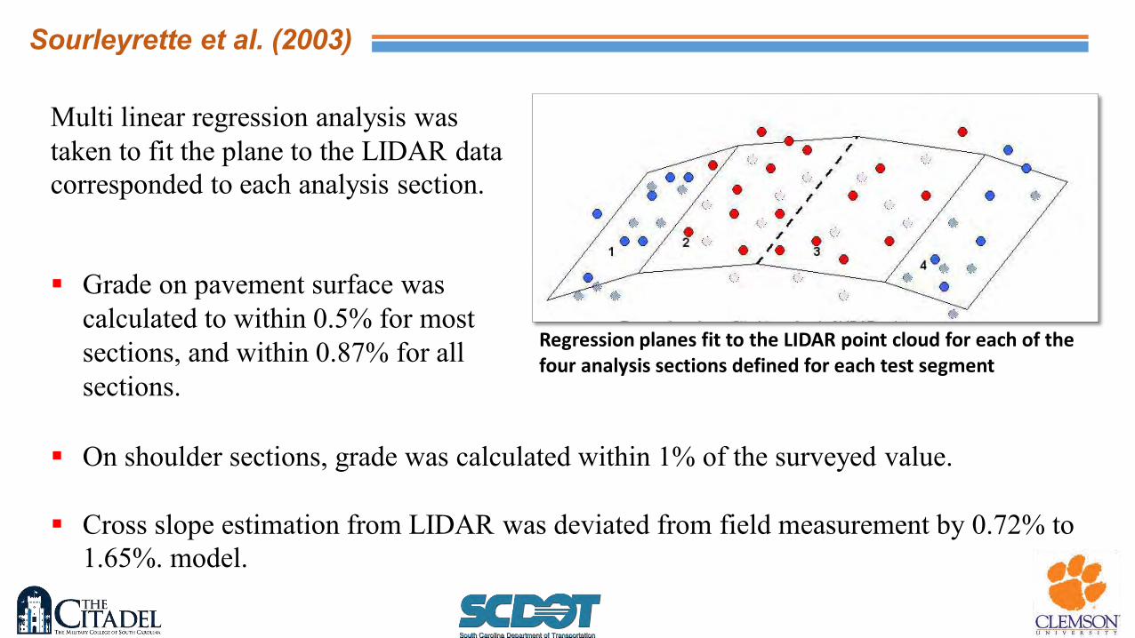
Multi linear regression analysis was taken to fit the plane to the LIDAR data corresponded to each analysis section.
Regression planes fit to the LIDAR point cloud for each of the four analysis sections defined for each test segment
Grade on pavement surface was calculated to within 0.5% for most sections, and within 0.87% for all sections.
On shoulder sections, grade was calculated within 1% of the surveyed value.
Cross slope estimation from LIDAR was deviated from field measurement by 0.72% to 1.65%. model.
Sourleyrette et al. (2003)
Zhang and Frey (2012)
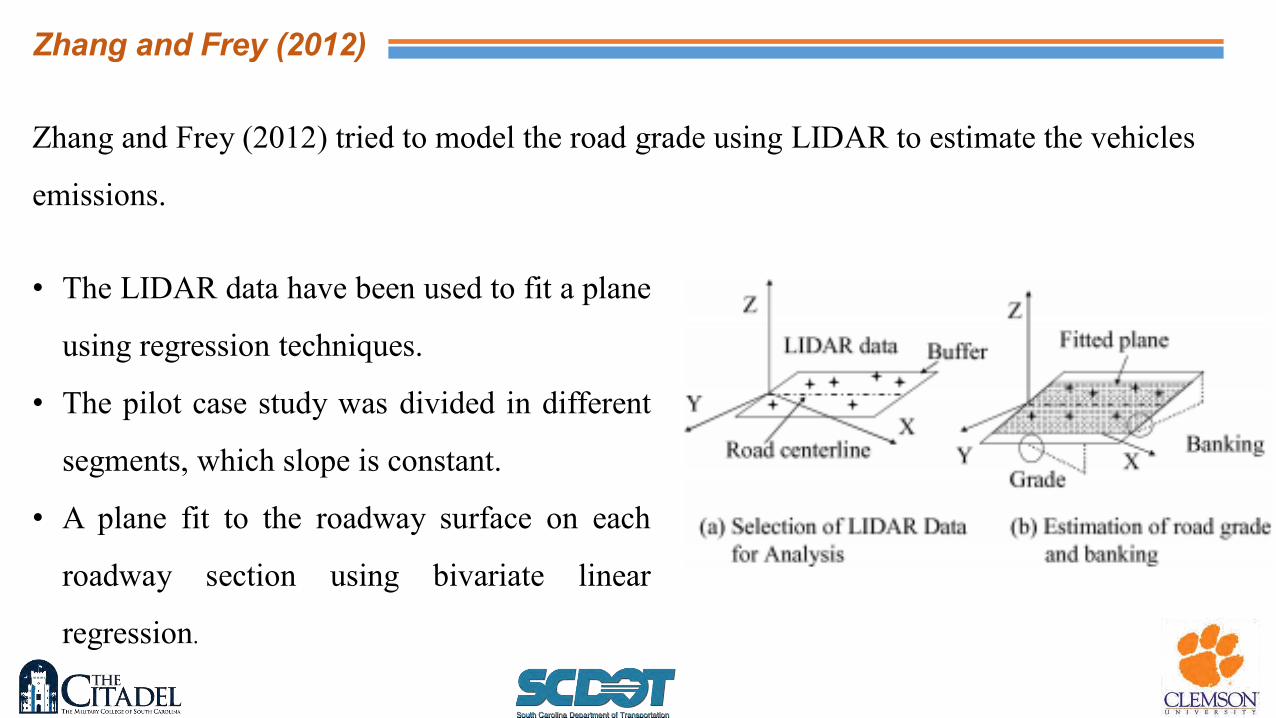
Zhang and Frey (2012) tried to model the road grade using LIDAR to estimate the vehicles
emissions.
• The LIDAR data have been used to fit a plane
using regression techniques.
• The pilot case study was divided in different
segments, which slope is constant.
• A plane fit to the roadway surface on each
roadway section using bivariate linear
regression.

Jaakkola et al. (2008) discussed that laser-based mobile mapping is necessary for
transportation study due to the huge amount of data produced.
• The data was collected with the Finnish Geodetic Institute (FGI) Roamer mobile
mapping system (MMS).
Part of the point cloud
Jaakkola et al. (2008)
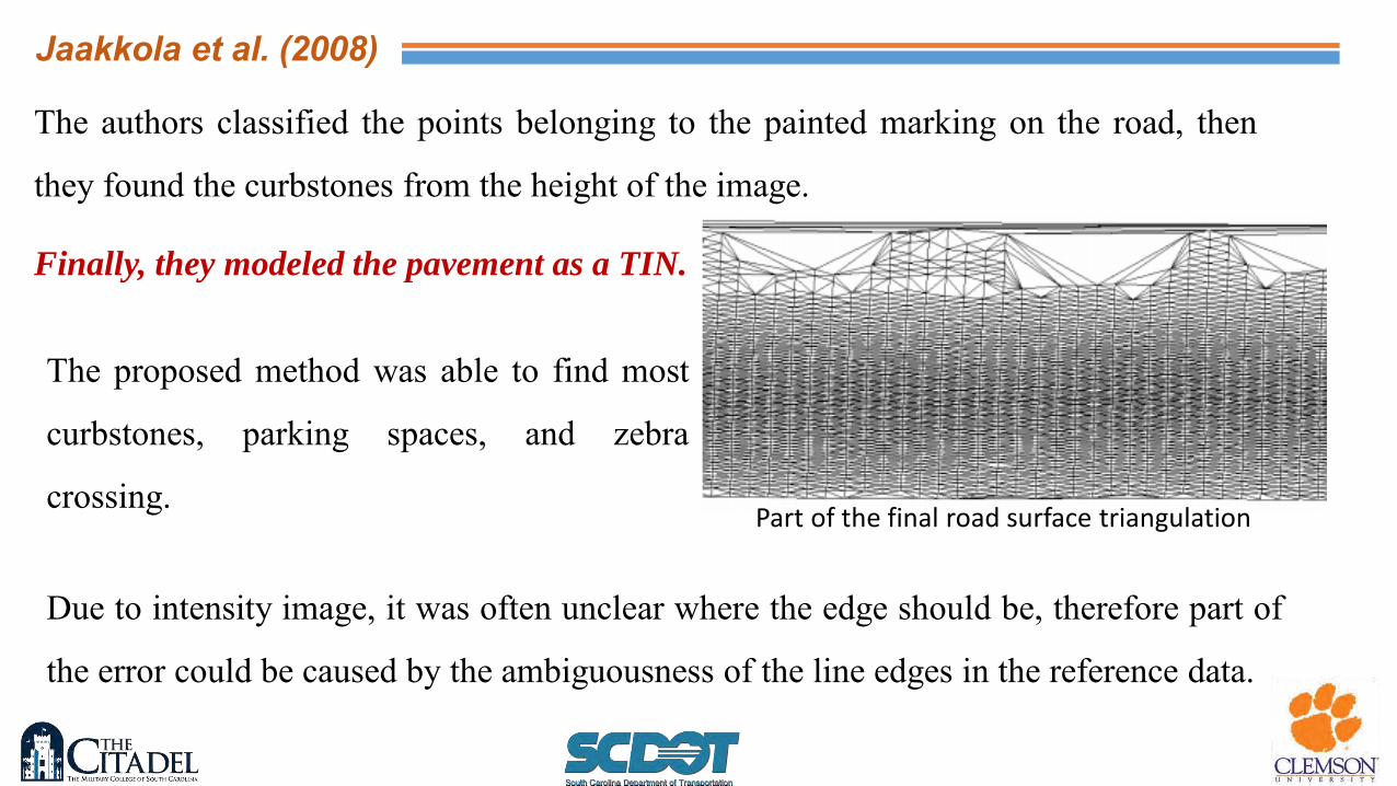
The authors classified the points belonging to the painted marking on the road, then
they found the curbstones from the height of the image.
Finally, they modeled the pavement as a TIN.
The proposed method was able to find most
curbstones, parking spaces, and zebra
crossing. Part of the final road surface triangulation
Due to intensity image, it was often unclear where the edge should be, therefore part of
the error could be caused by the ambiguousness of the line edges in the reference data.
Jaakkola et al. (2008)
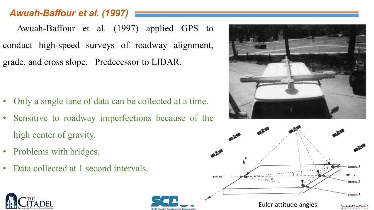
Awuah-Baffour et al. (1997) applied GPS to
conduct high-speed surveys of roadway alignment,
grade, and cross slope. Predecessor to LIDAR.
• Only a single lane of data can be collected at a time.
• Sensitive to roadway imperfections because of the
high center of gravity.
• Problems with bridges.
• Data collected at 1 second intervals.
Euler attitude angles.
Awuah-Baffour et al. (1997)

Gathering precise positional data
is corresponded to
• roadway measurement
• differential correction with GPS
base station at fixed points.
Comparison of GPS and surveying grade data collection
Large volume data can be collected in a
short period of time while a data
collection vehicle travel in the
highways
Awuah-Baffour et al. (1997)
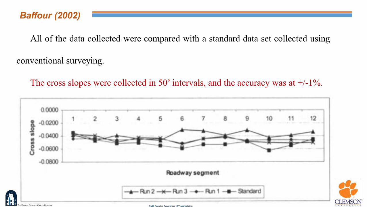
All of the data collected were compared with a standard data set collected using
conventional surveying.
The cross slopes were collected in 50’ intervals, and the accuracy was at +/-1%.
Baffour (2002)

Potential Benefit Over LIDAR is that extensive post-processing is not required to
acquire cross slope data.
Problem with using a dual RTK GPS system is loss of lock when traveling under
bridges.
An inertial device doesn’t have this problem.
LIDAR can collect data over multiple lanes with a single pass.
GPS with an Attitude

Clemson’s Mobile Laboratory
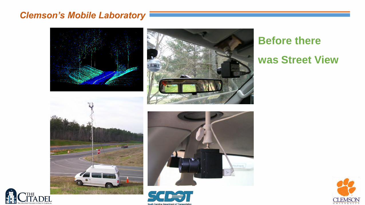
Clemson’s Mobile Laboratory
Before there
was Street View
Clemson’s Mobile Laboratory
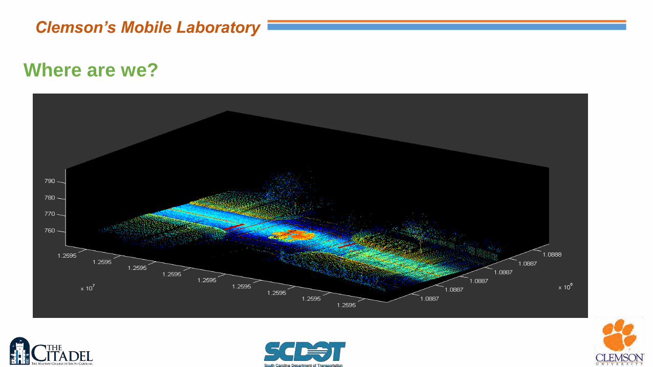
Where are we?
Clemson’s Mobile Laboratory
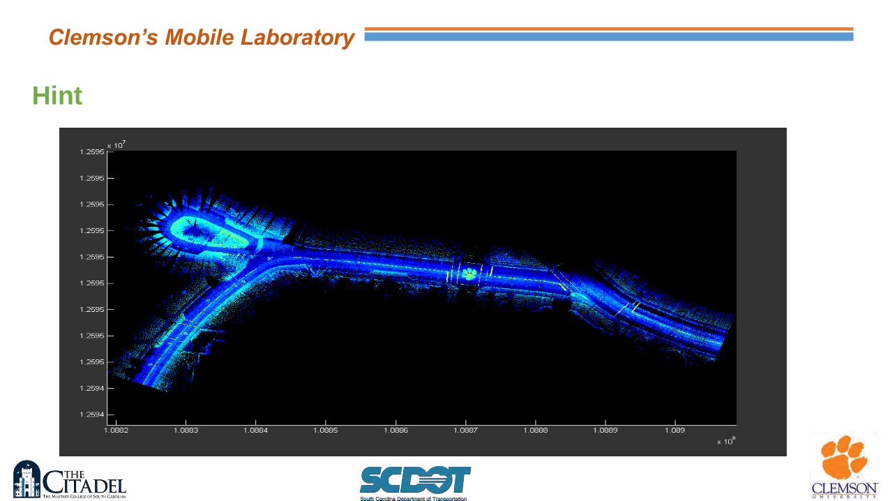
Hint


Clemson’s Mobile Laboratory
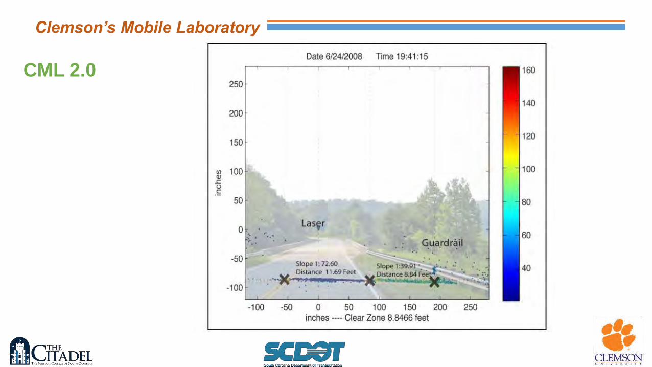
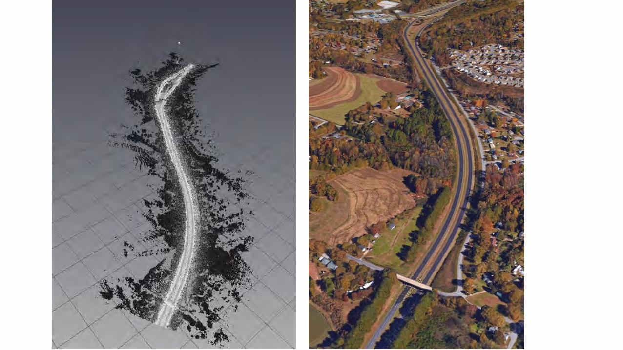
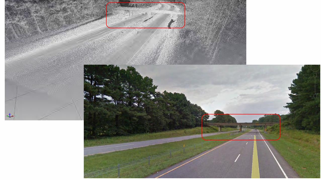
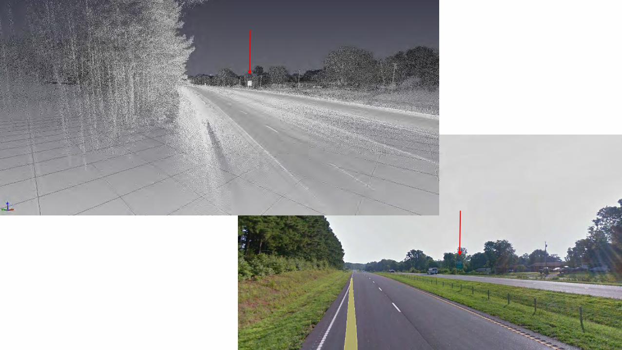
CML 2.0
US 123
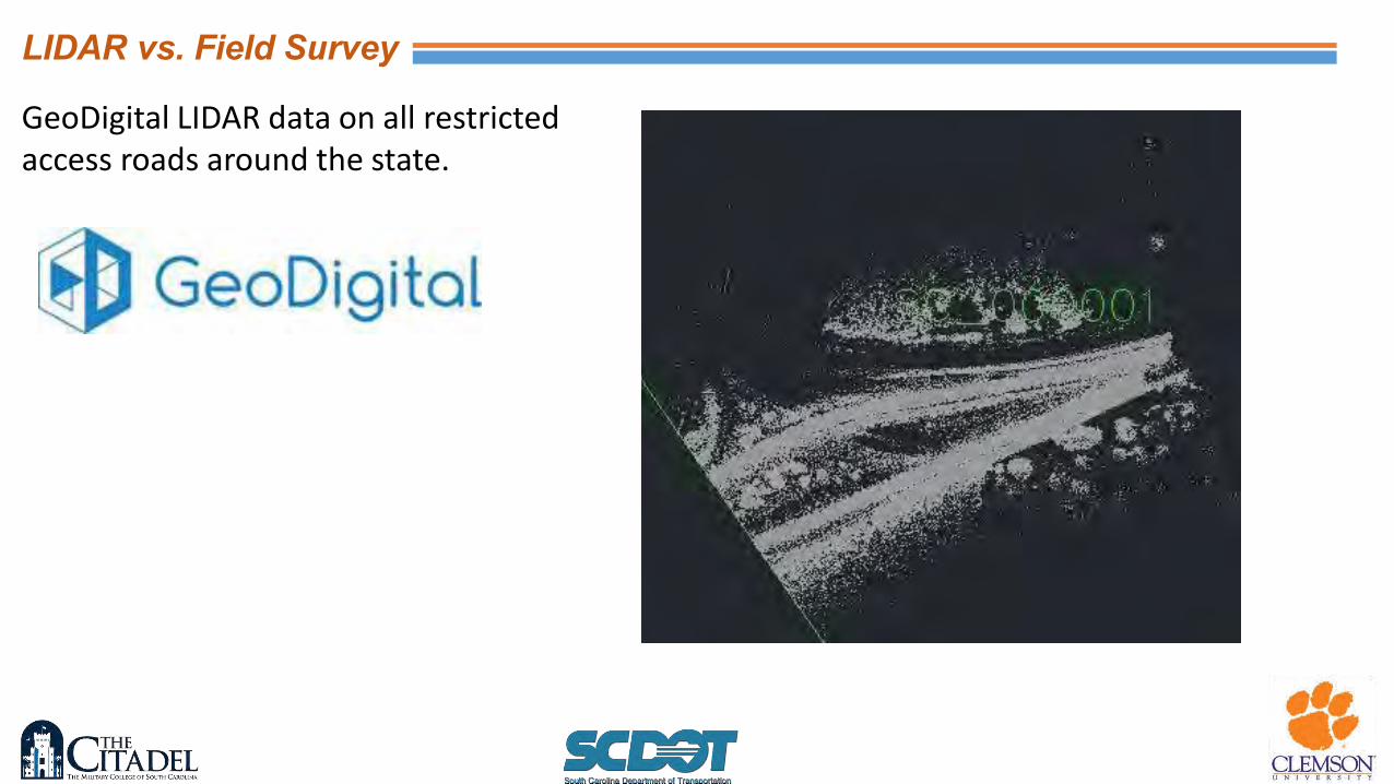
Ross Ave GeoDigital LIDAR data on all restricted access roads around the state.
LIDAR vs. Field Survey
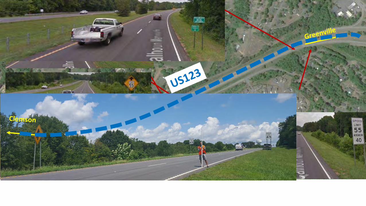
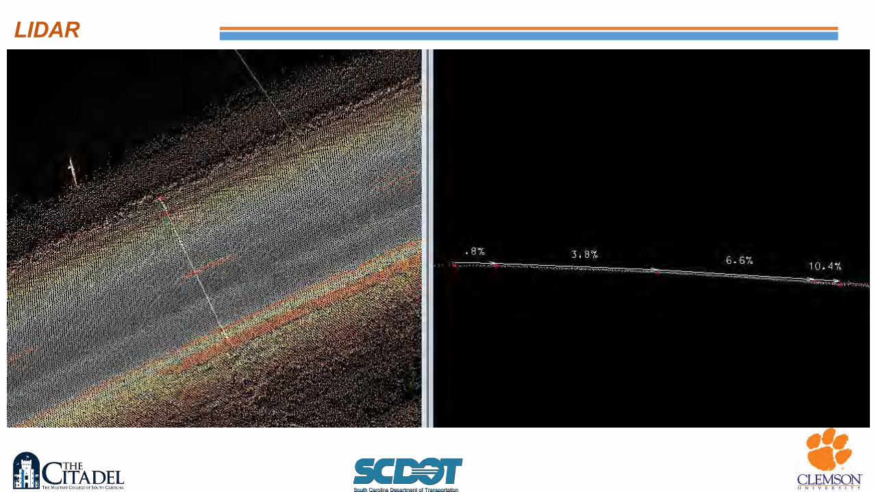
US 123
Ross Ave
LIDAR
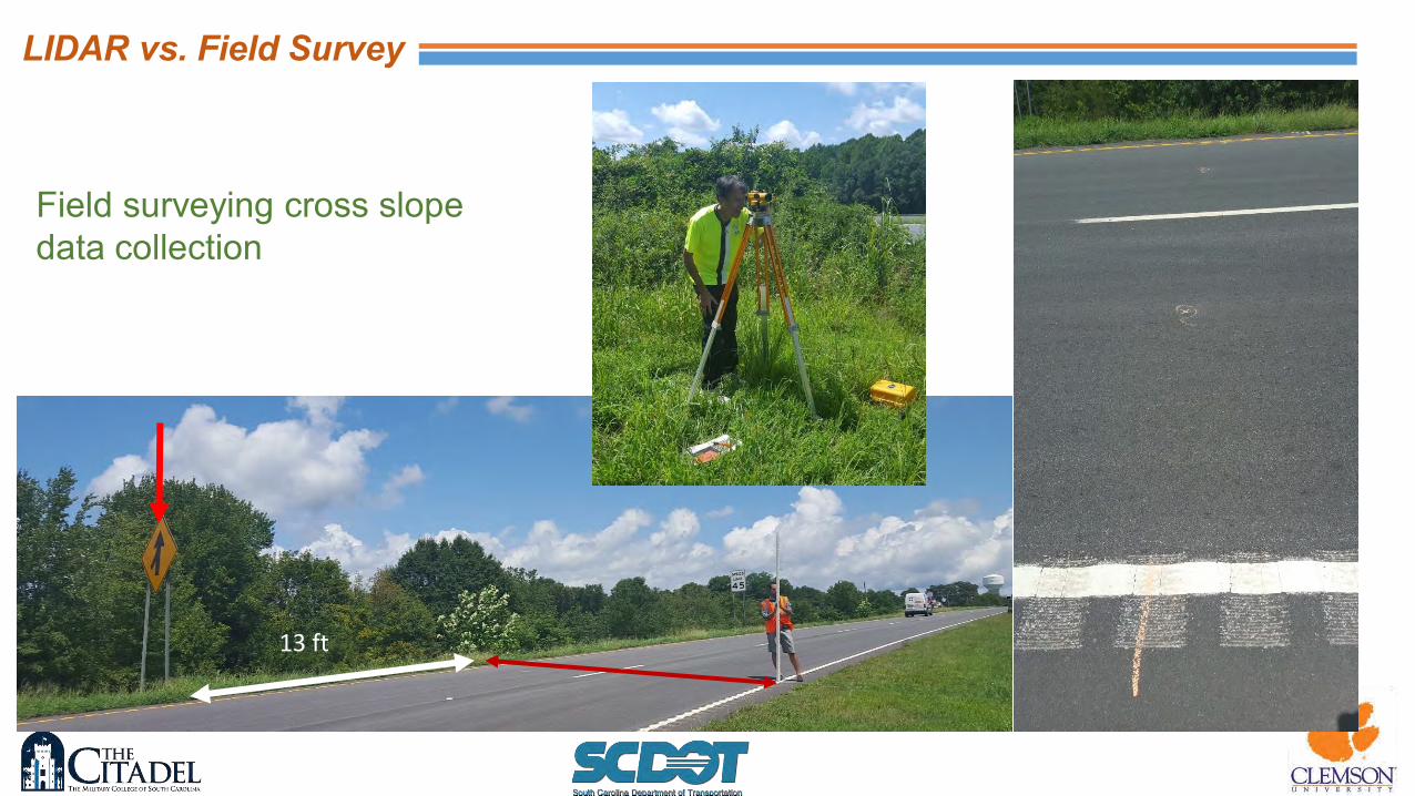
LIDAR vs. Field Survey
13 ft
Field surveying cross slope data collection
LIDAR vs. Field Survey

US 123
Ross Ave
LIDAR
C A B D E F G

Point ID BS Height of Instrument
FS Height (Vertical Distance)
BM 6.55 100
A 106.55 2.03 104.52
B 106.55 2.08 104.47
C 106.55 2.30 104.25
D 106.55 2.55 104.00
E 106.55 2.93 103.62
F 106.55 3.36 103.19
G 106.55 3.55 103.00
Slope Distance
Horizontal Distance
Grade Grade
- - -
2 2 -2.5%
6 6 -3.67% -3.92%
6 5.99 -4.17%
6 5.99 -6.34% -6.77%
6 5.98 -7.19%
2.5
2.49 -7.63%
LIDAR vs. Field Survey
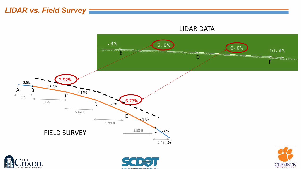
B
2.5%
C
3.67%
D
F
E
4.17%
6.3%
7.6%
7.17%
G
A
6.77%
3.92%
B D
F
LIDAR DATA
FIELD SURVEY
LIDAR vs. Field Survey
2 ft
6 ft
5.99 ft
5.99 ft
5.98 ft
2.49 ft

LIDAR vs. Field Survey

Clemson - Easely
Sign 1 - Guide Sign - Station 34+31
TAPE ROD HEIGHT SLOPE (6 FT) SLOPE(12FT)
SIGN sign 0 8.02 100 -11.18
-11.18
SHOULDER A 34 4.22 103.8 0.50
RIGHT SIDE B 36 4.23 103.79 1.17 1.50
MIDDLE C 42 4.3 103.72 1.83
CENTERLINE D 48 4.41 103.61 0.67
MIDDLE E 54 4.45 103.57 3.17 1.92
LEFT SIDE F 60 4.64 103.38 3.00
SHOULDER G 62 4.7 103.32 9.80 9.80
H 72 5.68 102.34
Field Survey
-3.0% -3.17% -0.67% 1.83% 1.17% 0.5%
CL
-1.92%
1.5%
LIDAR
CL
-2.08% 1.3%
LIDAR
HEIGHT SLOPE(12FT)
RIGHT SIDE 971.82 1.3
CENTERLINE 971.67
2.08 LEFT SIDE 971.42
LIDAR vs. Field Survey
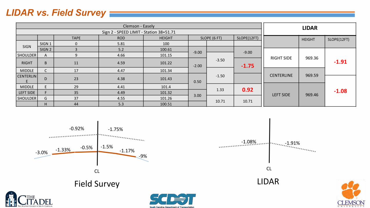
Clemson - Easely
Sign 2 - SPEED LIMIT - Station 38+51.71 TAPE ROD HEIGHT SLOPE (6 FT) SLOPE(12FT)
SIGN SIGN 1 0 5.81 100
SIGN 2 3 5.2 100.61 -9.00
-9.00
SHOULDER A 9 4.66 101.15 -3.50
RIGHT B 11 4.59 101.22 -2.00 -1.75
MIDDLE C 17 4.47 101.34 -1.50 CENTERLIN
E D 23 4.38 101.43
0.50
MIDDLE E 29 4.41 101.4 1.33 0.92
LEFT SIDE F 35 4.49 101.32 3.00
SHOULDER G 37 4.55 101.26 10.71 10.71
H 44 5.3 100.51
Field Survey
-3.0% -1.33% -0.5% -1.5%
-1.17% -9%
CL
-0.92% -1.75%
CL
-1.08% -1.91%
LIDAR
HEIGHT SLOPE(12FT)
RIGHT SIDE 969.36 -1.91
CENTERLINE 969.59
-1.08 LEFT SIDE 969.46
LIDAR
LIDAR vs. Field Survey

Field Survey
-4% -1.5% -0.83% -1.5%
-2.5% -4%
CL
-1.16% -2.0%
Clemson - Easely
Sign 3 - MILE POST - Station 44+19.98 TAPE ROD HEIGHT SLOPE (6 FT) SLOPE(12FT)
SIGN sign 0 5.23 100 -9.00
-9.00
SHOULDER A 5 4.78 100.45 -4.00
RIGHT B 7 4.7 100.53 -2.50 -2.0
MIDDLE C 13 4.55 100.68 -1.5
CENTERLINE D 19 4.46 100.77 0.83
MIDDLE E 25 4.51 100.72 1.50 1.16
LEFT SIDE F 31 4.6 100.63 4.00
SHOULDER G 33 4.68 100.55 10.86 10.86
H 40 5.44 99.79
LIDAR
CL
-1.33% -2.17%
LIDAR
HEIGHT SLOPE(12FT)
RIGHT SIDE 962.17 2.17
CENTERLINE 962.43
1.33 LEFT SIDE 962.27
LIDAR vs. Field Survey

Field Survey
-3% -1.5% -1.0% -1.83%
-2.5% -3%
CL
-1.25% -2.16%
Clemson - Easely
Sign 4 - Guide Sign - Station 44+68.43 TAPE ROD HEIGHT SLOPE (6 FT) SLOPE(12FT)
SIGN sign 0 5.71 100 -10.67
-10.67
SHOULDER I 9 4.75 100.96 -3.00
RIGHT J 11 4.69 101.02 -2.50 -2.16
MIDDLE K 17 4.54 101.17 -1.83
CENTERLINE L 23 4.43 101.28 1.0
MIDDLE M 29 4.49 101.22 1.50 1.25
LEFT SIDE N 35 4.58 101.13 3.00
SHOULDER O 37 4.64 101.07 10.14 10.14
P 44 5.35 100.36
LIDAR
HEIGHT SLOPE(12FT)
RIGHT SIDE 962.20 -2.25
CENTERLINE 962.47
1.42 LEFT SIDE 962.30
LIDAR
CL
-1.42% 2.25%
LIDAR vs. Field Survey
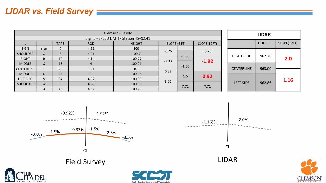
Field Survey
-3.0% -1.5% -0.33% -1.5%
-2.3% -3.5%
CL
-0.92% -1.92%
Clemson - Easely
Sign 5 - SPEED LIMIT - Station 45+92.41 . TAPE ROD HEIGHT SLOPE (6 FT) SLOPE(12FT)
SIGN sign 0 4.91 100 -8.75
-8.75
SHOULDER Q 8 4.21 100.7 -3.50
RIGHT R 10 4.14 100.77 -2.33 -1.92
MIDDLE S 16 4 100.91 -1.50
CENTERLINE T 22 3.91 101 0.33
MIDDLE U 28 3.93 100.98 1.5 0.92
LEFT SIDE V 34 4.02 100.89 3.00
SHOULDER W 36 4.08 100.83 7.71 7.71
X 43 4.62 100.29
LIDAR
HEIGHT SLOPE(12FT)
RIGHT SIDE 962.76 2.0
CENTERLINE 963.00
1.16 LEFT SIDE 962.86
LIDAR
CL
-1.16% -2.0%
LIDAR vs. Field Survey

Field Survey
Clemson - Easely
Sign 6A - GUIDE SIGN - Station 57+39.43 TAPE ROD HEIGHT SLOPE (6 FT) SLOPE(12FT)
SIGN SIGN 1 0 8.45 100
SIGN 2 2.2 7.92 100.53 -10.43
-10.43
SHOULDER A 4.5 7.68 100.77 -9.00
RIGHT B 6.5 7.5 100.95 -8.17 -8.08
MIDDLE C 12.5 7.01 101.44 -8.00
CENTERLINE D 18.5 6.53 101.92 -6.67
MIDDLE E 24.5 6.13 102.32 -6.50 -6.58
LEFT SIDE F 30.5 5.74 102.71 -4.50
SHOULDER G 32.5 5.65 102.8 1.86 1.86
H 39.5 5.78 102.67
CL
4.5% 6.5%
8.0%
-8.2%
-10.4%
-9.0%
6.58%
-8.08%
LIDAR
HEIGHT SLOPE(12FT)
RIGHT SIDE 971.59 -8.08
CENTERLINE 972.56
6.4 LEFT SIDE 973.33
LIDAR
CL
6.41%
-8.08%
LIDAR vs. Field Survey
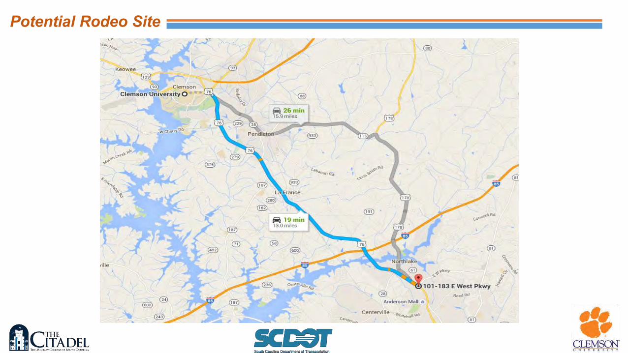
Potential Rodeo Site

Clemson University
Anderson
East West Pkwy

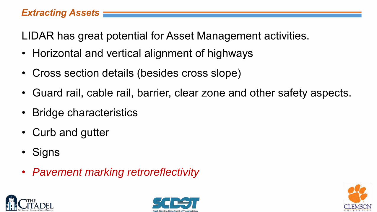
LIDAR has great potential for Asset Management activities. • Horizontal and vertical alignment of highways
• Cross section details (besides cross slope)
• Guard rail, cable rail, barrier, clear zone and other safety aspects.
• Bridge characteristics
• Curb and gutter
• Signs
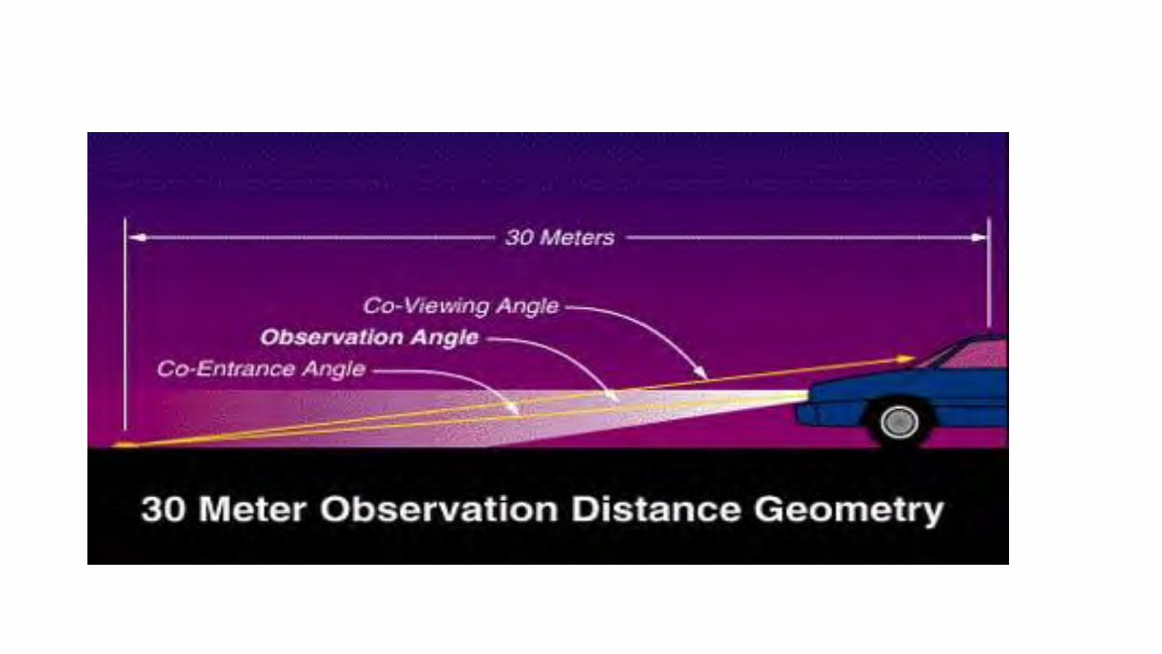
• Pavement marking retroreflectivity
Extracting Assets
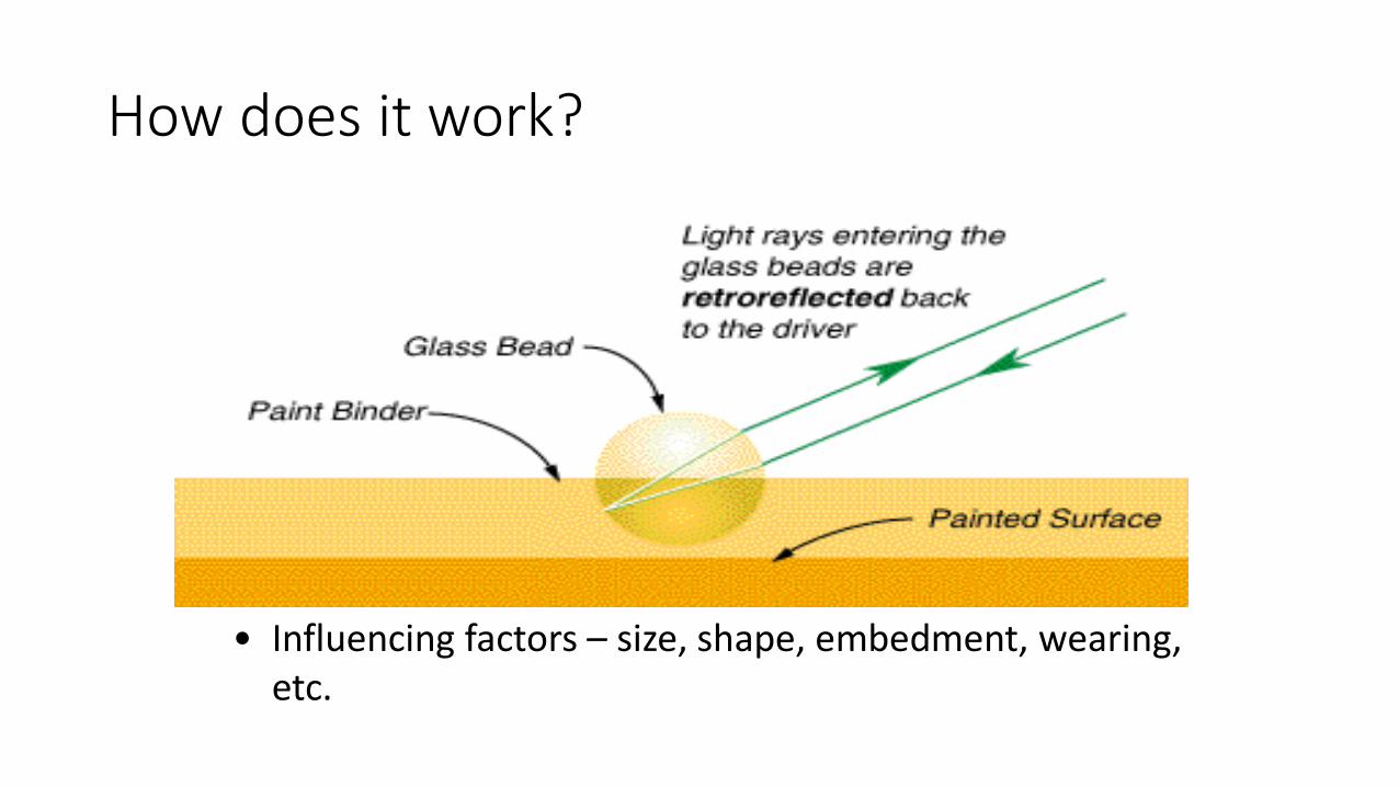
How does it work?
• Influencing factors – size, shape, embedment, wearing, etc.

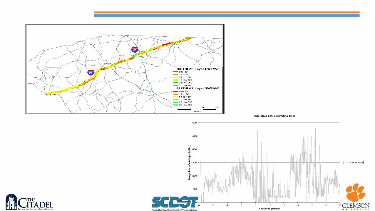
Interstate 526 East White Skip
0
100
200
300
400
500
600
0 2 4 6 8 10 12 14 16 18 20
Distance (miles)
Ave
rage
Ret
rore
flect
ivity
(mcd
/m2/
lux)
Laser data

LIDAR has great potential Is it too much of a good thing? • Processing point clouds is tedious and time consuming
• Intensity/amplitude attribute information is critical for extracting
useful information in an efficient (and possibly automated manner
• Breaklines are needed for preconstruction and major rehab
projects
Final Comments
Thank you