Cross-sectional properties of complex composite beams · PDF fileCross-sectional properties of...

Engineering Structures 29 (2007) 195–212www.elsevier.com/locate/engstruct

Cross-sectional properties of complex composite beams

Airil Y. Mohd Yassina, David A. Nethercotb,∗

a Faculty of Civil Engineering, Universiti Teknologi Malaysia Johor Bahru, Malaysiab Department of Civil and Environmental Engineering, Imperial College, London, United Kingdom

Received 22 September 2005; received in revised form 15 March 2006; accepted 25 April 2006Available online 30 June 2006

Abstract

A procedure is presented for the calculation of the key cross-sectional properties of steel–concrete composite beams of complex cross-section. The novel feature of the procedure is the use of functions to describe the shape of the different elements in a cross-section; this permitsdetermination of the cross-sectional properties through appropriate integrations. The formulation is developed in a format that is directly suitablefor computer programming, i.e. in matrix forms and operations. It is completely general in terms of the shape of the cross-section. The procedureis applied to a new type of composite beam known as the PCFC (pre-cast cold-formed composite) beam, details of which are explained herein.This is shown to perform better than equivalent, more conventional composite beams at the ultimate condition, but is slightly less efficient whenconsidering some serviceability aspects.c© 2006 Elsevier Ltd. All rights reserved.

Keywords: Beams; Composite construction; Flexure; Section properties; Structural design

1. Introduction

The earliest known form of steel–concrete composite beam,dating from the late 1800s, comprised a steel beam encasedin concrete, as shown in Fig. 1(a). The arrangement was firstused in a bridge in Iowa and a building in Pittsburgh [10].The encasement provides fire protection but also enhances thebending strength of the steel beam. Since ultimate strengthdesign was not known at the time, the basis was an elasticassessment. However, with the introduction of ultimate strengthdesign, the eccentricity between the resultant force in theconcrete and that in the steel was recognized as the keyfactor in determining the effectiveness of the composite action.Intuitively, a steel beam located beneath the concrete elementwould result in greater eccentricity and would thus performbetter than the encased section. Such a configuration is shownin Fig. 1(b) in the form of a steel beam connected to theconcrete slab by means of shear connectors [3]. As a way offurther increasing the lever arm, the steel beam can be made

∗ Corresponding address: Imperial College of Science, Technology andMedicine, Department of Civil and Environmental Engineering, London SW72BU, United Kingdom. Tel.: +44 20 7594 6097; fax: +44 20 7594 6049.

E-mail address: [email protected] (D.A. Nethercot).

0141-0296/$ - see front matter c© 2006 Elsevier Ltd. All rights reserved.doi:10.1016/j.engstruct.2006.04.010

asymmetric about its major axis, either by increasing the depthor the width (or both) of the lower flange, as shown in Fig. 1(c)and (d) [2]. Moreover, a reinforced concrete beam, shown asFig. 1(e), can also be loosely regarded as a composite beam butexcluded if the definition requires that the steel element shouldhave substantial flexural stiffness when acting alone, somethingthat the rebar clearly does not possess.

The availability of thin cold-formed steel components in theconstruction industry has led to a new composite configuration,consisting of a steel beam and a composite slab, as shown inFig. 1(f) [4]. New considerations arise for such a configurationas the slab is no longer solid but profiled, thereby influencingthe location of the point of action of the concrete resultant force,the total steel resultant forces (as now there are two sources:the steel beam and the profiled sheeting) and the behaviour ofthe shear connection. Recently, other new slab systems havealso been introduced into composite design such as hollow-cored slabs [6] and pre-cast slabs with a concrete topping [5],as shown in Fig. 1(g) and (h); these lead to new considerations.

Providing the maximum lever arm results in exposure ofthe steel element to compressive forces which may induce localbuckling of the steel (although the possibility is always greaterwhen the steel is acting alone), something that is avoidedwhen using the encased steel beam. To provide both a large

http://www.elsevier.com/locate/engstruct

mailto:[email protected]

http://dx.doi.org/10.1016/j.engstruct.2006.04.010

196 A.Y. Mohd Yassin, D.A. Nethercot / Engineering Structures 29 (2007) 195–212

(a) Encasedsteel section[10].

(b) Composite beamwith solid slab [3].

(c) Cover-platedbeam [2].

(d) Built-up section. (e)Reinforcedconcretebeam.

(f) Composite beamwith compositeslab [4].

(g) Composite beamwith hollow-coreslab [6].

(h) Composite beamwith pre-case slab andconcrete topping [5].

(i) Slim floor [7].

(j)Profiledcompositebeam [11–14].

Fig. 1. Steel–concrete composite cross-sections.

eccentricity and protection against local buckling, a slim-floorsystem was introduced, comprising a steel beam encased eitherfully or partly within the slab. Such a configuration, whichis shown in Fig. 1(i), allows greater concrete width and theprovision of an asymmetric beam compared to the conventionalencased beam of Fig. 1(a) [7].

The use of cold-formed steel is attractive, as it can providepermanent form-work and integral shuttering to the concretesection. In addition to the profiled composite slab, cold-formedsheeting has been used to form the profiled composite beam,as shown in Fig. 1( j), which can be considered as one of themost recent developments in steel–concrete composite beamconstruction [11–14].

1.1. Design consideration of a steel–concrete composite beam

In common with the design of any structural member, asteel–concrete composite beam must be designed to satisfy bothserviceability and ultimate requirements. For the former, designchecks are made against deflection and vibration etc. The mostimportant elastic property of the composite cross-section is itssecond moment of area, which requires transformation of thecross-section into a single unit so as to allow both elements,concrete and steel, to have a similar elastic response. Based onthe full interaction assumption, this is done by multiplying ordividing the area of one of the elements by the modular ratio,

(a) Rectangular stress block for an encased steel section.

(b) Rectangular stress block for a conventional composite beam.

Fig. 2. Rectangular stress block distribution for composite beams.

αe, which is the ratio between the base element’s modulus ofelasticity, Eb, and the modulus of elasticity of the other element,Ee. The calculation must also consider whether the concrete iscracked or uncracked.

When satisfying the ultimate strength requirements, severalaspects of behaviour require checking. Herein, only the ultimatemoment capacity is considered. When determining this, therectangular stress block method is usually adopted. In thisapproach, an element is assumed to be either fully stressed orunstressed. Cross-sectional equilibrium is established betweenthe steel, concrete, reinforcement and shear connectionresultants (if appropriate), and consideration is given to thelocation of the plastic neutral axis, location of the points ofaction of the resultant forces, and the magnitude of the leverarms. The resultant force in each element is taken as theproduct of the material strength and the relevant area; it isassumed to act at the centroid of the stress block. The ultimatemoment capacity is then obtained as the summation of the firstmoment of these resultants about any reference point or level.Fig. 2 shows the ultimate condition and the stress blocks foran encased steel section and a composite beam with a solidslab for the full shear connection condition. Rc and Rs denotethe concrete and steel resultant forces, and subscripts ten andcom refer to tension and compression, respectively. PNA meansplastic neutral axis. There are several possible locations for thePNA: either above the steel section or in the steel upper flangeor in the steel web. If the PNA lies above the steel section, bothcross-sections will have similar stress profiles but, of course,with different magnitudes. However, if the PNA falls within thesteel section then, for the encased steel section, overlappingof the stress profiles occurs. Such an overlap indicates thatthe PNA crosses both the steel and the concrete element, andcomplicates the determination of the location of the PNA.

1.2. PCFC beam

Currently, the authors are developing a new type ofcomposite beam known as a Pre-cast Cold-formed Composite

A.Y. Mohd Yassin, D.A. Nethercot / Engineering Structures 29 (2007) 195–212 197

Fig. 3. Cross-section of PCFC beam.

Beam, or PCFC beam. The beam consists of a closed cold-formed steel section encased in reinforced concrete. A possiblecross-section is illustrated in Fig. 3. Such a configuration canbe considered as a further evolution of the profiled compositebeam shown in Fig. 1( j) for which the additional benefits are:

(i) The cold-formed sheeting provides a hollow core forthe beam and is no longer located at the perimeter ofthe concrete section; therefore, the eccentricity betweenresultants can be adjusted without affecting the beam’souter section.

(ii) Since the cold-formed steel contains no concrete, it doesnot have to be present throughout the depth of the beam,thus reducing the exposure of the steel to compressivestresses. Also, the rigid medium provided by the concreteallows only one-way buckling, a benefit also shared by theprofiled composite beam.

(iii) The encasement eliminates any bearing problem of thecold-formed steel due to the introduction of the load.

(iv) The hollow core can act as a service duct.

The arbitrary shape of the steel section is chosen deliberatelyto emphasize the freedom in geometry that is available whenusing cold-formed steel sections. From the composite beampoint of view, this freedom allows for optimization by matchingthe supply and demand based on the composite beam concept.The extended steel elements are not only part of the steelelement but also act as ‘L-rib’ connectors, making externalshear connectors unnecessary. Although PCFC beams may notexhibit the advantage of providing the permanent formwork ofa profiled composite beam, the prefabricated nature of the beammay be retained by using pre-cast concrete.

Obviously, the PCFC beam also resembles the encased steelbeam and the slim floor type of composite beam. Besides thevoid, the PCFC beam differs from the other two by the use of acold-formed section instead of a hot-rolled or built-up section.Cold-formed sections provide more options in terms of shape.Also, since the cold-formed section is relatively thin, then the‘over-reinforced’ condition, if not desired, can be more easilyavoided.

At the other extreme, the PCFC beam can be consideredas evolving from a conventional reinforced concrete beam. In

Fig. 4. Sources of evolution of the PCFC beam.

this, the role of the concrete in tension is essentially to holdthe reinforcement in place. The cold-formed steel section in aPCFC beam replaces the reinforcement bars of the conventionalreinforced concrete beam, but the void that is created reducesthe amount of concrete in tension.

The evolution of the PCFC beam from its four sources isshown in Fig. 4. However, based on Fig. 3, it is to be expectedthat the design of a PCFC beam will be more complex than isthe case for most of the beams shown in Fig. 1.

The first complication arises from the absence ofrectangularity for the cross-section. The void, the corners andthe irregular steel shape are the cause of this irregularity.Also, the stretching of the sheeting during the formingprocess creates nonuniform thicknesses between corners andflat regions. The immediate effects of these are difficulties indetermining the action point of the force resultants for thevarious components and in transforming the components intoa single unit (required to evaluate the cross-sectional propertiesused for the serviceability checks).

The hybrid properties of cold-formed steel are the nextcomplication. To incorporate the higher strength at the cornersin design, these elements need to be treated individually,increasing the scope of the problem. The simple assumption ofaverage values, on the other hand, reduces the effectiveness ofthe cold-formed steel.

The third complication is due to overlapping between thesteel and concrete elements except in the upper part of thebeam. If the plastic neutral axis locations intersect both the steeland concrete elements, the determination of the location of theplastic neutral axis requires an iteration process. Partial shearconnection introduces a further complication.

1.3. Objectives of the paper

Based on the foregoing discussion, the objectives of thispaper are:

(i) to develop a general procedure for the determination of thecross-sectional properties of complex beam cross-sections,such as the PCFC beam, that is systematic and suitable forcomputer-aided calculation;


(ii) to use this procedure to compare the flexural performanceof the proposed PCFC beam with that of a similar profiledcomposite beam.

2. Design basis of PCFC beam

The key feature of the procedure is the use of functionsto describe the shape of the elements in a cross-section(definitions of elements and function are given in Sections 3.3and 3.4), leading to the determination of the cross-sectional properties through appropriate integrations. This ispresented symbolically, since it is intended for computer-aidedcalculation. Such a procedure has the following advantages:

(i) A systematic procedure reduces calculation and thusreduces the possibility of clumsy errors.

(ii) A computerized procedure provides the basis for a rapiddesign when passing through the various design checks.

(iii) A procedure that is both systematic and computerizedencourages a comprehensive analysis without the need tosimplify the problem (as was inevitably the case for thedesign of profiled composite slabs and profiled compositebeams when using existing approaches).

(iv) The proposed procedure is suitable for mass-productionmanufacturers where products are materially similar butdifferent in scale and shape.

The design basis for the PCFC beam described herein (butwhich is also sufficiently general for use on other complex beamcross-sections) is developed for a beam in positive bending.It covers the determination of the second moment of area ofthe cross-section, assuming full interaction and the ultimatemoment capacity of the beam for both full and partial shearconnection conditions.

2.1. Physical and application stages

The procedure is presented in two stages: the physicalstage and the application stage. The physical stage deals withthe identification of the physical components of the cross-section, their definitions, and their subsequent representationby symbolic expressions. The physical stage provides theunderstanding, including identifying the required data and howto input them. It provides guidance on exactly how to breakdown the complex cross-section into discrete entities whichlater can be prescribed in matrix form. The application stagerepresents these with standard mathematical formulations,arranged to suit computer programming; this stage is intendedfor the implementation. Thus the concepts developed in thephysical stage underpin the mathematical formulations of theapplication stage. A detailed discussion of both stages is givenin Sections 3 and 4 of this paper.

2.2. Design assumptions

The procedure is based on the assumption that beam designis governed by flexure, thus shear-related failures are notconsidered. Also, it is assumed that local buckling does notoccur in the steel elements. The latter assumption holds true

in most cases because of the enhancements provided by theconfiguration of the cross-section, i.e. only one-way localbuckling is possible, and the location of the neutral axis is mostlikely to be relatively high, leaving only a small amount ofsteel in compression. Should the neutral axis lie above the steelsection, then there will be no possibility for local buckling.

The procedure is also based on the assumptions inherent instandard composite beam design, listed as follows:

(i) Steel elements are assumed to be fully stressed to theirdesign strength, py , in both tension and compression, andconcrete elements are assumed to be stressed to a uniformcompressive stress of 0.85 fc throughout the compressiondepth.

(ii) Concrete in tension has negligible strength and is thusneglected.

(iii) Slip is insignificant (full interaction assumption).(iv) Plane sections remain plane.

2.3. Approximation error

Approximation errors will occur if the chosen function doesnot describe the shape of an element exactly. Suitable functionsare proposed in Section 3.4.

3. Physical stage

This stage is concerned with the identification of the physicalcomponents of the cross-section, their definition and symbolicexpression; it has the following components:

(i) symmetricality;(ii) strips;

(iii) elements;(iv) functions;(v) geometrical points.

3.1. Symmetricality

Since the great majority of composite beam cross-sections,especially the forms for which this process has beendevised, are symmetrical about their minor axis, the followingdevelopment is based on this assumption. It permits significantsimplifications to be made.

3.2. Strips

The cross-section is first discretized into a total of Srectangular strips, as shown in Fig. 5. Individual strips arenumbered from 1–S, with a typical strip being referred to asstrip s. Each strip may contain a mix of:

(i) line elements;(ii) bar elements;

(iii) area elements.

Each of these is then represented by a 1-rule continuousfunction, as explained in Section 3.4. The different types ofelements are described below.

3.3. Elements

An area element, a typical example of which is identifiedin Fig. 5, is defined as having significant dimensions in both


Fig. 5. Discretization of a cross-section into S strips.

directions. In comparison, a line element, an example of whichis shown in Fig. 5, is defined as having insignificant dimensionsin one direction compared to the other. Bar elements havenegligible size, are assigned only axial properties, and are usedto represent reinforcement. Thus, in general, area elements areused to represent thick materials such as concrete, while lineelements are employed to represent thin materials such as thinplate, steel sheeting or composite fibres.

Elements are also regarded as either active or passive. Activeelements contribute to the stiffness and strength of the cross-section, while passive elements do not. Thus a void, which isconsidered as an area element, is prescribed as passive. A lineelement representing a boundary is also described as passive,since it does not contribute to either the stiffness or the strengthof the cross-section.

The process of defining and numbering elements within astrip may best be appreciated by referring to a specific example.Consider strip s + 1 of Fig. 5. This contains area elements e1and e3 prescribed as passive since they are voids, area elementse2 and e4 prescribed as active since they consist of concrete,line elements e5 and e9 prescribed as passive since they forminternal and external boundaries of the strip, and line elementse6, e7 and e8 prescribed as active since they represent steelsheeting. Strip s contains a mix of active and passive areaelements, active and passive line elements and the bar elemente10, representing a reinforcing bar.

It is also important to observe certain rules when decidingon the numbering system for elements. This should follow thesequence area elements, followed by line elements, followedby bar elements. It also necessary to preserve the same groupof numbers for the same class of element, i.e. to identify themaximum number of area elements within any one strip, toensure that all area elements in other strips are numberedfrom this group and that line elements and bar elements arenumbered from other groups. Referring again to Fig. 5, it isclear that strip s + 1 contains the largest number of areaelements and line elements. Since any area element must becontained within two line elements, if there are f area elementswithin a strip, then it follows that there must also be f + 1 lineelements within that same strip. Thus the value of f obtainedfrom the strip with the largest number of elements becomes thegoverning factor for subscript numbering for the whole cross-section. Area elements are then referred to as ee≤ f and lineelements are referred to as ee> f , where e = 1, 2, 3, . . . and,for any line element, it is understood that the subscript e cannotbe greater than 2 f + 1. Since bar elements are numbered last,and adopting the subscript g for this class, their range can bestated as 2 f + 1 < g ≤ G, in which G is the total number ofelements existing in that particular strip.

Referring once again to strip s +1 in Fig. 5, which is alreadyidentified as the strip having the largest number of area andline elements, the value of f (and thus f for the whole cross-section) is 4. Thus area elements are denoted as e1–e4 andline elements as e5–e9, with elements closest to the axis ofsymmetry being numbered first. Once this has been recognized,an arbitrary value may be decided for G, providing that it issufficiently large to accommodate all the previously identifiedarea elements and line elements within the most populated stripand then leaves some space for a reasonable presence of barelements within other strips. Referring to strip s of Fig. 5, ithas only two area elements and three line elements. Thus theformer are designated e1 and e2 (with e3 and e4 unused), theline elements are designated as e5–e7 (with e8 and e9 unused),and the single bar element is set as e10 (with e11 set to 0).Continuation of this process for the whole cross-section allowsit to be represented by a matrix of S by G components. For theexample of Fig. 5, S = 8 and G has been chosen as 11, leadingto the matrix representation of Fig. 6. Any element within thismatrix is designated as es,e, where subscripts s and e, whichrepresent the row and column number of the matrix, refer to thenumbering of the strips and elements, respectively.

Fig. 6. The matrix representation of element notation in a cross-section (given in Fig. 5).


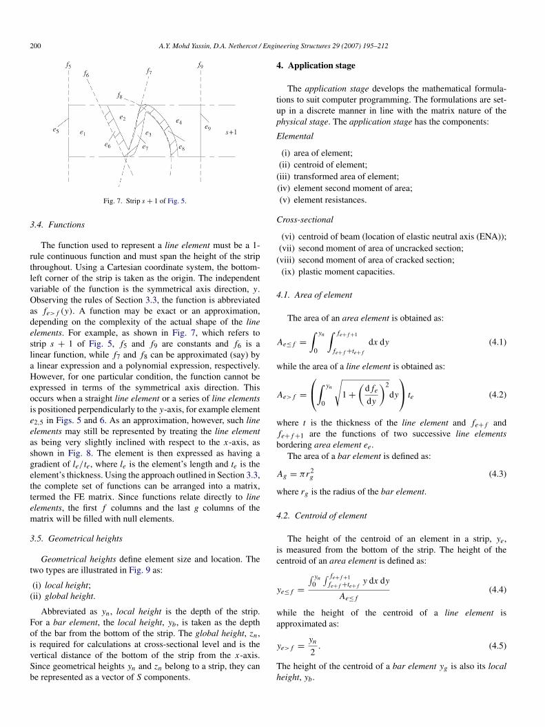
Fig. 7. Strip s + 1 of Fig. 5.

3.4. Functions

The function used to represent a line element must be a 1-rule continuous function and must span the height of the stripthroughout. Using a Cartesian coordinate system, the bottom-left corner of the strip is taken as the origin. The independentvariable of the function is the symmetrical axis direction, y.Observing the rules of Section 3.3, the function is abbreviatedas fe> f (y). A function may be exact or an approximation,depending on the complexity of the actual shape of the lineelements. For example, as shown in Fig. 7, which refers tostrip s + 1 of Fig. 5, f5 and f9 are constants and f6 is alinear function, while f7 and f8 can be approximated (say) bya linear expression and a polynomial expression, respectively.However, for one particular condition, the function cannot beexpressed in terms of the symmetrical axis direction. Thisoccurs when a straight line element or a series of line elementsis positioned perpendicularly to the y-axis, for example elemente2,5 in Figs. 5 and 6. As an approximation, however, such lineelements may still be represented by treating the line elementas being very slightly inclined with respect to the x-axis, asshown in Fig. 8. The element is then expressed as having agradient of le/te, where le is the element’s length and te is theelement’s thickness. Using the approach outlined in Section 3.3,the complete set of functions can be arranged into a matrix,termed the FE matrix. Since functions relate directly to lineelements, the first f columns and the last g columns of thematrix will be filled with null elements.

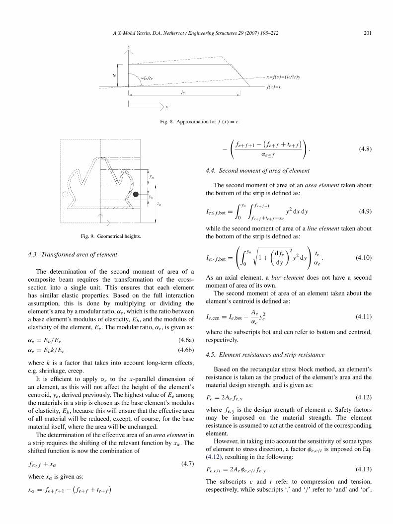
3.5. Geometrical heights

Geometrical heights define element size and location. Thetwo types are illustrated in Fig. 9 as:

(i) local height;(ii) global height.

Abbreviated as yn , local height is the depth of the strip.For a bar element, the local height, yb, is taken as the depthof the bar from the bottom of the strip. The global height, zn ,is required for calculations at cross-sectional level and is thevertical distance of the bottom of the strip from the x-axis.Since geometrical heights yn and zn belong to a strip, they canbe represented as a vector of S components.

4. Application stage

The application stage develops the mathematical formula-tions to suit computer programming. The formulations are set-up in a discrete manner in line with the matrix nature of thephysical stage. The application stage has the components:

Elemental

(i) area of element;(ii) centroid of element;

(iii) transformed area of element;(iv) element second moment of area;(v) element resistances.

Cross-sectional

(vi) centroid of beam (location of elastic neutral axis (ENA));(vii) second moment of area of uncracked section;

(viii) second moment of area of cracked section;(ix) plastic moment capacities.

4.1. Area of element

The area of an area element is obtained as:

Ae≤ f =

∫ yn

0

∫ fe+ f +1

fe+ f +te+ f

dx dy (4.1)

while the area of a line element is obtained as:

Ae> f =

∫ yn

0

√1 +

(d fe

dy

)2

dy

te (4.2)

where t is the thickness of the line element and fe+ f andfe+ f +1 are the functions of two successive line elementsbordering area element ee.

The area of a bar element is defined as:

Ag = πr2g (4.3)

where rg is the radius of the bar element.

4.2. Centroid of element

The height of the centroid of an element in a strip, ye,is measured from the bottom of the strip. The height of thecentroid of an area element is defined as:

ye≤ f =

∫ yn0

∫ fe+ f +1fe+ f +te+ f

y dx dy

Ae≤ f(4.4)

while the height of the centroid of a line element isapproximated as:

ye> f =yn

2. (4.5)

The height of the centroid of a bar element yg is also its localheight, yb.


Fig. 8. Approximation for f (x) = c.

Fig. 9. Geometrical heights.

4.3. Transformed area of element

The determination of the second moment of area of acomposite beam requires the transformation of the cross-section into a single unit. This ensures that each elementhas similar elastic properties. Based on the full interactionassumption, this is done by multiplying or dividing theelement’s area by a modular ratio, αe, which is the ratio betweena base element’s modulus of elasticity, Eb, and the modulus ofelasticity of the element, Ee. The modular ratio, αe, is given as:

αe = Eb/Ee (4.6a)

αe = Ebk/Ee (4.6b)

where k is a factor that takes into account long-term effects,e.g. shrinkage, creep.

It is efficient to apply αe to the x-parallel dimension ofan element, as this will not affect the height of the element’scentroid, ye, derived previously. The highest value of Ee amongthe materials in a strip is chosen as the base element’s modulusof elasticity, Eb, because this will ensure that the effective areaof all material will be reduced, except, of course, for the basematerial itself, where the area will be unchanged.

The determination of the effective area of an area element ina strip requires the shifting of the relevant function by xα . Theshifted function is now the combination of

fe> f + xα (4.7)

where xα is given as:

xα = fe+ f +1 −(

fe+ f + te+ f)

−

(fe+ f +1 −

(fe+ f + te+ f

)αe≤ f

). (4.8)

4.4. Second moment of area of element

The second moment of area of an area element taken aboutthe bottom of the strip is defined as:

Ie≤ f,bot =

∫ yn

0

∫ fe+ f +1

fe+ f +te+ f +xα

y2 dx dy (4.9)

while the second moment of area of a line element taken aboutthe bottom of the strip is defined as:

Ie> f,bot =

∫ yn

0

√1 +

(d fe

dy

)2

y2 dy

teαe

. (4.10)

As an axial element, a bar element does not have a secondmoment of area of its own.

The second moment of area of an element taken about theelement’s centroid is defined as:

Ie,cen = Ie,bot −Ae

αey2

e (4.11)

where the subscripts bot and cen refer to bottom and centroid,respectively.

4.5. Element resistances and strip resistance

Based on the rectangular stress block method, an element’sresistance is taken as the product of the element’s area and thematerial design strength, and is given as:

Pe = 2Ae fe,y (4.12)

where fe,y is the design strength of element e. Safety factorsmay be imposed on the material strength. The elementresistance is assumed to act at the centroid of the correspondingelement.

However, in taking into account the sensitivity of some typesof element to stress direction, a factor φe,c/t is imposed on Eq.(4.12), resulting in the following:

Pe,c/t = 2Aeφe,c/t fe,y . (4.13)

The subscripts c and t refer to compression and tension,respectively, while subscripts ‘,’ and ‘/’ refer to ‘and’ and ‘or’,


respectively. Such a formulation is intended for materials suchas concrete, for which the strength in tension is neglected.Therefore, for most cases, φe,c can be taken as unity.

Strip resistance is the total of the element resistances withinthe strip. To take into account the sensitivity to stress direction,the strip resistance is again categorized into:

(i) compressive strip resistance, Rc =

∑Pe,c (4.14a)

(ii) tensile strip resistance, Rt =

∑Pe,t . (4.14b)

4.6. Centroid of beam

The determination of the centroid of a cross-section alsolocates the position of the elastic neutral axis since, underthe elastic and full interaction assumption, both points arecoincident.

The centroid of the cross section, Y , measured from the x-axis is defined as:

Y =

S∑s=1

Ae (ye + zn)

S∑s=1

Ae

. (4.15)

4.7. Second moment of area of beam (uncracked section)

The second moment of area of an uncracked section, Ix,un,about the centroid of the beam parallel to the x-axis isdetermined using the Parallel Axes Theorem. This is definedas:

Ix,un = 2∑

Ie,cen +Ae

αed2

e (4.16)

where the subscript ‘un’ refers to uncracked. For an elementhaving its centroid higher than or coincident with the centroidof the cross-section (i.e. ye + zn > Y ),

de = zn − Y + ye. (4.17a)

For an element having its centroid lower than the centroid ofthe cross-section, (i.e. ye + zn < Y )

de = Y − ye − zn . (4.17b)

4.8. Second moment of area of beam (cracked section)

For a cracked concrete section, the elastic neutral axis(ENA) no longer coincides with the centroid of Eq. (4.15). Thedetermination of the location of the ENA can be carried out byequating the first moment of area between the ‘upper’ regionand the ‘lower’ region of the cross-section. This requires aniteration process to locate the strip within which the ENA falls.However, this is thought to be unnecessary, as the exact locationof the ENA will most likely remain close to the centroidand a simplified approach is adopted here. (A full procedureinvolving iteration is devised for the plastic neutral axis (PNA)later.)

Therefore, for the determination of the second moment ofarea of the cracked concrete section, Ix,cr, it is assumed thatthe ENA and the centroid of Eq. (4.15) remain coincident.Ix,cr is thus taken as Ix,un, with the second moment of areaof the concrete in tension subtracted from it. By assuming thatthe centroid of the beam lies in strip q, and if all active areaelements are concrete elements, the second moment of area ofa cracked section, Ix,cr, about the centroid of the beam parallelto the x-axis is obtained as:

Ix,cr = Ix,un − 2

(s=q−1∑

s=1

Ie≤ f,cen +Ae≤ f

αe≤ f(Y − ye − zn)2

)

− 2(

Ie≤ f,cen +Ae≤ f

αe≤ f(Y − ye − zn)2

)q,t

(4.18)

where the subscript ’cr’ refers to cracked. The first bracketcontains concrete terms extracted from strips lower than stripq and the second bracket contains concrete terms in tension forstrip q. All the terms in the first bracket have been calculatedpreviously as Eqs. (4.1) and (4.4). These equations are alsoreused to determine the terms in the second bracket by replacingthe upper integration limit in the y-direction, yn with Y − zn .

4.9. Plastic moment capacities

The plastic moment capacity of a composite beam iscalculated using the rectangular stress block approach. Theultimate condition of the beam is governed by the degreeof shear connection, defined as the ratio of the longitudinalshear strength provided compared to that required for full shearconnection. Herein, the determination of the plastic momentcapacity of the composite beam is explained first for the generalcase of partial shear connection and is then specialized for thetwo extreme cases, i.e. full and zero shear connection.

In a conventional steel–concrete composite beam, partialshear connection occurs when the resultant force from theshear connectors, termed Fb, is smaller than the weaker of theaxial resistance of the concrete section or the steel section,respectively termed Fc and Fs . Fc and Fs are obtained asthe product of the material strength and the whole cross-sectional area of the concrete or the steel. Such easy checkingof the partial shear connection condition is possible becausethe concrete and the steel elements are placed at differentlevels, as shown in Fig. 10(a) for a beam in positive bending.The condition requires that, to obtain the full shear connectioncondition, at least one material must have fully yielded in onedirection. Although there can be two full shear connectionconditions, i.e. PNA in the concrete or in the steel, becauseboth elements must yield in both directions there is a uniquepartial shear connection condition for the beam, as shown inthe figure, and since neither of the elements yields completelyin one direction, there exists two locations for the plastic neutralaxis (PNA).

In a profiled composite beam, on the other hand, theelements are placed largely at the same level, thus making sucha check impossible because, even for the full shear connectioncondition, each element is subjected to both compression and


Fig. 10. Possible equilibrium conditions of composite beams.

acts

tension. The systematic approach for determining the levelof partial shear connection is to first calculate the minimumlongitudinal shear resultant required to achieve full shearconnection, Fb,min, and to compare it with the value of Fb

provided; this step will be illustrated later. But a condition thatalways prevails for the partial condition is that the concreteresultant force, Fc,com, will always be smaller than the valuerequired for full shear connection. In Fig. 10(b), Fc,com isthe resultant force for the smaller white rectangular stressblock. This is an important observation which will be used indetermining the minimum longitudinal shear resultant, Fb,min.

In a PCFC beam, there are two possible locations for thePNA for the full shear connection condition, since the PNA canbe in either the upper part of the concrete section or the steelsection, and there are also two possible partial shear connectionconditions, as shown in Fig. 10(c). Despite the various possibleshapes for the stress block, the force distributions are similarfor all beams, as given in Fig. 11.

4.9.1. Minimum longitudinal shear force for full shearconnection — Fb,min

To determine whether a beam exhibits the partial shearconnection condition, a check can be made against theminimum resultant longitudinal shear force, termed Fb,min

(a) Distribution of forces for full shear connection.

(b) Distribution of forces for partial shear connection.

Fig. 11. Distribution of forces in a composite beam.

nd defined as the minimum value necessary for full shearonnection. If Fb provided is less than the calculated Fb,min,hen partial shear connection exists. This single check isufficient for a profiled composite beam, since there is a unique


full shear connection condition for the beam. For a PCFC beam,however, since Case 2 for full shear connection resembles thecondition of the conventional composite beam, Fb must inaddition be less than the steel axial resistance Fs .

An established approach to determining Fb,min is to equatethe location of the PNA in the concrete section to the locationof the PNA in the steel section. This approach has been outlinedby Oehlers et al. [12]. Their argument is that, since, in thistype of beam, the full shear condition and full interaction arenot distinguishable, at these conditions slip strain must be zeroand hence the PNA in both elements must be coincident. Thisapproach is suitable for their simplified arrangement, sincethere is only one possible location for the PNA, i.e. withinthe depth of the steel web. In the present procedure, sincethere are more possibilities for the location of the PNA dueto the discretization of the cross-section into strips, a differentapproach for the determination of Fb,min is adopted.

Since the plastic moment capacity of a composite beam withpartial shear connection cannot exceed the capacity obtainedfor full shear connection, the latter condition requires thatall elements must have yielded, since the presence of anyunyielded portion of material would imply a possibility for thecapacity to increase. Examining this by referring to Fig. 12,which shows the force distributions in both the concrete sectionand steel section for full and partial shear connection, identifieseight force components as follows:

Fc,full is the concrete section compressive resistance for thefull shear condition;

Fc,com is the concrete section compressive resistance for thepartial shear condition;

Fg,com is the compression resistance of the rebar for both fulland partial shear conditions;

Fg,ten is the tension resistance of the rebar for both full andpartial shear conditions;

Fb,min is the minimum longitudinal shear resultant forcerequired to achieve the full shear connectioncondition;

Fb is the longitudinal shear connection resultant actuallyprovided = τb Sr nr Lwhere τb is the rib shear strength, Sr is the interfaceperimeter (as shown in Fig. 12), nr is the number ofribs in the cross-section, and L is the distance of thecritical cross-section from the support or the point ofcontraflexure.

Fs,com is the steel section compressive resistance for full orpartial shear conditions;

Fs,ten is the steel section tension resistance for full or partialshear conditions.

For both connection conditions, it can seen that Fg,comand Fg,ten have fixed magnitudes, based on the assumptionthat rebar is always fully yielded. Thus, this leaves only twocomponents in the concrete section, Fc,full and Fb,min for thefull shear connection condition and Fc,com and Fb for the partialshear connection condition; any change in the magnitude of onewill affect the other. Since any reduction in Fb from its limitFb,min will reduce Fc,com from its limit Fc,full, Fb,min is thus the

Fig. 12. Shape/perimeter of ribs.

force required for the concrete section to obtain its maximumresultant Fc,full, which in turn depends on the unique concretecrushing depth, i.e. the location of the PNA at the full shearconnection condition. Based on this, Fb,min can be calculated bydetermining first the location of the PNA for this full condition.

The determination of the location of the PNA for the fullshear connection condition requires an iteration process. Asmentioned in Section 1.1, for a conventional composite beam,there are three possible locations for the PNA: in the concretesection, in the upper steel flange or in the steel web. For a PCFCbeam, there are more options, so it is necessary to derive analgorithm to drive the iteration process for locating the stripwithin which the PNA lies. PNA falls in strip p when:

S∑s=S−k+1

(Rc)s >

S−k∑s=1

(Rt )s (4.19)

where p = S − kh + 1 and kh is the kth attempt in which Eq.(4.19) is satisfied.

Based on Eq. (4.19), it can be seen that the determinationfor strip p depends on kh , which is the cycle number of theiteration needed in satisfying Eq. (4.19). The application of Eq.(4.19) is illustrated in Example 2. Once the strip in which thePNA falls has been identified, the exact location of the PNAcan be determined. The height of the PNA measured from thebottom of strip p, h f can be obtained by solving the followingequality:∑i=0

(Rc)p+i+1≤S +

(∑Pe,c

)p,c

=

∑i=0

(Rt )p−i−1≥1

+

(∑Pe,t

)p,t

+

(∑Pg

)p

(4.20)

in which(Pe,c

)s,c and

(Pe,t

)s,t are the partial element

resistances in strip p, being separated by the PNA. Thesepartial values can be determined by the reuse of Eqs. (4.1) and(4.2), substituting the integration limit in the y-direction, yn , byyn − h f and h f for the compressive part and the tensile part,respectively.

Once h f is determined, Fb,min can be determined as follows.Eq. (4.20) actually expresses the internal equilibrium of thewhole cross-section, not distinguishing elements or materials.An individual equilibrium of, say, the concrete section canbe obtained by extracting the terms containing area elementsand bar elements from Eq. (4.20). The residual resultant of


the extracted terms is then balanced by an equal resultantforce in the opposite direction, contributed by the compositeaction. Since this resultant is the force required for the concretesection to maintain its full shear connection equilibrium, thiscountering resultant is therefore the desired Fb,min, which cannow be given as:

Fb,min =

∑i=0

(Pg,t

)p−i−1≥1 +

(∑Pg

)p

−

∑i=0

(Pg,c

)p+i+1≤S −

∑i=0

(Pe≤ f,c

)p+i+1≤S

−

(∑Pe≤ f,c

)p,yp−h f

. (4.21)

Eq. (4.21) states that Fb,min is equal to the residualbetween the compressive forces and the tensile forces inthe concrete section. The fourth term on the right-hand sideof the equation,

(∑Pe≤ f,c

)p,yp−h f

, represents the partialcompressive resistance of strip p. The height of the compressiveregion of strip p is given by the subscripts yp − h f , whereyp is the local height of strip p and h f is the height of thePNA measured from the bottom of strip p, a known value.If the first two terms on the right-hand side of the equationare represented as Fg,ten, the third term as Fg,com and the lasttwo terms as Fc,full, then Eq. (4.21) actually expresses theequilibrium condition of the concrete section of Fig. 11(a).Based on Eq. (4.21), Fb,min, and thus Fb, can be compressive ortensile. Although the direction of Fb,min, (or Fb) in the concretesection would not have any effect on the behaviour of the beam,because it will be equated by a force of equal magnitude actingat the same point but in the opposite direction from the steelsection, the present procedure requires the direction obtainedfrom Eq. (4.21) to be maintained. To note, the direction ofFb,min is also the direction of Fb.

4.9.2. Location of PNA for partial shear connectionIn determining the plastic moment capacity of a composite

beam with partial shear connection, the locations of the plasticneutral axis (PNA) must be determined first. The determinationrequires knowledge of the magnitude and direction of Fb, forwhich a method has been outlined in Section 4.9.1. Once theseare known, the next step is to identify the strip in which the PNAis located. For longitudinal equilibrium in the concrete section,the PNA lies in strip pc when:

S∑s=S−k+1

(Pe≤ f/g,c

)s + Fb >

S−k∑s=1

(Pg,t

)s (4.22)

where pc = S − kc + 1 and kc is the kth attempt in whichEq. (4.22) is satisfied. For longitudinal equilibrium in the steelsection, the PNA lies in strip ps when:

S∑s=S−k+1

(Pe> f,c

)s >

S−k∑s=1

(Pe> f,t

)s + Fb (4.23)

where ps = S − ks + 1 and ks is the kth attempt in which Eq.(4.23) is satisfied.

The exact location of the PNA can then be determinedas follows. The height of the PNA in the concrete sectionmeasured from the lowest local point of strip pc, h pc, can beobtained by solving the following equality:∑i=0

(Pe≤ f/g,c

)pc+i+1≤S +

(∑Pe≤ f,c

)pc,c

+ Fb

=

∑i=0

(Pg,t

)pc−i−1≥1 (4.24)

while the equality for determining the height of the PNA in thesteel section h ps is given as:∑i=0

(Pe> f,c

)ps+i+1≤S +

(∑Pe> f,c

)ps ,c

=

∑i=0

(Pe> f,t

)ps−i−1≥1 +

(∑Pe> f,t

)ps ,t

+ Fb (4.25)

where the partial values can be determined by replacing theintegration limit, yn , with yn − h pc and h pc of the compressivepart and the tensile part of the concrete, respectively, or yn −h psand h ps of the steel part, respectively.

4.9.3. Plastic moment capacity for partial shear connectionOnce h pc and h ps are determined, the individual section

contributions to the plastic moment capacity, Mconc and Msteel,can be determined, as follows:

Mconc =

∑i=0

(Pe≤ f/g,cze≤ f/g

)pc+i+1≤S

+

(∑Pe≤ f,cze≤ f,c

)pc,c

−

∑i=0

(Pg,t zg

)pc−i−1≥1 (4.26)

Msteel =

∑i=0

(Pe> f,cze> f

)ps+i+1≤S

+

(∑Pe> f,cze> f,c

)ps ,c

−

∑i=0

(Pe> f,t ze> f

)ps−i−1≥1

−

(∑Pe> f,t ze> f,t

)ps ,t

(4.27)

in which the zs are the lever arm of an element measured fromthe bottom of the cross-section. These lever arms are given ingeneral terms as follows. To obtain the value for a particulargroup of elements, just add to the subscript e the relevantrange, either ≤ f or > f , and add to the subscript p the relevantsubscript, either c or s:

ze = ye + zn or yb + zn (4.28)

ze,c = ye + h p + zn (4.29)

ze,t = ye + zn (4.30)

zg = yb + zn . (4.31)

Finally, the plastic moment capacity of the composite cross-section for partial shear connection, Mpartial, is given as:

Mpartial = Mconc + Msteel. (4.32)


4.9.4. Note on the existing formulation [12]Flexural strength formulations for a profiled composite beam

of the type shown in Fig. 13(a) have been derived by Oehlerset al. [12] for both the full and the partial shear connectionconditions. The formulations require the cross-section to besimplified into the equivalent form shown in Fig. 13(b).Based on this simplified cross-section, the formulations applyspecifically to a cross-section consisting of a steel trough(formed by two steel webs, which are connected at thebase by a steel flange) that surrounds a rectangular concretecore reinforced in tension. This limitation is apparent in theformulation for the plastic moment capacity for the partial shearconnection, given as follows:

Mpartial = Fpy y − 2te f py (1 + β) N 2p + Fbdb

+

(Fsyde −

12

0.85γ 2 fcwe N 2c − Fbdb

)(4.33)

in which:

Fpy is the resultant force for the whole steel section =

(2De + we)te f py

y defines the point of action of Fpy

De, te, we are simplified geometrical properties shown inFig. 13

f py is the profiled sheeting yield stressNp is the depth of the plastic neutral axis in the steel

section measured from the upper surface of the cross-section

db and de define the points of action of Fb and Fsy ,respectively

Fsy is the resultant force from the tensile reinforcementfc is the concrete compressive strengthNc is the depth of the plastic neutral axis in the concrete

section measured from the upper surface of the cross-section

β is a reduction factor used in considering the effect oflocal buckling (taken in this procedure as unity)

γ is a concrete nonlinearity correction factor (taken inthis procedure as unity).

The limitation due to the required geometrical simplificationis evident from the 2 multiplier, as it represents the two straight-rectangular-vertical webs of the profiled sheeting. Shouldthe number of webs be different from two, or the steelcomponent be irregular in shape, the formulation is no longervalid. Another limitation is also obvious, since there is nocompression reinforcement term in Eq. (4.33). Such limitationsare not present in the new procedure.

4.9.5. Plastic moment capacity of extreme conditionsThe plastic moment capacity of the full shear connection and

zero shear connection conditions can be determined by settingthe value of Fb in each of Eqs. (4.22)–(4.25) equal to Fbmin orto zero, respectively.

(a) Actual cross-section.

(b) Simplified cross-section.

Fig. 13. Analyzed cross-section [13,14] — (Example 3).

5. Worked examples

A program has been written using Matlab7 [8] to implementthe above procedure and has been used to perform calculationsfor the following examples. The basic structure of the programis the conversion of the physical description of the cross-sectioninto a series of matrix operations. This is made possible bythe notation system and the discreteness of the formulationprocedure. For example, the area of the eth area element inthe sth strip is expressed by Eq. (4.1) as (Ae)s . But, if elementnumbering and strip numbering are treated as the columns andthe rows of a matrix AE, the area can equally be expressed asAE(s, e) and so become an element of matrix AE. Readers areencouraged to observe the given Matlab program scripts, whichillustrate exactly how the formulations are put into practice. Inparticular:

(i) Terms expressed in capital letters are complete matrices,i.e. FE, TE, etc.

(ii) Terms where the first letter is a capital refer to incompletematrices, i.e. Ae, Aef, etc. These matrices are incomplete,because they contain the components according to thespecific group of elements, i.e. area, line, bar. They arelater algebraically added to form a complete matrix.

(iii) Terms expressed in lower-case letters refer to a componentof a matrix, i.e. ae, aef, etc.

5.1. Example 1

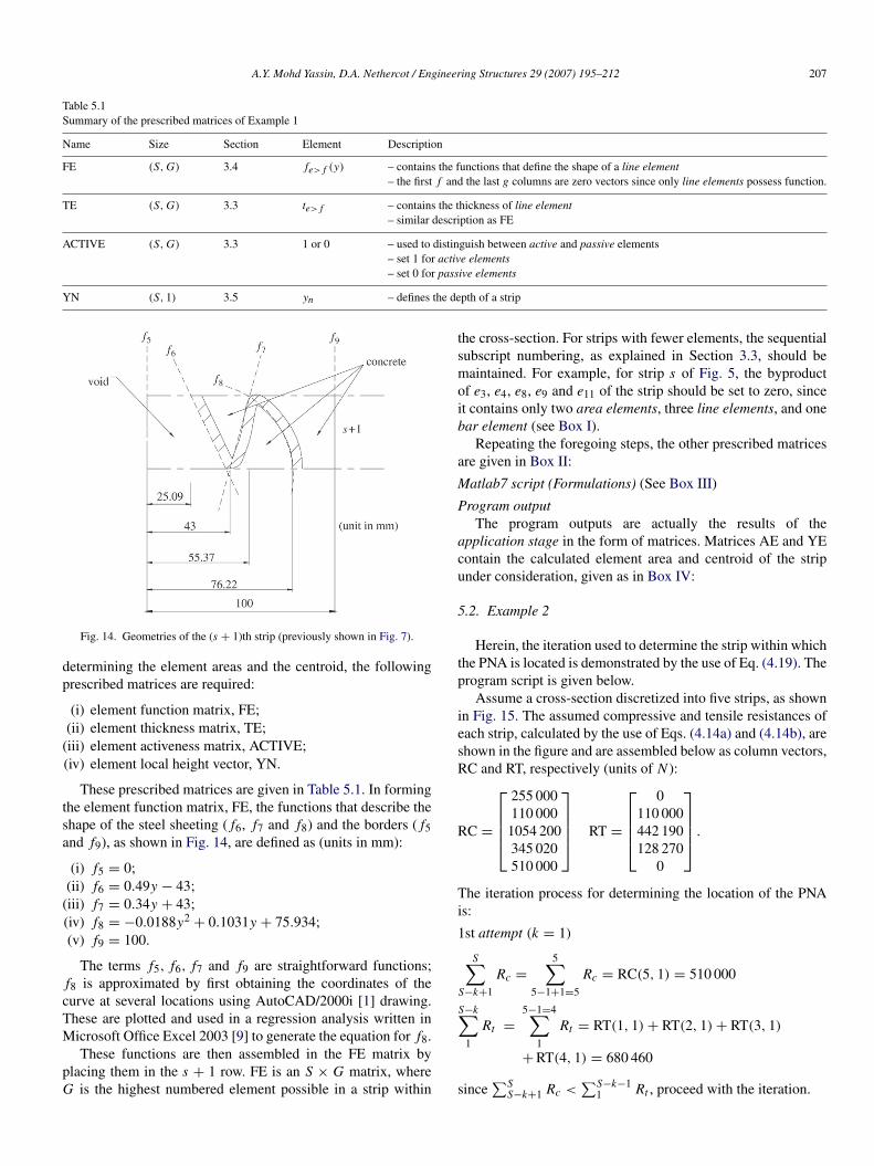
The first example deals with the properties of the singlestrip illustrated in Fig. 14; this is strip s + 1 from Fig. 7. Theinput data for the calculation are prescribed ‘directly’ in matrixform. These input data are obtained from the physical stage. In


Table 5.1Summary of the prescribed matrices of Example 1

Name Size Section Element Description

FE (S, G) 3.4 fe> f (y) – contains the functions that define the shape of a line element– the first f and the last g columns are zero vectors since only line elements possess function.

TE (S, G) 3.3 te> f – contains the thickness of line element– similar description as FE

ACTIVE (S, G) 3.3 1 or 0 – used to distinguish between active and passive elements– set 1 for active elements– set 0 for passive elements

YN (S, 1) 3.5 yn – defines the depth of a strip

dp

(

tsa

(

cTM

pG

Fig. 14. Geometries of the (s + 1)th strip (previously shown in Fig. 7).

etermining the element areas and the centroid, the followingrescribed matrices are required:

(i) element function matrix, FE;(ii) element thickness matrix, TE;iii) element activeness matrix, ACTIVE;

(iv) element local height vector, YN.

These prescribed matrices are given in Table 5.1. In forminghe element function matrix, FE, the functions that describe thehape of the steel sheeting ( f6, f7 and f8) and the borders ( f5nd f9), as shown in Fig. 14, are defined as (units in mm):

(i) f5 = 0;(ii) f6 = 0.49y − 43;iii) f7 = 0.34y + 43;

(iv) f8 = −0.0188y2+ 0.1031y + 75.934;

(v) f9 = 100.

The terms f5, f6, f7 and f9 are straightforward functions;f8 is approximated by first obtaining the coordinates of theurve at several locations using AutoCAD/2000i [1] drawing.hese are plotted and used in a regression analysis written inicrosoft Office Excel 2003 [9] to generate the equation for f8.These functions are then assembled in the FE matrix by

lacing them in the s + 1 row. FE is an S × G matrix, whereis the highest numbered element possible in a strip within

the cross-section. For strips with fewer elements, the sequentialsubscript numbering, as explained in Section 3.3, should bemaintained. For example, for strip s of Fig. 5, the byproductof e3, e4, e8, e9 and e11 of the strip should be set to zero, sinceit contains only two area elements, three line elements, and onebar element (see Box I).

Repeating the foregoing steps, the other prescribed matricesare given in Box II:

Matlab7 script (Formulations) (See Box III)

Program outputThe program outputs are actually the results of the

application stage in the form of matrices. Matrices AE and YEcontain the calculated element area and centroid of the stripunder consideration, given as in Box IV:

5.2. Example 2

Herein, the iteration used to determine the strip within whichthe PNA is located is demonstrated by the use of Eq. (4.19). Theprogram script is given below.

Assume a cross-section discretized into five strips, as shownin Fig. 15. The assumed compressive and tensile resistances ofeach strip, calculated by the use of Eqs. (4.14a) and (4.14b), areshown in the figure and are assembled below as column vectors,RC and RT, respectively (units of N ):

RC =

255 000110 0001054 200345 020510 000

RT =

0

110 000442 190128 270

0

.

The iteration process for determining the location of the PNAis:

1st attempt (k = 1)

S∑S−k+1

Rc =

5∑5−1+1=5

Rc = RC(5, 1) = 510 000

S−k∑1

Rt =

5−1=4∑1

Rt = RT(1, 1) + RT(2, 1) + RT(3, 1)

+ RT(4, 1) = 680 460

since∑S

S−k+1 Rc <∑S−k−1

1 Rt , proceed with the iteration.


FE =

1 2 3 4 5 6 7 8 9 10 111 · · · · · · · · · · ·

· · · · · · · · · · ·

s + 1 0 0 0 0 0 (0.49y − 43) (0.34y + 43) (−0.0188y2+ 0.1031y + 75.934) 100 0 0

· · · · · · · · · · ·

S · · · · · · · · · · ·

f f + 1 g

Box I.

TE =

1 2 3 4 5 6 7 8 9 10 111 · · · · · · · · · · ·

· · · · · · · · · · ·

s + 1 0 0 0 0 0 2 2 2 0 0 0· · · · · · · · · · ·

S · · · · · · · · · · ·

f f + 1 g

ACTIVE =

1 2 3 4 5 6 7 8 9 10 111 · · · · · · · · · · ·

· · · · · · · · · · ·

s + 1 0 1 0 1 0 1 1 1 0 0 0· · · · · · · · · · ·

S · · · · · · · · · · ·

f f + 1 g

YN =

1 ·

·

s + 1 36.69·

S ·

Box II.

Fig. 15. Assumed cross-section resultants (units in N).

2nd attempt (k = 2)

S∑S−k+1

Rc =

5∑5−2+1=4

Rc = RC(4, 1) + RC(5, 1) = 855 020

S−k∑1

Rt =

5−2=3∑1

Rt = RT(1, 1) + RT(2, 1) + RT(3, 1)

= 570 460

since∑S

S−k+1 Rc >∑S−k−1

1 Rt , stop iteration. kh = 2 hencep = S − kh + 1 = 4 (PNA lies in strip 4).

Matlab7 script

for k=1:SkRIGHT=double(sum(RC(S-k+1:S,1)))LEFT=double(sum(RT(1:S-k,1)))if RIGHT>LEFT

breakend

endp=S-k+1

5.3. Example 3 (validation of the procedure)

Application to an actual beam cross-section is demonstratedand validated by analyzing the profiled composite beam cross-section shown in Fig. 1( j). Results are then compared with thoseobtained from the original formulation [12]. This formulationdid not allow for the actual shape of the cross-sectionand required the cross-section be simplified. Compressionreinforcement was not included. The cross-section is the onepreviously studied by Uy and Bradford [13,14] shown inFig. 13. Full shear connection is considered (the values ofFb min are as calculated in Example 5 for a partial shearconnection analysis). It is also assumed that the concrete


Element areaThe following is the program script for the determination of the element area written in Matlab7.

Ae=zeros(S,G)Aef=zeros(S,G)Ag=zeros(S,G)

for e=1:ffor s=1:S

ae=(int(FE(s,e+f+1)-(FE(s,e+f)+TE(s,e+f)),0,YN(s,1))) % - - - - - - - - - Equation (4.1)Ae=[zeros(s-1,G);zeros(1,e-1),ae,zeros(1,G-e); zeros(S-s,G)]+Ae

endendfor e=f+1:2*f+1for s=1:S

aef=(int((1+(diff(FE(s,e))2̂))0̂.5,0,YN(s,1)))*TE(s,e)% - - - - - - - - - - - - - - - - - - - - - Equation (4.2)Aef=[zeros(s-1,G);zeros(1,e-1),aef,zeros(1,G-e);zeros(S-s,G)]+Aef

endendfor e=2*f+2:Gfor s=1:S

ag=pi*(RE(s,(e))) 2% - - - - - - - - - - - - - - - - - - - - - - - - - - - - - - - - - - - - - - - - - - - - - - - - - - - - -Equation (4.3)Ag=[zeros(s-1,G);zeros(1,e-1),ag,zeros(1,G-e);zeros(S-s,G)]+Ag

endendAE=Ae+Aef+Ag

Effective areaAE contains the areas of all elements including the passive elements. To remove these, AE is multiplied, element-by-element (using operator (.∗))by the ACTIVE matrix, as follows:

AE=ACTIVE.*AE

Element centroidThe script for the determination of the element centroid is given below.

Ye=zeros(S,G)Yef=zeros(S,G)Yg=zeros(S,G)

for e=1:ffor s=1:S

ye=((int(FE(s,e+f+1)*y-(FE(s,e+f)+TE(s,e+f))*y,0,YN(s,1)))/AE(s,e)) % - - - - - - - - - Equation (4.4)Ye=[zeros(s-1,G);zeros(1,e-1),ye,zeros(1,(G)-e);zeros(S-s,G)]+Ye

endendfor e=f+1:2*f+1for s=1:S

yef=YN(s,1)/2% - - - - - - - - - - - - - - - - - - - - - Equation (4.5)Yef=[zeros(s-1,G);zeros(1,(e)-1),yef,zeros(1,(G)-(e));zeros(S-s,G)]+Yef

endendfor e=2*f+2:Gfor s=1:S

yg=YB(s,1) % - - - - - - - - - - - - - - - - - - - - - - - - - - - - - - - - - - - - - - - - - - - - - - - - - - - - - - - - - - - - - - - - - - - - - - - - - - - - - - -Equation (4.5)Yg=[zeros(s-1,G);zeros(1,e-1),yg,zeros(1,G-e);zeros(S-s,G)]+Yg

endendYE=Ye+Yef+Yg

Omitting NaN and inf elements

Since AE contains zero elements, YE obtained above contains NaN (not-a-number) and/or inf (infinity) elements; terms used by Matlab7. Theformer occurs when zero is divided by zero, whilst the latter occurs when a number is divided by zero. To omit these elements from YE, thefollowing script is written for the program.

for e=1:Gfor s=1:Sif YE(s,e)== NaN

YE(s,e)=0elseif YE(s,e)== Inf

YE(s,e)=0endendendend

Box III.


AE =

· · · · · · · · · · ·

· · · · · · · · · · ·

s + 1 0 2.981e3 0 1.0497e3 0 81.7 77.5 88.8 0 0 0· · · · · · · · · · ·

· · · · · · · · · · ·

YE =

· · · · · · · · · · ·

· · · · · · · · · · ·

s + 1 0 18.1379 0 20.6453 18.3450 18.3450 18.3450 18.3450 0 0 0· · · · · · · · · · ·

· · · · · · · · · · ·

Box IV.

Fig. 16. PCFC beam cross-section (Example 4).

Table 5.2Material properties (units are in N and mm) (Example 3)

Properties Concrete Steelsheeting

Reinforcement bar

Modulus of elasticity, E 33 100 205 000 200 000Cylinder compressivestrength, 0.85 fc

36.89 – –

Yield strength, py or 0.87 fy – 552 378.45

crushes throughout its compressive depth and that the steeldoes not buckle locally. For the simplified cross-section, thecompressive reinforcements are ignored. The geometrical andmaterial properties of the cross-section are given in Table 5.2.

Geometry of the simplified cross-section (units in mm):

te = 1.63 De = 388.76 de = 345 we = 283.4.

For validation, a direct comparison is made between theproposed procedure and the original formulation by firstdetermining the plastic moment capacity of the simplifiedcross-section. To demonstrate the advantages of the proposedprocedure, the cross-section is then analyzed for its actualshape. The results of the analyses are given in Table 5.3.

Table 5.3Calculated plastic moment capacities (Example 3)

Formulation Plastic moment capacity (N mm)Actual shape Simplified shape

Existing [12] – 2.2595 × 108

Proposed 2.3851 × 108 2.2595 × 108

Comparison between the results of both methods for thesimplified shape validates the proposed procedure. It can alsobe observed that the use of the simplified shape yields aconservative result (5.6% lower). This is partially due tothe fact that the compression bars were not included in thecalculation. Including these (only possible using the proposedprocedure), but still working with the simplified shape increasesthe resistance to 2.286 × 108 N mm (4% discrepancy); theremaining difference is thus the result of the simplification ofthe actual shape.

5.4. Example 4 (PCFC beam)

The efficiency of the proposed PCFC cross-section in termsof second moment of area and plastic moment capacity isdemonstrated by comparing its capacities with the profiledcomposite beam analyzed previously. The PCFC beam has thesame width, height, material properties and amount of steel asthe profiled composite beam. The geometrical properties of thePCFC beam are shown in Fig. 16. The simple shape of the cold-formed section is provided for readers who are interested toverify the calculation.

The results of the analyses are tabulated in Table 5.4. Basedon these, it is found that, for the same amount of steel, the PCFCbeam possesses a higher plastic moment capacity by about7% for a reduction in concrete volume of about 23.5%. Theincrease in strength is due to the former section having greatereccentricity of force resultants compared to the latter. However,this improvement in the ultimate performance of the beam isaccompanied by a reduction in the second moment of area. Astabulated, the uncracked second moment of area of the PCFCbeam is 14.6% lower than that of the profiled composite beam.This reduction is due to the hollowness of the PCFC beam.The reduction is even greater for the cracked second moment of


Table 5.4Calculated flexural properties of the beams (Example 4)

Beam ENA height (mm) PNA height (mm) Second moment of area (mm4) Plastic moment capacity (N mm)Uncracked Cracked

Uy and Bradford [13] 204.4843 326.2980 2.6348 × 108 1.4927 × 108 2.3851 × 108

PCFC 220.7515 310.5771 2.2984 × 108 1.1784 × 108 2.5627 × 108

Note: ENA and PNA heights are measured from the bottom of cross-section.

Table 5.5Results of analysis (Example 5)

Method Fb min (N) Simplified shapeMpartial of profiled beam (N mm)

Actual shapeMpartial (N mm)

Direction Actual shape Simplified Profiled beam PCFC

Existing Tensile – 6.882 × 105 2.1064 × 108 – –Proposed Tensile −7.9366 × 105

−6.8820 × 105 2.1044 × 108 2.1369 × 108 1.8573 × 108

area, where a reduction of about 27% is calculated. The greaterreduction is due to the fact that the height of the ENA in theprofiled composite beam is lower than for the PCFC beam.Since the cracked second moment of area is calculated basedon the assumption that concrete cracks up to the ENA, PCFCcontains more cracked concrete than the profiled compositebeam.

The above discussion highlights the efficiency of PCFCbeams in the ultimate condition, compared to the profiledcomposite beam, although the former appears to be lessefficient at the serviceability condition. However, it is necessaryto recall all the advantages that a PCFC beam can offer asoutlined previously. For example, from the cold-formed steelpoint of view, notwithstanding the increase in the strength dueto the composite action and the solution of the stability andbearing problem due to the load introduction, the increase in thesecond moment of area of the PCFC beam is 77% compared tothe cold-formed section acting alone. By changing the shapes,a better balance between serviceability and ultimate capacitiesis possible.

5.5. Example 5 (Partial shear connection)

The profiled composite beam from Example 3 is re-analyzedfor the partial shear connection condition. The analysis isinitiated by first determining the minimum magnitude of Fbfor full shear connection, denoted Fb,min. Once this has beenobtained, a lower magnitude can be specified for the partialconnection analysis of the beam. Fb,min is determined usingboth the existing method [12] and the proposed procedure, sothat a check can be made. The results are compared in Table 5.5;the values of Fb,min and Mpartial of the simplified shape areidentical, hence the validation of the present procedure. Theexisting method is not able to analyze the beam based on itsactual shape, hence the missing value in the appropriate box.Repeating the analysis, Fb,min for the PCFC beam is found tobe −9.5666 × 105 N. Details of the PCFC beam are given inExample 4. Based on the results, Fb with a magnitude and a

direction of −4×105 N is chosen as an input for the calculationof Mpartial for both beams using the proposed procedure, and theresults are given in Table 5.5. The value selected for Fb is lessthan the full steel axial resistance, Fs , which is calculated tobe more than 950 kN. Mpartial of the PCFC beam is about 15%lower than Mpartial of the profiled composite beam. However,the former uses 23.5% less concrete, with the provision ofonly 40% shear connection (calculated as Fb/Fb,min × 100) ascompared to the 50% in the latter.

6. Conclusions

A procedure has been presented for the calculation of the keycross-sectional properties of steel–concrete composite beamshaving complex cross-sectional forms. The procedure is generalin terms of the shape of the cross-section. It is specificallyderived in a format suitable for simple computer programming.The key feature of the procedure is the use of functions todescribe the shape of each element within the cross-section,leading to the determination of the various cross-sectionalproperties through appropriate integrations. Motivation for thedevelopment came from the need to deal with a new type ofcomposite beam known as the PCFC beam. This consists of aclosed cold-formed steel section encased in reinforced concrete.The beam has been shown to perform better than the equivalent,more conventional profiled composite beam at the ultimatecondition, although it is slightly less efficient when consideringsome serviceability aspects.

Acknowledgements

The first author would like to thank his sponsors, the PublicService Department of Malaysia and Universiti TeknologiMalaysia, for their financial support in his Ph.D. studies atImperial College London. The authors would also like to thankDr. Vellasco, Mr. Soleiman Fallah and Mr. Mohamed Ali forhelpful technical discussions during the preparation of thepapers.


References

[1] AutoCad LT R©2002, Copyright Autodesk, Inc.[2] Barnard PR, Johnson RP. Ultimate strength of composite beam.

Proceedings of the Institution of Civil Engineers 1965;32:101–79.[3] Chapman JC, Balakrishnan S. Experiments on composite beams. The

Structural Engineer 1964;42(11):369–83.[4] Grant JA, Fisher JW, Slutter RG. Composite beams with formed steel

deck. American Institute of Steel Construction Engineering Journal 1977;14(1):24–42. [First quarter].

[5] Hicks S, Lawson RM, Lam D. Design consideration for compositebeams using pre-cast concrete slabs, composite construction in steeland concrete V. Berg-en-Dal (Mpumalanga, South Africa): UnitedEngineering Foundation, The Krueger National Park Conference Centre;2004.

[6] Lam D, Elliot KS, Nethercot DA. Experiments on composite steel beamswith precast concrete hollow core floor slabs. In: Proceedings of theInstitution of Civil Engineers (Structures and Buildings). May 2000, 140,p. 127–38.

[7] Lange J. Design of edge beams in slim floors using pre-cast hollowcore slabs, composite construction in steel and concrete V. Berg-en-Dal (Mpumalanga, South Africa): United Engineering Foundation, TheKrueger National Park Conference Centre; 2004.

[8] Matlab7, Version 7.0.0 19920 9 (R14), 2004, Copyright The MathWorks,Inc.

[9] Microsoft Office Excel 2003 R©, Microsoft Corporation.[10] Nethercot DA, editor. Composite construction. Spon Press; 2003.[11] Oehlers DJ. Composite profiled beams. Journal of Structural Engineering,

ASCE 1993;119(4):1085–100.[12] Oehlers DJ, Wright HD, Burnet MJ. Flexural strength of profiled

composite beams. Journal of Structural Engineering, ASCE 1994;120(2):378–90.

[13] Uy B, Bradford MA. Ductility and member behaviour of profiledcomposite beams: Experimental study. Journal of Structural Engineering,ASCE 1994;121(5):876–82.

[14] Uy B, Bradford MA. Ductility and member behaviour of profiledcomposite beams: Analytical study. Journal of Structural Engineering,ASCE 1994;121(5):883–9.

Cross-sectional properties of complex composite beams · PDF fileCross-sectional properties of...

Documents

Transcript of Cross-sectional properties of complex composite beams · PDF fileCross-sectional properties of...