CROSS SECTIONAL AND PANEL DATA IIPaul Gompers

Harvard Business School

February 26, 2009

TODAY

Look at a variety of papers that examine panel data.

Start with methodological papers. Differences in differences is common approach to

estimated an effect in panel data when there is an “exogenous” intervention and a contemporaneous non-intervention group.

Look at some of the statistical issues that may plague these tests.

TODAY

A variety of natural experiments that can be viewed as “exogenous” events. Election cycles Lawsuits Oil price shocks State law passage

Key point from these papers. All of them examine a particular issue in a panel

data set. Find an intervention that allows the researcher to

look at pre and post behavior of the firms to answer an economic question.

HOW MUCH SHOULD WE TRUST DIFFERENCES IN DIFFERENCES ESTIMATES?Bertrand, Dufo, and Mullainathan

QJE 2004

MOTIVATION

Lots of papers try to control for events by comparing changes in one group that has been affected by an event to a contemporaneous group has not been affected.

Essentially, the non-affected group becomes the control for the affected group.

Look at differences in the differences between these groups.

Most papers focus solely on whether the intervention is endogenous

Standard errors may be inconsistent.

PROBLEMS

DD estimates are usually OLS run in repeated cross sections.

Potential for significant serial correlation in residuals of OLS regression. DD estimates usually use long time series. Dependent variables in DD are typically highly

positively serially correlated. Treatment variables typically changes very little

within a state over time.

PAPER’S APPROACH

Create a series of placebo laws and look at employment data on female wages. Laws are not real. They randomly assign years

and states for a test. Would only expect significant relationship

between intervention (i.e., the placebo law) and female real wages 5% of the time at typical significance levels.

Also create Monte Carlo simulation. Compare a variety of fixes to deal with the

serial correlation in residuals.

SURVEY OF THE LITERATURE

Looked at 92 papers published in six journals from 1990 to 2000 that utilized differences in differences estimation.

Table I. Review of papers that use DD.

PLACEBO TESTS

Utilize CPS and a sample of women’s wages Table II Look at 1979 to 1999 540,000 reports and (50*21-1050) state year

observations Do 200 independent observations of placebo

laws. Also, because there are only 50 actual states in

the real sample, perform a Monte Carlo simulation where the “states” are generated from the state-level empirical distribution from the CPS with replacement.

Look at Type I and Type II error (inducing a true 2% effect)

PLACEBO TESTS

Look at effect of sample size and time series length of panel. Small T reduces problem of the Type I error. Table III

CORRECTIONS

Look at a variety of parametric corrections To adjust for serial correlation, typical to set an

AR(1) structure to residuals. Table IV.

Typical corrections don’t do very well.

BLOCK BOOTSTRAPPING

Correction for dealing with autocorrelation structure.

Keep all observations from the same state together.

Construct a bootstrap sample by drawing with replacement 50 matrices using the entire time series of observations for each state (Ys,Vs) Run the regression of Y on V. Draw large number of bootstrap samples (200).

Table V. Works well when N is large.

SIMPLE METHOD

Aggregate time series into two periods. Works reasonable well. If all laws passed same time, can do simple

aggregation into average before and after intervention.

If interventions are at different times: Run regressions without intervention variables. Take residuals for intervention states before and after

intervention then average them before and after. Table VI.

With small N, works okay. As N increases, works better. Downside is the power of Type II tests decreases.

EMPIRICAL VARIANCE-COVARIANCE MATRIX

Can estimate the Var-covar matrix by assuming that it is block diagonal with each state having the same autocorrelation process.

Use the states to estimate the Var-covar matrix.

Table VII. Works well with large N. Does poorly with small.

CONCLUSION

Need to worry about serial correlation within the DD sample.

A number of techniques to deal with problem.

Based on the structure of your panel, a different approach may be appropriate.

FIXING MARKET FAILURES OR FIXING ELECTIONS? AGRICULTURAL CREDIT IN INDIA

Shawn Cole

MOTIVATION

India nationalized banks “Reduce poverty, encourage growth”

Private banks controlled by industrial houses

Farmers victim to rural money-lenderIndustrial credit requires co-ordination

At a potential cost?

Inefficiency (lazy bureaucrats)Capture of banks by politicians

...don't worry, I spoke to banks for loans, told agriculturalists for seeds, discussed with firms for fertilisers, ordered weather dept to ensure a good monsoon!

THIS PAPER Provide micro foundations for observed cross-country relationships between bank ownership and performance

Test theories of capture Credit follows election year cycles

Agricultural credit is up to 20% higher in election years than non-election years

Rule out other causes for cycles Captured credit is used strategically targeted

Cycles are twice as large in “swing districts” than in non-swing districts

No evidence politicians reward their supporters Measure costs of distortions:

Default rates are higher in election years The marginal political loan has no measurable effect on

agricultural output Even the average loan does not affect agricultural investment

SETTING Banking in India

In 1969, and 1980, government nationalized largest banks Branch expansion law vastly increases scale and scope of

banking Currently more than 60,000 bank branches Most banks government-owned (ca. 90% assets)

Government intervention increases importance of agricultural lending

Nationalized banks lend more to agriculture All banks required to lend minimum percentage to agriculture

Agricultural credit is important Government banks lend substantial amounts to

agriculture 17% of value of portfolio 40% of loans, or over 20m loans

Private banks lend (less) to agriculture Agriculture is important

60% of labor force works in agriculture 24% of GDP

POLITICIZATION OF LENDING

Politicians promise agricultural credit prior to elections

Informal interaction between bankers and politicians

“State Level Bankers Committees” Comprised of political appointees and bankers Quarterly meetings to monitor lending Staff turns over when government changes

DATA Panel of 412 districts in 19 states, annual

data 1992-1999 Credit Data

“Basic Statistical Returns,” Reserve Bank of India Census of loans Identifies bank, loan amount, location, industry,

interest rate, repayment status Elections Data

Election Commission of India Constituency-level results, aggregated to district-level 32 elections in 19 states

Output Data Planning Commission of India

POLITICAL CYCLES: EMPIRICAL STRATEGY

• “Naïve” OLS: Is credit higher in election years?

• But, elections may be called early by optimizing politicians. Use constitutional schedule to create an instrument for election year

• Stronger test - impose structure of entire election cycle

POLITICAL CYCLES OLS:

District fixed effect: d

Region-year fixed effect: rt Dummy for election year: Est: (Rain in district as additional control): Raindt

Comparing districts in Gujarat, when Gujarat is having an election, to districts in Maharashtra, when Maharashtra is not having an election

Ydt = drtRaindt + Estdt

OLS: EFFECT OF ELECTIONS ON TOTAL CREDIT Table 2

Examine credit by type of bank. Use a variety of estimation techniques.

Sumstat

POLITICAL CYCLES Election cycles in a state are required every five

years Elections may be called early (10 of 32 in sample

are called early) Instrument: a dummy for whether it is a

scheduled election (Khemani, 2004) Does not take credit for elections called during

“booms”

POLITICAL CYCLES: LESSONS

In election years, level of agricultural credit from public sector banks is 6% higher than in non-election years.

No differences for non-agricultural credit (precise)

No differences for private banks (imprecise) Table 3 – Examines by year and loan type

and bank type.

-.2

-.1

0.1

.2Lo

g A

gric

ultu

ral C

red

it

0 -4 -3 -2 -1 0 -4 -3 -2 -1 0 -4 -3 -2 -1 0 -4 -3 -2 -1Years Until Election

Cycles in Agricultural Credit from Public Banks

POLITICAL CYCLES-CONCLUSION Public sector banks increase agricultural credit

by approximately 5-8 percentage points during elections

Private banks too small to “undo” cycle Amount dwarfs legal campaign spending limits

Average constituency has roughly ~$1.4m in agricultural credit from public sector banks

5 percent of $1.4m is $70,000 Implied Subsidy:

Lower interest rate: 3%=$2,100 Outside option (moneylender) or nonpayment: 51-100%, $70,000

Total spending on state elections by candidate is limited to $1,000-$14,000

TARGETED ALLOCATION• Competing theories of targeted allocation of resources:

– Politically close areas, to win elections

– Areas which support majority party (patronage)

• Need measure of the local strength of state governing party (SGP) in previous election– Define SGP as party with more than 50% of seats, or member of

ruling coalition

– Define Margin of Victory in a constituency (Mcdst) as

• Share of votes of SGP minus share of votes of next strongest challenger

• 100% if SGP candidate runs unopposed• –(Share of Winner) if SGP does not field a candidate

MEASURE OF POLITICAL SUPPORT Aggregation

Test for PatronageCredit targeted to areas in which party enjoys more support

Mdst= District average of Mcdst

Test for Swing VoterCredit targeted to areas in which previous election was close

TEST FOR CONSTANT SWING TARGETING

Table 7 Look at amount of credit controlling for years to

election and how close the election was.

-.15

0.1

5Lo

g A

gric

ultu

ral C

red

it

-.5 0 .5Margin of Victory

Targeted Distribution of Credit

-.15

0.1

5Lo

g A

g. C

red

it

-.5 0 .5margin

Four Years Before Scheduled Election

-.15

0.1

5Lo

g A

g. C

red

it

-.5 0 .5margin

Three Years Before Scheduled Election

-.15

0.1

5Lo

g A

g. C

red

it

-.5 0 .5margin

Two Years Before Scheduled Election

-.15

0.1

5Lo

g A

g. C

red

it

-.5 0 .5margin

One Year Befor Scheduled Election

-.15

0.1

5Lo

g A

g. C

red

it

-.5 0 .5margin

Scheduled Election Year

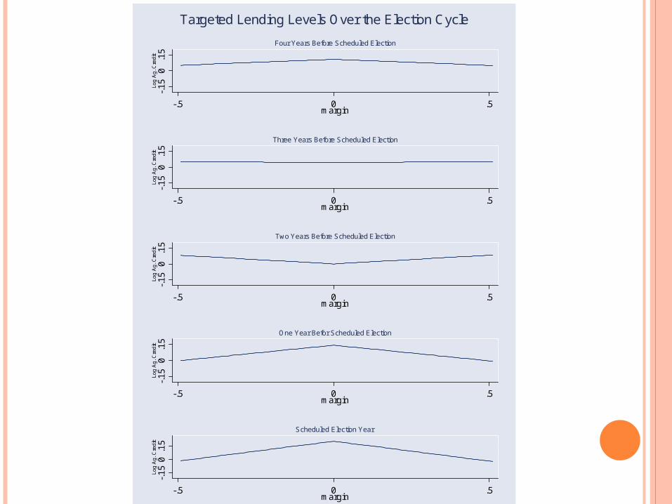
Note: The panels in the figure graph the predicted relationship between agricultural credit levels frompublic sector banks and political support of the state majority party. Each panel gives the relationship for a different year in the electoral cycle.

Targeted Lending Levels Over the Election Cycle

INTERPRETING COEFFICIENTS

Standard deviation of absolute margin of victory is .11 Moving from a district with a margin of victory of

0 to a margin of victory of .11 reduces the size of the cycle by approximately 5 percentage points

-.0

4-.

02

0.0

2.0

4.0

6

-4 -3 -2 -1 0Years Until Scheduled Election

Public Banks

-.4

-.2

0.2

.4

-4 -3 -2 -1 0Years Until Scheduled Election

Private Banks

Note: Predicted agricultural credit for a notional district in which the margin of victory in theprevious election was fifteen. Dotted lines give the 95 percent confidence interval.

Figure 3: Cycles in Level of Credit, Non-Swing District-.

050

.05

.1

-4 -3 -2 -1 0Years Until Scheduled Election

Public Banks

-.4

-.3

-.2

-.1

0

-4 -3 -2 -1 0Years Until Scheduled Election

Private Banks

Note: Predicted agricultural credit for a notional district in which the margin of victory in theprevious election was zero. Dotted lines give the 95 percent confidence interval.

Figure 2: Cycles in Level of Credit, Swing District

TARGETED ALLOCATION (CONCLUDED)

Evidence consistent with “swing voter” models; patronage and programmatic redistribution can be ruled out

Government ownership of banks introduces distortions in credit (but cannot yet make welfare statements)

DO ELECTIONS AFFECT LOAN REPAYMENT? Challenges

Do not observe panel of loans, only district aggregate

Evidence of cycles in repayment

suggest costliness

Use “more than 6 months” late as indicator for defaultMany agricultural loans are for

harvest/season

Table 7

Lending Cycles and Non-Performing Loans

Table 8 Examine being late on loans.

ELECTIONS AFFECT LOAN REPAYMENT

There are cycle in loan repayment rates

Suggests electoral cycle is costly Enforcement is more lax in election years The marginal electoral loan may be more likely

to default Non-performing loans are written off following an

election

DO POLITICAL LOANS AFFECT OUTPUT

Data - Agricultural Output at the state level, 1992-1999 Log real value of agricultural output

Election Schedule serves as instruments for agricultural credit

DO POLITICAL LOANS AFFECT OUTPUT?FIRST STAGE & REDUCED FORM/ IV Table 9

Look at output and credit. Panel A is reduced form and Panel B is IV.

OUTPUT CONCLUSION

No measurable effect on output

TWO

FOUR

CONCLUSION

Combining theories of political cycles and tactical transfers helps identify manipulation of public resources Agricultural lending exhibits substantial lending

cycles Lending is targeted in election years, not in non-

election years Results unlikely to be caused by omitted factors Private banks do not exhibit these distortions

CONCLUSION

Combining theories of political cycles and tactical transfers helps identify manipulation of public resources Agricultural lending exhibits substantial lending

cycles Lending is targeted in election years, not in non-

election years Results unlikely to be caused by omitted factors Private banks do not exhibit these distortions

LESSONS

Strong evidence for “Political” view of government involvement in bank credit

Evidence against “Development” view Explains why politicians favor public banks,

and agricultural credit in particular Politicians may care more about re-election

than delivering patronage to core supporters

WHAT DO FIRMS DO WITH CASH WINDFALLS?Blanchard, Lopez-de-Silanes, and Shleifer

JFE 1994

MOTIVATION

How does one provide evidence of investment policy, internal opportunities, and cash flow sensitivity?

What do firms do with cash windfalls when investment opportunities are unchanged? In perfect capital markets, would give money

back to shareholders if holding cash inside firm is tax disadvantaged.

In imperfect capital markets: If firm was capital constrained, should increase

investment in projects it couldn’t do. If managers pursue their own objectives, then could

get very perverse behavior.

DATA Process of identifying cash windfall firms is

quite selective: Looked in WSJ index for mentions of “Antitrust”,

“Patents”, and “Suits” from 1980 to 1986. Find 110 firms that won awards

(Easier today with the web and ability to electronically search news.)

Use four criteria to create sample: Should not affect firm’s marginal Q Award should be significant Require 10K and proxies. Focus only on award winners.

Final sample is 11 firms. Table 1.

SIGNIFICANCE OF AWARD

Table 2 Look at award as fraction of sales and assets.

Table 3 Look at main line of business Look at firm Qs, sales, investment, and debt.

Subtract size of award from Q. These are pretty bad firms with poor investment

opportunities.

MARKET’S REACTION

Do event study. Don’t know the exact amount of

leakage/anticipation of award. Look at CARs centered on award date for firms:

100, 10, and 3 days. Deflate market value change imputed by the

CAR by the size of the award. In general, increase in market cap is small fractio

nof award. Interpretation.

Award is wasted. Award is anticipated.

INVESTMENT

Look at change in investments pre and post award.

Deflate change in investment rate by assets or net award.

Table 6. Small increases in investment on average. Jamesbury is interesting example.

Starts constructing new plant.

ASSET SALES AND ACQUISITIONS

Table 7. Not much asset sales.

Table 8. More troubled firms seem to buy assets. DASA (formerly a telecomm equipment

company) buys oil wells and credit collection business.

UNC quires a communications carrier and starts air services like pilot training.

CHANGE IN FINANCIAL POLICIES

Look at change in debt pre and post-award. Firms seem to add debt after award.

Table 9. Consistent with either commitment to pay out

cash or increase in debt capacity. Look at payout policy.

No increase in dividends. Increase in repurchases – Table 10. Repurchases tend to be targeted at large

investors. Reduction in oversight.

EXECUTIVE COMPENSATION

Look at changes in executive compensation. Cash and stock compensation. Table 11 – Looks like increases in cash primarily.

CONCLUSIONS

Examination looks like cash windfalls are typically used to entrench management.

Increase in pet projects, acquisition. Increase in exec comp. Targeted repurchases.

Methodology is interesting in approach of trying to cleanly identify sample. One more table than data points.

CASH FLOW AND INVESTMENT: EVIDENCE FROM INTERNAL CAPITAL MARKETSOwen Lamont

JF 1997

MOTIVATION

Similar to Blanchard, et al., trying to identify group of firms that have change in cash flow and see how it affects investment.

Want a shock that is unanticipated (exogenous) and its affect on multi-divisional firms that have businesses whose prospects are uncorrelated with the other division’s prospects.

Natural experiment: Oil shock of 1986.

Severe and rapid real price decline in oil prices. Look at diversified oil companies who had other

businesses unrelated to oil.

INTERNAL CAPITAL MARKETS

If external finance is costly, then internal capital markets can allocate money across divisions to overcome some of the financing wedges that exist between internal and external cash.

If capital markets were perfect, would expect no change in investment with a decline in the unrelated segment cash flow.

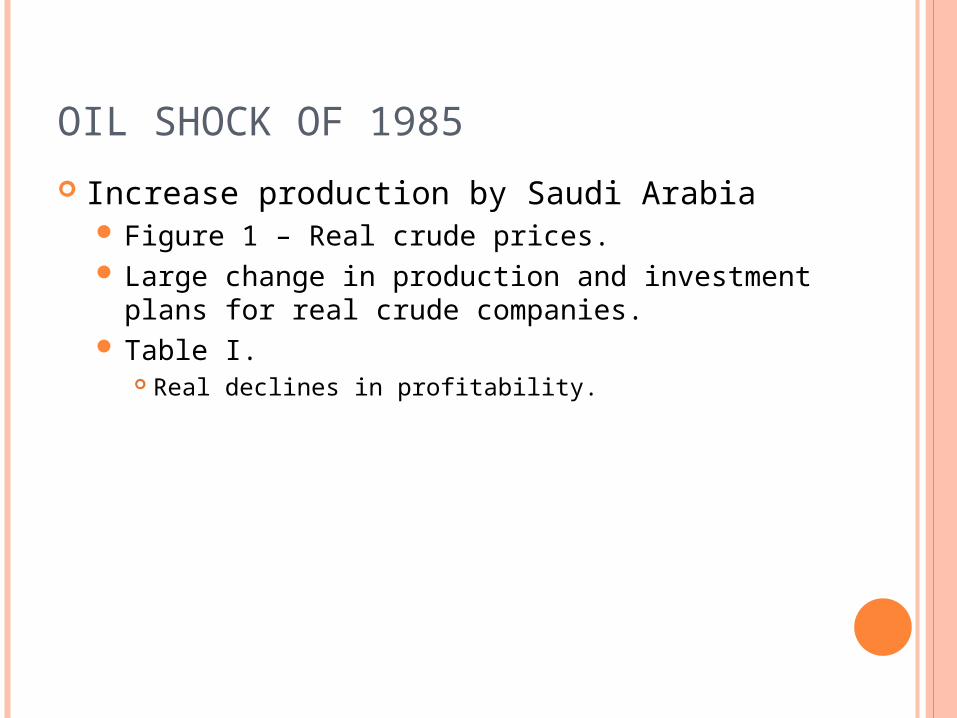
OIL SHOCK OF 1985

Increase production by Saudi Arabia Figure 1 – Real crude prices. Large change in production and investment plans

for real crude companies. Table I.

Real declines in profitability.

SAMPLE

Look at multi-segment reporting firms. Issue with multi-segment firms.

Firms report segments that are more than 10% of firm revenues.

Reporting is endogenous. Can change from year to year. Does not necessarily represent how firm is organized.

Extract all firms from Compustat in 1985 that had either their primary or secondary SIC code in oil and gas extraction (SIC code 13). Firms classified as oil-dependent if at least 25% of their

cash flow came from oil extraction.

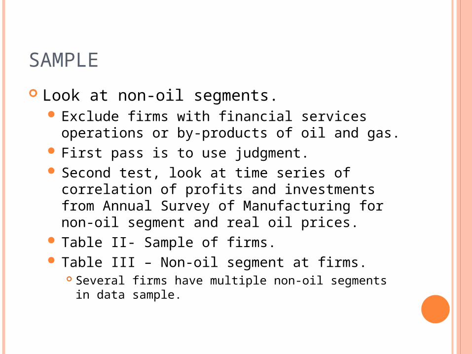
SAMPLE

Look at non-oil segments. Exclude firms with financial services operations

or by-products of oil and gas. First pass is to use judgment. Second test, look at time series of correlation of

profits and investments from Annual Survey of Manufacturing for non-oil segment and real oil prices.

Table II- Sample of firms. Table III – Non-oil segment at firms.

Several firms have multiple non-oil segments in data sample.

TESTS

Examine investment pre- and post-oil shock for non-oil segments. Table V – Raw and industry adjusted investment

for non-oil segments.

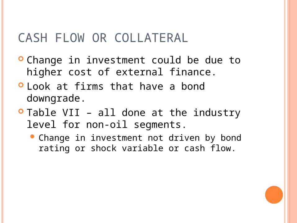
CASH FLOW OR COLLATERAL

Change in investment could be due to higher cost of external finance.

Look at firms that have a bond downgrade. Table VII – all done at the industry level for

non-oil segments. Change in investment not driven by bond rating

or shock variable or cash flow.

OVER OR UNDERINVESTMENT

Testing between capital market imperfection (underinvesment after shock) vs. agency costs (overinvestment prior to shock). Look at industry adjusted investment rates. Table VIII

Go from roughly average/median to below industry average/medians.

Table IX Look at profitability. Non-oil segments were less profitable than industry

averages prior to shock and then increase to average after shock.

SUBSIDIES TO NON-OIL DIVISIONS

Table X. Cut deepest for divisions in which CF<I prior to

shock. Also, look at segment investment as a

function of oil cash flows to firm sales. Table XI

OBSERVATIONS

Appears that diversified oil companies subsidize non-oil divisions with free cash flow generated by the oil profits.

This subsidization appears to be the results of agency costs.

More generally, nice natural experiment to provide evidence of investment behavior within firms.

ENJOYING THE QUIET LIFE? CORPORATE GOVERNANCE AND MANAGERIAL PREFERENCESBertrand and Mullainathan

JPE 2003

MOTIVATION

Managers typically own very little of their company stock. 90% own less than 5% (Ofek and Yermack

(2000)) Are managers who are entrenched empire

building (Williamson (1964) vs. quiet life consumers (Hicks (1935))?

Lots of studies look at the relationship between measures of corporate governance and firm performance/activities. But internal governance is endogenous.

Firms choose what level of shareholder protection, etc. they have.

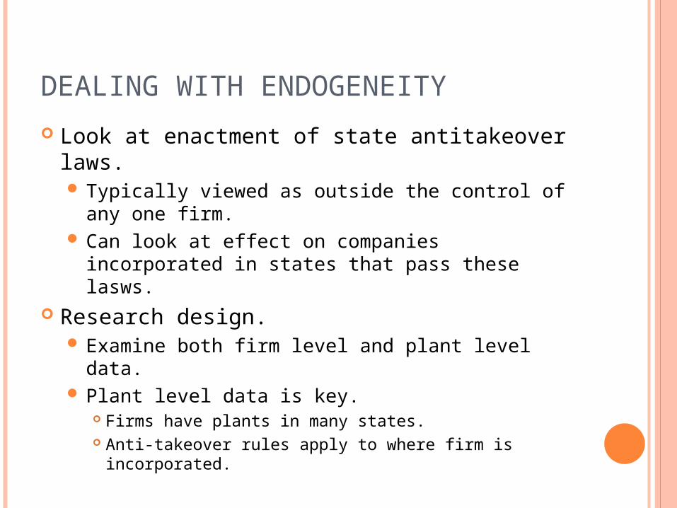
DEALING WITH ENDOGENEITY

Look at enactment of state antitakeover laws. Typically viewed as outside the control of any

one firm. Can look at effect on companies incorporated in

states that pass these lasws. Research design.

Examine both firm level and plant level data. Plant level data is key.

Firms have plants in many states. Anti-takeover rules apply to where firm is incorporated.

STATE ANTI-TAKEOVER LAWS

Good history of first and second generation anti-takeover laws.

Table 1. List of states and years that the laws passed.

Focus on Business Combination Laws Moratorium (3 – 5 years) on specified transaction

between target and a raider holding a certain % of the stock unless board votes

Literature on impact of laws. Stock price reaction – small negative.

Hard to pin down date. Evidence on actual takeover incidence is mixed.

PAPER’S STRATEGY

Use difference in differences comparisons between states that adopt BC laws and those that don’t.

Have data at the firm level and the plant level. Can control for local economic conditions.

DATA

LRD – Longitudinal Research Datafile Census – large probability sample of US

manufacturing firms Have data on individual plants. Matched to Compustat

Issue with Compustat – has only most recent state of incorporation, i.e., it is not historical.

VARIABLES

Average hourly production worker wage Capital stock Return on capital Plant births and deaths Table 2 – Summary stats

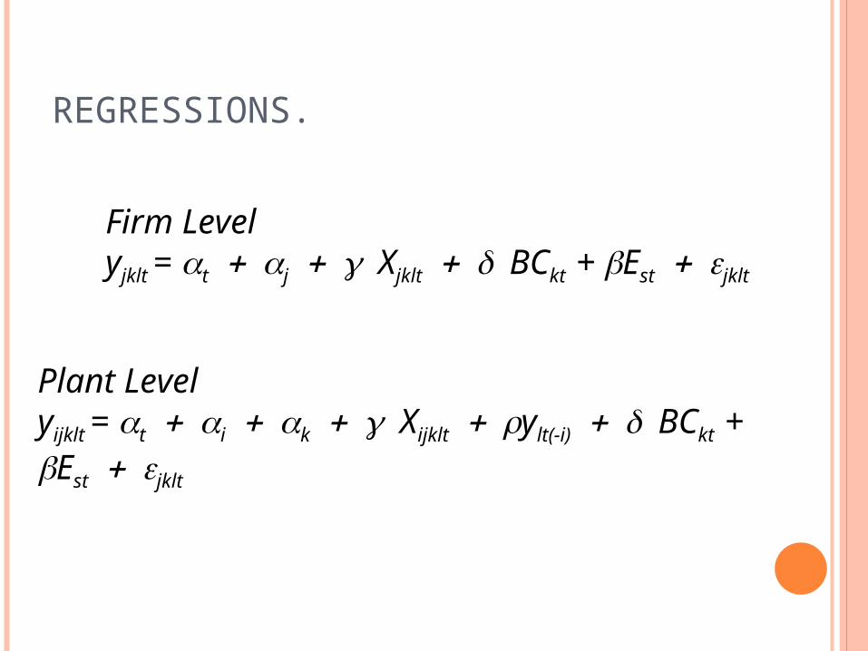
REGRESSIONS.

Firm Levelyjklt = tjXjkltBCkt + Estjklt

Plant Levelyijklt = tikXijkltylt(-i)BCkt + Estjklt

WAGES.

Do managers increase wages after BC law? Why would they increase wages above profit

maximizing levels? Reduce turnover. Reduce complaints. Allow for clustering at the state of location level

to adjust for serial correlation. Table 3

Column 5 – look at reverse causality.

PLANT BIRTHS AND DEATHS

Look at death of plants Table 5 – lower rate of plant closings.

Plant births. Table 6 – BC law decreases plant birth by 2%.

Large relative to unconditional plant birth probability of 7%.

No effect on capex or firm size – Tables 7 and 8.

PRODUCTIVITY

Seems as if managers are paying higher wages and being less aggressive.

Does this affect plant level performance. Look at TFP

TFP is the residual from this regression. Second measure of productivity is the return

on capital.

log(output) = tlog(wage billi log(capitali log(materialii

REGRESSIONS

Table 9 Results appear to show lower productivity when

TFP percentiles are measuresd. Marginal effect on return on capital.

OBSERVATIONS

Results consistent with managers that are insulated from takeover “enjoying the quiet life”

Good natural experiment. Lots of interesting variation and results. Exploits location/incorporation differences. Nice data set on plant level variables.

DOES CORPORATE GOVERNANCE MATTER IN COMPETITIVE INDUSTRIESGroud and Mueller

Working paper 2007

IDEA

Notion that market competition weeds out firm inefficiencies.

Would expect that corporate governance is less important when firms face highly competitive markets.

Do the Bertrand Mullainathan analysis, but add in the level of competition in the industry. Expect that in highly concentrated industries, the

Bertrand/Mullainathan result would be particularly strong.

Not so in highly fragmented/competitive industries.

DATA

Main data is Compustat: Exclude utilities – regulated. Use state of location and state of incorporation.

Not necessarily the same thing. Table I – Summary Compute 3-digit Herfindahl index.

Test robustness at 2 and 4 digit. Industry definition is particularly tough.

SIC codes not very good for high technology companies.

Mapping to actual competitors may be problematic.

MAIN APPROACH

Use differences in differences Look at operating performance about how it

depends upon concentration

yijklt =tiXijkltBCktHerfindahljt(BCkt x Herfindahljtjklt

CAVEAT

Not looking at LRD data Looking at Compustat Table III – Look at ROA/assets

BC alone associated with lower ROA Once interaction term put in, all the effect of BC

is due to concentrated industries Standard errors are clustered at the state level to

deal with serial correlation of residuals at the state level.

MEASUREMENT ERROR

Perhaps Herfindahl is measured with error. Imprecise industries Wrong measure of competitiveness.

Use dummy variable for Herfindahl above and below the median or with three Herfindahl dummies. No dependent upon functional form of the

Herfindahl. Table IV.

ROBUSTNESS CHECKS

Use past Herf to control for reverse causality – Table VII.

Look at alternative performance measures – Table VIII.

Look only at manufacturing – Table IX. Alternative correction from Bertrand, Duflo,

and Mallainathan (2004) – Table X.

EVENT STUDY

Try to replicate Karpoff and Malatesta (1989) Difficulty

When is first announcement? What date do you use? What is the market expectation through time?

Look for first announcement of the law. Exhaustive search where possible. Only find news stories about 19 of the 30 laws. But this covers the big states.

EVENT STUDY ISSUES Typical event study methodology assumes

that all events are independent. Solutions:

Typically, just form portfolios of affected and non-affected firms.

Here, authors form equally weighted portfolios of firms that are incorporated in the state and run market model on equally weighted CRSP market portfolio.

Estimate model for days -241 to -41. Get factor loadings. Create predicted returns and subtract from

actual return.

EVENT STUDY

Look at CARs for days -40 to -, -3 to -2, -1 to 0, 1 to 2 and 1 to 10.

Separate out firms based upon Herfindahl in the previous groups.

Table XII. Biggest price drop is in the concentrated

industries. BC laws affect performance of the concentrated

firms that face less competition.

CONTRIBUTION

Interesting extension of prior work. Thoughtful methodology.