Cross Section Generation Strategy for High

Conversion Light Water Reactors

Bryan Herman and Eugene Shwageraus

1Department of Nuclear Science and Engineering

Massachusetts Institute of Technology

77 Massachusetts Ave; Cambridge, MA 02139

Email: bherman@mit.edu

Outline

High Conversion Water Reactors

Cross Section Homogenization Process

Branch Cases

Application of Discontinuity Factors

Conclusions/Future Work

Serpent Wish List

High Conversion Water Reactors

Parfait core

Axial blankets are used to achieve BR~1.01

Blankets: Depleted or Natural Uranium

Fissile zones: TRU (Pu+MA) MOX

Examples:

Hitachi – Resource Renewable Boiling

Water Reactor (RBWR)

JAEA – Reduced Moderation Boiling Water

Reactor (RMWR)

Hitachi RBWR

Assemblies are axially heterogeneous

Core average void fraction ~60%

vs. typical BWR ~40%

Fissile zones produce neutrons while

blanket zones absorb them

Significant axial streaming of neutrons

Lower Reflector

Lower Fissile

Internal Blanket

Upper Fissile

Upper Blanket

Upper Reflector

Lower Blanket

Cross Section Homogenization

Serpent

PARCS

Obtaining Homogenized XS

PARCS solves multi-group diffusion eq.:

macroscopic cross sections are flux weighted:

−𝛻 ⋅ 𝐷𝑔𝛻𝜙𝑔 + Σ𝑎𝑔∗𝜙𝑔 + 𝜐Σ𝑠𝑔𝜙𝑔 = 𝜐Σ𝑠

ℎ→𝑔𝜙ℎ

ℎ

+𝜒𝑔

𝑘𝑒𝑓𝑓 𝜈Σ𝑓,ℎ𝜙ℎ

ℎ

leakage interactions scattering production

w/ (n,xn) production

fission

production

Σ𝛼𝑔 = 𝑑𝐸 𝑑3𝑟 Σ𝛼 𝑟 , 𝐸 𝜙 𝑟 , 𝐸𝑉

𝐸𝑔−1𝐸𝑔

𝑑𝐸 𝑑3𝑟 𝜙 𝑟 , 𝐸𝑉

𝐸𝑔−1𝐸𝑔

Monte Carlo Estimation of D

Diffusion coefficient must be current-weighted

Usually it is just flux-weighted and a B1 calculation

is performed to adjust it

For RBWR we would like to have directional

diffusion coefficients

Instead we use discontinuity factors to

preserve neutron balance

PARCS Overall Methodology Serpent

PARCS SerpentXS

Branch Cases Must account for a range of operating conditions

unknown beforehand

Cross sections are therefore parameterized over

instantaneous values and time-averaged (history)

operating conditions

Instantaneous conditions – control rod, poison conc.,

coolant density, fuel temp, coolant temp

Histories – burnup, control rod, density …

SerpentXS Code

PWR Test Problem Branch Indx CR DC

[g/cc]

PC

[pcm]

TF [K] TC [K]

Refer. 1 0 0.707 1000 900 582

CR 1 1 0.707 1000 900 582

DC low 1 0 0.594 1000 900 582

DC high 2 0 0.740 1000 900 582

TF low 1 0 0.707 1000 582 582

TF high 2 0 0.707 1000 1500 582 Reference Geometry

Rodded Geometry

Power Distribution

Reference Case

Fuel Temperature Branch

2-D vs. 3-D Generated XS

Strong axial material discontinuities

Obtain XSs generated in conventional 2-D

geometry (denoted as 2-D XSs)

Surrounded by zero-net current boundaries

Compare to XSs generated for axial zones

surrounded by neighbors (denoted as 3-D

XSs)

Serpent makes this relatively simple

2-D vs. 3-D XS

Homogenize Homogenize

2-D 3-D

Fissile-Fissile Two-Zone Results

Keff = 1.55908

2-D:

Keff = 1.55900

3-D:

Keff = 1.55913

Fissile-Blanket Two-Zone Results

Keff = 1.36620

2-D:

Keff = 1.37733

3-D:

Keff = 1.38312

Axial Discontinuity Factors

Two-Zone Problem

K-eff: 1.36620

PARCS (No ADFs):

K-eff: 1.38312

J J

Get Homogeneous Flux

UB2

UF2

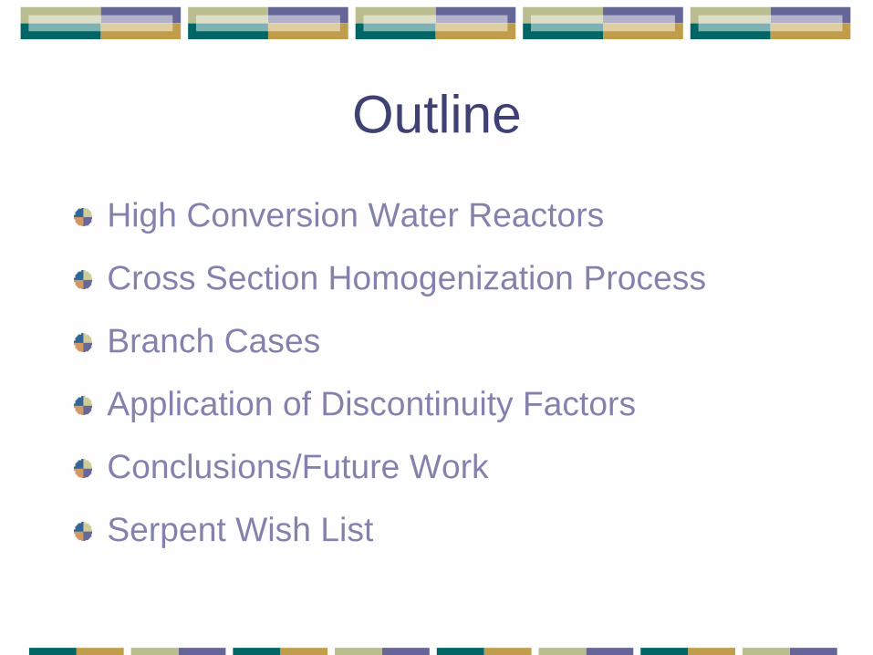
Discontinuity factors: Background

Real flux has to be continuous

Homogeneous flux does not

ADF: Ratio of heterogeneous-to-homogeneous surface flux

Conventional process: 2D reflected assembly

Homogeneous surface flux = nodal flux

Surface current is zero

NOT the case in RBWR

Procedure for toy problems

Obtain the heterogeneous solution with Serpent

Global reflective boundaries,

Extract homogenized parameters from Serpent

Compute interface currents using neutron balance

Perform fixed source 1D diffusion calculation for each coarse

region

Compute discontinuity factors using surface fluxes:

Heterogeneous (Serpent)

Homogeneous (Fine mesh 1D diffusion)

Run the entire homogeneous geometry (1D diffusion + ADFs)

To verify that homogeneous and heterogeneous setups are equivalent

Axial Discontinuity Factors

f1UF = 1.028 f1

UB = 0.966

f 2UF= 0.972 f2

UB = 1.034

Discontinuity Factors

PARCS (ADFs):

K-eff: 1.36620

The need for surface current

tallies… To generate the exact discontinuity factors (e.g. in

reflector) surface currents are needed

Homogeneous flux is determined from fixed source

diffusion equation with current boundary conditions

Currently we use global reflective boundary

conditions to back out surface currents using neutron

balance

2-G Single Assembly

Calculations

12-G Single Assembly

Calculations

Approximation of ADFs

Can we get away with just homogenizing over

two-zone problems

Conclusions

Observed large differences between Serpent and

PARCS calculations using conventional approach

Need to treat axial discontinuity for RBWR core

Current methods are not appropriate

Developed methodology to generate cross section

database for PARCS

Showed applicability of axial discontinuity factors

Future Work

Finish developing methodology for axial discontinuity

factors

Study sensitivity of discontinuity factors for different

operating conditions

Approximate discontinuity factors with:

Single Assembly Full Core

Serpent “Wish List”

Surface current tallies (a must)

A parallel calculation method that reproduces

answers w/ arbitrary number of CPUs

Built-in method to restart calculations and perturb

conditions (like in CASMO)

Output fission product yields (I, Xe, Pm)

Pin power and flux distribution per energy group

Acknowledgments

• Thesis supervisors

• Prof. Eugene Shwageraus

• Prof. Ben Forget

• Prof. Mujid Kazimi

• Prof. Smith for discontinuity factors

• Prof. Downar (UMich) for PARCS

• Dr. Jaakko Leppanen (VTT Finland) for Serpent

• Rickover Fellowship

References

Downar, T., Lee, D., Xu, Y., and Seker, V. (2009). PARCS v3.0: U.S. NRC Core Neutronics

Simulator. User Manual. University of Michigan.

Leppänen, J. (2007). Development of a New Monte Carlo Reactor Physics Code. PhD thesis,

Helsinki University of Technology.

Smith, K. S. (1980). Spatial Homogenization Methods for Light Water Reactor Analysis. PhD thesis,

Massachusetts Institute of Technology.

Stalek, M. and Demazière, C. (2008). Development and validation of a cross-section interface for

PARCS. Annals of Nuclear Energy, 35:2397–2409.

Takeda, R., Miwa, J., and Moriya, K. (2007). BWRs for Long-Term Energy Supply and for

Fissioning almost all Transuraniums. Boise, Idaho. Proc. Global 2007.

Xu, Y. and Downar, T. (2009). GenPMAXS-V5: Code for Generating the PARCS Cross Section

Interface File PMAXS. University of Michigan.

Questions