Cross Hedging with Single Stock Futures

July, 2006

The authors:

Chris Brooks is a Professor of Finance at the ICMA Centre, University of Reading,

UK. Ryan J. Davies is an Assistant Professor and the Lyle Howland Term Chair in

Finance at Babson College, Massachusetts. Sang Soo Kim is the Head of Commodity

Derivatives at Korea Development Bank.

Acknowledgements:

A previous version of this paper was circulated under the title “Reducing basis risk

for stocks by cross hedging with matched futures”. We are grateful for comments

received from an anonymous referee of this journal, and to seminar participants at

University College Dublin, Babson College, and the 2005 Northern Finance

Association meetings. The views expressed in this paper are those of the authors and

do not necessarily reflect those of The Korea Development Bank.

§ rdavies@babson.edu; Tel: (781) 239-5345; Fax: (781) 239-5004 (Corresponding Author)

Chris Brooks

ICMA Centre University of Reading

Whiteknights Reading RG6 6BA

UK

Ryan J. Davies§

Finance Division Babson College Tomasso Hall

Babson Park, MA 02457-0310

USA

Sang Soo Kim

Korea Development Bank 16-3 Yeoido-dong Yeongdeungpo-gu Seoul, Korea 150-973

2

Cross Hedging with Single Stock Futures

Abstract

This study evaluates the efficiency of cross hedging with single stock futures

(SSF) contracts. We propose a new technique for hedging exposure to an individual

stock that does not have options or exchange-traded SSF contracts written on it. Our

method selects as a hedging instrument a portfolio of SSF contracts which are

selected based on how closely matched their underlying firm characteristics are with

the characteristics of the individual stock we are attempting to hedge. We investigate

whether using cross-sectional characteristics to construct our hedge can provide

hedging efficiency gains over that of constructing the hedge based on return

correlations alone. Overall, we find that the best hedging performance is achieved

through a portfolio that is hedged with market index futures and a SSF matched by

both historical return correlation and cross-sectional matching characteristics. We

also find it preferable to retain the chosen SSF contracts for the whole out-of-sample

period while re-estimating the optimal hedge ratio at each rolling window.

Keywords: Single stock futures, hedging, Universal Stock Futures, OneChicago.

1

1 Introduction

There are a variety of reasons why retail and institutional investors may have

substantial undiversified exposures to single stocks.1 For example, an investment

bank may acquire shares through syndication that are subject to a covenant

restricting their sale. Similarly, an investor may hold stock options that are currently

deep in the money but for which selling is not permitted for a prescribed period. Or,

a fund manager may have a large exposure to a stock that he does not want to close

out. In all of these cases, the investor may desire to hedge, rather than sell, his shares

as protection against price falls.

One way that an investor could deal with such a problem is to enter into an

offsetting short position. Short selling is likely to be a high cost tool because of its

associated margin requirements, up-tick trading restrictions, loan interest, and

potential risk of a short squeeze. As well, there are potential problems locating a

stock to borrow and, for retail investors there a significant risk of the stock being

unexpectedly recalled. As an alternative, the investor could use stock options. This is

often impractical, however, since the vast majority of listed stocks do not have

exchange-traded options written on them and over-the-counter option markets are

often not directly accessible to retail investors. Furthermore, the prices of over-the-

counter options are less transparent and may be subject to a (substantial) premium

based on the presence of an intermediary and/or the nature of the bilateral

relationship between the counterparties (see Duffie, Gârleanu, and Pedersen (2005)).

Futures contracts are likely to represent a much cleaner hedging tool. Futures

contracts have no premium, low transaction costs, low margin requirements, and

more transparent pricing than over-the-counter options. Hedging with stock index

futures is certainly easy and cost-effective, but may provide an inadequate hedge if

the returns profile of the stock exposure is significantly different to that of the index

as a whole. As an alternative, one may consider hedging with single stock futures

(SSF) contracts. Such a hedge is likely to work well if there is a traded future on the

required stock. In cases for which the required SSF contract does not exist, the

investor faces a choice: hedge with a stock index or cross-hedge using the futures

contract of a closely related stock. Since cross-hedging efficiency is degraded by the

inevitable ‘basis risk’, it is essential to select the appropriate futures contract

1 Goetzmann and Kumar (2005) explore some of the reasons why individual investors hold under-

diversified portfolios. Kahl, Liu, and Longstaff (2003) examine the welfare effects of restrictions on the sale of compensation-based stockholdings.

2

carefully and to develop an effective cross-hedging model.

To this end, the objective of this study is to evaluate the efficiency of cross

hedging with the new SSF contracts introduced in the U.S. in November 2002. At the

end of June 2006, 202 individual U.S. stocks had SSF contracts written on them. To

cross hedge other stocks, we propose using a technique that matches the spot stock

with one or more of the available SSF contracts in a manner designed to reduce the

basis risk of cross hedging and to obtain the most efficient hedging portfolio.

The benefits of hedging with futures have been well studied, and cross hedging

with futures has been successfully used in various financial markets including

commodity (Foster and Whiteman, 2002; Franken and Parcell, 2003), foreign

exchange (Brooks and Chong, 2001) and equity markets. While there has been

extensive testing of the various econometric models available to estimate the optimal

hedge ratio, there has been little research on how to select optimally the hedging

asset. If the futures contract for the specific individual stock does not exist, then the

investor is forced to cross-hedge. The effectiveness of the hedge may depend more

crucially on the selected futures contract than on the optimality of the estimated

hedge ratio. If the hedging asset is chosen to maximize the correlation between the

spot returns and futures returns, by definition, this will ensure that the basis risk

from cross-hedging is minimized (in-sample). We implement such a scheme in this

paper, but as we argue below and show empirically, we may be able to reduce better

the out-of-sample basis risk by selecting a futures contract using a measure other

than the correlation of its returns with those of the spot asset.

The hedging efficiency of conventional estimation models of the optimal hedge

ratio depends on the return covariance between the spot and hedging assets. As the

estimated hedge ratio and resulting efficiency are contingent on the sample period

and its length, there is no guarantee that an effective hedge will continue over a

different time horizon. Unfortunately, there is no universally accepted objective

decision criterion for the appropriate length of the sample period.

As an alternative, one could consider the common fundamental factors that affect

the price movement of the spot asset and the hedging asset. In the context of cross

hedging, if two assets have similar fundamental factors that determine their

subsequent price movements, then the resulting hedge can be expected to be

relatively effective. We would argue that fundamental characteristics are, by their

very nature, likely to vary much less from one sample to another than returns, and

3

should therefore lead to more stable and more accurate hedging ratios. We propose a

new hedging technique, based on matching the spot asset with the ideal hedging

asset(s) using nonparametric sample matching techniques that control those

fundamental factors as the matching characteristics. The resulting hedged portfolio

should minimize the basis risk. We show that using matching techniques to

construct the hedged portfolio can provide efficiency gains over a hedged portfolio

constructed purely according to the correlation between the futures and spot returns.

It may be problematic to estimate accurately correlation using a finite sample of

historical returns data for the spot and futures assets. The noise inherent in these

returns, and the resulting correlation estimates, means that it may not be desirable to

select the hedging asset on the basis of the correlation. In contrast, if we are able to

capture a measure of the “fundamental” value of the firm, it should by definition be

more stable over time and therefore less prone to measurement error, enabling us to

more reliably determine the appropriate futures contract.

The literature on factors driving individual stock returns is vast. There are a

number of different measures of firm fundamentals that could be employed, but

many are based on quantities that are only observable on an annual or biennial basis

(such as earnings or dividends), which would provide too few observations. Instead,

our choice of factors (industry, beta, market capitalization, and price to book ratio) is

in the same spirit as the factors proposed by Fama and French (1993). The Fama-

French factors have become highly popular as risk attribution measures in the asset

pricing literature, and have been the most successful in explaining the cross-sectional

variation in returns. Our factors can also be motivated by classic papers such as Banz

(1981), who find a relation between firm size and returns, and Rosenberg, Reid, and

Lanstein (1985), who find a relation between the price / book ratio and returns.

Our method is supported by recent evidence that individual stocks often move

together, allowing one stock (or its associated single stock futures contract) to

provide a natural hedge for another. For example, Gatev, Goetzmann, and

Rouwnhorst (2005) investigate the following “pairs trading” strategy: (i) the investor

first finds two stocks that have historically moved together; (ii) when their prices

diverge the investor shorts the winner and buys the loser; (iii) eventually, the prices

(hopefully) converge again, generating profits. Gatev, et al. show that this simple

strategy produces significant positive risk-adjusted returns.2 Additional support for

2 Gatev, Goetzmann, Rouwnhorst (2005) form pairs over a 12-month period and trade them in the next 6-month period. They choose a matching partner for each stock by finding the security that

4

our methodology is provided by Tookes (2004). She shows in the context of earnings

announcements, that returns in the stocks on non-announcing competitors have

information content for announcing firms.

For our empirical analysis, we construct four types of cross-hedged portfolios

that are hedged with: i) single SSF only, ii) single SSF and market index futures, iii)

multiple SSF contracts, and iv) multiple SSF contracts and market index futures.

Each futures contract is chosen according to three different characteristic sets. The

first matching characteristic set consists of only historical return correlations

between spot and potential futures implied in the conventional cross hedging model.

The second set consists of possible fundamental factors (industry, beta, market

capitalization, and price to book ratio) that influence the price movements of stocks.

The last set includes both return correlations and fundamental factors. Finally, we

repeat the same analysis with the additional restriction that the selected SSF

contracts are from the same industry as the spot stock.

To examine the hedging efficiency of each hedged portfolio, we consider the

percentage reduction of the variance of the hedged portfolio relative to that of the

unhedged portfolio. To compare the out-of-sample hedging efficiency of each model

over time, we construct a hedged portfolio with a 1-day life and roll it over with

fixed sized time windows. Overall, we find that the best hedging performance is

achieved through a portfolio that is hedged with market index futures and a SSF

matched by both historical return correlation and cross-sectional matching

characteristics. We also find it preferable to retain the chosen SSF contracts for the

whole out-of-sample period while re-estimating the optimal hedge ratio at each

rolling window.

The paper is organised as follows. The next section describes the SSF markets and

provides an overview of existing research on SSFs. Section 3 outlines our

methodology for estimating the hedge ratio and determining hedging efficiency.

Section 4 outlines the various cross-hedging models based on different hedging

strategies and explains the estimation procedure and rebalancing methods. Section 5

describes the data. Section 6 presents the estimation results and finally, Section 7

concludes.

minimizes the sum of squared deviations between the two normalized price series. They also present results by sector, where they restrict both matched stocks to belong to the same broad industry categories.

5

2 The Single Stock Futures Market

U.S.-listed single stock futures became possible with the Commodity Futures

Modernization Act of 2000. This act repealed the so-called Shad-Johnson Accord,

which had banned SSF, in part because of regulatory concerns about the leverage

effect of SSF and possible manipulation of the underlying spot stock price. They are

regulated jointly by both the Commodity Futures Trading Commission (CFTC) and

the Securities and Exchange Commission (SEC). This joint regulation regime has

been heavily criticized by many as unworkable, including by Johnson (2005) – one of

the authors of the Shad-Johnson accord. Knepper (2004) provides an opposing

viewpoint in favor of the current regulatory regime.

The approval of listing standards and margin requirements by the SEC and the

authorization of trading rules by the CFTC paved the way for the November 8, 2002

launch of the first U.S.-based SSF markets: OneChicago and Nasdaq.LIFFE (NQLX).

OneChicago is a joint venture of the Chicago Board Options Exchange, the Chicago

Mercantile Exchange, and the Chicago Board of Trade. 3 Soon after launch,

OneChicago quickly became the dominant trading venue for SSF contracts in the US

and is thus the focus of this study. NQLX ceased operations in December 2004.

There are several possible reasons for the relative success of OneChicago

compared with NQLX. One possibility is differences in market structure.

OneChicago selected a lead market maker model, in which the market maker

provides continuous two-sided quote prices and ensures liquidity. This market

model contrasted with the combination of a multiple market maker system and a

central order book adopted by the now defunct NQLX. The relative success of

OneChicago may also be due to the choice of initial products listed on the two

markets. Ang and Cheng (2005b) examine how OneChicago and NQLX selected

their initial listed products. They obtain estimates of an underlying stock’s SSF

listing probability and show that this probability is a good predictor of post-listing

success.

There are many potential benefits of single stock futures. One benefit is that SSFs

have lower margin requirements than equity. The Federal Reserve’s Regulation T

sets the standard initial and maintenance margin requirement of 20% for SSFs, both

long and short positions. This is much lower than the 50% initial requirement for a

3 On March 16, 2006, it was announced that Interactive Brokers, LLC would make a significant equity

investment in OneChicago resulting in a 40% ownership share.

6

long equity position and the 50% plus sale proceeds requirement for a short equity

position. Long and short equity positions on margin also have a higher maintenance

margin requirement of 30%.

Another benefit is that SSFs enable easier short selling, with the ability to sell on a

downtick and the elimination of the need to use a stock loan department. In order to

reduce the risk of a short squeeze in SSFs, the CFTC introduced speculative position

limit levels for SSFs based on the average daily trading volume of the underlying

security.4 As well, lower maintenance margin requirements reduce the risk of a

forced margin call and the forward looking nature of SSF contracts helps moderate

the impact of short-term price movements in the underlying security.

Other benefits of SSFs include their usage for spread trading and their ability to

isolate a stock from an index. As well, SSFs can provide a cleaner, more efficient

hedging tool than options. There is a well-defined no-arbitrage relation linking

futures prices with the price of the underlying. This contrasts with option prices

which depend critically on subjective assumptions about underlying price volatility.

In addition to the US markets, single stock futures have recently been introduced

in many exchanges around the world; including Hong Kong, London, Madrid,

Warsaw, Helsinki, South Africa, Mexico and Bombay (see Lascelles (2002) for a

survey of exchanges trading SSF contracts).

Most of existing literature on SSF contracts has focused on the interaction

between the SSF market and the underlying spot market. McKenzie, Brailford and

Faff (2001) examine the impact of SSF listing on the liquidity of the spot stock market

in Australia. Chau, Holmes, and Paudyal (2005) investigate the impact of UK-listed

single stock futures, known as Universal Stock Futures, on the volatility and level of

feedback trading in the underlying market. In a similar vein, Hung, Lee, and So

(2003) use a GARCH-based approach to examine whether the introduction of

Universal Stock Futures contracts impacts domestic underlying stock markets. Ang

and Cheng (2005a) argue that the introduction of SSF contracts has a stabilizing

effect on the market and thereby improves market efficiency.

Generally speaking, most market participants were disappointed with initial

trading volumes in SSF. Anecdotal evidence suggests that many of the early

participants in the single stock futures markets were market makers in other

4 CFTC regulation 41.25(a)(3), described at http://www.cftc.gov/sfp/sfpspeclimits.htm.

7

electronic markets who used the SSFs to hedge/offset their short-term positions in

their markets of responsibility (e.g. options, equity). Many “regular” investors have

stayed away because of confusion about these new products. Investor confusion is

clearly evident in a study by Jones and Brooks (2005) that finds evidence of

significant pricing errors in SSFs. They find large differences in implied interest rates

across contracts, negative implied interest rates, and incorrect treatment of dividends.

Simons (2002) argues that another source of investor confusion has been the complex

(and inconsistent?) tax treatment of SSFs. Finally, another reason why investors may

have stayed away is because margin requirements for SSF are much higher than

comparable requirements for regular futures contracts. Dutt and Wein (2003) argue

that the current margin requirements for SSF should be replaced with a portfolio risk

adjusted requirement.

Recently, trading volumes and open interest in SSF on OneChicago have begun

to increase – trading volume in 2005 was 188% higher than in 2004. Rising interest

rates have increased the attractiveness of SSF contracts as a financing play for

regular long-only equity investors. As well, the introduction of a discounted trading

fee program for OneChicago member firms may have increased the attractiveness of

trading SSFs (see Jones (2006)).

The future of SSF markets is still very much up in the air. Many of the big

institutional players (investment banks, hedge funds) make their money in rival

markets (e.g. options). It is possible that these players may have avoided trading on

OneChicago in order to preserve their lucrative margins in other markets. To

succeed, single stock futures need to provide solutions not available in other

financial products. In this vein, the remainder of the paper will investigate the

feasibility of using single stock futures to cross hedge stocks that do not have traded

options.

3 Methodology

3.1 Basis Risk Minimizing basis risk is the most important criterion for improving the cross-

hedging efficiency of hedging with futures contracts. Basis risk, defined as the

difference in price between the spot and futures at maturity, arises because the

quality and/or the quantity of the underlying spot assets usually differ from those of

the futures contracts.

8

The payoff of a hedged portfolio with a hedge ratio of one can be written

TFTFTS PPP ,1,, −+ − (1)

where PS indicates the spot price, and PF indicates the futures price. At time T-1, the

hedge is put in place, and at time T, the hedging position is closed. When we

consider cross hedging, equation (1) can be rewritten

)()( *

,,,

*

,1, TSTSTFTSTF PPPPP −+−+− (2)

where the superscript * indicates that the underlying asset of the hedging futures is

different from the spot asset exposed. Equation (2) illustrates that the basis from

cross hedging consists of two components. The first component, P*S,T – PF,T,

represents the basis risk from the difference in price at clearing time between the

futures and the spot asset, given that the spot is the same as the underlying asset of

the futures contract. The second component, PS,T – P*S,T, captures the difference

between the spot and the underlying asset of the futures contract. Since the first

component of the basis risk cannot be controlled, the main concern in cross hedging

is the minimization of the second component of the basis risk. That means that we

have to select the ‘optimal futures’ whose underlying asset has the most similar price

movement to that of the spot asset.

3.2 Optimal Hedge Ratio When the hedge ratio is defined as the ratio of the futures exposure to the spot

exposure, the naive hedge ratio of one is only optimal when the spot and futures

returns are perfectly correlated and constant over time. Clearly, this is not supported

empirically. The key, therefore, is to estimate the ‘optimal’ hedge ratio. As Lien and

Tse (2002) show, we can categorize the models for estimating the optimal hedge ratio

by the purpose of hedging, by the asset manager’s utility function, and by the

assumptions about the distribution of the futures and spot returns.

The OLS Hedge Ratio

The optimal hedge ratio that minimizes the variance of the payoff of the hedged

portfolio is analytically the same as the slope coefficient of an OLS regression of the

spot returns (rS,t) on the futures returns (rF,t).5 Thus, the optimal hedge ratio (HROLS)

for each of the j futures contracts is found by estimating:

5 Ederington (1979) shows that the optimal hedge ratio to minimize the variance of the payoff of the hedged portfolio usually differs from 1. Anderson and Danthine (1980) extend the analysis to multiple hedging futures by considering the degree of risk aversion in the utility function, and prove that the optimal hedge ratio for each futures asset is analytically the same as the slope coefficients of each futures asset in a multiple regression.

9

t

j

j

tF

j

OLStS rHRr εα +⋅+= ∑ ,, (3)

where α is a constant and εt is a white noise term. The regression R2 gives the in-

sample hedging efficiency.

Notice that the error term of (3) represents the sum of the basis risk components

of (2). Thus, minimizing the basis risk of (2) is equivalent to minimizing the variance

of the error term of (3) (i.e., maximizing its R2). If the underlying of the futures is

exactly the same as the spot asset, then the correlation is likely to be close to unity. In

this case, if the correlation is also constant over time and the amount of the spot asset

is deterministic, then the OLS model will always produce efficient hedges. The

extent to which reality deviates from these ideal conditions dictates how well the

OLS model will perform in practice.

Other Approaches to Estimating the Hedge Ratio

An alternative approach to estimate the optimal hedge ratio is based on maximizing

an expected utility function which incorporates the mean-variance of the hedged

portfolio payoff. 6 This approach implies that the optimal hedge ratio sets the

hedger’s subjective marginal substitution ratio between risk and returns equal to

that of the objective hedged portfolio.

Another approach to estimate the optimal hedge ratio is to use econometric

models, such as the GARCH, which capture the time varying second moment of

returns distributions. These models can be used to estimate a dynamic optimal

hedge ratio that allows for time variation in the variance of future returns and in the

covariance between spot and futures returns. For example, Baillie and Myers (1991)

apply the bivariate GARCH model to commodity futures market data, and argue

that a time-invariant hedge ratio is inappropriate and that a GARCH model

performs better than the regression model, especially out-of-sample. Hedge ratio

estimation based on variants on the GARCH model framework are proposed by

Kroner and Sultan (1993), Brooks and Chong (2001), Brooks, Henry and Persand

(2002), Poomimars, Cadle and Thebald (2003), and others.

All of these models, including the OLS hedge ratio, assume either that the best

6 Anderson and Danthine (1981) prove that the optimal hedge ratio in a mean-variance context for the pure hedger is equal to the variance minimizing hedging ratio with predetermined spot position when the futures price follows a martingale (i.e. E(∆F)=0). Cecchetitti, Cumby and Fieglewski (1988)

argue, through an empirical analysis of the U.S. Treasury bond market, that the optimal hedge ratio to maximize a log utility function is smaller than the risk-minimizing ratio.

10

futures asset is optimally given to minimize the second component of equation (2)

for cross hedging or that the hedging futures’ underlying asset exists in the spot

market. To the best of our knowledge, there is no existing literature which provides

a theoretical method to minimize the second component of equation (2) or examines

its effect on basis risk and hedging efficiency.

We develop a hedging model that reduces basis risk by selecting an optimal

hedging futures asset as well as estimating the optimal hedge ratio. We adopt the

variance minimizing hedge ratio estimated using OLS because a comparison of the

efficiency of the hedge ratio is not the main focus of this paper. Empirically, Brooks

et al. (2002), and others, have shown that there is often little difference in out-of-

sample hedging efficiency between hedge ratios estimated using OLS and with other

more complex models. Moreover, in practice, the OLS hedge ratio is widely used by

market players thanks to its simplicity of understanding and estimation.

3.3 Hedging Efficiency In the futures literature, the most commonly measure used to gauge hedging

efficiency is related to the variance of the payoff of the hedged portfolio – either the

level of the variance or the reduction ratio to that of an unhedged portfolio. This

means that the smaller the variance of the hedged portfolio, the larger the

probability that it has a lower basis risk. It is worth noting that the hedge ratio from

a regression model analytically guarantees the minimum variance in-sample

provided that the hedging futures series employed has the highest correlation with

the spot asset during the in-sample period.

The payoff (π) of a hedged portfolio at time t is defined as

∑ ⋅−=j

j

tF

j

OLStSt rHRr ,,π

For each spot stock, we compute the percentage reduction in variance (Var) of the

payoff of the hedged portfolio (“hedge”) against that of the corresponding unhedged

portfolio (“no hedge”), as:

( )( ) 100

Var

Var1

hedge no

hedge ×

−

π

π

In unreported results, we also considered measuring hedging efficiency with the

mean of the negative payoffs of the hedged portfolio. Qualitatively similar results

were obtained.7

7 The literature has proposed many other hedging criteria. Examples include the maximization of

11

4 The Cross Hedging Model

It is common to choose the futures asset for cross hedging based on only its

historical return correlation, ρ, since the highest historical return correlation ensures

the highest hedging efficiency (i.e. the minimum variance of the hedged portfolio

payoff) during the in-sample period. However, as discussed above, this may not

provide optimal out-of-sample performance.

Here, we consider hedging from another point of view. If the prices of two assets

are influenced by similar fundamental factors, then clearly these two assets should

have similar expected price movements. Thus, we could select our hedging asset

based on the extent to which its price movements share the same common

fundamental factors as the spot price. Our hope is that this approach will lead to

better results since fundamental factors are likely to be less noisy and more stable

through time than return correlations. In the following subsections, we describe

various techniques designed to select a futures asset that has the closest matching

characteristics to the spot asset we are attempting to hedge.

4.1 Matching Characteristics We construct three sets of matching characteristics (X). The first set consists of

only the historical return correlation. The second consists of only the fundamental

factors, which are capital asset pricing model (CAPM) beta, market capitalization

and the price to book ratio. The final set consists of both the correlation and the

fundamental factors. For multiple matching characteristics, we measure the distance

between spot and hedging futures, in terms of matching characteristics, using the

Mahalanobis metric:

)()(|||| 1

FSFSFS XXXXXX −Λ′−=− −

where )2(])1()1[( −+Λ−+Λ−=Λ FSFFSS NNNN , ND denotes the sample size, and ΛD

denotes the sample covariance for D=S, F. For each spot asset, we select as the

corresponding hedging futures contract(s), the contract(s) which minimize(s) this

distance metric over the set of matching characteristics. When the matching

characteristic is correlation, XS = 1 and XF equals the correlation between the spot

asset and futures contract.

expected return given a specified risk tolerance level or criteria that incorporate an asymmetric impact of portfolio returns on utility (Lien 2001a, 2001b). However, as the degree of risk aversion is usually unobservable and given the abstract nature of the utility function framework, we instead focus on the standard variance reduction measure.

12

4.2 Industry Classification It is likely that, all other things being equal, firms within the same industry will

have stock price movements that are more correlated than they are with those in

other industries. This suggests that the hedger may primarily seek a hedging SSF

that is in the same industry sector as the spot asset to minimize the industry effect.

Hence, we examine whether classification of futures by industry can help to improve

cross-hedging efficiency. The SSF contracts and spot stocks are classified according

to their FTSE level 3 economic/industrial sector, and then spot stocks are matched

with SSF contracts within the same industrial classification. We use the lowest level

of FTSE industry classification to increase the likelihood that there exists a SSF in the

same industry as each spot stock. When no SSF contract is available in the same

industrial sector as the spot stock, we select a SSF in the most similar industry.

4.3 Hedging with multiple matched SSF contracts In the context of currency futures, DeMaskey (1997) shows that hedging with

multiple futures contracts performs better than hedging with a single futures

contract. Furthermore, he finds that adding more than three futures is unlikely to

improve performance further. In light of these results, it is reasonable to suppose

that using multiple SSF contracts to hedge could result in better hedging efficiency

relative to that of using a single SSF. We explore this possibility by using up to three

SSF contracts of “nearby” stocks to hedge.

It is worth noting that OneChicago has attempted to introduce several

mini/narrow-based index SSF contracts written on a small basket of underlying

stocks. OneChicago has struggled to find a winning combination of stocks to include

in these baskets. Their first attempt, the Dow Jones MicroSector Index futures ceased

trading in March 2005 after only single digit lots traded. OneChicago has recently

introduced narrow-based indexes on five baskets of Canadian stocks. These have

fared slightly better, but have also struggled to attract trading volume.

4.4 Hedging with SSF contracts and Market Index Futures Hedging with market index futures is the most prevalent hedging tool for spot

stocks having no derivatives, since it allows for a diversified portfolio to eliminate

market risk with low trading costs. However, as index futures can only eliminate

market risk, the residual basis risk can be substantial. In other words, index futures

cannot remove firm specific risk. Thus, if we hedge the spot stocks’ exposures with

market index futures in addition to the matched individual stock futures, the

13

hedging efficiency may improve because this approach may mitigate both the

market risk and the residual firm specific risk.

Thus, to summarize, we have with four types of cross-hedged models, hedged

with: i) single matched futures only; ii) single matched futures and market index

futures; iii) multiple futures; and iv) multiple futures and market index futures. The

hedging SSF contracts are matched by: i) return correlation only; ii) cross-sectional

fundamental factors only; and iii) both of them. All models are examined both with

and without industry matching.

4.5 Estimation and Rebalancing To determine the ex-ante hedging efficiency during the out-of-sample period,

rolling windows of fixed length (1-day), corresponding to the supposed portfolio life,

are employed until data are exhausted. The issue of the lengths of the in-sample and

out-of-sample periods is addressed later. Hedging efficiency is measured in terms of

variance reduction, assuming that each portfolio consists of one spot stock. Then, the

hedging efficiency is estimated over the sample of spot stocks.

Assuming a short hedge and using the minimum-variance hedging ratios

estimated by OLS, we consider three rebalancing procedures for hedging efficiency:

1. Low effort and transaction costs: Retain a single optimally chosen hedging

SSF contract for a given spot stock position and use the same OLS hedge ratio

over all rolling windows during the out-of-sample period. That is, there is a

one-time matching and a one-time estimation of the hedge ratio at the start of

the out-of-sample period.

2. Medium effort and transaction costs: Fix throughout the optimally chosen

SSF contracts for a given stock, but re-estimate the OLS hedge ratio at every

rolling window during the out-of-sample period as new price information

becomes available.

3. High effort and transaction costs: Re-select, at each rolling window, the

hedging SSF contracts for each spot stock according to the new information,

and re-estimate the hedge ratios.

These three procedures impose different computation and transaction costs on the

hedger and allow us to test whether increased hedging efficiency can be obtained by

increasing the frequency of rebalancing. Note that the second and third methods

both allow for the possibility of time-variation in the correlation between SSF and

spot asset returns.

14

5 Data

We collect daily settlement prices, daily trade price ranges (open, close, high,

low), trading volume, and open interest of each SSF contract listed on OneChicago

from its website (www.onechicago.com) for the period September 2, 2003 to March

31, 2005 (396 trading days). To ensure sufficient observations to estimate the return

correlations, we restrict our sample to SSF contracts written on US-based stocks that

had a deliverable SSF contract written on them prior to September 2, 2003. Our final

sample consists of SSF contracts written on 86 underlying stocks.

Typically, each stock has four SSF contracts written on it. Until July 19, 2004, the

contracts followed the quarterly cycle of March, June, September and December.

After this date, the contract expiration schedule was changed to include two front

months and then two quarterly months listed, for a total of four expirations per

product class. Thus, after the change, the expiries for the longest term contracts

range from six to eight months, depending on the time of the year. Bertus, Chu, and

Swidler (2005) examine the change in expiration cycles and argue that there is no

economic benefit to listing serial expiration contracts. For hedging purposes, we

always focus on the nearby quarterly contract, rather than the nearby serial contract,

since this contract is normally the most liquid.8 We make standard adjustments for

dividends and major corporate events, and exclude non-standard listings.

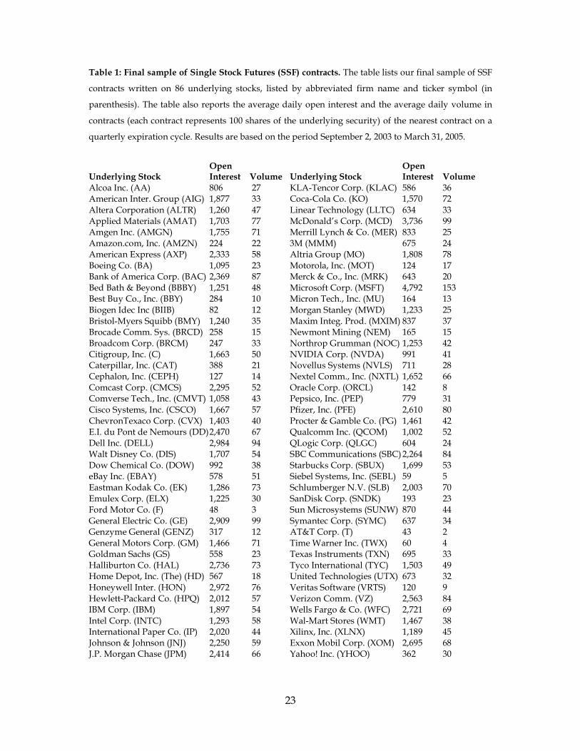
Table 1 lists the final sample of SSF contracts and provides the average daily

trading volume and average open interest of the nearby quarterly contract. While

clearly some contracts are less frequently traded than others, we note that the

arbitrage relation between the futures and underlying stock ensures that all contracts

have intraday bid-ask spreads which remain very narrow. 9 At expiration, open

contracts are settled by physical delivery.

8 When a contract is rolled over into the next nearby contract, a cost arises from the price difference

between the two contracts. This difference largely reflects the gap in the time value implicit in the contracts, but may also reflect differences due to the term structure of interest rates and/or trading patterns in SSFs. Because of these small differences, in practice, market participants may decide it is optimal to roll-over contracts prior to the expiration date. Nueberger (1999) and Bernhardt, Davies, and Spicer (2006) explore the optimal timing of this roll-over decision. While a proper analysis of these costs is beyond the scope of this paper, anecdotal evidence suggests that these roll-over costs are extremely small relative to the errors linked with the choice of hedging asset (the focus of this paper). 9 As anecdotal evidence of how relatively new SSF markets can have narrow spreads, the Futures Industry Magazine reports that on the Spanish futures exchange MEFF, “Underlying shares in the cash market, which are generally priced between 10 euro and 25 euro, trade with bid-ask spreads of 0.01 euro to 0.02 euro. The market for single stock futures are seeing bid-ask spreads of only 0.02 euro to 0.03 euro.” (“Spain’s MEFF Scores Solid Success”, Joshua Levitt, Futures Industry Magazine, Dec. 2001).

15

The criteria for the spot stocks included in our sample are that they must: i) not

have corresponding derivatives – either SSF or options;10 ii) be US-based firms; iii) be

listed on a U.S.-based stock exchange before September 2, 2003; and iv) have

matching characteristic data available. From the set of stocks satisfying these four

criteria, we select the largest 350 stocks based on market capitalization on December

31, 2003. For the spot stocks and the firms underlying the SSF contracts, we collect

matching characteristics (industry, beta, market capitalization, and price to book

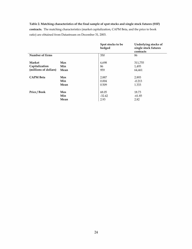
ratio) from Datastream. Table 2 provides summary statistics of the sample. Notice

that the firms underlying the SSF contracts are much larger, in general, than the

sample of spot stocks. Our restriction that spot stocks have no exchange-traded

derivatives written on them results in a sample of firms that is smaller and younger.

To the extent that these firms are more difficult to match, our results will provide a

conservative estimate of the true potential effectiveness of our hedging methods.

6 Results

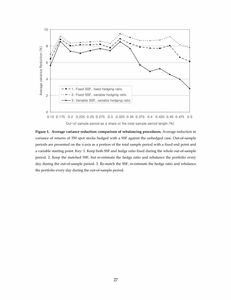
First, we examine the issue of which rebalancing procedure shows the best

hedging efficiency during the out-of-sample period. In Figure 1, the average variance

reductions from different rebalancing methods are depicted over different lengths of

out-of-sample period. Interestingly, our expectation that the most complicated

rebalancing method would show the best performance is not supported. All three

rebalancing methods are based on a hedge using a sole SSF matched by historical

correlation only. Even though rebalancing according to the time varying hedge ratio

performs better than the constant hedge ratio over the out-of-sample period,

changing the SSF used for hedging according to the updated historical return

correlation does not guarantee a better performance.

We have tested a total of 33 cases of hedging models – for example, hedging with

multiple SSF contracts, matching SSF contracts with different matching characteristic

sets, adding industrial classifications, and with market index futures. Even though

Figure 1 is based on the simplest hedging model, for most of the hedging models, the

second rebalancing procedure – re-estimating the hedge ratio and not re-selecting

the SSF – is still preferred. Hence, the following sections focus on the results

obtained from this second balancing method (that is, updating the hedge ratio but

using the same SSF for a given stock for the whole out of sample period).

10 This restriction ensures that hedging with the same futures asset as the underlying spot asset is not a possibility for any of the stocks in our sample.

16

When conducting an out-of-sample evaluation of hedging efficiency, it is of

interest to examine the sensitivity of the results to the portion of the total sample that

is retained as the out-of-sample period. To this end, we conduct all estimation

procedures for out-of-sample periods ranging from 15% to 50% of the total sample

period. Based on the results presented in Figure 1, we choose 32.5% of the total

sample (128 days) for the out-of-sample period, which also ties in with the loose

“two-thirds, one-third” rule commonly used in empirical analysis.

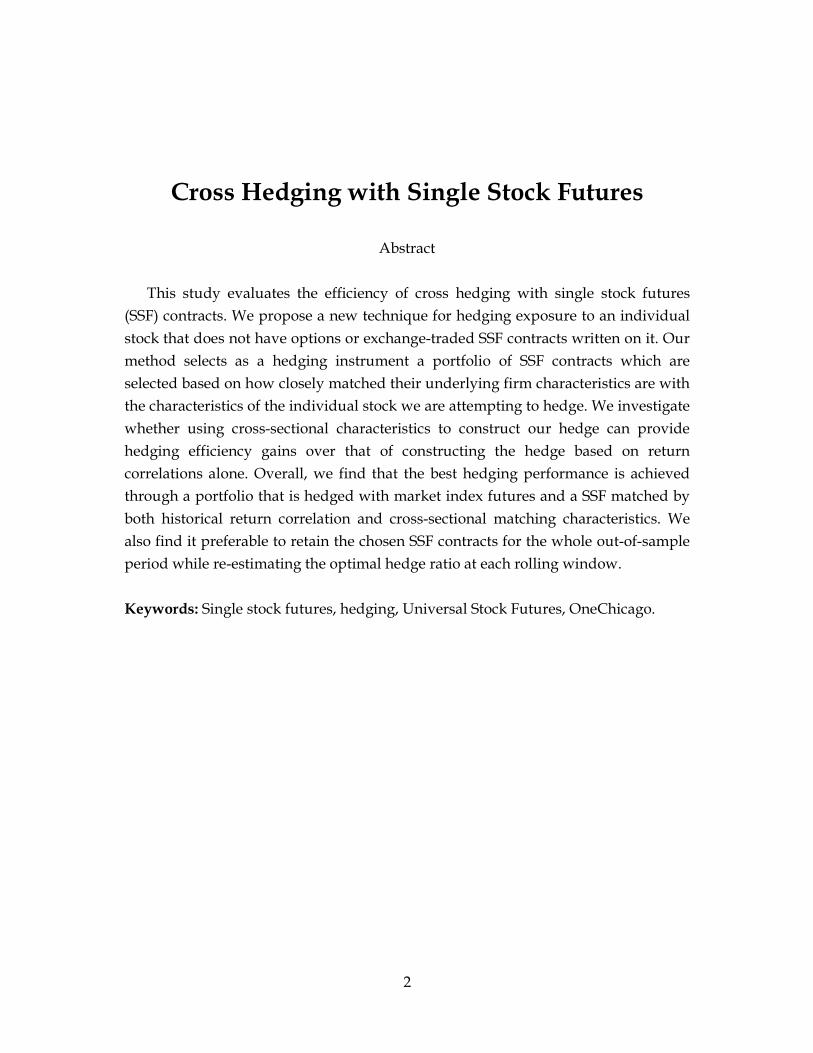
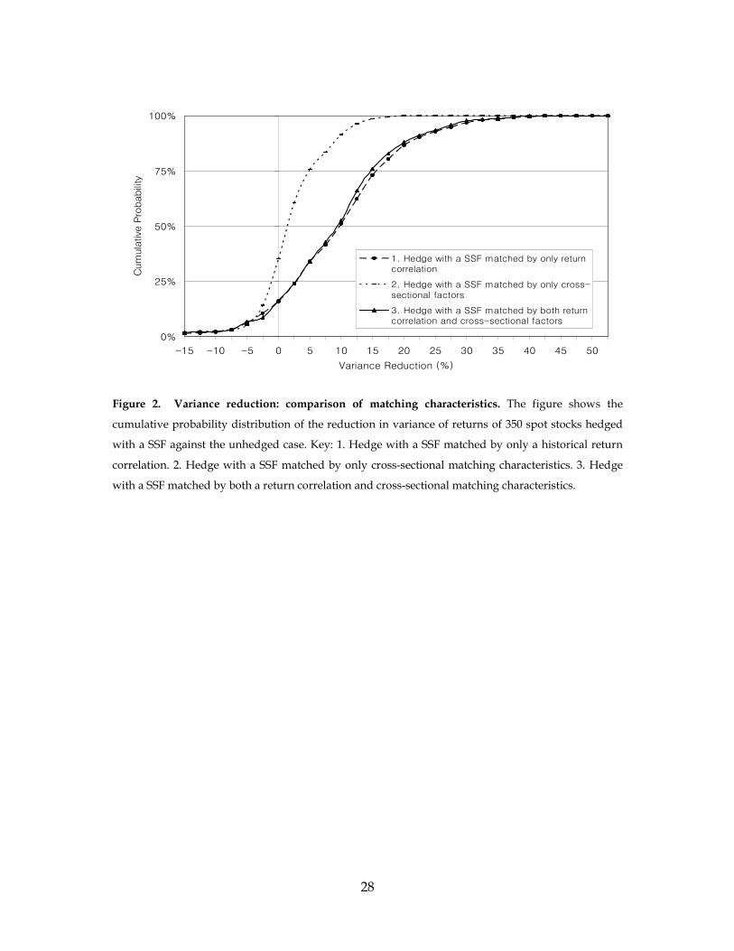
Matching characteristics: In figure 2, we examine the effect of three different

matching characteristics on the choice of optimal hedging asset. The first one consists

of the historical return correlation only while the second consists of three cross-

sectional matching characteristics (CAPM beta, market capitalization and price to

book ratio). Both the historical correlation and the cross-sectional matching

characteristics are combined in the last set. Note that in this cumulative probability

distribution diagram we prefer the line to be further to the lower right. Here, we

find that historical correlation is very important. For all three hedging models, the

variance of the hedged portfolio returns is reduced for about 75% of the spot stocks.

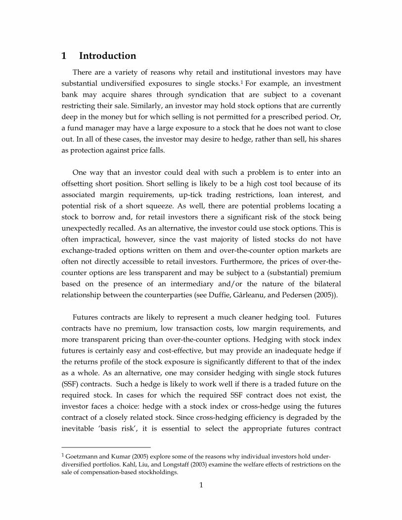
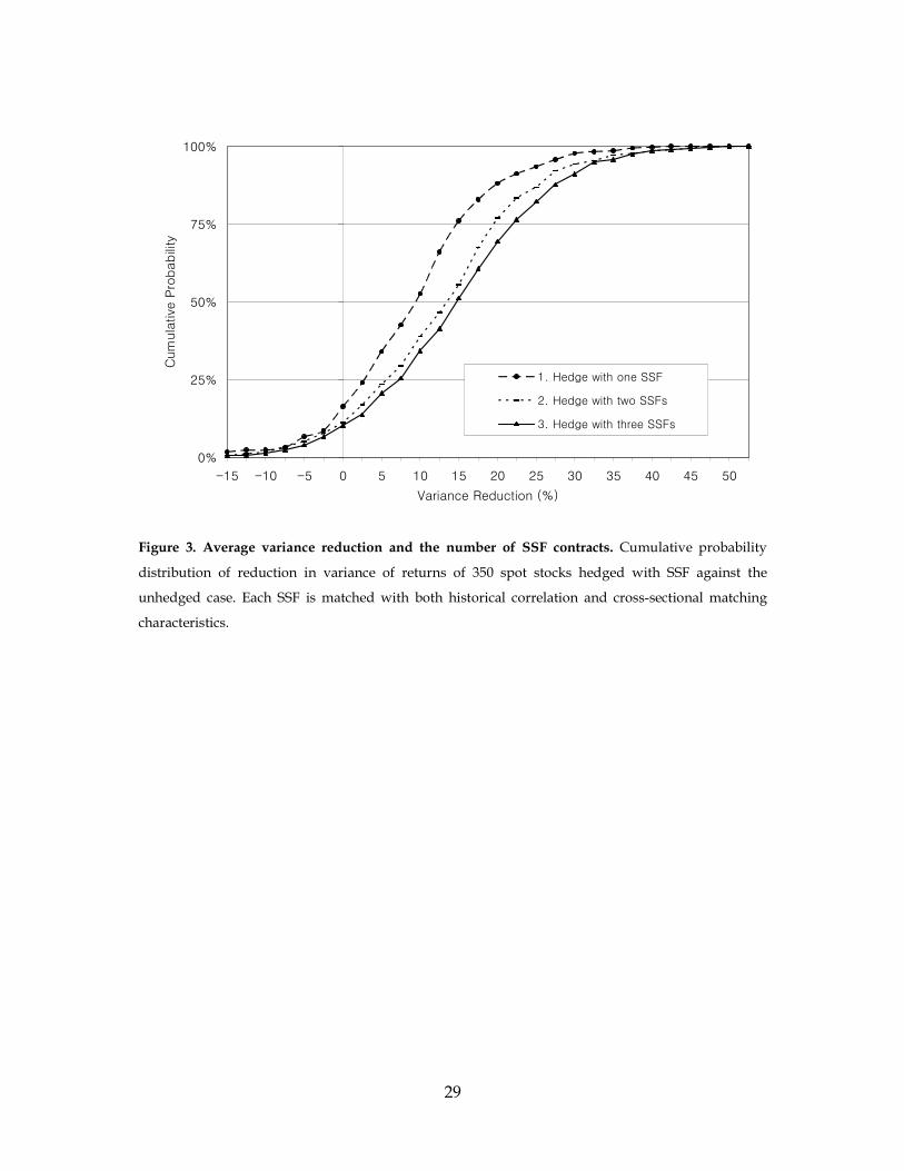
Multiple SSF contracts: If there are benefits from diversification, hedging with

multiple SSF contracts may improve hedging efficiency. In Figure 3, the variance

reduction from hedging with multiple SSF contracts is compared with that of

hedging with only one SSF for each stock. For hedging with three SSF contracts, half

of the spot stocks show at least a 15% variance reduction and 297 stocks (80%) show

a better performance than that of hedging with a single SSF.

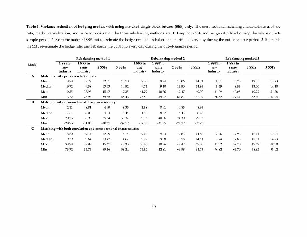
Table 3 summarizes the average variance reduction across the sample of 350

stocks. We find that the best approach is to use three SSF contracts selected on the

basis of both return correlation and firm characteristics, to adjust the hedge ratio

throughout the sample, and to fix the SSF’s employed (rebalancing method 2). In a

few cases, the median is much larger the mean, indicating that there are a few large

negative outliers. Such situations arise when the spot stock’s price collapsed or rose

spectacularly, but the hedging futures contract’s price did not; or vice versa. For

instance, during the out-of-sample period, three of the SSF contracts had very large

price falls: SanDisk fell about 30% on October 14, 2004; AMD fell about 25% on

November 1, 2004; and Biogen Idec fell almost 40% on February 28, 2005. Such

events are quite rare, but are bound to happen in a sample of this size.

17

Industry classification: Table 3 also examines whether matching SSF contracts

within the same industrial sectors as the spot stocks improves hedging efficiency.

Classifying by industry improves the results when only one SSF is used for each spot

stock hedged, but this improvement is less than that of moving from one to three SSF

contracts without concern for industry. The problem is that for the 86 SSFs available,

some industrial sectors contain no SSFs or very few. Comparing portfolios hedged

with industrial classification but limited to sole SSF hedging and the portfolio

hedged without industrial classification but unlimited as to the number of SSFs, the

latter shows better hedging efficiency in this context.

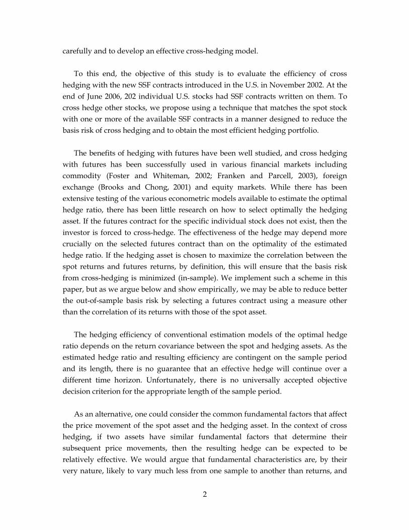
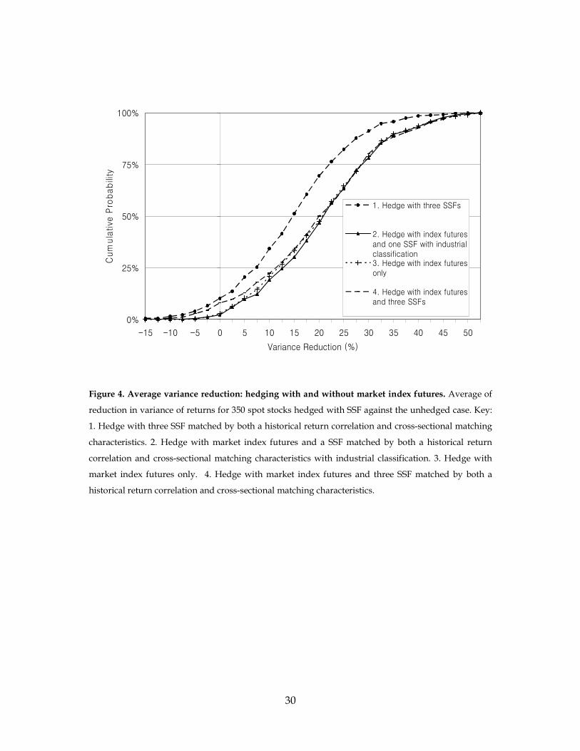
Market index futures: While hedging with SSF may reduce firm specific risk

because we hedge with a SSF similar to the spot asset, market risk will remain.

Hence, it is possible that hedging efficiency can be further improved by hedging

with market index futures. From Figure 4, it can be seen that controlling for market

risk as well does indeed improve the variance reduction. Adding market index

futures to the hedging model with three SSF, leads to an improvement in variance

reduction for half of the spot stocks from at least 14% to at least 21%.

Figure 4 illustrates that hedging with only market index futures shows a better

performance than hedging with both market index futures and three SSF contracts.

Since this may arise from noise caused by the use of so many hedging contracts, we

examine the hedging model with market index futures plus a single SSF matched by

return correlation, firm characteristics and industry sector. Hedging with index

futures and one SSF shows a slightly better performance than hedging with market

index futures alone (p-value = 0.07, one-sided paired t-test).

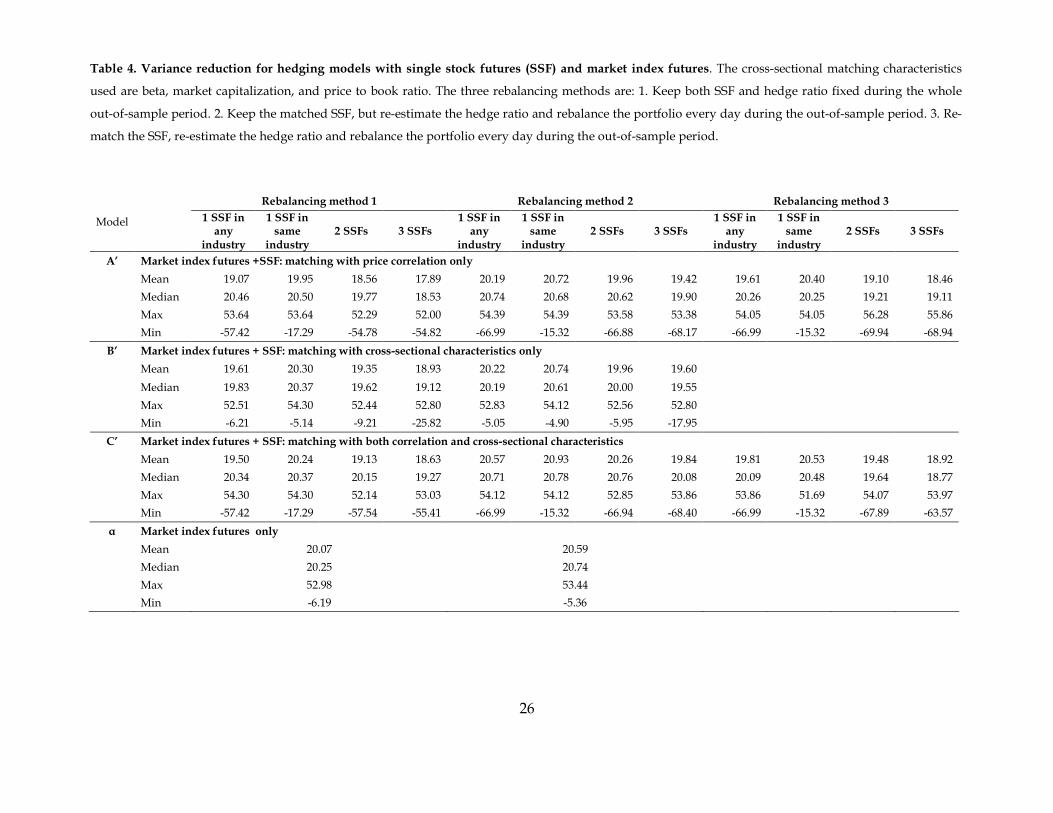
Table 4 provides the average reduction in variance across the sample of stocks for

the different hedging models. This table corresponds to Table 3, except that the

hedging is now done with market index futures as well as the SSF contracts. We find

that hedging with market index futures is effective, but that improvements can be

made by using both index futures and one SSF contract from the same industry as

the spot stock.

Optimal hedging model: To summarize, the best hedging performance is

achieved through a portfolio that is hedged with market index futures and a SSF

matched both by historical return correlation and by cross-sectional matching

characteristics, keeping the chosen SSF contract for the whole out-of-sample period

and using the optimal hedge ratio re-estimated for each rolling window. For the best

18

performing model, half of the spot stocks show at least a 21% reduction in variance

of returns and the best hedging model reduces the hedged portfolio variance for 94%

of spot stocks relative to no hedging. For interest, in terms of variance reduction,

Commercial Federal Corp, is the stock whose return movements can be hedged most

effectively – the variance of payoff is reduced 54%. Its matched SSF is Wells Fargo &

Co, which is in the same ‘Financials’ sector.

7 Conclusions

Investors holding positions in individual stocks may wish to hedge using futures

contracts, but it would be necessary for them to cross hedge (or to hedge with a stock

index) in the likely situation that there exists no futures contract on the spot stock(s)

that they hold. But the appropriate method for selecting the optimal futures contract

is not obvious. Thus, this study examines the use of sample matching techniques

together with fundamental firm characteristics for cross hedging with single stock

futures. Since individual stocks have very different characteristics from one another,

the efficiency of cross-hedging using futures whose underlying asset differs from the

spot stock may have been expected to be low.

We show that hedging efficiency can be improved by using industrial

classification to control for industry-specific effects or by using additional SSF

contracts to obtain additional diversification. Overall, matching the industry of the

SSF and spot stock is more important than the use of multiple SSF for hedging

efficiency. In addition, eliminating market risk is at least as important as eliminating

firm specific risk. Thus, hedging with market index futures as well improves

hedging effectiveness compared to hedging with only SSF contracts.

Our empirical results suggest that while single stock futures have much potential

for hedging firm-specific risk, they still have far to go before they become a viable

alternative to other traditional methods of hedging. Most of the SSF contracts

currently in existence are written on larger blue chip stocks. But these stocks already

have many viable hedging alternatives and are highly correlated with the market

index. Our results suggest that writing exchange-traded SSF contracts on smaller,

more diverse companies may be better suited for investor cross-hedging needs –

specifically, the firms underlying these contracts will be closer matches (in terms of

size and other firm characteristics) to the many small companies that lack other

suitable derivative products. By aiming to “complete the market” rather than

duplicate it, SSF exchanges may be better able to foster growth. It is worth noting

19

that regulators have been very nervous about allowing SSF contracts on smaller, less

liquid stocks because of market manipulation concerns. So, while contracts on

securities that do not have listed options might be more attractive, to-date they have

not been allowed.

To be fair, the results reported in this paper probably underestimate the true

effectiveness of our methods in practice. There are now more than twice as many

firms with SSF contracts written on them as used in this study. As the number of

available SSF contracts increases, hedgers will be able to more closely match firm

characteristics and thus further increase hedging efficiency.

20

References Anderson, R.W., J. Danthine, 1980. Hedging and Joint Production: Theory and Illustrations.

Journal of Finance 35(2), 487–498.

Anderson, R.W., J. Danthine, 1981. Cross Hedging. Journal of Political Economy 89(6),

1182–1196.

Ang, J.S., Y. Cheng, 2005a. Financial Innovations and Market Efficiency: The Case of Single

Stock Futures. Journal of Applied Finance 15(1), 38–51.

Ang, J.S., Y. Cheng, 2005b. Single stock futures: Listing selection and trading volume.

Finance Research Letters 2, 30–40.

Baillie, R.T., R.J. Myers, 1991. Bivariate GARCH Estimation of the Optimal Commodity

Futures Hedge. Journal of Applied Econometrics 6(2), 109–124.

Banz, R.W., 1981. The relationship between return and market value of common stocks.

Journal of Financial Economics 9(1), 3–18.

Bernhardt, D., R.J. Davies, J. Spicer, 2006. Long-term information, short-lived securities.

Journal of Futures Markets 26(5), 465–502.

Bertus, M., T.-H. Chu, S. Swidler, 2005. Quarterly versus serial expiration in pure cost of

carry markets: The case of single stock futures trading in the U.S., Working paper, Auburn

University.

Brooks, C., J. Chong, 2001. The Cross-Currency Hedging Performance of Implied versus

Statistical Forecasting Models. Journal of Futures Markets 21(11), 1043–1069.

Brooks, C., O.T. Henry, and G. Persand, 2002. The Effect of Asymmetries on Optimal

Hedge Ratios. Journal of Business 75(2), 333–352.

Cecchetti, S.G., R.E. Cumby, S. Figlewski, 1988. Estimation of the Optimal Futures Hedge.

Review of Economics and Statistics 70(4), 623–630.

Chau, F., P. Holmes, K. Paudyal, 2005. The impact of single stock futures on feedback

trading and the market dynamics of the cash market. Working paper, University of Durham.

DeMaskey, A.L., 1997. Single and Multiple Portfolio Cross-Hedging with Currency Futures.

Multinational Finance Journal 1(1), 23–46.

Duffie, D., N. Gârleanu, L.H. Pedersen, 2005. Over-the-counter markets. Econometrica

73(6), 1815–1847.

Dutt, H.R., I.L. Wein, 2003. On the Adequacy of Single Stock Futures Margining

Requirements. Journal of Futures Markets 23(10), 989–1002.

Ederington, L.H., 1979. The Hedging Performance of the New Futures Markets. Journal of

Finance 34(1), 157–170.

Fama, E., K. French, 1993. Common Risk Factors in the Returns on Stocks and Bonds.

Journal of Financial Economics 33, 3–56

Foster, F.D., C.H. Whiteman, 2002. Bayesian Cross Hedging: An Example from the Soybean

21

Market. Australian Journal of Management 27(2), 95–122.

Franken J.R.V., J.L. Parcell, 2003. Cash Ethanol Cross-Hedging Opportunities. Journal of

Agricultural and Applied Economics 35(3), 509–516.

Gatev, E.G., W.N. Goetzmann, K.G. Rouwnhorst, 2005. Pairs trading: performance of a

relative value arbitrage rule. Review of Financial Studies, forthcoming.

Goetzmann, W.N., A. Kumar, 2005. Why do individual investors hold under-diversified

portfolios? Working paper, Yale University.

Hung, M.W., C.F. Lee, L.C. So, 2003. Impact of foreign-listed single stock futures on the

domestic underlying stock markets. Applied Economics Letters 10(9), 567–574.

Johnson, P.M., 2005. Solving the mystery of stock futures. Financial Analysts Journal 61(3),

80–82.

Jones, T., R. Brooks, 2005. An analysis of single-stock futures trading in the U.S. Financial

Services Review 14(2), 85-95.

Jones, T., 2005. Individual investors, transaction fees, and growth in single-stock futures.

Working paper, Florida Gulf Coast University.

Kahl, M., J. Liu, F. Longstaff, 2003. Paper millionaires: How valuable is stock to a

stockholder who is restricted from selling it. Journal of Financial Economics 67(3), 385–410.

Knepper, Z.T, 2004. Examining the merits of dual regulation for single-stock futures: How

the divergent insider trading regimes for federal futures and securities markets demonstrate

the necessity for (and virtual inevitability of) Dual CFTC-SEC regulation for single-stock

futures. Pierce Law Review 3(1), 33–47.

Kroner, F.K., J. Sultan, 1993. Time-varying Distribution and Dynamic Hedging with Foreign

Currency Futures. Journal of Financial and Quantitative Analysis 28(4) 535–551.

Lascelles, D., 2002. Single Stock Futures, the Ultimate Derivative. CSFI Publications No. 52.

Lien, D., 2001a. A Note on Loss Aversion and Futures Hedging. Journal of Futures Markets

21(7), 681–692.

Lien, D., 2001b. Futures Hedging under Disappointment Aversion. Journal of Futures

Markets 21(11), 1029–1042.

Lien, D., Y.K. Tse, 2002. Some Recent Developments in Futures Hedging. Journal of

Economic Surveys 16(3), 357–396.

McKenzie, M.D., T.J. Brailsford, R.W. Faff, 2001. New Insight into the Impact of the

Introduction of Futures Trading on Stock Price Volatility. Journal of Futures Markets 21(3),

237–255.

Neuberger, A., 1999. Hedging long-term exposures with multiple short-term futures

contracts. Review of Financial Studies 12(3), 429–459.

Poomimars, P., J. Cadle, M. Thebald, 2003. Futures Hedging Using Dynamic Models of the

Variance/Covariance Structure. Journal of Futures Markets 23(3), 241–260.

Rosenberg, B., K. Reid, R. Lanstein, 1985. Persuasive evidence of market inefficiency.

22

Journal of Portfolio Management 11(3), 9–16.

Simons, H.L., 2002. Death, taxes & single stock futures. Futures, December, 34-36.

Tookes, H.E., 2004. Information, Trading and Product Market Interactions: Cross-Sectional

Implications of Insider Trading. Working paper, Yale School of Management.

23

Table 1: Final sample of Single Stock Futures (SSF) contracts. The table lists our final sample of SSF

contracts written on 86 underlying stocks, listed by abbreviated firm name and ticker symbol (in

parenthesis). The table also reports the average daily open interest and the average daily volume in

contracts (each contract represents 100 shares of the underlying security) of the nearest contract on a

quarterly expiration cycle. Results are based on the period September 2, 2003 to March 31, 2005.

Open Open Underlying Stock Interest Volume Underlying Stock Interest Volume

Alcoa Inc. (AA) 806 27 KLA-Tencor Corp. (KLAC) 586 36 American Inter. Group (AIG) 1,877 33 Coca-Cola Co. (KO) 1,570 72 Altera Corporation (ALTR) 1,260 47 Linear Technology (LLTC) 634 33 Applied Materials (AMAT) 1,703 77 McDonald’s Corp. (MCD) 3,736 99 Amgen Inc. (AMGN) 1,755 71 Merrill Lynch & Co. (MER) 833 25 Amazon.com, Inc. (AMZN) 224 22 3M (MMM) 675 24 American Express (AXP) 2,333 58 Altria Group (MO) 1,808 78 Boeing Co. (BA) 1,095 23 Motorola, Inc. (MOT) 124 17 Bank of America Corp. (BAC) 2,369 87 Merck & Co., Inc. (MRK) 643 20 Bed Bath & Beyond (BBBY) 1,251 48 Microsoft Corp. (MSFT) 4,792 153 Best Buy Co., Inc. (BBY) 284 10 Micron Tech., Inc. (MU) 164 13 Biogen Idec Inc (BIIB) 82 12 Morgan Stanley (MWD) 1,233 25 Bristol-Myers Squibb (BMY) 1,240 35 Maxim Integ. Prod. (MXIM) 837 37 Brocade Comm. Sys. (BRCD) 258 15 Newmont Mining (NEM) 165 15 Broadcom Corp. (BRCM) 247 33 Northrop Grumman (NOC) 1,253 42 Citigroup, Inc. (C) 1,663 50 NVIDIA Corp. (NVDA) 991 41 Caterpillar, Inc. (CAT) 388 21 Novellus Systems (NVLS) 711 28 Cephalon, Inc. (CEPH) 127 14 Nextel Comm., Inc. (NXTL) 1,652 66 Comcast Corp. (CMCS) 2,295 52 Oracle Corp. (ORCL) 142 8 Comverse Tech., Inc. (CMVT) 1,058 43 Pepsico, Inc. (PEP) 779 31 Cisco Systems, Inc. (CSCO) 1,667 57 Pfizer, Inc. (PFE) 2,610 80 ChevronTexaco Corp. (CVX) 1,403 40 Procter & Gamble Co. (PG) 1,461 42 E.I. du Pont de Nemours (DD) 2,470 67 Qualcomm Inc. (QCOM) 1,002 52 Dell Inc. (DELL) 2,984 94 QLogic Corp. (QLGC) 604 24 Walt Disney Co. (DIS) 1,707 54 SBC Communications (SBC) 2,264 84 Dow Chemical Co. (DOW) 992 38 Starbucks Corp. (SBUX) 1,699 53 eBay Inc. (EBAY) 578 51 Siebel Systems, Inc. (SEBL) 59 5 Eastman Kodak Co. (EK) 1,286 73 Schlumberger N.V. (SLB) 2,003 70 Emulex Corp. (ELX) 1,225 30 SanDisk Corp. (SNDK) 193 23 Ford Motor Co. (F) 48 3 Sun Microsystems (SUNW) 870 44 General Electric Co. (GE) 2,909 99 Symantec Corp. (SYMC) 637 34 Genzyme General (GENZ) 317 12 AT&T Corp. (T) 43 2 General Motors Corp. (GM) 1,466 71 Time Warner Inc. (TWX) 60 4 Goldman Sachs (GS) 558 23 Texas Instruments (TXN) 695 33 Halliburton Co. (HAL) 2,736 73 Tyco International (TYC) 1,503 49 Home Depot, Inc. (The) (HD) 567 18 United Technologies (UTX) 673 32 Honeywell Inter. (HON) 2,972 76 Veritas Software (VRTS) 120 9 Hewlett-Packard Co. (HPQ) 2,012 57 Verizon Comm. (VZ) 2,563 84 IBM Corp. (IBM) 1,897 54 Wells Fargo & Co. (WFC) 2,721 69 Intel Corp. (INTC) 1,293 58 Wal-Mart Stores (WMT) 1,467 38 International Paper Co. (IP) 2,020 44 Xilinx, Inc. (XLNX) 1,189 45 Johnson & Johnson (JNJ) 2,250 59 Exxon Mobil Corp. (XOM) 2,695 68 J.P. Morgan Chase (JPM) 2,414 66 Yahoo! Inc. (YHOO) 362 30

24

Table 2. Matching characteristics of the final sample of spot stocks and single stock futures (SSF)

contracts. The matching characteristics (market capitalization, CAPM Beta, and the price to book

ratio) are obtained from Datastream on December 31, 2003.

Spot stocks to be hedged

Underlying stocks of single stock futures contracts

Number of firms 350 86

Max 6,698 311,755 Min 86 1,495

Market Capitalization (millions of dollars) Mean 959 64,461

Max 2.887 2.893 Min 0.004 -0.213

CAPM Beta

Mean 0.509 1.333

Max 68.05 18.73 Min -32.42 -61.85

Price / Book

Mean 2.93 2.82

25

Table 3. Variance reduction of hedging models with using matched single stock futures (SSF) only. The cross-sectional matching characteristics used are

beta, market capitalization, and price to book ratio. The three rebalancing methods are: 1. Keep both SSF and hedge ratio fixed during the whole out-of-

sample period. 2. Keep the matched SSF, but re-estimate the hedge ratio and rebalance the portfolio every day during the out-of-sample period. 3. Re-match

the SSF, re-estimate the hedge ratio and rebalance the portfolio every day during the out-of-sample period.

Rebalancing method 1 Rebalancing method 2 Rebalancing method 3

Model 1 SSF in any

industry

1 SSF in same

industry 2 SSFs 3 SSFs

1 SSF in any

industry

1 SSF in same

industry 2 SSFs 3 SSFs

1 SSF in any

industry

1 SSF in same

industry 2 SSFs 3 SSFs

A Matching with price correlation only

Mean 8.88 8.79 12.51 13.70 9.46 9.24 13.06 14.21 8.51 8.75 12.35 13.73

Median 9.72 9.38 13.43 14.52 9.74 9.10 13.50 14.86 8.55 8.56 13.00 14.10

Max 40.35 38.98 45.47 47.35 41.79 40.86 47.47 49.30 41.79 40.05 49.22 51.38

Min -73.72 -73.93 -55.65 -55.43 -76.82 -35.27 -61.81 -62.19 -76.82 -27.41 -65.40 -62.94

B Matching with cross-sectional characteristics only

Mean 2.11 8.81 4.99 8.35 1.98 8.91 4.85 8.66

Median 1.61 8.02 4.84 8.44 1.56 8.07 4.45 8.05

Max 20.25 38.98 25.54 30.37 19.95 40.86 24.30 29.35

Min -28.95 -11.86 -20.61 -39.52 -27.16 -21.85 -21.17 -33.93

C Matching with both correlation and cross-sectional characteristics

Mean 8.30 9.14 12.39 14.14 9.00 9.33 12.85 14.48 7.76 7.96 12.11 13.74

Median 9.59 9.64 13.47 14.67 9.27 9.38 13.58 14.61 7.74 7.88 12.01 14.23

Max 38.98 38.98 45.47 47.35 40.86 40.86 47.47 49.30 42.32 39.20 47.47 49.30

Min -73.72 -34.76 -65.16 -58.24 -76.82 -22.81 -69.58 -64.73 -76.82 -66.70 -68.82 -58.02

26

Table 4. Variance reduction for hedging models with single stock futures (SSF) and market index futures. The cross-sectional matching characteristics

used are beta, market capitalization, and price to book ratio. The three rebalancing methods are: 1. Keep both SSF and hedge ratio fixed during the whole

out-of-sample period. 2. Keep the matched SSF, but re-estimate the hedge ratio and rebalance the portfolio every day during the out-of-sample period. 3. Re-

match the SSF, re-estimate the hedge ratio and rebalance the portfolio every day during the out-of-sample period.

Rebalancing method 1 Rebalancing method 2 Rebalancing method 3

Model 1 SSF in any

industry

1 SSF in same

industry 2 SSFs 3 SSFs

1 SSF in any

industry

1 SSF in same

industry 2 SSFs 3 SSFs

1 SSF in any

industry

1 SSF in same

industry 2 SSFs 3 SSFs

A’ Market index futures +SSF: matching with price correlation only

Mean 19.07 19.95 18.56 17.89 20.19 20.72 19.96 19.42 19.61 20.40 19.10 18.46

Median 20.46 20.50 19.77 18.53 20.74 20.68 20.62 19.90 20.26 20.25 19.21 19.11

Max 53.64 53.64 52.29 52.00 54.39 54.39 53.58 53.38 54.05 54.05 56.28 55.86

Min -57.42 -17.29 -54.78 -54.82 -66.99 -15.32 -66.88 -68.17 -66.99 -15.32 -69.94 -68.94

B’ Market index futures + SSF: matching with cross-sectional characteristics only

Mean 19.61 20.30 19.35 18.93 20.22 20.74 19.96 19.60

Median 19.83 20.37 19.62 19.12 20.19 20.61 20.00 19.55

Max 52.51 54.30 52.44 52.80 52.83 54.12 52.56 52.80

Min -6.21 -5.14 -9.21 -25.82 -5.05 -4.90 -5.95 -17.95

C’ Market index futures + SSF: matching with both correlation and cross-sectional characteristics

Mean 19.50 20.24 19.13 18.63 20.57 20.93 20.26 19.84 19.81 20.53 19.48 18.92

Median 20.34 20.37 20.15 19.27 20.71 20.78 20.76 20.08 20.09 20.48 19.64 18.77

Max 54.30 54.30 52.14 53.03 54.12 54.12 52.85 53.86 53.86 51.69 54.07 53.97

Min -57.42 -17.29 -57.54 -55.41 -66.99 -15.32 -66.94 -68.40 -66.99 -15.32 -67.89 -63.57

α Market index futures only

Mean 20.07 20.59

Median 20.25 20.74

Max 52.98 53.44

Min -6.19 -5.36

27

0

2

4

6

8

10

0.15 0.175 0.2 0.225 0.25 0.275 0.3 0.325 0.35 0.375 0.4 0.425 0.45 0.475 0.5

Out-of sample period as a share of the total sample period length (%)

Ave

rage v

ariance R

eduction (

%)

1. Fixed SSF, fixed hedging ratio

2. Fixed SSF, variable hedging ratio

3. Variable SSF, variable hedging ratio

Figure 1. Average variance reduction: comparison of rebalancing procedures. Average reduction in

variance of returns of 350 spot stocks hedged with a SSF against the unhedged case. Out-of-sample

periods are presented on the x-axis as a portion of the total sample period with a fixed end point and

a variable starting point. Key: 1. Keep both SSF and hedge ratio fixed during the whole out-of-sample

period. 2. Keep the matched SSF, but re-estimate the hedge ratio and rebalance the portfolio every

day during the out-of-sample period. 3. Re-match the SSF, re-estimate the hedge ratio and rebalance

the portfolio every day during the out-of-sample period.

28

0%

25%

50%

75%

100%

-15 -10 -5 0 5 10 15 20 25 30 35 40 45 50

Variance Reduction (%)

Cum

ula

tive

Pro

bability

1. Hedge with a SSF matched by only returncorrelation

2. Hedge with a SSF matched by only cross-sectional factors

3. Hedge with a SSF matched by both returncorrelation and cross-sectional factors

Figure 2. Variance reduction: comparison of matching characteristics. The figure shows the

cumulative probability distribution of the reduction in variance of returns of 350 spot stocks hedged

with a SSF against the unhedged case. Key: 1. Hedge with a SSF matched by only a historical return

correlation. 2. Hedge with a SSF matched by only cross-sectional matching characteristics. 3. Hedge

with a SSF matched by both a return correlation and cross-sectional matching characteristics.

29

0%

25%

50%

75%

100%

-15 -10 -5 0 5 10 15 20 25 30 35 40 45 50

Variance Reduction (%)

Cum

ula

tive

Pro

babili

ty

1. Hedge with one SSF

2. Hedge with two SSFs

3. Hedge with three SSFs

Figure 3. Average variance reduction and the number of SSF contracts. Cumulative probability

distribution of reduction in variance of returns of 350 spot stocks hedged with SSF against the

unhedged case. Each SSF is matched with both historical correlation and cross-sectional matching

characteristics.

30

0%

25%

50%

75%

100%

-15 -10 -5 0 5 10 15 20 25 30 35 40 45 50

Variance Reduction (%)

Cum

ula

tive

Pro

babili

ty

1. Hedge with three SSFs

2. Hedge with index futuresand one SSF with industrialclassification3. Hedge with index futuresonly

4. Hedge with index futuresand three SSFs

Figure 4. Average variance reduction: hedging with and without market index futures. Average of

reduction in variance of returns for 350 spot stocks hedged with SSF against the unhedged case. Key:

1. Hedge with three SSF matched by both a historical return correlation and cross-sectional matching

characteristics. 2. Hedge with market index futures and a SSF matched by both a historical return

correlation and cross-sectional matching characteristics with industrial classification. 3. Hedge with

market index futures only. 4. Hedge with market index futures and three SSF matched by both a

historical return correlation and cross-sectional matching characteristics.