1

Review of Crop Yield Forecasting Methods and Early Warning Systems

Bruno Basso1, Davide Cammarano, Elisabetta Carfagna

1Department of Geological Sciences

Michigan State University, USA

Abstract

The following review paper presents an overview of the current crop yield forecasting methods

and early warning systems for the global strategy to improve agricultural and rural statistics

across the globe. Different sections describing simulation models, remote sensing, yield gap

analysis, and methods to yield forecasting compose the manuscript.

1. Rationale

Sustainable land management for crop production is a hierarchy of systems operating in—

and interacting with—economic, ecological, social, and political components of the Earth. This

hierarchy ranges from a field managed by a single farmer to regional, national, and global scales

where policies and decisions influence crop production, resource use, economics, and

ecosystems at other levels. Because sustainability concepts must integrate these diverse issues,

agricultural researchers who wish to develop sustainable productive systems and policy makers

who attempt to influence agricultural production are confronted with many challenges. A

multiplicity of problems can prevent production systems from being sustainable; on the other

hand, with sufficient attention to indicators of sustainability, a number of practices and policies

could be implemented to accelerate progress. Indicators to quantify changes in crop production

systems over time at different hierarchical levels are needed for evaluating the sustainability of

different land management strategies. To develop and test sustainability concepts and yield

forecast methods globally, it requires the implementation of long-term crop and soil management

experiments that include measurements of crop yields, soil properties, biogeochemical fluxes,

and relevant socio-economic indicators. Long-term field experiments cannot be conducted with

sufficient detail in space and time to find the best land management practices suitable for

sustainable crop production. Crop and soil simulation models, when suitably tested in

reasonably diverse space and time, provide a critical tool for finding combinations of

management strategies to reach multiple goals required for sustainable crop production. The

models can help provide land managers and policy makers with a tool to extrapolate

experimental results from one location to others where there is a lack of response information.

Agricultural production is significantly affected by environmental factors. Weather

influences crop growth and development, causing large intra-seasonal yield variability. In

addition, spatial variability of soil properties, interacting with the weather, cause spatial yield

variability. Crop agronomic management (e.g. planting, fertilizer application, irrigation, tillage,

and so on) can be used to offset the loss in yield due to effects of weather. As a result, yield

forecasting represents an important tool for optimizing crop yield and to evaluate the crop-area

insurance contracts.

2

2. Crop Simulation Models

2.1. Background

Crop Simulation Models (CSM) are computerized representations of crop growth,

development and yield, simulated through mathematical equations as functions of soil

conditions, weather and management practices (Hogenboom et al., 2004). The strength of the

CSM is in their ability to extrapolate the temporal patterns of crop growth and yield beyond a

single experimental site. Crop Simulation Models (CSM) can be used to gain new scientific

knowledge of crop physiological processes or to evaluate the impact of agronomic practices on

farmers’ incomes and environments. Crop models are only an approximation of the real world

and many do not account for important factors such as weeds, diseases, insects, tillage and

phosphorus (Jones et al., 2001). Nevertheless, CSM have played important roles in the

interpretation of agronomic results, and their application as decision support systems for farmers

is increasing. Models range from simple to complex. The purpose a crop model is to be used

determines to a large extent the complexity of a model. Simple models are often used for yield

estimation across large land areas based on statistical information related to climate and

historical yields and include little detail about the soil-plant system. More complex mechanistic

models may provide detailed explanations of the soil-plant-atmosphere system and require a

large amount of input data, some of which may not be available. Models can be broadly

classified into two general groups: deterministic and stochastic. Deterministic models produce a

specific outcome for a given set of conditions, assuming all plants and soil within the simulation

space is uniform. Stochastic models produce outcomes that incorporate uncertainty associated

with the simulations. The uncertainty may arise because of spatial variability of soil properties,

weather conditions and other abiotic and biotic factors not accounted for in a deterministic

model. To overcome some of the problems with spatial soil variability, soil properties are

subdivided into small homogenous units and results using deterministic models are aggregated to

provide the entire field yield. Stochastic models are needed when the exactness of input

information is uncertain. The crop growth system in general is more stochastic than

deterministic because many parts of the agroecosystem are heterogeneous. However, to date,

crop models using a stochastic approach have not been developed to a level of usefulness in

decision making except in cases where year–to–year variations in weather are accounted for

using deterministic models. Deterministic crop models can be classified into three basic types:

statistical, mechanistic, and functional. The number of data inputs and the number and degree of

sophistication of functions help to contrast model types (Addiscott and Wagenett 1985).

Statistical Models

The first models used for large-scale yield simulations were statistical. Average yields from

large areas (counties or crop reporting districts) and for many years were regressed on time to

reveal a general trend in crop yields (Thompson, 1969; Gage and Safir 2011). The trend for the

past several decades has been usually been upward and accounts for technological advancements

3

in genetic and management s especially the increased use of fertilizers. Deviations from the

trend have been correlated with regionally averaged monthly weather data for each year.

Thompson (1986) used a statistical type model to determine the impact of climate change and

weather variability on corn production in five Midwestern states in the USA. He found pre-

season precipitation (September –June), June temperature, and temperature and rainfall in July

and August to be closely correlated with corn yield variations from the trend. Recently Gage and

Safir (2011) incorporated climate effect with the use of the Crop Stress Index (CSI) into the

regional yield trend. This approached significantly improved predictions of historical yields of

corn and soybean. Lobell et al. (2011, 2013) used statistical models to determine the effects of

increases in temperature on maize yield in USA concluding that temperature increase will play a

large role in yield decrease under climate change. In general, the results of statistical models

cannot be extrapolated to other space and time because of variation in soils, landscapes, and

weather not included in the population of information from whence the statistical information

was derived. Hence, the applicability of this type of crop-weather model to any areas and times

outside the area and time of the regression is limited. When simulating yield using statistical

models, the effects of changes in agricultural technology have to be subjectively extrapolated

into time when the mix of the technology is unknown for that period. Hence a principal problem

associated with statistical crop models is that the yield simulations may be made outside the

range of weather and technology information from which the model was developed. Statistical

models can provide many insights about past yields and historical influences and can be used to

inform the other kinds of models (Gage and Safir, 2011; Lobell et al., 2011)

Mechanistic Models

Mechanistic models attempt to use fundamental mechanisms of plant and soil processes to

simulate specific outcomes. Soon after computers became available for science, mechanistic

models were developed to simulate photosynthetic processes such as light interception, uptake of

carbon dioxide (CO2), respiration and production of biomass partitioning biomass into various

plant organs, and loss of CO2 during respiration. In the soil system, the mechanistic approach

was used to simulate the dynamics of water in the soil water due to infiltration, evaporation,

drainage, and root uptake. de Wit (1965) recommended to distinguish between two levels, the

system level and the next lower (explanatory) process level. Crop models typically consider the

processes of plant development, light interception, CO2 assimilation and respiration, and the

partitioning of biomass to plant organs and their growth. Including more detail at the process

level ultimately increases model complexity and calculation time. Developments in computer

science have progressively shortened calculation times and supported the consideration of more

explanatory detail. This and the increasing complexity of problems to be addressed have resulted

in the development of more complex models. Mechanistic models usually describe instantaneous

rates of plant processes that change rapidly over short time scales. For example, photosynthetic

and transpiration processes change rapidly during the day as the radiation and temperature

conditions change. A relatively large amount of input information is required to run such a

model. Uncertainty in some assumptions makes mechanistic model outcomes less certain and

4

often makes them less useful to those outside of the model development group. Mechanistic

models are seldom used for problem solving purposes; rather, they are often used for academic

purposes to gain a better understanding of specific processes and interactions.

Functional Models

Functional models use simplified approaches to simulate complex processes. In some cases,

mechanistic models can provide useful information that can be simplified into empirical

functions for models. For example, many functional models use daily solar radiation as the

amount of energy available for photosynthesis. The energy intercepted by the crop is

approximated using feedback information from the plant leaf area index to approximate the

biomass production using a simple concept of radiation use efficiency, e.g. the biomass produced

per unit of radiation intercepted. Although this type function is much simpler than the more

complicated ones, it usually produces reasonable results when compared to field measurements

(Ritchie, 1980). Evapotranspiration is also simulated using only daily weather inputs by

incorporating similar concepts to those used for biomass production simulation. In fact, the

functional Penman equation for simulating potential evapotranspiration was being used two

decades before computers were available for modeling and continues to be used, with some

modifications, in crop models.

Functional models usually use simplified equations and logic to partition the simulated

biomass into various organs in the plant, ultimately resulting in total biomass and economic

yield. Evapotranspiration is used in a water soil balance equation to approximate when deficits

or excesses in soil water or nutrients will impact potential biomass production and

evapotranspiration. Functional models practically always use capacity concepts to describe the

amount of water available to plants as compared to using instantaneous rate concepts from soil

physics. A lower and upper limit of water capacity is defined as inputs, and water inputs and

outflows in the soil provide the feedback to determine water availability to plants.

Functional models are usually run on daily time increments by using the daily inputs of

rainfall, temperature, radiation, and irrigation. The models use much less input data compared to

mechanistic models, making it more simple and useful for those not familiar with the biophysical

processes involved in the simulations. These type models, when properly tested can provide an

appropriate level of detail needed for assessing several issues affecting crop production.

Functional type models are now routinely used in decision support systems. Most of the

discussions in this paper hereafter will focus around the functional models that are used in

climate change assessment and to explore management issues related to crop production.

Advance in technology made possible the development of simple and complex CSM. The

main point to take into consideration is therefore the availability of information needed to run the

model. CSM need information of several aspects regarding crop management, soil, and

atmosphere (Table 1). There is a level of complexity in the input data as well, as they range

between hourly, daily, and weekly (Nix, 1984). However, CSM used for agrotechnology transfer

will preferentially run using daily input data. Hunt and Boote (1998) defined a Minimum Data

5

Set (MDS) for operating CSM that are used in agrotechnology transfer. MDS is defined as the

minimum amount of input data needed to run a CSM at a given site (Table 1).

The first step in acquiring input data for a CSM is to know the site where the model is to be

run, by gathering information such as the geographical coordinates (e.g. latitude, longitude, and

elevation). The required minimum weather data consists of daily incident solar radiation,

minimum and maximum temperature, and rainfall. If more details are available they can be used

to parameterize more complex functions within the CSM. For example, the MDS is generally

used to calculate potential evapotranspiration using the Priestly-Taylor method. If humidity and

wind speed are available then the FAO-56 approach can be used. The soil minimum information

requires soil type, texture, organic carbon, and bulk density. If soil hydraulic limits (e.g.

saturation, drain upper limit, and lower limit) and drainage coefficients are not available they can

be estimated with commonly used pedo-transfer functions. Management and initial conditions

can be obtained by farms’ surveys, expert knowledge, or published material.

Table 1. Minimum data set needed to operate a crop simulation model.

Input for CSM

1. Site description:

Latitude and longitude, elevation, average annual temperature

Slope and aspects of the site

2. Weather

Daily global soil radiation, daily maximum and minimum temperature, daily rainfall.

3. Soil

Soil type, soil depth (divided by n layers), soil texture, soil organic carbon, bulk density,

soil nitrogen, pH

4. Initial condition of the system

Previous crop, residues left on the soil (if any), initial soil water and soil nitrogen

5. Crop and field management

Cultivar name and type, planting date and type, row space, plants per square meter,

irrigation/nitrogen amount, method, dates of irrigation/fertilization, fertilizer type

3. Remote Sensing

Remote Sensing (RS) is defined as the science of acquiring information about an object

through the analysis of data obtained by a device that is not in contact with the object (Lillesand

and Keifer, 1994). Remotely sensed data can be of many forms, including variations in force

distribution, acoustic wave distribution or electromagnetic energy distributions. The data can be

obtained from a variety of platforms such as satellite, airplanes, unmanned vehicles, and

handheld radiometers. They may be gathered by different devices like sensors, film camera,

digital cameras, and video recorders. The instruments used for measuring electromagnetic

radiation are called sensors. Sensors are passive when they do not have their own source of

6

radiation and they are sensitive only to radiation from a natural origin; and active when they have

a built-in source of radiation.

Chlorophyll does not absorb all wavelengths of sunlight; it absorbs the blue (Blue) and red

(Red) wavelengths, while green (Green) light is reflected (Cambpell, 1996). The reflection of

visible radiation is mainly function of leaf pigments, whereas the Near-Infrared (NIR) is

reflected by the internal mesophyll structure of leaves. NIR radiation passes through the first

layer of the leaf (the palisade tissue); when it reaches the mesophyll and the internal leaf cavities

it is scattered both upwards (which is referred as reflected radiation) and downwards (transmitted

radiation) as shown in Figure 1 (Gausman et al., 1969). The behavior of the NIR reflectance is

also a function of leaf area index (LAI), cell turgor, leaf thickness, leaf internal air and water

content.

Figure 1. Section of a leaf and interactions between leaf structure and solar radiation (adapted from Campbell,

1996).

The relative decrease in reflectance is higher in the visible spectrum than in the NIR, because

of the effects of the transmittance of the NIR through the leaves and the absorption of red and

blue from the chlorophyll pigment. The visible light is absorbed or reflected by the first leaf

layers, while the NIR is transmitted downwards and reflected upwards partly from the soil and

partly during its passage through the canopy. These two reflected NIR wavelengths may be

detected by a sensor positioned above the crop. As a result of the above mechanism, healthy

crops will show high values of reflectance in the NIR and low values in the visible spectrum.

During senescence and in crops subjected to stress (e.g. disease, pests, nitrogen and water

shortages), the lower chlorophyll content allows for the expression of other leaf pigments such as

carotenes and xanthophyll, causing a broadening of the green reflectance peak at 550 nm and an

increase in visible light reflectance (Pinter et al., 2003). At the same time, there is a decrease in

the relative reflectance in the NIR, as a consequence of less absorption of visible light in the

leaves (Asner, 1998). The soil reflectance increases monotonically from the visible to the NIR

regions of the electromagnetic spectrum and its slope varies according to soil type (Huete, 1987).

In the visible region, leaf reflectance is lower than soil reflectance, whereas in the NIR leaf

reflectance is higher than soil reflectance (Figure 2).This behavior is useful for explaining the

utility of these reflectance measurements in agricultural applications and for the separation of

7

crops from soil (Bausch, 1993). The spectral reflectance of soil is a function of soil constituents

(such as soil organic matter, iron oxides), and soil roughness (such as particle and aggregate size)

(Rondeaux et al., 1996).

Figure 2.2. Percentage of visible and Near-Infrared (NIR) radiation reflected by wheat crop at Foggia (southern

Italy) with no nitrogen fertilisation (0 N) and with 90 kg N/ha as split application (90 N)

(Cammarano, 2010). Measurements are taken at the growth stage DC 30 (Pseudo-stem elongation,

Zadoks et al., 1974).

3.1. Vegetation indices

Vegetation indices (VIs) are mathematical combinations or ratios of mainly red, green and

infrared spectral bands; they are designed to find functional relationships between crop

characteristics and remote sensing observations (Wiegand et al., 1990). Vegetation indices are

strongly modulated by the interaction of solar radiation with crop photosynthesis and thus are

indicative of the dynamics of biophysical properties related to crop status. But at early crop

developmental stages, the effects of soil reflectance influence the values of some vegetation

indices for the detection of crop stress (Huete et al., 1985). Daughtry et al. (2000) classified VIs

into two categories: the intrinsic indices that include ratios of two or more bands in the visible

and NIR wavelengths, these indices are sensitive to soil background reflectance and are often

difficult to interpret at low Leaf Area Index (LAI) (Daughtry et al.,2000; Rondeaux et al., 1996).

The second category is the soil-line VIs that uses the information of a regression line using the

soil reflectance in the NIR-Red space to reduce the effect of the soil on canopy reflectance. On

the other hand, Baret and Guyot (1991) have classified VIs into two categories: Indices

characterized by “slope”: RVI; and indices characterized by “distance”. One of the first index

developed is the RVI is the Ratio Vegetation Index (Jordan, 1969) which is the ratio between

NIR and Red. The most commonly used index is the NDVI is the Normalized Difference

Vegetation Index (Rouse et al., 1973). A list of most common the VIs is presented in Table 2 and

an extensive list is discussed in Cammarano (2010).

0

0.1

0.2

0.3

0.4

0.5

0.6

0.7

0.8

350 450 550 650 750 850

Wavelenghts (nm)

Ref

lect

ance

(%

)

0 N

90 N

8

Table 2. List of the common Vegetation Indices (VIs), their mathematical formula, the scale at which they have been developed and

the parameter that they estimate (adapted from Cammarano, 2010).

Index Formula Reference Scale Parameter

NDVI (Normalized Difference Vegetation

Index)

Rouse et al., 1974 Canopy Biomass; Vegetation

Fraction

GNDVI (Green Normalized Difference

Vegetation Index)

Gitelson et al., 1996 Canopy Chlorophyll; Vegetation

Fraction

PRI (Photochemical Reflectance Index) Gamon et al., 1992 Canopy Photosynthesis efficiency/

RUE

NDRE (Normalized Difference Red Edge) Barnes et al., 2000 Canopy Chlorophyll/ Nitrogen

CCCI (Canopy Chlorophyll Content Index) Fitzgerald et al., 2006 Canopy N Status/ Chlorophyll

RVI (Ratio Vegetation Index)

Jordan, 1969 Leaf Biomass

EVI (Enhanced Vegetation Index)

Huete et al., 2002 Canopy/

Regional

Biomass/ Vegetation Cover

EVI 2 (Enhanced Vegetation Index 2)

Jiang et al., 2008 Canopy/

Regional

Biomass/ Vegetation Cover

VARIgreen (Visible Atmospherically

Resistant Index)

Gitelson et al., 2002 Canopy/

Regional

Vegetation Fraction/ LAI

VARI700 (Visible Atmospherically Resistant

Index; 700 nm)

Gitelson et al., 2002 Canopy/

Regional

Vegetation Fraction/ LAI

TVI (Triangular Vegetation Index) Brodge and Leblanc, 2000 Canopy Chlorophyll

MTVI 1(Modified Triangular Vegetation

Index 1) Haboudane et al., 2004 Canopy Chlorophyll

MTVI 2 (Modified Triangular Vegetation

Index 2)

Haboudane et al., 2004 Canopy Chlorophyll

MTCI

Dash and Curran, 2007 Canopy Chlorophyll

)Re(

)Re(

dNIR

dNIR

)(

)(

GreenNIR

GreenNIR

)531570(

)531570(

RR

RR

)720790(

)720790(

RR

RR

)(

)(

minmax

min

NDRENDRE

NDRENDRE

d

NIR

Re

)*2Re*1(

)Re(*5.2

LBlueCdCNIR

dNIR

1;5.72;61 LCC

1Re*5.7

6

Re*

dc

NIR

dNIRG

)(

*Re

cfG

Bluecd

)Re(

)Re(

BluedGreen

dGreen

)*3.1Re*3.2700(

)*7.0Re*7.1700(

BluedR

BluedR

)550670(200)550750(1205.0 RRRR

)550670(*5.2)550800(*2.1*2.1 RRRR

5.0)670*5800*6()1800*2(

)550670(*5.2)550800(*2.1*5.1

2

RRR

RRRR

25.68175.708

75.70875.735

RR

RR

9

CAR (Chlorophyll Absorption Reflectance) Kim et al., 1994 Canopy Chlorophyll

CARI (Chlorophyll Absorption Reflectance

Index)

Kim et al., 1994 Canopy Chlorophyll

MCARI (Modified Chlorophyll Absorption

Reflectance Index)

Daugthry et al.,

2000

Leaf/

Canopy

Chlorophyll/ LAI/ Soil

Reflectance

MCARI 1 Haboudane et al.,

2004

Canopy Chlorophyll/ LAI/ Soil

Reflectance

MCARI2 Haboudane et al.,

2004

Canopy Chlorophyll/ LAI/ Soil

Reflectance

TCARI (Transformed Chlorophyll Absorption

Reflectance Index)

Haboudane et al.,

2002

Canopy Chlorophyll/ LAI/ Soil

Reflectance

WDVI (Weighted Difference Vegetation Index) Clevers, 1989 Canopy LAI/ Biophysical

Parameters

PVI (Perpendicular Vegetation Index)

Richardson and

Wiegand, 1977

Canopy Canopy Biophysical

Parameters

SAVI (Soil-Adjusted Vegetation Index)

Huete et al., 1988 Canopy Canopy Biophysical

Parameters

TSAVI (Transformed Soil-Adjusted Vegetation

Index) Baret et al., 1989 Canopy Canopy Biophysical

Parameters

OSAVI (Optimized Soil-Adjusted Vegetation

Index) Rondeaux et al.,

1996

Canopy Canopy Biophysical

Parameters

MSAVI (Modified Soil-Adjusted Vegetation

Index) Qi et al., 1994 Canopy Canopy Biophysical

Parameters a L is a soil-adjustment factor and is set to be 0.5

b and c a and b are soil-line coefficients derived from the following equation: NIRsoil= a * REDsoil + b

d χis an adjustment factor for minimizing the soil background effects and is set to be 0.08

e L is a self-adjustment factor derived from the following equation: L= 1 – 2*a*NDVI*WDVI

1

670670*

2

a

bRa

)550*(550

150/)550700(

aRb

RRa

670

700*

1

670670*

2 R

R

a

bRa

670

700*)550700(*2.0670700

R

RRRRR

)550800(*3.1)670800(*5.2*2.1 RRRR

5.0680*5800*6)1800*2(

)550800(*3.1)670800(*5.2*5.1

2

RRR

RRRR

)670/700(*)550700(*2.0)700700(*3 RRRRRR

daNIR Re

)Re(1

1

2 bdaNIRa

LRR

RRLa

)670800(

)670800(*)1(

]670800[

)670800(

baRRa

bRaRa cb

)16.0Re(

)Re(*)16.01(

dNIR

dNIR

)670800(

)670800(*)1(

LRR

RRLe

10

4. Crop Yield Forecast

There are several methods of yield forecasting. The traditional method of yield forecasting is

the evaluation of crop status by experts. Observations and measurements are made throughout

the crop growing season, such as tiller number, spikelet number and their fertility percentage,

percentage of damage from pests and fungi, percentage of weeds infestation, and so on. From the

data obtained in this way yield can be forecasted using regression methods, or by the knowledge

from local expertizes. Other two methods used to forecast crop yield are the use of remote

sensing and crop simulation models. The objective of the yield forecast is to give a precise,

scientific sound and independent forecasts of crops’ yield as early as possible during the crops’

growing season by considering the effect of the weather and climate. The differences between

forecasts and final estimates are in the timing of the release. Forecasts are made before the entire

crop has been harvested whereas estimates are made after the crop has been harvested.

Indications are the result of applying a statistical estimator to the survey data and the resulting

point estimates are interpreted by commodity statisticians to make forecasts and estimates.

Historically, farmers have been always making “forecasts” in order to plan their agronomic

practices. For example, the planting window, the choice of a cultivar, the amount of fertilizer to

apply depend on the climate. If farmers know that the subsequent week there is a good chance

for rain, then they will rush into the field to sown their seeds. Forecasting crop yield means also

knowing or forecasting other important parameters. For example, quantifying the area planted at

the starting of the growing season and quantifying the area harvested.

Fig. 3. Diagram of yield forecast methods

4.1. Weather impact on crop yield variability: methods used to assess the direct and

indirect effects

4.1.1. Crop Yield Forecast using Statistical Models

Yield forecast using agrometeorological inputs into a statistical regression is rather common

and used in many yield forecasts research and programs (NASS, 2006; Lobell et al., 2009). In

general, a simple statistical model is build using a matrix with historic yield and several

agrometeorological parameters (e.g. temperature and rainfall). Then, a regression equation is

derived between yields as function of one or several agronometeorological parameters. The

NASS (2006) program uses a statistical model to forecast crop yield and production. They use

two methods to forecast yield, the former refer to the use sample-derived models for forecasting

yields and their component; the latter, is use models at state and regional levels. For example the

11

NASS (2006) system for corn forecast is based on the two levels described above. A corn

objective yield survey was first conducted in the 10 major corn-producing countries. They

conduct some detailed field surveys for determination of yield components which can be used for

the field-level yield forecast. While to obtain state/regional estimates an aggregation of the input

is done first and then a statistical model is used. The advantages of a statistical model is that the

calculation is easy, less time is required to run the model and the data requirements are limited.

However, they are limited in the information they can provide outside the range of values for

which the model is parameterized. Also the output of such models might not have any agronomic

meaning, while statistically are still correct. In addition, they do not take into consideration the

soil-plant-atmosphere continuum, which is important when dealing with regions having different

soil types. For example, the response of a crop to a given amount of rainfall on a sandy soil is

different than a crop on a clay soil. The timing of the water stress occurring during the growing

season is also important and often ignored. For example, a heat stress occurring at flowering will

reduce yield more than a heat stress happening during the vegetative phase. This is important for

correctly forecasting yield and for giving farmers important agronomic advices (e.g. timing and

amount of fertilizer, time of sowing, irrigation, and so on). There are efforts of include more

meaning into the statistical models in order to avoid some of the problems described. For

example, the inclusion of crop evapotranspiration, and/or the initial soil moisture content

(obtained through microwave sensing) as parameters of the model improve the predictability

power but leave the agronomic questions unanswered.

4.1.2. Crop Yield Forecast using Process-Based Models

Agroecosystems are complex entities where crop yield is the resultant of many interactions such

as soil, atmosphere, water, and socio-economic factors. CSMs are built with the aim to consider

the continuum soil-plant-atmosphere and its daily changes on the daily accumulation of biomass

and nitrogen. There are many CSM around the world, for example, Asseng et al. (2013) used

more 27 wheat models in their intercomparison. Not all the models are the same. Some are very

simple with no more than 7 parameters needed to describe a particular cultivar (Bondeau et al.,

2007), to other which take into account detailed processed like photosynthesis at leaf level and

therefore need many user-specified parameters. CSM have been extensively used to evaluate the

agronomic consequences from the inter-annual climate variability (Paz et al., 2007; Semenov and

Doblas-Reyes, 2007; Challinor and Wheeler, 2008). For example, CSM can capture the effects

of and timing of wet/dry cycles on crop growth; which can significantly help famers in planning

their agronomic management (Shin et al., 2009). Not all the CSM can be or will be used for

agrotechnology transfer; successful applications of a CSM to yield forecast is function of many

things but the most important is the amount of parameters needed to describe crop-soil-

atmosphere. A successful example of a CSM application is the yield prophet

(http://www.yieldprophet.com.au/yp/wfLogin.aspx) which is an on-line CSM designed to inform

farmers and consultants with real-time information about their crops, giving risk-assessment

information and monitoring decision support relevant to farm management. The system is

operated as a web interface for the Agricultural Production Systems Simulator (APSIM).

12

Another succesfful application of web-based simple interface crop simulation model is the

SALUS model as described by Basso et al., (2012, 2010) (www.salusmodel.net). The model is

designed to be used by farmers or extension specialists to quantify the impact of management,

soil and weather interaction on yield and environmental impact. The SALUS (System Approach

to Land Use Sustainability) model is an ongoing team effort started by Joe Ritchie at Michigan

State University in late nineties and currently carried on by Bruno Basso (Basso et al.2006;

Basso et al. 2010). SALUS is similar in detail to the DSSAT family of models but is designed to

simulate crop yield in rotation, soil, water and nutrient dynamic as function of management

strategies for multiple years (Fig. 1). SALUS accounts for the effects of rotations, planting dates,

plant populations, irrigation and fertilizer applications, and tillage practices. The models

simulates daily plant growth and soil dynamics processes on a daily time step during the growing

season and fallow periods. SALUS contains: i) crop growth modules; ii) soil organic matter and

nutrient cycling module and; iii) soil water balance and temperature module. The model

simulated the effects of soil-climate and management interaction on the water balance, soil

organic matter, nitrogen and phosphorus (P) dynamics, heat balance, plant growth and plant

development. i-Salus is also a web-based agronomic decision support system - named i-Salus - to

help farmers optimize their irrigation and nitrogen management practices over space and time. i-

Salus allows users to evaluate the best management strategy to improve yield and quality of the

crops, to increase economic net return and at the same time to reduce greenhouse gas emissions

and groundwater contamination from nitrate leaching. i-Salus is composed by two interfaces: a

simple interface and Web-GIS interface. SALUS with the simple interface is a user friendly

system s targets at farmers or extension specialists who can simulate the impact of different

management strategies on yield, and environmental impact. SALUS-WebGIS is a web-based

GIS integrated with Google Earth and Salus model to simulate in a spatial explicit manner the

effect of climate-soil-genotype-management interaction on crop yield and environmental impact.

Both systems are available at www.salusmodel.net

The difficulties of adopting CSM has usually been associated with the intensive data for

models’ parameterization. The need for calibration can be quite data extensive and not applicable

to some developing countries (Gommes, R, 1998). In fact, it has been argued that several

variables are needed to calibrate/evaluate the CSMs, concluding the usefulness of CSMs in some

“real” situation because of the impossibility of gathering inputs and calibration datasets.

However, a more critical look at the literature and the work done by other researcher points out

that the CSM can be run using “Minimum Data Set” (MDS) inputs (as discussed earlier).

Models, like the i-Salus example reported above, have shown to be easy to use by anyone but

still maintain its robustness in yield predictions. It has been pointed that another limitation of the

CSM is that they are “point-based” and inadequate to run at regional/national scale. However,

Bondeau et al. (2007) and Challinor et al. (2004) developed a simple CSM that can be run at

regional and national scale with less demands on inputs and calibration dataset.

13

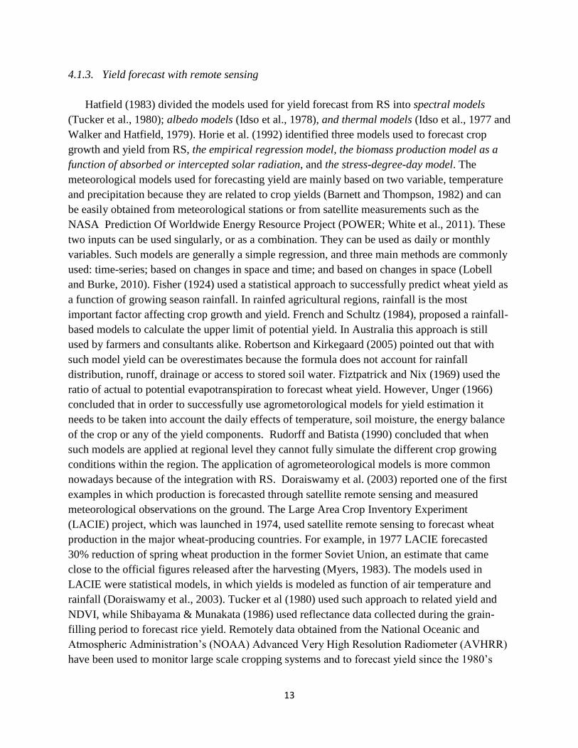
4.1.3. Yield forecast with remote sensing

Hatfield (1983) divided the models used for yield forecast from RS into spectral models

(Tucker et al., 1980); albedo models (Idso et al., 1978), and thermal models (Idso et al., 1977 and

Walker and Hatfield, 1979). Horie et al. (1992) identified three models used to forecast crop

growth and yield from RS, the empirical regression model, the biomass production model as a

function of absorbed or intercepted solar radiation, and the stress-degree-day model. The

meteorological models used for forecasting yield are mainly based on two variable, temperature

and precipitation because they are related to crop yields (Barnett and Thompson, 1982) and can

be easily obtained from meteorological stations or from satellite measurements such as the

NASA Prediction Of Worldwide Energy Resource Project (POWER; White et al., 2011). These

two inputs can be used singularly, or as a combination. They can be used as daily or monthly

variables. Such models are generally a simple regression, and three main methods are commonly

used: time-series; based on changes in space and time; and based on changes in space (Lobell

and Burke, 2010). Fisher (1924) used a statistical approach to successfully predict wheat yield as

a function of growing season rainfall. In rainfed agricultural regions, rainfall is the most

important factor affecting crop growth and yield. French and Schultz (1984), proposed a rainfall-

based models to calculate the upper limit of potential yield. In Australia this approach is still

used by farmers and consultants alike. Robertson and Kirkegaard (2005) pointed out that with

such model yield can be overestimates because the formula does not account for rainfall

distribution, runoff, drainage or access to stored soil water. Fiztpatrick and Nix (1969) used the

ratio of actual to potential evapotranspiration to forecast wheat yield. However, Unger (1966)

concluded that in order to successfully use agrometorological models for yield estimation it

needs to be taken into account the daily effects of temperature, soil moisture, the energy balance

of the crop or any of the yield components. Rudorff and Batista (1990) concluded that when

such models are applied at regional level they cannot fully simulate the different crop growing

conditions within the region. The application of agrometeorological models is more common

nowadays because of the integration with RS. Doraiswamy et al. (2003) reported one of the first

examples in which production is forecasted through satellite remote sensing and measured

meteorological observations on the ground. The Large Area Crop Inventory Experiment

(LACIE) project, which was launched in 1974, used satellite remote sensing to forecast wheat

production in the major wheat-producing countries. For example, in 1977 LACIE forecasted

30% reduction of spring wheat production in the former Soviet Union, an estimate that came

close to the official figures released after the harvesting (Myers, 1983). The models used in

LACIE were statistical models, in which yields is modeled as function of air temperature and

rainfall (Doraiswamy et al., 2003). Tucker et al (1980) used such approach to related yield and

NDVI, while Shibayama & Munakata (1986) used reflectance data collected during the grain-

filling period to forecast rice yield. Remotely data obtained from the National Oceanic and

Atmospheric Administration’s (NOAA) Advanced Very High Resolution Radiometer (AVHRR)

have been used to monitor large scale cropping systems and to forecast yield since the 1980’s

14

(Tucker et al., 1985). Benedetti and Rossini (1993) used the AVHRR satellite-derived NDVI

data for wheat forecast and monitoring in a region of Italy. They derived a simple linear

regression model for wheat yield estimate and forecast based on NDVI images during the wheat

grain filling period. They validated their results against official data and found good correlations

between the two. Doraiswamy et al. (2003) used the AVHRR NDVI data as proxy inputs to an

agro-meteorological model for the estimation of wheat yield at two different spatial resolutions

in North Dakota. Kogan et al. (2012) estimated winter wheat, sorghum and corn yields 3/4

months before harvest using the AVHRR data. The errors of yield estimated were 8%, 6%, and

3% for wheat, sorghum and corn, respectively. In Mediterranean African Countries, Maselli and

Rembold (2001) used the NDVI derived from the AVHRR platform to estimate cereal

production. While Meroni et al. (2013) using the SPOT platform (Satellite Pour l’Observation de

la Terre) and a statistical model quantified wheat yield in north Tunisia and concluded that where

crop conditions need to be quantified without ground measurements for calibration, the biomass

proxies are preferred. In Senegal, Rasmussen (1999) used the AVHRR data to estimate millet

yield, by using the NDVI integrated during the reproductive phase of millet development. He

also investigated if it was possible to reduce both the inter-annual and environmental variability

by taking into account areas of homogeneous production levels. Ray et al. (1999) used the Indian

Remote Sensing satellite (ISR) to estimate cotton yields at a district level using relationship

between actual evapotranspiration and non-irrigated cotton yield. The use of low resolution

satellite images, along with the high temporal frequency, their wide geographical coverage, and

their unitary low costs per area, means that these images are a good choice for yield estimation as

showed by many reported findings. In Western Australia Smith et al. (1995) used the AVHRR

satellite to estimate wheat yield over 70% of the wheat growing area of the state. For each

developmental stage the amount of variability explained by the NDVI-based model to predict

wheat yield. At stem elongation, the model built explained 45% of the variation in final yield;

56% of variance was explained around anthesis. However, after anthesis the amount of yield

explained was only 48%. Smith et al. (1995) concluded that the high correlation of the NDVI

taken during the growing season indicates the capability of correctly forecasting wheat yield well

ahead the end of the growing season.

Another platform that is commonly used is the National Aeronautics and Space

Administration’s (NASA) Moderate Resolution Imaging Spectroradiometer (MODIS), which has

been demonstrated to give better spectral and spatial resolution relative to the AVHRR

(Doraiswamy et al., 2001; Ren et al., 2008; Funk and Budde, 2009; Becker-Reshef et al., 2010).

AVHRR and MODIS have high frequency observations; but, both spatial resolutions are rather

coarse. For example, MODIS data are at a resolution of 250-m, 500-m, and 1000-m according to

the chosen product (Justice et al., 1998); while the AVHRR data have a spatial resolution of 1.1

km for local coverage and 4 km for global coverage (Kidwell, 1998). Bolton and Friedl (2013)

used satellite data from

15

MODIS to develop empirical models for maize and soybean yield forecast in the Central

United States. The EVI2 index (Table 2) showed better ability to predict maize yield than the

NDVI, and the use of crop phenology information from MODIS improved the model

predictability. Although MODIS has a low spatial resolution, the authors showed that MODIS

was still able to identify the agricultural areas without affecting model’s output compared to the

higher-spatial resolution crop-type maps developed by the USDA. Kogan et al. (2013) used

NDVI values from the MODIS, at 250 m spatial resolution for forecasting wheat yield in

Ukraine. In Kenya the MODIS was used to derive images for six sugarcane management zones,

over nine years, to estimate sugarcane yield based on each zone. Because of the zoning, the

different management strategies were taken into account using the temporal series of NDVI

which was normalized by a weighting method that includes sugarcane growth and the time-series

of the NDVI. The challenge is to estimate the yield in small-holder farmers where the fields are

often smaller that the spatial resolution of the MODIS used (250 m).

A platform with better spatial resolution (30 m) is the Landstat Thematic Mapper

(Hammond, 1975) and has been also used for yield forecast purposes (Rudorff and Batista, 1990;

Thenkabail et al., 1994). However, the Landsat temporal resolution is higher than the other two

which might be a problem if frequent observations are needed at sensitive crop growth stages.

Idso et al. (1980) used the LANDSAT reflectance data and the crop senescence to forecast grain

yield. This was achieved by using the concept of crop albedo variations through the growing

season (Idso et al., 1977, 1978). Wheat-field albedo always decreased from the time of heading

until the beginning of senescence. When crop is subjected to water stress senescence began to

appear earlier compared to well watered crops. Thus, Idso et al. (1980) used the senescence rates

and their correlation with grain yield to forecast production. Rudoff and Batista (1990) estimated

sugarcane in Brasil using remote sensing and an agrometeorological model based on a model

developed by Doorenbos and Kassam (1979) where yield is related to multiple regression

technique used to integrate the vegetation index from Landsat and the yield from the

agrometeorological model. Such estimations explained 69%, 54%, and 50% of the yield

variation in the 3 growing seasons analyzed. The authors also tested the accuracy of sugarcane

yield estimations using only the RS or the agrometeorological model only. The results were

poorer compared to the combinations of both (Rudorf and Batista, 1990).

Recent studies have used both higher spatial resolution data from Landsat with higher

temporal frequency data from MODIS or AVHRR (e.g., Genovese et al., 2001; Becker-Reshef et

al., 2010; Mkhabela et al., 2011). To generalize such models and make sure that they are reliable,

the use of physiological concepts has been introduced. One of the most frequent concepts used is

the Photosynthetically Active Radiation (PAR). The PAR is defined as the amount of light

available for photosynthesis that ranges between 400 and 700 nanometer (McKree, 1972).

Monteith (1977) proposed a simple model relating crop biomass, at any moment of the crop

growth, with the PAR accumulated; this model has been further validate by experimental

evidences (Shibles & Weber, 1966; Gallagher & Biscoe, 1978; Kumar and Monteith, 1982;

16

Sinclair & Horie, 1989; Daughtry et al.,1992; Gower et al., 1999). Bastiaanssen and Ali (2003)

combined the PAR model with a light use efficiency model developed by Field et al. (1995) and

the surface energy model of Bastiaanssen et al. (1998) to estimate crop growth and forecast crop

yield using the AVHRR data, for wheat, rice, sugarcane and cotton. The authors concluded that

even if AVHRR has a coarse resolution for field scale estimation it still provides useful yield

forecasts. The forecast of crop yield in sub-optimal growing conditions is harder to obtain.

However, the use of RS and physiological concepts such as the PAR can help to gain real-time

information of the crop growing conditions at any stage during the crop growing season

(Clevers, 1997). The use of PAR estimated from RS is used to predict sugar beet yield in Europe.

The parameters of model were not empirical estimates, but were derived using physiological

concepts. Another important crop parameter, the Leaf Area Index (LAI) has been linked with

remotely sensed data. LAI is defined as the total leaf area per unit of ground area (Watson,

1937). It is considered an important factor for describing several processes such as crop

evapotranspiration, photosynthesis, and yield (Price and Bausch, 1995). LAI is also a good

indicator of canopy ground cover; therefore, remote sensing has been used to link LAI

(Richardson & Wiegand. 1977: Tucker et al., 1979) or greenness (GR) (Rice et al.. 1980). The

Vls and greenness are linearly related to PAR absorption rate of crop canopies (Hatfield et

al.,1984; Asrar et al., 1985; Wiegand et al., 1979; Weigand & Richardson, 1990). Hence, crop-

absorbed PAR can be estimated from remotely sensed VI or greenness and PAR observed at

ground stations. This has been utilized for many crops to remotely estimate yields with

satisfactory results (Asrar et al., 1985: Wiegand et ai., 1989: Wiegand & Richardson, 1990). This

method, however, gives a potential crop yield rather than an actual yield: the constant radiation

conversion efficiency and constant harvest index are assumed. Radiation conversion efficiency is

affected by nitrogen deficiency (Sinclair & Horie, 1989) and water stress, while harvest index is

influenced by water or temperature stress during reproductive and grain-filling stages (Horie,

1987). Casanova et al. (1998) used VIs, and PAR to estimate LAI and biomass, and concluded

that estimation of biomass is more reliable of estimation of LAI. In fact at early growth stages

the low LAI and high soil reflectance makes it difficult to isolate the plant signal, affecting

relationships developed between spectral and canopy biophysical properties (Huete, 1988). Later

in the season, high values of LAI cause some VIs to lose sensitivity for detecting crop stress.

Carlson and Ripley (1997) found that when LAI values ranged between 3 and 6 NDVI become

ineffective. Daughtry et al. (2000) demonstrated that LAI is the main variable affecting VIs for

the estimation of leaf chlorophyll concentration.

The other model used in the integration of RS and yield forecast is based on the canopy

temperature measurements. The rationale behind this approach is that water stress causes

elevated plant temperatures which negatively affect plant photosynthesis and crop yield (Idso et

al., 1977; Idso, 1968). Idso et al. (1978) refer to this model as Stress Degree Day (SDD), where

canopy yield is inversely and linearly related to the accumulated SDD over a given period of

time during crop development. ldso et al. (1977) showed that the differences in canopy-air

temperatures at midday (SDD) were related to yield when cumulated over a period of time. This

17

model was used as a base for the forecast of crop yield and crop water status by RS. However,

the differences in temperatures between the leaf and the air is strongly influenced by the vapor

pressure deficit of the air and by soil moistures; therefore, the SDD application is somehow

limited to environments where the vapor pressure deficit is relatively constant (Horie, 1992).

Jackson et al. (1981) improved the SDD by creating the Crop Water Stress Index (CWSI) where

the vapor pressure deficit effects are taken into account. Gardner et al. (1981) proposed a

Temperature-Stress-Day (TSD) index, in which the temperature of the canopy and the field are

compared at an unknown stress level and for a fully-watered field with the same crop. Reginato

et al. (1978) found that for yield prediction the cumulative SDD for grain crops is calculated

from head appearance and awns to the end of plant growth. Idso et al. (1978) integrated the SDD

concept with the growing degree days (GDD) to better predict both grain yield and end of crop

growth. Yield forecast through RS and models has been made for several cropping systems. On

vineyards, the final yield was evaluated using high spatial resolution RS for the estimation of

canopy vigor and yield components (Hall and Wilson, 2013).

RS techniques have been extensively used in research for yield forecast but played a small

role in understanding the cause of spatial yield variability. Also, it has been argued that while RS

might not be suitable in developing countries because of their stratified agricultural systems and

very small farm sizes. However, this problem is hard to overcome in the near-future because of

the inability of RS to estimate yield in mixed agriculture. But, the increased availability of high-

spatial resolution RS at a reasonable cost make this technique a possible interesting alternative

for yield forecast. In fact, RS is often use in Early Warning Systems (next section) in developing

countries.

4.1.4. Yield Gap

The yield gap concept has been used for many years to define the difference between yield

potential and actual averages yield (van Ittersum et al., 2013). This is done in order to understand

the causes of yield gap and if the actual yields can be raised by better management practices

(Lobell et al., 2009). Crop yield potential (Yp) is defined as the crop yield obtained when a crop

is grown without limitations of water or nutrients, and in the absence of any pests, diseases and

weeds (Figure 4). In a given location crop yield potential is solely function of solar radiation, air

temperature and crop genetics feature (van Ittersum et al., 2003). In rain-fed environments, the

potential yield concept takes into account the constraints due to a water-limited environment

(Yw) in which crop growth (Figure 4). This means that along with factors affecting Yp, crop

yield is also dependent by soil characteristics (Lobell et al., 2009). The yield potential of a crop

can be experimentally determined in a field or obtained from well-managed farmer fields. This is

either costly or often hard to achieve (Lobell et al., 2005). Crop models have been used to

estimate Yp and Yw for specific fields, farms and regions (Lobell et al., 2009). In addition to

quantifying a potential yield, crop models have been used to understand the reasons for a yield

gap, the difference between actual and potential yield (Yp, Yw). Lobell (2013) added that in

assessing yield gap there is a spatial and temporal variability of agricultural land. Therefore,

18

when the yield gap is evaluated there is a mismatch in terms of reporting actual yield which are

reported at the level of administrative units; and the Yp that is generally quantified at field level

by using field trials, or point-based simulation models. However, the scale mismatch is often

ignored as well as the different management existing between a single farm and many farms

aggregated at an administrative level. Another example of using a CSM to find the yield

potential and the cause of lower yield has been described by Bachelor et al. (2002). The authors

used a crop model to attribute portions of a yield gap to disease, weeds and water stress effects.

Another important application of the RS is to forecast yield gaps. RS is an interesting

alternative for understanding the spatial and temporal variability of crop yield. RS has been

extensively used to estimate actual yield, but for the potential yield estimation several

approaches can be used. One approach consists in using Yp calculated in other ways and couples

them with RS estimations. But, Lobell (2013) concluded that such approach is not practical

because if Yp is known than actual yields are known as well and RS is not useful. The screening

of large areas over time is used to identify the highest yielding pixel and use it as a proxy for Yp

as demonstrated by Lobell et al. (2009). Lobell et al. (2002), and Bastiaanssen and Ali (2003)

used satellite data to derive the 95 percentile of the yield distribution. The main advantage of the

yield gap concept lies in its agronomic concept used to develop it, and the global approach for

evaluating simulated vs. observed Yp, Yw, and actual yields as described by Van Ittersum et al.

(2013). The main disadvantages are in the availability of global quality data, especially for crops

that are not common worldwide (e.g. cassava) or for developing nations where data are rather

sparse. However, as data are becoming widely available and several efforts to gather quality data

worldwide are underway this approach might become an appealing alternative to other simplistic

methods.

Figure 4. (a) Yields affected by defining, limiting and reducing factors for irrigated yield potential (Yp)

and rainfed yield (Yw). (b) Gap between average yields and 80% of Yp or Yw (from Van Ittersum et al.,

2013).

19

Figure 5. A diagram to illustrate the interaction between soil-plant-atmosphere as accounted in the SALUS model

(www.salusmodel.net)

5. Remote Sensing and Precision Agriculture

The past research efforts on remote sensing have provided a rich background of potential

application to site-specific management of agricultural crops. In spite of the extensive scientific

knowledge, there few examples of direct application of remote sensing techniques to precision

agriculture in the literature. The reasons are mainly due to the difficulty and expense of

acquisition of satellite images or aerial photography in timely fashion. With the progress in GPS

and sensor technology direct application of remote sensed data is increasing. Now an image can

be displayed on the computer screen with real-time position superimposed on it. This allows for

navigation in the field to predetermined points of interest on the photograph. Blackmer et al.,

(1995) proposed a system for N application to corn based on photometric sensors mounted on the

applicator machine. They showed that corn canopy reflectance changed with N rate within

hybrids, and the yield was correlated with the reflected light. Aerial photographs were used to

show areas across the field that did not have sufficient N. The machine reads canopy colors

directly and applies the appropriate N rate based on the canopy color of the control (well

fertilized) plots (Blackmer and Schepers, 1996; Schepers et al., 1996).

Management zones can be extracted using VIs maps and with the use of a GIS be viewed over a

remotely sensed image. The computer monitor displayed the image along with the current

position as the applicator machine moved on the field. When interfaced with variable rate sprayer

equipment, real time canopy sensors could supply site-specific application requirements

improving nutrient use efficiency and minimizing contamination of groundwater (Schepers and

Francis, 1998).

Indirect Applications

The most common indirect use of remote sensing images is as a base map on which other

information is layered in a GIS. Other indirect applications include use of remotely measured

soil and plant parameters to improve soil sampling strategies, remote sensed vegetation

parameters in crop simulation models, and use in understanding causes and location of crop

stress such as weeds, insect, and diseases.

20

Moran et al. (1997) in their excellent review on opportunities and limitations for image-based

remote sensing in precision agriculture, classify the information required for site specific

management in information on seasonally stable conditions, information on seasonally variable

conditions, and information to find the causes for yield spatial variability and to develop a

management strategy. The first class of information includes conditions that do not vary during

the season (soil properties) and only need to be determined at the beginning of the season.

Seasonally variable conditions, instead, are those that are dynamic within the season (soil

moisture, weeds or insect infestation, crop diseases) and thus need to be monitored throughout

the entire season for proper management. The third category is comprehensive of the previous

two to determine the causes of the variability. Remote sensing can be useful in all three types of

information required for a successful precision agriculture implementation. Muller and James

(1994) suggested a set of multi-temporal images to overcome the uncertainty in mapping soil

texture due to differences in soil moisture and soil roughness. Moran et al. (1997) also suggested

that multi-spectral images of bare soil could be used to map soil types across a field.

Crop growth and intercepted radiation

Remote sensing techniques have also been applied to monitor seasonally variable soil and crop

conditions. Knowledge of crop phenology is important for management strategies. Information

on the stage of the crop could be detected with seasonal shifts in the “red edge” (Railyan and

Korobov, 1993), bidirectional reflectance measurements (Zipoli and Grifoni, 1994), and temporal

analysis of NDVI (Boissard et al., 1993; Van Niel and McVicar 2004a). Moreover Wiegand et al.

(1991) consider them as a measure of vegetation density, LAI, biomass, photosynthetically active

biomass, green leaf density, photosynthesis rate, amount of photosynthetically active tissue and

photosynthetic size of canopies. Aparicio et al. (2000) using three VIs (NDVI; Simple Ratio;

Photochemical Reflectance Index) to estimate changes in biomass, green area and yield in durum

wheat. They results suggest that under adequate growing conditions, NDVI may be useful in the

later crop stage, as grain filling, where LAI values are around 2. SR, under rainfed condition,

correlated better with crop growth (total biomass or photosynthetic area) and grain yield than

NDVI. This fact is supported by the nature of relationship between these two indices and LAI.

SR and LAI show a linear relationship, compared to the exponential relationship between LAI

and NDVI. However the utility of both indices, as suggested by the authors, for predicting green

area and grain yield is limited to environments or crop stages in which the LAI values are < 3.

They found that in rainfed conditions, the VIs measured at any stage were positively correlated

(P < 0.05) with LAI and yield. Under irrigation, correlations were only significant during the

second half of the grain filling. The integration of either NDVI, SR, or PRI from heading to

maturity explained 52, 59 and 39% of the variability in yield within twenty-five genotypes in

rainfed conditions and 39, 28 and 26% under irrigation. Shanahan et al. (2001) use three

different kinds of VIs (NDVI, TSAVI, GNDVI) to asses canopy variation and its resultant impact

on corn (Zea mays L.) grain yield. Their results suggest that GNDVI values acquired during

grain filling were highly correlated with grain yield, correlations were 0.7 in 1997 and 0.92 in

21

1998. Moreover they found that normalizing GNDVI and grain yield variability, within

treatments of four hybrids and five N rates, improved the correlations in the two year of

experiment (1997; 1998). Correlation, however, increases with a net rate in 1997 from 0.7 to

0.82 rather than in 1998 (0.92 to 0.95). Therefore, the authors suggest that the use of GNDVI,

especially acquiring measurements during grain filling is useful to produce relative yield maps

that show the spatial variability in field, offering an alternative to use of combine yield monitor.

Raun et al. (2001) determined the capability of the prediction potential grain yield of winter

wheat (Triticum aestivum L.) using in-season spectral measurements collected between January

and March. NDVI was computed in January and March and the estimated yield was computed

using the sum of the two postdormancy NDVI measurements divided by the Cumulative

Growing Degree Days from the first to the second reading. Significant relationships were

observed between grain yield and estimated yield, with R2 = 0.50 and P > 0.0001 across two

years experiment and different (nine) locations. In some sites the estimation of potential grain

yield, made in March and measured grain yield made in mid-July differed due to some factors

that affected yield. The capability of VIs to estimate physiological parameters, as fAPAR, is

studied on other crops, faba bean (Vicia faba L.) and semileafless pea (Pisum sativum L.) that

grows under different water condition, as an experiment followed by Ridao et al. (1998) where

crops see above grew both under irrigated and rainfed conditions. They have computed several

indices (RVI, NDVI, SAVI2, TSAVI, RDVI, PVI) and linear, exponential and power

relationship between VI and fAPAR were constructed to assess fAPAR from VIs measurements.

During the pre-LAImax phase, in both species, all VIs correlated highly with fAPAR, however

R2

at this stage did not differ significantly between indices that consider soil line (SAVI2 and

TSAVI) and those that did not consider it (NDVI, RVI, RDVI). In post-LAImax phase the same

behaviour was observed. All VIs are affected by the hour of measurement at solar angles grater

than 45°. Authors conclude that simple indices as RVI and NDVI, can be used to accurately

assess canopy development in both crops, allowing good and fast estimation of fAPAR and LAI.

Nutrient Management

Appropriate management of nutrients is one of the main challenges of agriculture productions

and at the same environmental impact. Remote sensing is able to provide valuable diagnostic

methods that allow for the detection of nutrient deficiency and remedy it with the proper

application. Several studies have been carried out with the objective of using remote sensing and

vegetation indices to determine crop nutrient requirements (Schepers et al., 1992; Blackmer et

al., 1993; Blackmer et al., 1994; Blackmer et al., 1996a; Blackmer et al., 1994b; Blackmer and

Schepers 1996; Daughtry et al. (2000). Results from these studied concluded that remote sensing

imagery can be a better and quicker method compared to traditional method for managing

nitrogen efficiently. Bausch and Duke (1996) developed a N reflectance index (NRI) from green

and NIR reflectance of an irrigated corn crop. The NRI was highly correlated to with an N

sufficiency index calculated from SPAD chlorophyll meter data. Because the index is based on

plant canopy as opposed to the individual leaf measurements obtained with SPAD readings, it

22

has great potential for larger scale applications and direct input into a variable rate application of

fertilizer. Ma et al. (1996) studied the possibility to evaluate if canopy reflectance and greenness

can measure changes in Maize yield response to N fertility. They have derived NDVI at three

growing stage: preanthesis, anthesis and postanthesis. NDVI is well correlated with leaf area and

greenness. At preanthesis NDVI showed high correlation with field greenness. At anthesis

correlation coefficient of NDVI with the interaction between leaf area and chlorophyll content

was not significant with yield. Ma et al. (1996) summarized that reflectance measurements took

prior to anthesis predict grain yield and may provide in-season indications of N deficiency.

Gitelson et al. (1996) pointed out that in some conditions, as variation in leaf chlorophyll

concentration; GNDVI is more sensitive than NDVI. In particular is the green band, used in the

computing GNDVI that is more sensitive than the red band used in NDVI. This change occurs

when some biophysical parameters as LAI or leaf chlorophyll concentration reach moderate to

high values. Fertility levels, water stress and temperature can affect the rate of senescence during

maturation of crops. In particular Adamsen et al. (1999) used three different methods to measure

greenness during senescence on spring wheat (Triticum aestivum L.): digital camera, SPAD,

hand-held radiometer. They derived G/R (green to red) from digital camera, NDVI from an

hand-held radiometer and SPAD readings was obtained from randomly selected flag leaves. All

three methods showed the similar temporal behaviour. Relationship between G/R and NDVI

showed significant coefficient of determination and their relationship were described by a third

order polynomial equation (R2 = 0.96; P < 0.001). Relation is linear until G/R > 1, when canopy

approach to maturity (G/R < 1) NDVI is still sensitive to the continued decline in senescence

than did G/R. This fact suggests that the use of the visible band is limited in such conditions.

However authors found that G/R is more sensitive than SPAD measurements. Daughtry et al.

(2000) have studied the wavelengths sensitive to leaf chlorophyll concentration in Maize (Zea

mays L.). VIs as NIR/Red, NDVI, SAVI and OSAVI, have shown LAI as the main variable,

accounting for > 98% of the variation. Chlorophyll, LAI, and their interaction accounted for >

93% of the variation in indices that compute the green band. Background effect accounted for

less than 1% of the variation of each index, except for GNDVI, which was 2.5%. Serrano et al.,

(2000) studied the relationship between VIs and canopy variables (aboveground biomass, LAI

canopy chlorophyll A content and the fraction of intercepted photosynthetic active radiation

(fIPAR) for a wheat crop growing under different N supplies. The VIs-LAI relationships varied

among N treatments. The authors also showed that VI were robust indicators of fIPAR

independently of N treatments and phenology.

Li et al. (2001) studied spectral and agronomic responses to irrigation and N fertilization on

cotton (Gossypium hirsutum L.) to determine simple and cross correlation among cotton

reflectance, plant growth, N uptake, lint yield, site elevation, soil water and texture. NIR

reflectance was positively correlated with plant growth, N uptake. Red and middle-infrared

reflectance increased with site elevation. Li et al. (2001) found that soil in depression areas

contains more sand on the surface than on upslope areas. This behaviour modified reflectance

23

patterns. As a result, a dependence on sand content was shown by NDVI with higher values in

the depression areas and lower values in areas where the soil had more clay. In addition cotton

NIR reflectance, NDVI, soil water, N uptake and lint yield were significantly affected by

irrigation (P < 0.0012). The N treatment had no effect on spectral parameters, and interaction

between irrigation and N fertilizer was significant on NIR reflectance (P < 0.0027).

Wright (2003) investigated the spectral signatures of wheat under different N rates, and the

response to a midseason application at heading. VIs were computed (RVI, NDVI, DVI, GNDVI)

and spectral data were compared with pre-anthesis tissue samples and post-harvest grain quality.

The author found that imagery and tissue samples were significantly correlated with pre-anthesis

tissue samples and post-harvest grain quality. The second application of N at heading improved

protein only marginally. GNDVI was significantly correlated with nitrogen content of plants. VIs

used in the study, whether from satellite or aircraft correlated well with preseason N and plant

tissue analysis, but had lower correlation with protein. Osborne et al. (2002a; 2002b)

demonstrated that hyperspectral data in distinguishing difference in N and P at the leaf and

canopy level, but the relationship were not constant over all plant growth stages. Adams et al.

(2000) have detected Fe, Mn, Zn and Cu deficiency in soybean using hyperspectral reflectance

techniques and proposing a Yellowness Index (Adam et al. 1999) that evaluated leaf chlorosis

based on the shape of the reflectance spectrum between 570 nm and 670 nm.

Pest Management

Remote sensing has also shown great potential for detecting and identifying crop diseases

(Hatfield and Pinter, 1993) and weeds. Visible and NIR bands can be useful for detecting healthy

plants versus infected plants because diseased plant react with changes in LAI, or canopy

structure. Malthus and Madeira, 1993, using hyperspectral information in visible and NIR bands,

were able to detect changes in remotely sensed reflectance before disease symptoms were visible

to the human eye. Weed management represent an important agronomic practice to growers.

Weeds compete for water, nutrient, light and often reduce crop yield and quality. Decisions

concerning their control must be made early in the crop growth cycle. Inappropriate herbicide

application can also have the undesirable effect on the environment and a side effect to the crop.

With the advent of precision agriculture, there has been a chance from uniform application to the

adoption of herbicide-ready crop and to apply herbicide only when and where needed. This kind

of approach is economically efficient and environmentally sound but site-specific herbicide

management requires spatial information on the weeds. The discrimination between crops and

weeds is usually accomplished based on the differences in the visible/NIR spectral signatures of

crops and specific weeds (Gausman et al., 1981; Brown et al., 1994) or by acquiring images

when weed coloring is particularly distinctive. Richardson et al., (1985) demonstrated that

multispectral aerial video images could be used to distinguish uniform plot of Johnsongrass and

pigweed from sorghum, cotton and cantaloupe plots. Several other authors have utilized spectral

imagery to separate crops from weeds based on spectral signatures of species and bare soil

(Hanks and Beck, 1998) or based on the leaf shape determine by the machine vision technology

24

(Franz et al., 1995; Tian et al., 1999). Basso et al., 2004 used the handheld radiometer CropScan

to determine if a wheat field with various level of pappy (Papever Rhoeas) infestation could be

detected by the multispectral radiometer. The study showed that the reflectance in the Red and

NIR of the highly infested areas with pappy of the durum wheat field was significantly different

from the no infestations of lower levels of weed presence. Remote sensing can also be used to

determine herbicide injury to the crop for insurance purposes (Hickman et al., 1991; Donald,

1998a, Donald 1999b). To improve application efficiency of herbicides, Sudduth and Hummel

(1993) developed a portable NIR spectrophotometer for use in estimating soil organic matter as

part of the estimation procedure for the amount of herbicide to be sprayed. Several studies have

also been carried out using remote sensing for identifying and managing insects, mite and

nematode populations. Such studies have been able to demonstrate that remote sensing is able to

detect actual changes in plant pigments caused by pest presence, damages by pest and to identify

areas susceptible to infestation. Riedell and Blackmer (1999) infested wheat seedlings with

aphids and after 3 weeks they measured the reflectance properties of individual leaves. The

leaves of the infected plants had lower chlorophyll concentration and displayed significant

changes in reflectance spectra at certain wavelengths (500 to 525, 625 to 635 and 680 to 695

nm). This study in combination with others (Cook et al., 1999; Elliot et al., 1999; Willers et al.,

1999) suggests the potential usefulness of canopy spectra for identifying outbreaks in actual field

situations and to guide field scouts to specific areas for directed sampling. Site specific pesticide

application can reduce the impact of toxic chemicals on the environment by 40 percent (Dupont

et al., 2000).

Remote sensing and Crop Yield Estimation

Remote sensing can provide valuable information of yield assessment and show spatial variation

across the field. There are two approaches for yield estimation; the first is a direct method in

which predictions are derived directly from remote sensing measurements (Figure 6). The second

method is an indirect one, where remotely sensed data are incorporated into simulation model for

crop growth and development either as within season calibration checks of model output (LAI,

biomass) or in a feedback loop used to adjust model starting conditions (Maas, 1988). The

direct method for prediction yield using remote sensing can be based on reflectance or thermal-

based. Both methods have been applied with case of successes on various crops like corn,

soybean, wheat, alfalfa (Tucker et al, 1979; Tucker et al., 1981; Idso et al., 1977; Pinter et al.,

1981). Hatfield (1981) in his survey of 82 different varieties of wheat was not able to find a

consistent relationship between spectral indices and yield. Hatfield (1983b) coupled frequent

spectral reflectance and thermal observation in a more physiological method to predict yields in

wheat and sorghum. This method requires TIR daily measurements during grain filling period to

estimate crop stress. Shanahan et al., (2001) demonstrated that the time of corn pollination was

not a good growth stage to estimate yield because of the various that can cause tassel emergence

dates to vary. Yang et al., (2000) found similar results, concluding that images from images

taken at grain filling can provide good relationships between VIs and yield.

25

Reliability of imagery for use in yield estimation decreases as the time before harvest increases

because there are more opportunities for factors like various nature of stresses to influence yield.

Aase and Siddoway (1981) had cautioned that the relationships of spectral indices to yield were

dependent upon normal grain-filling conditions for the crop. Similar results were found by Basso

et al., 2004 (personal communication, unpublished data) where the NDVI images on a rainfed

durum wheat field showed different correlation to yield depending on the time of the image

selected. In this specific case, spatial variability of soil texture and soil water uptake by plants

affected by drought varied at anthesis presenting different scenarios from the one predicted by

the NDVI estimation.

6. Link between crop models and remote sensing for Yield Forecasting

The integration of RS and CSM for crop yield forecasting has been researched for almost three

decades, and is justified by the fact that RS can quantify crop status at any given time during the

growing season, while CSM can describe crop growth every day throughout the season (Maas,

1988). RS indirectly can provide measure for canopy state variables used by the CSM as well as

both spatial and temporal information about those variables which can then be used to adjust the

model simulation. Since the first satellite information became available to scientists, they have

developed algorithms to estimate canopy state variables, such as LAI, vegetation fraction and

fraction of APAR. One of the main integration procedures between RS and CSM focuses on

adjusting the LAI simulated with the crop models against the one estimated through RS. LAI it is

an important agronomic parameter because leaves are where water and CO2 are exchanged

between the plant and the atmosphere; in addition, the LAI is used to model crop

evapotranspiration, biomass accumulation and final yield (Strachan et al., 2005). Researchers

working on such integrations generally adopted three basic steps: (i) estimate canopy variables

with RS; (ii) run the CSM; (iii) use a proper integration method to adjust model runs. The first

step can affect the subsequent results of the integration because, if the crop variable is not

properly estimated, then adjusting the model with a biased variable will lead to a wrong model

evaluation. There are two ways of using RS for the estimation of canopy variables: through the

use of statistical/empirical relationships; and the Physical Reflectance Models that simulate the

interactions between solar beams (which is a definition of the concentrated stream of particle,

such as the light flux) and the various canopy components through the use of physical laws in

which the LAI can be entered as input obtained from the crop model (Dorigo et al., 2007).

The first methods consist of building relationships between the crop variables and RS or VIs,

such as the relationship between the Weighted Difference Vegetation Index (WDVI) and the LAI

(Clevers, 1989). Such models are built through the use of simple or multiple regressions,

stepwise multiple regressions, partial least square regressions (Hansen and Schjoerring, 2003;

Yoder and Pettigrew-Crosby, 1995). They are simple to build, easy to evaluate and do not

require a lot of computational effort. Successful application of this technique is reported in many

studies, such as the development of indices for the global estimation of crop parameters that are

sensitive to high biomass levels and less influenced by soil reflectance and atmospheric effects

26

(Jiang et al., 2008). The main limitation of the empirical/statistical methods is that, for every year

of measurement in the same field or for different sites, the relationships have to be recalibrated

because of changes in soil reflectance, canopy type and architecture. Notwithstanding, this

approach has been successfully used for the validation of crop models in a precision agriculture

context, because the simplicity of using NDVI maps and their empirical relationship with yield

help to characterise spatial patterns of crop growth variability, and the crop model will only be

validated in the areas defined by the RS map (Basso et al., 2001).

The second method involves the use of Physical Reflectance Models, which can simulate either

leaf reflectance or that of the overall canopy (Verhoef, 1984; Jacquemonod and Baret, 1990); for

practical purposes, physical models that simulate canopy reflectance are preferred because the

measured reflectance is collected in the field on an area base. Canopy reflectance models are

built on the radiative transfer theory that considers the canopy to be a turbid medium with leaves

that are small and distributed randomly. Canopy reflectance models are usually inverted to find

the best set of parameters that minimise the differences between the observed and simulated

canopy reflectance, and the methods used to find the best solution to the inversion are the

iterative technique, look-up tables and artificial neural networks (Moulin et al., 1998; Dorigo et

al., 2007). One problem of the inversion technique is that the solution does not produce a unique

value, because the variables affecting the overall canopy spectral signature have synergic effects

and compensation for this will affect the outcome (Fourty and Baret, 1997). For example, in their

review Baret and Guyot (1991) found that the modeled reflectance of sparse canopies with

horizontal leaves was similar to that of dense canopies with vertical leaves.

Farmers tend to use one or a few remote-sensed images for crop management, to retrieve canopy

variables with empirical or statistical methods, as this is more practical than the modeling

approach because it is simple and does not require extensive time, calculation or interpretation.

Moreover, canopy reflectance models require knowledge about the nature of the inputs and the

techniques required for the inversion, whereas in the statistical approach only the variable of

interest is taken into account. For example, taking remote observations before the application of

N fertilization and using a functional relationship between VIs and canopy N stress are more

practical for farmers and agronomists, who might not find the use of canopy reflectance models

attractive because of their greater complexity. It must be acknowledged, however, that canopy

reflectance models are an important tool for research purposes and for understanding the effects

of both crop architecture and soil reflectance on the overall canopy spectral signature. Therefore

the two methods might be considered complementary because, while scientists use physical

modeling approaches to either design new indices or understand the patterns of crop spectral

responses, agronomists can use the knowledge gained from models to derive empirical models

for better crop management (Cammarano, 2010). The other important step in the integration of

crop models and RS is the technique used to combine them. Maas (1988) analyzed four ways of

integration between RS and CSM, which are divided as follows:

27

Method 1. Evaluate driving variables: this technique is rather simple and uses RS information to

evaluate driving variables. Remote observations should be performed frequently during the

growing season, or at least frequently enough to perform interpolation techniques to obtain the

daily values of the RS estimated variable. Therefore, a limitation of this technique is that remote

observations are needed for each time-step of the simulation, which is not feasible either

practically or economically (Cammarano, 2010).

Method 2. Update model State Variables (SV): the daily values of the SV are simulated with the

CSM and, when RS data are available, the new values are simply updated into the CSM. For

example, many crop models use LAI to estimate biomass accumulation. The values of LAI and

biomass are simulated by the model and, when LAI estimated with RS is available. For this

technique, the accuracy of the variable updated is a function of the latest remote observation and,

because RS data carry some degree of error, the SV updated might present bias in its value that

cannot be minimized by more frequent remote observations; another limiting factor is that in the

model all the SV should be updated after RS acquisition (Cammarano, 2010).

Method 3. Re-initialize model State Variables (SV): This technique modifies the initial

condition of the SV in the crop model so that a new simulation will be in agreement with RS

observations. Indeed, different values of SV initial conditions in the crop model could lead to

different simulation scenarios. For example, when remote observations are available, the SV is

estimated from RS and there would likely be discrepancies between observed and simulated SV.

This effect is taken into account by considering the sum of the absolute errors between simulated

and observed values. This will lead to the creation of an error function and, through an iterative

numerical analysis technique (e.g. the secant method), it is possible to solve such a function and

find a new value of the SV; the new value will replace the old value required to initialize the

model. Re-initialization can be performed on one or more SV, leading to a uni– or multi-

dimensional solution of the problem. For example, this method has been used to derive new

values of LAI and used to calibrate the model (Maas, 1988). The re-initialisation procedure

provides good results in the estimation of biomass and final yield compared to previous

integration strategies, because RS is used to modify the SV in the model and at the same time

reduce the random error present in RS data. However, one limitation of this technique is in the

nature of the empirical relationship between RS and LAI; for example, NDVI values tend to

reach saturation levels at LAI values greater than 3 (Aparico et al., 2000), making NDVI

insensitive to changes in LAI after saturation in dense canopies. Also, such relationships may

have only local meaning and must be recalibrated for each new site.

Method 4. Re-parameterise model parameters: this technique is similar to the previous one with

the difference that the model parameters are modified after their estimation with RS observation.

The main difference is that typically a model has more parameters than SV and the minimising

procedure is more complicated, requiring more computational power. Indeed, while for re-

initialisation the error function is often two-dimensional, for the re-parameterisation it will

depend on the number of parameters involved. Therefore, the solution of the error function is

28

multi-dimensional and all the parameters should receive the same relative amount of change

(Cammarano, 2010). Since Maas (1988) published his ideas, many other conceptual models for

the integration of RS and CSM have been proposed, such as the reviewed classification for an

integration, which also identifies an “assimilation” technique (Moulin et al., 1998) in which RS

is directly used to re-parameterize or re-initialize the model. In this case, the daily crop

reflectance can be simulated with Physical Reflectance Models, and then the differences in

simulated and observed reflectance will be minimized by adjusting the initial conditions or the

model parameters of the CSM. An LAI simulated with CSM is first used as input in the canopy

reflectance model and then, once the errors between RS observed and simulated are minimized,

the new value of LAI can be adjusted in the CSM. But with this method, the number of

parameters that can be adjusted is a function of the frequency and the timing of RS observations.

Launay and Guerif (2005) used this assimilation procedure to spatially link the RS and CSM.

They found that in drought conditions CSM does not properly estimate LAI and its use in the

canopy reflectance model will not improve the robustness of such a method.

One of the key points for a successful integration of RS and CSM for in-season and between-

season crop management is that the whole system, defined as RS observation, crop simulation

and soil–crop–weather, is properly understood. One of the most challenging problems in the use

of both CSM and RS is trying to interpret, understand and evaluate the results in order to develop

the optimum agronomic management strategy that minimizes the observed variability in crop

production. Factors affecting crop growth, development and yield are well understood and

evidence of yield variability is normally provided but not explained (Cammarano, 2010). For

instance, final yield is a function of the complex temporal interaction of several variables such as

genotype, crop population, management, weather and stress (Bachelor et al., 2002). A CSM, to

some extent, takes into account the above effects, plus the temporal effects of stresses on crop

growth and development. However, the use of both model results and measured data to

understand the causes of particular spatial and temporal crop variability, and how it can be

managed from agronomic, economic and environmental point of view, is challenging. RS,

through the observation of the spatial patterns of VIs, allows the collection of information about

crop variability (Blackmer and White, 1998). Therefore, an integration strategy of RS and CSM

can be useful for in-season crop management and offers explanation of the causes of field

variability and how this can be managed. As a result, CSM should be used with the aim of

understanding crop temporal variability and RS images should be used to map the actual

distribution of crop spatial variability at a given time during the growing season. An example of

a spatial integration approach is described in Basso et al. (2001), in which a CROPGRO soybean

model (Boote et al., 1998) was used to validate three management areas across the field,

individuated with an NDVI map with a supervised classification technique. Soil properties and

average crop population were measured in each zone with targeted sampling and subsequently

used as inputs in the CROPGRO model. The model run was made only for those three zones

without calibration for the season, and the model simulated yield for these three zones with an

RMSE of 101 kg ha-1 with an average measured yield of 3000 kg ha-1. This technique has a

29

twofold advantage: it reduces the costs of using CSM for precision agriculture applications; and

model inputs and model parameterization are scale-independent because the scale is controlled

by the observed variation in the field, which is the scale where the model is applied (Bachelor et

al., 2002). The other approach to link RS and CSM is through the concept that the biomass

produced by a crop is function of the the amount of photosynthetically active solar radiation

(PAR) absorbed, along with the air temperature and soil conditions. The amount of absorbed

solar radiation if function of the incoming radiation and capability of crop’s interception of such

light. The latter is mainly function of the LAI. Such relationship LAI and PAR-intercepted has

been object of several reviews and studies (Asrar et al., 1984; Gallo et al., 1985; Tucker and

Sellers, 1986; Sellers, 1987; Baret and Guyot, 1991; Field et al., 1995; Frouin and Pinker, 1995;

Serrano et al., 2000; Goetz et al., 2005; Vina and Gitelson, 2005; Garbulsky et al., 2011; Wang et

al., 2013). The first steps that helped researchers to link RS and PAR was the equation developed

by Monteith in 1977 to quantify the PAR absorbed by the crop (fAPAR) (Monteith, 1977).

fAPAR depends mostly on LAI of the canopy and Monteith (1977) proposed an exponential

relation between LAI and fAPAR. fAPAR is quantified from RS because has been found a good

predictive ability by NDVI (Baret and Guyot, 1991). The close link between NDVI and fAPAR

has been confirmed in theoretical studies and later confirmed in experimental studies (Sellers,

1985; Sellers et al., 1997). The relationship between fAPAR and NDVI is justified because the

PAR intercepted and NDVI depend on LAI, leaf pigment concentrations, leaf angle orientation,

and soil reflectance features (Baret et al., 1989; Huete, 1985).

7. Early Warning Systems

7.1. Early Warning Systems history and definition

Humans have coped with natural disasters for centuries. However, the increase in human

population, the heavy anthropic modifications to the ecosystems and the effects of changing

climate make humans more susceptible to any disaster. Developing countries will suffer most

from any kind of disaster, like drought, floods, fires, bacterial and pests’ outbreaks and so on

(Deverux, 2009). Nowadays, scientific advance in many fields makes possible to use

technologies that can help to monitor several natural phenomena in a real-time both in time and

space. Therefore, an Early Warning System (EWS) is defined as an integrated system for

monitoring, data collection, analysis, and communicating to people in order to make early

decisions to protect peoples and the environment (Davies et al. 1991). The importance of a EWS

is because any degradation of the agricultural environment will cause famine, hunger, disease,

and death to millions of people. The FAO estimates that 1.02 billion people are hungry and

undernourished (FAO, 2013). For example, the UNEP (2002) estimated that in India more than

U.S.$10 billion is lost annually from anthropogenic land degradation, which in turns cause a loss

in productivity estimated around U.S.$2.4 billion (UNEP, 2002). Even in developed countries

agro-ecosystem degradation causes economic losses; for instance, in the USA soil erosion causes

30

losses for about $4 billion per year (Hrubovcak et al., 1995). To tackle this problem,

governments, United Nations (UN), Non-profit Organization (NGO), and academic institutions

have collaborated to implement systems to help reducing or preventing further environmental

degradation. There could be many reasons why the EWS is built, and that depends on the

objective of the system monitored. A EWS for agriculture will have a different structure than a

EWS that monitor human disease spread. Examples of integrated EWS are:

US Agency for International Development’s (USAID) Famine Early Warning System

(FEWS; USGS-EROS, 2010).

South African Development Cooperation’s (SADC) Food Security Programme (UNCCD

and Italian Cooperation, 1999).

Food and Agricultural Organization’s (FAO) Global Information & Early Warning

System (GIEWS) on Food and Agriculture (ISDR, 2009)

United Nation Environmental Programme’s (UNEP) Division of Early Warning and

Assessment (DEWA) (ISDR, 2010)

World Food Programme’s (WFP) Vulnerability Analysis and Mapping (VAM) (UNCCD

and Italian Cooperation, 1999)

Monitoring Agricultural Resources (MARS, 1988) of the European Union.

There are several commonalities among these systems, which are: (a) the way the work across

disciplines in collecting data and analyzing them; (b) the way the results are spread to the

scientific community, the general public, the stakeholders, and policy-makers; and (c) the way

the warning systems are implemented and how fast they can respond to a warning.

One of the first examples of EWS that were developed for use in forecasts was developed with

the aim of predicting the impact of El Nino on famine in Sub-Saharan Africa (Glantz, 1994).

But, the main cause of developing EWS was the response to food crisis in West Africa and the

Horn of Africa during the 70s and the 80s. For example, the GIEWS was developed in response

of the food crisis of the 70s. Nowadays it includes UN, donors, 117 national governments, 60

NGOs, and many research institutions (Rashid, 1997). The GIEWS that monitor crop status is

supported by the FAO Environment and Natural Resources Service with the help of the FAO’s

Africa Real Time Environmental Monitoring Information System (ARETMIS), and the support

of the experts in agrometorology, crops, and social science. In USA the severe drought in 1984-

1985 that caused more than a million deaths between Ethiopia and Sudan, made the Congress to

create the FEWS.

7.2. Early Warning Systems applications

Early Warning Introduction and ENSO

31

Examples of EWS application in agriculture need to take into account the constant crop

monitoring in a simple, timely and accurate manner. Provide forecasts and impact assessments at

national and regional levels of spatial and temporal variability of crop production and to a large

risk of famines. Most of the EWS use remotely sensed data for crop monitoring and early

screening for signs of drought, for flood, and for climate change impacts. Each EWS uses a

different satellite like the AVHRR, SPOT, and MODIS. Multi-years VIs images during the

growing season can help to identify years in which the crop had better or worse conditions from

an historical trend. Also, the seasonal patterns of NDVI in East Africa have been associated with

El Nino/Southern Oscillation (ENSO) index. Such index is derived from the atmospheric

pressure patterns in the Pacific sea, the temperature anomalies of the sea surface, and the

anomalies in the outgoing long-wave radiation. If the ENSO information can be translated into

practical advices and spread in a timely manner, farmers can adjust their management factors

(such as planting, fertilization, irrigation) in order to gain positive impacts on food security and

crop production. For example, in Mexico the economic gains of a EWS based on the ENSO has

been estimated of about US$ 10 million annually (Adams et al., 2003). The El Nino events are

known to cause issues to farmers in South East Asia as well. For example, an El Nino event in

Indonesia means delayed rainfall and less planted rice areas reducing the amount of rice

produced for that growing season, thus increasing the risk of annual rice deficits (Naylor et al.,

2007). Predictions of what could happen in the next 50 years suggested that farmers need to

adopt new management strategies to cope with reduced rainfall during the important crop stages.

The 1997-98 El Nino events, which was considered one of the strongest of the previous 50 years,

was related to vegetation patterns monitored by NDVI in Africa by Kogan (1998). Naylor et al.

(2007) concluded that increased investments in water storage, drought-tolerant crops, crop

diversification, and EWS can be adaptation strategies Indonesians’ farmers could adopt to offset

the negative effects of El Nino events in the future. Another part of the world where the Southern

Oscillation is known to affect crop yield is Australia. Rimmington and Nicholls (1993) discussed

how the wheat yields in Australia are correlated with values of the Southern Oscillation Index,

which affects growing season rainfall. Information of the Southern Oscillation Index is generally

available around the sowing date, and therefore can provide interesting yield forecasts.

Early Warning Drought and Yield

Drought events in Africa are important to forecast and prevent, because the lack of resources

means that a drought event will cause severe reduction of production and famine (Haile, 2005).

For example, 17 million people in East Africa are in drought-prone zones, and the recent

recurrence of drought makes these people at risk of food insecurity (Funk and Verdin, 2010).

Funk et al. (2003), using the FEWS system found that the agricultural areas of Ethiopia had a net

decline in growing season rainfall over the years, and that Ethiopia is facing an increase of food

shortages. This was caused by the anomaly warming in the Indian Ocean causing dryness in

Eastern Africa. Funk et al. (2008) linked this warming, to some extent, to anthropogenic

activities. Funk and Verdin (2010) argue that a combination of simple water and food balances,

32

still a useful tool for quantifying the evolution of the risk, coupled with spatial and temporal

analysis can be useful in providing information about early warnings. For example, the spatial

information of water per capita was used to derive information regarding the spatial patterns of

water availability per household (Funk et al., 2005). Then this information was used to derive 3

main zones of water security; the authors found a correlation between areas of low rainfall and

water security, but the urbanization of those areas compete for water used in agriculture. Two

points are interesting from Funk et al. (2005), firstly, that the vulnerable zones are increasing and

secondly, that there are some areas of water surplus. Ceccato et al. (2007) used remote sensing

for monitoring variations in rainfall and crop growth to help policy-makers in Sub-Saharan

countries to quantify the risk of desert locusts and malaria outbreaks. The monitoring of crop

yield, especially in rainfed areas like in many African countries, needs also to take into account

the temporal and spatial variability of rainfall. The AVHRR-NDVI product has also been used to

build a GIS system for detections of parasites in East Africa that can affect livestock and humans

alike (Malone, 1998). In Burkina Faso the cereal production is function of the amount and timing

of the growing season rainfall. The use of crop simulation model, Geographical Information

Systems (GIS), and RS has been used to build an early warning system for production anomalies

(Thornton et al., 1997). One limitation of the use of crop models in such locations is that the

weather station networks are very sparse and can present many gaps in data (Washington et al.,

2004), and that is why most researchers focus their attention on the use of RS, like the Satellite

Rainfall Estimation (RFE) to fill in gaps of missing rainfall. The droughts events are also

associated to the seat temperature anomalies and linked to anomalies in RS VIs. Using 8 years of

satellite data, Myemi et al. (1996) found correlations between the sea temperature of the Pacific

and NDVI anomalies that are considered anomalies in rainfall patterns in the arid and semi-arid

Africa, Australia and South America. Such results were also found in another study of Ayamba

and Eastman (1996). They used AVHRR NDVI for 4 years to study the trends of vegetation

greenness in Africa and the climate trends. They found a signal affecting Southern Africa, where

there is a significant relationship with the ENSO. In addition, in East Africa and the Sahel,

Ayamba and Eastman (1996) found that there is no correlation with ENSO in these areas and

concluded that the NDVI-ENSO is specific to certain regions of Africa. Another system for

drought monitoring is the seasonal rainfall forecasts, which is becoming widely available in

Africa as highlighted by Goddard et al. (2001). The FAO developed the Water Requirement

Satisfaction Index (WRSI; Frere and Popov, 1986) which estimated the effects of rainfall on crop

production in rainfed areas. The index uses decadal information of rainfall observations and soil

water holding capacity. The water demand is calculated using the potential evapotranspiration

approach of the FAO (Allen et al., 1998), while the supply is calculated from rainfall and soil

water. Spatial versions of the WRSI have been developed for Monazbique and for other African

countries using RS-NDVI and point WRSI to derive spatial maps for EWS (Rojas and Amade,

1998). In Algeria, the use of growing season rainfall has been used to empirically plan for

drought planning; but, El Mourid and Watts (1989) pointed out that in such area the approach is

not fully working because there is no correlation between autumn and spring rainfall, which is

33

the period for crops being more sensitive to drought. Monnik (2000) discuss of a EWS in South

Africa where an increase of droughts extremes has been experienced in the last 2 decades. In

South Africa farmers have the responsibility to plan for and survive droughts with minimum

intervention from the government, and therefore the EWS is vital to survival. For example in

South Africa, a EWS based on decile rainfall, the water satisfaction index, satellite NDVI, and

crop/pasture models is currently used.

The relationship of rainfall vs. seasonal NDVI has been also confirmed in other environments,

like the dry areas of the Negev Desert in Israel where this approach was used to quantify

vegetation cover (Schmidt and Karnieli, 2000). In fact, vegetation cover can be considered

another factor that might be implemented in EWS as a proxy for a desertification monitoring

system. Symeonakis and Drake (2004) estimated the vegetation cover and RUE using the NDVI

in Sub-Saharan Africa. In addition, they used the Meteosat data to derive rainfall, they also

calculated soil run-off and soil topography, in order to determine soil erosion. In this way they

can monitor in a real time the spatial and temporal trend of land degradation Symeonakis and

Drake (2004).

Early Warning and Climate Change

The IPCC reported that the temperature in Africa will increase 0.2 and 0.5°C per decade (IPCC,

2001). While future changes in rainfall amount is highly spatial variable. However, contrasting

results on the amount of temperature and rainfall changes are published (IPCC, 2001; Held et al.,

2005; Kamga et al., 2005; Huntingford et al., 2005). However, one thing it seems certain is that

the extreme events (e.g. drought, flood, heat spells) will be more frequent and this will seriously

impact crop production (Coppola and Giorgi 2005). For assessing future crop production and

implementing long term EWS is important to understand which tool can be used to assess the

impact of climate change on crop yield. Challinor et al. (2007) discussed several approaches

used, such as crop simulation models, empirical models, and yield transfer functions. One of the

most used empirical approaches like the FAO method (Doorenbos and Kassam 1979) is

relatively robust because based on conservative relationship between biomass and water use

(Hsiao and Bradford, 1983; and Hsiao,1993). However, such approach is well suited for large

scale applications because of its level of complexity. CSM can also be used at such large scale as

they have been modified to run at regional/national levels (Challinor et al., 2004; Bondeau et al.,

2017). Fischer et al. (2002) found that in 2080s projections of the GDP in Africa is lower under

climate change than in the relevant reference scenarios. A EWS therefore will help to understand

what are the measures that can adopted in response to such changes. For example, the adoption

of new cultivars, new management strategies (e.g. planting dates), new infrastructures (e.g. better

irrigation infrastructure) are some strategies to adopt in the next 10 years to offset negative

effects of climate (Reilly and Schimmelpfennig 1999). But, while planting dates can be easily

taken into account in crop models and therefore in impact assessment, new cultivars, or

infrastructure are harder to consider because of difficulties in parameterizing them causing an

increase in uncertainties (Southworth et al. 2002; Rosegrant and Cline 2003; Parry et al. 2004;

34

Challinor et al., 2007). Another interesting measure is expanding agriculture in new areas. In

East Europe, the re-use of abandoned farmland can help to offset some of the food decline due to

climate change (Alcantara et al., 2012). However, in Africa and South East Asia it is difficult to

create new cropland. The suitability of land for crop production is function of climate and soil, as

modeled by Ramankutty et al. (2002). In addition, in Africa the increase of food production are

not only related to agronomic practices but also to a series of socio-economic problems, such as

the growth of national economies, infrastructure improvements, and growth of income.

Unfortunately, yields in Africa are still amongst the lowest in the world; for instance, in sub-

Saharan regions the average rainfed cereal yields are 0.8 t ha-1

, which 50% below the lowest

yield for other regions of the world (Cooper 2004; FAOSTAT, 2013). Some of the remedies

famers are currently used to cope with changes in weather can become insufficient in the future

when extreme events will be more common. However, the EWS has to take into account the

social aspects of a particular area. An example on what a EWS should consider in case of climate

extremes is during the last Zimbabwe drought (Bird and Shepherd, 2003). The drought

significantly affected the availability and access to seed. Although there are systems such as the

Direct Seed Distribution (DSD), or Seeds and Tools (S&T), which have been created in to

extreme situations, several findings in Eastern and Southern Africa indicates that rarely the local

seed stocks are completely depleted, and alternative strategies may be more appropriate

(Sperling et al. 2004). In general, the problem is the access to the seed which is constrained by

many other factors. This example highlights the importance of a EWS that is cross-discipline,

from climate and crop scientists, agronomists, economists, and social scientists. So, building an

EWS for seed systems to climate change requires science (research into drought tolerant crops)

and policy, such as, government to optimize the seed system, law reforms for cross-border

movement of seed (Tripp 2001). In the subsequent years farmers face another important

challenge, to manage water supplies (irrigation or rainfall) more efficiently (Cooper 2004). Ellis-

Jones and Tenberg (2000) showed how collaborative research between scientists and farmers

helped developing efficient rainwater harvesting techniques, such as the improving of fallow

water storage through the use of agroforestry species (Kwesiga et al. 2005). But, even with such

techniques, some zones in Africa will no longer be suitable of certain crops. For example, Dietz

et al. (2004) showed that maize in the drier areas and groundnuts in the dryer zones of the Sahel

are at risk. Researchers acknowledge that African farmers have been successfully adapting to

changes in climate in the past (Boserup, 1965; Hill 1963). Reij and Waters-Bayer (2001)

discussed on how farmers have been adapting to changes in climate and what kind of technology

and management they have introduced to offset yield decline. This has been also found true in

many African regions (Haggleblade et al. 1989; Tiffen et al. 1994). However, the adaptation

capabilities are of little use for coping with extreme without a proper EWS in place.

8. Conclusion

The main conclusion of this review can be summarized as follows:

35

1. Statistical models are simple in their usage and less parameter-intensive, but they are

limited in the information they can provide outside the range of values for which the

model is parameterized. They do not take into consideration the soil-plant-atmosphere

continuum, the timing of the stresses occurring during the growing season, and do not

give farmers any important agronomic advices (e.g. timing and amount of fertilizer, time

of sowing, irrigation, and so on).

2. Crop simulation models vary greatly between them. Some of them are rather hard to use

and parameterize. The need for calibration can be quite data extensive and not applicable

to some developing countries. New models like SALUS have been developed to

overcome these limitation

3. RS techniques have been extensively used in research for yield forecast but might not be

suitable in developing countries because of their stratified agricultural systems and very

small farm sizes. However, this problem is hard to overcome in the near-future because

of the inability of RS to estimate yield in mixed agriculture. But, the increased

availability of high-spatial resolution RS at a reasonable cost make this technique a

possible interesting alternative for yield forecast. In fact, RS is often use in Early

Warning Systems in developing countries.

4. The integration of RS, yield gap and CSM represents an interesting alternative in crop

yield forecasting. RS can quantify crop status at any given time during the growing

season in a spatial context, while CSM can describe crop growth every day throughout

the season (Maas, 1988). RS indirectly can provide measure for canopy state variables

used by the CSM as well as both spatial and temporal information about those variables

which can then be used to adjust the model simulation. While the yield gap can provide

strong agronomic foundations of the yield potentials and the causes leading to the gap.

9. References

Adams, R.M., Houston, L.L., McCarl, B.A., Tiscareño L.M., Matus G.J., Weiher R.F., 2003. The

benefits to Mexican agriculture of an El Niño-southern oscillation (ENSO) early warning

system. Agricultural and Forest Meteorology 115, 183–194.

Acantara, C., Kuemmerle, T., Prishchepov, A.V., Radeloff, V.C., 2012. Mapping abandoned

agriculture with multi-temporal MODIS satellite data. Remote Sens. Environ. 124, 334–347.

Allen, R.G., Pereira, L.S., Raes, D., Smith, M., 1998. Crop evapotranspiration: guidelines for

computing crop water requirements. Food and Agriculture Organisation of the United

Nations, Rome, FAO Irrigation and Drainage Paper 56, 300 p.

36

Aparicio, N., Villegas, D., Casadesus, J., Araus, J.L., Royo, C., 2000. Spectral Vegetation

Indices as Nondestructive Tools for Determining Durum Wheat Yield. Agron. J. 92, 83-91.

Asseng, S., Ewert, F., Rosenzweig, C., Jones, J.W., Hatfield, J.L., Ruane, A.C., Boote, K.J.,

Thorburn, P.J., Rotter, R.P., Cammarano, D., Brisson, N., Basso, B., Martre, P., Aggarwal,

P.K., Angulo, C., Bertuzzi, P., Biernath, C., Challinor, A.J., Doltra, J., Gayler, S., Goldberg,

R., Grant, R., Heng, L., Hooker, J., Hunt, L.A., et al., 2013. Uncertainty in simulating wheat

yields under climate change. Nature Climate Change DOI: 10.1038/nclimate1916

Asner, G.P., 1998. Biophysical and biochemical sources of variability in canopy reflectance.

Remote Sens. Environ. 64, 234–253.

Asrar, G., Fuchs, M., Kanemasu, E.T., Hatfield, J.L., 1984. Estimating absorbed photosynthetic

radiation and LAI from spectral reflectance in durum wheat. Agron. J. 76, 300–306.

Asrar, G., Kanemasu, E.T., Jackson, R.D., Pinter Jr., P.J., 1985. Estimation of total above-ground

phytomass production using remotely sensed data. Rem. Sens. Environ. 17, 211–220.

Anyamba, A. & Eastman, R. 1996 Interannual variability of NDVI over Africa and its relation to

El Nino/southern oscillation. Int. J. Remote Sens. 17, 2533–2548.

Bachelor, W.D., Basso, B., Paz, J.O., 2002. Examples of strategies to analyze spatial and

temporal yield variability using crop models. European Journal of Agronomy 18, 141–158.

Baret, F., Guyot, G., Major, D.J., 1989. TSAVI: a vegetation index which minimizes soil

brightness effects on LAI and APAR estimation. In: Proceedings of IGARSS ’89. 12th

Canadian symposium on remote sensing, Vancouver, Canada, July 10–14, 1989 (vol. 3,

1355– 1358).

Baret, F., Guyot, G., 1991. Potentials and limits of vegetation indices for LAI and APAR

assessment. Remote Sens. Environ. 35, 161-173.

Barnes, E.M, Clarke, T.R., Richards, S.E., 2000. Coincident detection of crop water stress,

nitrogen status and canopy density using ground based multispectral data. In: P.C. Robert,

R.H. Rust, W.E. Larson (eds), Proceedings of the fifth international conference on precision

agriculture. Madison, WI, USA: American Society of Agronomy, Unpaginated CD.

37

Barnett, L.T., Thompson, D.R., 1982. The Use of Large-Area Spectral Data in Wheat Yield

Estimation. Remote Sens. Environ. 12, 509-518.

Basso, B., Ritchie, J.T., Pierce, F.J., Braga, R.P., Jones, J.W., 2001. Spatial validation of crop

models for precision agriculture. Agric. Syst. 68, 97–112.

Basso, B., T.R. McVicar, B.Lee. 2007. Remote sensing and GIS applications in

agrometeorology. In K. Stitger. Chapter 12: Guidelines of agrometeorological practices.

World Meteorological Organization of the United Nation. Geneva. Switzerland.

Basso B., Cammarano D.,Troccoli A., Chen D., Ritchie J.T.. 2010. Long-term wheat response to

nitrogen in a rainfed Mediterranean environment: Field data and simulation analysis.

European Journal of Agronomy 33 (2010) 132–138

Basso, B, T.Y. Chou, Chihyuan Chen, Meiling Yeh. 2012. i-Salus: new web based spatial

systems for simulating crop yield and environmental impact. Proc. Inter. Conf. Precision

Agriculture Indianapolis 2012.

Basso B. and J.T. Ritchie. 2012. Assessing the impact of management strategies on water use

efficiency using soil-plant-atmosphere models. Vadose Zone Journal Volume: 11 Issue:

3 DOI: 10.2136/vzj2011.0173 Published: AUG 2012

Basso, B, Fiorentino, C, Cammarano,D., Cafiero,G., Dardanelli, J. 2012. Analysis of rainfall

distribution on spatial and temporal patterns of wheat yield in Mediterranean environment.

European Journal of Agronomy 41 (2012) 52– 65

Bastiaanssen, W.G.M., Menenti, M., Feddes, R.A., Holtslag, A.A.M., 1998. A remote sensing

surface energy balance algorithm for land (SEBAL). 1. Formulation. J. Hydr. 212–213, 198–

212.

Bastiaanssen, W.G.N., Ali, S., 2003. A new crop yield forecasting model based on satellite

measurements applied across the Indus Basin, Pakistan. Agriculture, Ecosystems and

Environment 94, 321–340.

Bausch, W.C., 1993. Soil background effects on reflectance based crop coefficients for corn.

Remote Sens. Environ. 46, 213 – 222.

38

Becker-Reshef, I., Vermote, A., Lindeman, M., Justice, C., 2010. A generalized regression-based

model for forecasting winter wheat yields in Kansas and Ukraine using MODIS data. Remote

Sens. Environ. 114, 1312-1323.

Benedetti, R., Rossini, P., 1993. On the Use of NDVI Profiles as a Tool for Agricultural

Statistics: The Case Study of Wheat Yield Estimate and Forecast in Emilia Romagna.

Remote Sens. Environ. 45, 311-326.

Bird, K., Shepherd, A., 2003. Chronic poverty in semi-arid Zimbabwe. Chronic Poverty

Research Centre Working Paper No. 18. Overseas Development Institute, London.

Blackmer, A.M., White, S.E., 1998. Using precision farming technologies to improve

management of soil and fertiliser nitrogen. Aust. J. Agr. Res. 49, 555–564.

Bondeau, A., Smith, P. C., Zaehle, S., Schaphoff, S., Lucht, W., Cramer, W., Gerten, D., Lotze-

campen, H., Müller, C., Reichstein, M., and Smith, B. 2007. Modelling the role of agriculture

for the 20th century global terrestrial carbon balance. Global Change Biology 13, 679-706.

Boote, K.J., Jones, J.W., Hoogenboom, G., 1998. Simulation of crop growth: CROPGRO model.

In: Peart, R.M., Curry, R.B. (Eds.), Agricultural Systems Modelling and Simulation (Chapter

18). Marcel Dekker, Inc., New York, pp. 651-692.

Boserup, E., 1965. The conditions of agricultural growth. G. Allen, London.

Broge, N.H., Leblanc, E., 2000. Comparing prediction power and stability of broadband and

hyperspectral vegetation indices for estimation of green leaf area index and canopy

chlorophyll density. Remote Sens. Environ. 76, 156-172.

Cammarano, D., 2010. Spatial integration of remote sensing and crop simulation modelling for

wheat nitrogen management. Ph.D. Thesis, January 2010, The University of Melbourne,

Victoria, Australia.

Campbell, J.B., 1996. Introduction to Remote Sensing, second edition. The Guilford Press. New

York.

39

Carlson, T.N, Ripley, D.A., 1997. On the relation between NDVI, fractional vegetation cover,

and leaf area index. Remote Sens. Environ. 62, 241-252.

Casanova, D., Epema, G.F., Goudriaan, J., 1998. Monitoring rice reflectance at field level for

estimating biomass and LAI. Field Crops Research 55, 83-92.

Ceccato, P., Cressman, K. , Giannini, A., Trzaska, S., 2007. The desert locust upsurge in West

Africa (2003 – 2005): Information on the desert locust early warning system and the

prospects for seasonal climate forecasting, International Journal of Pest Management 53, 7-

13.

Challinor, A.J., Wheeler, T.R., Craufurd, P.Q., Slingo, J.M., Grimes, D.I.F., 2004. Design and

optimisation of a large-area process-based model for annual crops. Agricultural and Forest

Meteorology 124, 99–120.

Challinor, A.J., Wheeler, T.R., Garforth, C., Craufurd, P., Kassam, A., 2007. Assessing the

vulnerability of food crop systems in Africa to climate change. Climatic Change 83, 381–

399.

Challinor, A.J., Wheeler, T.R., 2008. Crop yield reduction in the tropics under climate change:

Processes and uncertainties. Agric. Forest Meteorol. 148, 343–356.

Clevers, J.G.P.W., 1997. A Simplified Approach for Yield Prediction of Sugar Beet Based on

Optical Remote Sensing Data. Remote Sens. Environ. 61, 221-228.

Clevers, J.G.P.W., 1989. The application of a weighted infrared vegetation index for estimating

LAI by correcting for soil moisture. Remote Sens. Environ. 29, 25-37.

Cooper, P., 2004. Coping with climatic variability and adapting to climate change: rural water

management in dry-land areas. International Development Research Centre, London.

Coppola E., Giorgi F., 2005. Climate change in tropical regions from high-resolution time-slice

AGCM experiments. Q. J. R. Meteorol. Soc. 131, 3123–3145.

Dash, J., Curran, P.J., 2007. Evaluation of the MERIS terrestrial chlorophyll index (MTCI). Adv.

Space Res. 39, 100-104.

40

Daughtry, C.S.T., Gallo, K.P., Goward, S.N., Prince, S.D., Kustas, W.P., 1992. Spectral

estimates of absorbed radiation and phytomass production in corn and soybean canopies.

Rem. Sens. Environ. 39, 141–152.

Daughtry, C.S.T., Walthall, C.L., Kim, M.S., de Colstoun, E.B., McMurtrey III, J. E., 2000.

Estimating Corn Leaf Chlorophyll Concentration from Leaf and Canopy Reflectance.

Remote Sens. Environ. 74, 229-239.

Davies, S., M. Buchanan-Smith, and R. Lambert. 1991. Early warning in the Sahel and Horn of

Africa: The state of the art. A review of the literature. Volume 1 of 3, Research Report No.

20. IDS, Brighton, U.K.

Devreux, S., 2009. Why does famine persist in Africa? Food Sec. 1, 25–35.

Dietz, A.J., Ruben, R., Verhagen, A. (Eds), 2004. The impact of climate change on drylands with

a focus on West Africa. Kluwer, Amsterdam.

Doorenbos, J., Kassam, A.H., 1979. Yield Response to Water. FAO Irrigation Drainage Paper

33, United Nations, Rome, p. 193.

Doraiswamy, P.C., Hollinger, S., Sinclair, T.R., Stern, A., Akhmedov, B., Pruger, J., 2001.

Application of MODIS derived parameters for regional yield assessment, Proceedings,

Remote Sensing for Agriculture, Ecosystems, and Hydrology III, 17–21 September,

Toulouse, France, CD-ROM 4542–1:1–8.

Doraiswamy, P.C., Moulin, S., Cook, P.W., Stern, A., 2003. Crop Yield Assessment from

Remote Sensing. Photogrammetric Engineering & Remote Sensing 69, 665–674.

Dorigo, W.A., Zurita-Milla, R., de Wit, A.J.W., Brazile, J., Singh, R., Schaepman, M.E., 2007. A

review on reflective remote sensing and data assimilation techniques for enhanced

agroecosystem modelling. Int. J. App. Earth Obs. Geoinformation 9, 165-193.

El Mourid, M., Watts, D.G., 1989. Rainfall patterns and probabilities in the semi-arid cereal

production region of Morocco. Pages 59-80 in The Agrometeorology of Rainfed Barleybased

Farming Systems (Jones, M., G. Mathys, and D. Rijks, eds.). ICARDA, Aleppo, Syria.

41

Food and Agricultural Organization (FAO), 2013. The State of Food Insecurity in the World

2012. Economic growth is necessary but not sufficient to accelerate reduction of hunger and

malnutrition http://www.fao.org/publications/sofi/en/ (Verified 7 July 2013).

Food and Agriculture Organization (FAO). http://faostat.fao.org/ (Verified 7 July 2013).

Field, C.B., Randerson, J.T., Malmstrom, C.M., 1995. Global net primary production: combining

ecology and remote sensing. Rem. Sens. Environ. 51, 74–88.

Fischer, G., Shah, M., van Velthuizen, H., 2002. Climate change and agricultural vulnerability.

Technical report, International Institute for Applied Systems Analysis.

http://webarchive.iiasa.ac.at/Research/LUC/ (Verified 7 Jul 2013).

Fisher, R.A., 1924. The influence of rainfall on the yield of wheat at Rothamsted. Roy. Soc. Phil.

Trans. Ser.B., 213, 89-142.

Fitzgerald, G.J., Rodriguez, D., Christensen, L.K., Belford, R., Sadras, V.O., Clarke, T.R., 2006.

Spectral and thermal sensing for nitrogen and water status in rainfed and irrigated wheat

environments. Precision Agric. 7, 233–248.

Fiztpatrick, E.A, Nix, H.A., 1969. A model for simulating soil water regime in alternating

fallow-crop systems. Agric. Forest. Meteor. 6, 303–319.

French, R.J., Schultz, J.E., 1984. Water use efficiecy of wheat in a Mediterranean-type

environment. I. The relation between yield, water use and climate. Aust. J. Agric. Res. 35,

743–764.

Frere, M. & Popov, G. 1986 Early agrometeorological crop yield assessment. FAO plant

production and protection paper 73, p. 144. Food and Agriculture Organization of the United

Nations, Rome, Italy.

Frouin, R., Pinker, R.T., 1995. Estimating Photosynthetically Active Radiation (PAR) at the

Earth's Surface from Satellite Observations. Remote Sens. Environ. 51, 98-107.

Funk C., Asfaw A., Steffen P., Senay G., Rowland J., Verdin J., 2003. Estimating Meher Crop

Production Using Rainfall in the ‘Long Cycle’ Region of Ethiopia. FEWS NET Special

42

report.http://earlywarning.usgs.gov/adds/pubs/EthProductionOutlook.pdf (Verified 7 July

2013).

Funk C., Senay G., Asfaw A., Verdin J., Rowland J., Michaelsen J., Eilerts G., Korecha D.,

Choularton R., 2005. Recent Drought Tendencies in Ethiopia and equatorial-subtropical

eastern Africa. FEWS NET Special Report. http://pdf.usaid.gov/pdf_docs/PNADH997.pdf

(Verified 7 July 2013).

Funk C., Dettinger M.D., Brown M.E., Michaelsen J.C., Verdin J.P., Barlow M., Hoell A., 2008.

Warming of the Indian Ocean threatens eastern and southern Africa, but could be mitigated

by agricultural development. Proceedings of the National Academy of Sciences 105, 11081–

11086.

Funk C., Budde M.E., 2009. Phenologically-tuned MODIS NDVI-based production anomaly

estimates for Zimbabwe. Remote Sens. Environ. 113, 115–125.

Funk, C., Verdin, J.P., 2010. Real-Time Decision Support Systems: The Famine Early Warning

System Network. In Satellite Rainfall Applications for Surface (M. Gebremichael, F.

Hossain, Eds.), Hydrology, DOI 10.1007/978-90-481-2915-7_17. Springer.

Fourty, T., Baret, F., 1997. Vegetation water and dry matter contents estimated from top of the

atmosphere reflectance data. Remote Sens. Environ. 61, 34-45.

Gallaghar, J.N., Biscoe, P.V., 1978. Radiation absorption, growth and yield of cereals. J. Agric.

Sci. 91, 47–60.

Gallo, K.P., Daughtry, C.S.T., Bauer, M.E., 1985. Spectral Estimation of Absorbed

Photosynthetically Active Radiation in Corn Canopies. Remote Sens. Environ. 17, 221–232.

Gamon J.A., Penuelas, J., Field, C.B., 1992. A narrow-waveband spectral index that tracks

diurnal changes in photosyntetic efficiency. Remote Sens. Environ. 41, 35-44.

Garbulsky, M.F., Peñuelas, J., Gamon, J., Inoue, Y., Filella, I., 2011. The photochemical

reflectance index (PRI) and the remote sensing of leaf, canopy and ecosystem radiation use

efficiencies A review and meta-analysis. Remote Sens. Environ. 115, 281–297.

43

Gardner, B.R., Blad, B.L., Garrity, D.P., Watts, D.G., 1981. Relationships Between Crop

Temperature, Grain Yield, Evapotranspiration and Phenological Development in Two

Hybrids of Moisture Stressed Sorghum. Irrig. Sci. 2, 213-224.

Gausman, H.W., Allen, W.A., Cardenas, R., 1969. Reflectance of cotton leaves and their

structure. Remote Sens.Environ. 1, 19–22.

Genovese, G., Vignolles, C., Nègre, T., Passera, G., 2001. A methodology for a combined use of

normalised difference vegetation index and CORINE land cover data for crop yield

monitoring and forecasting. A case study on Spain. Agronomie 21, 91-111.

Gitelson, A.A., Kaufman, Y.J. , Merzlyak, M.N., 1996. Use of a green channel in remote sensing

of global vegetation from EOS-MODIS. Remote Sens. Environ. 58, 289-298.

Gitelson, A.A., Kaufman, Y.J., Stark, R., Rundquist, D., 2002. Novel algorithms for remote

estimation of vegetation fraction. Remote Sens. Environ. 80, 76-87.

Glantz, M.H., 1994. Early Warning Systems: Do’s and Don’ts. Report of Workshop 20−23

October 2003, Shanghai, China. www.esig.ucar.edu/warning/ (Verified7 July 2013).

Goddard, L., Mason, S.J., Zebiak, S.E., Ropelewski, C.F., Basher, R., Cane, M.A., 2001. Current

Approaches to seasonal-to-interannual climate predictions. Int. J. Climatol. 21, 1111–1152.

Goetz, S.J., Bunn, A.G., Fiske, G.J., Houghton, R.A., 2005. Satellite-observed photosynthetic

trends across boreal North America associated with climate and fire disturbance. PNAS 102,

13521–13525.

Gommes, R., 1998. List of variables used for crop modelling purposes by the Space Applications

Institute/MARS, pp. 313-326. In: Rijks, D., Terres, J.M., Vossen, P. (Eds.).

Gower, S.T., Kucharik, C.J., Norman, J.M., 1999. Direct and indirect estimation of leaf area

index, fAPAR, and net primary production of terrestrial ecosystems. Rem. Sens. Environ. 70,

29–51.

44

Haboudane D., Miller, J.R., Tremblay, N., Zarco-Tejada, P.J., Dextraze, L., 2002. Integrated

narrow-band vegetation indices for prediction of crop chlorophill content for application to

precision agriculture. Remote Sens. Environ. 81, 416-426.

Haboudane, D., Miller, J.R., Pattey, E., Zarco-Tejada, P.J., Strachan, I.B., 2004. Hyperspectral

vegetation indices and novel algorithms for predicting green LAI of crop canopies:

Modelling and validation in the context of precision agriculture Remote Sens. Environ. 90,

337-352.

Haile, M., 2005. Weather patterns, food security and humanitarian response in sub-Saharan

Africa. Phil. Trans. R. Soc. B 360, 2169–2182.

Haggleblade, S., Hazell, P., Brown, J., 1989. Farm-nonfarm linkages in rural sub-Saharan Africa.

World Dev 17, 1173–1202.

Hall, A., Wilson, M.A., 2013. Object-based analysis of grapevine canopy relationships with

winegrape composition and yield in two contrasting vineyards using multitemporal high

spatial resolution optical remote sensing, International Journal of Remote Sensing 34, 1772-

1797.

Hammond, A.L., 1975. Crop forecasting from space: Toward a global food watch, Science, 188,

434– 436.

Hansen, P.M., Schjoerring, J.K., 2003. Reflectance measurement of canopy biomass and

nitrogen status in wheat crops using normalized difference vegetation indices and partial least

squares regression. Remote Sens. Environ. 86, 542-533.

Hatfield, J.R., 1983. Remote Sensing estimators of potential and actual crop yield. Remote Sens.

Environ. 13, 301–311.

Hatfield, J.R., Asrar, G., Kanemasu, E.T., 1984. Intercepted Photosynthetically Active Radiation

Estimated by Spectral Reflectance. Remote Sens. Environ. 14, 65-75.

Held I.M., Delworth T.L., Lu J., Findell K.L., Knutson T.R., 2005. Simulation of Sahel drought

in the 20th and 21st centuries. Proc. Natl. Acad. Sci. 102, 17891–17896.

45

Hill, P., 1963. The migrant cocoa farmers of Southern Ghana: a study in rural capitalism. CUP,

Cambridge.

Hoogenboom, G.J., White J.W., Messina, C.D., 2004. From genome to crop: integration through

simulation modelling. Field Crop Res. 90, 145-163

Horie, T., 1987. A model for evaluating climatic productivity and water balance of irrigated rice

and its application to Southeast Asia. Kyoto University. Southeast Asian Studies. 25, 62-74.

Horie, T., Yajima, M., Nakagawa, H., 1992. Yield forecasting. Agr. Systems 40, 211–236.

Hrubovcak, J., LeBlanc, M., Eakin, B.K., 1995. Accounting for the environment in agriculture.

TB No. 1847. Natural Resources and Environment Division, Economic Research Service,

U.S. Department of Agriculture. Washington, D.C.

Huete, A.R., Jackson, R.D., Post, D.F., 1985. Soil background effects on canopy reflectance.

Remote Sens. Environ. 17, 37-53.

Huete, A.R., 1987. Soil-dependent response in a developing crop canopy. Agron. J. 79, 61-68.

Huete A.R., 1988. A soil adjusted vegetation index (SAVI). Remote Sens. Environ. 25, 295-309.

Huete, A.R., Didan, K., Miura, T., Rodriguez, E.P., Gao, X., Ferreira, G., 2002. Overview of the

radiometric and biophysical performance of the MODIS vegetation indices. Remote Sens.

Environ. 83, 195–213.

Huntingford .C, Hugo Lambert F., Gash J.H.C., Taylor C.M., Challinor A.J., 2005. Aspects of

climate change prediction relevant to crop productivity. Philos Trans R Soc Lond, B 360,

1999–2010.

Hunt, L.A., Boote, K.J., 1998. Data for model operation, calibration, and evaluation. In: Tsuji,

G.Y., Hoogenboom, G., Thornton, P.K. (Eds.). Understanding options for agricultural

production, 9–39. Kluwer Academic Publisher, Great Britain.

Hsiao T.C., Bradford, K.J., 1983. Physiological consequences of cellular water deficits. In:

Taylor H.M., Jordon, W.R., Sinclair, T.R. (Eds). Limitations to efficient water use in crop

46

production. American Society of Agronomy Inc., Crop Society of America Inc., Soils

Science Society of America Inc., Madison, WI, pp 227–265.

Hsiao, T.C., 1993. Effects of drought and elevated CO2 on plant water use efficiency and

productivity. In: Jackson, M.B., Black, C.R. (Eds). Global environment change. Interacting

stresses on plants in a changing climate, NATO, ASI series I. Springer, Berlin, pp 435–465.

Idso, S.B., 1968. Comments on the paper by Richard Lee, "The hydrologic importance of

transpiration control by stomata". Water Resour. Res., 4: 665--666.

Idso, S.B., Jackson, R.D., Reginato, R.J., 1977. Remote sensing of crop yields, Science 196, 19-

25.

Idso, S.B., Hatfield, J.L., Reginato, R.J., Jackson, R.D., 1978. Wheat yield estimation by albedo

measurement, Remote Sens. Environ. 7, 273-276.

Idso, S.B., Pinter, P.J. Jr., Jackson, R.D., Reginato, R.J., 1980. Estimation of Grain Yields By

Remote Sensing of Crop Senescence Rates, Remote Sens. Environ. 9, 87-91.

Intergovernmental Panel on Climate Change (IPCC), 2001. Climate Change 2001: The scientific

basis. Contribution of working group I to the third assessment report of the

intergovernmental panel on climate change. Cambridge University Press, Cambridge, p 881

International Strategy for Disaster Reduction (ISDR), 2010. Platform for the promotion of early

warning. www.unisdr.org/ppew/ew-actors/links-org.htm (Verified 7 July 2013).

Jackson, R.D., Idso, S.B., Reginato, R.J., Pinter Jr., P. J., 1981. Canopy temperature as a crop

water stress indicator. Water Resources Research 17, 1133-1138.

Jacquemonod, S., Baret, F., 1990. PROSPECT: a model of leaf optical properties spectra.

Remote Sens. Environ. 34, 75-91.

Jiang, Z., Huete, A.R., Didan, K., Miura, T., 2008. Development of a two-band enhanced

vegetation index without a blue band. Remote Sens. Environ. 112, 3833-3845.

Jones, J.W., Keating, B.A., Porter, C.H., 2001. Approaches to modular model development.

Agric. Systems 70, 421-443.

47

Jordan, C.F., 1969. Derivation of leaf area index from quality light on the forest floor. Ecology

50, 663-666.

Justice, C.O., Vermote, E., Townshend, J.R.G., Defries, R., Roy, D.P., Hall, D.K., Salomonson,

V.V., Privette, J.L., Riggs, G., Strahler, A., Lucht, W., Myneni, R.B., Knyazikhin, Y.,

Running, S.W., Nemani, R.R., Wan, Z., Huete, A.R., van Leeuwen, W., Wolfe, R.E., Giglio,

L., Muller, J.P., Lewis, P., Barnsley, M.J., 1998. The Moderate Resolution Imaging

Spectroradiometer (MODIS): Land Remote Sensing for Global Change Research. IEEE

Transactions on Geoscience and Remote Sensing 36, 1228–1248.

Kamga A.F., Jenkins G.S., Gaye A.T., Garba A., Sarr A., Adedoyin A., 2005. Evaluating the

National Center for Atmospheric Research climate system model over West Africa: present-

day and the 21st century A1 scenario. J Geophys Res 110 Art. No. D03106

Kidwell, K.B., 1998, NOAA polar orbiter data users guide (Washington, DC: US Department of

Commerce, NOAA).

Kim, M.S., Daughtry, C.S.T., Chappelle, E.W., McMurtrey III, J.E., Walthall, C.L., 1994. The

use of high spectral resolution bands for estimating absorbed photosynthetically active

radiation (Apar). p. 299–306. In Proc. Symp. on Physical Measurements and Signa- tures in

Remote Sensing, 6th, Val D‘Isere, France. 17–21 Jan. 1994. ISPRS Commission VII WG I,

CNES, Paris.

Koganm F. 1998. A typical pattern of vegetation conditions in southern Africa during El Nino

years detected from AVHRR data using three-channel numerical index.. International Journal

of Remote Sensing, 19, 3688-3694.

Kogan, F., Salazar, L., Roytman, L., 2012. Forecasting crop production using satellite-based

vegetation health indices in Kansas, USA. International Journal of Remote Sensing 33, 2798-

2814.

Kogan, F., Kussul, N., Adamenko, T., Skakun, S., Kravchenko, O., Kryvobok, O., Shelestovb,

O., Kolotii, A., Kussul, O., Lavrenyuk, A., 2013. Winter wheat yield forecasting in Ukraine

based on Earth observation, meteorological data and biophysical models. International

Journal of Applied Earth Observation and Geoinformation 23, 192–203.

48

Kumar, M. and Monteith, J.L., 1981. Remote sensing of crop growth. In: H. Smith (Editor),

Plants and Daylight Spectrum. Academic Press, London, pp. 133-144.

Kwesiga, F., Franzel, S., Mafongoya, P., Ajayi, O., Phiri, D., Katanga, R., Kuntashula, E., Place,

F., Chirwa, T., 2005. Improved fallows in Eastern Zambia: history, farmer practice and

impacts. EPTD discussion papers 130. Environment and Production Technology Division,

International Food Policy Research Institute, Washington, p 81.

Launay M., Guerif, M., 2005. Assimilating remote sensing data into a crop model to improve

predictive performance for spatial applications. Agric. Ecos. Environ. 111, 321–339.

Lillesand, T.M., Kiefer, R.W., 1994. Remote sensing and Image Interpretation, 3rd

edition.

Wiley. New York.

Lobell, D., Ortiz-Monasterio, J., Addams, C., Asner, G., 2002. Soil, climate, and management

impacts on regional wheat productivity in Mexico from remote sensing. Agric. Forest

Meteorol. 114, 31–43.

Lobell DB, Ortiz-Monasterio JI, Asner GP, Naylor RL, Falcon WP. 2005. Combining field

surveys, remote sensing, and regression trees to understand yield variations in an irrigated

wheat landscape. Agron. J. 97:241–49

Lobell, D.B., Cassman, K.G., Field, C.B., 2009. Crop yield gaps: their importance, magnitudes,

and causes. Annu. Rev. Environ. Resour. 34, 179–204.

Lobell, D.B, Burke, M., 2010. On the use of statistical models to predict crop yield responses to

climate change. Agric. Forest. Meteor. 150, 1443–1452.

Lobell D.B, Wolfram Schlenker, Justin Costa-Roberts. 2011. Climate Trends and Global Crop

Production Since 1980 Published Online May 5 2011 Science Vol. 333 no. 6042 pp. 616-620

DOI: 10.1126/science.1204531

Lobell, D., 2013. The use of satellite data for crop yield gap analysis. Field Crop Res. 143, 56–

64.

49

Maas, S.J., 1988. Use of remotely-sensed information in agricultural crop growth models. Ecol.

Mod. 41, 247–268.

Malone, J.B., Gommes, R., Hansen, J., Yilma, J.M., Slingenberg, J., Snijders, F., Nachtergaele,

F., Ataman, E., 1998. A geographic information system on the potential distribution and

abundance of Fasciola hepatica and F. gigantica in east Africa based on Food and Agriculture

Organization databases. Veterinary Parasitology 78, 87–101.

Monitoring Agricultural Resources (MARS) Unit Mission, 1988. http://mars.jrc.ec.europa.eu/

(Verified 7 July 2013).

Monnik, K., 2000. Role of drought early-warning systems in South Africa’s evolving drought

policy. In White, D.A., Sivakumar, R.K.V., Wood, D.A. (Eds.). Early Warning Systems for

Drought Preparedness and Drought Management. Proceedings of an expert group meeting in

Lisbon, Portugal, 5–7 September, World Meteorological Organization, Geneve.

Maselli, F., Rembold, F., 2001. Analysis of GAC NDVI Data for Cropland Identification and

Yield Forecasting in Mediterranean African Countries. Photogrammetric Engineering &

Remote Sensing 67, 593-602.

McRee, K.J., 1972. Test of current definitions of photosynthetically active radiation against leaf

photosynthesis data. Agric. Meteorol. 10, 443-453.

Mkhabela, M.S., Bullock, P., Raj, S., Wang, S., Yang, Y., 2011. Crop yield forecasting on the

Canadian Prairies using MODIS NDVI data. Agricultural and Forest Meteorology 151, 385–

393.

Monteith, J.L., 1977. Climate and crop efficiency of crop production in Britain. Phil. Trans. Res.

Soc. Lond. Ser. B 281, 277–329.

Moulin, S., Bondeau, A., Delecolle, R., 1998. Combining crop models and satellite observations

from field to regional scales. Int. J. Rem. Sens. 19, 1021–1036.

Myneni, R.B., Los, L.O., Tucker, C.J., 1996. Satellite-based identification of linked vegetation

index and sea surface temperature anomaly areas from 1982-1990 for Africa, Australia and

South America. Geophysical Research Letters, 23, 729–732.

50

Myers, V.L., 1983. Remote sensing applications in agriculture, Manual of Remote Sensing,

Second Edition (R.N. Colwell, editor), American Society of Photogrammetry, Falls Church,

Virginia, 2, 2111–2218.

National Agricultural Statistics Service (NASS), 2006. The yield forecasting program of NASS

by the Statistical Methods Branch, Estimates Division, National Agricultural Statistics

Service, U.S. Department of Agriculture, Washington, D.C., May 2006. NASS Staff Report

No. SMB 06-01.

Naylor, R.L., Battisti, D.S., Vimont, D.J., Falcon, W.P., Burke, M.B., 2007. Assessing risks of

climate variability and climate change for Indonesian rice agriculture. PNAS, 104, 7752–

7757.

Nix, H.A., 1984. Minimum data sets for agrotechnology transfer. Pages 181-188 in Proceedings

of the International Symposium of Minimum Data Sets for Agrotechnology Transfer, 21-26

March 1983, ICRISAT Center, India, Patancheru, India.

Parry, M.L., Rosenzweig, C., Iglesias, A., Livermore, M., Fischer, G., 2004. Effects of climate

change on global food production under SRES emissions and socio-economic scenarios.

Global Environmental Change Human and Policy Dimensions 14, 53–67.

Paz, J.O., Fraisse, C.W., Hatch, L.U., Garcia y Garcia, A., Guerra, L.C., Uryasev, O., Bellow,

J.G., Jones, J.W., Hoogenboom, G., 2007. Development of an ENSO-based irrigation

decision support tool for peanut production in the southeastern US. Comput. Electron. Agric.

55, 28–35.

Pinter, P.J. Jr., Ritchie, J.C., Hatfield, J.L., Hart, G.F., 2003. The Agricultural Research Service’s

remote sensing program: An example of interagency collaboration, Photogramm. Engin.

Rem. Sens. 69(6), 615-618.

Price, J.C., Bausch, W.C., 1995. Leaf Area Index Estimation from Visible and Near-Infrared

Reflectance Data. Remote Sens. Environ. 52, 55-65.

Qi, J., Chehbouni, A., Huete, A.R., Kerr, Y.H., Sorooshian, S., 1994. A modified soil adjusted

vegetation index. Remote Sens. Environ. 48, 119-126.

51

Ramankutty, N., Foley, J.A., Norman, J., McSweeney, K., 2002. The global distribution of

cultivable lands: current patterns and sensitivity to possible climate change. Glob. Ecol.

Biogeogr. 11, 377–392.

Rashid, A., 1997. FAO global information and early warning system on food and agriculture,

Special Report: Food Supply and Nutritional Situation Assessment in Bulgaria, 15 April

1997. http://www.fao.org/docrep/004/w4932e/w4932e00.HTM (Verified 7 July 2013).

Rasmussen, M.S., 1999. Advances in crop yield assessment in the Sahel using remote sensing

data. Danish Journal of Geography, 1, 165–169.

Ray, S.S , S.S. Pokharna & Ajai , 1999. Cotton yield estimation using agrometeorological model

and satellite-derived spectral profile, International Journal of Remote Sensing 20, 2693-2702.

Reij, C., Waters-Bayer, A., (Eds), 2001. Farmer innovation in Africa. A source of inspiration for

agricultural development. Earthscan, London.

Ren, J., Chen, Z., Zhou, Q., & Tang, H., 2008. Regional yield estimation for winter wheat with

MODIS-NDVI data in Shandong, China. International Journal of Applied Earth Observation

and Geoinformation, 10, 403–413.

Richardson, A.J., Wiegand, C.L., 1977. Distinguishing vegetation from soil background

information. Photogram. Eng. Remote Sens. 43, 1541-1552.

Rice, D.P., Crist, E.P., and Malila, W.A., 1980. Application of selected wheat remote sensing

technology to corn and soybeans, Final Report NAS 9-15082, Environmental Research

Institute of Michigan, Ann Arbor, Michigan.

Reginato, R.J., Idso, S.B., Jackson, R.D., 1978. Estimating forage crop production: a technique

adaptable to remote sensing. Remote Sensing Environ. 7, 77.

Reilly, J.M., Schimmelpfennig, D., 1999. Agricultural impact assessment, vulnerability, and the

scope for adaptation. Clim Change 43, 745–788.

Reynolds, J.F., Acock, B., 1985. Predicting the response of crops to increasing carbon dioxide: a

critique of crop growth models. Ecol. Mod. 39, 107-129.

52

Rimmingron, G.M., Nicholls, N., 1993. Forecasting Wheat Yields in Australia with the Southern

Oscillation Index. Aust. J. Agric. Res. 44, 625-632.

Robertson, M.J., Kirkegaard, J.A., 2005. Water-use efficiency of dryland canola in an equi-

seasonal rainfall environment. Aust. J. Agric. Res. 56, 1373–1386.

Rojas O., Amade J., 1998. Spatial calculation of the maize yields in Mozambique using the water

stress model of FAO. Unpublished technical report. Sistema Nacional de Aviso Previo para a

Seguranca Alimentar, Ministerio da Agricultura e Pescas: Maputo, Mozambique; 10 pp.

Rondeaux, G., Steven, M., Baret, F., 1996. Optimization of soil-adjusted vegetation index.

Remote Sens. Environ. 55, 95-107.

Rouse, J. W., Jr., Haas, R. H., Schell, J.A., Deering, D.W., 1973. Monitoring vegetation systems

in the Great Plains with ETRS. P. 309-317. In Proc. Earth Res. Tech. Satellite-1 Symp.,

Goddard Space Flight Cent., Washington, DC. 10-14 Dec. 1973.

Rosegrant, M.W., Cline, S.A., 2003. Global food security: challenges and policies. Science 302,

1917–1919.

Rudorff, B.F.T., Batista, G.T., 1990. Yield Estimation of Sugarcane Based on

Agrometeorological- Spectral Models. Remote Sens. Environ. 33, 183-192.

Schmidt, H., Karnieli, A., 2000. Remote sensing of the seasonal variability of vegetation in a

semi-arid environment. Journal of Arid Environments 45, 43–59.

Sellers, P.J., 1985. Canopy reflectance, photosynthesis and transpiration, International Journal of

Remote Sensing 6, 1335-1372.

Sellers, P.J., 1987. Canopy Reflectance, Photosynthesis, and Transpiration. II. The Role of

Biophysics in the Linearity of Their Interdependence. Remote Sens. Environ. 21, 143-183.

Semenov, M.A., Doblas-Reyes, F.J., 2007. Utility of dynamical seasonal forecasts in predicting

crop yield. Clim. Res. 29, 71–81.

Serrano, L., Filella, I., Penuelas, J., 2000. Remote Sensing of Biomass and Yield of Winter

Wheat under Different Nitrogen Supplies. Crop Sci. 40, 723–731.

53

Shibayama, M., Munakata. K., 1986. A spectroradiometcr for tield use. IV. Radiometric

prediction of grain yields for ripening rice plants. Jap. J. Crop Sci. 55, 53-9.

Shibles, R.M., Weber, C.R., 1966. Interception of solar radiation and dry matter production by

various soybean planting patterns. Crop Sci. 6, 55-59.

Shin, D.W., Baigorria, G.A., Lim, Y.K., Cocke, S., LaRow, T.E., O’Brien, J.J., Jones, J.W.,

2009. Assessing crop yield simulations with various seasonal climate data. Science and

Technology Infusion Climate Bulletin. NOAA’s National Weather Service. 7th

NOAA

Annual Climate Prediction Application Science Workshop, Norman, OK, 24–27 October

2009.

Sinclair, T.R., Horie, T., 1989. Leaf nitrogen, photosynthesis and crop radiation use efficiency: a

review. Crop Sci. 29, 90–98.

Smith, R.C., Adams, J., Stephens, D.J., Hick, P.T., 1995. Forecasting Wheat Yield in a

Mediterranean- type Environment from the NOAA Satellite. Aust. J. Agric. Res. 46, 113-

125.

Southworth, J., Pfeifer, R.A., Habeck, M., Randolph, J.C., Doering, O.C., Rao, D.G., 2002.

Sensitivity of winter wheat yields in the midwestern United States to future changes in

climate, climate variability, and CO2 fertilization. Clim Res 22, 73–86.

Sperling, L., Remington, T., Haugen, J.M., Nagoda, S., 2004. Addressing seed security in

disaster response: linking relief with development, overview. CIAT, Cali, Columbia.

Available on-line at: http://ciat-

library.ciat.cgiar.org:8080/jspui/bitstream/123456789/6638/11/emergency_seed_aid_case_st

udies.pdf (Verified 7 July 2013).

Strachan, I.B., Stewart, D.W., Pattey, E., 2005. Determination of leaf area index in agricultural

systems. In: Hatfield J.L., Baker J.M. (Eds.), Micrometeorology in agricultural systems.

Agronomy monographs No. 47. ASA, CSSA, SSSA, Madison, WI.

Symeonakis, E., Drake, N., 2004. Monitoring desertification and land degradation over sub-

Saharan Africa, International Journal of Remote Sensing, 25, 573-592.

54

Thenkabail, P.S., Ward, A.D., Lyon, J.G., 1994. Landsat-5 Thematic Mapper models of soybean

and corn crop characteristics. Int. J. Remote Sens. 15, 49–61.

Thornton, P.K., Bowen, W.T., Ravelo, A.C., Wilkens, P.W., Farmer, G., Brock, J., Brink, J.E.,

1997. Estimating millet production for famine early warning: an application of crop

simulation modelling using satellite and ground-based data in Burkina Faso. Agricultural and

Forest Meteorology 83, 95- 112.

Tiffen, M., Mortimore, M., Gichuki, F., 1994. More people, less erosion: environmental recovery

in Kenya. Wiley, Chichester.

Tripp, R., 2001. Seed provision and agricultural development. Heinemann, London.

Tucker, C.J., Holben, B.N., Elgin, J.H., Jr., McMurtrey, J.E., III, 1980. Relationships of spectral

data to grain yield variation, Photogram. Eng. and Remote Sens. 46, 657-666.

Tucker, C.J., Townshend, J.R.G., Goef, T.E., 1985, African land cover classification using

satellite data. Science 227, 110.

Tucker, C.J., Sellers, P.J., 1986. Satellite remote sensing of primary production, International

Journal of Remote Sensing, 7, 1395-1416.

United Nation Environmental Programme (UNEP), 2002. Global environment outlook 3. Report

publication by Earthscan Publications Ltd. ISSN: 1366-8080.

Unger, K., 1966. Quantitative Analysen der Ertagsbildung in der Zuchtungsforschung. Deut.

Akad. Landwirlsch Wiss. 82, 43–60.

United States Geological Survey - Earth Resources Observation and Science (USGS-EROS)

2010. Early warning and environmental monitoring program. www.earlywarning.usgs.gov

(Verified 7 July 2013).

United Nations Convection to Combat Desertification (UNCCD) and Italian Cooperation.

(1999). Early warning systems and desertification. Workshop report. Niamey, Niger.

55

Van Ittersum, M.K., Leffelaar, P.A., Van Keulen, H., Kropff, M.J., Bastiaans, L., Gudriaan, J.,

2003. On approaches and applications of the Wageningen crop models. European Journal of

Agronomy 13: 201-234.

Van Ittersum, M.K., Cassman, K.G., Grassini, P., Wolf, J., Tittonell, P., Hochman, Z., 2013.

Yield gap analysis with local to global relevance—a review. Field Crops Res. 143, 4–17.

Verhoef, W., 1984. Light scattering by leaf layers with application to canopy reflectance

modelling: The SAIL model. Remote Sens. Environ. 44, 127-143.

Vina, A., Gitelson, A.A., 2005. New developments in the remote estimation of the fraction of

absorbed photosynthetically active radiation in crops. Geoph. Res. Lett. 32, L17403,

doi:10.1029/2005GL023647

Walker, G.K., and Hatfield, J.L., 1979. Test of the stress-degree-day concept using multiple-

planting data of red kidney beans. Agron. J. 71, 967-971.

Wang, L., Wei, G., Ma, Y., Bo, H., Zhang, M., 2013. Photosynthetically active radiation and its

relationship with global solar radiation in Central China. Int. J. Biometeorol. DOI

10.1007/s00484-013-0690-7

Washington R., Harrison M., Conway D., 2004. African Climate Report. A report commissioned

by the UK government to review African climate science, policy and options for action.

http://webarchive.nationalarchives.gov.uk/20130123162956/http:/www.defra.gov.uk/environ

ment/climatechange/internat/devcountry/pdf/africa-climate.pdf (Verfied 7 July 2013).

Watson, D.J., 1937. The estimation of leaf area in field crops. J. Agric. Sci. 27, 474-483.

White J, Hoogenboom G, Wilkens P, Stackhouse P, Hoel J (2011) Evaluation of satellite-based,

modeled-derived daily solar radiation data for the continental United States. Agronomy

Journal, 103, 1242-1251.

Wiegand, C., Richardson, A.J., Kanemasu, E.T., 1979. Leaf Area Index Estimates for Wheat

from LANDSAT and Their Implications for Evapotranspiration and Crop Modeling. Agron.

J. 71, 336–342.

56

Wiegand, C., Shibayama, M., Yamagata, Y., Akiyama, T., 1989. Spectral observations for

estimating the growth and yield of rice. Jpn. J. Crop Sci. 58 (4), 673–683.

Wiegand, C.L., Gerbermann, A.H., Gallo, K.P., Blad, B.L., Dusek, D., 1990. Multisite analyses

of spectral-biophysical data for corn. Remote Sens. Environ. 33, 1-16.

Wiegand, C.L., and Richardson, A. J., 1990. Use of spectral vegetation indices to infer leaf area,

evapotranspiration and yield: I. Rationale. Agron. J. 82, 623-629.

Yoder, B.J., Pettigrew-Crosby, R.E., 1995. Predicting Nitrogen and Chlorophyll Content and

Concentrations from Reflectance Spectra (400-9,500 nm) at Leaf and Canopy Scales. Rem.

Sens. Environ. 53, 199-211.