Crop area estimation in Geoland 2Ispra, 14-15/05/2012

I. Ukraine regionII. North China Plain

I. Crop area estimates over Ukraine region

ZH

KHK

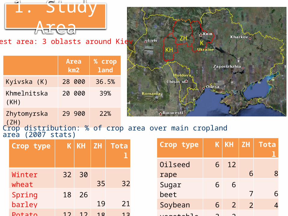
1. Study Area

Area km2 % crop land

Kyivska (K) 28 000 36.5%

Khmelnitska (KH) 20 000 39%

Zhytomyrska (ZH) 29 900 22%

Test area: 3 oblasts around Kiev

Crop type K KH ZH Total

Oilseed rape 6 12 6 8Sugar beet 6 6 7 6Soybean 6 2 2 4vegetables 3 2 3 2Sunflower 3 1 1 2

Crop type K KH ZH Total

Winter wheat 32 30 35 32Spring barley 18 26 19 21Potato 12 12 18 13maize 14 10 10 12

Crop distribution: % of crop area over main cropland area (2007 stats)

2. Hard classifications

• Ground survey + high resolution imagery land cover maps• Ground survey

– Segments & along the road• HR imagery

– AWIFS– Landsat 5 – TM– IRS LISS 3– RapidEye (RE)– Problem:

• Heavy cloud conditions in spring

• 10 Classes: Artificial-urban, winter (winter & spring wheat, rapeseed), spring (winter

& spring barley), summer (maize, potatoes, sugar beet, sunflower, soybean, vegetables), family gardens, other crops, woodland, permanent grassland, bare land, water & wetland

• For the sub-pixel approach merged winter & spring

3. Choice of high resolution LC map

1 Artificial2 'winter'3 'spring'4 'summer'5 Family garden6 Other crops7 woodland8 Perm grassland9 Bare land10 Water-wetland

• 75 scenes from 04 to 09• Overall accuracy MLP: 63%• Stripes at the overlapping areas of TM-frames

Masked

Landsat 5-TM (Kiev Oblast)

Hard classifcation map

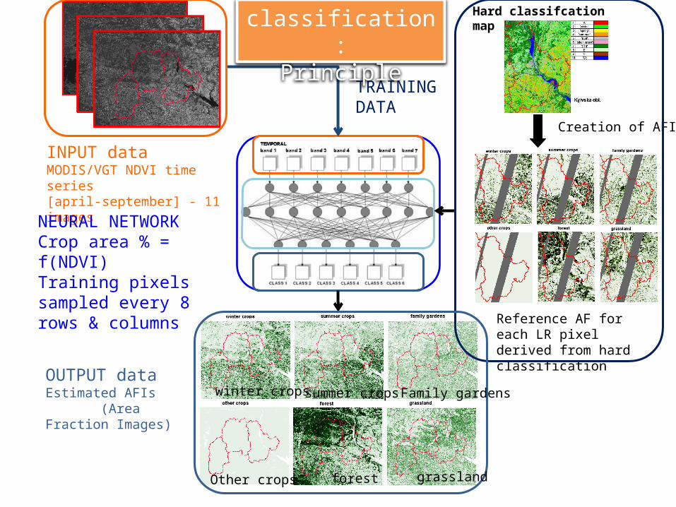
Creation of AFIs

Reference AF for each LR pixel derived from hard classification

INPUT dataMODIS/VGT NDVI time series[april-september] - 11 images

OUTPUT dataEstimated AFIs (Area Fraction Images)

NEURAL NETWORKCrop area % = f(NDVI)Training pixels sampled every 8 rows & columns

TRAININGDATA

LR soft classification:Principle

grasslandOther crops

winter crops summer crops

forest

Family gardens

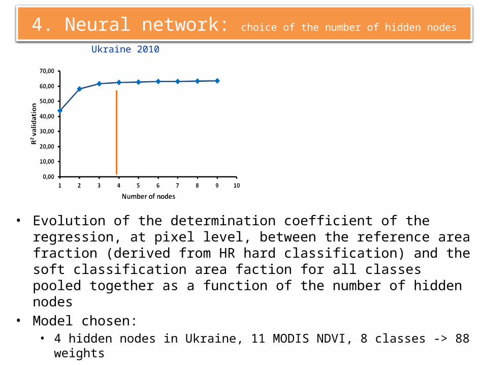
4. Neural network: choice of the number of hidden nodes

• Evolution of the determination coefficient of the regression, at pixel level, between the reference area fraction (derived from HR hard classification) and the soft classification area faction for all classes pooled together as a function of the number of hidden nodes

• Model chosen: • 4 hidden nodes in Ukraine, 11 MODIS NDVI, 8 classes -> 88 weights

Ukraine 2010

5. Assessment of crop area fractions at pixel level

• For Kiev oblast• Winter & spring crops

merged• All pixels considered for

the correlation

woodla

nd

sum

mer

cro

ps

win

ter-s

pring c

rops

fam

ily g

arden

s

grass

land

00.10.20.30.40.50.60.70.80.730000000000001

0.670000000000002

0.55

0.330000000000001

0.22

R2 between Estimated Area Fraction (output sub-pixel class) and Refer-

ence Area Fraction (TM)

6. Assessment at district levelCorrelation of class area fractions aggregated at district level for the Kiev oblast

woodland summer crops

winter-spring crops

family gardens

grassland0

0.10.20.30.40.50.60.70.80.9

1

R2 between Estimated Area Fraction (output sub-pixel class) and Reference

Area Fraction (TM)R2 pixel

R2 district

district

7. Use of soft classification with AFS•Predicting crop % from ground survey from class (winter crops, summer crops) % from soft classification•Area fractions aggregated per segment

0 5 10 15 20 25 30 35 40 45 500

10

20

30

40

50

60

f(x) = 0.746464809139354 x + 12.1540124236206R² = 0.437486646485907

Estimated AF - winter crops (%)

Ref

eren

ce A

FW

inte

r w

hea

t(%

) Winter wheat

0 10 20 30 40 50 600

10

20

30

40

50

60f(x) = 0.957304147413808 x + 11.8513341642218R² = 0.553644090696692

Estimated AF - summer crops (%)

Ref

eren

ce A

F M

aize

(%

)

Maize

crop R2

maize 0.55

Winter wheat 0.44

soybean 0.31

sunflower 0.10

Sugar beet 0.05

rapeseed 0.03

potato 0.01

II. North China Plain

1. Objective

• Problem: – difficulty of acquiring HR imagery at optimal timing– ground survey = cost and time consuming– Estimation crop areas for ongoing season

• Solution ?– Use the sub-pixel classification approach.– Spatial and temporal extrapolation of a Neural

Network

2. Temporal extrapolation

2005 2006 2007 2008 2009 2010 2011 2012 …

• 1. Perform a hard classification (ground survey, collection of high resolution data, classify) for a certain year.

• 2 .Use the hard classification and moderate resolution data of the reference year to train a neural network.

• 3. Apply the neural network on moderate resolution data for the consecutive years.

Condition : Interannual variation in temporal NDVI response is minor and has little effect on Neural Network performance (recognizing crop specific NDVI profiles).

Reference year

3. Spatial extrapolation

Training area

• 1. Perform a hard classification (ground survey, collection of high resolution data, classify) on a reference area.

• 2 .Use the hard classification to train a neural network.

• 3. Apply the neural network on moderate resolution data for a wider area.

Condition : Phenological differences over the region of interest is minor and has little effect on Neural Network performance (recognizing crop specific NDVI profiles).

2005

2006

2007

2009

2005: 2 TM classif2006: 1 LISS classif2007: 3 TM-classif

2 AWiFS classif2009: 1 TM classif 1 AWiFS classif

name = YYYYwt_sen• YYYY = year• wt = winter wheat• sen = sensor

4. Collection of hard classifications

Work on winter wheat estimations

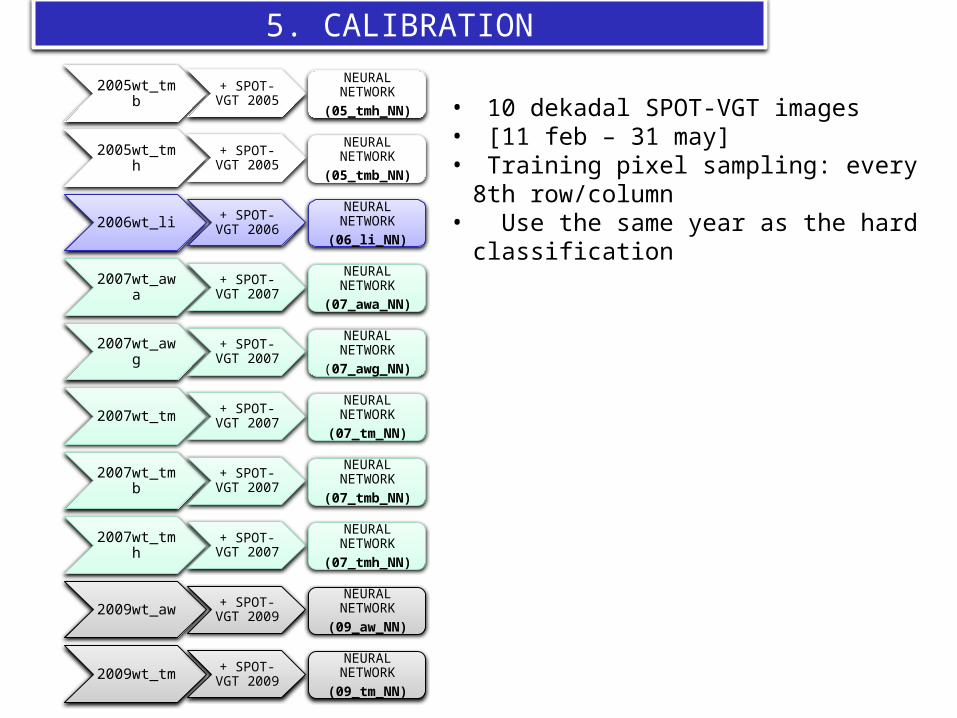
2005wt_tmb + SPOT-VGT 2005

NEURAL NETWORK(05_tmh_NN)

2005wt_tmh + SPOT-VGT 2005

NEURAL NETWORK(05_tmb_NN)

2006wt_li + SPOT-VGT 2006

NEURAL NETWORK(06_li_NN)

2007wt_awa + SPOT-VGT 2007

NEURAL NETWORK(07_awa_NN)

2007wt_awg + SPOT-VGT 2007

NEURAL NETWORK(07_awg_NN)

2007wt_tm + SPOT-VGT 2007

NEURAL NETWORK(07_tm_NN)

2007wt_tmb + SPOT-VGT 2007

NEURAL NETWORK(07_tmb_NN)

2007wt_tmh + SPOT-VGT 2007

NEURAL NETWORK(07_tmh_NN)

2009wt_aw + SPOT-VGT 2009

NEURAL NETWORK(09_aw_NN)

2009wt_tm + SPOT-VGT 2009

NEURAL NETWORK(09_tm_NN)

5. CALIBRATION

• 10 dekadal SPOT-VGT images• [11 feb – 31 may]• Training pixel sampling: every 8th

row/column• Use the same year as the hard

classification

6. APPLICATION

NEURAL NETWORK

INPUT = SPOT VGT data [11 feb – 31 may]

2005

2006

2007

2008

2009

2010

OUTPUT = 6 Estimated Area Fraction images for winter wheat, one for each

season

2005 2006

2007 2008

20092010

4 hidden nodes

1. Visual inspection crop patterns– Temporal and spatial consitency check

2. Compare with official statistics– Collection of official statistics for the 60 districts– [1994-2009]

7. VALIDATION

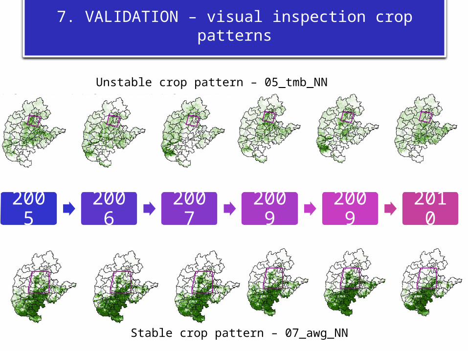
7. VALIDATION – visual inspection crop patterns

Unstable crop pattern – 05_tmb_NN

Stable crop pattern – 07_awg_NN

2005 2006 2007 2009 2009 2010

• For the 60 districts:– Collection of official statistics [1994-2009]– Caclulate the estimated crop areas for every sub-

pixel classification per district

7. VALIDATION – Compare with official statistics

7. VALIDATION – Compare with official statistics

Example: Comparisson Estimated Area Fraction for 2005with official statistics for 2005For the Neural Network 05_tmb_NN

1. Spatial 2. Scatterplot

7. VALIDATION – Compare with official statistics

07_awa_NN, 07awg_NN, 09tm_NN stable

05_tmb_NN

05_tmh_NN

06_li_NN

07_awa_NN

07_awg_NN

07_tm_NN

07_tmb_NN

07_awg_NN

09_aw_NN

09_tm_NN0

0.1

0.2

0.3

0.4

0.5

0.6

0.7

0.8

0.9Area estimates vs official statistics

20052006200720082009

Neural Network ID

R2 [d

istr

ict l

evel

]

7. VALIDATION – Compare with official statistics

Neural Network: 05_tmb_NN

R2 = 0.13 R2 = 0.07 R2 = 0.0 R2 = 0.21 R2 = 0.10

Neural Network: 09_tm_NN

R2 = 0.64 R2 = 0.77 R2 = 0.68 R2 = 0.74 R2 = 0.75

LOW PERFORMANCE

HIGH PERFORMANCE

• Heterogeneous reference dataset• single TM-frame HR classifications are not

capable to act as an input for the sub-pixel approach over the North China Plain

• mountain areas are known by strong underestimations– Winter wheat area is less important– Impact on results– Remove from further analysis

8. DISCUSSION

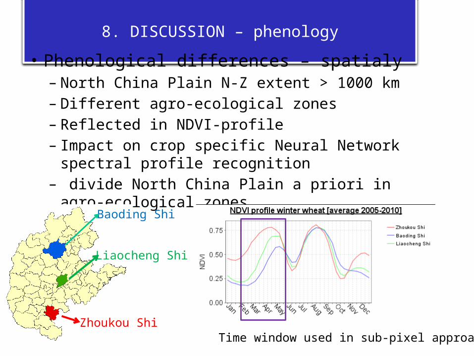
8. DISCUSSION – phenology

• Phenological differences – spatialy – North China Plain N-Z extent > 1000 km – Different agro-ecological zones– Reflected in NDVI-profile – Impact on crop specific Neural Network spectral profile

recognition– divide North China Plain a priori in agro-ecological zones

Zhoukou Shi

Liaocheng Shi

Baoding Shi

Time window used in sub-pixel approach

• Phenological differences – temporaly– Climatological conditions differ from year to year

8. DISCUSSION – phenology

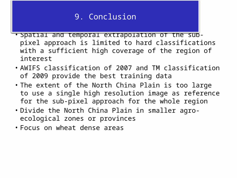
• Spatial and temporal extrapolation of the sub-pixel approach is limited to hard classifications with a sufficient high coverage of the region of interest

• AWIFS classification of 2007 and TM classification of 2009 provide the best training data

• The extent of the North China Plain is too large to use a single high resolution image as reference for the sub-pixel approach for the whole region

• Divide the North China Plain in smaller agro-ecological zones or provinces

• Focus on wheat dense areas

9. Conclusion

THANK YOU