Crime, Punishment, and Politics:An Analysis of Political Cycles in Criminal Sentencing.

Carlos Berdejo Noam Yuchtman∗

April 2012

Abstract

We present evidence that Washington State judges respond to political pressure by

sentencing serious crimes more severely. Sentences are around 10% longer at the end of

a judge’s political cycle than at the beginning; judges’ discretionary departures above

the sentencing guidelines range increase by 50% across the electoral cycle, accounting

for much of the greater severity. Robustness specifications, non-linear models, and fal-

sification exercises allow us to distinguish among explanations for increased sentencing

severity at the end of judges’ political cycles. Our findings inform debates over judicial

elections, and highlight the interaction between judicial discretion and the influence of

judicial elections.

JEL Codes: K40, K42, D72

∗Berdejo: Loyola Law School, carlos.berdejo@lls.edu; Yuchtman: Haas School of Business, UC-Berkeley,yuchtman@haas.berkeley.edu. We thank the editor, Dani Rodrik, and two anonymous referees for theirextremely helpful comments. We also thank Ernesto Dal Bo, Larry Katz, and Andrei Shleifer for theirfeedback and encouragement, as well as participants at the Harvard Labor Lunch, the MIT Political EconomyBreakfast, the Harvard Law, Economics and Organizations Seminar and the 2009 Annual Meeting of theAmerican Law and Economics Association. The authors gratefully acknowledge financial support from theHarvard Center for American Political Studies.

1

1 Introduction

Whether judges should be subject to electoral review has long been debated in designing

constitutions and judicial systems1 and has received recent attention in both the legal and

economic literature, as well as in the popular press.2 Editorialists, jurists – notably, retired

Supreme Court Justice Sandra Day O’Connor – and private organizations have expressed

concern that judicial decision making could be influenced by political pressure, to the detri-

ment of the public.3 Researchers have endeavored to determine whether judicial behavior

responds to differences in political environments, part of a large literature examining judges’

responses to the incentives and constraints they face.4 Such work not only informs our

understanding of the judicial branch, but is also relevant to the broader political economy

question of the effect of political pressure and electoral accountability on public servants’

behavior.5

Much of the existing literature on the impact of judicial elections on judges’ behavior has

used cross-state variation in retention methods to identify elections’ effects (for example,

Besley and Payne (2005)). A weakness of this methodology is that differences in retention

methods across states could be correlated with unobservable factors that affect the outcome

of interest.6 Prior work has also generally ignored criminal case outcomes in courts of general

jurisdiction. Work on criminal case outcomes has focused on higher courts (for example,

Hall (1992) and (1995)). Most studies analyzing lower courts have examined civil cases (for

example, Hanssen (1999), Tabarrok and Helland (1999), and Besley and Payne (2005)).

One might prefer to focus on criminal case outcomes in lower courts for several reasons.

First, the stakes are high: depending on the outcome of a criminal case, the state may

deprive a citizen of his rights, property and even his life. Because courts of appeals give

considerable deference to the findings of facts by trial courts and, in states with determinate

2

sentencing, convicted felons serve their full sentences, trial court outcomes are paramount.

Second, crime is an issue about which the citizenry has well defined preferences. In addition,

since convicted felons lose their right to vote in most states (including Washington, see RCW

9.94A.637), they could be an attractive target for politically opportunistic judges.

Several recent papers have focused on the impact of politics on criminal case sentencing. Lim

(2008) estimates a structural model of felony sentencing by Kansas judges and finds that

judges in counties using partisan judicial elections exhibit different sentencing patterns from

judges in counties using referendum judicial elections. These different patterns are attributed

both to different preferences and to the effects of elections on judges’ behavior. Gordon and

Huber (2004) and (2007) estimate the effect of the proximity of a judge’s retention election on

that judge’s sentencing decisions using data from Pennsylvania and Kansas. In Pennsylvania,

where judges are retained in referendum elections, they find that sentencing becomes more

severe as elections approach (that is, sentencing severity exhibits “cycles” corresponding to

the political calendar); however, they do not find sentencing cycles in Kansas counties where

judges are so retained. Gordon and Huber do find sentencing cycles in Kansas counties where

judges are retained in partisan elections.

We also examine the impact of elections on judicial behavior by testing for the presence of

political sentencing cycles. Under a broad range of specifications, we find that sentencing

of serious offenses becomes more severe as elections approach – sentence lengths increase by

around 10% between the beginning and the end of a judge’s political cycle. In contrast to

much of the existing literature, we are able to test – and rule out – alternatives to the hy-

pothesis that longer sentences are the effect of political pressure on judges. First, we directly

examine case characteristics (including variables that reflect the result of any bargaining

between the defense and district attorneys) across judges’ political cycles, and do not find

evidence that these systematically vary across the judge’s political cycle. A range of specifi-

3

cations suggests that changes in the behavior of defense and district attorneys across judges’

political cycles do not explain the sentencing cycles we observe. We distinguish between

judicial political cycles and the political cycles of other officials by exploiting differences in

the timing of electoral pressure across offices, and exploring non-linear models of the effect

of electoral proximity. We find that sentence lengths exhibit a break precisely at the end of

judges’ political cycles, but not at the end of the political cycles of other officials. We can

rule out cyclical patterns in sentencing due to factors other than politics (e.g., variation in

unobservable case characteristics) by examining sentencing by retiring judges, who do not

face electoral pressure; the sentencing of less serious crimes, about which the public (and

potential competitors for a judge’s seat) are likely less concerned; and, sentencing in nearby

Oregon, where judges are elected on a different cycle. We do not find sentencing cycles

for retiring judges in their final term, or cycles for less serious crimes; sentencing in nearby

Oregon does not follow the Washington pattern. All of this analysis provides evidence of

large and statistically significant sentencing differences in judges’ sentencing behavior in re-

sponse to political pressure. To better understand the nature of these sentencing cycles, we

consider multiple outcome variables, shedding light on the role played by deviations outside

the sentencing guidelines range. We find that deviations above the range increase by 50%

across a judge’s political cycle and account for a large part of the cycles in sentence length,

suggesting that the effect of political pressure on sentencing is mediated by the availability

of judicial discretion.

In what follows, we discuss judicial elections and criminal sentencing in the state of Wash-

ington in Section 2. In Section 3, we describe and provide empirical support for a theoretical

framework that predicts sentencing cycles as a result of political pressure on judges. In Sec-

tion 4, we discuss our data and the construction of the variables used in our analysis. We

present our empirical model and results in Section 5, and finally discuss the implications of

our findings and conclude in Section 6.

4

2 Judicial Elections and Criminal Sentencing in Wash-

ington

The structure of judicial elections and the laws governing sentencing provide the context for,

and inform, our empirical analysis of judges’ behavior.

2.1 Judicial Elections

Washington Superior Courts are currently organized into 32 judicial districts, either a county,

or a group of adjacent counties,7 and Superior Court judges are elected and retained via

nonpartisan elections every four years (coinciding with presidential election years).8 Judicial

candidates are required to file for public office by the filing deadline – in our sample period

the last Friday of July – and if more than one candidate files for a given seat, the candidates

face each other in the primary elections (held in September). If no candidate receives more

than 50% of the vote in the primary election, the two candidates with the most votes face

each other in the general election (held in November).

For our purposes, judges’ political cycles end either at the filing deadline, after which the

threat of a challenger in the upcoming election no longer exists, or at the primary or general

election, depending on the entry and success of challengers.

2.2 Criminal Sentencing

Criminal sentencing in Washington for felony crimes is governed by the 1981 Washington

Sentencing Reform Act (WSRA), which established presumptive sentencing ranges based on

the conviction offense and the defendant’s criminal history.9 The Washington guidelines are

5

relatively simple and transparent, especially in cases that are adjudicated via plea agreements

(the vast majority of Washington cases), as the plea agreement itself includes the guidelines

cell, including any enhancements (the relevant page from the Washington plea agreement

form is in the Online Appendix, Figure A2).

For each case, then, the applicable range of the sentencing guidelines cell can be thought

of as the basic constraints on judicial discretion, which the judge takes as given.10 In our

baseline empirical analysis, we will consider the use of judicial discretion controlling for the

guidelines range that applies to a given case, as well as a dummy variable indicating the type

of adjudication (plea or trial). This specification allows us to isolate the variation in sentence

severity due to changes in judges’ behavior across their political cycles: by conditioning on

the outcomes of attorneys’ bargains, we hope to remove any effect of changed outcomes of

attorneys’ bargains from the relationship we estimate between political pressure on the judge

and sentence severity.

Of course, plea agreements and guidelines cells are negotiated by attorneys in the shadow of

the trial judge (see, for example, Reinganum (1988), Lacasse and Payne (1999), and Bibas

(2004)), and thus might endogenously respond to changes in political pressure on the judge.

To address this concern with our baseline empirical model, in our empirical analysis below we

also examine the shifting of cases across adjudication categories, across sentencing guidelines

cells, and across time.

Prior to the Blakely decision of 2004,11 Washington Superior Court judges had full discretion

to select a sentence within the applicable range, and could sentence outside the standard

range upon making certain findings (see RCW 9.94A.390). In practice, deviations outside

the range were quite unusual: in our sample of felony convictions, judges imposed sentences

above the range in fewer than 3% of cases (and in 6% of the serious crimes on which we focus).

If the judge found that an exceptional sentence was warranted, the sentence length was left to

6

his discretion, but was subject to appellate review. After Blakely, a judge may still sentence

anywhere within the applicable range in the sentencing grid, but cannot impose a sentence

above this range unless the jury finds, or the defendant pleads to, special circumstances

prescribed by statute.

Under the WSRA, an individual convicted of a felony offense occurring on or after July

1, 1984, receives a determinate sentence and, as a result, is expected to serve the sentence

in full. This is important since the existence of a parole board that conditions the release

dates of convicted felons on recidivism risk could mitigate any social welfare consequences

of excessive sentences.12

3 Theoretical Framework

There exists a large literature, both theoretical and empirical, on political cycles among

executive and legislative government officials (for example, Nordhaus (1975), Rogoff and

Sibert (1988), Alesina and Roubini (1992), and Akhmedov and Zhuravskaya (2004)); for

a recent overview of empirical evidence, see Franzese (2002). In these models, there is a

principal-agent problem with moral hazard: officials are voters’ agents, and voters reward

performance in office with their votes because they attribute good performance either to the

incumbent’s ability or to his willingness to further the electorate’s interest rather than his

own. If voters or potential challengers (who can inform voters) monitor and evaluate officials

around the time of an election, there will exist incentives for the incumbent to perform well

(i.e., perform as voters prefer) precisely at this time. Cyclical behavior across an official’s

term can also arise from time discounting: early in their terms, officials will behave according

to their own preferences, while late in their terms they will place more weight on maintaining

their official positions, and thus behave according to voters’ preferences.13

7

Elected judges in Washington State face political pressure similar to that faced by other

elected officials. They are voters’ agents, and there exists a divergence between voters’

preferences and judges’: voters prefer more severe penalties than judges hand down. We

review the General Social Surveys (GSS) from 1972–200614 and find that when asked whether

“the courts in [the respondent’s] area deal too harshly or not harshly enough with criminals?,”

82.8% of the respondents answered that courts are “not harsh enough”, while only 12.2%

and 5.1% believed that courts were “about right” or “too harsh”, respectively.15 These

differences in sentencing preferences may arise from various factors. First, judges do not like

being reversed, and they can be reversed in a criminal case if their judgment results in a

conviction, or (in Washington State) if the sentence they impose is higher than the high-end

of the applicable guidelines range. Second, the public may have a biased perception of the

average criminal (or crime), for example, as a result of the portrayal of crime in the media.

Third, the judge has to personally confront the person who is being sentenced, which may

make extremely punitive sentencing more costly. Finally, judges are, on average, better

educated than voters, and may be systematically different in other ways (culturally, socially,

politically), which could lead them to prefer more lenient sentences. Regardless of the reason

for the divergence in preferences, there is good reason to believe that judges might sentence

more severely in order to please voters.

Of course, judges will only change their behavior in response to political pressure if there

is some possibility that voters will punish them for sentencing too leniently. For voters to

do so, they must vote in judicial elections, and they must have access to information on

judges’ sentencing. To explore the issue of turnout, we collected voting data for two counties

(King and Yakima) in the 2004 judicial election cycle. In Yakima County, voter turnout for

the Superior Court race during the 2004 General Elections was 9% higher than the turnout

for the three Supreme Court races and 90% of the turnout for the gubernatorial election.

During the 2004 primaries, voter turnout for the Superior Court race was 11% higher than

8

the turnout for the three Supreme Court races and 93% of the turnout for the gubernatorial

primaries.16 In King County, voter turnout for the two Superior Court races during the 2004

General Elections was 95% of the turnout for the three Supreme Court races and 73% of the

turnout for the gubernatorial election. During the 2004 primaries there were three contested

seats and voter turnout for these races was 98% of the turnout for four Supreme Court

races and 70% of the turnout for the gubernatorial primaries.17 Although these numbers are

anecdotal, they suggest that the public does vote in Superior Court elections.

The next question is whether voters have information on judges’ sentencing behavior. A

natural monitor of judicial behavior, and potential source of such information to the elec-

torate, is the media. Using Lexis-Nexis, we search major Washington newspapers18 to assess

the frequency of stories involving Superior Court judges; and, to provide some perspective,

we compare it to the frequency of news stories involving other elected city officials.19 For

the period July 1995–December 2006, there were 13,404 stories involving Superior Court

judges compared to 14,434 involving city council members.20 Of the 13,404 stories involving

Superior Court judges, 4,603 also involve sentencing.21

Importantly, newspapers focus on the serious crimes about which the public is likely most

concerned: those classified by the FBI Uniform Crime Reporting Program (UCR) as violent

crimes, namely murder and non-negligent manslaughter, forcible rape, robbery, and aggra-

vated assault. Out of the 4,603 stories involving sentencing by Superior Court judges, 3,671

(79.75%) involve at least one of the four crimes labeled as violent by the UCR.22 These

results support our use of the UCR-inspired set of visible crimes as the subset of crimes on

which we focus our empirical work.

Potential challengers have an incentive both to monitor incumbents’ current behavior and to

research their past behavior; and, when they officially challenge an incumbent, challengers

have the incentive to provide this information to the public. In their study of print media

9

and judicial elections in Wisconsin, Kearney and Eisenberg (2002) find that in state Circuit

Court (analogous to Washington’s Superior Court) races, advertising by judicial candidates

dominates newspaper articles as a means of disseminating information about judicial candi-

dates. In addition, the authors find that advertisements often touch upon criminal matters.

We have reviewed Washington judicial candidates’ websites and voter pamphlets (from the

2008 election cycle) and find that crime and sentencing are among the issues discussed by

challengers.23

One might wonder whether the threat of competition can keep judges’ behavior consistently

in line with voters’ preferences (resulting in no cyclicality in sentence severity). There are

several reasons why incumbent judges may tend to sentence leniently early in their terms and

more severely toward the end, despite the threat of competition. First, if monitoring a judge’s

sentencing is costly, potential challengers might only do so when they are considering entering

a race – which occurs late in a judge’s term. Because researching past sentencing is costly

for a challenger, they will likely invest more effort in observing current judge sentencing,

making it less costly for a judge to behave as he likes early in his term. Second, even if a

potential challenger informs voters of a lenient sentence from a judge’s past, this information

may influence voters less than information on more recent sentences – again, this would lead

a judge to sentence relatively leniently early in his term. Finally, to the extent that the judge

discounts the future, this would only make more pronounced his tendency to sentence severely

only at the end of his term. Thus, we expect incumbent judges will sentence most severely

close to the deadline for competitors to file to enter a race: this is when incumbents are most

likely to be monitored, and when they place the greatest weight on voters’ preferences.

Thus, just as executive or legislative officials are incentivized to lower taxes or increase public

spending before their elections to avoid being punished in the polls, judges face analogous

pressure to impose longer sentences as they near the end of their political cycles. We next

10

test whether they respond to this pressure by sentencing more severely.

4 Data and Construction of Variables

4.1 Description of the Dataset

We obtained case-level data from the Washington State Sentencing Guidelines Commission

(“SGC”) on criminal sentencing in felony cases. The dataset includes 294,349 observations

from the period July 1995 through December 2006. The data include information on case-

specific variables such as defendant characteristics (for example, race, criminal history, etc.),

date of sentence, name of judge, conviction offense, low- and high-end of the applicable

sentencing guidelines range (including enhancements), type of adjudication (plea or trial),

and sentence length, for the most serious conviction offense (among other variables). We

augment the data received from the SGC with information on judges, judicial districts, and

judicial elections, as described below.

We restrict the sample of cases used in our analysis in several ways. We only include cases

heard by judges serving in the Superior Court, the court of general jurisdiction for criminal

cases. Cases heard by judges who were serving on the Superior Court as commissioners, in

a pro tem capacity, or who were serving as District Court judges at the date of sentence, are

excluded from our sample. Each Superior Court judge is matched to one of Washington’s

judicial districts, and we exclude cases heard by a judge outside his home district (judges

may appear in multiple districts either because of measurement error or because they are

acting as “visiting” judges in a neighboring district). We also exclude cases heard by judges

with fewer than 25 cases in the sample, cases heard by judges appointed to fill a mid-term

vacancy prior to their first election, and cases in which the judge has no sentencing discretion.

11

We also classify crimes according to classes based on two-digit offense codes (provided by

the SGC), and restrict our analysis to those felony classes for which there were at least 100

cases.

After applying these restrictions, there remain 276,119 cases heard by 265 full-time Superior

Court judges for the period between July 1995 and December 2006 (the Online Appendix,

Table A1, contains case-level summary statistics for this sample). Our empirical analysis

will focus on the most serious, visible crimes (as defined by the FBI, described in Section 3):

assault, murder, rape and robbery, which make up 6.7% of the entire sample (18,447 cases).

Among these visible crimes, 8% of defendants are women and 24% are black; around 53%

have at least one prior conviction; the vast majority of cases are resolved via plea agreement

(over 88%). The average case is associated with a 51 month low-range sentence from the

sentencing guidelines grid, and a 67.6 month high-range; the average sentence is 67.2 months.

Around 6.3% of cases result in sentences greater than the high-end of the guidelines range.

On average, cases are heard almost exactly halfway into a judge’s election cycle (see Table

1 for case-level summary statistics).

Of the 265 judges in our dataset, 29% are women and 5% are Black; judges on average were

admitted to the Washington Bar in 1974 and took their seats on the Superior Court in 1992.

36% of judges had some prior experience as prosecuting attorneys; 46% had previous judicial

experience. In the time period on which we focus (1995–2006), we observe 456 seated judges

filing for re-election. Of these judges, 39 (8.4%) faced competition in a primary election,

and 4 (.87%) faced competition through a general election (the Online Appendix, Table A2,

contains summary statistics for the 265 judges).

12

4.2 Construction of Variables

We examine several different sentencing outcomes in our analysis. Our primary measure

of sentence severity is the length of a prison or jail sentence in months, top-coded at 720

months (following Abrams et al. (2008)). We also consider sentence lengths with a top-code

of 1,200 months; in some specifications we censor sentence length at the high- and low-end

of the applicable sentencing range. Finally, we consider a binary outcome variable equal to

one if a judge imposed a sentence above the high-end of the guidelines’ range for a case.

The explanatory variable of interest is the electoral pressure on a case’s judge, in particular,

the proximity of the judge’s next election or filing deadline (information on which was com-

piled from the Washington Secretary of State’s website, various county auditor websites, and

county election websites). We construct both linear and nonlinear measures of electoral prox-

imity. The linear measure of electoral proximity is, in general, for case i, heard by judge j,

sentenced at time t, the number of days between time t and the next election’s filing deadline

for judge j, divided by 1,461 (the number of days in four years, a full election cycle).24 This

measure, which we call linear distance, ranges from 0 to 1, with 0 implying maximal elec-

toral pressure. When a judge faces a competitor for his seat, we set our proximity measure

equal to 0 for any cases sentenced between the filing deadline and the date that an election

determines the winner of the seat. Based on this linear measure of electoral proximity, we

construct a set of dummy variables that indicate the number of quarters remaining until a

judge’s upcoming filing deadline, ranging from one to sixteen (with any cases between the

filing deadline and the end of that judge’s election cycle included in the 1-quarter-to-election

period).

Case-specific controls include defendant’s age, gender, race, and prior criminal history; an

indicator of whether the sentence resulted from a plea agreement; a set of offense-specific

13

indicator variables; and, the applicable sentencing guidelines range for each case. Addition-

ally, we construct a set of fixed effects for the cell in the Washington Sentencing Guidelines

Grid in which a case is located. The cells are constructed based on the high- and low-end

of the sentencing guidelines range, including all enhancements. In order to avoid estimates

based on cells with very few cases, we consider a variety of methods of grouping cases that

are in the most unusual cells, grouping them 100, 150, or 200 at a time.

To control for changes in sentencing behavior resulting from the Blakely decision, we generate

an indicator variable equal to 1 if the case’s sentence date was after June 24, 2004. We also

generate a set of year-specific fixed effects to capture shocks affecting criminal sentencing

that are common to all judges in a given year, and a set of fixed effects for each quarter of the

year (January through March, April through June, etc.), which control for any seasonality

in judges’ sentencing behavior.

A set of judge fixed effects controls for differences in sentencing across judges and a set of

judicial district fixed effects controls for time-invariant features of a district (for example,

stable differences in the various district attorneys’ offices). We also collected information on

time-variant judicial district characteristics: unemployment rates and crime rates (see the

Online Appendix, Table A3, for a detailed description of the names, definitions, and sources

of all variables used in our empirical analysis).

14

5 Empirical Model and Results

5.1 Empirical Model and Identifying Assumptions

As described above, we constructed a dataset by merging case-level information provided by

the SGC to information on districts and judges compiled from a variety of sources. The unit

of observation in our dataset is the case, i, heard by judge j, sentenced at time t. Each case

is associated with a specific offense, defendant, judge, sentence date, and sentence.

Our empirical model is the following:

severityijt = F (t) + β1Proxijt + β2Zijt + εijt (1)

where, severityijt is a sentencing outcome associated with case i ; F(t) includes a set of

year and quarter fixed effects, as well as a dummy variable indicating whether case i was

decided after the Blakely decision; Proxijt, our explanatory variable of interest, is a measure

of electoral proximity (linear or nonlinear); Zijt contains a set of defendant, crime, and

sentencing guidelines controls, as well as a full set of judge and judicial district fixed effects;

finally, εijt is a mean-zero stochastic error term.

This baseline empirical specification goes beyond just examining the reduced form relation-

ship between judicial elections’ proximity and sentencing (though this reduced form rela-

tionship is in itself interesting). It incorporates various aspects of the structure and timing

of judicial procedure in Washington State in order to try to identify changes in judges’ be-

havior per se. In particular, two crucial outcomes of attorneys’ actions – whether a case is

adjudicated via plea or trial, and the sentencing guidelines cell in which a case falls – are

determined prior to a judge’s sentencing decision, and are observed in our dataset. In the

15

baseline analysis, we control for variation in the type of adjudication and the sentencing

guidelines cell in which each case fell, thus “purging” from the estimated effect of electoral

proximity that part which works through attorneys’ bargaining. Under the identifying as-

sumptions that cases are randomly assigned across the judge’s political cycle (conditional

on controls) and that the attorneys’ negotiation process does not change across the judge’s

political cycle – both assumptions that we examine in detail – this specification allows us

to estimate the effect of judicial elections’ proximity working through changes in a judge’s

sentencing, conditional on the outcomes of attorneys’ negotiations.

Before presenting our baseline empirical results, it is important first to consider the fun-

damental identifying assumptions that need to be satisfied for our estimate of β1 to be an

unbiased estimate of the impact of judicial elections’ proximity on the sentences that judges

impose. We begin by examining whether cases are randomly assigned across the political

cycle, conditional on the control variables included in the model. Next, we will take up the

issue of endogenous outcomes of attorney negotiations (and we return to both of these issues

again in Section 5.3).

In practice, an important concern is that aspects of a case that we cannot observe (some

characteristics of the crime, of the criminal, etc.), and that affect sentencing, are changing

over time in a way that is correlated with our measure of electoral proximity. This might

arise from the strategic behavior of attorneys or the judge, or might be due to other sources

of variation from outside the judicial system (e.g., changes in policing). While we cannot

directly test for systematic variation in unobservable characteristics across the political cycle,

we attempt to address this issue as rigorously as possible.

We begin by simply examining observable case characteristics just before (and during) the

judicial election period, and compare them to cases just after the judicial elections. If

observables are balanced across the political cycle, one might believe that unobservables are

16

balanced, too. In Table 2, columns 1–2, we present summary statistics for serious, visible

crime cases sentenced in the two quarters before a judge’s filing deadline (and up to his

election, when applicable), as well as the analogous statistics in the two quarters after a

judge’s filing deadline or election (see the Online Appendix, Table A4, for a comparison of

case characteristics around the filing deadline for all crimes). Importantly, visible crimes

make up a similar proportion of all cases before and after elections, around 6.9%. For the

serious, visible crimes, both defendant and case characteristics look very similar just before

and just after judicial elections (p-values testing for equality of means are reported in column

3). Women make up around 8.5% of the sample in both periods; black defendants around

25%; around 51% of defendants have at least one prior conviction. Most of the data in Table

2, columns 1–3, are consistent with random assignment of cases across judges’ political cycles.

Some case characteristics do differ across periods. The most important of these is the frac-

tion of cases adjudicated by plea agreement: 87.7% just before elections and 89.2 just after

elections, a marginally significant difference. This difference immediately raises the ques-

tion of endogenous attorney negotiation across judges’ political cycles. It is reassuring to

see that the high-and low-end of the sentencing guidelines range reveal no significant differ-

ences in Table 2 (this suggests that neither judges nor attorneys successfully manipulate the

sentencing guidelines range), but we must examine attorneys’ bargains in greater depth.

Pleas might differ across the political cycle simply because of natural variation in case char-

acteristics; in that case, we would simply want to control for whether a case resulted in a plea

or trial. On the other hand, the changing rate of plea agreements might systematically alter

the types of cases ending in plea agreement across judges’ political cycles. To see whether

the difference in plea agreements seems to shift the types of cases in a given category, we

check for balanced characteristics within adjudication categories across the election cycle.

In Table 2, columns 4–9, we present summary statistics just before and just after elections,

17

along with tests for equality of means, for pleas alone and for trials alone. In both cases, one

can see that observable case characteristics are quite balanced across the election cycle: for

example, it is not the case that pleas just before and after the cycle end up with significantly

different sentencing guidelines ranges.

To examine the potential endogeneity of pleas and sentencing guidelines range outcomes

more systematically, we regress these outcomes on linear distance (our explanatory variable

of interest in the baseline model), as well as year and quarter-of-the-year fixed effects (which

control for changes in case characteristics across time). In all three regressions, the outcomes

of attorney negotiations are not significantly associated with our measure of political pressure

on the judge: p-values testing for a significant relationship range from 0.28 to 0.76. We also

examined whether these outcomes were systematically different in the last six months of

the judge’s political cycle (relative to the rest of the cycle), regressing the three negotiation

outcomes on a dummy indicating that a case was sentenced in the last 6 months of a judge’s

political cycle, year fixed effects, and quarter-of-the-year fixed effects. Again, p-values testing

for a significant relationship between the political cycle and attorneys’ negotiations are quite

high: between 0.24 and 0.65. Finally, we ran 115 regressions with an indicator for each

sentencing guidelines cell as the outcome, and an indicator that a case was sentenced in

the last six months of the political cycle as the explanatory variable of interest (using our

baseline specification). In only five of these is the coefficient on the “last six months”

indicator significant – cells are distributed essentially randomly across the political cycle.25

We will return to concerns about endogenous attorney bargains in Section 5.3.1, and take

up more general concerns about unobservables correlated with judges’ political cycles in

Sections 5.3.2 and 5.3.3. For now, given the reassuring evidence on the distribution of cases

and attorneys’ negotiations across judges’ political cycles, we will estimate our baseline

specification, controlling for the type of adjudication and the guidelines cells.

18

5.2 Baseline Results and Sensitivity Analysis

We begin our examination of sentence severity across judges’ political cycles by presenting

the sentencing patterns for serious, visible crimes in the raw data. We simply plot the average

difference between the sentence length and the high-end of the applicable guidelines range,

by the number of quarters remaining until the next election or filing deadline (see Figure 1).

In this graph, one observes an increase in sentence length from the beginning of the political

cycle to the end, and a sharp decline in the severity of sentences just after the cycle ends. In

addition, sentences in the final year of the political cycle are, on average, above the high-end

of the guidelines range; this is almost never the case during the first three years of the cycle.

To examine this relationship more rigorously, we estimate equation (1) for visible crimes using

a linear measure of electoral proximity (linear distance) and a full set of control variables,

and using the sentence length in months, capped at 720 months, as our outcome variable.

This specification covers three judicial elections: 1996, 2000, and 2004. If judges sentence

more harshly as their elections approach, one would expect distance to the election to be

negatively correlated with sentence length; and, as can be seen in Table 3, column 1, this

is exactly what we find. We estimate that moving from the beginning of a judge’s election

cycle to the end adds a statistically significant 6.8 months to a defendant’s sentence.26 This

represents over 10% of the average sentence for visible crimes in our sample.27

We next check the robustness of our results to the cases included in our empirical analysis.

One may be concerned that the Blakely decision, which significantly reduced judicial discre-

tion, may confound our estimates. To address this, we estimate equation (1) as above using

only cases decided pre-Blakely (see Table 3, column 2). One might worry that murder cases

are driving our results: because murder convictions will often produce very long sentences,

including murder cases might allow outlying sentences to have undue influence.28 We thus

19

estimate equation (1) only for visible crimes other than murder (see Table 3, column 3).

Finally, we estimate equation (1) only on cases adjudicated by plea agreement (see Table

3, column 4). In all three of these specifications, our estimated coefficient is negative, sta-

tistically significant, and large. Even for cases adjudicated by plea agreements, where one

might expect judicial discretion to be more limited, the estimated coefficient is over 6% of

the mean sentence for visible crimes.29

It is also important to evaluate the robustness of our results to the specification choices

that we made. One concern is that our measure of electoral proximity is endogenous: if

severe sentences make it less likely that an incumbent judge will face a challenger, then

our proximity measure will be endogenous. Thus, we estimate our baseline specification

using a purely exogenous measure of linear distance which only uses the time until the next

filing deadline to measure electoral proximity (see Table 3, column 5).30 Another issue is

our method of controlling for the guidelines range relevant to each case. In our baseline

estimates (Table 3, column 1), we used cells constructed based on the low- and high-end

of the range for each crime; and, for crimes in cells with fewer than 150 cases, we grouped

crimes, 150 at a time, based on similarity of the low-end of the range for each crime.31 One

might be concerned about grouping crimes with different low- and high-end ranges. To see

whether this grouping of crimes affects our results, we use only cases in cells that contain

50 or more observations, dropping cases in the most unusual cells instead of grouping them

(see Table 3, column 6). To determine whether our results depend on the use of any sort of

cells as controls, we consider estimates that simply control linearly for the low-end and the

high-end of the sentencing range applicable to the case (see Table 3, column 7). Under all

of these alternative specifications, we find significant and large sentencing cycles of around

10% of the average sentence length in the relevant sample.

Next, we estimate equation (1) on an extended dataset, covering the period 1985–2006,

20

which includes five judicial elections.32 This dataset, also provided to us by the Washington

SGC, does not have as much information as our 1995–2006 dataset; in particular, it lacks

information on each case’s judge. Thus, we simply assign each case a linear electoral prox-

imity measure based on the upcoming election’s filing deadline. The estimates using these

data will be imperfect, but they should reassure the reader that our estimates in Table 3,

columns 1–7 were not the product of too few election cycles. These results are also based on

an entirely exogenous measure of electoral pressure, as they do not incorporate information

on competition. We thus estimate equation (1) using the entire 1985–2006 time period, and

again find a statistically significant, negative, and large coefficient on linear distance (see

Table 3, column 8).33

Finally, we use the log of the sentence length (plus 1) as the outcome in our regression, as this

has been standard in the empirical literature on sentencing. We prefer the levels specification

since adding 1 to the sentence length to avoid dropping sentences of length 0 is arbitrary; in

addition, the log transformation of the outcome variable reduces the variation from which

we identify the effect of electoral proximity, especially for longer sentences. Nonetheless, we

observe statistically significant sentencing cycles in this specification as well (see Table 3,

column 9).34

We report several other robustness checks in the Online Appendix. First, because we include

many fixed effects in our baseline specification, we estimate equation (1), but use judge

characteristics instead of judge fixed effects. To test the sensitivity of our results to the

choice of 720 months as a top-code for our outcome variable, we estimate equation (1), but

use the sentence length in months capped at 1,200 months as our outcome variable. Our

baseline results are robust to all of these specification choices (see the Online Appendix,

Table A6, columns 3–5).

The results presented in Table 3 are striking: essentially the same defendant (based on

21

observable characteristics), having committed the same crime, facing the same judge, with

his case ending in the same sentencing guidelines cell, receives a significantly longer prison

sentence if he is sentenced at the end of the judge’s political cycle rather than the beginning.

This result is robust to a wide range of different specification choices, the exclusion of murder,

and the construction of guidelines cells. It is also robust to examining the five judicial

elections between 1985 and 2006.

5.3 Ruling out Alternative Hypotheses

The results presented thus far strongly suggest that greater electoral proximity for a case’s

judge is associated with a longer sentence for that case. However, one could conceive of

explanations for the relationship observed other than judges responding to political pressure.

Here we evaluate several alternative explanations for our results: first, we consider changes

in the behavior of the defense attorney and the prosecutor; next, we consider the effects of

the political cycles of officials other than judges; finally, we consider changes in unobservable

case characteristics across judges’ political cycles more generally.

5.3.1 Does Attorneys’ Behavior Change Across Judges’ Political Cycles?

In our baseline estimates, we attempted to identify judges’ (as opposed to attorneys’) re-

sponse to political pressure by controlling for the outcomes of attorneys’ negotiations. We

now explore changes in attorney behavior across judges’ political cycles in more depth. We

consider, in turn, the changing rate of plea agreements across judges’ political cycles (also

discussed in Section 5.1); the roles of changing plea agreement practices and sentencing

guidelines cells in generating sentencing cycles; and, finally, the shifting of cases across time

by attorneys (or judges).

22

Our results in Table 2 raised some concerns about differences in the types of plea agreements

reached across judges’ political cycles. Moreover, Piehl and Bushway (2007) find that charge

bargaining and prosecutorial discretion in negotiating pleas are important in Washington.

If the bargains struck varied across judges’ political cycles – perhaps because attorneys

understood that judges’ incentives differed – this could affect both the rate of pleas across

the cycle, and also the types of cases in each adjudication category. For example, if cases

with “worse” unobservable characteristics were adjudicated by plea toward the end of judges’

political cycles, simply controlling for the adjudication type would not be enough. One

might worry that the association between judicial elections’ proximity and sentence severity

observed in our baseline specification resulted from mis-specifying the effect of the type of

adjudication on sentence length. To address this concern, we estimate our baseline model,

but now include an interaction between the type of adjudication (a “trial” dummy variable)

and linear distance. The coefficient on linear distance here captures the impact of elections’

proximity on sentencing for pleas, which will allow for a comparison with the “pleas only”

specification presented in Table 3, column 4.35 As can be seen in Table 4, column 1, we find

a statistically significant coefficient on linear distance of approximately the same magnitude

as in our “only pleas” specification.36 This suggests that controlling for a fixed effect of the

type of adjudication did not drive our results.

We next estimate the effect of judicial elections’ proximity on sentencing as in our baseline

model, but excluding the potentially endogenous type of adjudication and sentencing guide-

lines controls. If attorneys’ bargaining played a large role in generating longer sentences

at the end of judges’ political cycles, one would expect a large change in the coefficient on

linear distance when we do not control for these bargains. Similarly, if the unobservable

characteristics of cases in particular cells differed across judges’ political cycles, and our

baseline estimates were driven by mistaken comparisons of different types of cases in the

same cell, then omitting these controls should change our results. In fact, the estimated

23

effect of elections’ proximity is very similar in these specifications to our baseline (compare

Table 4, column 2, to Table 3, column 1). This result suggests that neither changed attorney

bargains, nor varying case characteristics within a guidelines cell or adjudication category

across the judge’s political cycle, plays a large role in the cyclical sentencing pattern we

observe.

Finally, case shifting across time – by attorneys or by the judge – is certainly a concern. How-

ever, shifting cases would likely generate unbalanced observable case characteristics across

the political cycle, which we do not generally observe (see Table 2). Case shifting would also

likely generate significant differences across the political cycle in the time between charge and

sentence. We have data on the time between charge and sentence for two-thirds of our cases.

In results we omit for brevity, we run this “time-to-sentence” variable as the outcome in our

main specification, and the point estimate suggests that it takes five days longer for a case to

be sentenced at the end of the cycle than at the beginning: testing the significance of linear

distance yields a p-value of 0.81. Furthermore, case shifting based on case characteristics

unobservable to us should generate systematic differences not just at the end of the cycle

(when we observe longer sentences), but also just after the political cycle ends. If attorneys

or judges delayed cases with unobservable characteristics associated with lenient sentences

until after the end of the political cycle, one would expect the first quarter after the election

(or filing deadline) to have significantly more lenient sentences than quarters thereafter. We

do not observe any such significant differences: if we estimate equation (1) using a set of

quarter-to-election dummies as our measure of judicial elections’ proximity, we observe very

severe sentences at the end of judges’ political cycles, but there are no significant differences

among dummies for 16-, 15-, and 14-quarters-to-election (see Figure 2).37

24

5.3.2 Other Political Cycles

Another possible alternative to the hypothesis that judges respond to electoral pressure is

that judges’ electoral cycles coincide with some other political cycle, which is in fact driving

the sentencing differences we observe. For example, Levitt (1997) finds that there are cycles

in the hiring of police officers associated with the elections of mayors and governors. This

might produce spurious sentencing cycles by changing the composition of cases or affecting

judges’ preferences. One might also be concerned if district attorneys’ or the attorney gen-

eral’s political cycles corresponded with those of judges, because changes in these officials’

behavior might affect plea bargains and sentencing.38

Fortunately, we can make a strong case that our results are not being driven by non-judicial

political cycles. First, the elections of mayors in Washington take place on odd-numbered

years, so mayors’ political cycles do not correspond with judges’ (RCW 29A.04.330 and RCW

2.08.060). Second, district attorneys in Washington run on the “off-year” election cycle (that

is, they run in even-numbered, but not presidential election, years, RCW 36.16.010). Thus,

our results are not driven by mayors or district attorneys responding to their own political

cycles.

In Washington, the governor and the attorney general do run on the same electoral cycle as

judges. However, we can exploit differences in the timing of political pressure across offices to

isolate the impact of the judicial political cycle. Specifically, many judges in our sample face

only a threat of competition; their political cycle effectively ends in late July, the deadline

for a competitor to file to run in an upcoming election. On the other hand, gubernatorial

and attorney general candidates always (in the years considered) face actual competition

through the November general election.

To distinguish between the political pressure associated with judges and that associated

25

with the governor or attorney general, we estimate equation (1) using quarters to the next

filing deadline as our measure of electoral proximity. Importantly, we estimate this model

using only those judges who are not challenged. For these judges, we expect much harsher

sentencing, and more upward deviations, just before (and through) July of an election year,

and much more lenient sentencing just afterward. On the other hand, if our findings were

driven by the governor’s or the attorney general’s political cycle, we would expect a sharp

decline in the severity of sentencing in the beginning of November, rather than in the end

of July. In terms of the quarters to the next filing deadline dummy variables we use, judges’

cycles imply large, positive coefficients when there are few quarters remaining before the

filing date (relative to the omitted 16-quarters dummy). If the other political cycles matter,

16-quarters to the filing date should still be associated with severe sentences: this quarter

covers August, September, and October, just before the attorney general’s and gubernatorial

general election, so 1- or 2-quarters to the filing date should be insignificantly different

from zero (when 16-quarters-to-filing date is the omitted category). Indeed, we find a large,

statistically significant break in sentence length at the end of July – this cannot be attributed

to any election cycle other than the judges’ (see Figure 3).39

5.3.3 Falsification Exercises

If the sentencing cycles we observed above were the result of some factor other than political

pressure on judges – for instance, unobservable case characteristics changing in a manner

correlated with judges’ political cycles – one might expect to see sentencing cycles even

for judges who are not running for re-election. To test for cycles among judges not facing

political pressure, we next estimate equation (1) only using cases sentenced by judges who

are retiring at the end of their term.40 We present results in Table 4, column 3. In fact, we

do not find evidence of sentencing cycles among judges who are in their final terms. The

26

estimated effect of greater electoral proximity is small and is not statistically significant.

It is important to verify that the judges who retired in our sample did cycle when they

faced political pressure – one might think that the retiring judges in our sample were simply

different, and perhaps never “cycled.” We thus estimate equation (1) for the judges who

retire in our sample, but during terms when they faced elections, and find that these “retiring

judges” did exhibit sentencing cycles when they faced political pressure (see Table 4, column

4).41

Another check of the theory that political pressure affects sentencing involves consideration

of crimes, the sentencing of which might be less salient or important to voters. Finding large

cycles even for these less visible crimes might suggest that something other than political

pressure is driving our results. Thus, we estimate equation (1) only using less-visible crimes.

Consistent with our hypothesis, we do not find significant sentencing cycles for the crimes

that are not visible (see Table 4, column 5, and compare with the baseline results for visible

crimes re-produced in Table 4, column 6).42

As a final falsification exercise, we examine felony sentencing in the State of Oregon and test

whether Oregon sentencing exhibits cycles that coincide with Washington judicial elections,

even though Oregon’s judicial election cycles do not generally overlap with Washington’s

(Oregon judges are elected every six years, see Oregon Constitution Art. VII). We obtained

data from the Oregon Criminal Justice Commission (described in the Online Appendix,

Table A3) and estimated a model similar to equation (1) using sentence length in months as

the outcome variable and linear distance as the explanatory variable of interest. We find no

evidence of sentencing cycles in Oregon corresponding to the Washington electoral cycle (see

Table 4, column 7). This is not a result of the slightly different specification used: running

the same specification on our Washington data yields large and significant cycles (see Table

4, column 8).

27

These results strongly support the hypothesis that judges’ behavior changes as they face

greater political pressure near the end of their political cycles. To better understand this

shift in judges’ behavior, we now examine sentencing in more detail, focusing in particular

on the role of deviations outside of Washington’s sentencing guidelines in generating the

sentencing cycles we have identified.

5.4 Upward Deviations Outside the Guidelines Range

Judges in Washington, prior to the Blakely decision, could exercise their discretion to impose

more severe sentences along two dimensions. First, they could impose longer sentences

within the cell of the guidelines range that applied to a given case. Second, they could

find aggravating factors that would allow them to deviate outside the cell of the sentencing

guidelines grid. Since Blakely, judges have still been able to deviate above the high-end

of the guidelines cell, but the special factors must be found by the jury or pled to by the

defendant.43 Here we examine whether judges exercise their discretion to sentence above the

guidelines range more often as their elections approach.

We estimate equation (1) for visible crimes, using linear distance as a measure of electoral

proximity, and using as our outcome variable a dummy variable equal to 1 if the imposed

sentence exceeds the high-end of the guidelines range.44 Using our baseline specification,

we find that, indeed, judges deviate above the guidelines range more often closer to their

elections (see Table 5, column 1). The effect of electoral proximity is both statistically and

economically significant: moving from the beginning of a judge’s political cycle to the end

is estimated to increase the probability of an upward deviation by 3 percentage points, over

half of the average probability of an upward deviation for visible crimes.

As we did above, we present a variety of robustness checks of our baseline estimates. In

28

Table 5, columns 2–8, we present robustness checks analogous to those presented in Table

3, columns 2–8. Again we find that our results are not sensitive to the exclusion of post-

Blakely cases, of murder cases, or of trials; the use of a linear distance measure based only on

filing deadlines; the construction and inclusion of guideline cells; or, the use of the 1985–2006

dataset discussed above.45 In addition to these specification checks, we estimate equation (1)

as a probit rather than as a linear probability model (see Table 5, column 9). In the Online

Appendix, we show that the upward deviations are not driven by other elected officials’

political cycles, using a non-linear electoral proximity measure (see the Online Appendix,

Table A7, column 2); we also show that upward deviations among trials follow the same

pattern as for other cases (see the Online Appendix, Table A11). We consistently find that

upward deviations are more likely at the end of the political cycle than at the beginning,

and the magnitude of our estimates suggests that deviation outside the guidelines range is

an important aspect of judges’ use of their discretion in response to political pressure.46

Determining whether deviations above the range explain a large fraction of the difference

in sentence length across the political cycle is important for at least two reasons. First,

the ability of a judge to deviate above the range prescribed by the sentencing guidelines

is granted by legislatures to allow judges to tailor sentences to fit unusual offenses that

deserve unusually severe punishment.47 One’s views (and especially those of legislators) on

the desirable range of judicial discretion might be affected if one thought that it were used

in response to political pressure, rather than to the circumstances of an offense. Note that

we cannot say whether judges’ greater use of discretion toward the end of the political cycle

is harmful or beneficial to social welfare. That is, judges might be sentencing optimally

toward the end of political cycles (when sentences are longer and upward deviations more

common), or toward the beginning. Regardless, one would likely prefer judicial discretion to

be used consistently in response to the facts of a case, rather than to the timing of a case’s

sentencing.

29

Second, the Blakely decision affected judges’ abilities to deviate above the sentencing guide-

lines range differently in different states. In Washington, judges can no longer find aggra-

vating circumstances to deviate above the guidelines range. Thus, upward deviations have

become much less a matter of judicial discretion, constraining the ability of a judge to im-

pose different sentences across the political cycle. If upward deviations were responsible for

a large fraction of the sentencing differences found above, one might expect more muted

politically-driven sentencing cycles in the post-Blakely period.

To determine the importance of upward deviations to the findings above, we estimate equa-

tion (1) using our baseline specification (as in Table 3, column 1). Now, however, we use as

our outcome variable the sentence length in months censored at the high-end (and at the

low-end) of the guidelines range. As above, sentence lengths are top-coded at 720 months.

This can loosely be thought of as a counterfactual in which judges were forced to impose

the high-end of the guidelines range whenever they wanted to deviate from it.48 Using this

censored outcome variable, we find that the estimated coefficient on linear distance is very

small for all cases, and for pleas alone (see Table 6).49 This suggests that a large fraction

of the sentencing cycles found above was the result of out-of-range sentences, rather than

more severe sentences within the range. It will be interesting to examine data from the

post-Blakely period, as it becomes available, to determine whether the pattern of upward

deviations has changed and whether sentencing cycles have diminished in magnitude or are

now more pronounced along the within-range margin.

6 Conclusion

In this paper, we have presented a multi-layered analysis of the impact of judicial elections

on sentencing in Washington Superior Courts. We estimate that the difference in sentence

30

length between the beginning and the end of a judge’s political cycle is around 10% of the

average sentence for serious crimes on the person. Importantly, we were able to provide sug-

gestive evidence that judges’ sentencing, rather than changes in attorneys’ bargains, accounts

for this pattern; we distinguish between judicial political cycles and the political cycles of

other officials; and, we rule out competing hypotheses, such as changing case characteristics,

by conducting several falsification exercises. We show that judges’ deviations outside the

sentencing guidelines range account for a large part of the sentencing cycles we find, suggest-

ing that constraining judicial discretion could affect judges’ response to political pressure.

We contribute to the existing literature on the consequences of judicial elections a detailed

examination of the channels through which judicial elections affect sentencing. The evidence

we present points to the importance of judges’ behavioral responses to political pressure –

and specifically their use of discretion to go beyond sentencing guidelines ranges.

These results inform the debate on whether judges should be elected or appointed: we present

evidence that the most commonly used method to retain judges – nonpartisan elections –

generates different sentences for very similar crimes across a judge’s political cycle. The

results also highlight a potentially important interaction between the degree of discretion

allowed to judges and the influence of politics on their behavior. We cannot say whether

social welfare would increase or decrease if judges were appointed or if judicial discretion

were more constrained (though our results imply a major violation of horizontal equity), but

we can quite definitively say that sentencing patterns would differ, and that the variation

in sentencing solely due to political pressure would be diminished. More generally, these

results contribute to the large, but unsettled, literature on the effects of elections on public

servants’ behavior.

Our results suggest several avenues for future work. Most basically, examining sentencing in

other states and across longer time periods would test the generality of our findings. Further

31

work should also consider the interaction between constraints on judicial discretion and the

effects of political pressure: variation exists both across states and over time in judges’ ability

to deviate above guidelines ranges, and whether political cycles are muted when judges face

tighter constraints is an open question. It is also important to study whether sentencing

cycles disproportionately affect specific classes of individuals or are associated with specific

classes of judges. Examination of the latter might shed light on how effectively judges’

sentencing cycles deter the entry of competitors.

32

References

Abrams, David S., Marianne Bertrand, and Sendhil Mullainathan, “Do Judges Vary in their

Treatment of Race?,” University of Chicago, mimeo, 2008.

Alesina, Alberto, and Nouriel Roubini, “Political Cycles in OECD Economies,” Review of

Economic Studies, 69 (1992), 663–688.

Alesina, Alberto and Guido Tabellini, “Bureaucrats or Politicians? Part I: A Single Policy

Task,” American Economic Review, 97 (2007), 169–179.

Alesina, Alberto and Guido Tabellini, “Bureaucrats or Politicians? Part II: Multiple Policy

Tasks,” Journal of Public Economics, 92 (2008), 426–447.

Barro, Robert, “The Control of Politicians: an Economic Model,” Public Choice, 14 (1973),

19–42.

Besley, Timothy, and Anne Case, “Does Political Accountability Affect Economic Policy

Choices? Evidence from Gubernatorial Term Limits,” Quarterly Journal of Economics, 110

(1995), 769–798.

Besley, Timothy and Stephen Coate (2003) ”Elected versus Appointed Regulators: Theory

and Evidence,” Journal of the European Economic Association, 1 (2003), 1176–1206.

Besley, Timothy J. and Abigail Payne, “Implementation of Anti–Discrimination Policy: Does

Judicial Selection Matter?,” CEPR, Discussion Paper No. 5211, 2005.

Bibas, Stephanos, “Plea Bargaining Outside the Shadow of Trial,” Harvard Law Review, 117

(2004), 2463-2547.

Bonneau, Chris W. and Melinda G. Hall (2009) In Defense of Judicial Elections. New York,

33

NY: Routledge.

Boylan. Richard T., “Do the Sentencing Guidelines Influence the Retirement Decisions of

Federal Judges?,” The Journal of Legal Studies, 33 (2004), 231–253.

Cross, Frank B. and Emerson H. Tiller, “Judicial Partisanship and Obedience to Legal

Doctrine: Whistleblowing on the Federal Courts of Appeal,” Yale Law Journal, 217 (1998),

2155–2176.

Dal Bo, Ernesto and Martin Rossi, “Term Length and Political Performance,” NBER Work-

ing Paper No. W14511, 2008.

DeBow, Michael, Diane Brey, Erick Kaardal, John Soroko, Frank Strickland, and Michael

B. Wallace, “The Case for Partisan Judicial Elections,” University of Toledo Law Review,

33 (2002): 393–409.

Dyke, Andrew. “Electoral Cycles in the Administration of Criminal Justice,” Public Choice,

133 (2007), 417–437.

Engen, Rodney L., Randy R. Gainey, Robert D. Crutchfield, and Joseph G. Weis, “Discre-

tion and Disparity Under Sentencing Guidelines: The Role of Departures and Structured

Sentencing Alternatives,” Criminology, 41 (2003), 99–130.

Franzese, Robert, “Electoral and Partisan Cycles in Economic Policies and Outcomes,” An-

nual Review of Political Science, 5 (2002), 369–421.

Freeborn, Beth A. and Monica E. Hartmann, “Judicial Discretion and Sentencing Behavior:

Did the Feeney Amendment Rein in District Judges?,” Journal of Empirical Legal Studies,

7 (2010), 355-378.

General Social Surveys, 1972–2006 [Cumulative File]: Courts Dealing with Criminals – (90).

34

Available at http://www.norc.org/GSS+Website/Data+Analysis

Gentzkow, Matthew A., Edward L. Glaeser and Claudia Goldin, “The Rise of the Fourth

Estate: How Newspapers Became Informative and Why It Mattered,” NBER Working Paper

No. W10791, 2004.

Glaeser, Edward L. and Claudia Goldin, “Corruption and Reform: An Introduction,” NBER

Working Paper No. W10775, 2004.

Gordon, Sanford C. and Gregory A. Huber, “Accountability and Coercion: Is Justice Blind

when It Runs for Office?” American Journal of Political Science, 48 (2004), 247–263.

Gordon, Sanford C. and Gregory A. Huber, “The Effect of Electoral Competitiveness on

Incumbent Behavior,” Quarterly Journal of Political Science, 2 (2007), 107–138.

Hall, Melinda. G., “Electoral Politics and Strategic Voting in State Supreme Courts,” The

Journal of Politics, 54 (1992), 427–446.

Hall, Melinda. G., “Justices as Representatives: Elections and Judicial Politics in America,”

American Politics Quarterly, 23 (1995), 485–503.

Hanssen, F. Andrew, “The Effect of Judicial Institutions on Uncertainty and the Rate of

Litigation: The Election versus Appointment of State Judges,” Journal of Legal Studies, 28

(1999), 205–32.

Kearney, Joseph D. and Howard B. Eisenberg, “The Print Media and Judicial Elections:

Some Case Studies from Wisconsin,” Marquette Law Review, 85 (2002), 593–778.

Kuziemko, Ilyana. “Going off Parole: How the Elimination of Discretionary Prison Release

Affects the Social Cost of Crime,” NBER Working Paper No. W13380, 2007.

35

LaCasse, Chantale and A. Abigail Payne, “Federal Sentencing Guidelines and Mandatory

Minimum Sentences: Do Defendants Bargain in the Shadow of the Judge?” Journal of Law

and Economics 42 (1999), 245–69.

Levitt, Steven D., “Using Electoral Cycles in Police Hiring to Estimate the Effect of Police

on Crime,” American Economic Review, 87 (1997), 270–90.

Lim, Claire S.H., “Turnover and Accountability of Appointed and Elected Judges,” Stanford

University, mimeo, 2008.

Liptak, Adam, “Rendering Justice, With One Eye on Re–election,” New York Times, May

25, 2008.

Maskin, Eric and Jean Tirole, “The Politician and the Judge: Accountability in Govern-

ment,” American Economic Review, 94 (2004), 1034–1054.

Nordhaus William D., “The political business cycle,” Review of Economic Studies, 42 (1975),

169-190.

Nussbaum, Lenell, “Sentencing in Washington after Blakely v. Washington.” Federal Sen-

tencing Reporter, 18 (2005), 23–28.

O’Connor, Sandra D., “Take Justice Off the Ballot,” New York Times, May 22, 2010.

Persson, Torsten, “Do Political Institutions Shape Economic Policy,” Econometrica, 70

(2002), 883–905.

Piehl, Anne Morrison and Shawn D. Bushway, “Measuring and Explaining Charge Bargain-

ing,” Journal of Quantitative Criminology, 23 (2007), 105–125.

Posner, Richard A., “Judicial Behavior and Performance: An Economic Approach,” Florida

36

State University Law Review, 32 (2005), 1259–1279.

Posner, Richard A., “What Do Judges and Justices Maximize? (The Same Thing Everybody

Else Does),” Supreme Court Economic Review, 3 (1993), 1–41.

Pozen, David E., “The Irony of Judicial Elections,” Columbia Law Review, 108 (2008), 265–

330.

Reinganum, Jennifer F., “Plea Bargaining and Prosecutorial Discretion,” The American

Economic Review, 78 (1988), 713–728.

Roberts, J.V., and A.N. Doob, “News Media Influences on Public Views of Sentencing,” Law

and Human Behavior, 14 (1990), 451–468.

Rogoff, Kenneth, and Anne Sibert, “Elections and Macroeconomic Policy Cycles,”Review of

Economic Studies, 55 (1988), 1–16.

Shavell, Steven, “Optimal Discretion in the Application of Rules,” American Law and Eco-

nomics Review, 9 (2007), 175–194.

Schanzenbach, Max M. and Emerson Tiller, “Reviewing the Sentencing Guidelines: Judicial

Politics, Empirical Evidence, and Reform,” University of Chicago Law Review, 75 (2008),

715–760.

Schanzenbach, Max M. and Emerson H. Tiller, “Strategic Judging under the United States

Sentencing Guidelines: Positive Political Theory and Evidence,” Journal of Law, Economics,

and Organization, 23 (2007), 24–56.

37

Notes

1The Federalist Papers 78 and 79 address this issue in justifying lifetime appointment for

U.S. Federal judges in the U.S. Constitution. While U.S. Federal judges are appointed for

life, well over half of U.S. states utilize judicial elections for some judges (39 states, according

to the Brennan Center at NYU School of Law, as of September 2010).

2See, for example, Besley and Payne (2005); Lim (2008); Pozen (2008); and Liptak (2008).

3O’Connor (2010) argues in a New York Times op-ed against the election of judges;

examples of organizations critical of judicial elections include Justice at Stake Campaign

(http://www.justiceatstake.org), the Elmo B. Hunter Citizens Center for Judicial Selec-

tion (http://www.ajs.org/selection/index.asp), and the Illinois Campaign for Political

Reform (http://www.ilcampaign.org). DeBow et al. (2002) and Bonneau and Hall (2009),

on the other hand, argue in favor of judicial elections.

4Lim (2008) and Gordon and Huber (2004) and (2007), discussed below, examine judicial

elections. Schanzenbach and Tiller (2007 and 2008) and Cross and Tiller (1998) study

judges’ sentencing under courts of appeals with differing political compositions; Freeborn

and Hartmann (2010) study judges constrained by sentencing policy; and Posner (2005)

writes more generally on judicial behavior.

5Theoretical studies include Barro (1973), Nordhaus (1975), Besley and Coate (2003),

Maskin and Tirole (2004), and Alesina and Tabellini (2007 and 2008). Empirical work

outside the realm of the judicial branch includes Besley and Case (1995) and Dal Bo and

Rossi (2009).

6Besley and Payne (2005) acknowledge this and attempt to resolve it by using the method

38

states use to select public utility regulators as an instrument for the methods used to select

judges. Of course, the method used to select regulators could be correlated with institutional,

economic, or political factors that affect judicial behavior.

7In our sample period, there were 30 judicial districts until 1999, when Chelan and Dou-

glas counties split into two judicial districts.

8Interim vacancies are filled via gubernatorial appointments and, in general, special elec-

tions are held for such seats in the yearly election following the appointment (RCW 2.08.120).

Judges run again in the next presidential election year.

9RCW 9.94A.310(1). For a discussion of the Sentencing Reform Act and the effects of the

Blakely decision (discussed below), see Nussbaum (2005). Please see the Online Appendix,

Figure A1, for the Sentencing Guidelines Grid from the year 2000; the Online Appendix,

Figure A2, for a form indicating the mapping from a conviction offense and criminal history

into a guidelines cell; and, the Online Appendix, Figure A3, for the form determining the

deadly weapon enhancement.

10Schanzenbach and Tiller (2007) and (2008) find manipulation of the guidelines cells

under the far more intricate Federal Sentencing Guidelines.

11Blakely v. Washington, 542 U.S. 296 (2004).

12For instance, Kuziemko (2007) finds that parole boards in Georgia assign longer terms

to those inmates with higher ex-ante recidivism risk.

13Linear discounting will generate a linear relationship between an election’s proximity and

an official’s behavior, while non-linear (e.g., βδ) discounting will produce greater behavioral

adjustment closer to the election.

39

14General Social Surveys, 1972–2006 [Cumulative File]: Courts Dealing with Criminals –

(90) (available at http://www.norc.org/GSS+Website/Data+Analysis).

15Although the GSS is a national survey (and we are not aware of a similar survey con-

ducted solely in Washington), survey responses from the Pacific region are nearly identical

to those for the nation as a whole. Survey results for the period we study (1995–2006) are

also extremely similar to those cited in the text.

16For the gubernatorial primaries, 32,227 votes were cast in Yakima County, compared to

72,188 in the general election.

17For the gubernatorial primaries, 374,784 votes were cast in King County, compared to

874,928 in the general election.

18The Washington newspapers included in the searches discussed in this section are the

Seattle Times, the Seattle Post Intelligencer, The Columbian (Vancouver) and The News

Tribune (Tacoma).

19For a discussion of some of the potential methodological issues that may arise with the

use of electronic searches on newspapers see Glaeser and Goldin (2004) and Gentzkow et al.

(2004).

20To search for stories relating to Superior Court judges and city council members we use

the following search strings: [“Superior Court” w/5 Judge] and [(Councilman or council-

woman or councilperson or “council member”) and “City Council”], respectively.

21To search for stories relating to Superior Court judges and sentencing we use [“Superior

Court” w/5 judge and sentenc!] as our search string.

22To search for such stories we use the following search string: [(“Superior Court” w/5

40

judge) and sentenc! and (murder or homicide or manslaughter or robbery or assault or

rape)]. Roberts and Doob (1990) also find that violent crimes on the person (rape, robbery,

assault) are most often reported in the media.

23The Washington Judicial Voter Pamphlet was first published in 1996. In it, a candidate

can provide a brief biography and state why voters should select the candidate.

24For sentences dated before July 1, 1999, our dataset lacks the specific day of the sentence.

We have dated these sentences as having occurred on the 15th of the sentence month.

25All of these regressions are available upon request. They are omitted for brevity.

26In all calculations of statistical significance, standard errors are clustered at the quarter-

of-the-year level (for example, January 1, 2004 to March 31, 2004). Clustering at the judge

or county level does not change our inferences, nor does clustering at the level of the election

cycle.

27The coefficient estimates on variables other than linear distance are presented in the

Online Appendix, Table A5. These estimates are consistent with results from the literature:

black defendants receive longer sentences, women shorter sentences, older defendants longer

sentences, and defendants with prior convictions longer sentences, ceteris paribus.

28To some extent this problem is alleviated by our decision to top-code sentences at 720

months (below we consider raising the top-code to 1,200 months). Including murder cases

involves other potential complications; for example, unobservables may play an unusually

important role in murder sentences.

29If we estimate our baseline specification on trials alone, our point estimate is qualitatively

similar to that on the entire sample: sentences are around 10% longer at the end of the cycle

than at the beginning. Because there are relatively few trials in our sample (one-eighth the

41

number of pleas), the estimate is not very precise and thus not quite statistically significant:

the p-value of the coefficient estimate on linear distance is 0.177. See the Online Appendix,

Table A6, column 1.

30While we focus on results using our standard linear distance measure throughout the

paper, all of our estimates are robust to using the purely exogenous linear distance measure.

31To check whether our results are sensitive to this method of grouping, we instead group

the crimes in cells with fewer than 100 cases, 100 at a time, and 200 cases, 200 at a time.

We also construct cells based solely on the seriousness of the conviction offense and the de-

fendant’s criminal background. These constructed cells do not perfectly map onto the actual

cells for all crimes because weapons enhancements, attempts, and other factors determine

the low- and high-end for a given crime, along with the conviction offense and the criminal

history. Finally, we estimate the model using all cells without grouping. The results are

unaffected using these cell constructs.

32See the Online Appendix, Table A3, for a brief description of the dataset.

33See the Online Appendix, Table A6, column 2, for results from the 1995–2006 period

using the rougher, 1985-2006 dataset’s data for this period. These estimates confirm the

results from Table 3, column 1, using the alternative dataset. Note also that our results are

robust to dropping the four years around each of the individual elections in our sample.

34We have estimated the “plus 1” specification including as a control an indicator that the

sentence was of length 0, and this does not affect our results.

35To be precise, we include the interaction between a “trial” dummy variable and linear

distance, as well as the “trial” dummy alone (and we omit the “plea” dummy). The coeffi-

cient on the interaction of linear distance with “trial” plus the coefficient on linear distance

42

captures the impact of elections on sentencing for trials. We do not report the latter in the

paper, but it is statistically significant and large.

36We have also estimated a model allowing pleas to differentially affect sentencing in the

last 6 months of a judge’s political cycle, and again find an estimated coefficient on linear

distance similar to the “only pleas” specification (results available upon request).

37In the Online Appendix, Table A10, we present these regression estimates.

38Dyke (2007) finds that District Attorneys prosecute more cases during their election

years.

39Regression coefficients and standard errors are reported in the Online Appendix, Table

A7, column 1.

40To be precise, we estimate equation (1) for judges who both face electoral pressure and

retire in our sample, using cases sentenced in their final terms.

41One might also be concerned that retiring judges heard very different cases in their final

terms. In the Online Appendix, Table A8, we present summary statistics for serious crime

cases heard by these judges during terms when facing elections and terms when not facing

elections. While there are some differences across terms, the fraction of defendants who

are black, the fraction with prior convictions, and the average low-end and high-end of the

sentencing guidelines range are all quite similar.

42In results omitted for brevity, we estimate equation (1) using all crimes and include an

interaction between a “visible crime indicator” and our linear electoral proximity measure.

We find that the coefficient on electoral proximity alone (which applies to less-visible crimes)

is not significant, while the interaction between the visible crime indicator and electoral prox-

imity is significantly different from zero. These results are available in the Online Appendix,

43

Table A9.

43Judges can also deviate below the low-end of the guidelines cell that applied to a given

case (see Engen et al., 2003). The circumstances under which judges can do so are relatively

complicated, and deviations below the range therefore require careful study, which we leave

to other work.

44We use only those crimes for which the high-end of the guidelines range is less than 1,200

months in order to consider only those cases for which upward deviations are possible given

our highest top-code for sentence length of 1,200 months. Using the 720 months top-code

does not change the results.

45Our test for cyclicality of upward deviations is robust to all of the other specifications

considered in our test for cyclicality of sentence length.

46We also examine whether the magnitude of upward deviation outside the guidelines range

differs over the political cycle, conditional on a sentence being above the guidelines range.

Specifically, we estimate equation (1) using the difference between a case’s sentence and the

high-end of the guidelines range as the outcome variable. We find suggestive evidence that

deviations actually get larger toward the end of the political cycle and certainly do not offset

the increased probability of upward deviations.

47See, for example, Shavell (2007) for a theoretical discussion of the optimal degree of

discretion that should be granted to judges. Legislatures may also grant judges discretion

simply because judges prefer to have discretion (see Boylan (2004) and Posner (1993)).

48This constraint could affect sentencing decisions for cases other than those that result

in upward deviations, but we believe that the exercise is still informative regarding the

importance of upward deviations to our findings.

44

49Results for trials alone are very similar. See the Online Appendix, Table A12.

45

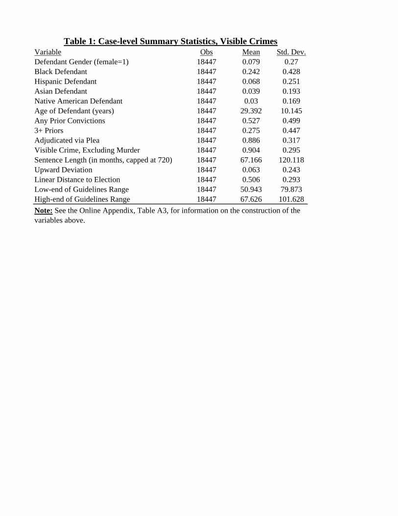
Variable Obs Mean Std. Dev.Defendant Gender (female=1) 18447 0.079 0.27Black Defendant 18447 0.242 0.428Hispanic Defendant 18447 0.068 0.251Asian Defendant 18447 0.039 0.193Native American Defendant 18447 0.03 0.169Age of Defendant (years) 18447 29.392 10.145Any Prior Convictions 18447 0.527 0.4993+ Priors 18447 0.275 0.447Adjudicated via Plea 18447 0.886 0.317Visible Crime, Excluding Murder 18447 0.904 0.295Sentence Length (in months, capped at 720) 18447 67.166 120.118Upward Deviation 18447 0.063 0.243Linear Distance to Election 18447 0.506 0.293Low-end of Guidelines Range 18447 50.943 79.873High-end of Guidelines Range 18447 67.626 101.628

Table 1: Case-level Summary Statistics, Visible Crimes

Note: See the Online Appendix, Table A3, for information on the construction of the variables above.

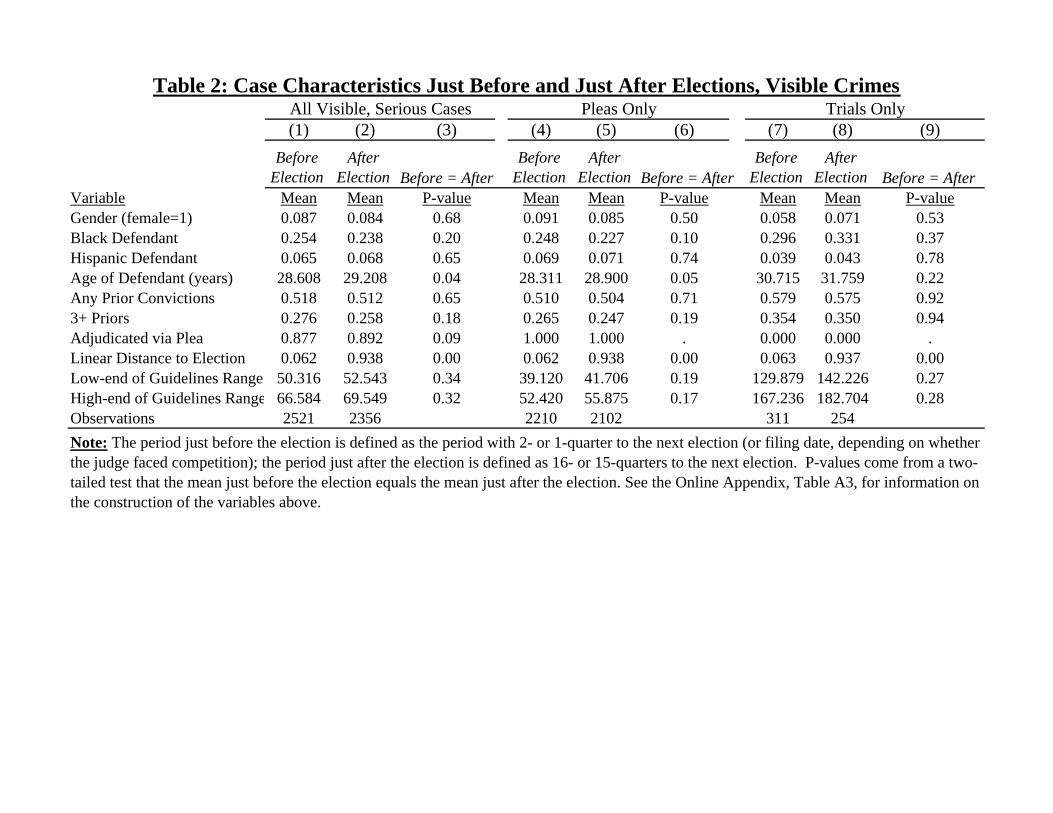
(1) (2) (3) (4) (5) (6) (7) (8) (9)Before

ElectionAfter

Election Before = AfterBefore

ElectionAfter

Election Before = AfterBefore

ElectionAfter

Election Before = AfterVariable Mean Mean P-value Mean Mean P-value Mean Mean P-valueGender (female=1) 0.087 0.084 0.68 0.091 0.085 0.50 0.058 0.071 0.53Black Defendant 0.254 0.238 0.20 0.248 0.227 0.10 0.296 0.331 0.37Hispanic Defendant 0.065 0.068 0.65 0.069 0.071 0.74 0.039 0.043 0.78Age of Defendant (years) 28.608 29.208 0.04 28.311 28.900 0.05 30.715 31.759 0.22Any Prior Convictions 0.518 0.512 0.65 0.510 0.504 0.71 0.579 0.575 0.923+ Priors 0.276 0.258 0.18 0.265 0.247 0.19 0.354 0.350 0.94Adjudicated via Plea 0.877 0.892 0.09 1.000 1.000 . 0.000 0.000 .Linear Distance to Election 0.062 0.938 0.00 0.062 0.938 0.00 0.063 0.937 0.00Low-end of Guidelines Range 50.316 52.543 0.34 39.120 41.706 0.19 129.879 142.226 0.27High-end of Guidelines Range 66.584 69.549 0.32 52.420 55.875 0.17 167.236 182.704 0.28Observations 2521 2356 2210 2102 311 254Note: The period just before the election is defined as the period with 2- or 1-quarter to the next election (or filing date, depending on whether the judge faced competition); the period just after the election is defined as 16- or 15-quarters to the next election. P-values come from a two-tailed test that the mean just before the election equals the mean just after the election. See the Online Appendix, Table A3, for information on the construction of the variables above.

Pleas Only Trials OnlyTable 2: Case Characteristics Just Before and Just After Elections, Visible Crimes

All Visible, Serious Cases

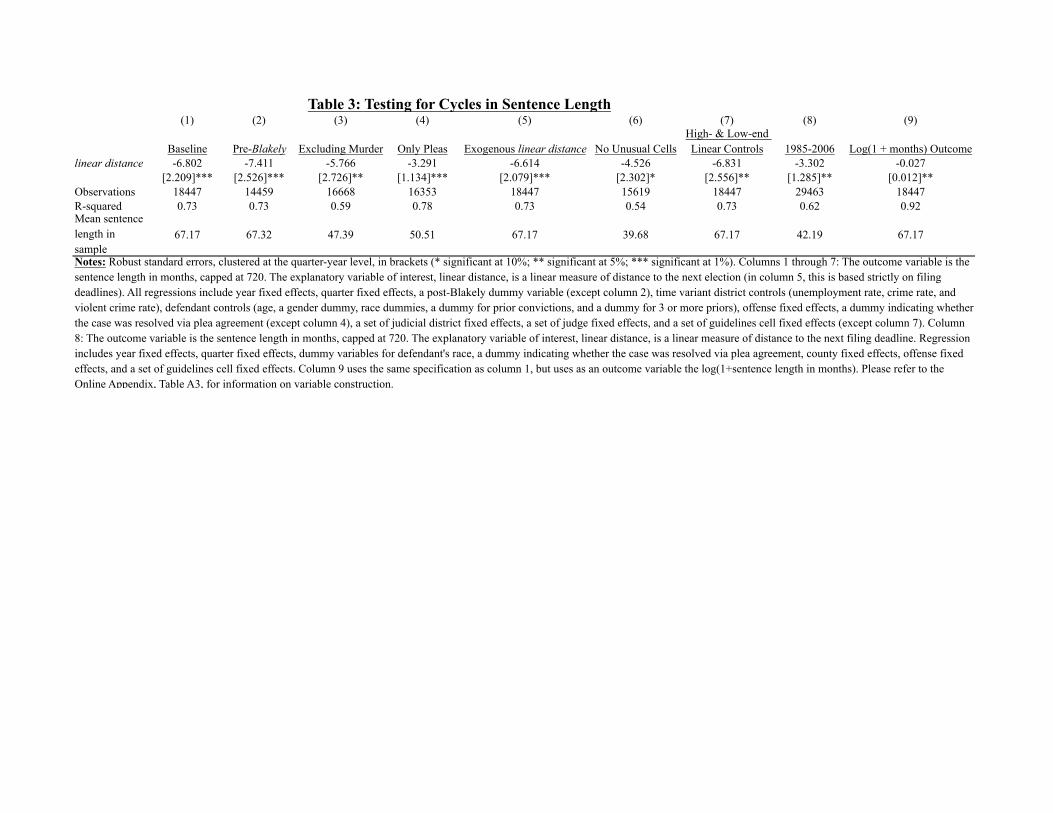
(1) (2) (3) (4) (5) (6) (7) (8) (9)

Baseline Pre-Blakely Excluding Murder Only Pleas Exogenous linear distance No Unusual CellsHigh- & Low-end Linear Controls 1985-2006 Log(1 + months) Outcome

linear distance -6.802 -7.411 -5.766 -3.291 -6.614 -4.526 -6.831 -3.302 -0.027[2.209]*** [2.526]*** [2.726]** [1.134]*** [2.079]*** [2.302]* [2.556]** [1.285]** [0.012]**

Observations 18447 14459 16668 16353 18447 15619 18447 29463 18447R-squared 0.73 0.73 0.59 0.78 0.73 0.54 0.73 0.62 0.92Mean sentence length in sample

67.17 67.32 47.39 50.51 67.17 39.68 67.17 42.19 67.17

Table 3: Testing for Cycles in Sentence Length

Notes: Robust standard errors, clustered at the quarter-year level, in brackets (* significant at 10%; ** significant at 5%; *** significant at 1%). Columns 1 through 7: The outcome variable is the sentence length in months, capped at 720. The explanatory variable of interest, linear distance, is a linear measure of distance to the next election (in column 5, this is based strictly on filing deadlines). All regressions include year fixed effects, quarter fixed effects, a post-Blakely dummy variable (except column 2), time variant district controls (unemployment rate, crime rate, and violent crime rate), defendant controls (age, a gender dummy, race dummies, a dummy for prior convictions, and a dummy for 3 or more priors), offense fixed effects, a dummy indicating whether the case was resolved via plea agreement (except column 4), a set of judicial district fixed effects, a set of judge fixed effects, and a set of guidelines cell fixed effects (except column 7). Column 8: The outcome variable is the sentence length in months, capped at 720. The explanatory variable of interest, linear distance, is a linear measure of distance to the next filing deadline. Regression includes year fixed effects, quarter fixed effects, dummy variables for defendant's race, a dummy indicating whether the case was resolved via plea agreement, county fixed effects, offense fixed effects, and a set of guidelines cell fixed effects. Column 9 uses the same specification as column 1, but uses as an outcome variable the log(1+sentence length in months). Please refer to the Online Appendix, Table A3, for information on variable construction.

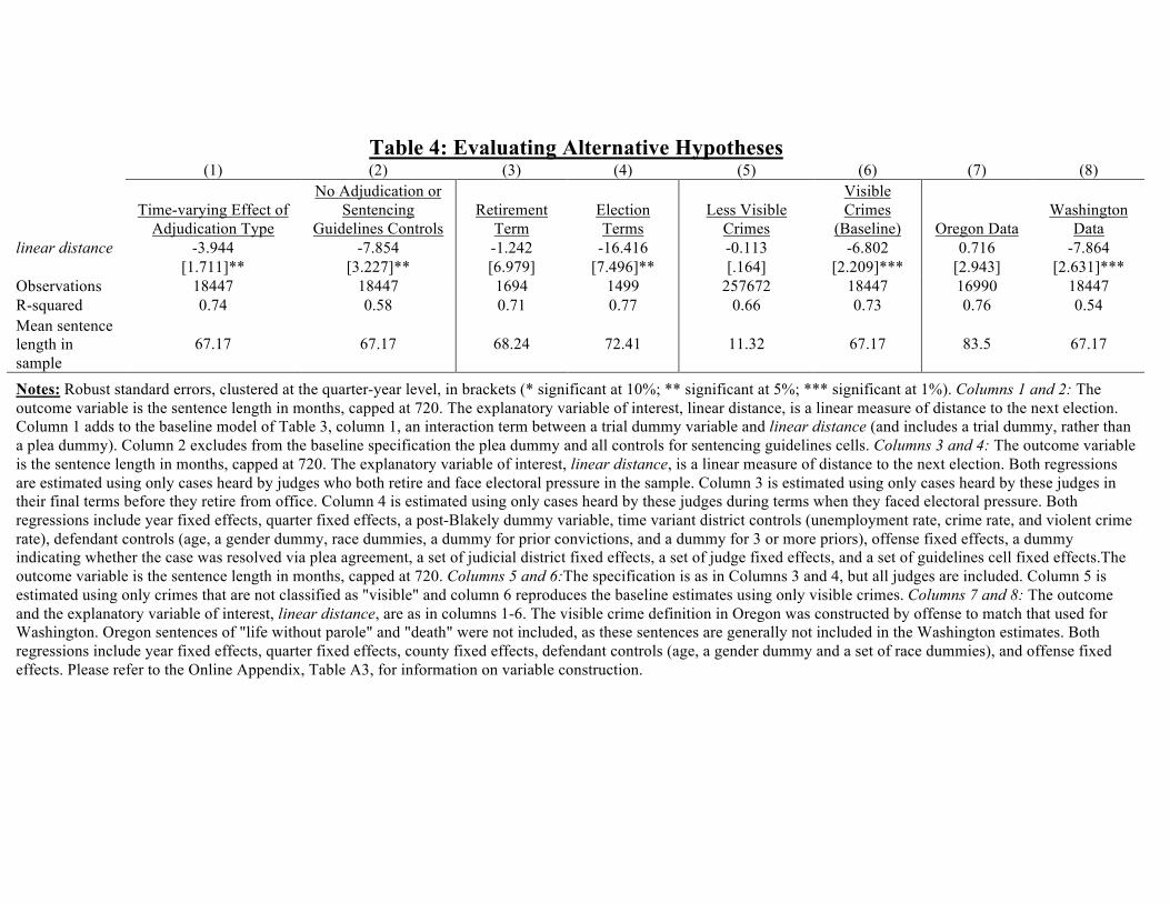
Table 4: Evaluating Alternative Hypotheses (1) (2) (3) (4) (5) (6) (7) (8)

Time-varying Effect of

Adjudication Type

No Adjudication or Sentencing

Guidelines Controls Retirement

Term Election Terms

Less Visible Crimes

Visible Crimes

(Baseline) Oregon Data Washington

Data linear distance -3.944 -7.854 -1.242 -16.416 -0.113 -6.802 0.716 -7.864 [1.711]** [3.227]** [6.979] [7.496]** [.164] [2.209]*** [2.943] [2.631]*** Observations 18447 18447 1694 1499 257672 18447 16990 18447 R-squared 0.74 0.58 0.71 0.77 0.66 0.73 0.76 0.54 Mean sentence length in sample

67.17 67.17 68.24 72.41 11.32 67.17 83.5 67.17

Notes: Robust standard errors, clustered at the quarter-year level, in brackets (* significant at 10%; ** significant at 5%; *** significant at 1%). Columns 1 and 2: The outcome variable is the sentence length in months, capped at 720. The explanatory variable of interest, linear distance, is a linear measure of distance to the next election. Column 1 adds to the baseline model of Table 3, column 1, an interaction term between a trial dummy variable and linear distance (and includes a trial dummy, rather than a plea dummy). Column 2 excludes from the baseline specification the plea dummy and all controls for sentencing guidelines cells. Columns 3 and 4: The outcome variable is the sentence length in months, capped at 720. The explanatory variable of interest, linear distance, is a linear measure of distance to the next election. Both regressions are estimated using only cases heard by judges who both retire and face electoral pressure in the sample. Column 3 is estimated using only cases heard by these judges in their final terms before they retire from office. Column 4 is estimated using only cases heard by these judges during terms when they faced electoral pressure. Both regressions include year fixed effects, quarter fixed effects, a post-Blakely dummy variable, time variant district controls (unemployment rate, crime rate, and violent crime rate), defendant controls (age, a gender dummy, race dummies, a dummy for prior convictions, and a dummy for 3 or more priors), offense fixed effects, a dummy indicating whether the case was resolved via plea agreement, a set of judicial district fixed effects, a set of judge fixed effects, and a set of guidelines cell fixed effects.The outcome variable is the sentence length in months, capped at 720. Columns 5 and 6:The specification is as in Columns 3 and 4, but all judges are included. Column 5 is estimated using only crimes that are not classified as "visible" and column 6 reproduces the baseline estimates using only visible crimes. Columns 7 and 8: The outcome and the explanatory variable of interest, linear distance, are as in columns 1-6. The visible crime definition in Oregon was constructed by offense to match that used for Washington. Oregon sentences of "life without parole" and "death" were not included, as these sentences are generally not included in the Washington estimates. Both regressions include year fixed effects, quarter fixed effects, county fixed effects, defendant controls (age, a gender dummy and a set of race dummies), and offense fixed effects. Please refer to the Online Appendix, Table A3, for information on variable construction.

 

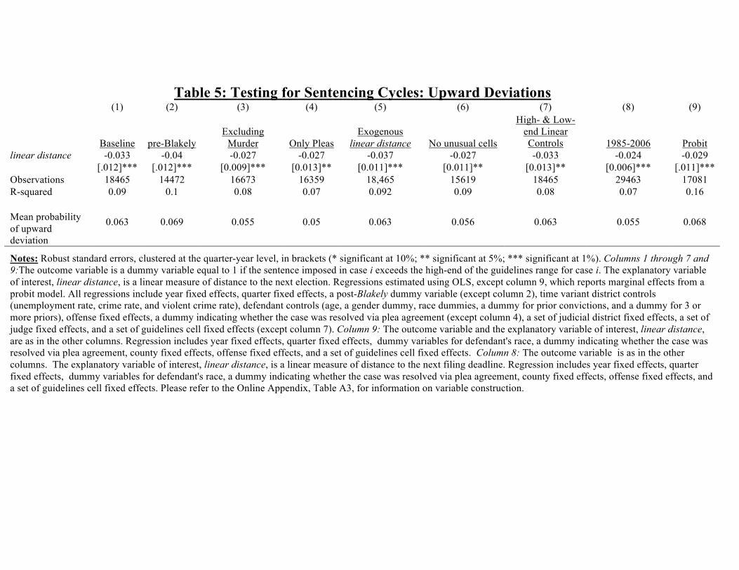
Table 5: Testing for Sentencing Cycles: Upward Deviations (1) (2) (3) (4) (5) (6) (7) (8) (9)

Baseline pre-Blakely Excluding

Murder Only Pleas Exogenous

linear distance No unusual cells

High- & Low-end Linear Controls 1985-2006 Probit

linear distance -0.033 -0.04 -0.027 -0.027 -0.037 -0.027 -0.033 -0.024 -0.029 [.012]*** [.012]*** [0.009]*** [0.013]** [0.011]*** [0.011]** [0.013]** [0.006]*** [.011]*** Observations 18465 14472 16673 16359 18,465 15619 18465 29463 17081 R-squared 0.09 0.1 0.08 0.07 0.092 0.09 0.08 0.07 0.16

Mean probability of upward deviation

0.063 0.069 0.055 0.05 0.063 0.056 0.063 0.055 0.068

Notes: Robust standard errors, clustered at the quarter-year level, in brackets (* significant at 10%; ** significant at 5%; *** significant at 1%). Columns 1 through 7 and 9:The outcome variable is a dummy variable equal to 1 if the sentence imposed in case i exceeds the high-end of the guidelines range for case i. The explanatory variable of interest, linear distance, is a linear measure of distance to the next election. Regressions estimated using OLS, except column 9, which reports marginal effects from a probit model. All regressions include year fixed effects, quarter fixed effects, a post-Blakely dummy variable (except column 2), time variant district controls (unemployment rate, crime rate, and violent crime rate), defendant controls (age, a gender dummy, race dummies, a dummy for prior convictions, and a dummy for 3 or more priors), offense fixed effects, a dummy indicating whether the case was resolved via plea agreement (except column 4), a set of judicial district fixed effects, a set of judge fixed effects, and a set of guidelines cell fixed effects (except column 7). Column 9: The outcome variable and the explanatory variable of interest, linear distance, are as in the other columns. Regression includes year fixed effects, quarter fixed effects, dummy variables for defendant's race, a dummy indicating whether the case was resolved via plea agreement, county fixed effects, offense fixed effects, and a set of guidelines cell fixed effects. Column 8: The outcome variable is as in the other columns. The explanatory variable of interest, linear distance, is a linear measure of distance to the next filing deadline. Regression includes year fixed effects, quarter fixed effects, dummy variables for defendant's race, a dummy indicating whether the case was resolved via plea agreement, county fixed effects, offense fixed effects, and a set of guidelines cell fixed effects. Please refer to the Online Appendix, Table A3, for information on variable construction.

 

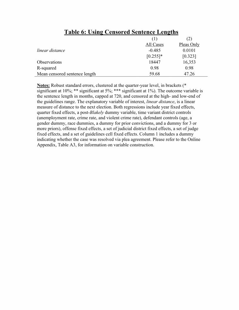
Table 6: Using Censored Sentence Lengths (1) (2)

All Cases Pleas Only linear distance -0.485 0.0101 [0.255]* [0.323] Observations 18447 16,353 R-squared 0.98 0.98 Mean censored sentence length 59.68 47.26

Notes: Robust standard errors, clustered at the quarter-year level, in brackets (* significant at 10%; ** significant at 5%; *** significant at 1%). The outcome variable is the sentence length in months, capped at 720, and censored at the high- and low-end of the guidelines range. The explanatory variable of interest, linear distance, is a linear measure of distance to the next election. Both regressions include year fixed effects, quarter fixed effects, a post-Blakely dummy variable, time variant district controls (unemployment rate, crime rate, and violent crime rate), defendant controls (age, a gender dummy, race dummies, a dummy for prior convictions, and a dummy for 3 or more priors), offense fixed effects, a set of judicial district fixed effects, a set of judge fixed effects, and a set of guidelines cell fixed effects. Column 1 includes a dummy indicating whether the case was resolved via plea agreement. Please refer to the Online Appendix, Table A3, for information on variable construction.

 

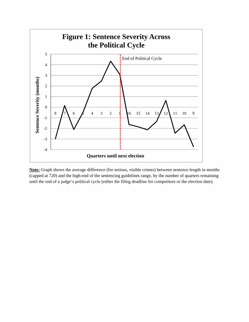
Note: Graph shows the average difference (for serious, visible crimes) between sentence length in months (capped at 720) and the high-end of the sentencing guidelines range, by the number of quarters remaining until the end of a judge’s political cycle (either the filing deadline for competitors or the election date).

-4

-3

-2

-1

0

1

2

3

4

5

8 7 6 5 4 3 2 1 16 15 14 13 12 11 10 9

Sent

ence

Sev

erity

(mon

ths)

Figure 1: Sentence Severity Acrossthe Political Cycle

End of Political Cycle

Quarters until next election

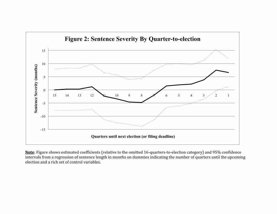
   Note:  Figure  shows  estimated  coefficients  (relative  to  the  omitted  16-­‐quarters-­‐to-­‐election  category)  and  95%  confidence  intervals  from  a  regression  of  sentence  length  in  months  on  dummies  indicating  the  number  of  quarters  until  the  upcoming  election  and  a  rich  set  of  control  variables.  

-15

-10

-5

0

5

10

15

15 14 13 12 11 10 9 8 7 6 5 4 3 2 1

Sent

ence

Sev

erity

(mon

ths)

Figure 2: Sentence Severity By Quarter-to-election

Quarters until next election (or filing deadline)

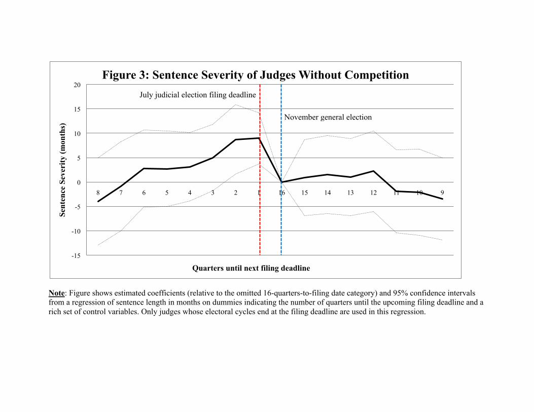
   Note: Figure shows estimated coefficients (relative to the omitted 16-quarters-to-filing date category) and 95% confidence intervals from a regression of sentence length in months on dummies indicating the number of quarters until the upcoming filing deadline and a rich set of control variables. Only judges whose electoral cycles end at the filing deadline are used in this regression.

-15

-10

-5

0

5

10

15

20

8 7 6 5 4 3 2 1 16 15 14 13 12 11 10 9

Sent

ence

Sev

erity

(mon

ths)

Figure 3: Sentence Severity of Judges Without Competition

Quarters until next filing deadline

July judicial election filing deadline

November general election

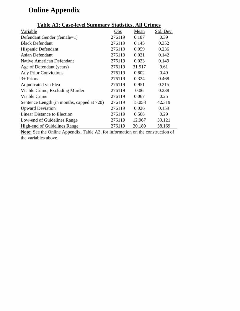
Variable Obs Mean Std. Dev.Defendant Gender (female=1) 276119 0.187 0.39Black Defendant 276119 0.145 0.352Hispanic Defendant 276119 0.059 0.236Asian Defendant 276119 0.021 0.142Native American Defendant 276119 0.023 0.149Age of Defendant (years) 276119 31.517 9.61Any Prior Convictions 276119 0.602 0.493+ Priors 276119 0.324 0.468Adjudicated via Plea 276119 0.951 0.215Visible Crime, Excluding Murder 276119 0.06 0.238Visible Crime 276119 0.067 0.25Sentence Length (in months, capped at 720) 276119 15.053 42.319Upward Deviation 276119 0.026 0.159Linear Distance to Election 276119 0.508 0.29Low-end of Guidelines Range 276119 12.967 30.121High-end of Guidelines Range 276119 20.189 38.169

Table A1: Case-level Summary Statistics, All Crimes

Note: See the Online Appendix, Table A3, for information on the construction of the variables above.

Online Appendix

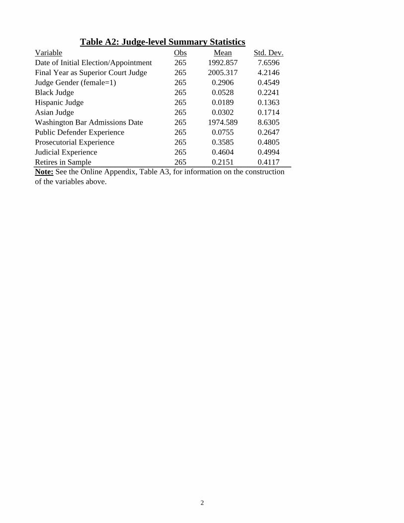
Variable Obs Mean Std. Dev.Date of Initial Election/Appointment 265 1992.857 7.6596Final Year as Superior Court Judge 265 2005.317 4.2146Judge Gender (female=1) 265 0.2906 0.4549Black Judge 265 0.0528 0.2241Hispanic Judge 265 0.0189 0.1363Asian Judge 265 0.0302 0.1714Washington Bar Admissions Date 265 1974.589 8.6305Public Defender Experience 265 0.0755 0.2647Prosecutorial Experience 265 0.3585 0.4805Judicial Experience 265 0.4604 0.4994Retires in Sample 265 0.2151 0.4117

Table A2: Judge-level Summary Statistics

Note: See the Online Appendix, Table A3, for information on the construction of the variables above.

2

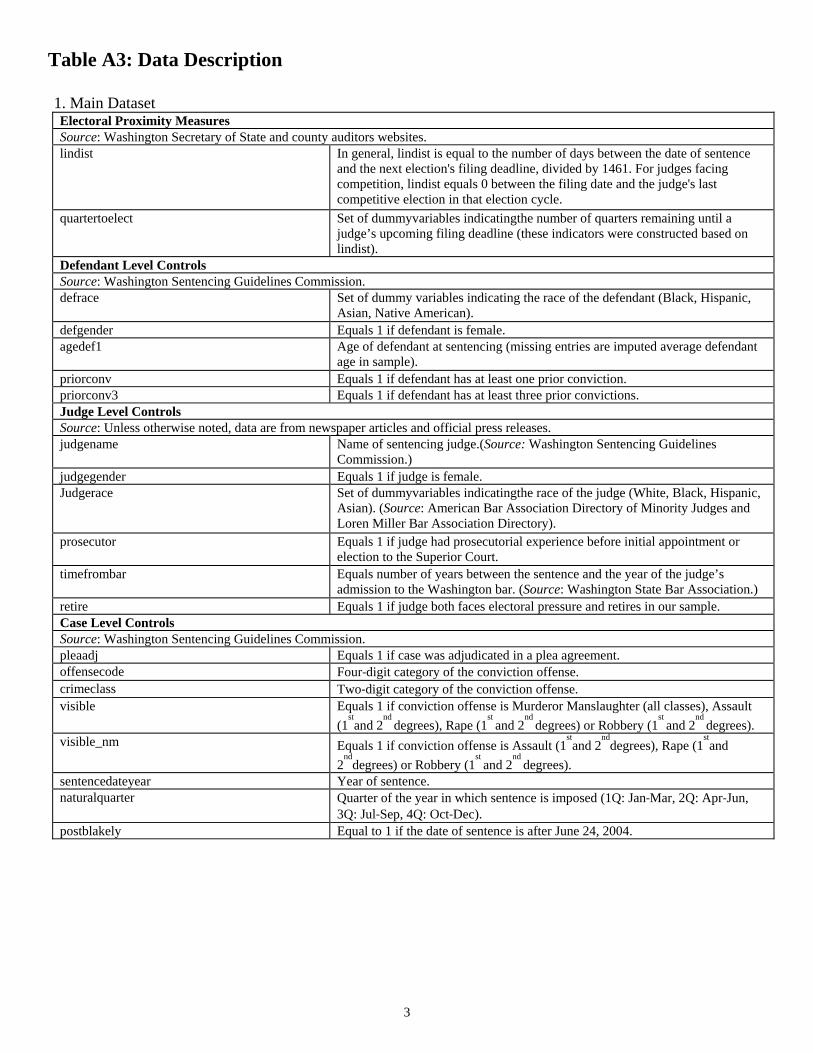
Table A3: Data Description 1. Main Dataset Electoral Proximity Measures Source: Washington Secretary of State and county auditors websites. lindist In general, lindist is equal to the number of days between the date of sentence

and the next election's filing deadline, divided by 1461. For judges facing competition, lindist equals 0 between the filing date and the judge's last competitive election in that election cycle.

quartertoelect Set of dummyvariables indicatingthe number of quarters remaining until a judge’s upcoming filing deadline (these indicators were constructed based on lindist).

Defendant Level Controls Source: Washington Sentencing Guidelines Commission. defrace Set of dummy variables indicating the race of the defendant (Black, Hispanic,

Asian, Native American). defgender Equals 1 if defendant is female. agedef1 Age of defendant at sentencing (missing entries are imputed average defendant

age in sample). priorconv Equals 1 if defendant has at least one prior conviction. priorconv3 Equals 1 if defendant has at least three prior convictions. Judge Level Controls Source: Unless otherwise noted, data are from newspaper articles and official press releases. judgename Name of sentencing judge.(Source: Washington Sentencing Guidelines

Commission.) judgegender Equals 1 if judge is female. Judgerace Set of dummyvariables indicatingthe race of the judge (White, Black, Hispanic,

Asian). (Source: American Bar Association Directory of Minority Judges and Loren Miller Bar Association Directory).

prosecutor Equals 1 if judge had prosecutorial experience before initial appointment or election to the Superior Court.

timefrombar Equals number of years between the sentence and the year of the judge’s admission to the Washington bar. (Source: Washington State Bar Association.)

retire Equals 1 if judge both faces electoral pressure and retires in our sample. Case Level Controls Source: Washington Sentencing Guidelines Commission. pleaadj Equals 1 if case was adjudicated in a plea agreement. offensecode Four‐digit category of the conviction offense. crimeclass Two‐digit category of the conviction offense. visible Equals 1 if conviction offense is Murderor Manslaughter (all classes), Assault

(1stand 2

nd degrees), Rape (1

st and 2

nd degrees) or Robbery (1

st and 2

nd degrees).

visible_nm Equals 1 if conviction offense is Assault (1stand 2

nddegrees), Rape (1

stand

2nd

degrees) or Robbery (1st

and 2nd

degrees). sentencedateyear Year of sentence. naturalquarter Quarter of the year in which sentence is imposed (1Q: Jan‐Mar, 2Q: Apr‐Jun,

3Q: Jul‐Sep, 4Q: Oct‐Dec). postblakely Equal to 1 if the date of sentence is after June 24, 2004.

3

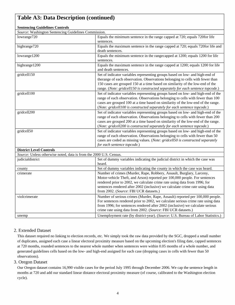
Table A3: Data Description (continued) Sentencing Guidelines Controls Source: Washington Sentencing Guidelines Commission. lowrange720 Equals the minimum sentence in the range capped at 720; equals 720for life

sentences. highrange720 Equals the maximum sentence in the range capped at 720; equals 720for life and

death sentences. lowrange1200 Equals the minimum sentence in the rangecapped at 1200; equals 1200 for life

sentences. highrange1200 Equals the maximum sentence in the range capped at 1200; equals 1200 for life

and death sentences. gridcell150 Set of indicator variables representing groups based on low‐ and high‐end of

therange of each observation. Observations belonging to cells with fewer than 150 cases are grouped 150 at a time based on similarity of the low‐end of the range. (Note: gridcell150 is constructed separately for each sentence topcode.)

gridcell100 Set of indicator variables representing groups based on low‐ and high‐end of the range of each observation. Observations belonging to cells with fewer than 100 cases are grouped 100 at a time based on similarity of the low‐end of the range. (Note: gridcell100 is constructed separately for each sentence topcode.)

gridcell200 Set of indicator variables representing groups based on low‐ and high‐end of the range of each observation. Observations belonging to cells with fewer than 200 cases are grouped 200 at a time based on similarity of the low‐end of the range. (Note: gridcell200 is constructed separately for each sentence topcode.)

gridcell50 Set of indicator variables representing groups based on low‐ and high‐end of the range of each observation. Observations belonging to cells with fewer than 50 cases are coded as missing values. (Note: gridcell50 is constructed separately for each sentence topcode.)

District Level Controls Source: Unless otherwise noted, data is from the 2000 U.S. Census. judicialdistrict Set of dummy variables indicating the judicial district in which the case was

heard. county Set of dummy variables indicating the county in which the case was heard. crimerate Number of crimes (Murder, Rape, Robbery, Assault, Burglary, Larceny,

Motor‐vehicle Theft, and Arson) reported per 100,000 people. For sentences rendered prior to 2002, we calculate crime rate using data from 1996; for sentences rendered after 2002 (inclusive) we calculate crime rate using data from 2002. (Source: FBI UCR datasets.)

violcrimerate Number of serious crimes (Murder, Rape, Assault) reported per 100,000 people. For sentences rendered prior to 2002, we calculate serious crime rate using data from 1996; for sentences rendered after 2002 (inclusive) we calculate serious crime rate using data from 2002. (Source: FBI UCR datasets.)

unemp Unemployment rate (by district‐year). (Source: U.S. Bureau of Labor Statistics.)

2. Extended Dataset This dataset required no linking to election records, etc. We simply took the raw data provided by the SGC, dropped a small number of duplicates, assigned each case a linear electoral proximity measure based on the upcoming election's filing date, capped sentences at 720 months, rounded sentences to the nearest whole number when sentences were within 0.05 months of a whole number, and generated guidelines cells based on the low- and high-end assigned for each case (dropping cases in cells with fewer than 50 observations).

3. Oregon Dataset Our Oregon dataset contains 16,990 visible cases for the period July 1995 through December 2006. We cap the sentence length in months at 720 and add our standard linear distance electoral proximity measure (of course, calibrated to the Washington election cycle).

4

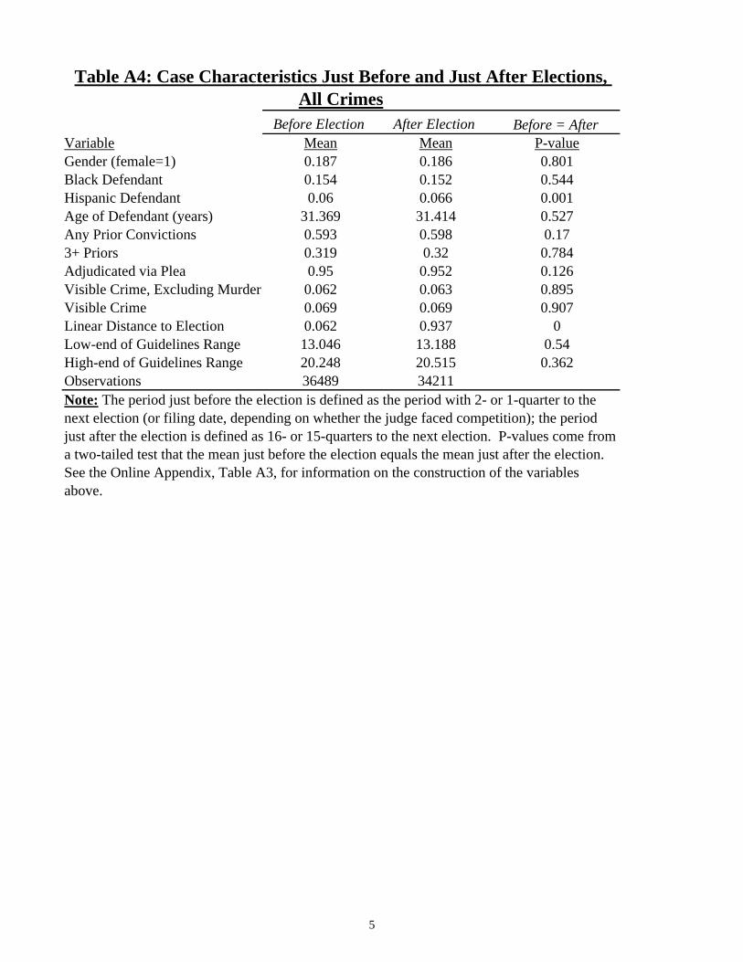
Before Election After Election Before = AfterVariable Mean Mean P-valueGender (female=1) 0.187 0.186 0.801Black Defendant 0.154 0.152 0.544Hispanic Defendant 0.06 0.066 0.001Age of Defendant (years) 31.369 31.414 0.527Any Prior Convictions 0.593 0.598 0.173+ Priors 0.319 0.32 0.784Adjudicated via Plea 0.95 0.952 0.126Visible Crime, Excluding Murder 0.062 0.063 0.895Visible Crime 0.069 0.069 0.907Linear Distance to Election 0.062 0.937 0Low-end of Guidelines Range 13.046 13.188 0.54High-end of Guidelines Range 20.248 20.515 0.362Observations 36489 34211

Table A4: Case Characteristics Just Before and Just After Elections, All Crimes

Note: The period just before the election is defined as the period with 2- or 1-quarter to the next election (or filing date, depending on whether the judge faced competition); the period just after the election is defined as 16- or 15-quarters to the next election. P-values come from a two-tailed test that the mean just before the election equals the mean just after the election. See the Online Appendix, Table A3, for information on the construction of the variables above.

5

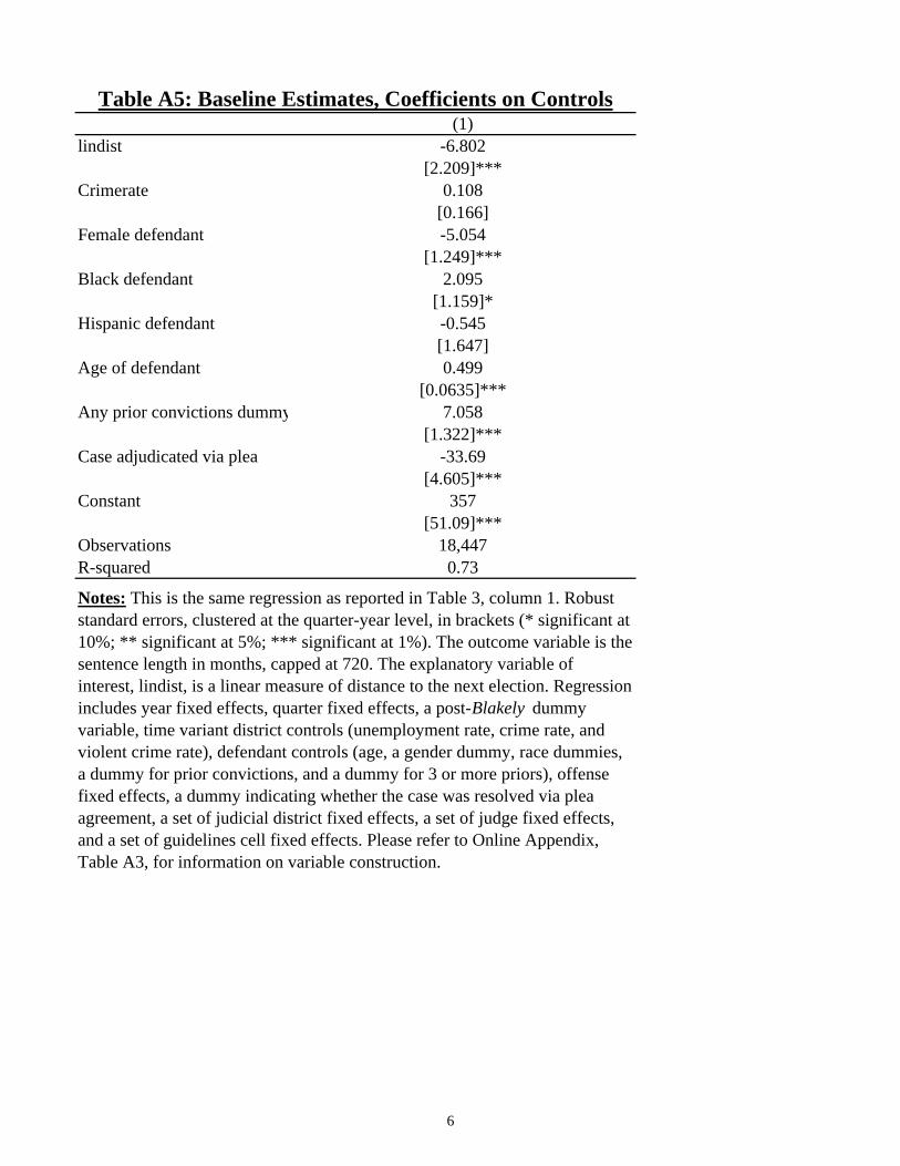
(1)lindist -6.802

[2.209]***Crimerate 0.108

[0.166]Female defendant -5.054

[1.249]***Black defendant 2.095

[1.159]*Hispanic defendant -0.545

[1.647]Age of defendant 0.499

[0.0635]***Any prior convictions dummy 7.058

[1.322]***Case adjudicated via plea -33.69

[4.605]***Constant 357

[51.09]***Observations 18,447R-squared 0.73

Table A5: Baseline Estimates, Coefficients on Controls

Notes: This is the same regression as reported in Table 3, column 1. Robust standard errors, clustered at the quarter-year level, in brackets (* significant at 10%; ** significant at 5%; *** significant at 1%). The outcome variable is the sentence length in months, capped at 720. The explanatory variable of interest, lindist, is a linear measure of distance to the next election. Regression includes year fixed effects, quarter fixed effects, a post-Blakely dummy variable, time variant district controls (unemployment rate, crime rate, and violent crime rate), defendant controls (age, a gender dummy, race dummies, a dummy for prior convictions, and a dummy for 3 or more priors), offense fixed effects, a dummy indicating whether the case was resolved via plea agreement, a set of judicial district fixed effects, a set of judge fixed effects, and a set of guidelines cell fixed effects. Please refer to Online Appendix, Table A3, for information on variable construction.

6

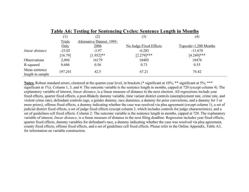
Table A6: Testing for Sentencing Cycles: Sentence Length in Months (1) (2) (3) (4)

Trials Only

Alternative Dataset, 1995-2006 No Judge Fixed Effects Topcode=1,200 Months

linear distance -23.02 -3.97 -6.283 -11.678 [16.79] [1.952]** [2.279]*** [4.249]*** Observations 2,094 16179 18405 18476 R-squared 0.686 0.56 0.73 0.55 Mean sentence length in sample

197.241 42.5 67.21 74.42

Notes: Robust standard errors, clustered at the quarter-year level, in brackets (* significant at 10%; ** significant at 5%; *** significant at 1%). Column 1, 3, and 4: The outcome variable is the sentence length in months, capped at 720 (except column 4). The explanatory variable of interest, linear distance, is a linear measure of distance to the next election. All regressions include year fixed effects, quarter fixed effects, a post-Blakely dummy variable, time variant district controls (unemployment rate, crime rate, and violent crime rate), defendant controls (age, a gender dummy, race dummies, a dummy for prior convictions, and a dummy for 3 or more priors), offense fixed effects, a dummy indicating whether the case was resolved via plea agreement (except column 1), a set of judicial district fixed effects, a set of judge fixed effects (except column 3, which includes controls for judge characteristics), and a set of guidelines cell fixed effects. Column 2: The outcome variable is the sentence length in months, capped at 720. The explanatory variable of interest, linear distance, is a linear measure of distance to the next filing deadline. Regression includes year fixed effects, quarter fixed effects, dummy variables for defendant's race, a dummy indicating whether the case was resolved via plea agreement, county fixed effects, offense fixed effects, and a set of guidelines cell fixed effects. Please refer to the Online Appendix, Table A3, for information on variable construction.

 

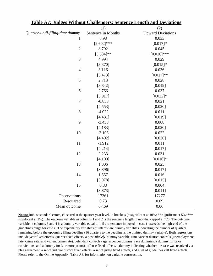
(1) (2)Quarter-until-filing-date dummy Sentence in Months Upward Deviations

1 8.98 0.033[2.602]*** [0.017]*

2 8.702 0.045[3.534]** [0.016]***

3 4.994 0.029[3.370] [0.015]*

4 3.116 0.036[3.473] [0.017]**

5 2.713 0.028[3.842] [0.019]

6 2.766 0.037[3.917] [0.022]*

7 -0.858 0.021[4.553] [0.020]

8 -4.022 0.011[4.431] [0.019]

9 -3.458 0.008[4.183] [0.020]

10 -2.103 0.022[4.402] [0.020]

11 -1.912 0.011[4.214] [0.017]

12 2.233 0.031[4.100] [0.016]*

13 1.006 0.025[3.896] [0.017]

14 1.557 0.016[3.978] [0.015]

15 0.88 0.004[3.873] [0.011]

Observations 17261 17277R-squared 0.73 0.09

Mean outcome 67.69 0.06

Table A7: Judges Without Challengers: Sentence Length and Deviations

Notes: Robust standard errors, clustered at the quarter-year level, in brackets (* significant at 10%; ** significant at 5%; *** significant at 1%). The outcome variable in columns 1 and 2 is the sentence length in months, capped at 720. The outcome variable in columns 3 and 4 is a dummy variable equal to 1 if the sentence imposed in case i exceeds the high-end of the guidelines range for case i . The explanatory variables of interest are dummy variables indicating the number of quarters remaining before the upcoming filing deadline (16 quarters to the deadline is the omitted dummy variable). Both regressions include year fixed effects, quarter fixed effects, a post-Blakely dummy variable, time variant district controls (unemployment rate, crime rate, and violent crime rate), defendant controls (age, a gender dummy, race dummies, a dummy for prior convictions, and a dummy for 3 or more priors), offense fixed effects, a dummy indicating whether the case was resolved via plea agreement, a set of judicial district fixed effects, a set of judge fixed effects, and a set of guidelines cell fixed effects. Please refer to the Online Appendix, Table A3, for information on variable construction.

8

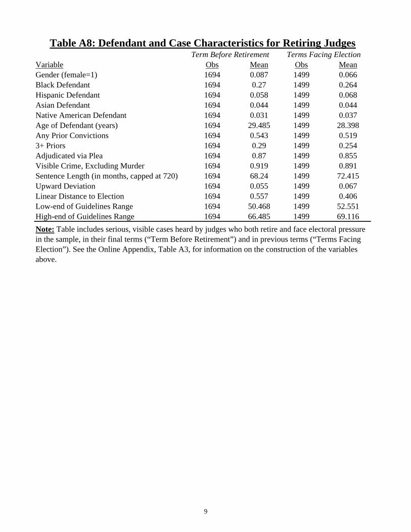
Variable Obs Mean Obs MeanGender (female=1) 1694 0.087 1499 0.066Black Defendant 1694 0.27 1499 0.264Hispanic Defendant 1694 0.058 1499 0.068

Table A8: Defendant and Case Characteristics for Retiring JudgesTerm Before Retirement Terms Facing Election

spa c e e da t 69 0.058 99 0.068Asian Defendant 1694 0.044 1499 0.044Native American Defendant 1694 0.031 1499 0.037Age of Defendant (years) 1694 29.485 1499 28.398Any Prior Convictions 1694 0.543 1499 0.5193+ Priors 1694 0.29 1499 0.254Adjudicated via Plea 1694 0.87 1499 0.855jVisible Crime, Excluding Murder 1694 0.919 1499 0.891Sentence Length (in months, capped at 720) 1694 68.24 1499 72.415Upward Deviation 1694 0.055 1499 0.067Linear Distance to Election 1694 0.557 1499 0.406Low-end of Guidelines Range 1694 50.468 1499 52.551High-end of Guidelines Range 1694 66.485 1499 69.116Note: Table includes serious, visible cases heard by judges who both retire and face electoral pressure in the sample, in their final terms (“Term Before Retirement”) and in previous terms (“Terms Facing Election”). See the Online Appendix, Table A3, for information on the construction of the variables above.

9

(1)All Visible Crimes

Visible dummy 15.57[1.678]***

lindist -0.192[0.225]

lindist*Visible -4.89[2.188]**

Observations 276119R-squared 0.72Mean sentence length 15.05

Table A9: Sentencing Cycles for Visible and Less-Visible Crimes

Notes: Robust standard errors, clustered at the quarter-year level, in brackets (* significant at 10%; ** significant at 5%; *** significant at 1%). The outcome variable is the sentence length in months, capped at 720. The explanatory variables of interest are a visible crimes dummy variable (equal to 1 if case i involved a visible crime), lindist (a linear measure of distance to the next election), and the interaction between the visible crimes dummy and lindist. Regression includes year fixed effects, quarter fixed effects, a post-Blakely dummy variable, time variant district controls (unemployment rate, crime rate, and violent crime rate), defendant controls (age, a gender dummy, race dummies, a dummy for prior convictions, and a dummy for 3 or more priors), offense fixed effects, a dummy indicating whether the case was resolved via plea agreement, a set of judicial district fixed effects, a set of judge fixed effects, and a set of guidelines cell fixed effects. Please refer to the Online Appendix, Table A3, for information on variable construction.

10

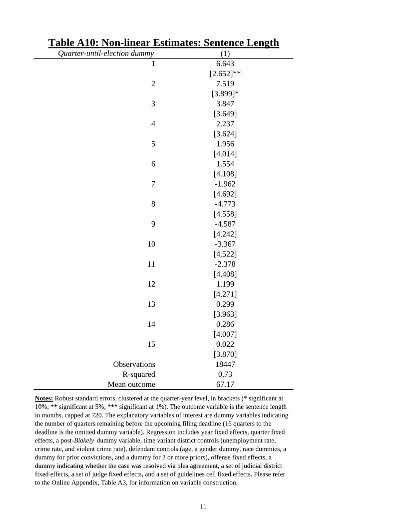
Quarter-until-election dummy (1)1 6.643

[2.652]**2 7.519

[3.899]*

Table A10: Non-linear Estimates: Sentence Length

[ ]3 3.847

[3.649]4 2.237

[3.624]5 1.956

[4.014]6 1.554

[4.108]7 -1.962

[4.692]8 -4.773

[4.558]9 4 89 -4.587

[4.242]10 -3.367

[4.522]11 -2.378

[4.408]12 1 19912 1.199

[4.271]13 0.299

[3.963]14 0.286

[4.007]15 0 02215 0.022

[3.870]Observations 18447

R-squared 0.73Mean outcome 67.17

Notes: Robust standard errors, clustered at the quarter-year level, in brackets (* significant at 10%; ** significant at 5%; *** significant at 1%) The outcome variable is the sentence length10%; ** significant at 5%; *** significant at 1%). The outcome variable is the sentence length in months, capped at 720. The explanatory variables of interest are dummy variables indicating the number of quarters remaining before the upcoming filing deadline (16 quarters to the deadline is the omitted dummy variable). Regression includes year fixed effects, quarter fixed effects, a post-Blakely dummy variable, time variant district controls (unemployment rate, crime rate, and violent crime rate), defendant controls (age, a gender dummy, race dummies, a dummy for prior convictions, and a dummy for 3 or more priors), offense fixed effects, a dummy indicating whether the case was resolved via plea agreement, a set of judicial districtdummy indicating whether the case was resolved via plea agreement, a set of judicial district fixed effects, a set of judge fixed effects, and a set of guidelines cell fixed effects. Please refer to the Online Appendix, Table A3, for information on variable construction.

11

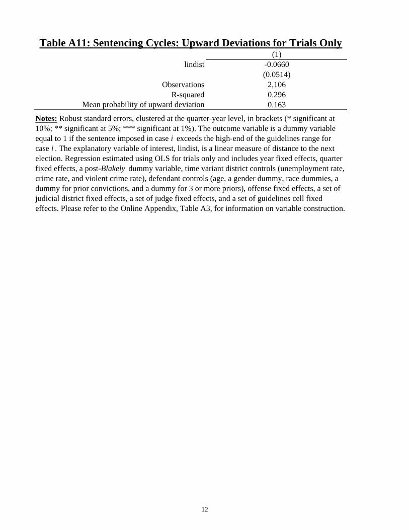
(1)lindist -0.0660

(0.0514)Observations 2,106

R-squared 0.296Mean probability of upward deviation 0.163

Table A11: Sentencing Cycles: Upward Deviations for Trials Only

Notes: Robust standard errors, clustered at the quarter-year level, in brackets (* significant at 10%; ** significant at 5%; *** significant at 1%). The outcome variable is a dummy variable equal to 1 if the sentence imposed in case i exceeds the high-end of the guidelines range for case i . The explanatory variable of interest, lindist, is a linear measure of distance to the next election. Regression estimated using OLS for trials only and includes year fixed effects, quarter fixed effects, a post-Blakely dummy variable, time variant district controls (unemployment rate, crime rate, and violent crime rate), defendant controls (age, a gender dummy, race dummies, a dummy for prior convictions, and a dummy for 3 or more priors), offense fixed effects, a set of judicial district fixed effects, a set of judge fixed effects, and a set of guidelines cell fixed effects. Please refer to the Online Appendix, Table A3, for information on variable construction.

12

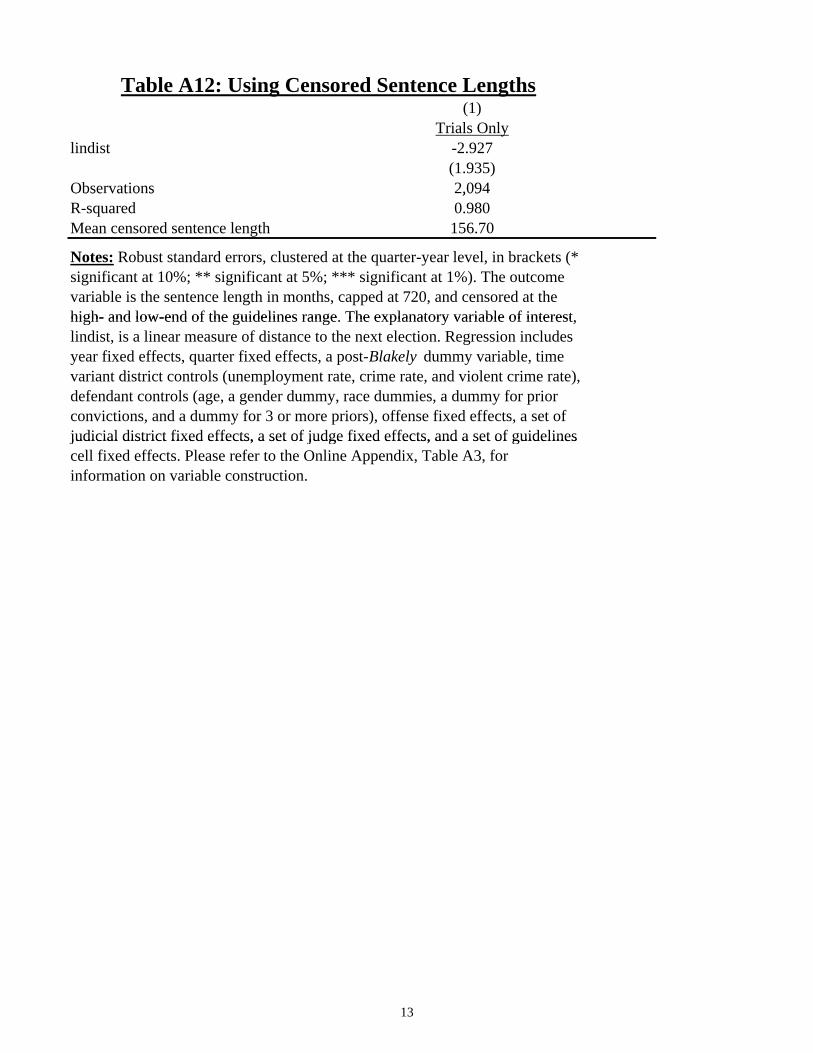
(1)Trials Only

lindist -2.927(1.935)

Observations 2,094

Table A12: Using Censored Sentence Lengths

Obse vat o s ,09R-squared 0.980Mean censored sentence length 156.70

Notes: Robust standard errors, clustered at the quarter-year level, in brackets (* significant at 10%; ** significant at 5%; *** significant at 1%). The outcome variable is the sentence length in months, capped at 720, and censored at the high- and low-end of the guidelines range The explanatory variable of interesthigh- and low-end of the guidelines range. The explanatory variable of interest, lindist, is a linear measure of distance to the next election. Regression includes year fixed effects, quarter fixed effects, a post-Blakely dummy variable, time variant district controls (unemployment rate, crime rate, and violent crime rate), defendant controls (age, a gender dummy, race dummies, a dummy for prior convictions, and a dummy for 3 or more priors), offense fixed effects, a set of judicial district fixed effects, a set of judge fixed effects, and a set of guidelines judicial district fixed effects, a set of judge fixed effects, and a set of guidelines cell fixed effects. Please refer to the Online Appendix, Table A3, for information on variable construction.

13

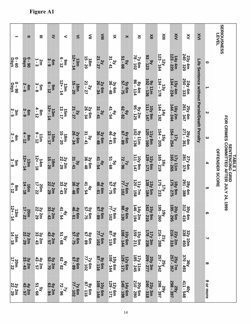
TABLE 1

SENTEN

CIN

G G

RID

FOR

CR

IMES C

OM

MITTED

AFTER JU

LY 24, 1999SER

IOU

SNESS

LEVELO

FFEND

ER SC

OR

E

01

23

45

67

89 or m

ore

XVI Life Sentence w

ithout Parole/Death Penalty

XV23y 4m

240 - 32024y 4m

250 – 33325y 4m

261 - 34726y 4m

271 – 36127y 4m

281 - 37428y 4m

291 - 38830y 4m

312 - 41632y 10m338 - 450

36y370 - 493

40y411 - 548

XIV14y 4m

123 - 22015y 4m

134 – 23416y 2m

144 - 24417y

154 – 25417y 11m165 - 265

18y 9m175 - 275

20y 5m195 - 295

22y 2m216 - 316

25y 7m257 - 357

29y298 - 397

XIII12y

123 - 16413y

134 – 17814y

144 - 19215y

154 – 20516y

165 - 21917y

175 - 23319y

195 - 26021y

216 - 28825y

257 - 34229y

298 - 397

XII9y

93 - 1239y 11m

102 – 13610y 9m

111 - 14711y 8m

120 – 16012y 6m

129 - 17113y 5m

138 - 18415y 9m

162 - 21617y 3m

178 - 23620y 3m

209 - 27723y 3m

240 - 318

XI7y 6m

78 - 1028y 4m

86 – 1149y 2m

95 - 1259y 11m

102 – 13610y 9m

111 - 14711y 7m

120 - 15814y 2m

146 - 19415y 5m

159 - 21117y 11m185 - 245

20y 5m210 - 280

X5y

51 - 685y 6m57 – 75

6y62 - 82

6y 6m67 – 89

7y72 - 96

7y 6m77 - 102

9y 6m98 - 130

10y 6m108 - 144

12y 6m129 - 171

14y 6m149 - 198

IX3y

31 - 413y 6m36 – 48

4y41 - 54

4y 6m46 – 61

5y51 - 68

5y 6m57 - 75

7y 6m77 - 102

8y 6m87 - 116

10y 6m108 - 144

12y 6m129 - 171

VIII2y

21 - 272y 6m26 – 34

3y31 - 41

3y 6m36 – 48

4y41 - 54

4y 6m46 - 61

6y 6m67 - 89

7y 6m77 - 102

8y 6m87 - 116

10y 6m108 - 144

VII18m

15 - 202y

21 – 272y 6m26 - 34

3y31 – 41

3y 6m36 - 48

4y41 - 54

5y 6m57 - 75

6y 6m67 - 89

7y 6m77 - 102

8y 6m87 - 116

VI13m

12+ - 1418m

15 – 202y

21 - 272y 6m26 – 34

3y31 - 41

3y 6m36 - 48

4y 6m46 - 61

5y 6m57 - 75

6y 6m67 - 89

7y 6m77 - 102

V9m

6 - 1213m

12+ - 1415m

13 - 1718m

15 – 202y 2m22 - 29

3y 2m33 - 43

4y41 - 54

5y51 - 68

6y62 - 82

7y72 - 96

IV6m3 - 9

9m6 – 12

13m12+ - 14

15m13 – 17

18m15 - 20

2y 2m22 - 29

3y 2m33 - 43

4y 2m43 - 57

5y 2m53 - 70

6y 2m63 - 84

III2m1 - 3

5m3 – 8

8m4 - 12

11m9 – 12

14m12+ - 16

20m17 - 22

2y 2m22 - 29

3y 2m33 - 43

4y 2m43 - 57

5y51 - 68

II0 - 90D

ays4m

2 – 66m3 - 9

8m4 – 12

13m12+ - 14

16m14 - 18

20m17 - 22

2y 2m22 - 29

3y 2m33 - 43

4y 2m43 - 57

I0 - 60D

ays0 – 90D

ays3m2 - 5

4m2 – 6

5m3 - 8

8m4 - 12

13m12+ - 14

16m14 - 18

20m17 - 22

2y 2m22 - 29

Figure A1

14

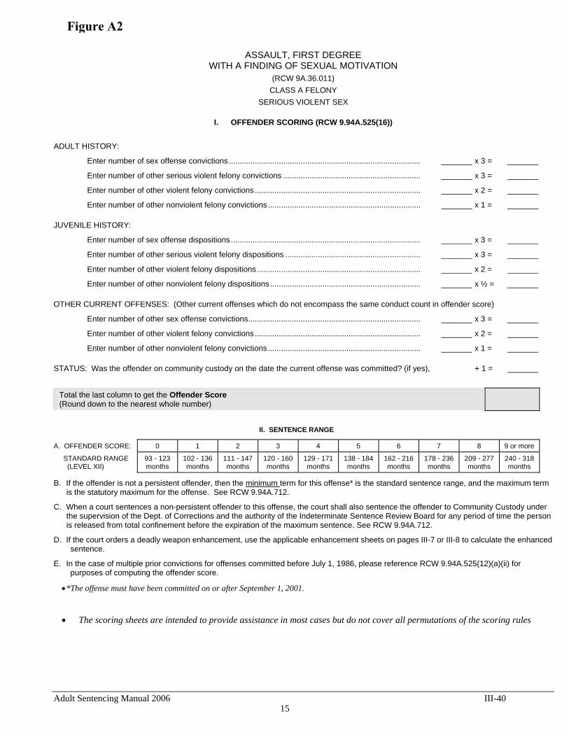
Adult Sentencing Manual 2006 III-40

ASSAULT, FIRST DEGREE WITH A FINDING OF SEXUAL MOTIVATION

(RCW 9A.36.011) CLASS A FELONY

SERIOUS VIOLENT SEX

I. OFFENDER SCORING (RCW 9.94A.525(16)) ADULT HISTORY:

Enter number of sex offense convictions........................................................................................ _______ x 3 = _______

Enter number of other serious violent felony convictions ............................................................... _______ x 3 = _______

Enter number of other violent felony convictions ............................................................................ _______ x 2 = _______

Enter number of other nonviolent felony convictions...................................................................... _______ x 1 = _______

JUVENILE HISTORY:

Enter number of sex offense dispositions....................................................................................... _______ x 3 = _______

Enter number of other serious violent felony dispositions .............................................................. _______ x 3 = _______

Enter number of other violent felony dispositions ........................................................................... _______ x 2 = _______

Enter number of other nonviolent felony dispositions..................................................................... _______ x ½ = _______

OTHER CURRENT OFFENSES: (Other current offenses which do not encompass the same conduct count in offender score)

Enter number of other sex offense convictions............................................................................... _______ x 3 = _______

Enter number of other violent felony convictions ............................................................................ _______ x 2 = _______

Enter number of other nonviolent felony convictions...................................................................... _______ x 1 = _______

STATUS: Was the offender on community custody on the date the current offense was committed? (if yes), + 1 = _______

Total the last column to get the Offender Score (Round down to the nearest whole number)

II. SENTENCE RANGE

A. OFFENDER SCORE: 0 1 2 3 4 5 6 7 8 9 or more

STANDARD RANGE (LEVEL XII)

93 - 123 months

102 - 136 months

111 - 147months

120 - 160months

129 - 171months

138 - 184months

162 - 216 months

178 - 236 months

209 - 277months

240 - 318months

B. If the offender is not a persistent offender, then the minimum term for this offense* is the standard sentence range, and the maximum term is the statutory maximum for the offense. See RCW 9.94A.712.

C. When a court sentences a non-persistent offender to this offense, the court shall also sentence the offender to Community Custody under the supervision of the Dept. of Corrections and the authority of the Indeterminate Sentence Review Board for any period of time the person is released from total confinement before the expiration of the maximum sentence. See RCW 9.94A.712.

D. If the court orders a deadly weapon enhancement, use the applicable enhancement sheets on pages III-7 or III-8 to calculate the enhanced sentence.

E. In the case of multiple prior convictions for offenses committed before July 1, 1986, please reference RCW 9.94A.525(12)(a)(ii) for purposes of computing the offender score.

• *The offense must have been committed on or after September 1, 2001.

• The scoring sheets are intended to provide assistance in most cases but do not cover all permutations of the scoring rules

Figure A2

15

Adult Sentencing Manual 2006 III-7

GENERAL DEADLY WEAPON ENHANCEMENT - FORM A Firearm or Other Deadly Weapon Enhancements*1

For offenses committed after July 23, 1995 Use of this form: Only for offenses committed after July 23, 1995 that have a firearm or other deadly weapon finding. CLASS A FELONY DEADLY WEAPON ENHANCEMENTS: First Deadly Weapon/Firearm Offense**: Subsequent*** Deadly Weapon/Firearm Offense: Firearm 5 years Firearm 10 years Other Deadly Weapon 2 years Other Deadly Weapon 4 years CLASS B FELONY DEADLY WEAPON ENHANCEMENTS: First Deadly Weapon/Firearm Offense**: Subsequent*** Deadly Weapon/Firearm Offense: Firearm 3 years Firearm 6 years Other Deadly Weapon 1 year Other Deadly Weapon 2 years CLASS C FELONY DEADLY WEAPON ENHANCEMENTS: First Deadly Weapon/Firearm Offense**: Subsequent*** Deadly Weapon/Firearm Offense: Firearm 18 months Firearm 3 years Other Deadly Weapon 6 months Other Deadly Weapon 1 year * Excluded offenses: Possession of a Machine Gun, Possessing a Stolen Firearm, Drive-by Shooting, Theft of a Firearm, Unlawful

Possession of a Firearm 1 and 2, Use of a Machine Gun in a felony, or any offense committed on or before July 23, 1995 with a deadly weapon finding.

** This enhancement is limited to offenses committed after July 23, 1995. *** To be sentenced as a subsequent deadly weapon finding, the offense in history with a deadly weapon finding must also have been

committed after July 23, 1995.

STANDARD RANGE CALCULATION CURRENT OFFENSE BEING SCORED

SERIOUSNESSLEVEL

OFFENDERSCORE

BASE STANDARD SENTENCE RANGE

TO

LOW HIGH

DEADLY WEAPON ENHANCEMENT

NOTE: The "base standard sentence range" is the appropriate standard

sentence without the deadly weapon enhancement.

STANDARD RANGE

TO

LOW HIGH

1For anticipatory offenses with a deadly weapon finding, add the enhancement after reducing the standard sentence range by 25%.

Figure A3

16

Statement on Plea of Guilty (Non-Sex Offense) (STTDFG) - Page 2 of 9 CrR 4.2(g) (8/2010)

(d) The right at trial to testify and to have witnesses testify for me. These witnesses can be made to appear at no expense to me;

(e) The right to be presumed innocent unless the State proves the charge beyond a reasonable doubt or I enter a plea of guilty;

(f) The right to appeal a finding of guilt after a trial.

6. In Considering the Consequences of my Guilty Plea, I Understand That:

(a) Each crime with which I am charged carries a maximum sentence, a fine, and a Standard Sentence Range as follows:

COUNT NO. OFFENDER

SCORE STANDARD RANGE ACTUAL CONFINEMENT (not including enhancements)

PLUS Enhancements*

COMMUNITY CUSTODY

MAXIMUM TERM AND FINE

1

2

3

* Each sentencing enhancement will run consecutively to all other parts of my entire sentence, including other enhancements and other counts. The enhancement codes are: (F) Firearm, (D) Other deadly weapon, (V) VUCSA in protected zone, (VH) Veh. Hom, see RCW 46.61.520, (JP) Juvenile present, (CSG) Criminal street gang involving minor, (AE) Endangerment while attempting to elude.

(b) The standard sentence range is based on the crime charged and my criminal history.

Criminal history includes prior convictions and juvenile adjudications or convictions, whether in this state, in federal court, or elsewhere.

(c) The prosecuting attorney's statement of my criminal history is attached to this agreement.

Unless I have attached a different statement, I agree that the prosecuting attorney's statement is correct and complete. If I have attached my own statement, I assert that it is correct and complete. If I am convicted of any additional crimes between now and the time I am sentenced, I am obligated to tell the sentencing judge about those convictions.

(d) If I am convicted of any new crimes before sentencing, or if any additional criminal history

is discovered, both the standard sentence range and the prosecuting attorney's recommendation may increase. Even so, my plea of guilty to this charge is binding on me. I cannot change my mind if additional criminal history is discovered even though the standard sentencing range and the prosecuting attorney's recommendation increase or a mandatory sentence of life imprisonment without the possibility of parole is required by law.

(e) In addition to sentencing me to confinement, the judge will order me to pay $500.00 as a

victim's compensation fund assessment. If this crime resulted in injury to any person or damage to or loss of property, the judge will order me to make restitution, unless extraordinary circumstances exist which make restitution inappropriate. The amount of restitution may be up to double my gain or double the victim’s loss. The judge may also order that I pay a fine, court costs, attorney fees and the costs of incarceration.

Figure A4

17