NBER WORKING PAPER SERIES

CREDIT SUPPLY AND HOUSE PRICES:EVIDENCE FROM MORTGAGE MARKET SEGMENTATION

Manuel AdelinoAntoinette SchoarFelipe Severino

Working Paper 17832http://www.nber.org/papers/w17832

NATIONAL BUREAU OF ECONOMIC RESEARCH1050 Massachusetts Avenue

Cambridge, MA 02138February 2012

We thank Viral Acharya, Chris Foote, Gustavo Manso, Atif Mian, Sendhil Mullainathan, Chris Mayer,David Scharfstein, Todd Sinai, Mathew Slaughter, Jeremy Stein, Bill Wheaton, and seminar participantsat the 2012 AEA Conference, CFS-EIEF Conference on Household Finance, Columbia Business School,Dartmouth College, Duke University, Federal Reserve Bank of Boston, Federal Reserve Bank of Philadelphia,Federal Reserve Board, McGill University, MIT Finance Lunch, NBER Asset Pricing and HouseholdFinance meetings, Princeton University, University of California at Berkeley, Weimer School May2012 Meetings, Western Finance Association 2012 Meetings, and Yale School of Management forthoughtful comments. We also thank Andrew Cramond from Dataquick for help with the data. Theviews expressed herein are those of the authors and do not necessarily reflect the views of the NationalBureau of Economic Research.

NBER working papers are circulated for discussion and comment purposes. They have not been peer-reviewed or been subject to the review by the NBER Board of Directors that accompanies officialNBER publications.

© 2012 by Manuel Adelino, Antoinette Schoar, and Felipe Severino. All rights reserved. Short sectionsof text, not to exceed two paragraphs, may be quoted without explicit permission provided that fullcredit, including © notice, is given to the source.

Credit Supply and House Prices: Evidence from Mortgage Market SegmentationManuel Adelino, Antoinette Schoar, and Felipe SeverinoNBER Working Paper No. 17832February 2012, Revised March 2013JEL No. D12,G10,R20

ABSTRACT

We show that easier access to credit significantly increases house prices by using exogenous changesin the conforming loan limit as an instrument for lower cost of financing. Houses that become eligiblefor financing with a conforming loan show an increase in house value of 1.16 dollars per square foot(for an average price per square foot of 220 dollars) and higher overall house prices controlling fora rich set of house characteristics. However, these estimated coefficients are consistent with a localelasticity of house prices to interest rates that is lower than some previous studies proposed (below10). In addition, loan to value ratios around the conforming loan limit deviate significantly from thecommon 80 percent norm, which confirms that it is an important factor in the financing choices ofhome buyers. In line with our interpretation, the results are stronger in the first half of our sample (1998-2001)when the conforming loan limit was more important, given that other forms of financing were lesscommon and substantially more expensive. Results are also stronger in zip codes where personal incomegrowth is low or declining, and in regions with lower elasticity of housing supply.

Manuel AdelinoDuke UniversityFuqua School of Business100 Fuqua DriveDurham, NC 27708-0120 manuel.adelino@gmail.com

Antoinette SchoarMIT Sloan School of Management100 Main Street, E62-638Cambridge, MA 02142and NBERaschoar@mit.edu

Felipe SeverinoMIT Sloan School of Management100 Main Street, E62-678Cambridge, MA 02142fseverin@mit.edu

An online appendix is available at:http://www.nber.org/data-appendix/w17832

1 Introduction

One of the central debates in finance is about the role of credit on the level of asset prices

and the creation of bubbles (Kiyotaki and Moore, 1997; Allen and Gale, 1998; Bernanke

and Gertler, 2001; Kindleberger, Aliber, Solow, 2005; Mian and Sufi, 2009; Brunnermeier,

Eisenbach and Sannikov, 2012). A salient recent example is the US housing market: many

observers of the crisis have proposed that easy access to credit, and the reduced cost of

credit, were the central factors fueling the increase in housing prices as well as the subse-

quent reversal in house price growth when credit dried up (Favilukis, Ludvigson, and Van

Nieuwerburgh, 2010; Hubbard and Mayer, 2008; Khandani, Lo, and Merton, 2009; Pavlov

and Wachter, 2010; Mayer, 2011). Proponents on the other side of the debate argue that

cheap credit alone cannot explain the house price boom and bust, and that other forces are

likely to have been at play (Glaeser, Gottlieb, and Gyourko, 2010).

The key difficulty in measuring the effect of credit on the price of housing is establishing

the direction of causality between credit conditions and house price growth: On the one

hand, easier and cheaper access to credit might reduce borrower financing constraints and

increase total demand for housing, which in turn would lead to higher prices. On the other

hand, however, credit conditions might be responding to expectations of stronger housing

demand and, as a consequence, higher house prices. In this latter scenario, cheaper credit

is not the driver of house price increases, but a byproduct of increased demand for housing,

since housing as collateral becomes more valuable. As we see in the existing literature, it

has been very difficult to separate these two effects.1

In this paper, we use annual changes in the conforming loan limit (CLL) as an instrument

for exogenous variation in the cost of credit, and in the availability of credit itself. The

CLL determines the maximum size of a mortgage that can be purchased or securitized by

Fannie Mae or Freddie Mac. This implicit (and since 2008, explicit) government support

for loans below the conforming loan limit provides easier access to credit for a wide range of

borrowers and reduces the cost of credit relative to jumbo loans. The difference in interest

rates between conforming loans and jumbo loans (those that are above the conforming limit)

is estimated to be up to 24 basis points in the 90’s and 2000’s (McKenzie, 2002; Ambrose,

LaCour-Little, and Sanders, 2004; Sherlund, 2008; Kaufman, 2012). Loutskina and Strahan

(2009, 2011) show that lenders screen borrowers for jumbo loans more intensely than they do

those that apply for conforming loans, which implies that mortgages below the conforming

loan limit are both cheaper and easier to obtain than above this limit.

1A recent paper by Favara and Imbs (2011) uses branching deregulation in the 1990s to identify the causallink between credit supply and house prices and finds that states where there is deregulation subsequentlyexperience larger house price increases.

2

The key idea of our identification strategy is that changes in the conforming loan limit

(CLL) from one year to the next are exogenous not only to individual transactions, but also

to the conditions of local housing markets or the local economy, since this change is based

on the countrywide average appreciation in house prices. Our empirical approach involves

comparing transactions with a price that can be financed more easily using a conforming

loan, and houses that are more expensive and for which buyers need to obtain larger loans

to maintain the same loan-to-value ratio. We track houses in this price range in the year

that the limit is in effect as well as the subsequent year, once the limit is raised and all

houses in the sample become eligible for conforming loans. This setup enables us to cleanly

identify the effect of the cost and access to credit based on the exogenous variation of the

CLL and control for any overall trends in house prices.

The threshold that we use to define houses that are “easy” to finance with a conforming

loan in a given year is the conforming loan limit divided by 0.8.2 By construction, buyers

of houses with a price below this threshold can get a conforming loan that makes up 80

percent of the price of the house, whereas, if the price of the house is above 125 percent of

the CLL, it can no longer be financed at 80 percent with a conforming loan.3 Above this

price threshold, borrowers either finance their home with an 80 percent first mortgage using

a jumbo loan (i.e. a loan above the CLL) at a higher interest rate, or, if they want to take

advantage of the lower interest rate below the CLL, they have to use savings or alternative

forms of financing to make a larger down payment.

The intuition behind this estimation strategy is that transactions that fall just above

the threshold are harder to finance, and thus, their prices have been bid up less relative to

the underlying fundamentals of the house. An increase in the conforming loan limit should

affect this part of the house price distribution more strongly since it allows borrowers who

previously were not able to get attractive financing to enter this segment of the market.

Importantly, our sample includes all transactions in this price range independent of the

financing choice of each borrower. This excludes any bias from our estimates that might

come from the endogenous choice of financing of a specific transaction, e.g. richer people

who can afford to put more money down might also purchase houses that are more expensive

based on (unobservable) quality dimensions.

We first confirm that the conforming loan limit has a significant impact on borrowers’

2Kaufman (2012) uses this threshold for appraisal values to study the effect of the conforming status ofa loan on its cost and contract structure.

380 percent loan to value ratios (LTV) are widely used in the industry as an important threshold forfirst lien mortgages. Loans with an LTV ratio below 80 are associated with more attractive terms andconforming loans above 80 percent require private mortgage insurance in order to qualify for purchase byFannie Mae or Freddie Mac (Green and Wachter, 2005).

3

choice of financing. The data shows that the norm in the mortgage market during this period

was to borrow at an LTV of exactly 0.8 (on average 60 percent of transactions are at an

LTV of 0.8). However, for houses that transact just above 125 percent of the CLL, a much

larger fraction of purchases are at an LTV below 0.8, since many borrowers choose to take

out a mortgage exactly at the conforming loan limit. This produces a large discontinuity

in the number of loans that are made at exactly the conforming loan limit, suggesting that

the CLL is an important determinant of mortgage finance. Borrowers that buy houses

with a price above the threshold of 125 percent of the CLL may choose a conforming loan

either because they are excluded from the jumbo loan market altogether, or because the

combination of a conforming loan and additional financing is a cheaper option. Whatever

the reason, these borrowers are de facto constrained in their choice of financing relative to

borrowers who buy houses at a price below 125 percent of the CLL.

In our main analysis, we test the impact of easier access to credit on house prices

instrumented via the change in the conforming loan limit. We run differences-in-differences

regressions in which we compare transactions just above and just below the threshold of 125

percent of the CLL in the year that the limit is in effect, and in the subsequent year when

all of the transactions can obtain an 80 percent conforming loan.4 We use three different

dependent variables to capture the value of a property: (1) the value per square foot; (2)

the residuals of log of house prices from a hedonic regression using a large set of controls

for the underlying characteristics of the house, and (3) the residuals of the value per square

foot from similar hedonic regressions. 5

We show that exogenous changes in the availability of credit due to changes in the CLL

have a significant effect on the pricing of houses that can be financed more easily using

a conforming loan. Specifically, we find that transactions in the “constrained” group of

borrowers, i.e. those with transaction values just above 125 percent of the CLL, are made

at lower values per square foot than those for the unconstrained group. We see a 1.16 dollar

discount per square foot for a mean value per square foot of 220 dollars and mean size of

1935 square feet. This difference is still significant but reduced to 0.65 dollars per square

4This is the case for all years between 1998 and 2005. For example, the CLL in 1999 is USD 240, 000,which gives a threshold of USD 240, 000/0.8 = 300, 000 for this year. This means that in the regression for1999, we include houses priced at between 290, 000 and 310, 000 in the years of 1999 (the year the CLL isin effect) and 2000. The CLL in the year 2000 was raised to 252, 700, so the new threshold for that year is315, 875. Clearly, all the houses we included in the analysis for 1999 can be financed at 80 percent with aconforming loan in the year 2000.

5We run the hedonic regressions by year and by metropolitan statistical area (of which we have 10)and we use the set of controls available from deeds registries data, which includes common variables suchas number of rooms and number of bedrooms, but also detail on the type of heating, architectural type,building type, among many others (we discuss these controls in more detail in Section 3.2).

4

foot after we control for house characteristics, suggesting that part of the effect we find can

be accounted for by differences in the observable quality of houses above and below the

threshold. The effect is smaller (and often insignificant) in the second half of our sample

(2002-2005), which is the period when jumbo loans became cheaper and easier to obtain

(partly due to the increased ease with which they could be securitized) and also when second

lien mortgages became widely available (see Figure 1 in the Online Appendix). Both these

effects go in the direction of making the CLL less important in the latter part of the sample,

since borrowers above and below the threshold were getting similar access to finance.

Given our estimate for the change in house prices due to changes in credit conditions, we

can compute the semi-elasticity of prices to differences in interest rates in the region close

to the threshold. As our measure of the cost differential faced by buyers above and below

the threshold, we use the differences in interest rates estimated in the prior literature of

10 to 24 basis points between conforming and jumbo loans. We obtain elasticity estimates

that range from a low end of 1.2 to an upper range of 9.1 depending on the period and the

exact estimate for the interest rate differential between jumbo and conforming loans that we

use for our calculations. Therefore, when we use exogenous variations in the ease of credit

conditions, we find elasticity estimates that are at the lower end of what has been previously

found in the literature. This suggests that it is of first order importance to control for the

endogenous decrease in the cost of capital in times when house price appreciation is high.

One basic assumption underlying our analysis is that the CLL provides a significant

improvement in the cost of funding and in the access to finance for people buying houses

at a price just around the threshold. We expect this effect to be stronger when buyers face

other types of constraints at the same time, namely in terms of their income. To test this

intuition, we interact the changes in the CLL with the economic condition of the average

household in a neighborhood. We find that the effect of credit supply on value per square

foot is much stronger in zip codes and years that are below the 10th percentile of the income

growth for each individual regression. The point estimate for these areas shows that value

per square foot is 2.50 dollars higher in the year that a house becomes eligible to be financed

with a conforming loan. This is more than double the size of the average effect that we

found in the overall sample.

We also test whether our instrument has an impact on the number of transactions

we observe above the threshold. There is no visible bunching of transactions around the

threshold of CLL divided by 0.8, suggesting that the supply of housing does not react

strongly to the CLL. In our empirical tests we find no significant effect of our instrument

on the quantity of houses transacted during the first half of the sample. We do see fewer

transactions above the threshold in the period 2002-2005, which may help explain the weaker

5

response in prices that we find in the later period.

Our estimation strategy allows us to estimate the causal effect of changes in credit

availability on the valuation of houses. Since house price levels differ across the various

states of the United States, the change in the CLL affects different parts of the housing

stock across areas depending on the price level of the area. This allows us to control for

the possibility that there are differential growth rates within the distribution of house types

across the country. For example, one concern would be that middle class families might

be the ones buying a certain type of house and, at the same time, have a different income

growth from other parts of the economy. Our instrument allows us to rule this out, because

the same “type” of house will have different prices depending on the part of the country in

which it is located. However, we do not observe the exact mechanism through which credit

conditions feed through to house prices. There are at least two alternative ways that credit

could affect prices: First, better access to credit increases demand for houses since more

people can now bid on properties, and as a result, we see an increase in the price of the

transactions. A second and alternative channel would be that borrowers who have easier

access to finance bargain less hard for a reduction in property prices relative to borrowers

who struggle to find financing. Importantly, in either of these channels a change in access

to finance is driving the change in borrower behavior and consequently house prices.

We can rule out an alternative hypothesis related to a selection effect driving our results,

whereby buyers of houses “above the threshold” in the year that the conforming loan limit is

in effect are different along some unobservable characteristics from the other buyers. Several

features of our analysis make selection an unlikely explanation of the results. First, for a

selection hypothesis to be a true alternative to our explanation of the results, it would have

to involve arguments other than access to credit to explain why buyers were different above

and below the threshold. Second, these “special” buyers would both have to be better able

to deal with the reduced access to credit (potentially because they are wealthier or have

higher income) and bargain harder for houses. It is unclear why wealthier borrowers should

pay less for a similar house than poorer borrowers. If wealthier people bought higher quality

houses and we did not observe these differences, these unobservable characteristics would

create bias in the opposite direction. Third, our identification strategy would require that

the selection effect change each year parallel to the change in the size of the conforming

loan limit, which is very unlikely. Finally, to help further rule out this selection hypothesis,

we run our main regressions excluding borrowers that choose LTVs below 80 percent in

the year that the CLL is in effect. If selection was the explanation of the results, these

transactions should be by “wealthy” borrowers driving the results. We find that the results

do not change materially when we exclude this subset of transactions.

6

The rest of the paper is structured as follows: Section 2 discusses related literature and

the user cost model. Section 3 describes our data and the identification strategy. In Section

4, we lay out the regressions results and robustness checks of our main analysis. Section 5

discusses the findings and concludes.

2 The User Cost Model

In this paper, we are interested in estimating the impact of changes in credit conditions

on the price of housing. The existing literature has focused on different versions of the

user-cost model of Poterba (1984) to draw conclusions about the role of interest rates and

other costs of owning for house prices. In this model, agents are indifferent between owning

and renting if the housing market is in equilibrium, where the mortgage interest rate is the

main determinant of the cost of owning. Below, we show that different assumptions yield

very different conclusions about the role of interest rates in driving the cost of housing and

highlight why our estimate of the impact of the cost of credit on prices is an important

contribution to this debate. We follow the notation in Glaeser, Gottlieb, and Gyourko

(2010) to describe the basic elements of the user cost model. Renting a property involves

paying rent equal to Rt in each period. Owning a property, on the other hand, includes

making a down-payment θ that is a proportion of the price of the house Pt and obtaining a

mortgage that is rolled over each period, such that principal is never paid down completely.

The borrower then pays interest on the mortgage at a rate rt that is deflated by the relevant

tax rate φ, as well as property taxes and maintenance costs equal to τ that both grow at

a rate g. The model assumes that individuals have a private discount factor of ρt. If we

assume that market interest rates and private discount rates are constant and equal to each

other, we can write the indifference condition for users as:

Rt

Pt

= (1− φ)r − g + τ (1)

This is shown in Glaeser et al (2010) and is similar to what is presented in Hubbard and

Mayer (2008) as well as a simplified version of the user cost in Himmelberg, Mayer, and Sinai

(2005). If the assumptions of this model hold, changes in the user cost (the right-hand side

of the equation) should lead to changes in the price to rent ratio according to this formula.

For example, if the user cost is 5 percent, then the price of a house should be about 20 times

its market rent. In such a world, a drop of 1 percentage point in mortgage rates would lead

to a decline of (1−τ) in the user cost, or 0.75 if we assume a marginal tax rate of 25 percent.

The price to rent ratio would then be 23.5, an increase in the price of 17.5 percent. This

7

is the magnitude of the elasticities proposed in Himmelberg et al (2005), and in Hubbard

and Mayer (2008). Glaeser, Gottlieb, and Gyourko (2010) dispute some of the simplifying

assumptions in the model above, and show that a more realistic model can produce much

lower elasticities of prices to interest rates. In particular, if private discount rates are not

the same as market rates, then changes in interest rates wont change the way users discount

future expected house price appreciation. This change alone can reduce the elasticity to

just 8, instead of the initial 17.5. Glaeser et al (2010) propose other mechanisms through

which the elasticity could be substantially reduced, namely mean reverting interest rates,

which means borrowers anticipate having to sell a home at a time when rates are higher,

or the possibility of prepaying a mortgage, which again lowers the predicted elasticity. Our

econometric approach allows us to more carefully identify the magnitude of the change in

house prices due to changes in the average cost of financing, since we look at exogenous

movements in the cost of capital for home buyers. Our empirical results provide estimates

for the numerator of the elasticity calculation. In Section 4.4, we discuss the range of

elasticities that are consistent with our results.

3 Data and Methodology

The dataset we use in this paper contains all the ownership transfers of residential properties

available in deeds and assessors records for the cities that are covered by Dataquick. Our

dataset spans 11 years, from 1998 to 2008, and contains all transactions recorded on the

deeds registries for seventy-four counties in ten metropolitan statistical areas (MSAs) -

Boston, Chicago, DC, Denver, Las Vegas, Los Angeles, Miami, New York, San Diego, and

San Francisco. We limit our attention to transactions of single-family houses, which account

for the large majority (approximately 78 percent) of all observations.

Each observation in the data contains the date of the transaction, the amount for which

a house was sold, the size of the first mortgage, and an extensive set of variables about the

property itself. These characteristics include the property address, interior square footage,

lot size, number of bedrooms, number of bathrooms, total rooms, house age, type of house

(single-family house or condo), renovation status, and date of renovation. Additional, more

detailed characteristics, include the availability of a fireplace, parking, the architectural and

structural style of the building, the type of construction, exterior material, availability of

heating or cooling, heating and cooling mechanism, type of roof, view, attic, basement, and

garage. We describe the procedure for cleaning the raw data received from Dataquick in

the Online Appendix to the paper.

8

3.1 Summary Statistics

The sample that we use for this paper contains 3.9 million transactions of single-family

houses that are summarized in Tables 1 and 2. We can see in Panel A of Table 1 that

the average transaction value in our sample is 308,520 dollars with a standard deviation of

123,930 dollars. The average size of the houses in the cleaned dataset is 1,735 sqft, and the

houses have, on average, 3 bedrooms and 2 bathrooms. The average loan to value is 0.81

(including only the first mortgage for each transaction), and the median LTV is 80 percent.

The average value per square foot is 194 dollars with a standard deviation of 92 dollars per

square foot (first row of Panel B).

Table 1 also shows the summary statistics for the restricted sample we use in the regres-

sions in the final three columns. For the restricted sample6 , the average price for each house

is higher than in the whole dataset, the average value per square foot is 220 dollars with

a standard deviation of 93 dollars per square foot, given that this subsample includes only

houses that are close to the conforming loan limit. This is consistent with the fact that the

conforming loan limit was set to cover substantially more than 50 percent of the mortgages

made every year (Acharya, Richardson, Nieuwerburgh, White, 2011). These houses are

also, on average, larger and have more bedrooms and bathrooms than the whole Dataquick

sample.

Panel A of Table 2 shows marked differences in the summary statistics for each of the ten

MSAs included in our data. The table shows that San Francisco is the metropolitan area

with the highest valuation, with an average house price of 384 thousand dollars. Denver and

Las Vegas represent the areas with the lowest valuation, with an average of approximately

250 and 262 thousand dollars respectively. When we compare values per square foot, we

get a similar picture, namely San Francisco is the area with the highest valuation with an

average of 266 dollars per square foot, and Las Vegas is the area with the lowest valuation

with an average of 137 dollars per square foot.

Table 2 Panel B shows the evolution of prices through time. Here we see the increase

in house prices from an average of 240 thousand dollars in 1998 to a peak of 366 thousand

dollars in 2006, as well as the increase in the volume of transactions over the same period.

The increase in prices and volume is linked to an increase in volatility. The standard

deviation of the transactions increased from 102 thousand dollars in 1998 to 122 thousand

dollars in 2006. A similar pattern can be observed for the value per square foot measure,

where standard deviation is 51 dollars per square foot in 1998, and increases to 106 dollars

per square foot in 2006. Finally, the loan to value average (including only the first mortgage)

6In this case, transactions that are used as control for one year, and treatment in the following period, areduplicated to reflect the statistics of the regression sample, the augmented data set has 262,671 observations

9

is stable both across MSAs and through time at around 0.8.

3.2 Hedonic Regression

One of the advantages of using deeds registry data is the richness of the information provided

on the property characteristics, which allows us to account for price differences between

houses that can be attributed to observable features. Specifically, we will be able to assess

whether the price impact we observe due to the changes in the conforming loan limit can be

attributed to differences in the quality of the houses, or whether these differences are there

even after accounting for quality.

In order to distinguish between these two explanations, we estimate hedonic regressions

of value per square foot and log of house price on a number of house characteristics, and

estimate the residuals for each of these two left-hand side variables (which we denote by

LHSi). Specifically, we estimate the following regressions by MSA and by year:

LHSi = γ0 + ΓXi +monthi + zipcodei + εi

We use both the price of a transaction as well as the value per square foot as our

dependent variables. By estimating these regressions by year and by MSA, we allow the

coefficients on the characteristics to vary along these two dimensions. We also use monthly

indicator variables to account for seasonality in the housing market, as well as zip code

fixed effects. The set of controls Xi is a similar set of controls to that used in Campbell,

Giglio, and Pathak (2010) with some additional characteristics. The controls include square

footage, high and low square footage dummies, the size of the lot, number of bedrooms and

bathrooms, and a number of indicators for interior and exterior house characteristics (eg.

fireplace, style of the building, etc.). We describe which variables are included, as well as

the detail of the construction of each variable, in the Online Appendix to the paper.

The estimated R2 of each of these regressions (80 in total for each of the two left-hand side

variable–10 MSAs in 8 years) is between 40 and 60 percent for the price of the transaction,

and 50 to 70 percent when we use value per square foot as a dependent variable7.

Summary statistics for the residuals from the hedonic regressions for the whole sample

are shown in Panel B of Table 1. The average residuals are, by construction, zero. The

standard deviation of the errors is about 42 dollars per square foot, and 0.17 thousand

dollars for the log of the price of the house. The hedonic regressions are estimated on the

whole clean sample8, so when we restrict our attention to the regression sample, the average

7Unreported regressions.8Please see the Online Appendix for a detailed description of what is included in this subset of the data.

10

error no longer has to be zero. Indeed, for the regression sample, the average residual

from the hedonic regressions for the value per square foot is positive at 5.3 dollars, and the

average error for the log of transaction value of the house is 0.05 dollars (last three columns

of Panel B of Table 1). The standard deviation of the residuals for the regression subsample

is similar in magnitude to what we obtain for all the transactions.

3.3 Empirical Approach

3.3.1 Identification Strategy

To identify the effect of changes in credit conditions on house prices, we restrict our analysis

to two groups of buyers who all buy houses in a tight price range, but differ in the financing

available to them. The sample for our regressions is made up of houses that transact in

a band around 125 percent of each year’s conforming loan limit, as well as houses in the

subsequent year in the same price range. Specifically, we divide houses into two groups:

houses below the threshold of 125 percent of the year’s CLL (i.e. transactions that fall

between 125 percent of CLL and 125 percent of CLL minus USD 10,000) and houses above

that threshold that transact between 125 percent of CLL and 125 percent of CLL+10, 000.

By construction, in the year that the conforming loan limit is in effect, houses above the

threshold of 125 percent of the CLL cannot be financed at 80 percent using a conforming

loan, whereas the houses below the threshold can be financed. Thus, home buyers that

bid for houses priced above 125 percent of CLL cannot finance a full 80 percent of the

transaction with the cheaper and more easily available conforming loans. In the subsequent

year, the CLL is raised and both groups of transactions can be financed at 80 percent with

a conforming loan.9 Our sample includes all transactions in this price range, independent

of the mortgage choice made by each buyer. This way, our estimates are not biased by the

endogeneity of the choice of financing of each specific transaction.

The identification strategy is best understood through an example. Consider the year

1999: In that year, the conforming loan limit (CLL) for single-family houses was USD

240, 000. The corresponding threshold for house prices that we use for this year is 300, 000

(240, 000/0.8 or, equivalently, 1.25 ∗ 240, 000). In this year, the group of houses “above the

threshold” have prices between USD 300, 000 and USD (300, 000 + 10, 000) = 310, 000 and

houses “below the threshold” have a transaction price between USD (300, 000− 10, 000) =

290, 000 and USD 300, 000 (those that transact at exactly USD 300, 000 are included in

9While this was no longer true for the years after 2006, in all cases between 1998 and 2005, the limitincreases enough from year to year to make up 80 percent of the price of the transactions we have in thesample.

11

this second group). For the purposes of our main regressions, we track these two groups of

houses from 1999 to 2000, where 1999 is the year in which the CLL is in effect and 2000 is

the year in which all these transactions could be bought using a conforming loan at a full

80 percent LTV. In fact, the CLL changed in 2000 to USD 252, 700, so the threshold of 125

percent of CLL was now USD 315, 875 and even our “above the threshold” group for 1999

is now eligible to get an 80 percent LTV conforming loan.

One important assumption in our analysis is that borrowers in the group “above the

threshold” of 125 percent are constrained in their choice of financing. In order to stay at an

LTV of 0.8, they have to take a jumbo loan and these have been found to be more expensive

by between 10 and 24 basis points relative to conforming loans (McKenzie, 2002; Ambrose,

LaCour-Little, and Sanders, 2004; Sherlund, 2008; Kaufman, 2012). Alternatively, they can

also borrow up to the CLL and then cover the rest of the house price with savings or other

funding, which means having a first mortgage LTV of less than 80 percent. This additional

source of funding is likely substantially more expensive relative to the conforming mortgage

rate. For some borrowers, this may, in fact, be the only option, as they may be excluded

from the jumbo market altogether because of more careful screening of jumbo loans done

by originating banks (Loutskina and Strahan, 2009, 2011). Whether they choose a jumbo

loan or they make up the difference using other sources of financing, these borrowers have

a higher average cost of capital than the buyers below the threshold. Figure 1 shows the

frequency of transactions by price and choice of first mortgage (both in USD 10,000 bins).

The figure shows that the most frequent choice on the part of borrowers is to have an LTV

of exactly 80 percent (that is, the large mass along the diagonal of the figure). The main

exception to this rule occurs exactly at the conforming loan limit, where a significant mass

of borrowers chooses an LTV below 0.8 by sticking to a conforming loan (in 2000 the limit

was USD 252,700, and in 2004 it was 333,7000). In unreported analyses, we find that in the

year in which the CLL is in effect, about 45 percent of the houses below the threshold in

our sample are bought with an LTV of exactly 80 percent, whereas, for houses above this

boundary just 19 percent of borrowers pick 80 percent LTVs (which for these transactions

means using a jumbo loan). Additionally, on average 55 percent of the transactions just

above the threshold are financed using a conforming loan, which means having an LTV

lower than 80 percent. These borrowers end up with an LTV of 77-79.5 percent, which is

a very infrequent choice anywhere else in the distribution. Again, these borrowers might

have a lower LTV because they choose to stay below the CLL due to the cost of the loan,

or because they are excluded from the jumbo market altogether. Whatever the reason, this

group of borrowers is “constrained” in the set of options available for financing their house.

12

3.3.2 Empirical Specification

Our main regressions estimate the size of the effect of the constraint imposed by the con-

forming loan limit on the valuation of transactions made just above the threshold of 125

percent of the CLL. We run differences-in-differences regressions year-by-year with one in-

dicator variable for houses priced above the conforming loan limit divided by 0.8, another

indicator for the year in which the CLL is in effect, and an interaction of these two indicator

variables. We also include ZIP code fixed effects in all regressions, so our estimates do not

reflect differences between neighborhoods, but rather variation within zip codes.

The sample for each year-by-year regression includes houses within a USD 10,000 band

around the conforming loan limit in the year in which the limit is in force, as well as the

subsequent year. This implies that the “Above the Threshold” indicator variable takes

a value of 1 if the price at which a house transacts is greater than 125 percent of the

conforming loan limit of a certain year, and less than that amount plus 10,000 dollars. This

same variable is a 0 for transactions between 125 percent of the CLL and 125 percent of the

CLL minus 10,000 dollars. The “Year CLL” indicator variable is a 1 in the year in which

the CLL is in effect for each regression, and a 0 in the subsequent year. We use a tight

band around the threshold so that all transactions in the year after the limit is in effect are

eligible for an 80 percent LTV conforming loan. We thus have a group of transactions that

is “easy to finance and another one that is “hard to finance in the year that the limit is in

effect, but all transactions in the sample are “easy to finance once the limit is raised.

We run regressions of the following form:

V aluation measurei = β0+β11AboveThreshold+β21Y ear CLL+β31Above Threshold×Y ear CLL+γZIP+εi

We estimate this regression for each year between 1998 and 2005. We cannot include

2006 and 2007 in our estimates because the conforming loan limit did not change after

2006 in our data (house prices dropped and the administration left the limit unchanged).

After we obtain β1, β2, and β3 for all 8 years (1998-2005), we estimate Fama-MacBeth

averages (Fama and MacBeth, 1973) of these coefficients and obtain the standard errors of

this average by using the standard deviation of the estimated coefficients and dividing it by

the square root of the number of coefficients.

We should point out that our approach is not a regression discontinuity design, but

rather differences-in-differences for each pair of years. There are a couple of reasons for this:

First, the threshold that we use does not imply a sharp discontinuity in the ease of financing

a home. For a house just one dollar above the threshold, a homebuyer only has to come up

13

with one additional dollar of equity (and still obtain a conforming mortgage), which means

the total cost of financing the house is almost unchanged. As we move progressively away

from the threshold, transactions become harder to finance. For our differences-in-differences

estimator to be valid, all we need is that houses above the threshold are somewhat harder

to finance, though not necessarily discontinuously so.

The second reason for not using a regression discontinuity design is that in the year that

the limit is in effect, homebuyers choose to buy houses above or below the threshold, i.e.

the position with respect to the limit is not exogenous. On the contrary, our differences-in-

differences specification uses the exogenous change in the conforming loan limit to compare

a group of transactions that are above the limit in a year, but below in the next with a

group of transaction that are always below the limit, achieving a clean identification of the

effect of credit availability on house prices.

3.3.3 Differences in Financing Choices

As we pointed out above, the equivalent to a first stage in our empirical strategy is to show

that the changes in the conforming loan limit have a significant effect on the financing choices

of borrowers. In Figure 1 we can see the importance of both the 80 percent LTV rule, as

well as the conforming loan limit, in determining financing choices for the whole distribution

of transactions. In Figure 2 we focus on the groups of transactions that we include in the

regressions. The first panel tracks transactions up to USD 10,000 below 125 percent of the

conforming loan limit in each year, whereas the second panel includes transactions up to

USD 10,000 above the threshold. We show the total number of transactions (for all years

between 1998 and 2006) in each month during the year prior to the limit being in effect,

in the year that the limit is valid, and in the subsequent year. We also break down the

transactions by the choice of LTV - the transactions at the bottom of each panel have an

LTV below 75 percent, the second group includes transactions with an LTV between 75

percent and 79.5 percent, the third has transactions with LTV=80 percent, and the top

group has all the transactions with an LTV above 80.1 percent. The main message from

Figure 2 is that in the year that the CLL is in effect, the composition of financing choices

by borrowers differs very significantly, with the 80 percent group becoming very prominent

for the transactions below 125 percent of the CLL, whereas it is small for the transactions

above the threshold. At the same time, the borrowers who stick with a conforming loan and

buy houses above 125 percent of the CLL become an important fraction of all borrowers

(they have an LTV between 75 and 79.5 percent).10 In the year after the limit is in effect,

10The first picture for the group below 125 percent of the CLL also shows a noticeable fraction ofborrowers with an LTV between 75 and 79.5 percent in the year before the CLL is in effect. This is because

14

the choice of LTV across the two groups becomes indistinguishable.

In Table 3, we present the effect of the changes in the conforming loan limit on the

financing choices made by the borrowers included in the sample of our main regressions. In

this table, we are verifying what we see in the pictures, namely that borrowers on average

end up with lower LTVs when they buy houses above the threshold of 125 percent of CLL.

Results for the effect of the CLL on financing choices are shown in Table 3. We find that

LTVs are, on average, 0.3 to 0.7 percentage points lower for the group of transactions that

happen above the threshold of 125 percent of the CLL in the year that the limit is in effect.

This effect is statistically and economically significant given how little variation there is in

the modal choice of LTV of borrowers. The second panel on Table 3 shows that borrowers

also obtain, on average, smaller loans in the year that the limit is in effect and when the

price of the house is above the threshold. The difference in log loan amount is, on average,

0.0056 to 0.0088 dollars, and based upon the findings in our main results, we conjecture

that it is the fact that borrowers obtain smaller first mortgages that leads to the difference

of approximately 1.16 dollars per square foot (for an average value per square foot of 220

dollars).

3.3.4 Differences in the Number of Transactions

There are several reasons to expect quantities to change due to differential ease in access to

credit, including different levels of down-payment (Stein, 1995) or sellers waiting for buyers

to obtain better credit conditions (Genesove and Mayer, 1997). In fact, unless the supply

elasticity of houses is very low (or zero), we expect the price effect due to a change in the

demand for housing to be accompanied by a change in the number of transactions.

As discussed in Section 3.3.2, we do not use a regression discontinuity approach to

address the question of the change in the quantity of transactions. Figure 3 confirms that

this would produce no significant result. This figure shows the number of transactions

relative to the threshold in each year. The figure is centered at “0, i.e. the transactions

at exactly 125 percent of the CLL. The figure shows that there is no discontinuity in the

number of transactions above and below the threshold. We confirmed this result by splitting

the sample into old and new houses, different MSAs, and in the first half and second half

of each year (all unreported).

Given that a regression discontinuity would not be appropriate in our setting, we use

these transactions were not eligible for a conforming loan at an 80 percent LTV in the year before the newlimit was in effect and were, in general, just slightly above that threshold. This is thus a reflection of thesame phenomenon we see for the group above 125 percent of the CLL in the year that the new limit is inplace.

15

a setup similar to our main regressions to look for changes in the number of transactions

above and below the threshold. We consider the difference in the share of transactions in our

sample that fall above and below the threshold in the year that the limit is in effect and in

the subsequent year in a differences-in-differences setup. This test is equivalent to a T-test

for the mean of the variable “Above Threshold” that compares the average of this variable

in the year that the limit is in effect and in the subsequent year. If our instrument affects

the quantity of transactions, we should see an increase in the share of observations above the

threshold when the limit is raised, as access to credit become easier for those transactions.

We show in Table 4 that this test reveals no changes in the share of transactions above

and below the threshold for the first part of our sample (1998-2001), and that there is a

statistically significant effect for the second part of the sample. This effect means that the

share of transactions above the threshold is approximately 50 basis points lower in the year

that the conforming loan limit is in effect during the period 2002-2005. This shows that

the effect of cheaper credit provided by conforming loans is reflected only on house prices

in the first part of our sample, and that in the second part of the sample, it impacts both

quantities and prices, i.e. supply elasticity of houses seems to have been higher in the second

part of the sample. This, along with the reasons we give in Section 4.1 on the availability of

second liens and jumbo loans, may help explain why the effect we find on prices is smaller

relative to the earlier years (when the quantity response was not there).

4 Access to Credit and House Prices

4.1 Main Regression Results

We present the results for our canonical specification in Table 5. This table presents Fama-

MacBeth coefficients from year-by-year regressions, as described before in Section 3.3.2. The

coefficient of interest in Panel A of Table 5 is that on the interaction variable, and it shows

that houses above the threshold of CLL/0.8 transacted at a value per square foot that was

lower by about 1.16 dollars in the year that the CLL was in effect. The results are stronger

for the first half of the sample, where the point estimate is -1.55 dollars per square foot for

this set of transactions.

The other coefficients on the regressions for value per square foot are consistent with what

we know about house prices over this period. First, houses that are above the threshold of

125 percent of CLL (i.e. the more expensive houses in the regression sample) are associated

with a higher average value per square foot. In unreported analyses, we find that more

expensive houses are generally associated with a higher value per square foot (i.e. price

16

rises quicker than house size in the whole distribution of transactions), and here we find

that this is also the case for the regression sample. Also, the “Year CLL” dummy variable

is associated with a strong negative effect, reflecting the strong increase in house valuations

that we saw in this period in the US. Given that the year in which the CLL is in effect is

always the “pre” year in the regressions, we expect those transactions, on average, to be

associated with a lower value per square foot.

In Panels B and C we use the residuals from the regressions we described in Section 3.2

as the dependent variable to account for differences in quality between houses. The results

are qualitatively and quantitatively very similar to the ones we present in Panel A. In Panel

B we are using the residuals of a regression of log of house price on a set of characteristics,

and we find a point estimate of -0.0017 that translates to residual being lower by 620 dollars

for houses above the threshold of 125 percent of the CLL when the CLL binds, considering

an average transaction value of 371,340 dollars. This suggests that transactions that cannot

be financed at 80 percent with conforming loans are made at lower prices even after we

control for a rich set of house characteristics.

Similarly in Panel C of Table 5, we confirm that even when we use the value per square

foot as a dependent variable but control for house quality, the interaction term is significant

and economically large even though the point estimate of 0.65 dollars for houses above the

threshold is slightly lower than the results in Panel A where we do not adjust for house

quality. The difference between the point estimate of 1.16 dollars of Panel A and 0.65

dollars in this specification indicates that houses above the limit are of somewhat worse

quality than those below the limit in the year that the limit is in effect.

We also show that the estimated effect of the conforming loan limit on house prices is

stronger in the first half of the sample than in the second half. This result holds for all three

left-hand side variables. This is in line with our expectations, given that borrowers had

easier access to second lien loans after 2002 (we show the evolution of the use of second liens

in Figure 1 of the Online Appendix). Additionally, more borrowers use jumbo loans, which

may reflect a reduction of the cost differential of this type of loan relative to conforming

loans, and an increase in the ease of access to this type of loan, possibly driven by an

increased ease of securitization of these loans.

4.2 Credit Supply and Income

We now turn to how the effect of credit supply on house prices changes with the growth in

income in a zip code. To do this, we obtain data on zip code level average household income

17

each year from 2000 to 2007 from Melissa Data.11 We create a new variable that is a “1” if

a zip code has negative nominal average income growth from one year to the next, and “0”

otherwise. We then run similar regressions to what we did before (year-by-year), adding

an interaction between our previous variables and this new zip code level “Negative Income

Growth” variable. Looking at the coefficient on the triple interaction term (negative income

growth, the year that the CLL is in effect, and being above 125 percent of the CLL) allows

us to identify how the effect of credit supply differs in times of positive and negative income

growth. Our hypothesis is that the effect of credit supply is stronger in times of negative

income growth, as households in a certain zip code are more likely to be constrained and

there is likely to be less competition for housing, which increases the probability that a seller

sells to a constrained buyer.

We show the results for these regressions in Table 6. In the first column of Table 6 we

repeat our main regressions for the period 2001-2005 only, as this is the period for which we

were able to construct the income growth indicator variable. The results are consistent with

those in Table 5. In the second column of Table 6 we show Fama-MacBeth coefficients from

the regressions with the income growth interaction term. The triple interaction terms show

that the effect of credit supply on value per square foot is significantly stronger in zip codes

and years that are below the 10th percentile of income growth for the individual regression.

The point estimate shows that value per square foot is 1.55 dollars lower in the year that

the conforming loan limit is in effect for houses above 125 percent of the limit when income

growth is low in a zip code. We also find that the main effect from our regressions in Table

5 is quantitatively similar to before, implying that the simple inclusion of ZIP code level

income does not change any of our main results.

In the Online Appendix we plot the distribution of value per square foot for ZIP codes of

different income levels. Those pictures also suggest that the distribution of value per square

foot is affected by the conforming loan limit in ZIP codes in the lowest quartile of the income

distribution. In particular, the average value per square foot is monotonically increasing for

up to conforming loan limit threshold, and from this point onwards the distribution becomes

flat. This pattern is not visible for zip codes with higher median incomes.

4.3 Robustness and Refinements

4.3.1 Differential House Price Trends

We want to rule out that our results are driven by differences in secular trends between

houses above and below the threshold of CLL/0.8. Specifically, if more expensive houses

11Melissa Data obtains this data from the IRS and provides it in an easy-to-read format.

18

have, on average, lower house price growth from one year to the next relative to less expensive

houses, we might obtain the results reported in Table 5, but we might also obtain similar

results for samples with transactions above and below other arbitrary thresholds.

In order to address whether the effect that we find is indeed the product of the true

conforming loan limits and not due to different trends along the distribution of houses, we

run the same regressions described in Section 3.3.2 for “placebo” loan limits. We do this by

shifting the true conforming loan limit in USD 10,000 steps from the true value each year.

We start at CLL-100,000 and move 20 steps until we reach CLL+100,000. For each of these

21 tests, we first define the “shift” relative to the true conforming loan limits, and then we

change the limits for all years by that amount. For example, when we are changing all the

limits by -20,000, this means that the “placebo” limit for 1999 is 220,000 dollars instead of

the true 240,000 dollars, the “placebo” limit for 2000 is 232,700 instead of 252,700, and so

on. We then run the same year-by-year regressions and produce Fama-MacBeth coefficients

for each of the 20 alternative “placebo” values for the CLL. The results from this exercise

are shown in Table 7.

The table shows that the coefficients of interest we obtain for all three dependent vari-

ables (values per square foot, residuals from the transaction amounts, and residuals of values

per square foot) are systematically among the lowest of all obtained with the 20 “placebo”

trials (the ranking is given in the last two rows of the table). The coefficient on the value

per square foot measure is the lowest of the 21 trials whether we use the whole sample,

or whether we limit our attention a sample of transactions that all have an LTV between

0.5 and 0.8 (we discuss this subsample in more detail in the Online Appendix). When we

use the whole sample and the two residual measures from the hedonic regressions as the

left-hand side variables in the regressions, the coefficients for the true conforming loan limits

are the second and third lowest. In the restricted sample with LTVs between 0.5 and 0.8,

these two measures produce the second lowest and the lowest coefficient out of the 21 trials.

If we limit our attention to placebo limits that are below the true limits (i.e. the top half of

Table 7), all our measures produce the lowest coefficients out of those trials. We consider

these to be true “placebos”, because all the transactions used for those regressions are, by

construction, below the “eligibility” criteria of 125 percent of the true conforming loan limit

both in the year that the limit is in effect, and in the subsequent year. As such, these

transactions should not have any changes in credit availability from one year to the next.

When we compute the standard deviation of those coefficients, we find that the coef-

ficients using value per square foot as the dependent variable are statistically significantly

different from the average of the other coefficients at a 5 percent level in both the whole

sample and in the restricted sample with LTV between 0.5 and 0.8. T-statistics for these

19

tests are shown in the fourth row of Table 7. When we use the value per square foot residual

measure as a left-hand side variable, the coefficient has a t-statistic of 1.77 in the whole sam-

ple, and above 2.37 in the restricted sample. Finally, the coefficient from the regression that

uses the residual from the log of house price hedonic regression as a left-hand side variable

is not significantly different from the average of the other coefficients, as the t-statistics are

between 1.0 and 1.2 in both the whole sample and in the restricted sample. The fact that

the results are directionally the same when using all three left-hand side variables, and that

there is no “placebo” limit that consistently produces results that are as strong as the ones

from the true limit, further confirms that our coefficients are not obtained by pure chance.

4.3.2 Selection Into Treatment

As discussed in the introduction, there can be at least two alternative mechanisms for the

effect of the conforming loan limits on house valuation. The first mechanism is that easier

access to credit around the threshold leads to an increase in the demand for houses of a

certain type, which then leads to higher valuation of these houses (or, conversely, tighter

access to credit reduces the demand for houses above the threshold in the year that the limit

is in effect). The alternative mechanism is that different credit conditions above and below

the threshold attract a type of buyer in the year that the limit is in effect that is both better

able to deal with the worse access to credit (possibly because of higher wealth or income),

and is a more effective negotiator than other “typical” buyers. This would still mean that

our results are driven by credit conditions being different above and below the threshold,

but it would be a different mechanism for our results. This selection effect results from the

fact that borrowers can choose the level of their LTV. If all borrowers mechanically had to

use an LTV of 80 percent, there would not be any possibility for selection.

To understand whether the aforementioned form of selection is important, we divide

transactions that are just above the cut off for being eligible for a CLL at 80 percent in a

given year into two groups: (1) transactions that nevertheless use a conforming loan and

therefore choose to have an LTV below 80 percent (making up the difference with other forms

of financing), and (2) transactions that use a jumbo loan with an 80 percent LTV, which

means they do not get a conforming loan. The first group isolates the set of borrowers where

selection could be an issue. These borrowers might be optimizing around the CLL threshold

and could therefore have other unobservable differences from the rest of the borrowers. For

example, these “special” buyers could have more wealth or higher income and thus might

also differ in other unobservables such as their ability to bargain. By excluding the group of

home buyers who choose this type of financing, we can test if these are driving our results,

20

i.e. whether they alone buy cheaper houses. As an aside, it is ex ante not clear why those

borrowers would buy cheaper houses (based on value per square foot). The fact that they

are wealthier would usually lead us to believe that the omitted variable bias goes in the other

direction, i.e. they buy houses with higher unobservable quality. The following regressions

show that this group of borrowers does not drive our results.

To test the importance of the selection effect, we run differences-in-differences regressions

excluding each of the two groups described above at a time (in the year that the limit is

in effect) and construct Fama-MacBeth coefficients, as we did in Table 5. The results are

shown in Table 8. We find that results do not change much when we exclude the jumbo loans

or when we exclude the conforming loans, which implies that our main results are not being

driven solely by either one of these groups of transactions. The statistical significance of the

results is similar, and the magnitude of the coefficients sometimes is larger for one group

and other times for the other, depending on the left-hand side measure we use. Overall, the

results point in the same direction for both sets of regressions.

This robustness test shows that the effect of credit conditions on house prices in our

setting is not likely to be driven solely by selection of different buyers in our “treated”

group. If this were the case, we would expect the borrowers that pick a conforming loan

and end up with an LTV below 80 percent to be the ones driving our main result. The

fact that we also see similar results when we exclude this subgroup increases the likelihood

of our alternative explanation, namely that credit access changes demand for housing, and

that this shift in demand for housing drives the change in house valuation. Finally, in the

Online Appendix we show that our results are very stable if we use a 5,000 dollar band

around the threshold of CLL/0.8 instead of the 10,000, which suggests that the difference in

the cost of credit is likely to be similar for these two sets of buyers relative to buyers below

the threshold. This is further evidence that the result is not driven solely by buyers who

choose to obtain a conforming mortgage and put up additional equity from other sources.

4.3.3 Constraints to Housing Supply

To understand whether the effect of credit supply is amplified by the inability of housing

supply to adjust quickly to demand, we divide zip codes into high and low house supply

elasticity according to the measure in Saiz (2010). If the supply of housing were perfectly

elastic and able to adjust quickly to an increase in demand for houses, the effect on prices

should not be there. In this test, we find that the constraint imposed by the conforming

loan limit is stronger in zip codes located in more inelastic, metropolitan, statistical areas

(MSAs) according to the Saiz measure (Table 9). This result is in line with what we expect

21

and with previous literature (e.g. Mian and Sufi, 2009), namely that better access to credit

will feed through to house prices more frequently in regions where the supply of houses

cannot adjust as easily. We are cautious to interpret this result, however, because we have

limited cross-sectional variation in the elasticity measure in our data. In fact, all of the

MSAs in our sample are above the median elasticity found in Saiz (2010) for the whole

country, and 7 of the 10 MSAs are in the top 20 percent of MSAs with the least elasticity

in the nation.

4.4 Economic Magnitude of the Effect

As we discuss in Section 2, there is significant disagreement as to what the magnitude of

the elasticity of house prices to interest rates is. As we discuss in that section, changes

to the way a standard user cost model is specified can produce vastly different estimates.

To understand the magnitude of our estimated effect, we compute the semi-elasticity of

house prices to interest rates, calculated as the percentage change in prices divided by the

change in interest rates. The change in the CLL gives us an unbiased local estimate of the

numerator of this semi-elasticity. To obtain an estimate of the denominator, we use the

differential in interest rates between jumbo and conforming loans that were estimated in

the prior literature.

Table 10 shows our estimates for different scenarios. The change in house prices around

the CLL that we estimated ranges from 30 to 91 basis points. We obtain the low of 30 basis

points when we use the residuals from the hedonic regressions of value per square foot as

the dependent variable and include the whole time period (1998 to 2006). 12. The high end

of the estimate (91 basis points) comes from the specification where we constrain the period

1998-2001 and use the raw value per square foot as the dependent variable. We exclude

our estimates for the period 2002 to 2005 since we know that the CLL was less important

during that time.

There is an extensive literature that provides estimates of the jumbo-conforming spread,

see McKenzie (2002), Ambrose, LaCour-Little, and Sanders (2004), Sherlund (2008) and

Kaufman (2012). The most common estimates that have been found across all the papers

range from a low of 10 basis points to a high of 24 basis points.13 If we divide our estimated

range of house price changes by the range in the jumbo-conforming spread, we obtain

12The point estimate in the regressions is 0.65 dollars from Panel C in Table 5, and we scale that by theaverage value per square foot for the sample to obtain 30 basis point changes in value per square foot.

13The paper by Kaufman (2012) obtains an estimate of 10 basis points by using a regression discontinuityapproach on the access to conforming loans around the threshold of CLL/0.8 in appraisal values. Thisestimate is particularly relevant for our purposes given that it explores the part of the distribution of homesthat we also consider.

22

estimates for the elasticity of house prices to interest rates that vary between 1.2 and 9.1

(Table 10). These results are at the lower end of the elasticity that has previously been

estimated in the literature (see, for example, Glaeser, Gottlieb, and Gyourko, 2010), and it

is hard to justify estimates above 10 without making very aggressive assumptions about the

cost differential above and below the threshold.

The prior calculation is our preferred method of obtaining an estimate of the elasticity.

However, we can obtain an alternative estimate of the elasticity by considering borrowers

who choose to obtain a conforming loan of less than 80 percent LTV above the threshold.

This means they put up additional equity which either has to be financed through a third

party loan or through savings. On average, given the range of transactions in our sample,

these borrowers put up an additional USD 5,000. If we assume that the cost of the additional

equity is at least 5 percentage points above the conforming mortgage rate, this is equivalent

to a spread of 6-8 basis points in the total cost of financing for these borrowers relative

to those who buy a house below the threshold. This then translates into an elasticity of

between 4.4 and 11.4, depending on the house price effect we use from our regressions. The

assumption for the spread of 5 percentage points over the conforming mortgage rate is not

high if we consider that many people use a jumbo loan even very close to the threshold

of the CLL, indicating that the cost of additional equity is, at least for some borrowers,

very substantial. The fact that we see borrowers stick with a conforming loan and put up

additional equity above the threshold may, in fact, be an indication that they are excluded

from the jumbo market altogether, rather than evidence that this is a cheaper option. As

Loutskina and Strahan (2009, 2011) show, jumbo loans are associated with more careful

screening of borrowers, which may mean that many households simply could not use an 80

percent LTV above the threshold of 125 percent of the CLL even if they were looking to do

so.

Another way of assessing the economic importance of the effect we find is by comparing

the dollar amount of savings through lower interest rates and the house price differential.

Assume a loan of USD 300,000, which is approximately the conforming loan limit midway

through our sample (2002). If we use the upper end of the jumbo-conforming spread of

24 basis points, we calculate a cost difference of USD 720 in the first year of the life of

the loan. The present value of the cost difference over 30 years is USD 8,557 assuming a

6 percent discount rate. If we use the lower end of the jumbo-conforming spread that has

been estimated (10 basis points), this cost difference is USD 3,604. Our estimated effect of

the conforming loan is a price difference of USD 1.16 per square foot for an average size of

a house of 1,935 square feet. This translates into a USD 2,244 difference in the price of the

house. Thus, the savings in the present value of interest costs of 3.6 thousand dollars leads

23

to an increase in the value of the house of about USD 2,000.

One factor that is often raised when estimating house price elasticity is that home

buyers might expect the conforming loan limit to rise in the subsequent year and would

thus refinance their loan shortly after obtaining it. If refinancing were frictionless, buying

a house above the threshold would then cost 10-24 basis points more than the conforming

loan rate for just one year, because borrowers who took a jumbo loan would immediately

refinance into a conforming loan in the following year (once the limit was raised). This

would imply a very high elasticity of house prices to interest rates, as the difference in the

effective interest rate over the life of the loan paid by a borrower who took a conforming

loan and one who took a jumbo loan would be very small. However, this analysis misses the

transaction costs of refinancing, and the estimates of these transaction costs that have been

found in the literature are very large. A paper by Stanton (1995) finds that transaction costs

for mortgage prepayment are around 30 to 50 percent of the remaining principal balance

of a mortgage. These transaction costs include both explicit monetary costs (about one-

sixth of the total costs) and non-monetary prepayment costs (the remaining five-sixths).

A more recent paper by Downing, Stanton and Wallace (2005) produced a lower, but still

substantial, average transaction cost of refinancing of 11.5 percent of face value. The bottom

line from both these studies is clear - transaction costs are too high for the jumbo conforming

spread alone to significantly change the prepayment behavior of borrowers. In other words,

the benefit from obtaining lower interest rates by refinancing to a conforming loan in a year

or two are too small to overcome the transaction costs of refinancing.

5 Conclusion

In this paper we use the exogenous changes in the annual level of the conforming loan

limit as an instrument for easier access to finance and lower cost of credit. We find that a

home that becomes eligible for easier access to credit due to an increase in the CLL has, on

average, a 1.16 dollar higher value per square foot compared to a similar quality house that

is just above the threshold that allows it to be financed with a conforming loan at 80 percent

loan to value. The magnitude of the difference that we find is economically important given

the average value per square foot of houses that transact around the CLL of 220 dollars,

which means that a 1.16 dollar increase constitutes almost a 0.45 percent increase in prices.

Under our assumptions for the interest rate differential for transactions above and below

the threshold, this corresponds to a semi-elasticity of prices to interest rates of less than 10.

Another way of stating our results is to say that the interest rate subsidy granted by

the GSEs and, ultimately, the taxpayer, does not fully benefit the buyers of homes and,

24

instead, partially accrues to the sellers of homes in the form of higher house prices. Also,

the results suggest that mortgages are being supplied in a competitive fashion, and that

originating banks are not appropriating the mortgage subsidy provided by the GSEs. In

addition, we see that the CLL constitutes a first order factor in how houses are financed:

there is a significant fraction of borrowers who choose an LTV below 80 percent, between 77

and 79.5 percent, in order to stay below the conforming loan limit. These borrowers either

were unable to get a jumbo loan, or are trying to take advantage of the lower interest rate

of a conforming loan. But, as a result, many borrowers end up holding a larger fraction of

equity in their house than most other borrowers.

In line with our expectations, these results are stronger in the earlier part of our sample

when borrowers were less likely to have access to other forms of financing, such as second

liens, and when the interest rate differential between jumbo loans and conforming loans was

larger. After 2004 in particular, we see that the vast majority of borrowers even above the

threshold of 125 percent of the CLL choose an LTV of 80 percent, which supports the idea

that access to jumbo loans and other forms of financing became much easier in the second

half of the sample. At the same time, the house price impact of the conforming loan limit

is also smaller in this time period. This suggests that those houses which were previously

just out of reach of being financed by a conforming loan at 80 percent could now be bid

up in price since people had easier access to jumbo loans and other forms of finance. The

results are also stronger in ZIP codes with the lowest income growth, usually negative, and

also in areas with lower elasticity of housing supply. While we can only estimate a local

treatment effect around the CLL, this presents a first test of the exogenous effect of cheaper

mortgage loans on house prices. We estimate an elasticity of house prices to interest rates

that is below 10, implying that the drop in mortgage rates cannot account for the increase

in house prices between 2000 and 2006. However, we do show that those credit conditions

matter for the formation of prices. Our results do not support a view that credit market

conditions purely respond to housing demand, but point instead to a directional effect that

easier credit supply leads to an increase in house prices.

25

References

[1] Acharya, V., Richardson, M., Nieuwerburgh, S. V., and White, L. J. (2010) Guaranteedto Fail: Fannie Mae, Freddie Mac, and the Debacle of Mortgage Finance. PrincetonUniversity Press, March 2011.

[2] Allen, F. and Gale, D. (1998) Optimal Financial Crises. Journal of Finance, Vol. 53(4),1245-1284.

[3] Ambrose, B. W., LaCour-Little, M., and Sanders A.B. (2004) The Effect of Conform-ing Loan Status on Mortgage Yield Spreads: A Loan Level Analysis. Real EstateEconomics, Vol. 32, No. 4, 541-569.

[4] Bernanke, B. and Gertler, M. (2001) Should Central Banks Respond to Movements inAsset Prices? American Economic Review, 91 (May), 253-57.

[5] Brunnermeier, Markus K., Eisenbach, T., and Sannikov, Y. (2012) Macroeconomicswith Financial Frictions: A Survey. Working Paper.

[6] Campbell, J.Y., Giglio, S., and Pathak, P. (2010) Forced Sales and House Prices.American Economic Review, Forthcoming.

[7] Downing, C., Stanton, R., and Wallace, N. (2005) An Empirical Test of a Two-FactorMortgage Valuation Model: How Much Do House Prices Matter? Real Estate Eco-nomics, Vol. 33, Issue 4, 681-710.

[8] Fama, E. F., and MacBeth, J. D. (1973) Risk, Return, and Equilibrium: EmpiricalTests. Journal of Political Economy, Vol. 81, No. 3, 607-636.

[9] Favara, G., and Imbs, J. (2011) Credit Supply and the Price of Housing. CEPR Dis-cussion Paper, No. 8129.

[10] Favilukis,J., Ludvigson, S.C., and Nieuwerburgh, S. V. (2010) The MacroeconomicEffects of Housing Wealth, Housing Finance, and Limited Risk-Sharing in GeneralEquilibrium. NBER Working Paper, No. 15988.

[11] Genesove, D. and Mayer, C. J. (1997) Equity and Time to Sale in the Real EstateMarket. American Economic Review, Vol. 87, No. 3. (Jun, 1997), 255-269.

[12] Glaeser, E. L, Gottlieb, J., and Gyourko, J. (2010) Can Cheap Credit Explain theHousing Boom. NBER Working Paper, No. 16230.

[13] Green, R. K., and Wachter, S. M. (2005) The American Mortgage in Historical andInternational Context. Journal of Economic Perspectives, Vol. 19, No. 4, 93-114.

[14] Himmelberg, C., Mayer, C., and Sinai, T. (2005) Assessing High House Prices: Bubbles,Fundamentals and Misperceptions. Journal of Economic Perspectives, Vol. 19(4),67-92.

[15] Hubbard, G., and Mayer, C. (2008) House Prices, Interest Rates, and the MortgageMarket Meltdown. Columbia Business School Working Paper.

[16] Kaufman, A. (2012) What do Fannie and Freddie do? Unpublished Manuscript.

26

[17] Khandani, A. E., Lo, A.W., and Merton, R.C. (2009) Systemic Risk and the Refinanc-ing Ratchet Effect. NBER Working Paper, No. 15362.

[18] Kindleberger, C., Aliber, R. and Solow, R. (2005). Manias, Panics, and Crashes: AHistory of Financial Crises. Wiley Investment Classics, Book 39.

[19] Kiyotaki, N., and Moore, J. (1997) Credit Cycles. Journal of Political Economy, Vol.105, No. 2, 211-248.

[20] Loutskina, E., and Strahan, P. (2009) Securitization and the Declining Impact of BankFinancial Condition on Loan Supply: Evidence from Mortgage Originations. Jour-nal of Finance, 64(2), 861-922.

[21] Loutskina, E., and Strahan, P. (2011) Informed and Uninformed Investment in Housing:The Downside of Diversification. Review of Financial Studies, 24(5), 1447-80.

[22] Mayer, C. (2011) Housing Bubbles: A Survey. Annual Review of Economics, 3:55977.

[23] McKenzie, J.A. (2002) A Reconsideration of the Jumbo/Non-jumbo Mortgage RateDifferential. Journal of Real Estate Finance and Economics, Vol. 25, No. 2-3, 197-213.

[24] Mian, A., and Sufi, A. (2009) The Consequences of Mortgage Credit Expansion: Evi-dence from the U.S. Mortgage Default Crisis. Quarterly Journal of Economics, Vol.124, No. 4, 1449-1496.

[25] Pavlov, A., and Wachter, S. (2011) Subprime Lending and Real Estate Prices. RealEstate Economics, 39: 117

[26] Poterba, J. (1984) Tax Subsidies to Owner-occupied Housing: An Asset-Market Ap-proach. Quarterly Journal of Economics, Vol. 99(4), 729-52.

[27] Saiz, A. (2010) The Geographic Determinants of Housing Supply. Quarterly Journal ofEconomics, 125(3): 1253-1296.

[28] Sherlund, S.M. (2008) The Jumbo-Conforming Spread: A Semiparametric Approach.Finance and Economics Discussion Series Working Paper, 2008-01.

[29] Stanton, R. (1995) Rational Prepayment and the Valuation of Mortgage-Backed Secu-rities Review of Financial Studies, Vol. 8, No. 3, 677-708.

[30] Stein, J.C. (1995) Prices and Trading Volume in the Housing Market: A Model withDown-Payment Effects. Quarterly Journal of Economics, Vol. 100, No. 2, 379-406.

27

Figure 1: Transaction-Loan Value Surface

(a) 2000 (b) 2004

Note: This figure shows the frequency of transactions at each house price-loan value combination forthe year 2000 and 2004, and the 10 MSAs covered in our data, where both house prices and loan valueswere binned at USD 10,000 intervals. The mass of transactions on the diagonal have a loan to value ofapproximately 0.8.

28

Figure 2: Borrower Composition for the Regression Sample

(a) Transactions below 125 percent of CLL

(b) Transactions above 125 percent of CLL

Note: This figure shows the number of transactions by month for transactions within USD 10,000 ofthe threshold of 125 percent of CLL. Transactions below and above this threshold are tracked from theyear prior to the CLL being in effect to the year after the CLL is lifted to its new value. We break downtransactions by LTV range to show the differences that emerge between houses above and below 125 percentof the CLL.

29

Figure 3: Frequency of Transactions as Percentage of CLL Threshold

Note: This figure shows the frequency of transactions by their distance to the threshold of 125 percentof the conforming loan limit. The vertical red line is the threshold and the transactions for all years arecentered around that value. The x-axis is represented as one minus the transaction value as a percentageof each year’s threshold of 125 percent of the conforming loan limit (e.g. if the threshold is 200,000, atransaction of 150,000 will appear as -25 percent).

30

Table 1: Summary Statistics

Panel A. House Characteristics.Whole Sample N=3,983,575 Restricted Sample N=262,671

Mean Std. Dev. Median Mean Std. Dev. Median

Transaction Value (USD 1000) 308.52 123.93 286.00 371.34 54.92 380.00Loan to value 0.81 0.15 0.80 0.76 0.13 0.80House Size (sqft) 1,735 672 1,592 1,935 701 1,816Lot Size (sqft) 10,197 15,495 6,700 11,734 17,923 7,203Number of rooms 6.84 1.60 7.00 7.23 1.61 7.00Number of bedrooms 3.20 0.78 3.00 3.33 0.78 3.00Number of bathrooms 1.93 1.03 2.00 2.11 1.07 2.00House age (years) 35.40 27.70 34.00 34.74 27.40 34.00

Panel B. House Valuation.Whole Sample N=3,983,575 Restricted Sample N=262,671

Mean Std. Dev. Median Mean Std. Dev. Median

Value per sqft (USD/sqft) 193.59 91.60 172.03 219.63 93.37 200.20Value per sqft residual (USD/sqft 0.00 42.30 -0.95 5.29 44.26 3.43Log of transaction value residual (USD) 0.00 0.17 0.01 0.05 0.14 0.04

Note: Panel A shows the descriptive statistics for all transactions in ourdata from 1998 to 2008. The data was extracted from deeds records byDataquick. Panel B shows the different valuation measures we use in theregression analysis. Value per sqft is the transaction amount divided by thesize of the house measured in square feet. Both the residual measures areobtained from hedonic regressions run by year and by metropolitan areaof value per sqft and transaction value on a set of detailed house charac-teristics. We give more information on the construction of the residuals inSection 2, Data and Methodology.

31

Table 2: Summary Statistics by Geography and Year

Panel A. Geographic Distribution

MSA Transaction Value Value per sqft Loan to ValueN Obs Mean Std. Dev Mean Std. Dev Mean Std. Dev

Boston 279,261 320.29 112.40 197.67 73.81 0.78 0.16Chicago 377,031 262.41 108.15 174.37 68.63 0.81 0.15DC 396,211 329.95 126.16 186.97 85.93 0.82 0.14Denver 397,293 250.22 94.93 155.84 49.28 0.83 0.15Las Vegas 345,219 262.24 102.87 136.62 45.38 0.82 0.14Los Angeles 725,897 332.28 129.71 231.29 108.35 0.81 0.13Miami 483,541 270.10 111.74 144.80 57.04 0.81 0.14New York 487,104 341.00 121.13 221.25 92.55 0.78 0.17San Diego 219,489 353.14 124.63 222.18 94.86 0.79 0.14San Francisco 272,529 383.59 123.74 266.47 109.26 0.79 0.13Total 3,983,575 308.52 123.93 193.59 91.60 0.81 0.15

Panel B. Distribution By Year and Thresholds

Year Thresholds Transaction Value Value per sqft Loan to ValueN Obs House Price Conf. Loan Mean Std. Dev Mean Std. Dev Mean Std. Dev

1998 134,200 283,938 227,150 239.78 102.07 133.84 50.59 0.81 0.151999 350,827 300,000 240,000 246.38 104.88 139.33 54.03 0.81 0.152000 354,071 315,875 252,700 257.67 109.21 149.65 61.64 0.81 0.162001 365,814 343,750 275,000 265.16 108.82 156.74 63.81 0.82 0.152002 397,527 375,875 300,700 283.79 114.34 171.06 71.85 0.81 0.152003 423,939 403,375 322,700 303.37 118.32 187.40 80.05 0.81 0.152004 525,407 417,125 333,700 331.81 121.20 212.65 90.51 0.79 0.142005 475,723 449,563 359,650 357.51 121.71 237.24 100.72 0.78 0.132006 376,182 521,250 417,000 366.27 121.89 247.02 105.50 0.79 0.132007 293,329 521,250 417,000 359.24 122.53 237.79 101.57 0.82 0.142008 286,556 521,250 417,000 325.11 119.84 206.92 91.62 0.84 0.15Total 3,983,575 308.52 123.93 193.59 91.60 0.81 0.15

Note: This table uses all the deed registry data on house transactions for10 MSAs. Panel A shows the mean and standard deviation by city of (i)house price, (ii) value per sqft and (iii) loan to value. Panel B the meanand standard deviation by year for the same three variables.

32

Table 3: Verification of the Impact of the CLL on Financing Choices

Panel A: Loan to Value

All years 1998-2001 2002-2005Above Threshold -0.004*** -0.006*** -0.002***

(0.001) (0.002) (0.001)Year CLL -0.008*** -0.005** -0.011***

(0.002) (0.002) (0.001)Above Threshold x -0.004*** -0.004* -0.003*Year CLL (0.001) (0.002) (0.002)No. Obs. 242,753 100,870 141,883

Panel B: Log Loan Amount

All years 1998-2001 2002-2005Above Threshold 0.0227*** 0.0240*** 0.021***

(0.0016) (0.0030) (0.001)Year CLL -0.0129*** -0.0087*** -0.017***

(0.0024) (0.0027) (0.003)Above Threshold x -0.0060** -0.0069* -0.005Year CLL (0.0024) (0.0038) (0.003)No. Obs. 242,753 100,870 141,883

Note: This table shows Fama MacBeth coefficients computed from year byyear regressions that use two measures of financing choice as the dependentvariable in each of the two panels. The sample includes all transactionswithin USD 10,000 of each year’s conforming loan limit, as well as trans-actions of the same amount in the subsequent year. Above the Thresholdrefers to transactions up to USD 10,000 above the conforming loan limitdivided by 0.8 (i.e. the transactions that were “ineligible” to be boughtwith a conforming loan at a full 80 percent LTV) and Year CLL is the yearin which the conforming loan limit is in effect.

33

Table 4: Impact of CLL on Number of Transactions

All years 1998-2001 2002-2005Year CLL -0.003*** 0.000 -0.006***

(0.000) (0.001) (0.001)No. Obs. 262,671 109,496 153,175

Note: This table shows Fama MacBeth coefficients computed from yearby year regressions that use a dummy variable for whether a transactionhappens above the threshold of 125 percent of the CLL as the dependentvariable. The sample includes all transactions within USD 10,000 of eachyear’s conforming loan limit, as well as transactions of the same amount inthe subsequent year. Year CLL is the year in which the conforming loanlimit is in effect. Zip Codes fixed effects are included on each regression

34

Table 5: Effect of the CLL on House Valuation Measures

Panel A: Value Per Square Foot

All years 1998-2001 2002-2005

Above Threshold 1.261** 1.669*** 0.852(0.494) (0.573) (0.836)

Year CLL -22.869*** -14.851*** -30.886***(4.047) (2.314) (5.314)

Above Threshold x -1.162*** -1.553*** -0.771**Year CLL (0.264) (0.297) (0.369)

No. Obs. 262,671 109,496 153,175

Panel B: Log of Transaction Value Residual from Hedonic Regressions

All years 1998-2001 2002-2005

Above Threshold 0.0129** 0.0154*** 0.0104(0.0013) (0.0015) (0.0009)

Year CLL 0.0387*** 0.0356*** 0.0417***(0.0041) (0.0047) (0.0072)

Above Threshold x -0.0017*** -0.0020*** -0.0013**Year CLL (0.0008) (0.0015) (0.0004)

No. Obs. 251,431 103,535 147,896

Panel C: Value Per Square Foot Residual from Hedonic Regressions

All years 1998-2001 2002-2005

Above Threshold 1.733*** 2.060*** 1.407**(0.360) (0.425) (0.595)

Year CLL 4.103*** 3.935*** 4.270***(0.644) (0.495) (1.293)

Above Threshold x -0.651*** -0.940*** -0.362Year CLL (0.238) (0.351) (0.291)

No. Obs. 251,764 103,709 148,055

Note: This table shows Fama MacBeth coefficients computed from yearby year regressions that use three alternative measures of valuation as thedependent variable in each of the three panels. The hedonic regressions thatproduce the residuals for panels B and C are described in Section 3.2. Thesample for each year’s regression includes all transactions within +/- USD10,000 of that year’s conforming loan limit, as well as transactions in thesame band in the subsequent year. All year by year regressions include ZIPcode fixed effects. Above the Threshold refers to transactions up to USD10,000 above the conforming loan limit divided by 0.8 (i.e. the transactionsthat were “ineligible” to be bought with a conforming loan at a full 80percent LTV) and Year CLL is the year in which the conforming loan limitis in effect.

35

Table 6: Effect of the CLL on House Valuation in Different Income Growth Areas

Panel A: Value Per Square Foot

2001-2005 2001-2005Above Threshold 0.731 0.601

(0.667) (0.638)Year CLL -28.869*** -29.364***

(4.706) (4.510)Above Threshold x -0.846*** -0.953***Year CLL (0.257) (0.210)Above Threshold x -1.548**Year CLL x Low Inc. Growth (0.652)No. Obs. 179,828 179,828

Panel B: Transaction Value Residual from Hedonic Regressions

2001-2005 2001-2005Above Threshold 0.0109*** 0.0108***

(0.0008) (0.0009)Year CLL 0.0418*** 0.0439***

(0.0056) (0.0057)Above Threshold x -0.0016*** -0.0022***Year CLL (0.0003) (0.0006)Above Threshold x -0.0018Year CLL x Low Inc. Growth (0.0051)No. Obs. 173,347 173,347

Panel C: Value Per Square Foot Residual from Hedonic Regressions

2001-2005 2001-2005Above Threshold 1.396*** 1.347***

(0.453) (0.412)Year CLL 4.314*** 4.806***

(1.017) (1.072)Above Threshold x -0.504** -0.750***Year CLL (0.250) (0.158)Above Threshold x -0.319Year CLL x Low Inc. Growth (0.651)No. Obs. 173,550 173,550

Note: This table shows Fama MacBeth coefficients computed from year by year regressions that use threealternative measures of valuation as the dependent variable in each of the three panels. The sample for eachyear’s regression includes all transactions within +/- USD 10,000 of that year’s conforming loan limit, aswell as transactions in the same band in the subsequent year. Above the Threshold refers to transactions upto USD 10,000 above the conforming loan limit divided by 0.8 (i.e. the transactions that were “ineligible”to be bought with a conforming loan at a full 80 percent LTV) and Year CLL is the year in which theconforming loan limit is in effect. This specification interacts the diff-in-diff specification with a dummyvariable that uses changes in income at a zipcode level as proxy for good and bad times. Specifically, thedummy is 1 if the changes in the average zipcode income are below the 10th percentile of each particulardiff-in-diff regression and 0 otherwise. We use tax income data at zipcode level available from 2000-2006,which restricted our sample to 2001-2005

36

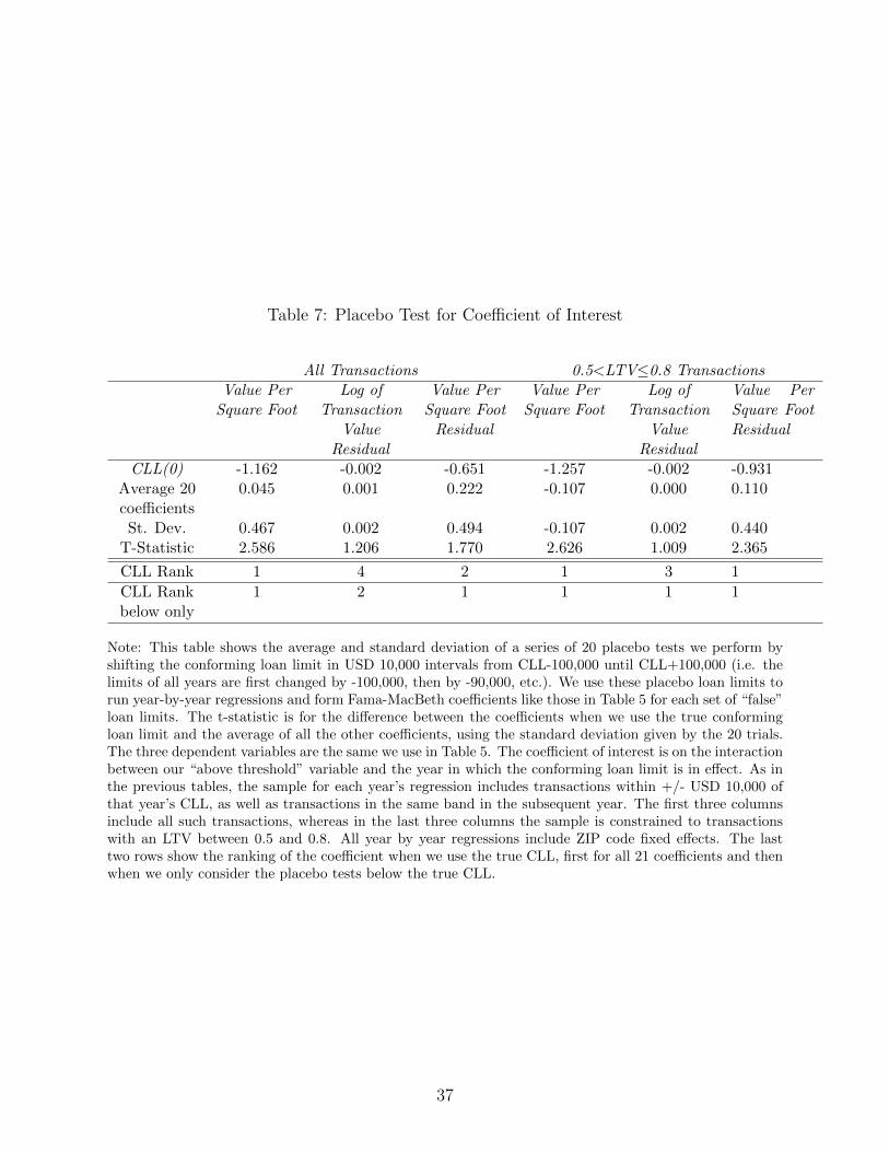
Table 7: Placebo Test for Coefficient of Interest

All Transactions 0.5<LTV≤0.8 TransactionsValue PerSquare Foot

Log ofTransaction

ValueResidual

Value PerSquare FootResidual

Value PerSquare Foot

Log ofTransaction

ValueResidual

Value PerSquare FootResidual

CLL(0) -1.162 -0.002 -0.651 -1.257 -0.002 -0.931Average 20coefficients

0.045 0.001 0.222 -0.107 0.000 0.110

St. Dev. 0.467 0.002 0.494 -0.107 0.002 0.440T-Statistic 2.586 1.206 1.770 2.626 1.009 2.365

CLL Rank 1 4 2 1 3 1

CLL Rankbelow only

1 2 1 1 1 1

Note: This table shows the average and standard deviation of a series of 20 placebo tests we perform byshifting the conforming loan limit in USD 10,000 intervals from CLL-100,000 until CLL+100,000 (i.e. thelimits of all years are first changed by -100,000, then by -90,000, etc.). We use these placebo loan limits torun year-by-year regressions and form Fama-MacBeth coefficients like those in Table 5 for each set of “false”loan limits. The t-statistic is for the difference between the coefficients when we use the true conformingloan limit and the average of all the other coefficients, using the standard deviation given by the 20 trials.The three dependent variables are the same we use in Table 5. The coefficient of interest is on the interactionbetween our “above threshold” variable and the year in which the conforming loan limit is in effect. As inthe previous tables, the sample for each year’s regression includes transactions within +/- USD 10,000 ofthat year’s CLL, as well as transactions in the same band in the subsequent year. The first three columnsinclude all such transactions, whereas in the last three columns the sample is constrained to transactionswith an LTV between 0.5 and 0.8. All year by year regressions include ZIP code fixed effects. The lasttwo rows show the ranking of the coefficient when we use the true CLL, first for all 21 coefficients and thenwhen we only consider the placebo tests below the true CLL.

37

Table 8: Effect of the CLL on the Valuation of Different Groups of Transactions

Panel A: Value Per Square Foot

Keeping Conforming Keeping JumboAll years 1998-2001 2002-2005 All years 1998-2001 2002-2005

Above Threshold 0.939** 1.580*** 0.297 0.868* 1.530*** 0.207(0.472) (0.568) (0.666) (0.481) (0.545) (0.701)

Year CLL -24.539*** -15.953*** -33.126*** -24.874*** -16.040*** -33.708***(4.351) (2.564) (5.712) (4.454) (2.596) (5.813)

Above Threshold x -0.967** -1.314** -0.621 -2.177*** -2.618** -1.736**Year CLL (0.416) (0.572) (0.634) (0.639) (1.119) (0.724)No. Obs. 177,227 72,048 105,179 160,342 62,905 97,437

Panel B: Log of Transaction Value Residual from Hedonic Regressions

Keeping Conforming Keeping JumboAll years 1998-2001 2002-2005 All years 1998-2001 2002-2005

Above Threshold 0.0117*** 0.0145*** 0.0090*** 0.0119*** 0.0146*** 0.0091***(0.0014) (0.0018) (0.0007) (0.0013) (0.0016) (0.0008)

Year CLL 0.0367*** 0.0335*** 0.0398*** 0.0370*** 0.0337*** 0.0402***(0.0038) (0.0041) (0.0067) (0.0039) (0.0042) (0.0068)

Above Threshold x -0.0027** -0.0019 -0.0034*** 0.0004 -0.0020 0.0028**Year CLL (0.0011) (0.0022) (0.0009) (0.0015) (0.0025) (0.0012)No. Obs. 170,808 68,719 102,089 154,848 60,114 94,734

Panel C: Value Per Square Foot Residual from Hedonic Regressions

Keeping Conforming Keeping JumboAll years 1998-2001 2002-2005 All years 1998-2001 2002-2005

Above Threshold 1.573*** 1.947*** 1.199*** 1.583*** 1.991*** 1.175**(0.290) (0.357) (0.414) (0.308) (0.333) (0.470)

Year CLL 3.514*** 3.485*** 3.543*** 3.529*** 3.552*** 3.507***(0.579) (0.431) (1.175) (0.573) (0.409) (1.168)

Above Threshold x -1.399*** -1.216** -1.583*** 0.225 -0.462 0.911**Year CLL (0.344) (0.535) (0.493) (0.418) (0.536) (0.464)No. Obs. 170,946 68,790 102,156 154,949 60,165 94,784

Note: This table shows Fama Macbeth coefficients computed from year by year regressions that use threealternative measures of valuation as the dependent variable in each of the three panels. The hedonicregressions that produce the residuals for panels B and C are described in Section 3.2. The sample foreach year’s regression includes transactions within +/- USD 10,000 of that year’s conforming loan limit.All year by year regressions include ZIP code fixed effects. We divide the transactions that happen at aprice above 125 percent of a year’s CLL in the year that the limit is in effect into two groups: those witha conforming loan and those with a jumbo loan. We then run the same regressions including just one ofthese two groups at a time. The first three columns include the transactions with a conforming loan and thelast three columns include transactions with a jumbo loan. Above the Threshold refers to transactions upto USD 10,000 above the conforming loan limit divided by 0.8 (i.e. the transactions that were “ineligible”to be bought with a conforming loan at a full 80 percent LTV) and Year CLL is the year in which theconforming loan limit is in effect.

38

Table 9: Effect of the CLL on House Valuation in Low Supply Elasticity Areas (Elasticity≤1)

Panel A: Value Per Square Foot

All All 1998-2001 1998-2001 2002-2005 2002-2005Above Threshold 1.261** 1.221 1.669*** 3.069*** 0.852 -0.628

(0.494) (0.799) (0.573) (0.374) (0.836) (0.749)Year CLL -22.869*** -15.282*** -14.851*** -8.015*** -30.886*** -22.550***

(4.047) (3.920) (2.314) (0.843) (5.314) (5.981)Above Threshold x -1.162*** -0.430 -1.553*** -2.100** -0.771** 1.239Year CLL (0.264) (0.831) (0.297) (0.817) (0.369) (0.832)Above Threshold x -0.870 0.726 -2.466**Year CLL x Low Elasticity (0.977) (1.332) (0.992)No. Obs. 262,671 262,671 109,496 109,496 153,175 153,175

Panel B: Log of Transaction Value Residual from Hedonic Regressions

All All 1998-2001 1998-2001 2002-2005 2002-2005Above Threshold 0.0129*** 0.0106*** 0.0154*** 0.0182*** 0.0104*** 0.0030*

(0.0013) (0.0030) (0.0015) (0.0012) (0.0009) (0.0016)Year CLL 0.0387*** 0.0263*** 0.0356*** 0.0306*** 0.0417*** 0.0219***

(0.0041) (0.0037) (0.0047) (0.0044) (0.0072) (0.0055)Above Threshold x -0.0017** 0.0008 -0.0020 -0.0018 -0.0013*** 0.0033*Year CLL (0.0008) (0.0022) (0.0015) (0.0037) (0.0004) (0.0018)Above Threshold x -0.0032 -0.0002 -0.0063***Year CLL x Low Elasticity (0.002) (0.004) (0.0020)No. Obs. 251,431 251,431 103,535 103,535 147,896 147,896

Panel C: Value Per Square Foot Residual from Hedonic Regressions

All All 1998-2001 1998-2001 2002-2005 2002-2005Above Threshold 1.733*** 1.338** 2.060*** 2.623*** 1.407** 0.054

(0.360) (0.524) (0.425) (0.278) (0.595) (0.319)Year CLL 4.103*** 1.811** 3.935*** 3.316*** 4.270*** 0.305

(0.644) (0.716) (0.495) (0.270) (1.293) (0.898)Above Threshold x -0.651*** -0.503 -0.940*** -1.620*** -0.362 0.615Year CLL (0.238) (0.546) (0.351) (0.306) (0.291) (0.684)Above Threshold x -0.241 0.843 -1.325Year CLL x Low Elasticity (0.740) (0.744) (1.104)No. Obs. 251,764 251,764 103,709 103,709 148,055 148,055

Note: In this case the dummy is 1 for low elasticity places. For this specification that corresponde to thelowest MSA ( Miami, San Francisco, San Diego, Los Angeles, New York, Chicago and Boston). The areaswith elasticity higher than 1 are Las Vegas, Denver and DC

39

Table 10: Elasticity Estimates

Jumbo-Conforming Spread∆ House Prices in bp Min (10 bp) Max (24 bp)

Max: 91.2 9.1 3.8Min: 29.7 3.0 1.2

Note: This table shows elasticity calculations for different scenarios of both the house price increase es-timated in the regressions and the interest rate differential implied for transactions above and below thethreshold of 125 percent of the conforming loan limit. We use the jumbo-conforming spread in interest ratesas the denominator in the elasticity calculation.

40