Credit Risk and Market Risk: Analyzing US Credit … Risk and Market Risk: Analyzing US Credit...
59
Credit Risk and Market Risk: Analyzing US Credit Spreads Dr. Hayette Gatfaoui Associate Professor, Rouen School of Management, Economics & Finance Department, 1 Rue du Maréchal Juin, BP 215, 76826 Mont-Saint-Aignan Cedex France; Phone: 00 33 2 32 82 58 21, Fax: 00 33 2 32 82 58 33; [email protected] August 2006 Abstract We attempt to disentangle US credit spreads’ evolution into a part result- ing from market risk influence and a part resulting from default risk influ- ence. We consider twokinds of data, namely credit spreads (versus Treasury yields) as a proxy of credit risk and S&P 500 stock index as a proxy of mar- ket/systematic risk. Such data allow for achieving a sensitivity study of credit risk to systematic risk relative to sector, credit rating and maturity risk lev- els. First, we extract the common unobserved component of credit risk (i.e., common latent factor) from observed credit spread data in the light of three risk dimensions, namely credit rating, maturity and industry. We exhibit then the sensitivity of credit risk to market risk according to three different risk levels, namely the three risk dimensions previously mentioned. Second, we investigate the link prevailing between the common latent factor and S&P 500 stock index along with those three risk dimensions. We exhibit therefore the link prevailing between the systematic component of credit spreads (i.e., credit risk) and S&P 500 index as a proxy of market risk factor. We find that employing S&P 500 stock index as a proxy of the systematic risk component in US credit spreads generates a valuation bias while assessing credit risk. 1
-
Upload
phamkhuong -
Category
Documents
-
view
216 -
download
0
Transcript of Credit Risk and Market Risk: Analyzing US Credit … Risk and Market Risk: Analyzing US Credit...

Credit Risk and Market Risk: Analyzing USCredit Spreads
Dr. Hayette Gatfaoui
Associate Professor, Rouen School of Management,Economics & Finance Department, 1 Rue du Maréchal Juin,
BP 215, 76826 Mont-Saint-Aignan Cedex France;Phone: 00 33 2 32 82 58 21, Fax: 00 33 2 32 82 58 33;
August 2006
Abstract
We attempt to disentangle US credit spreads’ evolution into a part result-ing from market risk influence and a part resulting from default risk influ-ence. We consider two kinds of data, namely credit spreads (versus Treasuryyields) as a proxy of credit risk and S&P 500 stock index as a proxy of mar-ket/systematic risk. Such data allow for achieving a sensitivity study of creditrisk to systematic risk relative to sector, credit rating and maturity risk lev-els. First, we extract the common unobserved component of credit risk (i.e.,common latent factor) from observed credit spread data in the light of threerisk dimensions, namely credit rating, maturity and industry. We exhibitthen the sensitivity of credit risk to market risk according to three differentrisk levels, namely the three risk dimensions previously mentioned. Second,we investigate the link prevailing between the common latent factor and S&P500 stock index along with those three risk dimensions. We exhibit thereforethe link prevailing between the systematic component of credit spreads (i.e.,credit risk) and S&P 500 index as a proxy of market risk factor. We find thatemploying S&P 500 stock index as a proxy of the systematic risk componentin US credit spreads generates a valuation bias while assessing credit risk.
1

Keywords: Credit spreads, Credit risk, Flexible least squares, Kalman filter,Latent factor, Market risk, Systematic risk.
JEL Codes: C32, C51, G1.
1 Introduction
Recent literature focuses on the basic components of credit risk, andmainly the interaction between systematic and idiosyncratic risk in determin-ing credit risk level (see Crouhy, Galai &Mark (1999)). Namely, the influenceof business cycle (that represents the systematic risk factor)1 on credit risk isinvestigated while studying the impact of key macroeconomic indicators. Onone hand, many authors investigated and emphasized the systematic natureand component of credit risk (see Jarrow &Turnbull (1995a,b), Das & Tufano(1996), Duffee (1998), Jarrow & Turnbull (2000), Elton, Gruber, Agrawal &Mann (2001), Hillegeist et al. (2002), Bongini et al. (2002), Allen & Saun-ders (2003), Xie, Wu & Shi (2004), Koopman, Lucas & Klaassen (2005),Dionne et al. (2006)). The obtained results support the significant role ofboth systematic risk and relevant market and/or macroeconomic indicatorsin explaining the level and evolution of credit risk fundamentals. On theother hand, other authors disentangled credit risk into two components suchas systematic/market risk and idiosyncratic/specific risk (see Dichev (1998),Wilson (1998), Nickell et al. (2000), Baraton & Cuillere (2001), Crouhy,Galai & Mark (2000, 2001), Delianedis & Geske (2001), Spahr et al. (2002),Ericsson & Renault (2003), Gatfaoui (2003), Aramov et al. (2004), Gatfaoui(2005), Jarrow, Lando & Yu (2005), Bakshi, Madan & Zhang (2006)). Re-lated issues support that credit risk results from the combination of financialand macroeconomic risk factors (i.e., market and systematic risk factors)with idiosyncratic and firm-specific risk factors (e.g., liquidity risk).2
More recently, various sophisticated latent factor models arose to studythe relationship prevailing between credit risk and market risk, or equiva-lently business cycle (see Galgliardini & Gouriéroux (2004), Koopman, Lu-cas & Daniels (2005)). One-factor models attempt to account for the mar-ket risk side while assessing credit risk (see Cipollini & Missaglia (2005),
1Indeed, the systematic risk factor is usually represented by business conditions sincethis one is highly correlated with macroeconomic fundamentals (see Fama & French (1989)for example).
2See Ericsson & Renault (2003) as well as Driessen (2005) for example.
2

Hamerle, Liebig & Scheule (2004)) whereas multi-factor models focus onobserved and unobserved latent macroeconomic factors (i.e., business cy-cle) underlying credit risk evolution (see Hui, Lo & Huang (2003), Tasche(2005), Berardi & Trova (2005)). Indeed, incorporating latent factors im-proves model accuracy and reliability while assessing credit risk (see Amato& Luisi (2006), Jakubik (2006)). With regard to corporate bonds and creditspreads, Elizalde (2005) shows that credit risk results essentially from com-mon risk factors that affect all firms. Credit risk is decomposed into differentunobservable factors among which a single common factor accounts for morethan 50% of firm credit risk levels. Moreover, this single common factor isstrongly correlated with known US stock market indices. In the same line,Saita (2006) implements a reduced-form latent factor model while studyingcredit spreads versus risk-free rates. The model incorporates macroeconomicvariables as well as firm-specific factors such as leverage and firm volatil-ity. This way, the author shows that expected excess returns on corporatebonds (i.e., credit spreads) depend on systematic risk factors. Namely, un-known and unobserved systematic risk factors in addition to Fama & French(1993) systematic risk factors might explain a large portion of observed creditspreads (i.e., default timing and default event). Studying also corporate bondspreads, Frühwirth, Schneider & Sögner (2005) distinguish between interestrate risk, credit risk (i.e., issuer-specific risk) and liquidity risk (i.e., bond-specific risk). These components are extracted from relevant latent processesthat represent both bond-specific and issuer-specific risk factors. Moreover,the correlation between the risk-free term structure and credit risk is alsotaken into account. Later Berndt, Lookman & Obrega (2006) investigate thelink between default risk premia and both systematic observed risk factorsand an unobserved latent risk factor. Considering unexplained returns (i.e.,that part of corporate bond returns, which does not result from changesin risk-free rates and expected losses), they distinguish between Fama &French (1993) systematic factors (e.g., default and term factors), Jegadeesh& Titman (1993) momentum factor, and an unobserved common latent com-ponent. Moreover, unexplained returns reveal to be independent of defaultprobabilities, credit ratings, leverage ratios and recovery rates. With regardto failure rates, Koopman & Lucas (2005) employ a multivariate unobservedcomponent methodology to investigate the link prevailing between macroeco-nomic conditions and both credit spreads and failure rates. They emphasizeempirically the correlation existing between credit risk and macroeconomicstate. In a similar view, Jakubik (2006) investigates the link between credit
3

risk and business cycle. The author targets the impact of macroeconomicchanges on default events. For microeconomic reasons, the author considersmacro credit risk models that incorporate latent systematic risk factors inorder to predict default rates.In the light of the strong relationship between credit risk and market risk,
we realize a two-stage study while investigating US credit spreads’ evolutions.First, we emphasize the global common component in all credit spreads underconsideration, which represents the systematic part of credit risk at sector-,rating-, and maturity-based levels. We argue that the decomposition of creditspreads into systematic and idiosyncratic components varies across sectors,credit ratings and maturities. Second, we investigate the dynamic link thatprevails between the systematic component in credit spreads and the S&P 500stock index return. We check whether the common practice that resorts toS&P 500 stock market index as a proxy for systematic risk factor is coherent.Specifically, we address three distinct questions. Firstly, can we describe theinteraction arising between credit risk and market risk over time? Secondly,is S&P 500 index a convenient proxy for the financial market when assessingthe systematic component of US credit spreads? Thirdly, when this is notthe case, can we use the link prevailing between credit spreads and S&P 500index to extract or estimate the systematic part of credit spreads?The paper is organized as follows. Section 2 introduces the data and some
related empirical features. Section 3 presents the methodology employedto extract the common latent component in credit spreads in the light ofthree risk dimensions, namely economic sector, credit rating and maturity.Section 4 investigates the link between the common latent component incredit spreads and S&P 500 stock index along with the three previous riskdimensions. Finally, section 5 draws some concluding remarks and proposesfuture research extensions.
2 Data
We introduce the set of data under consideration as well as related timehorizon and specific exhibited features.
4

2.1 Description
We consider monthly data ranging from May 1991 to November 2000,namely a total of 115 observations per series. Those data are extracted fromBloomberg database, and consist of US corporate credit spreads and S&P500 stock market index. US corporate credit spreads are expressed in basispoints. First, credit spreads are computed as the difference between middleaggregate risky bond yields and corresponding Treasury yields. They aresorted by sector, rating and maturity. Indeed, we consider four differentsectors, namely banking and finance (BF), industrials (IN), power (PW)and telecommunications (TL). Moreover, we focus on investment grade riskybonds whose ratings range from AAA to BAA, and are provided by Moody’srating agency. Maturities range from one year to twenty years (when they areavailable) in order to study short term and long term credit risk profiles. Wetherefore consider a total number of 116 credit spread time series all sectors,maturities and ratings included. The whole set of average corporate creditspreads under consideration is listed in table 1.
We focus therefore on the economic trend in US corporate credit spreadsalong with three levels of analysis, namely industry, credit rating and ma-turity. Those three risk level analyses are motivated by empirical findings.Industry distinction is motivated by both the fact that firm characteristicsvary across sectors (see Collin-Dufresne & Goldstein (2001)) and the exis-tence of industry-specific fundamentals (see Wilson (1997a,b)). Credit rat-ings exhibit a strong informational content (see Boot, Milbourn & Schmeits(2006) and Odders-White & Ready (2006)). Namely, credit ratings expressan issuer’s solvency along with macroeconomic risk, commercial risk (e.g.,competitive environment, firm positioning) and financial state (e.g., finan-cial policy and structure, financial flexibility, profitability) concerns. Indeed,Boot, Milbourn & Schmeits (2006) emphasize the substantial and significanteconomic role of credit ratings (i.e., signalling role about firm quality as wellas related creditworthiness for potential investors, and monitoring processof rating agencies) insofar as firms need to act in order to maintain and/orimprove their credit rating. Moreover, credit ratings impact strongly firms’debt levels as well as related capital structures (see Faulkender & Petersen(2005) and Kisgen (2006)). Specifically, Kisgen (2006) shows the immediateimpact of credit ratings on firms’ capital structure decisions. Incidentallyand with regard to credit risk term structure, firm-specific factors as well
5

Table 1: Coporate credit spreads
Maturity (years)Rating 1 2 3 4 5 7 10 20
AAAINBF
INBF
BF ININBF
INBF
INBF
IN
AA2INBFPW
INBF
INBF
INBFPW
INBFPW
INBFPW
AA3INTLPW
INTLPW
INTL
TLINTLPW
INTLPW
TLPW
A1INTLPW
INTL
INTL
INTLPW
INTLPW
INTL
A2INTLPW
INTLPW
INTL
INTLPW
INTLPW
INTLPW
A3INTLPW
INTLPW
INTL
INTLPW
INTLPW
TL
BAA1INTL
INTL
INTL
INTL
INTL
INTL
BAA2 IN IN IN IN INBAA3 IN IN IN IN IN IN
6

as corresponding country’s financial system and institutional traditions (i.e.,regulations and corporate governance) determine the debt maturity struc-ture of a firm (see Antoniou, Guney & Paudyal (2006)). Antoniou, Guney& Paudyal (2006) show a negative link between debt maturity and firm liq-uidity. Specifically, those authors identify market related factors that impactsubstantially any firm’s debt maturity structure. Moreover, Shimko, Tejima& Van Deventer (1993) show that the slope of credit spread term structure(as well as credit spread volatility) depends on the changes in interest ratevolatility (i.e., link with some market-specific fundamental).
Second, we consider the Standard & Poor’s composite index (S&P 500)as a proxy of market/systematic risk factor (i.e., some market portfolio withfive hundreds stocks). Since credit spreads exhibit some yield nature andfor homogeneity purposes, we consider the continuous monthly returns ofS&P 500 index rather than its levels. Namely, according to Fisher (1959),corporate credit spreads and S&P 500 stock index (which is also thought as aproxy of business conditions) should be negatively linked (see also Gatfaoui(2005,2006)) given that we lie in the growth side of the business cycle.3 Tocheck for the coherency of our homogeneity concern, we naively computed thenon-parametric correlation coefficients (i.e., Kendall’s tau and Spearman’srho) between US corporate credit spreads and both S&P 500 levels and S&P500 continuous returns. In unreported results, we found a general positivelink4 between US corporate credit spreads and S&P 500 levels whereas wefound a strong negative link5 between US corporate credit spreads and S&P500 returns. Consequently, our homogeneity concern has a high significanceall the more that it impacts the nature of the results to be obtained as wellas related interpretation and conclusions.
2.2 Empirical features
We underline and exhibit some statistical features of the data underconsideration. First, in unreported results, we ran a Phillips & Perron sta-tionarity test at a one percent level and found that S&P 500 index returns are
3Generally speaking, this negative link means that an increase of systematic risk im-pacts negatively credit risk. Specifically, a decrease in S&P 500 returns generates a widen-ing of corporate credit spreads.
4An extremely small number of computed non-parametric correlation coefficients arenegative.
5All the non-parametric correlation coefficients that were computed are negative.
7

Table 2: Median industrial credit spreads in basis points
1Y 2Y 3Y 4Y 5Y 7Y 10Y 20Y
AAA 38.0000 32.0000 30.0000 32.0000 31.0000 34.0000 35.0000
AA2 44.0000 37.0000 36.5000 37.0000 38.0000 40.0000
AA3 49.0000 40.0000 41.0000 40.0000 42.0000
A1 56.0000 46.0000 50.0000 49.0000 50.0000 53.0000
A2 64.0000 52.0000 56.5000 63.0000 63.0000 64.0000
A3 73.0000 61.0000 62.5000 69.0000 68.0000
BAA1 84.0000 77.0000 74.5000 78.0000 79.0000 80.0000
BAA2 93.0000 85.0000 82.5000 85.0000 89.0000
BAA3 109.0000 99.0000 96.5000 97.0000 111.0000 118.0000
Table 3: Skewness of industrial credit spreads
1Y 2Y 3Y 4Y 5Y 7Y 10Y 20Y
AAA 0.0054 0.5061 1.5554 1.7469 1.9563 1.7289 1.5088
AA2 0.6544 0.6393 1.1702 1.9193 2.0665 1.7625
AA3 0.6825 0.5117 0.8781 1.6205 1.8942
A1 0.7014 0.4280 0.4542 1.2040 1.5011 1.3681
A2 0.4606 0.4594 0.3972 0.8440 1.4213 1.3343
A3 0.3265 0.2956 0.4108 0.9510 1.3384
BAA1 0.3486 0.2885 0.3299 0.7359 1.0474 1.1591
BAA2 0.2805 0.1336 0.2475 0.5195 1.0095
BAA3 0.5921 0.4957 0.4105 0.3317 0.4640 0.4953
stationary whereas US corporate credit spreads are non-stationary. Specifi-cally, credit spreads reveal to be first order integrated time series. Second, wecomputed some descriptive statistics such as median, skewness and kurtosisfor our credit spreads and S&P 500 stock index. Related results are displayedfor each sector and listed in tables 2 to 14.
We therefore consider asymmetric and non-normal data. As regards S&P500 index return, this stock market index return is positively skewed andexhibits a positive excess kurtosis as compared the ones of the Gaussian dis-tribution. As regards US corporate credit spreads, they exhibit the followingstatistical features whatever the credit spread under consideration. As func-tions of rating grades, median corporate credit spreads decrease when thecorresponding credit rating improves. As functions of maturity, median cor-
8

Table 4: Excess kurtosis for industrial credit spreads
1Y 2Y 3Y 4Y 5Y 7Y 10Y 20Y
AAA -0.6695 -0.0700 2.6838 3.4048 4.3448 2.6663 1.9876
AA2 -0.2953 -0.4372 0.8140 3.6516 4.3380 2.8339
AA3 -0.4172 -0.7691 -0.2185 2.2742 3.5721
A1 -0.2116 -1.1199 -0.9971 1.0406 2.2640 1.7285
A2 -0.6324 -1.0974 -1.0632 0.1875 2.0272 1.5532
A3 -0.9194 -1.3706 -1.1146 0.3473 2.0272
BAA1 -1.0692 -1.2390 -1.1264 -0.2857 0.5366 0.6907
BAA2 -1.1085 -1.4962 -1.3784 -0.8617 0.2631
BAA3 -0.7828 -0.9299 -1.1445 -1.3095 -1.0121 -0.8430
Table 5: Median banking and finance credit spreads in basis points
1Y 2Y 3Y 5Y 7Y 10Y
AAA 41.0000 36.0000 36.5000 39.0000 44.0000 46.0000
AA2 50.0000 42.0000 43.5000 50.0000 54.0000 55.0000
Table 6: Skewness of banking and finance credit spreads
1Y 2Y 3Y 5Y 7Y 10Y
AAA 0.0771 0.5160 0.8497 1.0151 1.1624 0.9990
AA2 0.4046 0.6222 0.8230 1.2061 1.3692 1.3074
Table 7: Excess kurtosis for banking and finance credit spreads
1Y 2Y 3Y 5Y 7Y 10Y
AAA -0.0602 -0.4785 -0.1975 0.2643 0.6604 -0.1717
AA2 -0.4766 -0.6893 -0.4021 0.9498 1.2868 0.9199
Table 8: Median telecommunication credit spreads in basis points
1Y 2Y 3Y 4Y 5Y 7Y 10Y
AA3 50.0000 40.0000 40.5000 38.0000 40.0000 42.0000 44.0000
A1 59.0000 49.0000 49.5000 46.0000 49.0000 52.0000
A2 63.0000 56.0000 54.0000 51.0000 54.0000 53.0000
A3 68.0000 61.0000 59.5000 56.0000 59.0000 59.0000
BAA1 74.0000 68.0000 67.0000 67.0000 66.0000 69.0000
9

Table 9: Skewness of telecommunication credit spreads
1Y 2Y 3Y 4Y 5Y 7Y 10Y
AA3 0.1733 0.7575 1.3812 1.5304 1.7811 1.8314 1.8297
A1 0.0221 0.4899 1.1382 1.8101 1.8616 1.8088
A2 0.3913 0.5998 1.4356 1.9565 2.0339 1.8950
A3 0.0221 0.4899 1.1382 1.8101 1.8616 1.8088
BAA1 0.5030 0.4089 1.0116 1.5206 1.4555 1.4698
Table 10: Excess kurtosis for telecommunication credit spreads
1Y 2Y 3Y 4Y 5Y 7Y 10Y
AA3 -0.8179 -0.2833 1.3247 2.2035 2.6105 3.0903 2.7696
A1 -0.9156 -0.2947 0.9891 2.8846 3.3375 2.8933
A2 -0.6124 0.2381 2.2776 3.6817 4.1023 3.3160
A3 -0.9156 -0.2947 0.9891 2.8846 3.3375 2.8933
BAA1 -0.6092 -0.7629 0.5492 2.0590 1.8260 1.8475
Table 11: Median power credit spreads in basis points
1Y 2Y 5Y 7Y 10Y
AA2 45.0000 36.0000 40.0000 44.0000
AA3 55.0000 44.0000 41.0000 45.0000 47.0000
A1 62.0000 47.0000 50.0000
A2 66.0000 52.0000 52.0000 55.0000 58.0000
A3 72.0000 57.0000 58.0000 62.0000
Table 12: Skewness of power credit spreads
1Y 2Y 5Y 7Y 10Y
AA2 0.3751 1.7064 1.8879 1.5682
AA3 0.0983 0.7859 1.7813 1.9007 1.5888
A1 0.0828 1.8710 1.9887
A2 -0.0158 0.8360 1.7872 1.9017 1.7093
A3 0.0771 0.6016 1.7624 1.8828
10

Table 13: Excess kurtosis for power credit spreads
1Y 2Y 5Y 7Y 10Y
AA2 -0.3843 2.5288 3.2178 1.8704
AA3 -1.1282 0.0435 2.6298 3.3824 1.9500
A1 -1.0025 2.8878 3.6656
A2 -1.0718 -0.0637 2.6025 3.2532 2.3077
A3 -0.8979 -0.5393 2.6901 3.2519
Table 14: Descriptive statistics for Standard and Poor’s 500 stock index
Level Return (bps)
Median 645.3000 83.7925
Skewness 0.6585 0.1873
Excess kurtosis -1.0973 1.4405
porate credit spreads tighten until two-, three- or four-year maturities, andthen widen as maturity increases. Such a behavior doesn’t apply to telecom-munication credit spreads whose behaviors are farther more irregular as func-tions of maturity. Moreover, corporate credit spreads are generally positivelyskewed (i.e., right-skewed, or equivalently with a fat right-tail). Hence, overour studied time horizon, we face substantial numbers of credit spreads ly-ing above their related average values (i.e., substantial risk of high creditspreads as compared to their corresponding average levels). Finally and gen-erally speaking, their corresponding excess kurtosis is usually negative formaturities below four years (below two years for the telecommunication sec-tor) whereas it becomes positive for other higher maturities except for thelowest rating grades of industrial and power sectors.
3 Latent systematic factor
Recent literature employs observed macroeconomic variables to exhibitthe correlation of default indicators across firms as well as industries (seeGersbach & Lipponer (2003)6). According to related empirical issues, macro-economic factors reveal to be insufficient while assessing credit risk insofar as
6Those authors exhibit the impact of macroeconomic shocks on both default probabil-ities and default correlations. They find that default correlations may explain more thanfifty percent of credit risk increase in case of adverse macroeconomic shocks.
11

additional latent risk factors need to be considered. To bypass such an issue,we gather any observed and unobserved common financial, economic andmacro component describing credit risk fundamentals (e.g., credit spreads)into one global common unobserved latent factor. Our motivation comesfrom Collin-Dufresne et al. (2001) who show that credit spreads’ changes aremainly driven by a common latent factor in corporate bonds. We then resortto a specific econometric tool to exhibit such a common latent component incorporate credit spreads, namely Kalman linear filter methodology.
3.1 Methodology
Kalman filter (see Kalman (1960), Brown & Hwang (1997), and Cressie& Wikle (2002)) is a state-space representation that allows for consideringan unobserved variable (i.e., a state variable), which is estimated with theobservable model (i.e., observed variables or measures). Specifically, Kalmanfilter attempts to estimate a state variable (e.g., the common latent compo-nent in credit spreads) given disturbed observations about the correspondingsystem (e.g., observed corporate credit spreads).7 Indeed, observed measures(i.e., corporate credit spreads) are functions of the state variable (i.e., thestate of the system, or equivalently the unobserved common component incorporate credit spreads) insofar as the considered measures are disturbedby a random noise called measurement noise. The main advantage is thatsuch an econometric method can be applied to stationary as well as non-stationary data.8 Moreover, we do not need a proxy for business conditionsor systematic risk factor, this unobserved risk component being inferred fromKalman filter.We consider that our state variable, namely the common latent compo-
nent in credit spreads, follows a first order Markov process. And, we considerthe following linear measurement equation (Equation 1) and state (i.e., dy-namic/transition) equation (Equation 2):
CSt = α ·Mt + et (1)
7More precisely, Kalman filter attempts to estimate the common latent component ateach time t conditional on observed corporate credit spreads until time t. This methodol-ogy minimizes realized squared errors on the common latent component in credit spreads(i.e., quadratic minimization algorithm).
8Recall that S&P 500 index returns are stationary whereas corporate credit spreadsare non-stationary.
12

Mt = αM Mt−1 + wt (2)
with CSt =
⎡⎢⎣ CS1t...
CSNt
⎤⎥⎦, α =
⎡⎢⎣ α1...αN
⎤⎥⎦, and et =
⎡⎢⎣ e1t...eNt
⎤⎥⎦. First, N depends
on the analysis level, namely sector-, rating- or maturity-based analysis,9
and time t ranges from 1 to 115. Second, CSt represents the set of creditspreads under consideration (i.e., observed variables/measure variables), αis a vector that represents the sensitivity of credit spreads to the commonlatent component Mt (i.e., state variable or hidden/unobserved variable), etis a measurement error that represents the unsystematic/idiosyncratic creditspread component, αM is a state transition scalar and wt is a state error(i.e., transition/dynamic error) that may represent market-specific anomaliesor market-specific liquidity effects. Moreover, we assume that (et) and (wt)are independent Gaussian white noises. Third, we consider a causal andinvertible state-space model such that:µ
etwt
¶v N
µ∙0
0
¸,
∙Ht 00 Qt
¸¶andM0 v N (m0, P0) where N (·) is the Gaussian distribution,m0 and P0 areknown state expectation and variance parameters,10 Ht is the measurementerror covariance matrix and Qt is the state variance parameter. Incidentally,we also assume a stationary setting such that α, αM , Ht and Qt are indepen-dent of time t (i.e., Ht and Qt take the same value whatever the time point tunder consideration). We furthermore make the following complementary as-sumptions. As a first step, state variance parameters P0 and Qt = σ2
M are setto take distinct and different values. As a second step, Ht = Diag [σ2
i ]1≤i≤Nis a diagonal N×N covariance matrix. Whatever the analysis level (i.e., sec-tor, rating and industry), Kalman methodology allows then for decomposing
9At a sector level, N is successively 52, 12, 31 and 21 for IN, BF, TL and PW sectorsrespectively. At a rating level, N is successively 12, 5, 6, 15, 17, 15, 16, 17 and 13 forBAA1, BAA2, BAA3, A1, A2, A3, AA2, AA3 and AAA rating grades respectively. At amaturity level, N is successively 21, 19, 15, 2, 21, 20, 17 and 1 for 1, 2, 3, 4, 5, 7, 10 and20-year maturities respectively.10We emphasize the fact that M0 is independent of both (et) and (wt). Moreover, M0
represents the initial state of the system, or equivalently the initial value of the commonlatent factor that we need to guess.
13

a set of credit spreads into a systematic latent component (i.e., common un-observed factor) and an idiosyncratic (i.e., unsystematic) component, whichis peculiar to each credit spread under consideration in the light of the chosenanalysis level.Consequently, running our state-space representation requires the estima-
tion of 2N + 4 parameters, namely measure-specific sensitivity parametersα, state transition parameter αM , initial value M0 of the common latentcomponent (i.e., initial state of the system), diagonal covariance matrix Ht
composed of N elements, variance P0 of the initial value of the commonlatent component, and state variance parameter σ2
M . Under normality as-sumptions, CSt follows a multivariate normal law conditional onMt and pastvalues of both latent factorM and related credit spreads CS. Therefore, im-plementing Kalman methodology leads to maximize the log-likelihood of theconditional distribution of CSt.
Using Kalman filter methodology will then help make an inventory of andrank the sensitivity levels of credit spreads to the common latent component(i.e., unobserved systematic factor) as functions of credit rating, maturityand industry. Those sensitivity levels focus on the extent to which creditspreads tend to evolve together (i.e., the degree of instantaneous link orcorrelation) over time in the light of their respective industry, rating andmaturity. Such a concern is of high significance for credit risk managers (seeWilson (1998)). Indeed, diversified credit portfolios usually bear the commonrisk component in their corresponding constituent credit risky assets. Sincethe idiosyncratic risk component of their credit portfolios is diversified away,credit risk managers focus on the related residual systematic risk component(i.e., correlation risk of credit risky assets or credit lines). Moreover, diversi-fication needs to be envisioned in the light of asset-specific and sector-specificfeatures among others.
3.2 Econometric results
We realize a three-stage study while trying to understand and high-light the common evolution trend that drives US corporate credit spreads.First, we investigate a common component in credit spreads at a sector level.For each sector, we extract the common systematic risk component in creditspreads while considering all available maturities and rating grades. We thenexhibit the unobserved systematic risk component in sector credit risk. Sec-
14

ond, we investigate a common component in credit spreads at a rating gradelevel. For each rating grade, we extract the common systematic risk compo-nent in credit spreads while considering all available maturities and sectors.We then exhibit the unobserved systematic risk component in credit risk asa function of rating grades. Third, we investigate a common component incredit spreads at a maturity level. For each maturity, we extract the commonsystematic risk component in credit spreads while considering all availablesectors and rating grades. We therefore exhibit the unobserved systematicrisk component in credit risk as a function of maturity.
We undertake our state-space model estimation while employing a Broyden-Fletcher-Goldfarb-Shano optimization algorithm. Corresponding relative gra-dients are computed with an accuracy level of 6 digits. Related significantKalman results are given in the appendix. We just summarize briefly theobtained results. With regard to the sector level and whatever the industryunder consideration, corresponding α estimates lie between 1.7 and 4 for BF,TL and PW sectors whereas they lie between 2 and 6 for IN industry. Theseestimates are all significant at a one percent Student test level for BF, TLand IN whereas they are significant at a ten percent test level for BF sector.The same conclusion applies to related standard deviations. Given that αestimates are positive and above unity, credit spreads tend then to magnifythe shocks on the corresponding sector-specific common latent componentsover time (i.e., they magnify systematic sector-specific shocks). Moreover,Qt, M0 and αM coefficients are significant for the corresponding respectiveStudent test levels whereas P0 is insignificant. With regard to the ratinglevel and whatever the credit rating under consideration, corresponding αestimates lie between 1.6 and 5. These estimates as well as related standarddeviations are all significant at a one percent Student test level except forA2 rating grade case whose significance level is five percent. Hence, creditspreads magnify the shocks on the related common latent component Mt
as a function of credit rating grades (i.e., they magnify systematic rating-based shocks). Moreover, Qt, M0 and αM coefficients are significant at a onepercent Student test level whereas P0 is insignificant. With regard to the ma-turity level and whatever the maturity under consideration, correspondingα estimates lie generally between 1.4 and 4 except for four- and twenty-yearmaturities for which these estimates lie between 5 and 6. These estimatesas well as related standard deviations are all significant at a one percentStudent test level. Then, credit spreads magnify the shocks on the related
15

Table 15: Descriptive statistics for sector-based common latent factors
IN BF TL PWMedian 10.0409 19.5821 21.9827 18.8570
Standard deviation 4.0155 8.2560 9.9231 9.0311Skewness 0.2896 1.1041 1.7510 1.9027
Excess kurtosis -1.3149 0.2772 2.8277 3.0994
Table 16: Descriptive statistics for rating-based common latent factors
Rating Median Standard deviation Skewness Excess kurtosisAAA 15.9781 7.0866 1.3159 0.9249AA2 16.2693 6.8280 1.4483 1.5218AA3 19.5355 9.9622 1.8304 2.7864A1 20.0947 8.5697 1.6270 2.3761A2 26.9554 10.5694 1.4620 2.0131A3 23.3196 8.7974 1.2459 1.2935BAA1 27.1664 10.4231 0.9789 0.3716BAA2 18.1252 7.2284 0.2289 -1.4101BAA3 30.6017 13.0718 0.3255 -1.3107
common latent component Mt as a function of maturity (i.e., they magnifysystematic maturity-based shocks). Moreover, Qt, M0 and αM coefficientsare significant at a one percent Student test level whereas P0 is insignificant.
The results we get with regard to common latent components in corporateUS credit spreads as functions of credit rating, maturity and industry arelisted below from table 15 to table 17.
The median sector-specific common latent factor (i.e., the median valueof the systematic sector-specific part in credit spreads, or equivalently themedian value of the common latent factor in credit spreads that is peculiarto each sector) is the highest for TL sector and the lowest for IN sector.Sector-specific common latent factors (i.e., systematic sector-specific com-ponents in credit spreads) are all positively skewed and exhibit generallya positive excess kurtosis except for IN systematic factor (i.e., IN commonlatent factor).
The median rating-based common latent factor (i.e., the median value of
16

Table 17: Descriptive statistics for maturity-based common latent factors
Maturity Median Standard deviation Skewness Excess kurtosis1Y 30.0761 11.8101 0.2860 -1.31892Y 22.1591 8.1722 1.1645 1.03973Y 13.0737 4.7913 0.9922 0.16874Y 9.5369 3.9492 1.3082 1.10955Y 22.7591 9.3145 1.3937 1.47127Y 18.7156 9.4556 1.9680 3.542910Y 15.0847 7.0048 1.8651 2.954920Y 9.3821 6.0739 1.5973 1.9725
the systematic rating-based part in credit spreads, or equivalently the medianvalue of the common latent factor in credit spreads that is peculiar to eachcredit rating grade) is the highest for BAA3 grade and the lowest for AAAgrade. Moreover, median values of rating-based common latent factors incredit spreads are a non-monotonous function of rating grades. Rating-basedcommon latent factors (i.e., systematic rating-based components in creditspreads) are all positively skewed and exhibit generally a positive excesskurtosis except for BAA3 and BAA2 systematic factors (i.e., BAA3 andBAA2 common latent factors).
The median maturity-based common latent factor (i.e., the median valueof the systematic maturity-based part in credit spreads, or equivalently themedian value of the common latent factor in credit spreads that is pecu-liar to each maturity) is the highest for one-year maturity and the lowestfor twenty-year maturity. Moreover, median values of maturity-based com-mon latent factors in credit spreads are a non-monotonous function of ma-turity. However, short term/medium and long term credit spreads exhibit ahigher/lower systematic maturity-based component respectively.11 Maturity-based common latent factors (i.e., systematic maturity-based components incredit spreads) are all positively skewed and exhibit generally a positive ex-cess kurtosis except for the one-year systematic factor (i.e., the one-yearcommon latent factor).
11In unreported results, we notice that the one-year systematic factor in credit spreadsexhibits generally the highest level over time whereas both four-year and twenty-yearsystematic factors in credit spreads behave globally in the same way and exhibit the samelevels over time.
17

0
10
20
30
40
50
60
70
05/31
/1991
09/30
/1991
01/31
/1992
05/29
/1992
09/30
/1992
01/29
/1993
05/31
/1993
09/30
/1993
01/31
/1994
05/31
/1994
09/30
/1994
01/31
/1995
05/31
/1995
09/29
/1995
01/31
/1996
05/31
/1996
09/30
/1996
01/31
/1997
05/30
/1997
09/30
/1997
01/30
/1998
05/29
/1998
09/30
/1998
01/29
/1999
05/31
/1999
09/30
/1999
01/31
/2000
05/31
/2000
09/29
/2000
DateIN BF TL PW
Late
nt fa
ctor
(bps
)
Figure 1: Sector-specific common latent factors in credit spreads
To get a general view, we also plot the levels of the common latent factorswe obtained after running Kalman filter as functions of sector, credit ratingand maturity (see figures 1 to 3).
Previous plots summarize the preliminary results displayed in tables 15to 17. First, IN sector exhibits the lowest systematic credit spread com-ponent over time (i.e., lowest sensitivity to market risk at a sector level)whereas TL sector usually exhibits the highest one as compared to othersector-specific systematic credit spread components. Second, BAA3 system-atic credit spread component is generally the highest over our time horizon(i.e., highest sensitivity to market risk at a credit rating level). Until 1994,AAA and AA2 systematic credit spread components are the lowest whereasBAA2 systematic credit spread component becomes generally the lowest af-ter 1994 as compared to other rating-based systematic credit spread compo-nents. Third, the one-year systematic credit spread component is generallythe highest over our time horizon (i.e., highest sensitivity to market risk ata maturity level). Until 1997, both four-year and twenty-year systematiccredit spread components are the lowest whereas only twenty-year system-atic credit spread component remains the lowest after 1997 as compared to
18

0
10
20
30
40
50
60
70
80
05/3
1/19
91
09/3
0/19
91
01/3
1/19
92
05/2
9/19
92
09/3
0/19
92
01/2
9/19
93
05/3
1/19
93
09/3
0/19
93
01/3
1/19
94
05/3
1/19
94
09/3
0/19
94
01/3
1/19
95
05/3
1/19
95
09/2
9/19
95
01/3
1/19
96
05/3
1/19
96
09/3
0/19
96
01/3
1/19
97
05/3
0/19
97
09/3
0/19
97
01/3
0/19
98
05/2
9/19
98
09/3
0/19
98
01/2
9/19
99
05/3
1/19
99
09/3
0/19
99
01/3
1/20
00
05/3
1/20
00
09/2
9/20
00
Date
BAA3
BAA2
BAA1
A3
A2
A1
AA3
AA2
AAA
Late
nt fa
ctor
(bps
)
Figure 2: Rating-based common latent factors in credit spreads
0
10
20
30
40
50
60
70
05/3
1/19
91
09/3
0/19
91
01/3
1/19
92
05/2
9/19
92
09/3
0/19
92
01/2
9/19
93
05/3
1/19
93
09/3
0/19
93
01/3
1/19
94
05/3
1/19
94
09/3
0/19
94
01/3
1/19
95
05/3
1/19
95
09/2
9/19
95
01/3
1/19
96
05/3
1/19
96
09/3
0/19
96
01/3
1/19
97
05/3
0/19
97
09/3
0/19
97
01/3
0/19
98
05/2
9/19
98
09/3
0/19
98
01/2
9/19
99
05/3
1/19
99
09/3
0/19
99
01/3
1/20
00
05/3
1/20
00
09/2
9/20
00
Date
1Y
2Y
3Y
4Y
5Y
7Y
10Y
20Y
Late
nt fa
ctor
(bps
)
Figure 3: Maturity-based common latent factors in credit spreads
19

other maturity-based systematic credit spread components. Finally, what-ever the sensitivity analysis level, namely sector, credit rating or maturity,corresponding common latent factors (i.e., systematic credit spread compo-nents as functions of sector, credit rating and maturity) exhibit a U-shapedbehavior over our time horizon. We notice a monotonous increase of theirrespective levels from mid-1997 to the end of our time horizon (November2000, which coincides with the end of the business cycle growth trend). Re-call that we faced many economic events and financial facts during this timeperiod. Indeed, we faced the Asian crisis in 1997, the Russian default as wellas LTCM hedge fund collapse in 1998, the shortage of US Treasury bonds dueto massive buybacks as well as the beginning of flight-to-quality phenomenonon bonds in 1999/2000, and finally the multimedia bubble burst in 2000.12
Such events support the widening of credit spreads due to a deteriorationof both systematic risk and/or default risk (and therefore a degradation ofcredit risk).
In unreported results, we computed also the unsystematic credit spreadcomponents corresponding to related sector-, credit rating- and maturity-based systematic components in US corporate credit spreads. The percentageof unsystematic risk components in credit spreads at sector, rating and ma-turity levels lies on average between 29.0041, 15.4545, 16.0915 and 78.4485,72.7654, 71.2222 percent respectively. To get a view, we plot in figures 4 to6 corresponding median values as well as related standard deviations.
At a sector risk level (see figure 4), the median value of the unsystematiccredit spread component decreases when rating quality increases, and it alsoincreases with maturity. Moreover, median values of unsystematic sector-specific credit spread components are generally the highest for IN sector.At a rating risk level (see figure 5), the median value of the unsystematiccredit spread component increases with maturity. At a maturity risk level(see figure 6), the median value of the unsystematic credit spread componentincreases with both rating quality and maturity. The sector-, rating- andmaturity-based unsystematic components in credit spreads have some sig-nificance insofar as they capture the default components (i.e., issuer-specificrisk) as well as liquidity shocks on (i.e., bond-specific risk of) US corporatecredit spreads. Such components are not encompassed in systematic factors.
12From November 1999 to April 2000, internet unlocked share values became aroundfour times higher (see Ofek & Richardson (2003)).
20

0,0000
10,0000
20,0000
30,0000
40,0000
50,0000
60,0000
70,0000
80,0000
90,0000
100,0000
IN01
YBA
A1
IN07
YBA
A1
IN03
YBA
A2
IN02
YBA
A3
IN10
YBA
A3
IN05
YA1
IN
02Y
A2
IN10
YA2
IN
05Y
A3
IN03
YA
A2
IN01
YA
A3
IN07
YA
A3
IN05
YAA
A BF
01Y
AA2
BF
07Y
AA2
B
F03Y
AAA
TL01
YBA
A1
TL07
YBA
A1
TL03
YA1
TL
01Y
A2
TL07
YA2
TL
03Y
A3
TL01
YAA3
TL
05YA
A3
PW
05Y
A1
PW
05Y
A2
PW
02Y
A3
PW05
YAA2
PW
02YA
A3
Credit spreads by sector
Med
ian
(%)
0,0000
10,0000
20,0000
30,0000
40,0000
50,0000
60,0000
Stan
dard
dev
iatio
n
Median Std dev.
Figure 4: Unsystematic sector-specific components in credit spreads
0,0000
10,0000
20,0000
30,0000
40,0000
50,0000
60,0000
70,0000
80,0000
90,0000
IN01
YBAA3
IN10
YBAA3
IN10
YBAA2
IN07
YBAA1
TL05Y
BAA1
IN03
YA3
TL03Y
A3
PW02YA3
IN03
YA2
TL02Y
A2
PW01YA2
IN01
YA1
IN10
YA1
TL07Y
A1
IN01
YAA3
TL01Y
AA3
TL07Y
AA3
PW07YAA3
IN05
YAA2
BF03YAA2
PW05YAA2
IN04
YAAA
BF01YAAA
BF10YAAA
Credit spreads by rating
Med
ian
(%)
0,0000
5,0000
10,0000
15,0000
20,0000
25,0000
30,0000
35,0000
40,0000
45,0000
50,0000
Stan
dard
dev
iatio
n
Median Std dev.
Figure 5: Unsystematic rating-based components in credit spreads
21
0
10
20
30
40
50
60
70
80
90
100
IN01
YBAA3
IN01
YA2
IN01
YAAA
TL01Y
A3
PW01YA3
PW01YAA2
IN02
YA3
IN02
YAA2
TL02Y
BAA1
TL02Y
AA3
IN03
YBAA3
IN03
YA2
BF03YAA2
TL03Y
A2
TL04Y
AA3
IN05
YA3
IN05
YAA2
TL05Y
BAA1
TL05Y
AA3
PW05YAA3
IN07
YA3
IN07
YAA2
TL07Y
BAA1
TL07Y
AA3
PW07YAA3
IN10
YBAA1
IN10
YAAA
TL10Y
A3
PW10YA2
Credit spreads by maturity
Med
ian
(%)
0
5
10
15
20
25
30
35
40
45
50
Stan
dard
dev
iatio
n
Median Std dev.
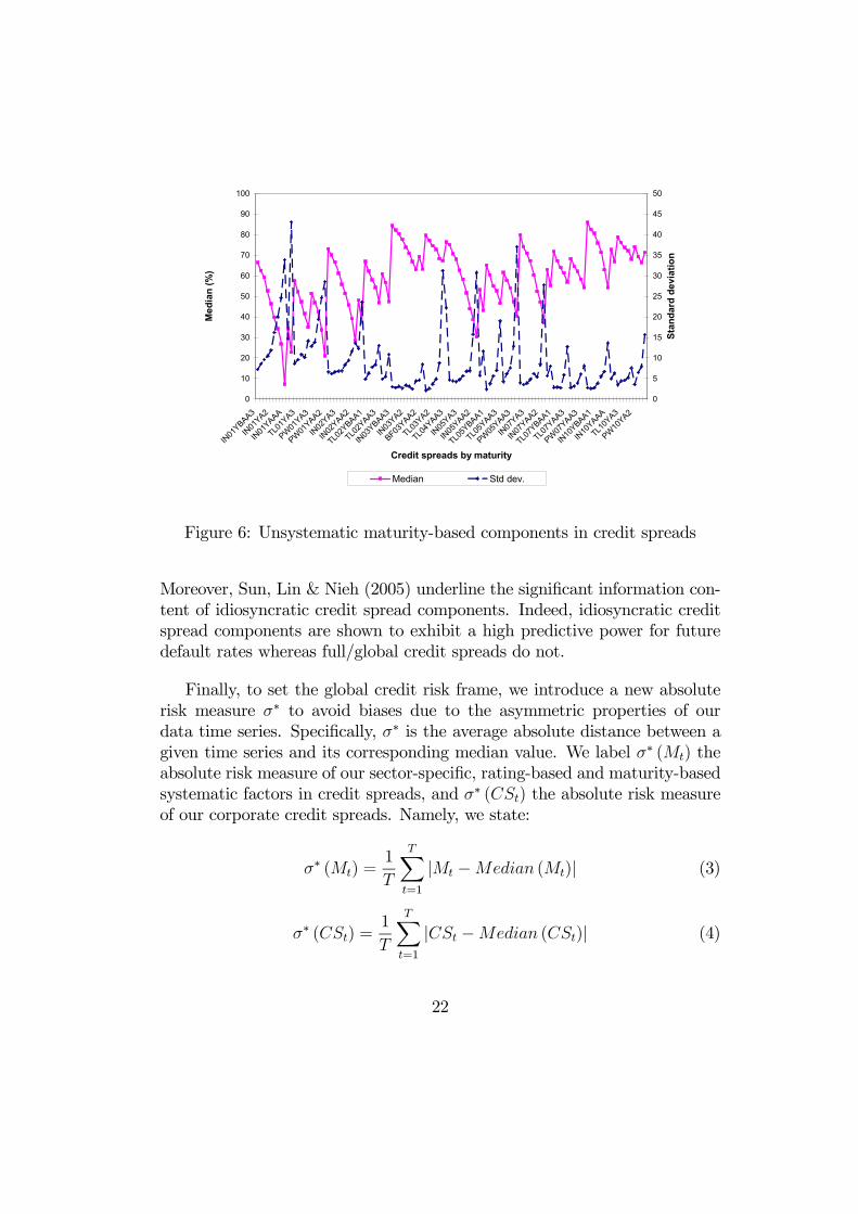
Figure 6: Unsystematic maturity-based components in credit spreads
Moreover, Sun, Lin & Nieh (2005) underline the significant information con-tent of idiosyncratic credit spread components. Indeed, idiosyncratic creditspread components are shown to exhibit a high predictive power for futuredefault rates whereas full/global credit spreads do not.
Finally, to set the global credit risk frame, we introduce a new absoluterisk measure σ∗ to avoid biases due to the asymmetric properties of ourdata time series. Specifically, σ∗ is the average absolute distance between agiven time series and its corresponding median value. We label σ∗ (Mt) theabsolute risk measure of our sector-specific, rating-based and maturity-basedsystematic factors in credit spreads, and σ∗ (CSt) the absolute risk measureof our corporate credit spreads. Namely, we state:
σ∗ (Mt) =1
T
TXt=1
|Mt −Median (Mt)| (3)
σ∗ (CSt) =1
T
TXt=1
|CSt −Median (CSt)| (4)
22

Table 18: Average absolute sector risk measure in basis points
IN BF TL PWσ∗ (Mt) 3.6573 6.2651 6.7748 5.6385
Table 19: Average absolute rating-based risk measure in basis points
BAA3 BAA2 BAA1 A3 A2 A1 AA3 AA2 AAA
σ∗ (Mt) 11.9434 6.6287 8.3943 6.7812 7.7393 5.9280 6.2911 4.8408 5.0737
Hence, σ∗ (CSt) represents some average global credit risk distance (as com-pared to some median credit spread value) whereas σ∗ (Mt) represents someaverage systematic credit risk distance.13 Arguably, such a specificationhelps account for credit spread distribution as well as impact of relatedhigh/extreme values.14 Corresponding absolute risk values are given in tables18 to 20 for systematic credit risk factors as functions of sector, rating andmaturity.15
At sector, rating and maturity levels, the average systematic absolute riskmeasure is the lowest for IN sector, AA2 rating grade, and four-year maturityrespectively. In the same way, the average systematic absolute risk measureis the highest for TL sector, BAA3 rating grade, and one-year maturity. Toget a global view, we also compute the proportion of systematic credit riskin the global credit risk level as p = σ∗(Mt)
σ∗(CSt)× 100. Hence, p represents a
systematic credit risk measure (as compared to some global credit risk level).Related average values are also given in table 21 for each sensitivity analysislevel, namely sector, rating and maturity.16
13Recall that our data are expressed in basis points.14Analogously, we introduce in the appendix other median-related/modified descriptive
statistics such as modified standard deviation, skewness and kurtosis.15To spare space, we do not provide credit spread-related results, which require to display
three times 116 values (i.e., for sector, rating and maturity analysis levels).16At each sensitivity analysis level (i.e., sector, rating and maturity), we compute first
proportion p for each available credit spread data, and we compute then the related arith-
Table 20: Average absolute maturity-based risk measure in basis points
1Y 2Y 3Y 4Y 5Y 7Y 10Y 20Y
σ∗ (Mt) 10.7651 6.4240 3.7684 2.9124 6.8559 5.9461 4.4192 4.0739
23

Table 21: Average systematic risk by sector, rating and maturity in percent
Sector Rating Maturityp 30.2765 37.4996 38.1275
0
5
10
15
20
25
30
35
40
45
50
IN01
YBAA1
IN07
YBAA1
IN03
YBAA2
IN02
YBAA3
IN10
YBAA3
IN05
YA1
IN02
YA2
IN10
YA2
IN05
YA3
IN03
YAA2
IN01
YAA3
IN07
YAA3
IN05
YAAA
BF01YAA2
BF07YAA2
BF03YAAA
TL01Y
BAA1
TL07Y
BAA1
TL03Y
A1
TL01Y
A2
TL07Y
A2
TL03Y
A3
TL01Y
AA3
TL05Y
AA3
PW05
YA1
PW05
YA2
PW02
YA3
PW05
YAA2
PW02
YAA3
Credit spreads by sector
Cre
dit r
isk
(leve
l)
0
10
20
30
40
50
60
Systematic risk (%
)
Credit risk Proportion
Figure 7: Sector-specific credit risk and systematic credit risk
On an average basis, systematic credit risk is the highest at a maturitysensitivity analysis level. Moreover, we also plot both proportion p for allconsidered credit spreads as well as corresponding credit risk distances foreach sector, rating and maturity analysis level (see figures 7 to 9).
Plots illustrate obviously the results that are summarized in previous ta-bles. As a conclusion, our results support the findings of Koopman, Lucas &Monteiro (2005) who advocate a dynamic common latent component in ex-plaining credit rating migrations. They understand this common componentas a credit cycle and exhibit its asymmetric impact on credit rating down-grade and upgrade probabilities. Indeed, we easily notice the differences inrating-based systematic components in credit spreads. Furthermore, our re-sults emphasize systematic credit risk portfolio management in the light ofsector, rating and maturity risk profiles (see Wilson (1997a,b)). As a rough
metic mean across all credit spreads.
24

0
5
10
15
20
25
30
35
40
45
50
IN01
YBAA1
IN07
YBAA1
TL03Y
BAA1
IN01
YBAA2
IN10
YBAA2
IN05
YBAA3
IN02
YA1
IN10
YA1
TL05Y
A1
PW05
YA1
IN03
YA2
TL01Y
A2
TL07Y
A2
PW05
YA2
IN02
YA3
TL01Y
A3
TL07Y
A3
PW05
YA3
IN03
YAA2
BF01YAA2
BF07YAA2
PW07
YAA2
IN03
YAA3
TL02Y
AA3
TL07Y
AA3
PW05
YAA3
IN02
YAAA
IN10
YAAA
BF03YAAA
Credit spreads by rating
Cre
dit r
isk
(leve
l)
0
10
20
30
40
50
60
Systematic risk (%
)Credit risk Proportion
Figure 8: Rating-based credit risk and systematic credit risk
0
5
10
15
20
25
30
35
40
45
50
IN01
YBAA1
IN01
YA2
IN01
YAAA
TL01Y
A1
PW01
YA1
PW01
YAA3
IN02
YA1
IN02
YAA3
TL02Y
BAA1
TL02Y
AA3
IN03
YBAA1
IN03
YA2
BF03YAA2
TL03Y
A2
TL04Y
AA3
IN05
YA1
IN05
YAA3
TL05Y
BAA1
TL05Y
AA3
PW05
YAA2
IN07
YA1
IN07
YAA3
TL07Y
BAA1
TL07Y
AA3
PW07
YAA2
IN10
YBAA3
IN10
YAAA
TL10Y
A1
PW10
YA2
Credit spreads by maturity
Cre
dit r
isk
(leve
l)
0
20
40
60
80
100
120
Systematic risk (%
)
Credit risk Proportion
Figure 9: Maturity-based credit risk and systematic credit risk
25
guide, we also iterated the Kalman estimation procedure to extract the re-maining common unobserved component in estimated latent factors for eachrisk level analysis. Inconclusive corresponding results are briefly summarizedin the appendix.
4 Latent factor versus S&P 500 index
This section attempts to capture and describe soundly the risk structureprevailing between US credit spreads and the US financial market when thisone is assumed to be described by S&P 500 stock index. Namely, we addresstwo specific questions. Is the S&P 500 index a good representative (in astatistical sense) of the common latent factor in credit spreads as a functionof industry, credit rating and maturity? What is the link prevailing betweenthe common latent factor in US credit spreads and S&P 500 index in the lightof the three previous risk levels? Such issues are important for credit riskassessment and credit risk forecast prospects. Indeed, managing dynamicallythe systematic component in credit spreads requires quantifying soundly sucha risk component.
4.1 Methodology
Flexible least squares (FLS) principle is a robust non-linear estimationmethod, which can handle data correlation schemes and stochastic parame-ters generated by non-stationary processes (see Kalaba & Tesfatsion (1988,1989, 1990) and Kladroba (2005)). We employ FLS methodology to run re-gressions of sector-specific, rating-based and maturity-based systematic fac-tors Mt in credit spreads (i.e., common latent factors in credit spreads asfunctions of industry, rating and maturity) on S&P 500 index returns Rt.Recall that we consider credit spreads in basis points, and therefore expressS&P 500 index returns in basis points for data homogeneity purpose. Con-sider the following regression equation for each available sector, credit ratingand maturity risk level:
Mt = at + bt ×Rt + ut (5)
where at and bt are FLS time-varying regression coefficients, and (ut) areresidual measurement errors related to each time step t in {1, · · · , T}. Specifi-cally, at is also expressed in basis points and represents that part of systematic
26

credit spread component that is unexplained by S&P 500 index.17 Moreover,bt illustrates market influence (i.e., impact of S&P 500 index) on the sys-tematic credit risk component Mt over time. Finally, residual error ut maycatch state-specific tax effects, market-specific liquidity effects, and marketanomalies such as announcement effects among others. Regression equation(5) can be rewritten simply as:
Mt = Xt ·Bt + ut
where Xt =£
1 Rt
¤and Bt =
∙atbt
¸for each time t. Under FLS setting,
former measurement errors (see equation 6) and dynamic specification errors(see equation 7) are assumed to be approximately zero.
Mt −Xt ·Bt = ut ≈ 0 (6)
Bt −Bt−1 ≈ 0 (7)
Indeed, consider now related sum of squared residual measurement errorsE2M (B) and sum of squared dynamic specification errors E2
D (B) as follows:
E2M (B) =
TXt=1
(Mt −Xt ·Bt)2 =
TXt=1
u2t (8)
E2D (B) =
TXt=1
(Bt −Bt−1)T · (Bt −Bt−1) (9)
where AT is the transposition of matrix A and B = (Bt)1≤t≤T . Each of theprevious sums (8) and (9) represents an estimation cost. Specifically, FLSmethodology focuses on the objective function OF (B) as follows:
OF (B) =TXt=1
(Mt −Xt ·Bt)2 +
TXt=1
(Bt −Bt−1)T ·MU · (Bt −Bt−1) (10)
where MU =
∙µ1 00 µ2
¸is the incompatibility cost matrix. Hence, the
objective function considers the sum of squared residual measurement error17In fact, at is the systematic credit spread component’s trend over time, this component
being independent of market index S&P 500.
27

and squared dynamic specification error sums, the sum of squared dynamicspecification errors being weighted by a given cost matrix with positive co-efficients. In particular, the sum of squared residual measurement errors ac-counts for equation errors whereas the sum of squared dynamic specificationerrors accounts for FLS coefficient variation. For a specified incompatibil-ity cost matrix and conditional on a given set of observations (Mt, Rt)1≤t≤T ,FLS methodology investigates minimal pairs of squared residual measure-ment error and squared dynamic error sums. Such minimal pairs result fromthe optimal coefficient sequences B̂FLS =
³B̂FLSt
´1≤t≤T
that are sought. A
small incompatibility cost coefficient lowers the impact of coefficient vari-ation in the objective function. Therefore, FLS coefficients exhibit morevolatile time-paths. Conversely, a large incompatibility cost coefficient in-creases substantially the impact of coefficient variation in the objective func-tion. Consequently, FLS coefficient estimates exhibit smooth or even almostconstant time-paths. Finally, the optimal FLS coefficient estimates targetthe minimization of the objective function such that:
B̂FLS = ArgminOF (B)
= minB
(TXt=1
(Mt −Xt ·Bt)2 +
TXt=1
(Bt −Bt−1)T ·MU · (Bt −Bt−1)
)(11)
Hence, B̂FLS is inferred so that previous sums of squared errors E2M (B) and
E2D (B) are as small as possible to satisfy equations (6) and (7) given observed
(Mt, Rt)1≤t≤T time series.
Running FLS regressions of sector-, rating- and maturity-based system-atic factors in US corporate credit spreads on S&P 500 index returns allowsthen for investigating to what extent S&P 500 index helps identify the sys-tematic risk level in risky bonds (i.e., in credit portfolios). We will inferrelated FLS estimates and exhibit the proportion of systematic latent fac-tors, which is explained by S&P 500 index in the light credit spreads’ sectors,ratings and maturities. Related FLS coefficient estimates leading then to aninstructive three-level analysis setting.
28

Table 22: Incompatibility cost parameters for common latent factors
Sector Rating Maturityµ1 0.1 0.001 0.1µ2 0.1 0.001 0.1
Table 23: Statistics for FLS estimates of systematic sector-specific factors
Statistics IN BF TL PW
at
MedianStandard deviation
SkewnessExcess kurtosis
8.43700.79990.9289-0.5495
19.24700.88940.8159-0.1910
23.45050.5631-0.1402-1.1421
19.25980.3268-0.0610-1.3610
bt
MedianStandard deviation
SkewnessExcess kurtosis
-0.00180.12873.537431.2062
-0.00330.21483.739936.5693
-0.00690.18311.298417.3747
-0.00440.1412-1.365214.7543
4.2 Econometric results
We run our FLS regressions and infer corresponding time-varying re-gression coefficient estimates (at, bt). Under such a setting, table 22 displaysrelated cost parameters for each systematic sector-specific, rating-based andmaturity-based factor in credit spreads. These parameters are the lowest forrating-based systematic factors (i.e., rating-based FLS regression estimatesare more volatile). For each risk dimension (i.e., sector-specific, rating-basedor maturity-based analysis level) , the optimal cost parameters are the samefor all systematic factors under consideration. Then, tables 23 to 25 ex-hibit some relevant descriptive statistics about corresponding FLS coefficientestimates.
At a sector level, the median value of at coefficient is the highest forTL sector systematic component and the lowest for IN sector systematiccomponent. The set of at coefficients exhibits a negative excess kurtosis.Moreover, at time series of IN and BF sector systematic components areright-skewed whereas the ones of TL and PW sector systematic componentsare left-skewed. With regard to bt time series, they exhibit negative me-dian values and positive excess kurtosis whatever the sector. Specifically, bttime series of IN, BF and TL sector systematic components are right-skewed
29

Table 24: Statistics for FLS estimates of systematic rating-based factors
at bt
Rating MedianStd.
dev.Skewness
Excess
kurtosisMedian
Std.
dev.Skewness
Excess
kurtosis
AAA 17.7565 1.6492 0.9239 0.2839 -0.0054 0.1196 -0.3599 11.4727
AA2 16.6037 1.8218 0.7432 -0.0963 -0.0025 0.1066 0.4111 12.2355
AA3 20.7394 1.7049 0.5515 -1.1554 -0.0025 0.1355 -1.1475 11.6329
A1 20.9492 1.8840 0.7286 -0.2426 -0.0043 0.1240 -0.9679 10.4358
A2 27.5172 2.6982 0.6739 -0.4742 -0.0025 0.1513 -1.5553 10.8029
A3 24.8401 2.3891 0.7735 -0.3968 -0.0053 0.1261 -1.6413 9.7440
BAA2 29.1274 3.1716 0.8663 -0.0906 -0.0074 0.1664 -0.8830 10.6656
BAA2 16.6487 3.9541 0.8912 -0.5591 -0.0048 0.1112 -1.3057 10.4172
BAA3 29.9979 6.6330 0.8208 -0.3735 -0.0087 0.2043 -0.5602 14.4873
whereas the one of PW sector systematic component is left-skewed.
At a rating level, the median value of at coefficient is the highest for BAA3rating-based systematic component and the lowest for AA2 rating-based sys-tematic component. The set of at coefficients is right-skewed for all ratinggrades. Moreover, at time series of all rating-based systematic componentsexhibit a negative excess kurtosis except for AAA rating-based systematiccomponent whose excess kurtosis is positive. With regard to bt time series,they exhibit negative median values and positive excess kurtosis whatever therating grade. Specifically, bt time series of all rating-based systematic com-ponents are left-skewed except for AA2 rating-based systematic componentwhose bt time series is right-skewed.
At a maturity level, the median value of at coefficient is the highest forfour-year maturity-based systematic component and the lowest for one-yearmaturity-based systematic component. The set of at coefficients is right-skewed and exhibits a negative excess kurtosis for all maturities. With regardto bt time series, they exhibit negative median values and positive excesskurtosis whatever the maturity. Specifically, bt time series of all maturity-based systematic components are left-skewed except for four-year and twenty-year maturity-based systematic components whose bt time series are right-skewed.
To get a view, we also plot the FLS regression estimates we get for the
30
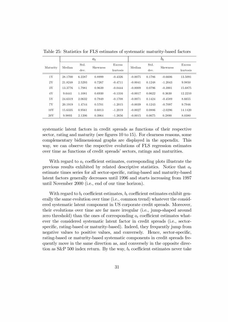
Table 25: Statistics for FLS estimates of systematic maturity-based factors
at bt
Maturity MedianStd.
dev.Skewness
Excess
kurtosisMedian
Std.
dev.Skewness
Excess
kurtosis
1Y 28.1700 6.2287 0.8999 -0.4326 -0.0075 0.1786 -0.6606 13.5091
2Y 21.8248 2.5293 0.7267 -0.4711 -0.0041 0.1248 -1.2043 9.9850
3Y 13.3776 1.7981 0.9639 -0.0444 -0.0009 0.0796 -0.3901 15.6875
4Y 9.6441 1.1081 0.6930 -0.1316 -0.0017 0.0622 0.3630 12.2210
5Y 24.6319 2.0632 0.7949 -0.1708 -0.0071 0.1424 -0.4589 8.6655
7Y 20.1919 1.4744 0.5701 -1.2015 -0.0039 0.1243 -0.7097 9.7946
10Y 15.6335 0.9561 0.6013 -1.2019 -0.0027 0.0886 -2.0296 14.1420
20Y 9.9893 2.1206 0.3964 -1.2656 -0.0015 0.0675 0.2890 8.0380
systematic latent factors in credit spreads as functions of their respectivesector, rating and maturity (see figures 10 to 15). For clearness reasons, somecomplementary bidimensional graphs are displayed in the appendix. Thisway, we can observe the respective evolutions of FLS regression estimatesover time as functions of credit spreads’ sectors, ratings and maturities.
With regard to at coefficient estimates, corresponding plots illustrate theprevious results exhibited by related descriptive statistics. Notice that atestimate times series for all sector-specific, rating-based and maturity-basedlatent factors generally decreases until 1996 and starts increasing from 1997until November 2000 (i.e., end of our time horizon).
With regard to bt coefficient estimates, bt coefficient estimates exhibit gen-erally the same evolution over time (i.e., common trend) whatever the consid-ered systematic latent component in US corporate credit spreads. Moreover,their evolutions over time are far more irregular (i.e., jump-shaped aroundzero threshold) than the ones of corresponding at coefficient estimates what-ever the considered systematic latent factor in credit spreads (i.e., sector-specific, rating-based or maturity-based). Indeed, they frequently jump fromnegative values to positive values, and conversely. Hence, sector-specific,rating-based or maturity-based systematic components in credit spreads fre-quently move in the same direction as, and conversely in the opposite direc-tion as S&P 500 index return. By the way, bt coefficient estimates never take
31

5
10
15
20
25
3005
/31/
1991
09/3
0/19
91
01/3
1/19
92
05/2
9/19
92
09/3
0/19
92
01/2
9/19
93
05/3
1/19
93
09/3
0/19
93
01/3
1/19
94
05/3
1/19
94
09/3
0/19
94
01/3
1/19
95
05/3
1/19
95
09/2
9/19
95
01/3
1/19
96
05/3
1/19
96
09/3
0/19
96
01/3
1/19
97
05/3
0/19
97
09/3
0/19
97
01/3
0/19
98
05/2
9/19
98
09/3
0/19
98
01/2
9/19
99
05/3
1/19
99
09/3
0/19
99
01/3
1/20
00
05/3
1/20
00
09/2
9/20
00
Date
IN BF TL PWa
t
Figure 10: FLS estimates for sector-specific systematic factors05
/31/
1991
12/3
1/19
9107
/31/
1992
02/2
6/19
9309
/30/
1993
04/2
9/19
9411
/30/
1994
06/3
0/19
95
01/3
1/19
96
08/3
0/19
96
03/3
1/19
97
10/3
1/19
97
05/2
9/19
98
12/3
1/19
98
07/3
0/19
99
02/2
9/20
00
09/2
9/20
00
BAA3AA3
05101520253035404550
a t
Date
Rating
Figure 11: FLS estimates for rating-based systematic factors
32

05/3
1/19
9101
/31/
1992
09/3
0/19
92
05/3
1/19
93
01/3
1/19
94
09/3
0/19
94
05/3
1/19
95
01/3
1/19
96
09/3
0/19
96
05/3
0/19
97
01/3
0/19
98
09/3
0/19
98
05/3
1/19
99
01/3
1/20
00
09/2
9/20
00
17
051015202530354045
a t
Date
Maturity(years)
Figure 12: FLS estimates for maturity-based systematic factors
-0,9
-0,4
0,1
0,6
1,1
1,6
05/31
/1991
09/30
/1991
01/31
/1992
05/29
/1992
09/30
/1992
01/29
/1993
05/31
/1993
09/30
/1993
01/31
/1994
05/31
/1994
09/30
/1994
01/31
/1995
05/31
/1995
09/29
/1995
01/31
/1996
05/31
/1996
09/30
/1996
01/31
/1997
05/30
/1997
09/30
/1997
01/30
/1998
05/29
/1998
09/30
/1998
01/29
/1999
05/31
/1999
09/30
/1999
01/31
/2000
05/31
/2000
09/29
/2000
Date
IN BF TL PW
b t
Figure 13: FLS coefficient estimates for sector-specific systematic factors
33

05/31/199106/30/1992
07/30/199308/31/1994
09/29/1995
10/31/1996
11/28/1997
12/31/1998
01/31/2000
BAA
3 AA2
-1,5
-1
-0,5
0
0,5
1
1,5
b t
Date
Rating
Figure 14: FLS coefficient estimates for rating-based systematic factors
05/3
1/19
9102
/28/
1992
11/3
0/19
9208
/31/
1993
05/3
1/19
9402
/28/
1995
11/3
0/19
95
08/3
0/19
96
05/3
0/19
97
02/2
7/19
98
11/3
0/19
98
08/3
1/19
99
05/3
1/20
00 1 10
-1
-0,8
-0,6
-0,4
-0,2
0
0,2
0,4
0,6
0,8
1
b t
Date
Maturity (years)
Figure 15: FLS coefficient estimates for maturity-based systematic factors
34

the unit value18 whatever the considered systematic sector-specific, rating-based and maturity-based systematic components. Such a feature has a highsignificance insofar as bt coefficient estimates should be unity/constant ifS&P 500 market index were a perfect/good proxy of the systematic com-ponent (i.e., common latent component) in credit spreads as a function ofsector, rating and maturity. Therefore, S&P 500 index is a biased proxy ofthe systematic risk component in US corporate credit spreads as a functionof industry, rating and maturity. In unreported results, we computed thenon-parametric correlation coefficients (i.e., Spearman’s rho and Kendall’stau) between S&P 500 index return and both credit spreads and related sys-tematic sector-specific, rating-based and maturity-based components. Wefind that these correlation coefficients lie between -0.3000 and 0, and are allinsignificant at a five percent bilateral test level. Then, such results supportthe findings of Campbell et al. (2001) who showed that the idiosyncraticrisk component in S&P 500 index has skyrocketed during the 90’. Conse-quently, S&P 500 index is not diversified enough to represent appropriatelythe US financial market (i.e., market risk) at least over our studied time hori-zon. Such an issue makes it difficult to capture the systematic componentin credit spreads as a function of sector, rating and maturity while employ-ing S&P 500 index as a market proxy. This puzzle is of high significanceinsofar as the chosen market proxy impacts the accuracy and quality of riskquantification when distinguishing between the systematic part (i.e., marketinfluence) and the idiosyncratic (i.e., unsystematic) part of credit risk (e.g.,bidimensional Value-at-Risk quantification tool).
To bypass such a puzzle, credit risk managers should focus on the dynamiclink prevailing between S&P 500 index and US corporate credit spreads inthe light of their respective industries, ratings and maturities. This way,they could extract the systematic component in credit risk, and integratethis market component into credit risk valuation processes. To get a viewof such a link, we focus on the proportions of sector-specific, rating-basedand maturity-based systematic components in credit spreads (i.e., commonlatent factors in credit spreads as functions of sector, rating and maturity),which are explained (i.e., btRt
Mt× 100) by S&P 500 index return (see tables
26 to 28).19 The proportions of explained sector-specific, rating-based and
18In unreported results, we clearly notice that bt time series only crosses up or down theunit threshold value.19Notice that the standard deviation of explained systematic sector-specific, rating-
35

Table 26: Proportions of explained systematic sector-based factors in percent
IN BF TL PWMedian 27.1192 16.7924 20.4539 14.6739
Standard deviation 15.5532 16.3837 14.4102 16.8517Skewness -0.0142 0.6289 0.7354 0.9501
Excess kurtosis -1.1518 -0.7374 0.1790 0.1098
Table 27: Proportions of explained systematic rating-based factors in percent
Rating Median Standard deviation Skewness Excess kurtosisAAA 20.5449 14.3622 0.5381 -0.4190AA2 11.8669 14.1185 1.0748 0.4434AA3 14.2405 14.7331 0.8781 0.1749A1 13.8904 14.3840 0.9331 0.2105A2 11.1569 14.5083 1.0018 0.1890A3 14.2416 13.5309 0.7464 -0.1613BAA1 16.4819 13.4592 0.4387 -0.7303BAA2 19.3530 14.0011 0.3778 -0.8968BAA3 16.7319 13.0014 0.4401 -0.8167
maturity-based systematic components in credit spreads are reported in ab-solute value.
At a sector level, the corresponding median proportion value is the lowestfor PW sector and the highest for IN sector. All proportion time series areright-skewed except for the proportion of IN sector systematic component,which is explained by S&P 500 index return. Moreover, these proportiontimes series exhibit a negative excess kurtosis for IN and BF sectors whereasthey exhibit a positive excess kurtosis for the proportions of explained TLand PW sector systematic components. At a rating level, the correspondingmedian proportion value is the lowest for A2 rating grade and the highest forAAA rating grade. All these proportion time series are right-skewed. More-over, only the proportions of explained AA2, AA3, A1 and A2 rating-basedsystematic components exhibit a negative excess kurtosis, the other rating-
based and maturity-based components in credit spreads represents the sensitivity of creditrisk (as proxied by credit spreads’ volatility) to market risk (as proxied by the standarddeviation of explained systematic credit spread factors) as a function of industry, ratingand maturity.
36

Table 28: Proportions of explained systematic maturity-based factors in per-centMaturity Median Standard deviation Skewness Excess kurtosis1Y 16.4129 13.4630 0.4299 -0.87752Y 15.3528 13.7857 0.8517 0.09203Y 13.7789 13.7416 0.9146 -0.00314Y 12.0573 15.1499 1.1787 0.75955Y 19.3014 12.6136 0.4395 -0.22577Y 17.1784 14.4299 0.8495 0.283710Y 13.4585 14.9908 0.9267 0.109820Y 15.2368 19.4691 1.2188 0.7787
based proportions exhibiting a positive excess kurtosis. At a maturity level,the corresponding median proportion value is the lowest for the four-year ma-turity and the highest for the five-year maturity. All these proportion timeseries are right-skewed. Moreover, these proportion times series exhibit gen-erally a positive excess kurtosis except for the proportions of explained one-year, three-year and five-year maturity-based systematic components (i.e.,negative excess kurtosis).
We also plot related FLS graphs to visualize the evolution over time of theproportions of sector-specific, rating-based and maturity-based systematiccomponents in credit spreads, which are explained by S&P 500 index return(see figures 16 to 18).
Whatever the considered risk level analysis, S&P 500 index fails obviouslyto capture the systematic sector-specific, rating-based and maturity-basedcomponents in corporate credit spreads. Moreover, related time series arehighly fluctuating over our time horizon. Consequently, the sensitivity ofUS corporate credit spreads to S&P 500 index is strongly fluctuating overtime and often low (see table 29 below). Moreover, the maximum propor-tions of systematic credit spread components that are explained by S&P 500index consist respectively of 63.6223%, 58.5844% and 86.3508% / 59.8807%at sector, rating and twenty-year / other-year maturity levels. Namely, theexplanatory power/performance of S&P 500 index with regard to sector-specific, rating-based and maturity-based systematic credit spread compo-nents is generally poor and specifically low (i.e., pronounced weak values) for1992/mid-1993, mid-1994/1995 and mid-1997/September 1998 time periods.
37

0,0000
10,0000
20,0000
30,0000
40,0000
50,0000
60,0000
70,0000
05/31
/1991
09/30
/1991
01/31
/1992
05/29
/1992
09/30
/1992
01/29
/1993
05/31
/1993
09/30
/1993
01/31
/1994
05/31
/1994
09/30
/1994
01/31
/1995
05/31
/1995
09/29
/1995
01/31
/1996
05/31
/1996
09/30
/1996
01/31
/1997
05/30
/1997
09/30
/1997
01/30
/1998
05/29
/1998
09/30
/1998
01/29
/1999
05/31
/1999
09/30
/1999
01/31
/2000
05/31
/2000
09/29
/2000
Date
Prop
ortio
n (%
)IN BF TL PW
Figure 16: Proportions of explained systematic sector-based factors
0,0000
10,0000
20,0000
30,0000
40,0000
50,0000
60,0000
70,0000
05/31
/1991
10/31
/1991
03/31
/1992
08/31
/1992
01/29
/1993
06/30
/1993
11/30
/1993
04/29
/1994
09/30
/1994
02/28
/1995
07/31
/1995
12/29
/1995
05/31
/1996
10/31
/1996
03/31
/1997
08/29
/1997
01/30
/1998
06/30
/1998
11/30
/1998
04/30
/1999
09/30
/1999
02/29
/2000
07/31
/2000
Date
Prop
ortio
n (%
)
BAA3
BAA2
BAA1
A3
A2
A1
AA3
AA2
AAA
Figure 17: Proportions of explained systematic rating-based factors
38

0,0000
10,0000
20,0000
30,0000
40,0000
50,0000
60,0000
70,0000
80,0000
90,0000
100,0000
05/31
/1991
10/31
/1991
03/31
/1992
08/31
/1992
01/29
/1993
06/30
/1993
11/30
/1993
04/29
/1994
09/30
/1994
02/28
/1995
07/31
/1995
12/29
/1995
05/31
/1996
10/31
/1996
03/31
/1997
08/29
/1997
01/30
/1998
06/30
/1998
11/30
/1998
04/30
/1999
09/30
/1999
02/29
/2000
07/31
/2000
Date
Prop
ortio
n (%
)
1Y
2Y
3Y
4Y
5Y
7Y
10Y
20Y
Figure 18: Proportions of explained systematic maturity-based factors
Table 29: Proportions of credit spreads explained by SP500 index in percent
Statistics∗ Sector Rating MaturityMean 7.1893 7.7041 7.8816Median 6.2649 6.5454 6.3001Minimum 0.0269 0.0124 0.0127Maximum 43.7707 46.8931 51.3896∗Average values across sector-specific, rating-based
and maturity-based credit spreads.
39

5 Conclusion
Starting from the well-documented dependency between credit risk andmarket risk, we investigated the prevailing relationship between US corpo-rate credit spreads and S&P 500 stock index. Focusing on the bivariate riskprofile of credit spreads (i.e., the bivariate structure of credit risk, namelymarket and default risk components), we analyzed the interaction and im-pact of related systematic/market and idiosyncratic/unsystematic/defaultrisk components on credit risk level in the light of three dimensions. Thecorresponding dimensions are industry-, credit rating- and maturity-basedsensitivity analyses. Specifically, we investigated the systematic and idio-syncratic credit risk components implied by US corporate credit spreads.Our aggregate credit rating levels allowed for comparison across credit rat-ing grades while investigating the common hidden information content incredit spreads as a function of credit ratings. Furthermore, we achieved atwo-stage study focusing on both the sensitivity of credit spreads to globallyunobserved macro/systematic factors (i.e., sensitivity of credit risk to busi-ness cycle, or equivalently macroeconomic/systematic shocks) and both thecoherency and usefulness of S&P 500 stock index as a proxy of systematicrisk factor for such credit spreads. This two-stage study was run in the lightof respective credit spreads’ sectors, ratings and maturities.First, we extracted the common unobserved component of default risk
(i.e., common latent factor) from observed credit spread data in the lightof three risk dimensions, namely industry, credit rating and maturity. Thiscomponent represents the interaction between credit risk and market risk(i.e., the systematic component of credit risk). Indeed, credit risk is knownto have two components, namely a market/systematic risk component andan unsystematic/default risk component. The latter component may incor-porate liquidity effects that are peculiar to debt security or eventually tothe traded asset class. We showed that credit risk sensitivity to market riskdepends on the level of the study that is achieved. Specifically, we analyzedcredit spreads’ sensitivity to the financial market or to the business cycle ac-cording to three levels: economic sector, credit rating, and finally maturity.Indeed, we found that the sensitivity of US corporate credit spreads to mar-ket risk (i.e., systematic credit spread components) depends on the industry,rating and maturity under consideration. Incidentally, related systematiccredit spread components exhibit a U-shaped evolution over our time hori-zon whatever the sensitivity analysis level (i.e., we lie essentially on a growth
40

business cycle trend). By the way, the previous three risk dimensions playa significant role for credit portfolio and credit line managers (see Wilson(1997a,b)), depending on the management style that is applied (e.g., timediversification, sector diversification, asset concentration). Most importantly,the common latent factor captures credit risk correlation, which is importantfor valuing multiname credit derivatives for example.Second, we attempted to assess the link prevailing between US credit
spreads and related S&P 500 index, which is commonly thought as a proxyof the systematic/market risk factor (i.e., market portfolio). We found neg-ative and insignificant non-parametric correlation coefficients (i.e., Spear-man’s rho and Kendall’s tau) between common latent factors (i.e., system-atic credit spread components) and S&P 500 stock index return in the lightof our basic three risk dimensions. Moreover, FLS regressions of systematicsector-specific, rating-based and maturity-based credit spread componentson S&P 500 index returns emphasized that S&P 500 stock index is not aconvenient proxy of the systematic component in credit spreads (i.e., com-mon unobserved component). Indeed, the average proportion of systematicsector-specific, rating-based and maturity-based credit spread componentsthat is explained by S&P 500 index return lies generally below forty threepercent, this average proportion falling below eight percent for that part ofsector-specific, rating-based and maturity-based credit spreads explained byS&P 500 index. Consequently, S&P 500 index fails to capture the system-atic risk factor driving corporate credit spreads in the light of their respec-tive sectors, ratings and maturities. However, FLS methodology exhibitedthe dynamic link prevailing between S&P 500 index return and systematicsector-specific, rating-based and maturity-based credit spread componentsover time. Therefore, estimating and anticipating soundly market influenceon credit risk evolution requires filtering the information content of S&P 500index return.Of course, our sensitivity analysis has a significant added value since it
yields important possible extensions and improvements for credit risk man-agement. For predictability prospects, our decomposition can be employedfirst in a value-at-risk (VaR) credit risk assessment framework (i.e., bidimen-sional VaR for credit risk). Indeed, describing/forecasting credit spreads’(i.e., credit risk) evolution should require to describe/forecast jointly the re-lated systematic/market component and unsystematic/default components(at sector, rating and maturity levels). Such a distinction should be employedin the VaR assessment process of credit risk insofar as the combination of
41

market risk level with default risk levels determines corresponding observedcredit risk levels (i.e., credit spreads) as functions of industry, credit ratingand maturity. This bivariate framework allows for distinguishing whetherwidening/tightening of credit spreads results from market risk and/or de-fault risk deterioration/improvement. Second, we employed Kalman linearmethodology as a filtering tool. However, Kalman methodology could beemployed as a forecasting tool in order to predict at least short term creditrisk while forecasting systematic credit risk components as functions of sec-tor, rating and maturity. Third, instead of considering credit spreads versusgovernment yields, it could be instructive to study credit spreads versus cor-responding swap rates in order to avoid bond-specific liquidity problems (seeLiu, Longstaff & Mandell (2002) and Cooper, Hillman & Lynch (2001)).Finally, future research can undertake a three-dimension study while distin-guishing between systematic, default-specific and liquidity-specific risk com-ponents in credit spreads always as functions of industry, credit rating andmaturity. Such an issue will yield a more detailed and sensitive analysis ofcredit risk evolution in the light of our three previous risk levels (see Odders-White & Ready (2006)).
6 Appendix
We report in this section some useful estimates, results and graphs.
6.1 Kalman estimates
We display in tables below the most relevant and significant Kalmanestimates we get while studying successively US corporate credit spreads atindustry, credit rating and maturity risk levels (see tables 30 to 32). Recallthat credit spreads are expressed in basis points and thereforeM0 (the initialvalue of the common latent component under consideration) is expressed inbasis points.20
The systematic common unobserved components (i.e., systematic sector-specific components) peculiar to BF, TL , PW sectors exhibit a non-stable
20M0 or Mt is that part of credit spreads, which results from systematic effects in thosecredit spreads in the light of their respective sector, rating and maturity.
42

Table 30: Kalman estimates for the sector analysis
IN BF TL PWM0 19.1372 32.8460 31.6207 25.7563αM 0.9987 1.0037 1.0137 1.0139Pt 7.5495×10⁻¹⁵ 0.7170 0.3430 0.2670
Table 31: Kalman estimates for the rating analysis
Rating M0 αM Pt
AAA 27.0143 1.0065 0.7913AA2 25.7708 1.0082 0.4863AA3 26.9711 1.0145 0.6840A1 30.6116 1.0106 0.6651A2 37.8950 1.0110 0.9907A3 33.4907 1.0097 0.7650BAA1 43.5918 1.0067 0.9539BAA2 31.1680 0.9985 0.1614BAA3 62.0104 0.9981 0.7894
evolution over time (i.e., related αM parameters are above unity) whereasthe one peculiar to IN sector is stable over time.21
The systematic common unobserved components peculiar to all rating grades(i.e., systematic rating-based components) exhibit generally a non-stable evo-lution over time except for BAA3 and BAA2 rating grades.
The systematic common unobserved components peculiar to all maturities(i.e., systematic maturity-based components) exhibit generally a non-stableevolution over time except for the one-year maturity case.
6.2 Systematic components in credit spreads
We investigate briefly the proportion of systematic sector, rating- andmaturity-based components in credit spreads. To get a view, we plot the
21Stability means that the common latent factor under consideration evolves and oscil-lates around some constant given level (whatever the magnitude of corresponding oscilla-tions).
43

Table 32: Kalman estimates for the maturity analysis
Maturity M0 αM Pt
1Y 56.0358 0.9990 0.54712Y 32.7506 1.0075 0.41483Y 21.5347 1.0043 0.39914Y 14.6423 1.0058 0.26755Y 34.6564 1.0092 0.58177Y 26.6230 1.0170 0.347210Y 20.4114 1.0135 0.210520Y 13.0281 1.0124 0.2314
proportions of systematic components in US corporate credit spreads as func-tions of industry, credit rating and maturity (see figures 19 to 21).
At a sector level, median and mean values of the proportion of system-atic sector-specific components in credit spreads are increasing functions ofmaturity and sectors. Namely, industrial credit spreads exhibit generallya lower proportion of systematic sector-specific component whereas powercredit spreads exhibit usually a higher proportion of systematic sector-specificcomponent.
At a rating level, median and mean values of the proportion of systematicrating-based components in credit spreads are generally increasing functionsof maturity until two-year maturity and then become decreasing functionsfrom two-year to ten/twenty-year maturities for IN, BF and PW sectors.This behavior does not apply to AAA industrial credit spreads as well as TLcredit spreads whose evolutions are far more irregular.
At a maturity level, median and mean values of the proportion of system-atic maturity-based components in credit spreads are decreasing functions ofmaturity. Namely, for given sector and maturity, median and mean valuesof the proportion of systematic maturity-based components in credit spreadsare also increasing functions of credit rating grades.
6.3 Median-related descriptive statistics
We introduce modified standard deviation, skewness and kurtosis sta-tistics that are based on a median specification. Indeed, we apply the classic
44

0,0000
10,0000
20,0000
30,0000
40,0000
50,0000
60,0000
70,0000
80,0000
IN01
YBAA
3 IN
07YB
AA3
IN03
YBAA
2 IN
02YB
AA1
IN10
YBAA
1 IN
05YA
3 IN
03YA
2 IN
01YA
1 IN
07YA
1 IN
03Y
AA3
IN02
YAA
2 IN
10Y
AA2
IN05
YAA
A BF
01Y
AA2
BF07
YAA
2 B
F03Y
AA
A TL
01YB
AA1
TL07
YBAA
1 TL
03YA
3 TL
01YA
2 TL
07YA
2 TL
03YA
1 TL
01Y
AA3
TL05
YAA
3 P
W02
YA3
P
W02
YA2
P
W01
YA1
PW
02YA
A3
PW01
YAA2
Credit spreads by sector
0,0000
10,0000
20,0000
30,0000
40,0000
50,0000
60,0000
Mean (%) Median (%) Std. Dev. (level)
Mea
n / M
edia
n Std. Dev.
Figure 19: Proportion of systematic sector-specific components in creditspreads
descriptive statistics principle except that we modify slightly the classic sta-tistics definition. Namely, we employ the time series median as a referencerather than its related arithmetic mean. Specifically, we consider the distancebetween a time series and its corresponding median value rather than its re-lated mean. For this purpose, we introduce new modified standard deviation(σMod), skewness (SkewnessMod) and kurtosis (KurtosisMod) as follows forany time series (Xt) with T observations:
σMod =
vuut 1
T
TXt=1
(Xt −Median (Xt))2 (12)
SkewnessMod =1
σ3Mod
× 1
T
TXt=1
(Xt −Median (Xt))3 (13)
KurtosisMod =1
σ4Mod
× 1
T
TXt=1
(Xt −Median (Xt))4 (14)
45

0,0000
10,0000
20,0000
30,0000
40,0000
50,0000
60,0000
70,0000
IN01
YBAA
3 IN
07YB
AA3
IN03
YBAA
2 IN
02YB
AA1
IN10
YBAA
1 TL
05YB
AA1
IN02
YA3
TL01
YA3
TL07
YA3
PW
05Y
A3
IN03
YA2
TL01
YA2
TL07
YA2
PW
05Y
A2
IN02
YA1
IN10
YA1
TL05
YA1
PW
05Y
A1
IN03
YAA
3 TL
02Y
AA3
TL07
YAA
3 PW
05YA
A3
IN02
YAA
2 IN
10Y
AA2
BF05
YAA
2 PW
05YA
A2
IN02
YAA
A IN
10YA
AA
BF0
3YA
AA
Credit spreads by rating
0,0000
5,0000
10,0000
15,0000
20,0000
25,0000
30,0000
35,0000
40,0000
45,0000
50,0000
Mean (%) Median (%) Std. Dev. (level)
Mea
n / M
edia
n
Std. Dev.
Figure 20: Proportion of systematic rating-based components in creditspreads
Table 33: Modified descriptive statistics for sector-based common latent fac-tors
IN BF TL PWσMod 131.7255 118.1325 152.2141 117.9650
SkewnessMod 3.7182 3.7250 4.3269 -1.4426ExcesskurtosisMod 24.9783 13.2727 23.9251 13.8961
ExcesskurtosisMod = KurtosisMod − 3 (15)
Such a specification focuses on the distribution gap between time series (Xt)and its related median value. Namely, we focus on the risk of deviation fromthe median value. Notice that for a Gaussian distribution, the median valuecoincides with the distribution mean. In such a setting, Gaussian skewnessand excess kurtosis should be zero for a standard distribution. Correspond-ing results are displayed for latent factors in tables 33 to 35 for our threeconsidered risk level analyses.
46

0,0000
20,0000
40,0000
60,0000
80,0000
100,0000
120,0000
IN01
YBAA
3 IN
01YA
2 IN
01YA
AA
TL01
YAA
3 P
W01
YA3
PW
01YA
A2
IN02
YA3
IN02
YAA
2 TL
02YB
AA1
TL02
YAA
3 IN
03YB
AA3
IN03
YA2
BF03
YAA
2 TL
03YA
2 TL
04Y
AA3
IN05
YA3
IN05
YAA
2 TL
05YB
AA1
TL05
YAA
3 PW
05YA
A3
IN07
YA3
IN07
YAA
2 TL
07YB
AA1
TL07
YAA
3 PW
07YA
A3
IN10
YBAA
1 IN
10YA
AA
TL10
YA3
PW
10Y
A2
Credit spreads by maturity
0,0000
5,0000
10,0000
15,0000
20,0000
25,0000
30,0000
35,0000
40,0000
45,0000
50,0000
Mean (%) Median (%) Std. Dev. (level)
Mea
n / M
edia
n Std. Dev.
Figure 21: Proportion of systematic maturity-based components in creditspreads
Table 34: Modified descriptive statistics for rating-based common latent fac-tors
Rating σMod SkewnessMod ExcesskurtosisMod
AAA 99.4038 2.0841 23.6365AA2 83.1024 -4.6217 53.8674AA3 67.9045 -3.5958 38.3355A1 104.7644 4.9804 24.4807A2 45.2868 3.6274 22.9917A3 71.2459 4.1170 18.7176BAA1 156.3789 4.9939 28.7179BAA2 88.3278 4.3576 18.8054BAA3 86.8026 4.5957 21.5383
47

Table 35: Modified descriptive statistics for maturity-based common latentfactors
Maturity σMod SkewnessMod ExcesskurtosisMod
1Y 121.6354 4.3949 34.84582Y 103.3175 4.6554 21.32633Y 143.3650 5.2795 30.79764Y 79.4652 -0.0069 15.76645Y 67.5092 4.6864 22.85817Y 61.3891 4.3525 27.396410Y 70.2736 1.5695 17.635620Y 102.1572 -2.2799 24.0076
With regard to sector analysis, the riskier22 is TL sector-specific latentfactor whereas the less risky is PW sector-specific latent factor. The skewnessis generally positive except for PW sector. With regard to rating analysis,the riskier is BAA1 rating grade-based latent factor whereas the less riskyis A2 rating grade-based latent factor . The skewness is generally positiveexcept for AA2 and AA3 rating grades. With regard to maturity analysis,the riskier is three-year maturity-based latent factor whereas the less risky isseven-year maturity-based latent factor . The skewness is generally positiveexcept for four- and twenty-year maturities.
6.4 Ultimate common latent factor
Employing Kalman methodology, we extract the ultimate common un-observed component that remains in latent factors. We process to this es-timation for each risk level analysis, namely sector, rating and maturity.Specifically, we extract the ultimate common components that result suc-cessively from sector-specific latent factors, rating-based latent factors andfinally maturity-based latent factors. Hence, we obtain three ultimate com-mon latent components at sector
¡MSector
t
¢, rating
³MRating
t
´and maturity³
MMaturityt
´levels respectively. These three ultimate common latent factors
should be approximately the same if the information set that is embedded ineach risk level analysis had the same content and significance.
22In terms of distribution risk relative to corresponding median value.
48

In unreported results, we find that all αM coefficients are above unity(i.e., instable ultimate latent factors over time), and α coefficients are gener-ally significant at a five percent test level and above unity (i.e., latent factorsmagnify global systematic shocks). The latter comment does not apply tosector analysis insofar as all α coefficients lie between zero and 0.5 and are notsignificant except for BF sector-specific latent factor. Moreover, the initialvariance level P0 of the ultimate common latent factor is generally insignifi-cant. Furthermore, the dynamic error variance Qt is insignificant for ratingand maturity risk level analyses whereas the initial value M0 of the ultimatecommon latent factor is insignificant only for maturity risk level analysis.Finally, resulting ultimate common latent components at sector, rating andmaturity levels respectively are right-skewed and exhibit a negative exceskurtosis. Their corresponding median values are very different form theircorresponding mean values except for maturity analysis. We also computedcorresponding Kendall and Spearman cross correlation coefficients betweenthese three ultimate common latent factors. We find that all the correlationcoefficients have a unit value, and are significant at a one percent bilateraltest level. Interesting related results are plotted in figures 22 and 23.Sector-specific, rating- and maturity-based ultimate common latent fac-
tors do not have the same level but exhibit the same trend over time. Thegrowth trend is more pronounced for the sector risk level analysis. However,obtained results are not meaningful and conclusive insofar as the result-ing ultimate common latent factors are no more than general trends (i.e.,straight lines, see figure 22). Especially, we get smooth curves resultingfrom a loss of sensitivity to economic facts. Using the whole informationset in corporate US credit spreads (i.e., aggregating the whole informationset across sectors, credit ratings and maturities respectively) yields a loss ofsector-specific, rating-based and maturity-based credit spread sensitivity tothe financial market and economic cycle. Indeed, we obtain pure evolutiontrends from which deviations can be of important magnitude. For forecastingprospects, such a level of aggregation seems then unuseful and makes littlesense. Moreover, we face seemingly some estimation problems insofar as wecannot stabilize the ultimate common latent factor variances Pt (see figure23) as initially assumed. Variances Pt tend to increase as we come closer tothe end of the business cycle growth trend...
49

0
20
40
60
80
100
120
140
160
180
200
05/3
1/19
91
09/3
0/19
91
01/3
1/19
92
05/2
9/19
92
09/3
0/19
92
01/2
9/19
93
05/3
1/19
93
09/3
0/19
93
01/3
1/19
94
05/3
1/19
94
09/3
0/19
94
01/3
1/19
95
05/3
1/19
95
09/2
9/19
95
01/3
1/19
96
05/3
1/19
96
09/3
0/19
96
01/3
1/19
97
05/3
0/19
97
09/3
0/19
97
01/3
0/19
98
05/2
9/19
98
09/3
0/19
98
01/2
9/19
99
05/3
1/19
99
09/3
0/19
99
01/3
1/20
00
05/3
1/20
00
09/2
9/20
00
Date
0
2
4
6
8
10
12
14
16
18
Sector Rating Maturity
Ulti
mat
e se
ctor
-spe
cific
late
nt fa
ctor
Ultim
ate rating/maturity-based latent factor
Figure 22: Ultimate common latent factors for sector, rating and maturityanalyses.
50

0
0,002
0,004
0,006
0,008
0,01
0,012
0,014
0,016
05/31
/1991
09/30
/1991
01/31
/1992
05/29
/1992
09/30
/1992
01/29
/1993
05/31
/1993
09/30
/1993
01/31
/1994
05/31
/1994
09/30
/1994
01/31
/1995
05/31
/1995
09/29
/1995
01/31
/1996
05/31
/1996
09/30
/1996
01/31
/1997
05/30
/1997
09/30
/1997
01/30
/1998
05/29
/1998
09/30
/1998
01/29
/1999
05/31
/1999
09/30
/1999
01/31
/2000
05/31
/2000
09/29
/2000
Date
0,00E+00
2,00E-04
4,00E-04
6,00E-04
8,00E-04
1,00E-03
1,20E-03
Sector Rating x 100 Maturity
Rating/M
aturity analysisSect
or a
naly
sis
Figure 23: Ultimate latent factor variance Pt for each risk level analysis.
6.5 FLS estimates
We plot the FLS estimates we get for systematic rating- and maturity-based factors in credit spreads. These graphs are in two dimensions overtime (see figures 24 to 27).
Obviously, at FLS estimate evolutions (i.e., trend of systematic creditspread components over time) are more stable than the evolutions of bt FLScoefficient estimates over time (i.e., instantaneous link of systematic creditspread components with S&P 500 index return).
51

5
10
15
20
25
30
35
40
45
50
05/31
/1991
10/31
/1991
03/31
/1992
08/31
/1992
01/29
/1993
06/30
/1993
11/30
/1993
04/29
/1994
09/30
/1994
02/28
/1995
07/31
/1995
12/29
/1995
05/31
/1996
10/31
/1996
03/31
/1997
08/29
/1997
01/30
/1998
06/30
/1998
11/30
/1998
04/30
/1999
09/30
/1999
02/29
/2000
07/31
/2000
Date
BAA3
BAA2
BAA1
A3
A2
A1
AA3
AA2
AAA
a t
Figure 24: FLS estimates for rating-based systematic factors
References
Allen, L., and A., Saunders. (2003). A Survey of Cyclical Effects in CreditRisk Measurement Models. Monetary and Economic Department, BISWork-ing Paper No 126.
Amato, J.D., and M., Luisi. (2006). Macro Factors in the Term Structure ofCredit Spreads. Monetary and Economic Department, BIS Working PaperNo 203.
Antoniou, A., Guney, Y., and K., Paudyal. (2006). The Determinants ofDebt Maturity Structure: Evidence from France, Germany and the UK.European Financial Management, 12(2): 161-94.
Aramov, D., Jostova, G., and A., Philipov. (2004). Corporate Credit RiskChanges: Common Factors and Firm-Level Fundamentals. Working Paper,Department of Finance, Robert H. Smith School of Business, University ofMaryland.
52

5
10
15
20
25
30
35
40
45
50
05/31
/1991
09/30
/1991
01/31
/1992
05/29
/1992
09/30
/1992
01/29
/1993
05/31
/1993
09/30
/1993
01/31
/1994
05/31
/1994
09/30
/1994
01/31
/1995
05/31
/1995
09/29
/1995
01/31
/1996
05/31
/1996
09/30
/1996
01/31
/1997
05/30
/1997
09/30
/1997
01/30
/1998
05/29
/1998
09/30
/1998
01/29
/1999
05/31
/1999
09/30
/1999
01/31
/2000
05/31
/2000
09/29
/2000
Date
1Y
2Y
3Y
4Y
5Y
7Y
10Y
20Y
a t
Figure 25: FLS estimates for maturity-based systematic factors
Bakshi, G., Madan, D., and F., Zhang. (2006). Investigating the Role ofSystematic and Firm-Specific Factors in Default Risk: Lessons from Empiri-cally Evaluating Credit Risk Models. Forthcoming in the Journal of Business79(5).
Baraton, X., and T., Cuillere. (2001). Modélisation des Spreads de Swap.Credit Special FocusWorking Paper, Crédit Agricole Indosuez Credit &BondResearch.
Berardi, A., and M., Trova. (2005). Credit Spreads and Default Proba-bilities in Emerging Market Bond Prices. Working Paper, SAFE Center,Department of Economics, University of Verona.
Berndt, A., Lookman, A. A., and I., Obrega. (2006). Default Risk Premiaand Asset Returns. Working Paper, Tepper School of Business, CarnegieMellon University.
Bongini, P., Laeven, L., and G., Majnoni. (2002). How Good Is the Marketat Assessing Bank Fragility? A Horse Race Between Different Indicators.Journal of Banking and Finance, 26(5): 1011-28.
53

-1,2
-0,7
-0,2
0,3
0,805
/31/
1991
09/3
0/19
9101
/31/
1992
05/2
9/19
9209
/30/
1992
01/2
9/19
9305
/31/
1993
09/3
0/19
9301
/31/
1994
05/3
1/19
9409
/30/
1994
01/3
1/19
9505
/31/
1995
09/2
9/19
9501
/31/
1996
05/3
1/19
9609
/30/
1996
01/3
1/19
9705
/30/
1997
09/3
0/19
9701
/30/
1998
05/2
9/19
9809
/30/
1998
01/2
9/19
9905
/31/
1999
09/3
0/19
9901
/31/
2000
05/3
1/20
0009
/29/
2000
Date
BAA3
BAA2
BAA1
A3
A2
A1
AA3
AA2
AAA
b t
Figure 26: FLS coefficient estimates for rating-based systematic factors
Boot, A. W. A., Milbourn, T. T., and A., Schmeits. (2006). Credit Ratingsas Coordination Mechanisms. Review of Financial Studies, 19(1): 81-118.
Brown, R. G., and P. Y. C., Hwang. (1997). Introduction to Random Signalsand Applied Kalman Filtering. Third Edition, John Wiley & Sons, Inc., NewYork.
Cipollini, A., and G., Missaglia. (2005). Business Cycle Effects on Port-folio Credit Risk: Scenario Generation through Dynamic Factor Analysis.Working Paper, Queen Mary, University of London.(129.3.20.41/eps/fin/papers/0502/0502010.pdf)
Collin-Dufresne, P., and R. S., Goldstein. (2001). Do Credit Spreads ReflectStationary Leverage Ratios? Journal of Finance, 56(5): 1929-57.
Collin-Dufresne, P., Goldstein, R. S., and J. S., Martin. (2001). The Deter-minants of Credit Spread Changes. Journal of Finance, 56(6): 2177-2207.
Cooper, N., Hillman, R., and D., Lynch. (2001). Interpreting Movements InHigh - yield Corporate Bond Market Spreads. Bank of England QuarterlyBulletin, 41(Spring): 110-120.
54

-1
-0,8
-0,6
-0,4
-0,2
0
0,2
0,4
0,6
0,8
1
05/3
1/19
91
09/3
0/19
91
01/3
1/19
92
05/2
9/19
92
09/3
0/19
92
01/2
9/19
93
05/3
1/19
93
09/3
0/19
93
01/3
1/19
94
05/3
1/19
94
09/3
0/19
94
01/3
1/19
95
05/3
1/19
95
09/2
9/19
95
01/3
1/19
96
05/3
1/19
96
09/3
0/19
96
01/3
1/19
97
05/3
0/19
97
09/3
0/19
97
01/3
0/19
98
05/2
9/19
98
09/3
0/19
98
01/2
9/19
99
05/3
1/19
99
09/3
0/19
99
01/3
1/20
00
05/3
1/20
00
09/2
9/20
00
Date
1Y
2Y
3Y
4Y
5Y
7Y
10Y
20Y
b t
Figure 27: FLS coefficient estimates for maturity-based systematic factors
Cressie, N., and C. K., Wikle. (2002). Space-Time Kalman Filter. In Ency-clopedia of Econometrics, edited by A. H. El-Shearawi & W. W. Piegorsch,4: 2045-2049.
Crouhy, M., Galai, D., and R., Mark. (1999). Credit Risk Revisited. Ed.David Shimko, Credit Risk: Models and Management, Risk Books, UK, 137-145.
Das, S. R., and P., Tufano. (1996). Pricing Credit Sensitive Debt WhenInterest Rates, Credit Ratings and Credit Spreads are Stochastic. Journal ofFinancial Engineering, 5(2): 161-98.
Delianedis, G., and R., Geske. (2001). The Components of Corporate CreditSpreads: Default, Recovery, Tax, Jumps, Liquidity and Market Factors.Working Paper No 22-01, University of California, Los Angeles.
Dichev, I. D. (1998). Is the Risk of Bankruptcy a Systematic Risk? Journalof Finance, 53(3): 1129-47.
Dionne, G., Gauthier, G., Hammami, K., Maurice, M., and J.-G., Simonato.
55

(2006). Default Risk, Default Risk Premiums, and Corporate Yield Spreads.Working Paper, HEC Montréal.
Driessen, J. (2005). Is Default Event Risk Priced in Corporate Bonds? Re-view of Financial Studies, 18(1): 165-95.
Duffee, G. R. (1998). The Relation Between Treasury Yields and CorporateBond yield Spreads. Journal of Finance, 53(6): 2225-41.
Elizalde, A. (2005). Do We Need to Worry About Credit Risk Correlation?Journal of Fixed Income, December: ????.
Elton, E. J., Gruber, M. J., Agrawal, D., and C., Mann. (2001). ExplainingThe Rate Spread on Corporate Bonds. Journal of Finance, 56(1): 247-77.
Ericsson, J., and O., Renault. (2003). Liquidity And Credit Risk. EFAAnnual Conference (Glasgow), Working Paper No 895.
Fama, E. F., and K. R., French. (1993). Common Risk Factors in theReturns on Stocks and Bonds. Journal of Financial Economics, 33(1): 3-56.
Fama, E. F., and K. R., French. (1989). Business Conditions and ExpectedReturns on Stocks and Bonds. Journal of Financial Economics, 25(1): 23-49.
Faulkender, M., and M., Petersen. (2005). Does the Source of Capital AffectCapital Structure? Working Paper, Kellogg Graduate School of Manage-ment, Northern University (Evanston, IL). Forthcoming in the Review ofFinancial Studies.
Fisher, L. (1959). Determinants of Risk Premiums on Corporate Bonds.Journal of Political Economy, 67(3): 217-37.
Frühwirth, M., Schneider, P., and L., Sögner. (2005). The Risk Microstruc-ture of Corporate Bonds: A Bayesian Analysis. Working Paper, Departmentof Corporate Finance, Vienna University of Economics and Business Admin-istration.
Gagliardini, P., and C., Gouriéroux. (2004). Stochastic Migration Modelswith Application to Corporate Risk. Working Paper, CREST.
56

Gatfaoui, H. (2006). From Fault Tree to Credit Risk Assessment: A CaseStudy. Forthcoming in the International Research Journal of Finance andEconomics.
Gatfaoui, H. (2005). How Does Systematic Risk Impact US Credit Spreads?A Copula Study. Banque & Marchés, 77(July-August): 5-16.
Gatfaoui, H. (2003). Risk Disaggregation and Credit Risk Valuation in aMerton Framework. Journal of Risk Finance, 4(3): 27-42.
Gersbach, H., and A., Lipponer. (2003). Firm Defaults and the CorrelationEffect. European Financial Management, 9(3): 361-77.
Hamerle, A., Liebig T., and H., Scheule. (2004). Forecasting Credit PortfolioRisk. Discussion Paper Series 2, Banking and Financial Supervision, No 01,Deutsche Bundesbank.
Hillegeist, S. A., Cram, D. P., Keating, E. K., and K. G., Lundstedt. (2002).Assessing the Probability of Bankruptcy. American Accounting AssociationAnnual Meeting, San Antonio.
Hui, C., Lo, C., and M. Huang. (2003) Estimation of Default Probability byThree-Factor Structural Model. Working Paper, Chinese University of HongKong.
Jakubik, P. (2006). Does Credit Risk Vary with Economic Cycles? TheCase of Finland. Working Paper, Institute of Economic Studies, CharlesUniversity, Prague.
Jarrow, R. A., Lando, D., and F., Yu. (2005). Default Risk and Diversifica-tion: Theory and Applications. Mathematical Finance, 15(1): 1-26.
Jarrow, R. A., and S. M., Turnbull. (2000). The Intersection of Market andCredit Risk. Journal of Banking and Finance, 24(1-2): 271-99.
Jarrow, R. A., and S. M., Turnbull. (1995b). Pricing Derivatives On Finan-cial Securities Subject to Credit Risk. Journal of Finance, 50(1): 53-86.
Jarrow, R. A., and S. M., Turnbull. (1995a). Drawing the Analogy. Risk,5(9): 63-70.
57

Jegadeesh, N., and S., Titman. (1993). Returns to Buying Winners andSelling Losers: Implications for Stock Market Efficiency. Journal of Finance,48(1): 65-91.
Kalaba, R., and L., Tesfatsion. (1990). Flexible Least Squares for Approxi-mately Linear Systems. IEE Transactions on Systems, Man, and Cybernet-ics, 20 (5): 978-89.
Kalaba, R., and L., Tesfatsion. (1989). Time-Varying Linear Regression viaFlexible Least Squares. Computers and Mathematics with Applications, 17(3): 1215-45.
Kalaba, R., and L., Tesfatsion. (1988). The Flexible Least Squares Approachto Time Varying Linear Regression. Journal of Economic Dynamics andControl, 12 (1): 43-48.
Kalman, R. E. (1960). A New Approach to Linear Filtering and PredictionProblems. Journal of Basic Engineering, Transactions of the ASME, SeriesD, 82(1): 34-45.
Kisgen, D. (2006). Credit Ratings and Capital Structure. Journal of Finance,61(3): 1035-72.
Kladroba, A. (2005). Flexible Least Squares Estimation of State Space Mod-els: An Alternative to Kalman-Filtering? Working Paper No 149, Universityof DUISBURG (Essen).
Koopman, S. J., and A., Lucas. (2005). Business and Default Cycles forCredit Risk. Journal of Applied Econometrics, 20(2): 311-23.
Koopman, S. J., Lucas, A., and P., Klaassen. (2005). Empirical Credit Cy-cles and Capital Buffer Formation. Journal of Banking and Finance, 29(12):3159-79.
Koopman, S. J., Lucas, A., and R. J. O., Daniels. (2005). A Non-GaussianPanel Time Series Model for Estimating and Decomposing Default Risk.Working Paper, Vrije Universiteit, Amsterdam.
Liu, J., Longstaff, F. A., and R. E., Mandell. (2002). The Market Price ofCredit Risk: An Empirical Analysis of Interest Rate Swap Spreads. NBERWorking Paper No 8990. Forthcoming in the Journal of Business.
58

Nickell, P., Perraudin, W., and S., Varotto. (2000). Stability of RatingTransitions. Journal of Banking and Finance, 24(1/2): 203-27.
Odders-White, E. R., and M. J., Ready. (2006). Credit Ratings And StockLiquidity. Review of Financial Studies, 19(1): 119-57.
Ofek, E., and M., Richardson. (2003). Dotcom Mania: The Rise and Fall ofInternet Stock Prices. Journal of Finance, 58(3): 1113-37.
Saita, L. (2006). The Puzzling Price of Corporate Default Risk. WorkingPaper, Stanford Graduate School of Business.
Shimko, D. C., Tejima, N., and D. R., Van Deventer. (1993). The Pricing ofRisky Debt When Interest Rates Are Stochastic. Journal of Fixed Income,3(September): 58-65.
Spahr, R. W., Schwebach, R. G., and M. A., Sunderman. (2002). Original-Issue Systematic and Default Risk Pricing Efficiency of Speculative-GradeBonds. Journal of Risk and Insurance, 69(4): 489-516.
Sun, D., Lin, W. T., and C.-C., Nieh. (2005). Credit Spread Decomposi-tion and Diversification: Evidences from Corporate Bond Indices. WorkingPaper, Department of Banking and Finance, Tamkang University, Taiwan.
Tasche, D. (2005). Risk Contributions in an Asymptotic Multi-factor Frame-work. Working Paper, Economic Research Center, Banking and FinancialSupervision, Deutsche Bundesbank.(Slides at www.bundesbank.de/download/vfz/konferenzen/20051118_eltville/paper_tasche.pdf)
Wilson, T. C. (1998). Portfolio Credit Risk. FRBNY Economic Policy Re-view, October: 71-82.
Wilson, T. C. (1997b). Portfolio Credit Risk (II). Risk, October: 56-61.
Wilson, T. C. (1997a). Portfolio Credit Risk (I). Risk, September: 111-17.
Xie, Y., Wu, C., and J., Shi. (2004). Do Macroeconomic Variables Matterfor the Pricing of Default Risk? Evidence from the Residual Analysis of theReduced-Form Model Pricing Errors. Working Paper, Whitman School ofManagement, Syracuse University.(www.fma.org/NewOrleans/Papers/3201827.pdf; site at www.fma.org/NewOrleans/NOProgram.htm)
59