Credit Ratings and Market Information∗

Alessio Piccolo†and Joel Shapiro‡

University of Oxford

December 2017

Abstract

How does market information affect credit ratings? How do credit ratings affect

market information? We analyze a model in which a credit rating agency’s (CRA’s)

rating is followed by a market for credit risk that provides a public signal - the price.

A more accurate rating decreases market informativeness, as it diminishes mispricing

and, hence, incentives for investor information acquisition. On the other hand, more-

informative trading increases CRA accuracy incentives by making rating inflation more

transparent. If the first effect is strong, policies that increase reputational sanctions

on CRAs decrease rating inflation, but at the same time decrease total surplus.

∗We thank Philip Bond, Jens Josephson, Jakub Kastl, Xuewen Liu, Meg Meyer, Stephen Morris, Marco

Pagano, Uday Rajan, Stefano Rossi, Günter Strobl, Sergio Vicente and seminar participants at Essex, Oxford,

Banca d’Italia, the LBS FIT workshop, the Barcelona GSE Forum in Financial Intermediation and Risk, the

Imperial College FTG conference, University of Naples Federico II, the Tilburg EBC Network Conference,

the Carnegie Mellon Economics of Credit Ratings Conference, the Catalan Economic Society Conference,

the Edinburgh Corporate Finance Conference, the Hong Kong FIRS Conference, the 13th CSEF-IGIER

Symposium on Economics and Institutions, and the 1st Workshop on Advances in Industrial Organization

for helpful comments.†Department of Economics, University of Oxford, Manor Road, Oxford OX1 3UQ UK. Email:

alessio.piccolo@merton.ox.ac.uk‡Saïd Business School, University of Oxford, Park End Street, Oxford OX1 1HP. Email:

Joel.Shapiro@sbs.ox.ac.uk

1

1 Introduction

Credit rating agencies (CRAs) assess credit risk. One way they learn about credit risk is

from a fundamental analysis of information conveyed to them by issuers. Other sources

of information abound - the bond market, the credit default swap (CDS) market, media

announcements, even equity analysis. How does this market information affect credit ratings?

How do credit ratings affect the informativeness of the market? In this paper, we analyze

the interaction between credit ratings and the market for credit risk.

In the model, a CRA receives information about the quality of an asset. It decides how

to rate this investment given that it will make more profits now from a higher rating, but

may diminish its reputation if the investment proves to be of poor quality. This rating is

released to the public, and investors may purchase the asset. A market for credit risk, which

may represent the credit default swap market or a secondary market for the asset, then

establishes a market price à la Kyle (1985): a speculator may acquire information to profit

off of noise traders, and a market maker clears the market. Lastly, the asset payoffs are

realized, leading to monetary payoffs for investors and a reputational payoff for the CRA.

The interaction between the CRA and the market price has two contrasting effects.

More-accurate ratings decrease the informativeness of market trading since they diminish

the speculator’s incentives to acquire information (by decreasing mispricing). From this

perspective, information revelation by the CRA and the speculator are strategic substitutes.

On the other hand, more-informative trading increases the CRA’s incentives to be accurate

by increasing transparency about whether the CRA inflated ratings and, thus, augmenting

the CRA’s reputational costs. The information coming from the market disciplines the CRA.

This also demonstrates that information revelation by the CRA and the speculator are also

strategic complements. This leads to a unique equilibrium.

We then examine the real effects of the interaction between ratings and market informa-

tion. We introduce a second investment whose quality is correlated with the initial asset.

The second investment will be undertaken if the information produced by the rating and the

secondary market for the initial asset convinces the investor that the investment is of suffi -

ciently high quality. The real effects in the model are, therefore, (i) the effect of the rating

on the initial asset’s origination and (ii) the effect of the rating and market information on

the second investment.

2

We find that if strong enough, the negative effect of accurate ratings on information

acquisition in the market can lead to a perverse result - policies such as reputational sanc-

tions (e.g., increased liability standards) that make ratings more accurate can reduce real

investment. From a different angle, our result that the market disciplines CRAs suggests

that policies to increase market informativeness (such as improving governance and trust in

exchanges) reap benefits beyond the market itself and spur investment. Intriguingly, this

also implies that when market informativeness is low, the CRA does not fill the informa-

tional gap, i.e., the CRA does not produce a lot of information either. Hence, a CRA fails

to produce information at the time when it is most valuable.

We demonstrate that these results are likely to hold when the speculator’s cost of in-

formation acquisition is low, i.e. for plain vanilla corporate bonds or when speculators are

concentrated and have reached economies of scale.

There is substantial evidence that more reliable market information makes ratings more

accurate (e.g. Gopolan, Gopolan, and Koharki (2017)).1 There is also an important literature

that connects information revealed through market prices to corporate investment policies

(e.g. Bakke and Whited (2010)). In this paper, we connect the dots by providing an

equilibrium analysis of different sources of investment information and their impact on real

investment decisions.

The model views CRA reputational concerns as arising from reduced future profits. Do

CRAs suffer reputational losses? In the case of the structured finance market, the market

(and the need for ratings) dried up as the crisis hit, and stock market valuations for Moody’s

fell significantly.2 One might view Standard and Poors’recent settlement with the U.S. gov-

ernment and states for $1.5 billion as a reputational sanction.3 In addition, a regulatory

environment that is more or less friendly to the CRAs may also affect the CRAs’reputa-

tional incentives. Lastly, Arthur Andersen’s implosion represents a severe punishment to a

certification intermediary in a similar line of business (auditing).

Next, we offer a summary of the related theoretical literature (Subsection 7.1 is dedicated

to a discussion of the empirical literature and implications of the model).

1We discuss the evidence in this paragraph in detail in Subsection 7.1.2Moody’s is the only stand-alone public company of the three major CRAs, and thus the only one that

has a public market price.3http://www.bloomberg.com/news/articles/2015-02-03/s-p-ends-legal-woes-with-1-5-billion-penalty-

with-u-s-states

3

Theoretical Literature

The link between ratings quality and reputation is key for our results. Mathis, McAndrews,

and Rochet (2009) examine how a CRA’s concern for its reputation affects its ratings qual-

ity. They present a dynamic model of reputation in which a monopolist CRA may mix

between lying and truth-telling to build up/exploit its reputation. Strausz (2005) is similar

in structure to Mathis et al. (2009), but examines information intermediaries in general.

Several papers have studied how a firm’s disclosure policy affects information aggregation

when there is a market composed of sophisticated investors and uninformed liquidity traders

(e.g. Verrecchia (1982), Diamond (1985), and Kim and Verrecchia (1991)). Goldstein and

Yang (2017) review this literature in depth. Gao and Liang (2013) focus on the real impacts

of this interaction. In these models, disclosure reduces gains to information acquisition by

speculators, as in our paper. However, we also examine information being produced by a

strategic rating agency and the two-way interaction between market information and the

rating agency’s information.

The interaction between market information and the rating agency’s information is a

type of feedback effect. There is a substantial literature on feedback effects of market prices,

which examines how markets guide real decisions and the feedback loop between the two

that results - see Bond, Edmans, and Goldstein (2012) for a review. Our paper examines the

feedback between two information providers and two real decisionmakers rather than between

one information provider (the market) and one real decision maker. Bond and Goldstein

(2015) look at both the real and informational feedback between government interventions

and market information. When the intervention consists of disclosing information, they

also find a crowding out effect of speculators’information acquisition. Goldstein and Yang

(forthcoming) demonstrate that making an exogenous public signal more informative may

reduce real effi ciency. This is related to our result that more accurate ratings may decrease

effi ciency overall, but in our model ratings are endogenous.

The rest of the paper is organized as follows. Section 2 describes the basic model. We

then proceed to characterize the market for credit risk and the rating process. In Section

3, we describe the equilibrium trading strategies in the market for risk, the speculator’s

information acquisition decision, and how this is affected by the CRA’s rating strategy. In

Section 4, we describe the equilibrium rating strategy and how this depends on the precision

of the speculator’s signal. This allows us to solve for the unique equilibrium and describe its

4

properties in Section 5. In Section 6 we extend the model to allow for subsequent investment

based on the information revealed by ratings and the market, and analyze the real effects

of information. Section 7 first discusses the empirical implications of the model and related

evidence. It then explores several assumptions and results from the model in greater detail.

Finally, Section 8 concludes. Detailed proofs are presented in the Appendix.

2 The Model

Our model has two distinct elements, the ratings process and the market for credit risk. We

first present them separately and then analyze the strategic interactions between them. The

market for ratings takes place first, and is followed by the market for credit risk.

2.1 The Ratings Process

The ratings process takes place at time t = 1, and consists of three types of agents: an issuer,

a monopoly credit-rating agency (CRA), and investors. All agents in the model are rational

and risk neutral.

The issuer has a risky investment project that he wishes to sell to investors. There are

two possible outcomes for a project: outcome y ∈ {S, F}, where S (F ) represents Success(Failure). The project returns 1 in case of success and 0 in case of failure, and the cost

of the project is I. The quality of the project is denoted by θ ∈ {B,G}, where B(G)stands for Bad(Good), and relates to its probability of failure: a bad project fails with

probability fB ∈ (0, 1), and a good project fails with probability fG ∈ (0, fB). Good and

bad investments have ex-ante probability 12of occurring. The investment quality is a priori

unknown, including to the issuer itself.

Let Vθ = 1 − fθ − I denote the NPV of a project of quality θ. We assume that good

projects should be financed (they have positive NPV, i.e., VG > 0) but that, without prior

knowledge on the quality of the project, no financing takes place (ex-ante NPV is negative,

i.e., 12VG + 1

2VB < 0). Therefore, the presence of a CRA can improve welfare by screening

projects for investors.

The CRA observes the quality of the project and offers the issuer a credit report m̃ ∈

5

{H,L}, where H signifies high and L signifies low.4 The issuer either pays a rating fee

and has the report publicized or refuses to purchase it. This allows for “rating shopping”

by the issuer. We assume that the rating fee is an exogenously specified fraction φ of the

project’s selling price. The outcome of the rating process, as observed by the investors, is

thus m ∈ {m̃,∅}, where m = m̃ signifies that the issuer had the credit report publicized by

the CRA and m = ∅ signifies that there is no rating. If the issuer refuses to buy the CRA’sreport and goes on the market as unrated, that in itself is a signal to the investors.

Investors observe the rating and decide whether they wish to buy the investment project,

and if so at what price. Investors are risk-neutral and perfectly competitive, so if they

purchase the project, they do so at the expected value of the asset given their posterior

beliefs. If the investors buy the project, it is implemented; the investment outcome - i.e.

y ∈ {S, F} - then realizes at time t = 3 and is observed by all players.

2.2 The Market Price of Risk

At time t = 2, if the investment project was sold to investors and implemented, a market for

credit risk takes place. We will describe this market as the CDS market in what follows. The

same setting can be used to model the secondary market for the asset when the speculator

is endowed with some amount of the investment.5

Let pcds denote the price for a CDS contract6 and x the net volume of trades. A CDS

contract is formalized as follows: at time t = 2, the contract is signed, and the buyer of the

swap pays an amount pcds to the swap’s seller. In return, the seller agrees that in the event

of default at time t = 3, the seller will pay the buyer an amount 1.7

4The assumption that the CRA perfectly observes the project quality simplifies the exposition but doesnot affect any of the results; the results would hold if the CRA observes a noisy signal of the project quality.

5As will be seen below, it is necessary for the speculator to be able to hide her trades to make a profit.This means she must be able to take either long or short positions. The easiest way to model this in asecondary market is to endow the speculator with some of the asset. Allowing for shorting would be equallygood, of course.

6In a CDS contract, a protection buyer pays a premium to the protection seller, in exchange for apayment from the latter if a credit event (usually bankruptcy) occurs on a given reference entity withina predetermined time period. The protection buyer does not need to hold the reference entity (“naked”CDS). The amount that the protection seller has to pay in case the credit event occurs is called the notionalamount. The premium is quoted in basis points per year of the contract’s notional amount and is called theCDS spread.

7We normalize the notional amount per contract to 1 and let pcds represent the CDS spread.

6

Trading occurs among liquidity/noise traders, one speculator and a competitive market

maker, and pcds is determined in a simplified model à la Kyle (1985). We now describe the

agents in detail:

Speculator: Having observed the rating m, the speculator decides whether to acquire

information about the investment. She privately chooses the precision of her signal ι ∈ [0, 1]

at a cost c (ι). When the speculator chooses a level of precision ι, with probability ι she

learns the project quality θ and with probability 1− ι she does not learn anything about θ.We assume:

c′ ≥ 0; c′′ > 0; c (0) = c′ (0) = 0. (1)

The more she spends on ι, the more likely she learns the quality of the project. When the

speculator learns θ, she tries to use her superior information to profit from mispricing in

the market. Let xs denote her demand. We use the convention xs < 0 when she is selling

protection and xs > 0 when she is buying protection.

Noise traders: Aggregate demand from noise traders is xn ∈ {−n; +n}, with both real-izations equally likely.

Market maker: The market maker observes the trade orders - i.e., {xs, xn}, but not theidentity of the trader submitting each order.8 Having observed {xs, xn} and m, he sets aprice pcds and clears the market. We assume that he makes zero profit, which implies pcds =

Eθ (fθ | m, {xs, xn}), where the expectation takes into account equilibrium beliefs about the

CRA’s rating strategy and the speculator’s choice of precision and trading strategy.9

Let x = xs + xn denote the total order flow. The informativeness of market trading

is defined by the speculator’s choice of precision ι. The other agents in the model do not

8As in the discrete setup of Faure-Grimaud and Gromb (2000), to ensure existence of a Perfect BayesianEquilibrium we allow the market maker to observe trade orders (but not the identity of those trade orders).

9We implicitly assume (i) that the speculator on the CDS market does not participate in the initialinvestment market and (ii) the investors who purchased in the initial investment market choose not toparticipate in the CDS market. Regarding (i), this is consistent with recent empirical work that shows thatspeculative trading concentrates in the CDS market, due to its relative liquidity advantage: see Oehmke andZawadowski (2016). We discuss this further in Subsection 7.2. Regarding (ii), we show in Subsection 7.2that risk-neutral initial investors would not want to participate in the CDS market and that while risk-averseinitial investors may want to participate in the CDS market, our results still hold.

7

directly observe the speculator’s choice of ι; we denote as ιe their expectation about this

choice.

2.3 The CRA’s Reputation and Rating Strategy

The CRA can be of two different types: strategic or committed. Let τ ∈ {S, C} denote arealized type, where S (C) stands for Strategic (Committed).10 The realization of τ is theCRA’s private information. Investors’prior beliefs about τ are given by

Pr (τ = C) = q0 ∈ (0, 1) ; Pr (τ = S) = 1− q0. (2)

The probability q0 represents the CRA’s initial reputation for being a committed type. A

committed CRA is always honest in its assessment of credit risk. A strategic CRA maximizes

the weighted sum of its profits from selling the rating and its expected reputational payoff;

this captures the tension between reputational concerns and profits from selling high ratings.

The reputational payoff is assumed to be the CRA’s reputation for being a committed type.

We represent this by the CRA’s posterior probability of being a committed type q(m,x,y),

given the rating m, the realization of the CDS market x,11 and the observable realization

of the investment y. We let γ denote the weighting factor, which represents the relative

importance of reputational payoffs to time t = 1 profits. The weighting γ can be potentially

larger than one (as, for example, in Laffont and Tirole (1993)), as future payoffs may arrive

over a long time horizon.

The CRA’s private information refers to its type and the project quality. Hence, we can

denote the CRA’s overall type by a pair (τ , θ).

Rating Strategy The committed CRA always offers a high (low) rating for a good (bad)

project. The strategic CRA chooses its report m̃ to maximize a weighted sum of its current

and future payoffs. The CRA knows that offering a low rating to the issuer is equivalent to

10This follows the approach of Fulghieri, Strobl, and Xia (2014) and Mathis, McAndrews, and Rochet(2009) (who, in turn, follow the classic approach of modeling reputation of Kreps and Wilson (1984) andMilgrom and Roberts (1984)).11As we will see, it is not important for our analysis whether the investors directly observe the amount

of trades or the corresponding price in the CDS market when updating their beliefs about the CRA’s type,since these are observationally equivalent.

8

making zero profit at t = 1, since the issuer will not purchase it: this creates the possibility

of rating inflation. Let ε be the probability with which a strategic CRA chooses to inflate

the rating for a bad project - i.e., offers a high rating after having observed a bad project.

The CRA can also under-report the signal, offering a low rating after having observed a good

project. This could allow it to build up reputation by appearing to be tough to investors.

Let δ be the probability with which a strategic CRA chooses to deflate the rating for a good

project. The rating strategy is characterized by the following probabilities:

Pr (m̃ = H | θ = G) = 1− δ; Pr (m̃ = H | θ = B) = ε. (3)

Let εe and δe denote the investors’conjectures about ε and δ, respectively.

A committed CRA is restricted to truthful ratings, whereas a strategic CRA may lie

and offer a high (low) rating to a bad (good) asset. Therefore, the issuance of a rating is

informative about the CRA’s type. The investors update their beliefs about the CRA’s type

first after the release of a rating and then, later on in the game, as more information about

the project quality becomes available (i.e., after they observe the realizations of the CDS

order flow x and asset payoff y).

Price of the Investment and the Rating Fee Let pm denote the price that investors

are willing to pay for the investment project for a given rating m. We assume that trade

occurs only if pm > 0 and, if the investors are not willing to buy the project, then pm = 0.

If the investors purchase the investment project, they do so at its expected value given their

posterior beliefs; these beliefs depend on the rating as well as the credibility of the CRA that

publicized it, which is given by the initial reputation q0 and the conjectures about rating

inflation εe and rating deflation δe.

We solve the model under the conjecture that the investors buy only when the credit

report is high. As we will see, this is consistent with the equilibrium of the game.12 13 This

12In equilibrium, the strategic CRA never deflates a good signal. This means that a low report (m̃ = L)would conclusively reveal that the investment is bad and, thus, not worth being implemented. Therefore,the issuer never publicizes a low report.13When the CRA’s initial reputation q0 is small, there always also exist babbling equilibria in which the

investors never buy the project, even when the rating is high. We discuss this further in Appendix A.1.

9

Figure 1: The timeline.

implies that the issuer chooses to publicize only a high report, and goes as unrated when the

report is low. Therefore, the investors either observe a project with a high rating (m = H)

or an unrated project (m = ∅); in the latter case they infer that the issuer was offered a lowreport which went unpurchased.

Given that the issuer buys the credit report only if it is high, the rating fee amounts to

φpH . Let qH denote the CRA’s reputation and µH the probability that the project quality

is good after a high rating is publicized; the price pH is characterized as follows:

pH = max{

0, µHVG +(1− µH

)VB}.

where

µH = Pr (θ = G | m = H) =1

1 + Pr(m=H|θ=B)Pr(m=H|θ=G)

=1

1 + (1−qH)εe

qH+(1−qH)(1−δe)

; (4)

qH = Pr (τ = C | m = H) =1

1 + 1−q0q0

Pr(m=H|τ=S)Pr(m=H|τ=C)

=1

1 + 1−q0q0

(1− δe + εe). (5)

2.4 Timing of the Model

The timing of the model is written below and summarized in Figure 1:

Time t = 0:

10

• Quality of the investment and CRA type: Nature chooses the quality of theinvestment θ ∈ {B,G} and the CRA type τ ∈ {S, C}.

Time t = 1 (Ratings Process):

• Rating and Investment Market: The CRA observes its type τ and the project

quality θ, and offers a report m̃ to the issuer.

—The issuer either pays the rating fee and has the report publicized (m = m̃) or

refuses to purchase it and goes on the market as unrated (m = ∅).

—Given the rating m, the issuer sets a price pm and tries to sell the project to

investors.

Time t = 2 (CDS Market): If the project is sold to investors and implemented, theCDS market takes place.

• Information acquisition by the speculator: The speculator chooses a level ofprecision ι and observes a signal about the project quality.

• Market orders: The noise traders and the speculator submit their orders {xs, xn}.Demand x realizes.

• Market Clearing: Having observed (m, {xs, xn}), the market maker sets a price pcds

and clears the market.

Time t = 3:

• Investment Outcome and Reputational Payoffs: The investment outcome y ∈{S, F} realizes. Having observed (m,x, y), the investors update their beliefs about the

CRA’s type.

We use Perfect Bayesian Equilibrium as the solution concept.

11

3 The CDS Market Equilibrium

We work our way backwards by first characterizing the CDS market equilibrium for given

conjectures (εe, δe) about the CRA’s rating strategy. The investors are not willing to buy the

project (and therefore the project is not implemented) when the investment goes unrated

and, thus, the CDS market does not take place in this case. Hence, we can focus on the case

where the rating is high (m = H) in what follows.

Proceeding by backward induction, we first solve for the equilibrium trading strategies

and then, given these strategies, characterize the speculator’s choice of precision.

3.1 Market Equilibrium

As in a standard Kyle-type setting, the speculator needs to camouflage her information-based

trades with noisy trading. She is, therefore, constrained to trade an amount xs ∈ {+n,−n}.14

This implies that, when the speculator is trading, the total order flow x can take only three

values - i.e., X = {−2n, 0,+2n}. If x ∈ {−n,+n}, it must be instead that the speculator isnot trading. The following Lemma characterizes the speculator’s trading strategy and the

market maker’s inference from the order flow.

Lemma 1 Given m = H and for given ιe and (εe, δe), the unique equilibrium of the CDS

market is characterized as follows:

1. The speculator chooses not to trade when she does not learn the project quality θ. When

she learns θ, her trading strategy is xs(B) = +n and xs (G) = −n;

2. The market maker infers θ = B when xs = xn = +n and x = +2n, θ = G when

xs = xn = −n and x = −2n, and nothing when x ∈ {−n, 0,+n}.

Lemma 1 is quite intuitive. The speculator buys protection when receiving negative

information about the investment, and sells otherwise. Given this trading strategy, the

market maker’s inference is also straightforward. When xs = xn = +n, both the speculator

and noise traders are buying; when xs = xn = −n, both are selling. In these first two cases,14If xs and xn were different in absolute values, the market maker could always tell them apart, and so

extract the speculator’s private information. Expected profits from these trades would then be zero for thespeculator.

12

the speculator’s private information is revealed by the trade orders, so her expected profits

from trading are zero; there is no mispricing. However, for xs = −xn (i.e., x = 0), the market

maker is unable to infer the direction of the speculator’s order, and so her private signal; the

speculator’s expected profits are positive in this case. This occurs with positive probability

and thus justifies costly information acquisition by the speculator. When x ∈ {−n,+n}, itmust be that the speculator is not trading (only noise traders are trading), and therefore x

is not informative about θ.

Notice that in equilibrium, all other agents also learn θ for any x ∈ {−2n,+2n} andnothing about the investment quality when x ∈ {−n, 0,+n}. The equilibrium price is

characterized as follows:

p̂cds (x) =

{fG if x = −2n;

fB if x = +2n.

p̂cds (x) = µHfG +(1− µH

)fB for x ∈ {−n, 0,+n} , (6)

where µH = Pr (G | m = H) as given by equation (4).

Notice that the CDS price fully reveals the market maker’s information about the project

quality θ. Therefore, it is not important for our analysis whether the investors directly

observe the total order flow x or the corresponding price in the CDS market when updating

their beliefs about the CRA’s type at time t = 3.

3.2 Informativeness of Market Trading

We need to evaluate the speculator’s expected profits in order to examine her decision on

how precise a signal to obtain. When the speculator is trading, her expected profits are zero

conditional on x ∈ {−2n,+2n} since, in this case, the trade orders reveal the speculator’sprivate information, and there is no informational advantage over the market maker. In

what follows, let p̂cds be the equilibrium price when x = 0 and let Πs denote the speculator’s

expected profits:

Πs =n

2

[µHι

(p̂cds − fG

)+(1− µH

)ι(fB − p̂cds

)]− c(ι). (7)

The ex-ante probability of observing θ = G is µHι. When observing θ = G, the speculator

13

sells protection - i.e., xs = −n. Trading profits are positive only if x = 0, which means that

xn has to be equal to +n; this occurs with probability 12. She trades n units and the expected

profit per unit is p̂cds−fG. This is because the speculator receives the premium p̂cds at t = 2,

but with probability fG the investment fails, meaning that she has to pay 1 at t = 3.

When the speculator learns θ = B, she buys protection. To make profits, she needs

xn = −n in this case, which occurs with probability 12. Her profit is fB − p̂cds, since she is

buying protection: she pays the premium p̂cds at t = 2, but at t = 3, with probability fB the

investment fails and she receives 1. This happens with ex-ante probability(1− µH

)ι.

The gross expected payoffis always non-negative for any strictly positive level of ι. Taking

the derivative of the speculator’s expected profits with respect to ι yields:

∂Πs

∂ι=n

2

[µH(p̂cds − fG

)+(1− µH

) (fB − p̂cds

)]− c′(ι). (8)

Higher precision benefits the speculator by increasing the chances that she learns the project

quality and can profit from mispricing in the market.

For a given level of expected rating inflation, the equilibrium level of precision ι̂ (εe) sets

equation (8) equal to zero. The existence and uniqueness of ι̂ (εe) ∈ [0, 1] is guaranteed by

the assumptions on the shape of the cost function. All the other agents in the model do

not directly observe the speculator’s choice of ι. However, they form consistent conjectures

about it, given common knowledge of Πs for any given level of expected rating inflation.

The effect of expected rating inflation on ι̂ (εe) depends on how ∂Πs

∂ιchanges with εe.

d

dεe

(∂Πs

∂ι

)=n

2

<0

dµH

dεe[(p̂cds − fG

)−(fB − p̂cds

)]+n

2

(2µH − 1

) >0

dp̂cds

dεe. (9)

As expected rating inflation εe increases, the rating m = H becomes a less reliable

signal for θ = G, and so it is relatively more likely that the investment is bad - i.e., µH

decreases towards the prior of 12.15 This has two different effects on ∂Πs

∂ι. On the one hand,

15In the text, we consider the case where bad and good assets are ex-ante equally likely so that, after agood rating, the investors believe that the project is more likely to be good - i.e., µH > 1

2 . This is true whenthe prior probability of the project being bad is close to 1

2 or below. This is the relevant case to examine,since here a good rating is meaningful and, therefore, inflated ratings induce investors to mistakenly purchasebad assets.

14

since the speculator earns more from trading when the project is bad,16 her incentives to

acquire information increase when εe increases; this is the first term in equation (9), which

is therefore positive. On the other hand, the market maker reacts to the rating being a less

reliable signal of quality by increasing the price. This reduces the speculator’s profits from

trade when the project is bad (the difference fB − p̂cds becomes smaller) and increases themwhen the project is good (the difference p̂cds − fG becomes larger); this is the second termin equation (9). Given that the project is more likely to be good (µH > 1

2), the increase in

expected profits dominates and this second effect is positive as well. Therefore, the marginal

benefit of precision increases with expected rating inflation.

Lemma 2 The equilibrium level of precision ι̂ (εe) is increasing in the amount of expected

rating inflation εe.

Interestingly, from the speculator’s point of view, information acquisition and rating in-

flation are strategic complements. That is, higher expected rating inflation increases the

incentive to acquire information. This occurs through the mispricing channel, as the specu-

lator can take advantage of wrong valuations due to more-opaque ratings.

4 The Rating Game

Having characterized the equilibrium trading strategies and level of precision in the CDS

market, we can now characterize the equilibrium rating strategy for a given level of expected

precision ιe. The properties of the strategic interaction between credit ratings and the market

for credit risk will then be used in the next section to characterize the unique equilibrium of

the game.

Proposition 1 For a given level of expected precision ιe, the unique equilibrium rating strat-egy is:

1. For γ ≥ 2φVGιeq0≡ γ, a strategic CRA always truthfully reports the quality of the project;

16A high rating makes the market believe the project is more likely to be good and, thus, the price p̂cds iscloser to fG than to fB , which implies that fB − p̂cds > p̂cds − fG. Hence, expected profits from trades arelarger when the speculator learns that the project is bad and buys CDS protection.

15

2. For γ < 2φVGιeq0

, a strategic CRA inflates the rating for a bad project with positive prob-

ability ε̂ (ιe) ∈ (0, 1] and never deflates the rating for a good project - i.e., δ̂ = 0.

When the strategic CRA has suffi cient reputation concerns, i.e., the weight on reputation

γ is larger than a threshold γ, it always offer honest ratings. Otherwise (γ < γ), the CRA

always inflates its ratings with positive probability.

Notice that truthful ratings depend on market monitoring to exist - the CRA must expect

ιe > 0, so that γ is finite and γ ≥ γ is feasible. This is because, when ratings are expected to

be honest, there is no reputational loss from inflating the rating for the CRA unless market

trading reveals that the project was bad (i.e., when x = +2n). 17 As we will see in Section

5, when ratings are expected to be always honest, the speculator has no incentives to acquire

information and, thus, market trading is not informative about θ. Therefore, honest ratings

are not actually possible in equilibrium and, thus, some degree of rating inflation is always

an equilibrium outcome, while rating deflation never occurs. In the rest of this section, we

analyze the building blocks that give us Proposition 1.

4.1 Equilibrium Rating Inflation

We first characterize the equilibrium level of rating inflation for a given level of expected

rating deflation δe and informativeness of market trading ιe.

The choice of rating inflation is relevant only when, at t = 1, a strategic CRA observes a

bad project (type (S, B)) and decides whether to inflate or truthfully report it. Therefore,

we focus on the strategic choice of this type in what follows.

We can write the total payoffs for the CRA as follows:

ΠB = ε{φpH + γEx,y

[q(H,x,y) | B

]}+ (1− ε) γq∅. (10)

With probability 1 − ε, the rating is not inflated (m = ∅) and the rating fee is notcollected; the project is not implemented and, thus, x and y do not realize. The continuation

reputational payoff is q∅ in this case. With probability ε, the rating is inflated to m = H

17When ratings are expected to be honest, the strategic and committed types are expected to play thesame strategies. This implies that the rating (and thus asset payoffs) is not informative about the CRA’stype unless market trading reveals the the project was actually bad and, thus, that the conjecture of honestratings was inaccurate.

16

and the fee φpH is collected; the continuation reputational payoff is Ex,y[q(H,x,y) | B

]in this

case. At time t = 1, both the total order flow of the CDS market x and the investment

outcome y have not yet realized. However, the CRA knows that the project is bad and,

thus, the expectation over realizations of x and y is conditional on θ = B.

The amount of rating inflation ε is then chosen as a best response to the conjectures εe,

δe and ιe; let ε∗ (εe, δe, ιe) denote this best response.

Definition 1 Any equilibrium level of rating inflation ε̂ (δe, ιe) has to be a value of εe that

satisfies the following fixed point condition:

ε∗ (εe, δe, ιe) = εe. (11)

Taking the derivative of ΠB with respect to ε yields:

MBI ≡ dΠB

dε= φpH + γEx,y

[q(H,x,y) | B

]− γq∅. (12)

The derivative dΠB

dεrepresents the marginal benefit of rating inflation for given εe, δe and ιe.

In order to simplify equation 12, let us now describe the distribution of x conditional on

the project being bad. With probability ιe, the speculator learns the asset quality and, thus,

buys CDS protection; with probability 12her trade is revealed to the market (x = +2n). In

this case, rating inflation is unveiled, as the investors learn that the project is bad and the

CRA inflated the rating. Therefore, the CRA loses all of its reputation, i.e., qH,+2n = 0.

When the speculator does not learn θ (and so does not trade) or when her trade is not

revealed to the market, i.e., x ∈ {−n, 0,+n}, the realization of x is not informative aboutproject quality and rating inflation is not revealed. This happens with probability 1− ιe

2; in

this case, the CRA’s posterior reputation depends only on the realization of y, i.e., qH,y.

We can rewrite the expression in equation (12) as follows:

MBI = φpH + γ

(1− ιe

2

)Ey[q(H,y) | B

]− γq∅. (13)

Lemma 3 The marginal benefit of rating inflation ε is always decreasing and continuous inεe. This implies that ε̂ (δe, ιe) is unique; we have:

1. ε̂ (δe, ιe) = 0, whenever MBI < 0 at (εe = 0, δe, ιe);

17

Figure 2: Characterization of MBI and equilibrium inflation.

2. ε̂ (δe, ιe) ∈ (0, 1] otherwise.

Figure 2 depicts the possible characterizations for the equilibrium level of rating inflation.

The marginal benefit of inflation MBI is always decreasing in expected rating inflation εe.

As εe increases, investors perceive it to be more likely that a strategic CRA inflated the

rating, so reputation updating conditional on the rating m = H is more severe. On the

other hand, the rating m = ∅ becomes a stronger signal for a committed type, so forgone

reputational payoffs when the CRA actually inflates are larger. Lastly, the rating m = H is

a less reliable signal for a good investment, which reduces the price the investors are willing

to pay for the investment and, thus, the rating fee. Therefore, incentives to inflate are lower

when expected rating inflation increases.

This implies that, for any given (δe, ιe), we have a unique equilibrium level of rating

inflation: no rating inflation when inflating is a strictly dominated action (MBI < 0),

including at εe = 0; 18 or some positive level of rating inflation when inflating is a dominant

action (MBI ≥ 0) for some positive level of expected rating inflation εe.

4.2 Equilibrium Rating Deflation

We can now characterize the equilibrium level of rating deflation.

18This equilibrium is supported by the off-equilibrium beliefs that whenm = H and x = +2n, the investorsbelieve that the project is bad and that the CRA is strategic and inflated the rating.

18

The choice of rating deflation is relevant only when, at t = 1, a strategic CRA observes a

good project (type (S, G)) and decides whether to deflate the rating. The analysis proceeds

in the same way as for the equilibrium rating inflation and, therefore, is left to the Appendix.

Here, we discuss the ideas behind the result, which is described in the following Lemma.

Lemma 4 The marginal benefit of deflation is always strictly negative in equilibrium; there-fore, a strategic CRA never deflates the rating for a good project, setting δ̂ = 0.

Deflating a good signal is a strictly dominated action for type (S, G) in equilibrium. In

equilibria with no rating inflation - i.e., ε̂ (δe, ιe) = 0, there is no reputational loss from

offering a high rating to a good project, since a high rating is not interpreted as a signal for

a strategic CRA. Therefore, the CRA has no incentive to deflate a good signal. In equilibria

with positive rating inflation - i.e., ε̂ (δe, ιe) ∈ (0, 1], the marginal benefit of deflation is

essentially the opposite of the marginal benefit of rating inflation (MBI; from equation 12),

which was always non-negative in equilibrium.19

By deflating a good signal, type (S, G) gives up on the rating fee and the low reputation

payoff γEx,y[q(H,x,y) | G

]in order to get the high reputation payoff γq∅ afterwards. As we

saw earlier, by inflating a bad signal, type (S, B) gives up on the high reputation payoff γq∅

in order to pocket the fee and receive the low reputation payoffγEx,y[q(H,x,y) | B

]afterwards.

For type (S, B), the realization of market trading x can reveal that the asset was bad and,

thus, that the rating had been inflated, in which case the CRA loses all its reputation.20

Therefore, the forgone reputational payoffs - i.e., the difference q∅ − Ex,y[q(H,x,y) | θ

], are

larger for type (S, B). This implies that selling the rating is always attractive enough that

there is no incentive to deflate.

Given that the CRA never deflates the rating for a good project, an unrated asset reveals

that project quality is bad and, thus, the investors never buy the project when m = ∅. 21

When the rating is high, their willingness to pay for the project depends on the credibility

19In equilibria with positive rating inflation, we have either a corner solution where MBI is strictlypositive, or an interior solution where MBI = 0.20For type (S, G) - i.e., conditional on θ = G, the realization of market trading takes values x ∈{−2n,−n, 0,+n}. When x = −2n, the market learns θ = G, in which case qH,−2n = q0; in the othercases, x is not informative about θ and, thus, we have Ey

[q(H,y) | G

].

21When observing m = ∅, the investors infer that the issuer was offered a low report which went unpur-chased and, thus, that project quality is bad.

19

of the CRA that publicized it, i.e., the initial reputation q0 and the conjecture about rating

inflation εe.

Lemma 5 In equilibrium, the investors always buy and implement the project when therating is high (m = H).

When ratings are honest, Lemma 5 is trivial, as a high rating is a perfect signal for a

good project. In the equilibrium with positive rating inflation (i.e., when γ < γ), Lemma

5 follows from the characterization of the marginal benefit of inflation, which must be non-

negative in equilibrium. This means that the short-term gain from inflating the rating

(i.e., the rating fee φpH) is at least as large as the forgone reputational payoffs (i.e., the

difference γq∅−γEx,y[q(H,x,y) | B

]). Since a committed CRA is restricted to truthful ratings,

whereas a strategic CRA inflates its ratings with positive probability, a high rating is a

signal for a strategic type, as it is relatively more likely to come from a strategic CRA.

Therefore, reputation is updated downward following a high rating and upward when the

asset is unrated. This means that the forgone reputational payoffs are always strictly positive

in equilibrium and so is also the rating fee - i.e., φpH > 0 which implies pH > 0. Hence, a

high rating is always credible enough that the investors are willing to buy when m = H.

4.3 The Effect of Trading Informativeness on Rating Inflation

The effect of a change in the expected informativeness of market trading ιe on equilibrium

rating inflation depends on its effect on the marginal benefit of rating inflation. Taking the

derivative of MBI with respect to ιe in equation (13) yields:

dMBI

dιe= −γ

2Ey[q(H,y) | B

]< 0.

An increase in expected precision ιe makes it more likely that rating inflation is revealed

to the market through the speculator’s trading activity.

Lemma 6 Equilibrium rating inflation ε̂ (ιe) is decreasing in the expected level of informa-

tiveness ιe.

This indicates that from the point of view of the CRA, rating inflation and market

trading informativeness are strategic substitutes. That is, more-informative market trading

20

Figure 3: Rating Inflation and Trading Informativeness Equilibrium.

gives the CRA incentives to be more accurate. This arises because market transparency

from informative trading makes reputational incentives more important.

5 Equilibrium and Comparative Statics

We have found that equilibrium rating inflation ε̂ (ιe) is decreasing in the expected level of

the informativeness of market trading ιe. On the other hand, the informativeness of market

trading (choice of precision by the speculator) ι̂ (εe) is increasing in the expected rating

inflation, εe. The fact that these effects move in opposite directions implies that there is a

unique equilibrium.

Proposition 2 There exists a unique pair of rating inflation and market trading informa-tiveness (ε̂, ι̂) such that ε̂ (ιe = ι̂) = ε̂ and ι̂ (εe = ε̂) = ι̂. In equilibrium, a strategic CRA

inflates the rating for a bad project with positive probability (i.e., ε̂ > 0) and the speculator

produces information about project quality (i.e., ι̂ > 0).

Figure 3 depicts the result in Proposition 2. The equilibrium values for market infor-

mativeness and rating inflation are ι̂ (εe) ∈ [0, 1], with ι̂ (0) = 0, and ε̂ (ιe) ∈ [0, 1], with

ε̂ (0) > 0; this implies that the two functions in Figure 3 either cross (and do so only once)

at some interior level (ε̂, ι̂) ∈ (0, 1)2, or they do not cross, and we have a corner solution -

21

i.e., (ε̂ = 1, ι̂ = ι̂ (1)) or (ε̂ = ε̂ (1) , ι̂ = 1). For any parameter constellation, we can always

find γ large enough that the corner solution is ruled out.22 Interior solutions are the most

interesting for comparative statics, so we focus on this case in what follows.

Note that equilibria with honest ratings are not possible anymore when we consider the

strategic interaction between the two markets. In order to have honest ratings, we would

need some independent information production by the market (i.e., ιe > 0). However, when

ratings are honest there is no mispricing of risk and, thus, the speculator chooses not to

acquire information about the project. The CRA anticipates this and, thus, finds it always

optimal to inflate ratings with some positive probability. Therefore, the market fails to

impose enough discipline on the CRA, making rating inflation endemic to the credit rating

process.23

We now analyze the effect of varying the volume of trades by noise traders in the market

for credit risk (n) and the weight on reputational payoffs in the CRA’s objective function

(γ). We first look at their effect on the equilibrium pair (ε̂, ι̂). Then, in Section 6 we analyze

their effects on the real investment decisions guided by the information produced in the two

markets (the market for ratings and the CDS market). We find:

Lemma 7 An increase in liquidity n increases equilibrium market informativeness ι̂ and

decreases equilibrium rating inflation ε̂. An increase in the CRA’s reputation concern γ

decreases ι̂ and decreases ε̂.

The comparative statics on n are straightforward. When n increases, the speculator can

trade more and, thus, makes more profits. Therefore, she chooses a larger ι̂ (εe) for any level

of εe (̂ι (εe) rotates counter-clockwise). Note that the volume of noisy trading does not enter

the CRA’s objective function, so that a change in n affects the equilibrium only through

its direct effect on ι̂ (εe). This implies that the new equilibrium pair will feature a higher

level of precision in the CDS market and lower rating inflation. Similar comparative statics

results apply to a decrease in the cost of precision for the speculator.

22Formally, we have an interior solution for any γ > γ̃, where γ̃ is such that MBI (ιe = 1, εe = 0) = 0.23When the strategic interaction between the two markets is considered, the threshold value of γ in

Proposition 1 becomes γ = 2φVGι̂(εe=0)q0

. Given that ι̂ (εe = 0) = 0, γ goes to infinity and, thus, we always haveγ < γ in equilibrium.

22

This comparative static has an intriguing implication. When market liquidity is low (e.g.,

when there is a crisis or markets are fragmented) or the cost of precision is large (e.g., for

complex assets), the informativeness of market trading is low. However, the CRA does not

respond and act as a substitute for information production by the market, because of the

lack of monitoring. In this sense, CRAs fail to produce information precisely when it would

be most valuable.

An increase in γ moves only ε̂ (ιe), shifting it down. This is quite intuitive: the strategic

CRA inflates less because it is more concerned about future reputation.24 Thus, the new

equilibrium pair features a lower level of both rating inflation and precision. We will demon-

strate in the next section that the decrease in information from the CDS market may have

adverse real consequences that overwhelm the benefit of improved rating quality.

6 Real Effects of Information

In this section, we present an extension to the baseline model which explores the real effects

of the information produced in the economy. There is already one real effect in the model -

information produced by the CRA affects whether the investment project is undertaken. We

now add another real effect that is standard in the literature (see, e.g., Bond, Edmans, and

Goldstein (2012)). Now, after the market for risk has realized, a new investor observes the

realizations of both the rating m and the information from the CDS market x and decides

whether to invest or not in a new investment project she is endowed with. For simplicity, we

assume that the quality of this project is perfectly correlated to the quality of the one being

implemented in the first period. We also assume that the speculator’s cost of precision has

the following functional form: c (ι) = k ι2

2. 25

We begin by describing the new elements of the model, and then examine the real effects.

6.1 New Investment Stage

We introduce another period to the model. The second investment stage takes place after the

realization of the CDS market and before the initial project outcome realizes at time t = 2.5.

24Notice that this does not affect its incentives to truthfully report good signals (i.e., deflate ratings).25This simplifies the exposition but our qualitative results do not depend on the choice of the cost function;

we could have any function satisfying the conditions in Equation 1.

23

Having observed the rating m and the order flow x, a new investor decides whether to invest

in a new investment project of size χ. The new project has the same characteristics as the

initial project26 and the quality of the projects in the two periods is perfectly correlated.27

Let y1 represent the outcome of the first investment project and y2 the outcome of the second

one. If the second project is implemented, at time t = 3 its outcome realizes and is observed

by all players.

6.2 Analysis

Given that the quality of the two projects is perfectly correlated, the investors at the two

investment stages would want to take the same decision about whether to invest or not.

However, the initial investors only observe the rating m, while the investor at time t = 2.5

observes the realization of market trading x as well as the rating m before taking action.

Therefore, when m = H and x = +2n, the first investment is implemented but the second

one is not, as x reveals that the rating was inflated and the project quality is actually bad.

Hence, the new investor chooses not to invest. Figure 4 describes the sequence of possible

events and subsequent investment decisions. The characterization of the equilibrium, as it

is described in Proposition 2, does not change when we introduce the new investment stage

- we prove this in Appendix A.5.

As a measure of the real effects of information, we consider the surplus, which we denote

by S. This consists of the NPV of the projects that are implemented minus the cost of the

precision chosen by the speculator28. Since bad projects have negative NPV, surplus S is

decreasing in the amount of bad projects that are implemented and increasing in the amount

of good projects.

We can write surplus S as follows:

S=1

2(1 + χ)VG +

1

2(1− q0) ε̂

[1 + χ

(1− ι̂

2

)]VB − c (̂ι) . (14)

26As for the initial project, a bad project fails with probability fB ∈ (0, 1), and a good project fails withprobability fG < fB . Both project types return 1 in case of success and 0 in case of failure; the cost of theproject is I. Good and bad investments have an ex-ante probability 1

2 of occurring.27This is just to simplify the exposition. We could have less than perfect correlation and different NPVs

for the two projects.28As prices in the model are transfers, they do not affect welfare. Therefore, we don’t need to consider

the prices in the market for the initial investment and the CDS market or the rating fee.

24

Figure 4: Sequence of events and investment decisions.

When project quality is good (ex-ante probability 12), the projects are implemented in both

periods and their expected NPV is VG, since the rating is always high and x never conveys

bad news about project quality θ (i.e., x ∈ {−2n,−n, 0,+n}). This is the first term in

equation (14). The weight χ represents the size of the investment which is undertaken at

the second investment stage, when both m and x have been observed by the new investor.

When project quality is bad (ex-ante probability 12), the first project is implemented only

when the CRA is strategic and inflates the rating; this happens with probability (1− q0) ε̂.

When the rating is high and the first project is implemented, the market for risk takes place

and x realizes. With probability ι̂2a bad project is revealed to the market (i.e., x = +2n)

and, thus, the second project is not implemented. With probability 1− ι̂2, the realization of

x is not informative about θ and the second project is implemented.

We make two remarks about the surplus before completing the analysis. First, notice

that the surplus S is maximized when ε̂ = 0 and ι̂ = 0, i.e., when the CRA always truthfully

reports the project quality and the speculator does not spend resources in acquiring her

own signal about it. However, as we have seen earlier in the analysis, this is never an

equilibrium. Second, notice that when the size of the second project is small (χ small),

surplus is determined by the first project, and therefore only the information from the rating

is relevant for the surplus and market information has no real effect (aside from affecting

equilibrium ratings). Both information from the rating and market information are relevant

for the second project, so as its size grows, the aggregate amount of information becomes

more important.

25

We now examine how the surplus is affected by the exogenous parameters.

Proposition 3 There always exist values for the speculator’s cost parameter (k∗, k∗∗), with

k∗∗ > k∗, and the size of the second investment project χ, such that:

1. The surplus S is always increasing in the CRA’s reputational concern γ and decreasing

in market liquidity n for any k ≥ k∗∗;

2. The surplus S is always decreasing in γ for k ≤ k∗ and χ ≥ χ, and increasing in n for

k ≤ k∗.

As we pointed out earlier, an increase in n leads to higher equilibrium precision ι̂ and

lower equilibrium rating inflation ε̂. Both of these shifts increase the amount of information

produced in the market, leading to more effi cient investment decisions. However, when the

cost of precision is large (k ≥ k∗∗), the overall surplus diminishes because of the increase

in the cost of precision that is associated with a larger ι̂. As the speculator’s payoffs don’t

enter our measure of surplus (since they represent a transfer), investment in making trading

profits is wasteful in the model.

On the other hand, an increase in the CRA’s reputational concern γ decreases rating

inflation ε̂ but also decreases precision ι̂. When precision is cheap (k ≤ k∗), the speculator

adjusts her choice of ι quite sharply to changes in the level of expected mispricing - i.e.,

rating inflation. This means that ι̂ (εe) is very sensitive to εe and, thus, the decrease in ι̂ is

much larger than the decrease in ε̂ when γ increases, reducing the effi ciency of the second

investment decision substantially.29 When the size of the second project is large (χ ≥ χ),

i.e., when future investment is more important than current investment, this leads to less

effi cient investment decisions overall. When instead the cost of precision is large (k ≥ k∗∗),

ι̂ (εe) is not very sensitive to εe and, thus, ι̂ does not move much when ε̂ decreases. In this

case, surplus S increases with γ.30 Figure 5 describes the result in Proposition 3.

Proposition 3 has important implications. When the cost of speculator information ac-

quisition is small (k ≤ k∗) and the size of the second project is large (χ ≥ χ), the surplus S is

29In a previous version of this paper (Piccolo and Shapiro 2016), we write down a measure of informative-ness and demonstrate that this effect decreases the total amount of information transmitted.30When k ∈ (k∗, k∗∗), the effects of both n and γ on S are ambiguous. For some parameters of the model,

S is non-monotonic in γ, i.e., there exists a threshold γ∗ such that: S is increasing in γ for γ ≥ γ∗, anddecreasing otherwise.

26

Figure 5: Comparative statics and Proposition 3.

decreasing in γ. This means that when the CRA becomes more concerned about future rep-

utation and rating inflation decreases, the overall effi ciency of the market declines. Therefore

policies meant to discipline the CRA’s incentives, such as larger reputational sanctions (e.g.,

increases in liability or regulatory scrutiny), may be undesirable, because of their perverse

effect on the market’s incentives to acquire information and the resulting real investment

decisions.

However, when the cost of speculator information acquisition is small (k ≤ k∗), policies

that foster market liquidity - for example, improved governance and regulation of exchanges

that instills trust and attracts trade - provide indirect discipline to the CRA by improving

information production by market participants, leading to more effi cient outcomes overall.

The cost of speculator information acquisition is more likely to be small for non-complex

assets/investment projects, where information production by the market is both reactive to

the level of mispricing and not too expensive. This could be for more plain vanilla issuances,

such as corporate bonds. Alternatively, if speculators have substantial size (either through

natural growth or acquisitions) and have invested in research infrastructure, they may have

reached economies of scale in information production.

On the other hand, when the cost of speculator information acquisition is large (k ≥ k∗∗),

the market fails to produce independent information about the asset and, thus, to both

27

monitor the CRA and guide investment decisions. In this case, a planner would prefer not to

spur speculators to acquire information due to the elevated cost. Furthermore, disciplining a

CRA (e.g., by a regulator) would provide it with incentives to reveal more information about

asset quality and improve surplus S. These large costs of speculator information acquisition

may be due to the complexity of the asset, such as in the case of structured finance products

or corporates with not much of a track record. Alternatively, this may occur if the informed

trading industry consisted of small players.

Our results also have some interesting implications for the limiting case where the CDS

market or the ratings process does not exist. Ratings become more accurate when a secondary

market on the asset is introduced - for example, when CDS start being actively traded on

the asset. This is consistent with the empirical findings of Dilly and Mahlmann (2014).

On the other hand, trading in the secondary market would be more informative if there

were no ratings on the asset. Paradoxically, for some parameter configurations, effi ciency

would be larger if the market for ratings did not exist.31 This is intriguing given the current

regulatory debate on replacing ratings with market based measures (e.g. Flannery, Houston,

and Partnoy (2010)).

7 Discussion

In this section, we begin by exploring the empirical implications of our model. We conclude

by checking the robustness of the model to alternative assumptions.

7.1 Empirical Implications

This paper examines how credit ratings and market information affect each other, and the

real implications of this interaction. In this section we examine evidence surrounding testable

implications of the model.

There are three key hypotheses the model offers for testing:

1. The model demonstrates that more-informative market trading leads to more-informative

ratings. This arises due to the disciplining effect of market information. Therefore there31This is true when (i) the project has positive ex-ante NPV and, thus, the CRA is not needed to enable

the initial financing by providing some screening of the projects and (ii) the speculator’s choice of precisionis quite reactive to εe (i.e., for k small).

28

are two elements to this hypothesis - first, do CRAs respond to incentives, particularly

negative incentives? And does market information provide such an incentive?

2. The model shows that more-informative ratings lead to less-informative market trading.

As we will discuss below, while the informational role of markets is central to finance,

there are few empirical measures of how informative trading is. Nevertheless, there are

well established measures for the informativeness of ratings: how well ratings predict

realized defaults and subsequent rating downgrades are common ones. Of course, some

papers also look at whether ratings predict CDS spreads, but that would not be suitable

for this line of inquiry.

3. We show that more-informative ratings may lead to negative real effects. The negative

real effects come from subsequent issuance and/or investment decisions whose quality

is related to the initial issue. The negative effects are more likely when the costs of

information acquisition are low for speculators. The costs may represent the complexity

associated with the investment (e.g., structured finance vs. plain vanilla corporate

bonds), the degree of information asymmetry (e.g., newer firms or ventures have less

of a track record, internet firms often have low cash flows), or the fact that speculators

are small and have not achieved economies of scale.

With regards to hypothesis (1), several studies have focused on establishing a causal link

for the disciplining effect of information on ratings. Fong, Hong, Kacperczyk, and Kubik

(2014) show that ratings become less informative about defaults and future downgrades

when equity analysis provides less information. Gopolan, Gopolan, and Koharki (2017) find

that ratings of unlisted firms in India are higher, less sensitive to financial conditions, and

contain less information about subsequent defaults than ratings of listed firms. Badoer and

Demiroglu (2017) find that regulation that mandated disclosure about price and volume

information on over-the-counter transactions of corporate debt makes ratings downgrades

more sensitive to changes in credit spreads. Dilly and Mahlmann (2014) find that ratings for

firms where there are actively traded CDS are more strongly correlated with bond spreads

at issuance, are adjusted more quickly, and are better predictors of defaults.32

32They also examine whether CDS markets discipline CRAs or provide additional information for themto use. They define issues based on whether measures of conflicts of interest are either high or low. CDSbenchmarks have a larger positive impact on rating quality when measures of conflicts of interest are high.

29

With regards to hypotheses (2) and (3), to our knowledge there are no studies examining

these links and exploring causality. We therefore suggest possible approaches that could be

used to test these conclusions.

The first issue for testing both hypotheses is establishing an exogenous shock to ratings

accuracy or inflation that doesn’t affect information gathering by speculators or real invest-

ments. In the finance literature, a few such exogenous events have been studied. Kliger and

Sarig (2000) use Moody’s 1982 surprise refinement of its ratings. Almeida et al (forthcoming)

and Adelino and Ferreira (2016) use sovereign rating downgrades, which qualify as a shock

due to sovereign ceiling policies of CRAs whereby domestic corporates are restricted to have

ratings below that of the sovereign. Begley (2015) uses financial ratio thresholds used by

CRAs. Baghai and Becker (2017) use S&P’s exclusion from the CMBS business following a

significant error. Kedia et al. (2014) demonstrate that Moody’s IPO led Moody’s to rate

bonds significantly higher than Standard and Poors.

Given the exogenous measure of ratings accuracy, in order to test hypothesis (2) a measure

of informed trading or mispricing is necessary. Informed trading is diffi cult to capture.33

Mispricing is easier, as the econometrician can look for reversals in asset prices (as in Coval

and Stafford, 2007). Such corrections can be verified to be information related if they take

place around information-based events, such as earnings announcements. The mispricing

channel might also arise indirectly; credit ratings may affect analyst forecasts which affect

market prices (for this last point, see, e.g., Womack, 1996).

Lastly, real activity is easier to measure. Firm investment policies, capital structure,

and R&D investment all fall under choices that may rely on information conveyed about

other assets. Relating informativeness to investment is more diffi cult. Bakke and Whited

(2010) show that the sensitivity of investment to Q depends on price informativeness when

correcting for measurement error. Chen, Goldstein, and Jiang (2007) demonstrate that the

sensitivity of investment to price is larger when several market microstructure measures

indicate there is more private information in the market price. Durnev, Morck, and Yeung

(2004) find a strong positive correlation between firm specific variation in stock returns and

They find similar results when they compare the impact of CDS on issuer-pays ratings (i.e., S&P, Moody’s,and Fitch) to investor-pays (Egan-Jones) ratings.33Collin-Dufresne and Fos (2015) and others have recently demonstrated that a typical measure of informed

trading such as PIN (Probability of informed trading) may not perform well when strategic choices byinformed traders are a consideration.

30

firm investment policies.

7.2 Assumptions and Extensions

In this section, we discuss two assumptions from the model in more detail:

The initial investors in the asset do not participate in the CDS market: Theinvestors who purchase the investment in the initial investment market are risk neutral and

therefore would choose not to participate in the CDS market. The reason for this is that

they suffer an informational disadvantage with respect to the market maker,34 and so cannot

make profits (in expectation) from trading in this market. However, initial investors who

are risk averse might want to participate in the CDS market, in order to buy protection for

the investment they purchased. We now discuss a simple variation of the model which could

allow for this possibility and demonstrate that, while risk-averse initial investors may want

to participate in the CDS market, our results still hold.

Suppose risk averse initial investors buy an amount of protection Λ in the CDS market.35

In this case, the speculator’s trading strategy does not change with the respect to one

specified in Lemma 1. The total order flow x then takes values in X = {Λ− 2n, Λ, Λ + 2n}when the speculator learns θ and trades the asset. If x ∈ {Λ− n, Λ + n}, it must be insteadthat the speculator is not trading. The market maker infers θ = G when x = Λ− 2n, θ = B

when x = Λ + 2n, and nothing when ∈ {Λ− n, Λ, Λ + n}. The investors anticipate theyare going to buy CDS protection when purchasing the investment at time t = 1. Their

willingness to pay for the initial investment and therefore the rating fee φpH depend on ιe

in this case, as ιe moves their expectations about the equilibrium CDS price. A suffi cient

condition for the results in the model to still hold in this framework would be that their

willingness to pay for the initial investment is non-increasing in ιe.36 This is satisfied, since

as we show in Appendix A.11, the expected price of CDS protection does not change with

34The signal observed by the speculator is not known to uninformed traders at the moment they submittheir trade orders, while the market maker learns it with positive probability in equilibrium before settingp̂cds.35We could have that Λ depends on expected rating inflation - i.e., Λ = Λ (εe), to allow for example the

investors to demand more CDS protection when εe increases, making the rating m = H a less reliable signalfor a good investment. As long as the characterization of Λ (εe) is common knowledge among the agents inthe model, none of our results would change.36This is needed for Lemma 6, which proves that dMBI

dιe < 0. If pH depends on ιe, dMBIdιe will include the

expression φ∂pH

∂ιe .

31

ιe, but its variance increases as ιe increases. The increase in variance in the price of CDS

protection decreases risk averse investors’willingness to pay for the initial investment.

The speculator does not participate in the investment market: This is consistentwith recent empirical work by Oehmke and Zawadowski (2016), who show that speculative

trading concentrates in the CDS market, due to its relative liquidity advantage. If the

speculator buys only a small amount of the investment initially, that will not affect her

behavior in the CDS market. If, however, the speculator were to buy a large amount of the

investment in the initial investment market, her incentives might change. Receiving a bad

signal could make the purchase of insurance so valuable that the speculator would not want

to mask her trades. Or if we were to model a further secondary market and liquidity shocks,

the speculator with a bad signal might not want to reveal any information whatsoever, so

as not to depress the price of the investment in the further secondary market.

8 Conclusion

Credit ratings have real effects. Therefore, an understanding of their dynamics is key. In

this paper, we analyze a strategic CRA that trades off current profits and future reputation

and examine its interaction with a market for credit risk. We look at both the information

production and real effects from this interaction. More-informative ratings decrease the

quality of information in market trading, but more-informative market trading increases the

quality of ratings. It would be interesting to incorporate competition in the rating market

and dynamics in market trading to create a richer environment.

References

[1] Adelino, M., Ferreira, M., 2016. Bank ratings and lending supply: Evidence from sov-

ereign downgrades, Review of Financial Studies, 29:7, 1709-1746.

[2] Almeida, H., I. Cunha, M. Ferreira, and F. Restrepo. 2017. The real effects of credit

ratings: The sovereign ceiling channel. Journal of Finance 72:249—90.

[3] Badoer, D.C., and Demiroglu, C. 2017. The Relevance of Credit Ratings in Transparent

Bond Markets, Working Paper, Koc University.

32

[4] Baghai, R., and Becker, B. 2017. Reputations and credit ratings– evidence from com-

mercial mortgage-backed securities. Working Paper, Stockholm School of Economics.

[5] Bakke TE, Whited TM. 2010. Which firms follow the market? An analysis of corporate

investment decisions. Rev. Financ. Stud. 23(5):1941—80

[6] Begley, T. 2015. The Real Costs of Corporate Credit Ratings. Working Paper.

[7] Bond, P., Edmans A., and Goldstein I., 2012, The Real Effects of Financial Markets,

Annual Review of Financial Economics, 4, 339-360.

[8] Bond, P. and Goldstein, I. 2015, Government Intervention and Information Aggregation

by Prices, Journal of Finance, 70, 2777-2811.

[9] Chen Q, Goldstein I, Jiang W. 2007. Price informativeness and investment sensitivity

to stock price. Review of Financial Studies 20(3):619—50.

[10] Collin-Dufresne, P. and V. Fos, 2015, Do prices reveal the presence of informed trading?

Journal of Finance 70, 1555-1582.

[11] Coval, J., and E. Stafford. 2007. Asset fire sales (and purchases) in equity markets.

Journal of Financial Economics 86:479—512.

[12] Diamond, D.W., 1985. Optimal release of information by firms. Journal of Finance 40,

1071—1094.

[13] Dilly, M. & Mählmann, T., 2014. The disciplinary role of CDS markets: Evidence from

agency ratings. Working paper.

[14] Durnev A, Morck R, Yeung B. 2004. Value-enhancing capital budgeting and firm-specific

return variation. Journal of Finance 59(1):65—105.

[15] Faure-Grimaud A. and Gromb D. 2004. Public Trading and Private Incentives. Review

of Financial Studies 17, 985-1014.

[16] Flannery, M. J., J. F. Houston, and F. Partnoy. 2010. Credit default swap spreads as

viable substitutes for Credit Ratings. University of Pennsylvania Law Review, 158(7),

2085-2123.

33

[17] Fong, K. Y., Hong, H. G., Kacperczyk, M. T., Kubik, J. D., 2014. Do security analysts

discipline credit rating agencies? Working paper, University of New South Wales.

[18] Fulghieri, P., G. Strobl, and H. Xia, 2014. The Economics of Solicited and Unsolicited

Credit Ratings, Review of Financial Studies, 27:2, 484-518.

[19] Gao P. and Liang P.J. 2013. Informational feedback, adverse selection, and optimal

disclosure policy. Journal of Accounting Research. 51:1133—1158.

[20] Goldstein, I., and L. Yang. 2017. Information Disclosure in Financial Markets. Working

Paper, University of Pennsylvania.

[21] Goldstein, I., and L. Yang. Forthcoming. Good Disclosure, Bad Disclosure. Journal of

Financial Economics.

[22] Gopolan, R., Gopolan, Y. and K. Koharki., 2017. Market Information and Rating

Agency Catering. Working Paper, Washington University in St. Louis.

[23] Kedia, S., Rajgopal, S., Zhou, X., 2014. Did going public impair Moody’s credit rating?

Journal of Financial Economics 114(2), 293-315.

[24] Kim, O., Verrecchia, R.E., 1991. Market reactions to anticipated announcements. Jour-

nal of Financial Economics 30, 273—309.

[25] Kliger, D. and O. Sarig. 2000. The information value of bond ratings. Journal of Finance

55(6), 2879—2902.

[26] Kreps, D. M., and R. Wilson. 1982. Reputation and Imperfect Information, Journal of

Economic Theory, 27, 253-279.

[27] Kyle, A. 1985. “Continuous Auctions and Insider Trading.”Econometrica 53, 1315-1335.

[28] Laffont, J.-J., and J. Tirole. 1993. A Theory of Incentives in Procurement and Regula-

tion (MIT Press, Cambridge).

[29] Mathis, J., McAndrews, J., Rochet, J.C. 2009. Rating the raters: Are reputation con-

cerns powerful enough to discipline rating agencies? Journal of Monetary Economics

56:5, 657-674.

34

[30] Milgrom, P., and J. Roberts. 1982. Predation, Reputation and Entry Deterrence, Journal

of Economic Theory, 27(2), 280-312.

[31] Oehmke, M., Zawadowski, A. forthcoming. The Anatomy of the CDS Market. Review

of Financial Studies.

[32] Strausz, R. 2005. Honest Certification and the Threat of Capture. International Journal

of Industrial Organization 23:1-2, 45-62.

[33] Verrecchia, R.E. 1982. The use of mathematical models in financial accounting. Journal

of Accounting Research 20 (Suppl.) 1—42.

[34] Womack, K. 1996. Do Brokerage Analysts’Recommendations Have Investment Value?

Journal of Finance 51 : 137—67.

A Appendix

A.1 Posterior Reputation and Beliefs

In this subsection, we derive some of the probabilities that will be useful for our analysis.

All of the probability measures take into account investors’conjectures about the strategic

CRA’s rating strategy and speculator’s choice of precision - i.e., for given (εe, δe) and ιe.

The distribution of the order flow x is implied by the equilibrium of the CDS market for

a given rating m. The CRA’s posterior reputation and investors’posterior beliefs about

project quality are obtained by using Bayes’rule whenever possible.

Posterior Reputation

Let z represent a realized information set for the investors; the CRA’s posterior reputation

given z is as follows:

qz = Pr (C |z) =Pr (z| C) q0

Pr (z| C) q0 + Pr (z| S) (1− q0)

=

{(1 + 1−q0

q0

Pr(z|S)Pr(z|C)

)−1

if Pr (z| C) 6= 0;

0 otherwise..

35

A strategic CRA is concerned about its reputation at t = 3 - i.e., q(m,x,y). We have

Pr (m,x, y | τ) =∑θ∈Θ

Pr (θ) Pr (m,x, y | τ , θ)

=∑θ∈Θ

Pr (θ) Pr (x | θ) Pr (m, y | τ , θ, x) . (15)

Notice that Pr (θ) Pr (x | θ) = Pr (x) Pr (θ | x). We can thus write

Pr (m,x, y|τ) = Pr (x)∑θ∈Θ

Pr (θ | x) Pr (m, y | τ , θ, x) . (16)

Let us now focus on Pr (m, y | τ , θ, x). When conditioning on θ, the distribution of y does

not depend on the realizations of τ and x; we have:

Pr (m, y | τ , θ, x) = Pr (y | θ) Pr (m | (τ , θ)) . (17)

where (τ , θ) is the CRA overall type.

The conditioning over x in Pr (m | (τ , θ)) is no longer relevant, since x realizes after m is

chosen. Using equations from (15) to (17), we have:

Pr (m,x, y| τ) = Pr (x)∑θ∈Θ

Pr (θ | x) Pr (y | θ) Pr (m | (τ , θ)) .

Notice that Pr (x) does not depend on τ , so it cancels out when considering Pr(m,x,y|S)Pr(m,x,y|C) in

q(m,x,y).

Beliefs about project quality

Let z represent a realized information set for the investors; the posterior probability that

the asset is good given z is as follows:

µz = Pr (G|z) =Pr (z|G) 1

2

Pr (z|G) 12

+ Pr (z|B) 12

=

{(1 + Pr(z|B)

Pr(z|G)

)−1

if Pr (z|G) 6= 0;

0 otherwise..

36

Consider the investors’posterior beliefs following a high rating, i.e., µH = Pr (G | m = H).

Notice that following a high rating, investors update the CRA’s reputation to qH ; we have:

µH =

(1 +

Pr (H|B)

Pr (H|G)

)−1

(18)

=

(1 +

(1− qH

)εe

qH + (1− qH) (1− δe)

)−1

,

where

qH =

(1 +

1− q0

q0

Pr (H| S)

Pr (H| C)

)−1

(19)

=

(1 +

1− q0

q0

12εe + 1

2(1− δe)12

)−1

=

(1 +

1− q0

q0

(1 + εe − δe))−1

.

When the project is unrated, investors update the CRA’s reputation to q∅; their posterior

about project quality is:

µ∅ =

(1 +

q∅ + (1− q∅) (1− εe)(1− q∅) δe

)−1

if δe > 0, µ∅ = 0 otherwise, (20)

where

q∅ =

(1 +

1− q0

q0

Pr (∅| S)

Pr (∅| C)

)−1

(21)

=

(1 +

1− q0

q0

12

(1− εe) + 12δe

12

)−1

=

(1 +

1− q0

q0

(1− εe + δe)

)−1

.

Investors are willing to buy the project as long as its expected NPV is positive. For a

given rating m, this means:

µmVG + (1− µm)VB > 0 ⇔ µm >|VB|

|VB|+ VG. (22)

37

Notice that |VB ||VB |+VG > 1

2, since the ex-ante NPV of the project is assumed to be negative

- i.e., 12VG+ 1

2VB < 0, which implies VG < |VB|. Therefore, whenever the investors are willing

to buy the project, they believe this is more likely to be good, i.e., µm > 12.

When the CRA’s initial reputation q0 is small, expected rating inflation εe is high, and

rating deflation δe is low, the inequality in (22) does not hold for both m = H and m = ∅.This means that, when q0 is small, there always exist conjectures (ε′, δ′) such that the

investors never buy the project, and, thus, the issuer never publicizes the rating. Therefore,

the strategic CRA is indifferent between any rating strategy and, hence, is fine with choosing

the strategy (ε′, δ′): this implies that the conjecture (ε′, δ′) represents indeed an equilibrium

of the game. In the literature on Communication Games, this type of equilibrium is referred

to as a babbling equilibrium. However, since ratings play no role in this type of equilibria,

they are not of interest for our analysis.

A.2 Proof of Lemma 1

We prove Lemma 1 in two steps. First, we prove that the described strategies are the unique

possible strategies in equilibrium. Second, we verify that, given the speculator’s strategy,

the market maker’s inference is consistent with Bayes rule.

Notice that we have:

fG ≤ p̂cds (x) ≤ fB. (23)

The inequalities in (23) set bounds for p̂cds (x): it cannot be greater than fB - i.e., the

probability of failure of a bad project - and it cannot be lower than fG - i.e., the probability of

failure of a good project. When the speculator learns θ = B and for a given realization of x, if

she buys (sells) protection, expected profit from trade is fB− p̂cds (x) (p̂cds (x)−fB). By (23),this is strictly positive (negative) when x does not reveal the speculator’s private information

to the market maker, and 0 otherwise. Thus, buying protection is always a dominant strategy

when learning θ = B. When the speculator learns θ = G and for a given realization of x, if

she sells (buys) protection, expected profit from trade is p̂cds (x)− fG (fG − p̂cds (x)), which

is strictly positive (negative) when x does not reveal the speculator’s private information to

the market maker, and 0 otherwise. Hence, selling protection is always a dominant strategy

when learning θ = G. Notice that the described strategy is strictly dominant whenever the

38

market maker does not always learn θ from x, which is the case in our setting (because of

the camouflage from the noise traders).

Now, consider the case where the speculator does not learn anything about θ. In this case,

her expectation about the probability of default of the project is E (fθ | m = H). For a given

realization of x, if she buys protection, her profit from trade is E (fθ | m = H) − p̂cds (x);

this is: (i) strictly negative when x = +2n, since the market maker then sets p̂cds (+2n) =

fB > E (fθ | m = H); (ii) zero when x = 0, since the market maker then sets p̂cds (0) =

E (fθ | m = H). If she sells protection, her profit from trade is p̂cds (x) − E (fθ | m = H);

this is strictly negative when x = −2n, since the market maker then sets p̂cds (−2n) = fG <

E (fθ | m = H), and again zero when x = 0. Hence, when the speculator does not learn

anything about θ, she is always better off not trading.

Therefore, the strategies described in Lemma 1 represent an equilibrium of the game.

It is straightforward to show that any other possible market maker’s inference from the

submitted orders admit profitable deviations by the speculator. Therefore, this is also the

unique equilibrium.

When x 6= 0, the market maker’s inference trivially satisfies Bayes rule. Here, we show

that Pr (x = 0 | θ) = 12∀θ ∈ {G,B}, and so no inference about θ is possible from x = 0.

When the speculator learns θ = G, she is selling CDS protection, so xs = −n. For x tobe 0, we need to have xn = +n, which has probability 1

2. The opposite is true when she

learns θ = B. Hence, we have:

Pr (x = 0 | G) = Pr (x = 0 | B) =1

2.

Therefore, the market maker does not learn anything about θ when x = 0.

A.3 Proof of Lemma 2

We need to show that ddεe

(∂Πs

∂ι

)> 0. We have

∂Πs

∂ι=n

2

[µH(p̂cds − fG

)+(1− µH

) (fB − p̂cds

)]− c′(ι). (24)

The convexity of the cost function implies that Πs is concave in ι and, thus, that ι̂ (εe)

39

exists and is unique. Given that p̂cds = µHfG +(1− µH

)fB, we can write:

p̂cds − fG =(1− µH

)(fB − fG) ; fB − p̂cds = µH (fB − fG) .

Therefore, we have:

∂Πs

∂ι=

n

2

[µH(1− µH

)(fB − fG) +

(1− µH

)µH (fB − fG)

]− c′(ι) (25)

= nµH(1− µH

)(fB − fG)− c′(ι).

This implies that:

d

dεe

(∂Πs

∂ι

)= n (fB − fG)

dµH

dεe(1− 2µH

).

We want to prove that ddεe

(∂Πs

∂ι

)≥ 0. We have:

µH =1

1 + (1−qH)εe

qH+(1−qH)(1−δe)

, where qH =1

1 + 1−q0q0

(1− δe + εe). (26)

Note that µH is always decreasing in εe directly and indirectly through its effect on qH ,

which is decreasing in εe. Notice also that, for the project to be sold to investors and, thus,

for the CDS market to take place, we must have µH > 12. Therefore, we have dµH

dεeand(

1− 2µH)both negative and, thus, d

dεe

(∂Πs

∂ι

)> 0.

A.4 Proof of Lemma 3

In order to prove this Lemma, we need to evaluate how the terms q(H,x,y), q∅, and pH change

with εe. First, we derive the expression q(H,x,y) and show that this is decreasing in εe for any

given y and conjectures (εe, δe, ιe).

40

Let µx = Pr (G | x);37 we have:

Pr (H, x, y| S)

Pr (H, x, y| C) =

prob. (S,G)︷ ︸︸ ︷µx (1− δe) Pr (y | G) +

prob. (S,B)︷ ︸︸ ︷(1− µx) εe Pr (y | B)

µx Pr (y | G)︸ ︷︷ ︸prob. (C,G)

. (27)

Therefore, for given εe and δe, we can write q(H,x,y) as:

q(H,x,y) =

(1 +

1− q0

q0

Pr (H, x, y| S)

Pr (H, x, y| C)

)−1

.

Note that q(H,x,y) is decreasing in εe, since Pr(H,x,y|S)Pr(H,x,y|C) is increasing in ε

e.

From equation (21), the expression for q∅ is the following:

q∅ =

(1 +

1− q0

q0

(1− εe + δe)

)−1

.

Note that q∅ is, instead, increasing in εe.

Finally, the price pH is increasing in µH which, as we discussed in Appendix A.3, is

decreasing in εe; this implies that pH is decreasing in εe as well. Therefore, we have:

dMBI

dεe= φ

∂pH

∂εe<0

+ γEx,y

dq(H,x,y)

dεe<0

| B

− dq∅

dεe>0

< 0.

A.5 Proof of Lemma 4

We need to prove that deflating the rating for a good project is always a strictly dominated

action in equilibrium.

The choice of rating deflation is relevant when a strategic CRA observes a good project

(type (S, G)) and decides whether to deflate or truthfully report it. The expected payoffs

37This is the posterior probability that the investment is good, given a realized x, when the distributionof x is as it is implied by the CDS market equilibrium. We have: µ−2n = 1, µ+2n = 0, and µx = 1

2 forx ∈ {−n, 0,+n}.

41

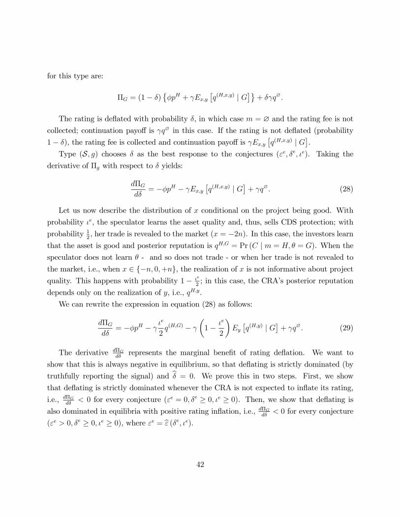
for this type are:

ΠG = (1− δ){φpH + γEx,y

[q(H,x,y) | G

]}+ δγq∅.

The rating is deflated with probability δ, in which case m = ∅ and the rating fee is notcollected; continuation payoff is γq∅ in this case. If the rating is not deflated (probability

1− δ), the rating fee is collected and continuation payoff is γEx,y[q(H,x,y) | G

].

Type (S, g) chooses δ as the best response to the conjectures (εe, δe, ιe). Taking the

derivative of Πg with respect to δ yields:

dΠG

dδ= −φpH − γEx,y

[q(H,x,y) | G

]+ γq∅. (28)

Let us now describe the distribution of x conditional on the project being good. With

probability ιe, the speculator learns the asset quality and, thus, sells CDS protection; with

probability 12, her trade is revealed to the market (x = −2n). In this case, the investors learn

that the asset is good and posterior reputation is qH,G = Pr (C | m = H, θ = G). When the

speculator does not learn θ - and so does not trade - or when her trade is not revealed to

the market, i.e., when x ∈ {−n, 0,+n}, the realization of x is not informative about projectquality. This happens with probability 1 − ιe

2; in this case, the CRA’s posterior reputation

depends only on the realization of y, i.e., qH,y.

We can rewrite the expression in equation (28) as follows:

dΠG

dδ= −φpH − γ ι

e

2q(H,G) − γ

(1− ιe

2

)Ey[q(H,y) | G

]+ γq∅. (29)

The derivative dΠG

dδrepresents the marginal benefit of rating deflation. We want to

show that this is always negative in equilibrium, so that deflating is strictly dominated (by

truthfully reporting the signal) and δ̂ = 0. We prove this in two steps. First, we show

that deflating is strictly dominated whenever the CRA is not expected to inflate its rating,

i.e., dΠG

dδ< 0 for every conjecture (εe = 0, δe ≥ 0, ιe ≥ 0). Then, we show that deflating is

also dominated in equilibria with positive rating inflation, i.e., dΠG

dδ< 0 for every conjecture

(εe > 0, δe ≥ 0, ιe ≥ 0), where εe = ε̂ (δe, ιe).

42

Step One.

When εe = 0 and δe > 0, reputation is updated downward following an unrated asset: since

the strategic type is expected to deflate but not inflate ratings, a low rating is relatively more

likely to come from a strategic type, i.e., q∅ < q0 - see equation (21). Reputation is instead

updated upward following a high rating, i.e., q(H,G) > q0 and q(H,y) > q0 for any y ∈ {S, F}.Therefore, we have:

γq∅︸︷︷︸<q0

< φpH + γιe

2q(H,G)︸ ︷︷ ︸>q0

+ γ

(1− ιe

2

)Ey[q(H,y) | G

]︸ ︷︷ ︸>q0

⇔ dΠG

dδ< 0.

When the strategic CRA is expected to always offer honest ratings (i.e., εe = δe = 0),

the rating itself is not informative about the CRA’s type, as both the strategic and the

committed type are expected to truthfully report the project quality. Therefore, we have

q(H,G) = q(H,y) = q∅ = q0 for any y ∈ {S, F}, which implies:

γq∅︸︷︷︸=q0

< φpH + γιe

2q(H,G)︸ ︷︷ ︸

=q0

+ γ

(1− ιe

2

)Ey[q(H,y) | G

]︸ ︷︷ ︸=q0

⇔ dΠG

dδ< 0.

Step Two.

From the analysis in Section 4.1, we know that in any equilibrium with positive rating

inflation we have:

dΠB

dε= φpH + γ

(1− ιe

2

)Ey[q(H,y) | B

]− γq∅ ≥ 0

⇔ φpH − γq∅ ≥ −γ(

1− ιe

2

)>0

Ey[q(H,y) | B

]>0

. (30)

In order to have positive rating deflation in equilibrium, we would need to have dΠG

dδ≥ 0.

By equation (29), this implies:

φpH − γq∅ + γιe

2q(H,G) + γ

(1− ιe

2

)Ey[q(H,y) | G

]≤ 0. (31)

The inequality in equation (30) sets a lower bound on the value of the difference φpH−γq∅.

43

In what follows, we show that the inequality in equation (31) does not hold even when the

inequality in (30) is satisfied with equality; this implies that it never holds in equilibrium.

We have:

−γ(

1− ιe

2

)Ey[q(H,y) | B

]+ γ

ιe

2q(H,G) + γ

(1− ιe

2

)Ey[q(H,y) | G

]≤ 0 (32)

⇔ γιe

2q(H,G) + γ

(1− ιe

2

){Ey[q(H,y) | G

]− Ey

[q(H,y) | B

]}≤ 0

⇔ γιe

2q(H,G)︸ ︷︷ ︸>0

+ γ

(1− ιe

2

)(fB − fG)︸ ︷︷ ︸>0, as fB>fG

(q(H,S) − q(H,F )

)≤ 0,

where the last inequality comes from the fact thatEy[q(H,y) | θ

]= fθq

(H,F )+(1− fθ) q(H,S).

Therefore, it is suffi cient to show that q(H,S) ≥ q(H,F ) for any conjectures (εe > 0, δe ≥ 0)

and, thus, the above inequality is never satisfied. We have:

q(H,S) =1

1 + 1−q0q0

(1−δe)(1−fG)+εe(1−fB)1−fG

≥ 1

1 + 1−q0q0

(1−δe)fG+εefBfG

= q(H,F )

⇔ (1− δe) fG + εefBfG

≥ (1− δe) (1− fG) + εe (1− fB)

1− fG⇔ εefB (1− fG) ≥ εe (1− fB) fG.

The inequality above is always satisfied, as we have fB > fG. Therefore, the inequality

in equation (31) is never satisfied in equilibrium and, thus, deflating the rating is always a

dominated action.

Step Two with two project outcomes.

In the proof of Lemma 3 - Appendix A.4 - we don’t use the exact characterization of y or its

distribution. This implies that Lemma 3 holds also in the setting with two project outcomes

(namely, y1 and y2) in Section 6, as the same proof applies to this setting as well - one can

simply consider y ≡ (y1, y2).

The distribution of y is used for the proof of Lemma 4. Here we show that this lemma

holds in the setting in Section 6 as well. This implies that the characterization of the equi-

librium rating strategy - as described in Proposition 1 - and, thus, of the overall equilibrium

44

of the model - Proposition 2 - does not change in the new setting.38 We omit the steps of

the proof in which the distribution of y1 and y2 is not used, as they are the same as in Step

One and Step Two above.

For Step Two, we want to show that, for any conjectures (εe > 0, δe ≥ 0, ιe ≥ 0), the

following inequality is never satisfied, so that MBD is always negative in equilibrium.

γιe

2q(H,G) + γ

(1− ιe

2

){Ey1,y2

[q(H,y1,y2) | G

]− Ey1,y2

[q(H,y1,y2) | B

]}≤ 0 (33)

We can write:

Ey1,y2[q(H,y1,y2) | G

]= fGΛ + (1− fG) Φ,

where Λ ≡ fGq(H,FF ) + (1− fG) q(H,FS); Φ ≡ fGq

(H,SF ) + (1− fG) q(H,SS).

Ey1,y2[q(H,y1,y2) | B

]= f ′BΛ′ + (1− fB) Φ′,

where Λ′ ≡ fBq(H,FF ) + (1− fB) q(H,FS); Φ′ ≡ fBq

(H,SF ) + (1− fB) q(H,SS).

Notice that we have q(H,SS) > q(H,SF ) = q(H,FS) > q(H,FF ) and fB > fG, which implies

the following: Λ > Λ′, Φ > Φ′, and Φ > Λ′. This means that:

fGΛ + (1− fG) Φ > f ′BΛ′ + (1− fB) Φ′

⇒ Ey1,y2[q(H,y1,y2) | G

]> Ey1,y2

[q(H,y1,y2) | B

].

Therefore, the inequality in equation (33) is never satisfied and, thus, deflating the rating

is always a dominated action in the setting with two project outcomes as well.

A.6 Proof of Proposition 1

Given that the strategic CRA never deflates a good signal, ratings are honest whenever the

marginal benefit of inflation is negative at the conjecture (εe = 0, δe = 0, ιe), so that inflating

38The introduction of the second investment stage does not affect the payoffs of the players in the CDSmarket and, thus, their equilibrium strategies.

45

the rating is a strictly dominated action and, thus, the conjecture εe = 0 is consistent with

the play of the game. We have:

dΠB

dε(εe, δe = 0, ιe) = φpH + γ

(1− ιe

2

)Ey[q(H,y) | B

]− γq∅

where

q∅ =q0

q0 + (1− q0) (1− εe) ; qH,y =q0

q0 + (1− q0)(

1 + Pr(y|B)Pr(y|G)

εe) .

When ratings are honest, i.e., εe = δe = 0, we have two main implications: (i) q∅ =

qH,y = q0 for any y ∈ {S, F}; 39 (ii) a high rating is a perfect signal for a good project, whichimplies pH = VG. Therefore, we can write:

dΠB

dε(εe = δe = 0) = φVG + γ

(1− ιe

2

)q0 − γq0

= φVG − γιe

2q0.

This implies:

dΠB

dε(εe = δe = 0) ≤ 0 ⇔ φVG − γ

ιe

2q0 ≤ 0

⇔ γ ≥ 2φVGιeq0

= γ.

Notice that, when γ < γ, we have MBI (εe = δe = 0, ιe) > 0. By Lemma 3, this implies

that rating inflation is positive in equilibrium when γ < γ.

A.7 Proof of Lemma 5

Here, we show that the investors always buy when m = H - i.e., pH is strictly positive in

equilibrium for every value of the initial reputation q0.

39When the strategic CRA is expected to always offer honest ratings, the rating itself is not informativeabout the CRA’s type, as both the strategic and the committed type are expected to truthfully report theproject quality.

46

In the equilibrium with honest ratings (γ ≥ γ), a high rating is a perfect signal for a

good project and, thus, investors are willing to buy a high-rated project. In this case, their

willingness to pay is the NPV of a good project, i.e., pH = VG > 0.

From the analysis in Section 4.1, we know that in any equilibrium with positive rating

inflation we must have:

φpH ≥ γq∅ − γ(

1− ιe

2

)Ey[q(H,y) | B

]. (34)

Notice that, for any given conjectures (εe > 0, δe = 0), reputation is updated upward

following m = ∅ and downward following m = H. We have:

q∅ =q0

q0 + (1− q0) (1− εe)︸ ︷︷ ︸<1

> q0;

qH,y =q0

q0 + (1− q0)

(1 +

Pr (y | B)

Pr (y | G)εe)

︸ ︷︷ ︸>1

< q0. (35)

This implies that the right-hand side of the inequality in (34) must be strictly positive.

Therefore, φpH > 0 which implies pH > 0.

A.8 Proof of Proposition 2

The first order condition for the choice of precision by the speculator (∂Πs

∂ι= 0; equation 25)

gives us the speculator’s reaction function, i.e., ι̂ (εe). We have:

∂Πs

∂ι= nµH

(1− µH

)(fB − fG)− c′(ι). (36)

When εe = 0, a high rating is interpreted as a perfect signal for a good asset (i.e., µH = 1)

and, thus, ∂Πs

∂ιis negative for any ι > 0. Therefore, the speculator chooses not to acquire

information about the project when εe = 0, i.e., ι̂ (0) = 0.

Conversely, when ιe = 0, the marginal benefit of inflation (equation 13) is always positive

at εe = 0, as the CRA can collect the fee by inflating the rating for a bad asset without

47

incurring reputational losses. Therefore, the strategic CRA always inflates with positive

probability when ιe = 0, i.e., ε̂ (0) > 0. We have:

MBI (ιe, εe) = φpH + γ

(1− ιe

2

)Ey[q(H,y) | B

]− γq∅

⇔MBI (ιe = 0, εe = 0) = φpH + γEy[q(H,y) | B

]− γq∅ = φVG > 0,

since, at εe = 0, q(H,y) = q∅ = q0 for any y and pH = VG.

Given the two remarks above, the proof for Proposition 2 is straightforward. We have

ι̂ (εe) ∈ [0, 1], with ι̂ (0) = 0, and ε̂ (ιe) ∈ [0, 1], with ε̂ (0) > 0; this implies that the two

functions in Figure 3 either do cross (and do so only once) at some interior level (ε̂, ι̂) ∈ (0, 1)2,

or they do not cross, and we have a corner solution - i.e., (ε̂ = 1, ι̂ = ι̂ (1)) or (ε̂ = ε̂ (1) , ι̂ = 1).

This means that rating inflation and market informativeness are both always strictly positive

in equilibrium.

Note that equilibria with honest ratings are not possible anymore when we consider the

strategic interaction between the two markets. When ratings are honest there is no mispricing

of risk and, thus, the speculator chooses not to acquire information about the project (i.e.,

ι̂ (0) = 0). However, inflating the rating is always a strictly dominant action when ιe = 0

and εe = 0 - i.e., MBI (ιe = 0, εe = 0) > 0. Therefore, the conjecture εe = 0 can never be

consistent with the equilibrium play of the game and we always have positive rating inflation

in equilibrium.

A.9 Proof of Lemma 7

The equilibrium pair (ε̂, ι̂) is defined by system of equations given by: (i) the first order

condition for the choice of precision by the speculator (∂Πs

∂ι= 0; equation 25); (ii) the

48

equilibrium level of rating inflation (MBI = 0; equation 13).40

nµH(1− µH

)(fB − fG)− c′ (ι) = 0 (37)

φpH + γ

(1− ι̂

2

)Ey1,y2

[q(H,y1,y2) | B

]− γq∅ = 0; (38)

where(µH , pH , q(H,y1,y2), q∅

)are functions of ε̂.

When we vary a parameter in one of the two equations, say γ in equation (38), we have

a direct effect on rating inflation dε̂dγand an indirect effect on precision dε̂

dγ∂ι̂∂ε̂.

Let us evaluate the sign of these two effects. From Lemma 2, we know that ∂ι̂∂ε̂is positive.

The left-hand side in equation (38) is the marginal benefit of inflation MBI. We can apply

the implicit function theorem to find dε̂dγ; by totally differentiating equation (38), we obtain:

∂MBI

∂γdγ +

∂MBI

∂ε̂dε̂+

∂MBI

∂ι̂

∂ι̂

∂ε̂dε̂ = 0

⇔ dε̂

dγ= −

<0∂MBI∂γ

∂MBI

∂ε̂︸ ︷︷ ︸<0

+∂MBI

∂ι̂︸ ︷︷ ︸<0

∂ι̂∂ε̂

< 0.

Therefore, both the direct effect on rating inflation and the indirect effect on precision

are negative.

The results on the comparative statics for n are similar. When we vary n in equation

(37), we have a direct effect on precision d̂ιdnand an indirect effect on rating inflation d̂ι

dn∂ε̂∂ι̂.

From Lemma 6, we know that ∂ε̂∂ι̂is negative. Let h (ε̂, n) denote the first term in equation

40As we focus on interior solutions for rating inflation, we have MBI strictly equal to zero in equilibrium.Notice also that, differently from equation (13), in the MBI below the CRA takes an expectation of bothprojects’outcome, i.e., y1 and y2. As we discussed in Appendix A.5, this does not change the characterizationof the equilibrium.

49

(37); by totally differentiating equation (37), we obtain:

∂h

∂ndn+

∂h

∂ε̂>0

∂ε̂

∂ι̂d̂ι− c′′ (ι) d̂ι = 0

⇔ d̂ι

dn=

>0∂h∂n

c′′ (ι)− ∂h

∂ε̂

∂ε̂

∂ι̂︸ ︷︷ ︸<0

> 0.

In this case, the direct effect on precision is positive and, thus, the indirect effect on

rating inflation is negative.

A.10 Proof of Proposition 3

Taking the derivative of S with respect to γ yields:

dS

dγ=dε̂

dγ

{(1− q0)

[1 + χ

(1− ι̂

2

)]VB2− χ (1− q0) ε̂

∂ι̂

∂ε̂

VB4− kι̂ ∂ι̂

∂ε̂

}.

Given that dε̂dγ< 0 from Lemma 7, dS

dγis negative when the following condition is satisfied:

∂ι̂

∂ε̂

(χ (1− q0) ε̂

|VB|4− kι̂

)≥ (1− q0)

[1 + χ

(1− ι̂

2

)]|VB|

2. (39)

The inequality in equation (39) is never satisfied when k is large: as k goes to infinity, the

term in brackets on the left-hand side becomes negative. In what follows, we show that this

inequality is instead always satisfied when k is small and χ is large.

The equilibrium level of precision is given by:

ι̂ =n

kµH(1− µH

)(fB − fG) .

Taking the derivative of ι̂ with respect to ε̂ yields:

∂ι̂

∂ε̂=n

k(fB − fG)

(1− 2µH

)<0

∂µH

∂ε̂<0

> 0.

50

Notice that ∂ι̂∂ε̂goes to infinity as k goes to zero. This is because, when precision is cheap

(k small), the speculator adjusts her choice of ι quite sharply to changes in the level of

expected mispricing - i.e., rating inflation. Conversely, when the cost of precision is large (k

large), ∂ι̂∂ε̂is small.

As χ becomes large, the inequality in equation (39) becomes:

∂ι̂

∂ε̂(1− q0) ε̂

|VB|4≥ (1− q0)

(1− ι̂

2

)|VB|

2

⇔ ∂ι̂

∂ε̂

ε̂

2≥ 1− ι̂

2.

We can rearrange the inequality above as follows:

∂ι̂

∂ε̂

ε̂

ι̂≥ 2− ι̂

ι̂. (40)

The term on the left-hand side of the inequality in equation (40) is the elasticity of the

equilibrium level of precision with respect to changes in rating inflation, i.e., the percentage

change in ι̂ = ι̂ (ε̂) in response to a one percent change in ε̂. This means that, for ε̂′ close to

ε̂ and ε̂′ > ε̂, we can rewrite the inequality in equation (40) as follows:

ι̂(ε̂′)−ι̂(ε̂)ι̂(ε̂)

ε̂′−ε̂ε̂

≥ 2− ι̂ (ε̂)

ι̂ (ε̂)

⇔ι̂(ε̂′)− ι̂ (ε̂)

2− ι̂ (ε̂)≥ ε̂′

ε̂− 1. (41)

Notice that, for ε̂′ close to ε̂, we have ι̂(ε̂′)− ι̂ (ε̂) ≈ ∂ι̂

∂ε̂

(ε̂′ − ε̂

). As we discussed earlier,

∂ι̂∂ε̂goes to infinity as k goes to zero: this implies that we can always find k close enough to

zero such that the inequality in equation (41) is satisfied.

Therefore, the inequality in equation (39) is always satisfied for k small and χ large

enough.

The results on the comparative statics for n are similar. Taking the derivative of S with

51

respect to n yields:

dS

dn=

d̂ι

dn︸︷︷︸>0

{(1− q0)

∂ε̂

∂ι̂

[1 + χ

(1− ι̂

2

)]VB2− χ (1− q0) ε̂

VB4− kι̂

}.

Hence, dSdnis positive when the following condition is satisfied:

(1− q0)∂ε̂

∂ι̂

VB2︸ ︷︷ ︸

>0

[1 + χ

(1− ι̂

2

)]≥ kι̂− χ (1− q0) ε̂

|VB|4. (42)

The right-hand side in the above inequality is always negative as k goes to zero. Therefore,

the inequality is always satisfied for k that goes to zero. Conversely, as k goes to infinity,

the right-hand side of the inequality goes to infinite as well and, thus, the inequality is never

satisfied when k is large.

A.11 Effect of ιe on expected CDS price

Given the assertion in Subsection 7.2 that initial investors don’t participate in the CDS

market, we demonstrate here that (i) the expected price of CDS protection does not depend

on ιe, but (ii) its variance increases as ιe increases. Therefore, even if the investors who

purchased the initial investment were risk averse and chose to buy CDS protection, their

willingness to pay for the initial investment would be non-increasing in ιe.

We can write the expected CDS price as:

Ex{p̂cds (x)

}= µH

ιe

2fG +

(1− µH

) ιe2fB +

(1− ιe

2

)E (fθ | m = H) , (43)

where E (fθ | m = H) = µHfG +(1− µH

)fB is the CDS price when x is not informative

about project quality, i.e., when x ∈ {−n, 0,+n}.We can rearrange equation (43) as follows:

Ex{p̂cds (x)

}=

ιe

2

[µHfG +

(1− µH

)fB]

+

(1− ιe

2

)[µHfG +

(1− µH

)fB]

= µHfG +(1− µH

)fB.

52

Notice that Ex{p̂cds (x)

}does not depend on ιe.41

Given that Ex{p̂cds (x)

}does not depend on ιe, showing that V ARx

{p̂cds (x)

}is in-

creasing in ιe is equivalent to showing that Ex{(p̂cds (x)

)2}increases with ιe. Taking the

derivative of Ex{(p̂cds (x)

)2}with respect to ιe yields:

∂Ex

{(p̂cds (x)

)2}

∂ιe=

1

2

[µHf 2

G +(1− µH

)f 2B −

(µHfG +

(1− µH

)fB)2].

We can rearrange the term in brackets in the equation above as follows:

µH(1− µH

)f 2G + µH

(1− µH

)f 2B − 2µH

(1− µH

)fBfG =

µH(1− µH

)(fG − fB)2 > 0.

Therefore,∂Ex

{(p̂cds(x))

2}

∂ιeis positive and, thus, V ARx

{p̂cds (x)

}is increasing in ιe.

41Point (i) is implied by the Law of Iterated Expectation. By the equilibrium of the CDS market, we havep̂cds (x) = Eθ (fθ | H,x); therefore:

Ex{p̂cds (x)

}= Ex {Eθ (fθ | H,x)} = Eθ (fθ | H) ,

where the last equality comes from the Law of Iterated Expectation applied on the expectation over therealization of x. This means that the expected CDS price does not depend on the realization of x, and soon its distribution - i.e., on ιe.

53