Credit Default Swaps and Debt Contracts: Spillovers and ... · Credit Default Swaps and Debt...

Finance and Economics Discussion SeriesDivisions of Research & Statistics and Monetary Affairs

Federal Reserve Board, Washington, D.C.

Credit Default Swaps and Debt Contracts: Spillovers andExtensive Default Premium Choice

R. Matthew Darst and Ehraz Refayet

2016-042

Please cite this paper as:Darst, R. Matthew and Ehraz Refayet (2016). “Credit Default Swaps and Debt Con-tracts: Spillovers and Extensive Default Premium Choice,” Finance and Economics Dis-cussion Series 2016-042. Washington: Board of Governors of the Federal Reserve System,http://dx.doi.org/10.17016/FEDS.2016.042.

NOTE: Staff working papers in the Finance and Economics Discussion Series (FEDS) are preliminarymaterials circulated to stimulate discussion and critical comment. The analysis and conclusions set forthare those of the authors and do not indicate concurrence by other members of the research staff or theBoard of Governors. References in publications to the Finance and Economics Discussion Series (other thanacknowledgement) should be cleared with the author(s) to protect the tentative character of these papers.

Credit Default Swaps and Debt Contracts:

Spillovers and Extensive Default Premium Choice∗

R. Matthew Darst† Ehraz Refayet‡

April 19, 2016

Abstract

This paper highlights two new effects of credit default swap (CDS) markets

on credit markets. First, when firms’ cash flows are correlated, CDS trading

impacts the cost of capital and investment for all firms, even those that are not

CDS obligors. Second, CDSs generate a tradeoff between default premiums

and default risk. CDSs alter firm incentives to invest along the extensive

default premium margin, even absent maturity mis-match. Firms are more

likely to issue safe debt when default premiums are high and vise versa. The

direction of the tradeoff depends on whether investors use CDSs for speculation

or hedging.

Keywords: credit derivatives, spillovers, investment, default risk.

JEL Classification: D52, D53, E44, G10, G12

∗This paper was formerly titled: “Credit Default Swaps and Firm Financing: Borrowing Costs,Spillovers, and Default Risk.” We are immensely grateful to Ana Fostel for discussions, guidance,and improvements. We also would like to thank Jay Shambaugh, Pamela Labadie, David Feldman,and Neil Ericsson for useful comments. We thank seminar participants at the 2014 NASM of theEconometric Society, 2014 Missouri Economics Conference, 2013 Georgetown Center for EconomicResearch Conference, 2013 World Finance Conference — Cyprus, 2013 ESEM-EEA joint Summermeeting, and an anonymous referee. All errors are our own. The views expressed in this paperare those of the authors and do not necessarily represent those of the Federal Reserve Board ofGovernors or anyone in the Federal Reserve System, the Department of the Treasury, or the Officeof the Comptroller of the Currency.†Federal Reserve Board of Governors: [email protected], 1801 K St. NW, Washington, D.C.

20006. (202) 628-5518.‡Office of the Comptroller of the Currency: [email protected].

1

1 Introduction

The global financial crisis of 2007-2008 underscored the need to better understand

how financial market participants price and take risk. Credit default swaps (CDSs)

are a particular type of financial instrument that market participants used with in-

creasing regularity in the build-up to the crisis. According to the Bank for Interna-

tional Settlements (BIS) the notional size of the CDS market (value of all outstanding

contracts) at its peak before the market crash in 2007 was $57 trillion. While that

number has abated mainly as a result of the multilateral netting of contracts, its size

as of the first half of 2015 was $15 trillion. Clearly the CDS market remains large

and active, and continues to engender a variety of research efforts aiming to better

understand the effects of CDS markets on capital markets.

We investigate the role of CDS trading on the cost of capital and endogenous

investment choice of multiple firms in an economy where some firms are obligors for

CDS contracts and other are not.1 We first show that the general equilibrium effects

on pricing and investment of CDS trading impact the debt contracts of all firms,

even the debt contracts for firms for whom CDS contracts do not trade. We then

show that CDS trading impacts default premiums and alters the incentives to issue

risky rather than default-risk free debt.

Building on previous work by Fostel and Geanakoplos (2012, 2016) and Che and

Sethi (2015), CDS trading affects real outcomes through its influence on investors’

marginal valuation of holding cash to as collateral to sell CDSs rather than holding

cash to buy bonds. As originally shown by Fostel and Geanakoplos (2012) and

subsequently by Che and Sethi (2015), the collateral used to back CDS contracts

re-allocates capital from the bond market to the CDS market, which changes the

demand for bonds. We use the re-allocation channel to show that in equilibrium,

when assets (firm production in our model) have correlated cash flows, an optimistic

marginal buyer prices the two assets so that the relative returns to investing in either

asset will be equal. The equivalent asset returns imply that when CDS trading alters

the demand for one type of bond, it alters the demand for the other as well. Firms

respond to changes in the cost of capital by changing their demand for investment.

1Using data from either Markit or the Depository Trust and Clearing Corporation (DTCC),there are only around 3000 firms for which a CDS contract ever exists. We do not attempt toendogenize CDS issuance in this paper; we simply take as given that the market is active only fora portion of the firms in the economy.

1

We also show that endogenous default premiums coupled with endogenous invest-

ment demand lead to interesting firm financing decisions regarding the choice to issue

debt that is default risk free rather than risky. Specifically, as the default premium

falls, the benefit of raising elevated levels of capital that cannot be repaid when cash

flow is low is reduced. As fundamentals improve firms switch to issuing fewer bonds

that can be fully repaid in all states, hence the extensive default premium choice.

We then show that for a given set of economy fundamentals, the extensive default

risk margin changes when bond buyers are permitted to trade CDSs because CDS

trading alters default premiums.

The framework in our paper is a static, general equilibrium model with two states

characterized by a commonly known aggregate productivity shock with high values in

the up state and low values in the down state. There are two firm types endowed with

different production technologies that are symmetrically impacted by the technology

shock i.e. the production technologies generate high cash flows in the up state and

low cash flows in the down state. To produce, each firm endogenously issues non-

contingent, collateralized debt. The firms know the true probability over the high and

low cash-flow states, but this is unobservable.2 We assume a portion of the cash flows

from production are not pledgeable so that production generates positive profits and

control rents. Debt financing comes from investors with heterogeneous beliefs about

the probability of the future states. We first solve the baseline model without CDS

for equilibrium bond prices, firm investment, and the states in which firms choose

to issue debt contracts characterized by positive rather than zero default premiums.

Similarly to Che and Sethi (2012), we then extend the model to incorporate CDS

contracts, where CDS purchasers must also own the underlying bond, which we call

Covered CDS Economies. This restriction on CDS ownership is then removed so

investors are free to purchase CDS without owning the underlying bond, in what we

call naked CDS economies.3

We begin by characterizing the equilibrium based on whether the debt contracts

2Alternatively, one could assume that the state probabilities reveal a non-verifiable or non-contractible signal about cash flows.

3Norden and Radoeva (2013) document that there is clear firm heterogeneity in the size of theCDS market relative to the size of the underlying bond market supporting the CDS contracts. Onenatural way to interpret the covered CDS economy is as a CDS market that is “small” relativeto the size of the underlying bond market whereby a sufficient level of investor capital remainsavailable to purchase bonds. Naked CDS economies in our framework would correspond to verylarge outstanding CDS markets relative to the underlying bond market supporting those trades.

2

issued have a positive or zero default premium. Low values of the technology shock

always result in debt contracts that contain positive risk premiums. Such debt con-

tracts allow the firm to invest as much as possible in the up state where the firm is

always the residual equity claimant. As a result of limited liability, creditors simply

take possession of firm assets in the down state. Alternatively, the capital raised for

production is limited when financed via debt contracts that are repaid even when

cash flows are low. The lower investment level also limits the residual equity claims

in the up state, when debts can be fully repaid using either debt contract. For given

intermediate values of the technology shock, debt contracts that are default-risk-free

are only possible when the likelihood of the up state is sufficiently low, because firms

earn equity claims in the up state only when debt issues have a positive default

premium (creditors become the residual claimants in the down state). The higher

the likelihood than an up state will occur, the more firms invest. The only way debt

contracts with a zero default premium can be repaid in the down state as investment

levels increase is if the value of the technology shock also increases. The uninter-

esting case is when technology shocks are sufficiently high that debt contracts never

contain a positive default premium because the cash flows in the down state are

always sufficient to repay debt.

We then introduce covered CDSs into this characterization of equilibrium default

premiums. Consistent with Che and Sethi (2015), covered CDSs raise bond prices and

lower borrowing costs, because optimistic investors can hold more credit risk when

using their cash as collateral to sell CDSs as a result of the implicit leverage embedded

in CDSs rather than using their cash to buy bonds outright. The concentration of

credit risk held by optimists increases the remaining supply of capital that can then

finance other firm investment needs. Our analysis thus extends this mechanism to

show that even when CDSs trade only on one bond, both firms’ debt contracts are

affected.4 More interestingly, because investment is endogenous, firms respond to

lower default premiums by issuing more debt. The consequence for the extensive

default premium margin is that firms default in more states. With fixed investment,

firms default in fewer states as in Che and Sethi (2015). The difference is that the

lower default premiums on risky debt contracts incentivizes firms to issue more debt

4We do not endogenize which firm is the CDS obligor. Oehmke and Zawadowski (2016b) provideone rationale for why CDS emerge on certain firms and no others, such as debt covenants and frag-mentation. We take this fact as given, and explore the general equilibrium financing implications.The qualitative results of our model hold regardless of which firm serves as the CDS obligor becausethe mechanism is symmetric.

3

at a lower cost. CDSs are redundant if the firm issues risk free debt, which means

the terms of such debt contracts are unaffected by CDS trading. Thus, for a given

technology fundamental in which a firm is indifferent between the two contracts in

an economy with out CDSs, the firm strictly prefers to issue the risky debt contract

in the economy with covered CDSs.

The restriction that CDS buyers must own the underlying bonds is then removed

and naked CDS positions are the permitted. Naked CDSs also generate spillovers

even when only one firm type serves as the CDS obligor. Pessimists increase the

demand for CDSs, which raises CDS prices. Higher CDS prices reduce the amount

of capital CDS sellers have to post to sell CDSs. The lower collateral requirement

increases the embedded leverage that optimist receive and attracts more capital into

derivative markets from natural bond buyers. The result is lower investor capital

to fund debt for all firms and reduced investment levels. Consequently, default

premiums also rise, which disincentives issuing risky debt. The tradeoff between

default premiums and risky debt choice again stands in contrast to Che and Sethi

(2015). Thus, both types of CDS contracts lead to a tradeoff between borrowing costs

and default risk when investment is endogenous. Taken together, the model predicts

that CDS markets have “unintended” consequences on corporate debt markets that

are novel to the theoretical CDS literature.

The growing body of theoretical CDS literature examines how CDSs affect, bond,

equity, and sovereign debt markets (see Augustin et. al (2014) for a complete and

thorough survey on the broad literature.) Our work is most closely related to a

class of heterogeneous agent models developed by Fostel and Geanokoplos (2012,

2016). Fostel and Geanokoplos (2012) show that in an endowment economy, finan-

cial innovation in credit derivative markets alters asset collateral capacities, and asset

prices. Fostel and Geanakoplos (2016) study the effect that credit derivatives have

on whether agents engage in production, showing that credit derivatives can lead

to investment beneath the first best level obtained in an Arrow-Debreu economy

and can robustly destroy equilibrium. Our model is distinguishable from their mod-

els because we have multiple firm types and consider the extensive margin between

default-able and risk-less debt levels, which allows us to characterize spillovers and

the tradeoff between borrowing costs and default risk. They are also more inter-

ested in the manner in which financial contracts are collateralized affects investment

efficiency. Che and Sethi (2015) study how CDS affect borrowing costs for a rep-

4

resentative firm with a random output draw that raises an exogenous amount of

capital. Our model adds several relevant features by explicitly modeling an endoge-

nous production environment with different firm types. Our model also gives rise to

a more in-depth discussion of the investment and default decisions because of en-

dogenous investment. Oehmke and Zawadowski (2015a) study the effects CDSs have

on bond market pricing when investors have not only heterogeneous beliefs, but also

heterogeneous trading frequencies. Their model is more suited to studying the effect

of CDSs on secondary bond market activity. The authors do not consider investment

in production or default. Common to all of these models, however, is the underlying

mechanism through which CDS generate effects on the real economy. Mainly, the

embedded leverage in the derivative contracts alters investor use of collateral that

would otherwise be used to purchase bonds.

In a different stand of research Bolton and Oehmke (2011) show how CDS lead to

an empty creditor problem from a contract theory perspective. Lenders’ incentives to

rollover loans are reduced, leading to increased bankruptcy and default risk. Firms

internalize this effect ex ante and have stronger commitment to repay debt. Par-

lour and Winton (2013) show that CDS can reduce the incentives to monitor loans,

thereby increasing default and credit risk. Similarly, Morrison (2005) shows that

banks ability to sell off the credit risk of their loan portfolio leads firms to substitute

away from monitored bank lending and into issuing risky public debt. Danis and

Gamba (2015) study the trade-offs between higher ex ante commitment to debt re-

payment and higher ex post probability of default in a dynamic model with debt and

equity issuance. They calibrate the model to U.S. data and find the positive benefits

of lower CDS spreads stemming from higher repayment commitment dominate and

increase welfare. The implicit assumption in all of these models is that CDS are used

to hedge credit risk, which is equivalent to our covered CDS economy. All told, the

increased default risk when covered CDSs trade in our model is, thus, complemen-

tary. We propose a new mechanism, though. Quite simply, lower default premiums

and limited liability raise the incentives to issue bonds that default. However, none

of the papers evaluate the effect on investment and default risk of situations in which

investors may take purely speculative positions in the CDS market.

The default risk implicit in the empty creditor problem is that firms face debt

refinancing needs that may not be met when creditors buy CDS contracts to insure

against default. Thus there is a maturity-mismatch argument underlying that story.

5

Our theory does not require debt refinancing or maturity mis-match. In fact, debt

liabilities and asset cash flows are perfectly aligned. The increase in default risk

stemming from covered CDS trading in our model operates entirely through lower

default premiums, which incentivizes issuing risky debt rather than debt that is

default-risk-free.

Empirically, Norden et. al (2014) find evidence of interest rate spillovers in syndi-

cated bank lending markets. The authors attribute these spillovers to more effective

portfolio risk management. Our model suggests an alternative explanation operat-

ing through how derivatives change the demand for bonds when firm cash flows are

correlated. Li and Tang (2016) find that there are leverage and investment spillovers

between CDS reference firms and their suppliers. They argue that the higher the

concentration of CDS reference entities is among a firm’s customers, the lower sup-

plier leverage ratios and investment levels are. The authors interpret their finding as

the CDS market providing superior information about the credit quality of supplier

firm customers (see Acharya and Johnson (2007) and Kim et. al. (2014) for works on

the insider trading role of CDSs). Our model provides a complementary explanation

under the interpretation that firms in our model are in the same industry. Investor

demand for debt at the industry level is altered when firms in the industry become

named CDS reference entities. Introducing CDSs changes the demand for bonds of

other firms in the industry, and subsequent bond prices and firm investment levels.

Our paper also provides the following new testable implication: The effect on

corporate default risk of trading CDS depends on whether the CDS buyer has an

insurable interest in the underlying reference entity. Current empirical studies on

the effect of CDSs on default risk resulting from the empty creditor problem (see

Subrahmanyam, Wang, and Tang (2014); Kim (2013); and Shan, Tang, and Winton

(2015)) cannot distinguish between covered and naked CDS positions.5 Furthermore,

the model’s spillover implications call into question the widely employed method of

propensity score matching used to control for the endogeneity of CDS issuance. Firm

borrowing costs in matched samples will not be exogenous to CDS introduction if

CDS trading alters the cost of capital for non-CDS reference firms whose cash flows

are correlated with the CDS obligors.

The organization of the paper is as follows: In Section 2, we describe firms, debt

contracts and investors. We then solve the baseline economy with no CDS contracts,

5This is an ongoing project we and co-authors are undertaking.

6

and describe the relevant comparative statics. In Section 3, we introduce covered

CDSs. In section 4 we allow for naked CDS trading. In Section 5 we close with

discussion and concluding remarks.

2 Non-CDS economy

2.1 Model

2.1.1 Time and Uncertainty

The model is a two-period general equilibrium model, with time t = {0, 1}. Uncer-

tainty is represented by a tree, S = {0, U,D}, with a root, s = 0, at time 0 and two

states of nature, s = {U,D}, at time 1. Without loss of generality we assume there

is no time discounting. There is one durable consumption good in this economy that

is also the numeraire good. We will refer to this good as cash throughout the paper.

2.1.2 Agents

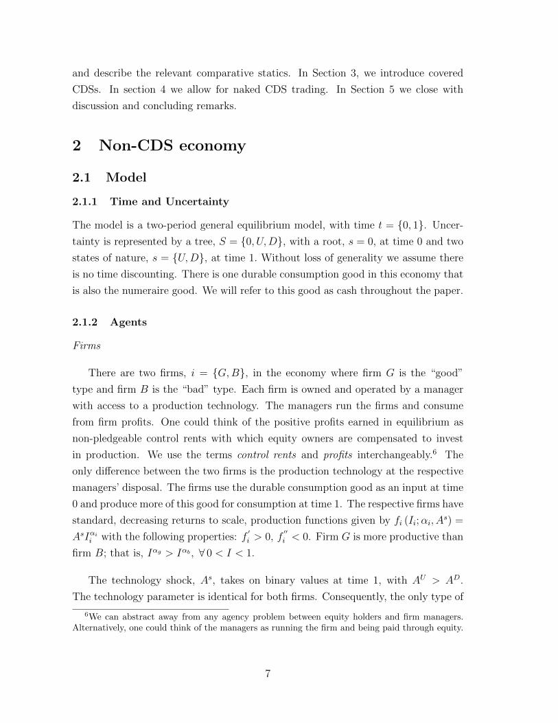
Firms

There are two firms, i = {G,B}, in the economy where firm G is the “good”

type and firm B is the “bad” type. Each firm is owned and operated by a manager

with access to a production technology. The managers run the firms and consume

from firm profits. One could think of the positive profits earned in equilibrium as

non-pledgeable control rents with which equity owners are compensated to invest

in production. We use the terms control rents and profits interchangeably.6 The

only difference between the two firms is the production technology at the respective

managers’ disposal. The firms use the durable consumption good as an input at time

0 and produce more of this good for consumption at time 1. The respective firms have

standard, decreasing returns to scale, production functions given by fi (Ii;αi, As) =

AsIαii with the following properties: f′i > 0, f

′′i < 0. Firm G is more productive than

firm B; that is, Iαg > Iαb , ∀ 0 < I < 1.

The technology shock, As, takes on binary values at time 1, with AU > AD.

The technology parameter is identical for both firms. Consequently, the only type of

6We can abstract away from any agency problem between equity holders and firm managers.Alternatively, one could think of the managers as running the firm and being paid through equity.

7

uncertainty in our model is aggregate.7 Idiosyncratic risk would not have an effect

with two firms and two states, because agents would be able to perfectly insure

themselves. The only way idiosyncratic risk would have an effect is if we considered

more than two states (in which case there would still be non-aggregate risk remaining

even after agents trade with each other).8

For simplicity we normalize the technology shock, AU , to 1. Both firms have

identical knowledge about the quality of their production process, where each firm

knows that s = U arrives with probability γ and s = D with probability (1− γ).

Lastly, firms are competitive price takers in the market for the durable consumption

good.

Investors

We consider a continuum of uniformly distributed risk neutral investors, h ∈ H ∼U (0, 1), who do not discount the future. The absence of time discounting allows us to

focus only on default premiums without loss of generality. Investors are characterized

by linear utility for the single consumption good, xs, at time 1. Each investor is

endowed with one unit of the consumption good, eh = 1, and assigns probability h

to the up state U and (1− h) to the down state D. Thus, a higher h denotes more

optimism and agents agree to disagree. The von Neumann–Morgenstern expected

utility function for investor h is given by

Uh(xU , xD) = hxU + (1− h)xD. (1)

We assume a uniform distribution for tractability. The results will hold in gen-

eral as long as the beliefs are continuous and monotone in h. In terms of investor

preferences, we assume risk-neutrality but the results are also qualitatively preserved

with common investors beliefs and state contingent endowments.

2.1.3 Firm financing

We assume the firms are highly leveraged and optimally raise capital from investors

by issuing debt. Our aim is to better understand the effect of credit derivatives

7It may be natural to think of the model as one of intra-industry debt financing in which twofirms in the same industry are equally affected by a industry specific technology shock.

8We leave this to further research. Also, it is interesting that in considering only aggregate risk,the firms differ only in the productivity and CDSs still have a big effect. With more dimensions ofheterogeneity we predict the effect to be even bigger.

8

Figure 1: Bond payout

𝑝𝑖

ℎ

1 − ℎ

1

𝑑𝑖𝑠 𝑞𝑖

on the debt-issuance decision. The effect of credit derivatives on a more general

capital allocation problem is an interesting natural extension of the model. At time

0, firms issue debt contracts that specify a fixed repayment amount (bonds) and are

collateralized using the pledgeable proceeds from output, which we refer to as cash

flows. The lender (investor) has the right to seize an amount of the collateral up to

the value of the promise, but no more. This enforcement mechanism ensures that

the firm will not simply default on all promises at time 1.

Each bond, priced pi at time 0, promises a face value of 1 upon maturity. The two

firms issue bonds denoted by qi at time 0. In the up state, each bond returns full face

value.9 In the down state bonds pay creditors a deliverable, dsi = min[1,

AsIαii

qi

]. If

debt obligations are not honored, creditors become the residual claimants of the firm

and consume from the cash flows generated from production. Firm borrowing costs,

which are equivalent to bond default premiums because there is no time discounting,

are denoted by ri, and equal to the difference in what the firm owes on maturity

and the amount of capital they receive at the time of issuance, ri =1− pi. Figure 1

depicts the bond payouts.

2.1.4 Firm maximization problem

Each firm chooses an investment amount, Ii, given the market price of bonds to

maximize profits. Since firms have no initial endowment, all their investment for

9We assume the bonds repay in full at s = U to make the model interesting; otherwise, the firmdoes not invest in production.

9

production will have to be financed by issuing debt. Hence Ii = piqi. Let πsi denote

state-contingent firm profits. Firms solve the following program: maxIi

E [πi] ≡ Πi ={γ[AUIαii − qi

]+ (1− γ)

[ADi I

αii − qidDi (qi)

]}s.t. Ii = piqi

(2)

2.1.5 Investor Maximization Problem

We can now characterize each agents’ budget set. Given bond prices pi, each investor,

h ∈ H, chooses cash holdings,{xh0}

, and bond holdings,{qhi}

, at time 0 to maximize

utility given by (1) subject to the budget set defined by:

Bh (pi) ={(xh0 , q

hi , x

hs

)∈ R+ ×R+ ×R+ :

xh0 +∑i

piqhi = eh,

xhs =

(1−

∑i

piqhi

)+∑i

dsiqhi

}, s = {U,D} .

Each investor consumes from two potential sources in either state of nature: con-

sumption based on risk-less asset holdings and consumption based on their total bond

portfolio. In the up state, consumption from bond holdings is equal to the quantity

of bonds an investor owns in his portfolio because each bond has a face value of 1. In

the down state, firms may default on their debt, in which case investors take owner-

ship of the firm and consume from the firms’ available assets on a per0-bond basis.

Furthermore, note that we rule out short sales of bonds by assuming qi ∈ R+.10

2.1.6 Equilibrium

An equilibrium in the non-CDS economy is a collection of bond prices, firm invest-

ment decisions, investor cash holdings, bond holdings and final consumption deci-

sions, pi, Ii, (x0, qi, xs)h∈H ∈ R+×R+× (R+ ×R+ ×R+) such that the following are

10We believe this is not a terribly unreasonable assumption given the known difficulty in borrowingcorporate bonds. CDS markets are far more liquid than secondary bond markets. Furthermore, inthe spirit of Banerjee and Graveline (2014) derivative pricing in our model contains no noise, as willbe clear in the following section, because the investors know technology fundamentals. Banerjeeand Graveline show in proposition 6 that imposing a short-sale ban will have no effect on bondprices when investors can trade in derivatives with no noise.

10

satisfied:

1.

ˆ 1

0

xh0dh+∑i

ˆ 1

0

piqhi dh =

ˆ 1

0

ehdh

2.∑i

ˆ 1

0

qhi dsidh+

∑i

πsi =∑i

AsIαii , s = {U,D}

3. Ii =

ˆ 1

0

piqhi dh

4. πi (Ii) ≥ πi(Ii), ∀Ii ≥ 0 for i = {G,B}

5.(xh0 , q

hi , x

hs

)∈ Bh (pi)⇒ Uh (x) ≤ Uh

(xh), ∀h

Condition (1) says that at time 0 the entire initial cash endowment is held by

investors for consumption or used to purchase bonds from firms. Condition (2)

says the goods market clears at time 1 such that all firm output is consumed either

by firm managers via profits or by creditors via bond payments. Condition (3)

corresponds with the capital market clearing conditions. Condition (4) says that

firms choose investment to maximize profits, and condition (5) states that investors

choose optimal portfolios given their budget sets.

2.2 Bond pricing

We begin by presenting how equilibrium is characterized, which will lay the founda-

tion for analyzing the spillover effects in subsequent sections. We then analyze the

firm investment/production problem in more detail to show how the choice to issue

debt with or with out a positive default premium will also be affected by derivative

trading.

Equilibrium in heterogeneous investor belief models, such as the one employed

here, is based on marginal investors. In equilibrium, as a result of linear utilities,

the continuity of utility in h, and the connectedness of the set of agents, H = (0, 1),

there will be marginal buyers, h1 > h2, at state s = 0. Every agent h > h1 will

buy bonds issued by firm B, every agent h2 < h < h1 will purchase type-G bonds,

and every agent h < h2 will remain in cash. This regime is shown in figure 2. The

marginal buyer indifference between the returns of the various assets available in the

economy will to be crucial in subsequent sections for understanding why introducing

derivatives affects the default premium for all debt contracts in the economy and

11

not just for those contracts on which the derivatives are based. With this, we now

characterize the relationship between the respective firms’ bond prices.

Proposition 1 In any equilibrium without derivatives where both firm types receive

funding and pay positive default premiums, type G bonds are priced higher than type

B bonds.

Proof. See appendix A.

The intuition is simple, in that the asset value of the more productive firm is

always higher than the less productive firm. Debt holders will therefore be willing to

pay a higher price for those bonds, since they are the residual claimants of the assets

given default. Since both bonds pay 1 in full at s = U , more optimistic investors

would rather hold the cheaper of the two assets, which are firm-B bonds. The two

marginal investor indifference equations can be written as:

h1 + (1− h1) dDgpg

=h1 + (1− h1) dDb

pb(3)

h2 + (1− h2) dDg = pg. (4)

Equation (3) says that the more optimistic marginal buyer, h1 will be indifferent

to the expected returns on type-B and -G bonds. Equation (4) says that the less

optimistic marginal buyer, h2, will be indifferent between the return on type-G bonds

and cash. The bond market clearing conditions for type-B and -G bonds require that

the two bond prices be determined by the purchasing power of the respective sets

of investors buying the bonds. That is 1−h1pb

= qb for type-B bonds and h1−h2pg

= qg

for type-G bonds. This characterization clearly shows that bond prices are jointly

determined based on how the marginal investors view the respective returns. A

change in the price of one bond necessarily changes the expected relative return any

investor places on the two assets. For example, an exogenous decrease in the price

makes it more attractive and means it will become strictly preferred to the more

expensive asset unless there is a corresponding change in the relative expected cash

flows to which bond holders are entitled. In equilibrium, as more capital moves to

the cheaper bond from the more expensive bond, the latter’s price must also fall and

will be marginally priced by a less optimistic investor.

2.3 Default premium

12

We now turn to the issue of when it is optimal to issue debt with positive rather

than zero default premium. The maximization problem boils down to choosing an

investment, Ii, that at s = D ensures either repayment or, through limited liability,

that the firm always defaults. In the former, bonds will be priced without risk:

pfi = 1 where the super-script f denotes default risk-free pricing. In the latter case,

bonds will carry a positive risk premium, pρi < 1, where the super-script ρ denotes

a positive risk premium. Let the corresponding profit levels from each of these

investment decisions be denoted by Πfi and Πρ

i . The firm thus chooses I∗i(αi, γ, A

D)≡

arg maxIi

[Πfi ,Π

ρi

]. The first-order conditions for the two investment levels are

Iρi :αiIαi−1i =

1

pρi(5)

Ifi :αiIαi−1i =

1

pfi

(1

γ + (1− γ)AD

). (6)

These are the standard marginal products of capital that must equal the marginal

costs of capital conditions. The default-risk-free condition in (6) takes into account

that all debt is fully repaid at s = U,D through the expected value of the technology

shock, γ + (1− γ)AD.

We begin by analyzing bonds with positive risk premiums. Using (5) and Iρ∗i =

pρ∗i qρ∗i , the bond repayment function, dsi (qρ∗i ), given s = D can be written as

dDi (qi) =AD

αi. (7)

Intuitively, recoverable firm asset values are proportional to the technology shock

parameter, 0 < AD < 1, and the productivity parameter, 0 < αi < 1. The recovery

value also places a natural restriction on the relationship between the two parameters.

Specifically, AD < αi ensures that there is, at least fundamentally, default risk in

the economy. Since αg < αb there are different values of AD for which there is

fundamental default risk for the two firms, 0 < ADG < αG < ADB < αB < 1. As we

show in subsequent discussion, for a given (αG, αB)-pair, whether or not firms issue

bonds with positive default premiums depends on the given(AD, γ

)-tuple.

Turning now to risk-free bonds. Clearly, pf∗i = 1 if firms always repay in all

states. The risk free bond price gives the optimal investment level:

If∗i =[αi(γ + (1− γ)AD

)] 1

(1−αi) = qf∗i . Note that the risk-free bond repayment

13

function, dsi

(qf∗i

)= min

[1,

As(If∗i )αi

qf∗i

]= 1, implies that

AD(If∗i )αi

qf∗i≥ 1. Using (6)

and If∗i = qf∗i gives a relationship between the good state probability, γ, and the

value of the technology shock, ADi , for which issuing risk-free debt is possible even

with fundamental default risk, αi > AD. Formally,

Proposition 2 There is a threshold value of the technology shock, ADi (γ), for any

given state probability, γ. Technology shocks above this threshold allow for risk free

bond pricing. The threshold value of ADi (γ) is an increasing function of γ.


The intuition underlying proposition 2 is that the cash flows from production

must be sufficiently high in bad states (high ADi ) for the firm to always honor its

debt obligations. Additionally, the more likely it is that good states will arrive (high

γ) the more firms invest because doing so increases their expected equity value given

that the face value of debt is always equal to one. This means that cash flows in the

down state must be even higher as γ increases if the firm is to fully honor its debt

obligations.

We must still determine I∗i(αi, γ, A

D)

in equilibrium. We can easily calculate the

different profit levels,{

Πfi

(If∗i

),Πρ

i (Iρ∗i )}

, that determine I∗i . Plugging qf∗i = If∗iinto (2), we obtain

Πf∗i =

(1− αi)αi

qf∗i(ADi (γ) , γ

).

Because debt is always repaid, profits are only affected by state probabilities, γ,

through the affect on bond quantities, qf∗i . Moreover, by proposition 2, an equilibrium

in which risk-free bond pricing exists must be characterized by ADi > ADi (γ) . If

ADi < ADi (γ) , borrowing with a zero default premium is not possible, and profits

are calculated using the optimality condition (5) along with (2):

Πρ∗i = γ × (1− αi)

αiqρ∗i(AD).

Note from (5) that good state probabilities, γ, do not influence the investment levels,

Iρ∗i , when pi < 1 because of limited liability. The firm always invests as if γ = 1

because they always default at s = D; only expected profits are influenced by γ.

Comparing the two expected profit functions, it is clear that if the bond issuances

are the same size(qf∗i = qρ∗i

)firms would always prefer the risk-free investment level.

14

Equilibrium debt contracts characterized by positive default premiums must allow

the firm to invest more than debt contracts that are risk free do, and the difference

in the two amounts is proportional to the likelihood that the equity claimants retain

positive equity γ, γ >qf∗iqρ∗i

. Lastly, note that the only interesting range of technology

shocks for analyzing a tradeoff between the two different debt issuances is AD ∈[ADi , αi

). All shocks below ADi result in positive default premiums, q∗i = qρ∗i , and all

shocks above αi result in risk free bond pricing, q∗i = qf∗i . The following proposition

characterizes the parameter regions over which firms issue the two different types of

bonds.

Proposition 3 Firms will always issue bonds with positive default premium when

ADi < ADi and will always issue bonds risk free for ADi ≥ αi. For AD ∈[ADi , αi

)firms issue bonds risk free if and only if γ < γ.

This result says that for intermediate values of stochastic cash flows, firms must

optimally choose between debt for which they can always repay and debt that carries

a positive default premium and will not be repaid when cash flows are low. Firms

may only issue debt without (with) credit risk in this region if the likelihood that

cash flows are good is sufficiently low (high) because when good cash flow states are

likely, the default premium to issue debt will be lower, which incentivizes raising

more capital that cannot be repaid if bad states arrive. Alternatively, when good

cash flow states are less likely, the default premium will be higher, which incentivizes

issuing smaller amounts of debt that can repaid given bad news.

Example 1{AD = 0.2, γ = 0.5, αG = 0.5, αB = 0.65

}This example gives results for default premiums, marginal buyers, and the re-

mainder of the endogenous variables in the economy for the listed parameters. Fig-

ure 2 is the marginal buyer equilibrium characterization and table 1 gives the values

of the endogenous variables. The values of the technology thresholds for determin-

ing whether default risk free bonds may be issued for γ = 0.5 are ADG = .33 and

ADB = .4814, and clearly pi < 1, i = G,B. The comparative statics for bond pricing

and investment are not particular to the parameters chosen so long as AD < ADG .

Higher values of the technology shock naturally raise bonds prices, investment and

control rents/profits. However, increases in the technology shock above the respec-

tive thresholds, ADi , will change the comparative statics since the respective bond

prices will be pi = 1.

15

Figure 2: Non-CDS economy

Type B Bond Buyers

Type G Bond Buyers

Cash

h1 = .8471

h2 = .6831

h = 0

h =1

Table 1: Equilibrium values: Non-CDS economy

non-CDS economyi = G i = B

Price: pi .8099 .7973Quantity: qi .2025 .1918

Investment: Ii .1640 .1529Output: Y U

i .4049 .2950Exp.Profit: E [πi] .1012 .0516

16

3 Covered CDS economy

In this section, we incorporate CDSs into the baseline model. A CDS is a financial

contract in which the CDS seller compensates the buyer for losses to the value of

an underlying asset for a specified credit event or default. The underlying assets in

this economy are firm bonds. CDS contracts compensate buyers with the difference

between a bond’s face value at maturity and its recovery value at the time of the

credit event. Thus, CDS allow investors to hedge against idiosyncratic default risk.11

We first consider covered CDSs, in which buyers are required to also hold the

underlying asset (that is, that bond for whom the CDS is written). We assume the

seller must post enough collateral to cover the payment in the worst case scenario to

rule out any counter-party risk. Let qhic be the number of CDSs that investor h can

sell, and let pic be the CDS price. Therefore, the total cash that investor h holds to

collateralize CDS contracts, including payments received for selling CDSs, will equal

the maximum possible CDS payout in the event of firm default, times the number of

CDS contracts sold:

1 + pic qic = qhic (1− dsi ) . (8)

Solving for the total number of CDS contracts gives

qhic =1

1− dsi − pic. (9)

Figure 3 shows the payout to the CDS seller and buyer. At time 0, a CDS seller

must post a portion of his own collateral, 1−dsi −pic, to insure each CDS. At s = U ,

the CDS seller consumes the collateral, as the bond pays in full. At s = D, all of

the collateral is used to compensate CDS buyers. Thus, selling CDSs is equivalent

to holding an Arrow-Up security, as it pays out only when s = U .

11CDS do not allow investors to insure away aggregate risk.

17

Figure 3: Covered CDS payout

𝑝𝑖 + 𝑝𝑖𝑐=1

ℎ

1 − ℎ

11 − 𝑑𝑖𝑠 𝑞𝑖

1

ℎ

1 − ℎ

0

1 − 𝑑𝑖𝑠 𝑞𝑖 − 𝑝𝑖𝑐

CDS Seller Covered CDS Buyer

3.1 Investor maximization problem

Given bond and CDS prices, (pi, pic), each investor h decides on cash, bond and CDS

holdings,{xh0 , q

hi , q

hic

}, to maximize utility (1) subject to the following budget set:

Bh (pi, pic) ={(xh0 , q

hi , q

hic, x

hs

)∈ R+ ×R+ ×R×R+ :

xh0 +∑i

piqhi +

∑i

picqhic = eh,

xhs = xh0 −∑i

picqhic +

∑i

qhi dsi +∑i

qhic (1− dsi ) , s = {U,D}

max{

0, qhic}≤ qhi

}.

The first two equations are analogous to the investor budget set in the non-CDS

economy. The third equation states that since CDS buyers are required to hold the

underlying asset, the maximum number of CDS contracts that can be purchased

cannot exceed the number of bonds owned. Note that there is no sign restriction

on qhic. Selling CDS implies that qhic < 0, while qhic > 0 implies purchasing CDS.

Short selling of bonds is still ruled out by the restriction qi ∈ R+ as in the non-CDS

economy.

18

3.2 Equilibrium

An equilibrium in the covered-CDS economy is a collection of bond prices, CDS

prices, firm investment decisions, investor cash holdings, bond holdings, CDS hold-

ings and final consumption decisions,

pi, Ii, (x0, qi, qic, xs)h∈H ∈ R+×R+×(R+ ×R+ ×R×R+), such that the following

are satisfied:

1.

ˆ 1

0

xh0dh+∑i

ˆ 1

0

piqhi dh =

ˆ 1

0

ehdh

2.∑i

ˆ 1

0

qhi didh+∑i

πsi =∑i

AsIαii , s = {U,D}

3.

ˆ 1

0

qhic = 0

4. Ii =

ˆ 1

0

piqhi dh

5. πi (Ii) ≥ πi(Ii), ∀Ii ≥ 0

6.(xh0 , q

hi , q

hic, x

hs

)∈ Bh (pi, pic) =⇒ Uh (x) ≤ Uh

(xh), ∀h

Condition (1) states that all of the initial endowment is either held by investors

or used to purchase bonds. Condition (2) says the goods market clears such that

total firm output is consumed by firm managers via profits and used to repay bond

holders. Condition (3) says that the CDS market is in zero net supply, while (4)

states that the capital market clears. Condition (5) says firms choose investment to

maximize profits. Lastly, (6) states that investors choose a portfolio that maximizes

their utility, given their budget set.

We make use of the following lemma to characterize equilibrium in the covered

CDS economy.

Lemma 1 If 0 < dDi (qi) < 1, then no bonds for which CDS are sold will be purchased

without CDS.

Proof: See appendix B.

The intuition behind lemma 1 is that any investor optimistic enough to buy a

bond without a CDS will be better off selling CDSs on that bond. Additionally, if

the recovery value of the bond is zero, then CDSs and bonds pay the same amount

19

in both states, thus making CDSs redundant assets. Finally, if the recovery value of

the bond is 1, then bonds are risk free and no CDSs will trade in equilibrium.

3.3 Borrowing costs and spillovers

We introduce CDSs only on one firm’s debt to establish the borrowing cost spillover

result. For expositional purposes, let investors issue CDSs on firm-B debt.12 As in

the non-CDS economy, there will be marginal buyers, h1 > h2. In equilibrium, every

agent h > h1 will sell CDSs on type-B debt, every agent h2 < h < h1 will purchase

type-G debt, and every agent h < h2 is indifferent to holding covered CDS and cash.

More specifically, agents h < h2 hold a portfolio of covered positions on type-B and

cash.13 Compared with the non-CDS economy, covered CDSs lower borrowing costs

for the firm on which CDSs are traded—firm B, because the derivative allows the

optimists who believe firms will always repay their debt to hold all of the credit

risk. Because CDS sellers only have to hold a portion of their collateral to cover the

expected loss given default, which is always less than the price of the bond, each

individual CDS seller can hold more credit risk than they could when just buying

bonds. The resulting marginal buyers are therefore more optimistic than in the

economy with out CDSs. The marginal buyer indifferent equations are now

h1

(1− dDb

)1− pbc − dDb

=h1 + (1− h1) dDg

pg(10)

h2 + (1− h2) dDg = pg. (11)

The CDS sellers’ aggregate purchasing power to price CDSs is now (1−h1)

1−pbc−dDb= qb.

The purchasing power of the marginal type-G bond buyers takes the same form as the

non-CDS economy: h1−h2pg

= qg, with different marginal buyers. Lastly, because some

agents hold a portfolio of covered CDS and cash, a non-arbitrage pricing condition

between the CDS and bond market links the price of credit risk in the CDS market

with the default premium in the bond market: pbc + pb = 1. Consistent with Che

12The qualitative results for borrowing cost spillovers and endogenous positive default premiumsare not particular to the firm’s debt from which the CDSs derive their value. Endogenizing CDSissuance is an interesting question, but beyond the scope of this paper. Work by Banerjee andGraveline (2014), Bolton and Oehmke (2011), and Oehmke and Zawadowski (2015b) provides nicereference points for thinking about why we see CDSs emerge on some firms and not others.

13In equilibrium, every agent h < h2 will be indifferent between cash and a covered position andeach agent will hold a portfolio consisting of 30.43% in covered positions and the rest in cash, forthe same parameters chosen in example 1. To compute this portfolio allocation we simply dividethe number of type B bonds investors hold by their total cash endowment, qb

h2.

20

and Sethi (2015), but with a twist, we have the following bond pricing implications:

Proposition 4 Covered CDSs raise bond pricing for the firm for whom CDSs are

written.

Proof. See appendix B.

More interestingly, because our model has an additional asset with a different

fundamental valuation based on heterogeneous but correlated cash flows, there are

general equilibrium borrowing cost implications for firm G even though investors do

not trade CDSs on firm-G debt.

Corollary 1 The default premium for a firm without CDSs trading is affected by

CDSs trading on other firms with correlated cash flows.


This result follows directly from proposition 4 because the marginal CDS seller

who prices the credit risk for firm B is more optimistic than the corresponding

marginal bond buyer in the non-CDS economy. Because each CDS seller buys credit

risk using collateral in the amount equal to the loss given default of the underlying

bond contract, a given set of investors of size (1− h1) in the non-CDS economy have

more purchasing power to buy credit risk in the covered CDS economy. Firm G,

competing with firm B to raise capital from optimistic investors, can therefore issue

debt to more optimistic set of investors than in the non-CDS economy, as well. This

increase in the set of investors financing both firms’ debt issuances raises bond prices

for firm G.

The fact that cash flows are correlated across good and bad states is also impor-

tant. Take the limiting example in which firm G’s cash flows are high at s = D and

low at s = U . The firm would then find it optimal to issue debt to those investors

most willing to pay for an asset whose payouts are most correlated with their subjec-

tive beliefs. Firm G would then prefer to issue debt to pessimists who would pay a

higher price for an asset that pays more at t s = D with certainty than to optimists

who would pay high prices for high payouts in the exact opposite states. It is this in-

terpretation of the model that leads naturally to an intra-industry or geographically

limited model of debt financing. Firms in the same industry or geographic area may

21

Figure 4: Type-B covered CDS economy

Type B CDS Sellers

Type G Bond Buyers

Cash

h1 = .8823

h2 = .7114

h = 0

h =1

be more likely to default in similar states than firms in completely different indus-

tries or regions. Moreover, the recent empirical findings in Li and Tang (2016) on the

leverage and borrowing of intra-industry firms are consistent with this interpretation

of the model. Figure 4 and table 2 show the corresponding marginal buyer regimes

and endogenous variables in the economy for the same parameters as in example 1.

Note that even though the CDS trades on firm B, the price of firm G debt rises from

pG = .8099 to pG = .8269. For the same parameters as in example 1, Figure 5 shows

the equilibrium shift in the set of investors financing firm G’s debt issuance in the

non-CDS economy and the covered CDS economy with CDSs only trading on firm

B.

Table 2: Equilibrium values: Type-B covered CDS economy

Type B Covered CDS Economyi = G i = B



i .4134 .3331Exp.Profit: E [πi] .1034 .0583

22

Figure 5: Covered CDS economy: Type-G positive spillover

.88

h = 0

h =1

.70.72

.87 Investors financing Type G in ‘Type B

Covered CDS Economy’ Investors financing Type G in ‘Non-‐CDS

Economy’

3.4 CDSs and credit risk

In this section we show that the increase in bond pricing attributed to CDS trading

also induces firms to issue debt that carries a positive default premium for more values

of the down state probability than in the non-CDS economy. As shown in appendix

A for proposition 2, the threshold values of ADi above which issuing default-risk-free

debt is possible are determined only by parameters γ and αi. CDSs do not change

any of the fundamentals of the economy, so the threshold values are the same as in

the non-CDS economy. What does change is the cost of issuing debt with a positive

default premium and hence the relative costs and benefits of issuing such debt claims.

To see how CDSs affect the extensive default premium choice margin, recall that

the necessary and sufficient condition to issue debt with a positive default premium is

that the debt must yield higher control rents to equity claimants, which can be simply

expressed through the optimal debt issuance levels of the two debt contracts: γqρ∗i >

qf∗i , where the hat corresponds to the non-CDS economy quantities. The left-hand

side is the expected control rent associated with issuing debt with positive default

premium and the right-hand side is the control rent from issuing debt that is always

repaid. Because the default-risk-free contract is purely a function of fundamentals,

the right-hand side of the inequality remains unchanged. From proposition 4 we

know that firms borrow at lower borrowing costs and issue more bonds when CDSs

23

trade. Thus, if there is a γ < 1 for which γqρ∗i = qf∗i in the non-CDS economy, then

γqρ∗i > qf∗i in the covered CDS economy and γ > γ ≡ γqρ∗i = qf∗i , where the tildes

denote covered CDS economy variables. The decrease in the threshold γ in covered

CDS economies above which firms issue risky debt establishes the first result of the

trade-off between borrowing costs and default risk in CDS economies.

Proposition 5 Give bad states, CDS contracts that lower the default premium of

the underlying bond contract will tend to increase the likelihood that default occurs

in equilibrium. For any value of ADi ∈[ADi , αi

)firms will issue default-risk free debt

contracts if and only if γ ≤ γ < γ.

The endogeneity of production in the economy helps establish this result. In

Che and Sethi (2015), covered CDS also lower borrowing costs, but they increase

the ability to repay debt for any given investment level. The positive relationship

between covered CDSs and ability to repay debt would be true in our model if Ii

were fixed. When endogenized however, firms respond to bond pricing by issuing

more debt. Because production rents are only captured in the up state when the

debt raised to produce carries a positive default premium, a decrease in default

premiums raises the resulting profitability from issuing these debt contracts, even

though fundamentals do not change. If, in expectation, there was a state probability

in the non-CDS economy for which the firm was indifferent between issuing either

debt contract, the debt contract with a positive default premium would be strictly

preferred. The decrease in default premiums and increase in investment are offset

by the increase in default incidence at s = D.

4 Naked CDSs

In this section, we extend the model by allowing investors to hold naked CDS po-

sitions: investors do not need to hold the underlying asset to purchase a CDS. A

naked CDS buyer expects to receive the difference between the face value of the bond

and its value at the time of default. The naked CDS payout structure is given in

figure 6. Furthermore, notice that buying a naked CDS is equivalent to buying the

Arrow-down security, since it pays out only when s = D.

At time 0. an investor can purchase a naked CDS by paying pic. The buyer

believes with probability h that the up-state will occur at time 1, the firm will not

24

Figure 6: Naked CDS payout

𝑝𝑖𝑐

ℎ

1 − ℎ


ℎ

1 − ℎ

0

1 − 𝑑𝑖𝑠 𝑞𝑖 − 𝑝𝑖𝑐

CDS Seller Naked CDS Buyer


default, and the CDS will not payout. The buyer believes with probability (1− h)

that the downstate will occur at time 1. In this case, the buyer expects to receive the

difference between the face value of the bond and its recovery value, (1− dsi ). We

continue to assume that CDS sellers post enough collateral to cover payments in the

worst-case scenario. Therefore the maximum CDS payout carries over from previous

economies and is given by equation (9). Moreover, the implications of lemma 1 still

hold and no bond is bought without credit protection if CDSs trade on that bond.

4.1 Investor maximization problem

Given bond and CDS prices (pi, pic), each investor chooses cash, bond, and CDS

holdings,{xh0 , q

hi , q

hic

}, to maximize utility (1) subject to the budget set:

Bh (pi, pic) ={(xh0 , q

hi , q

hic, x

hs

)∈ R+ ×R+ ×R×R+} :

xh0 +∑i

piqhi +

∑i

picqhic = eh,

xhs = xh0 −∑i

picqhic +

∑i

qhi dsi +∑i

qhic (1− dsi )}.

The investor’s budget set is exactly the same as the one described in the covered CDS

economy except that investors can now buy CDS without holding the underlying

25

asset. Hence there is no restriction tying the maximum number of CDS contracts

bought to the number of bonds held.

Equilibrium existence and institutional investor

Fostel and Geanakoplos (2014) identify an existence problem in production economies

wherein collateral equilibrium may breakdown in the presence of naked CDS. In an

earlier working paper version of their paper, Che and Sethi (2010) assume that a

retail investor will always demand bonds so that equilibrium does not break down.

We follow this assumption to compute equilibrium. Lastly, the presence of the in-

stitutional investor would not affect equilibrium in the non-CDS and covered-CDS

economies. Limiting the investor’s risk exposure of the investor will prevent it from

purchasing bonds without any CDS protection. Thus the investor will remain in cash

in an economy without CDS. Moreover, in the covered CDS economy, agents who did

not sell CDS held a portfolio of cash and covered CDS positions. The institutional

investor could just as easily replace the agents’ covered CDS positions, leaving them

only holding cash and the equilibrium unperturbed.14

4.2 Equilibrium

An equilibrium in the naked-CDS economy is a collection of bond prices, CDS prices,

firm investment decisions, and investor consumption decisions,

pi, pic, Ii, (x0, qi, qic, xs)h∈H ,(xM0 , x

Ms

)∈ R+×R+×R+× (R+ ×R+ ×R×R+)×

(R+ ×R+),

14A formal presentation of the retail investor problem is presented in appendix C.

26

such that the following are satisfied:

1.

ˆ 1

0

xh0dh+ xM0 +∑i

piqMi +

∑i

picqMic =

ˆ 1

0

ehdh+ eM

2.∑i

qMi +∑i

πsi =∑i

AsIαii , s = {U,D}

3.

ˆ 1

0

qhicdh+ qMi = 0

4.Ii = piqMi

5.πi (Ii) ≥ πi(Ii), ∀Ii ≥ 0,

6.(xh0 , q

hi , q

hic, x

hs

)∈ Bh (pi, pic)⇒ Uh (x) ≤ Uh

(xh), ∀h

7.(cMi)∈ BM (pi, pic)⇒ UM (c) ≤ Uh

(cM)

Condition (1) states that all endowments, including the retail investor’s, go to one

of three uses: (a) held as collateral to issue CDSs, (b) held by the retail investor for

consumption, or (c) used by the retail investor to purchase bonds and covered CDSs.

Condition (2) says the goods market clears such that total firm output is consumed

by firm managers in the form of profits and is used to repay bond holders. Condition

(3) says that the CDS market is in zero net supply because all CDSs purchased as

naked investments or by the retail investor as covered investments will be equal to all

of the CDS issued. Condition (4) is the capital market clearing condition. Condition

(5) says firms choose investment to maximize expected profits. Condition (6) states

that investors choose a portfolio that maximizes their utility given their budget sets,

and condition (7) says that the retail investor holds a portfolio that maximizes his

utility given his budget set.

4.3 Borrowing costs and spillovers revisited

In this section, we show that the borrowing cost spillovers are also present in the

naked CDS economy. To keep the examples comparable across economies, we con-

tinue to examine an economy for which CDSs trade only on firm-B debt. As before,

there will be marginal buyers, h1 > h2. In equilibrium, every agent h > h1 will sell

CDSs on typeB debt, every agent h2 < h < h1 will purchase bonds issued by type G,

and every agent h < h2 will buy naked CDSs on type-B debt. Naked CDSs raise type

B’s borrowing costs because pessimists are able to purchase Arrow-Down securities

created through the CDS contract, which increases the price a CDS seller receives

27

for selling such contracts. As the price increases, investors can further leverage their

cash endowments because they have to hold less of their own capital to issue CDSs.

The resulting marginal CDS sellers are now more pessimistic than the bond buyers

in the non-CDS economy. The marginal buyer indifference equations in the naked

CDS economy are:

h1

(1− dDb

)pb − dDb

=h1 + (1− h1)dDg

pg(12)

(1− h2)(1− dDb

)1− pb

=h2 + (1− h2)dDg

pg. (13)

Note here that firm-G bonds are priced by two separate investors. The more opti-

mistic investor, h1, is indifferent between selling a CDS on firm-B debt and buying

firm-G bonds in (12). The more pessimistic investor, h2, is indifferent between buy-

ing a CDS on firm-B debt and buying firm-G bonds in (13). This wedge between

the Arrow-Up and the Arrow-Down securities means even though the arrow claims

are traded, the Arrow-Debreu equilibrium is not established in this economy, as in

Fostel and Geanakoplos (2012). The market-clearing conditions that establish the

total purchasing power investors have to clear the markets are (1−h1)

1−pbc−dDb=(qb + h2

pbc

)for the CDS market on firm B and (h1−h2)

pg= qg for the bond market on firm G .

Lemma 1 from the covered CDS economy continues to hold, implying that no bonds

on which CDS are traded will be purchased without insurance. Furthermore, we

derive the following lemma to solve for equilibrium in the naked CDS economy.

Lemma 2 Only the institutional investor holds cash or covered assets in equilibrium.


The intuition for the optimists holds from lemma 1. The for pessimists, any

investor pessimistic enough to remain in cash will be better off buying a naked

CDS. Thus, only the institutional investors hold risk-free assets. The borrowing cost

implications for the economy are similar to those in Fostel and Geanakoplos (2012

and 2016) and Che and Sethi (2015) and are summarized in the following proposition.

Proposition 6 Naked CDS lower bond prices for the firm for whom CDS are writ-

ten.


28

Figure 7: Type-B naked CDS economy

Type B CDS Sellers

Type G Bond Buyers

Type B (Naked) CDS Buyers

h1 = .5589

h2 = .4484

h = 0

h =1

As described above, the derivative markets attracts more optimists to sell CDS

as pessimists bid up the prices of derivative contracts. This “capital reallocation

channel” is common to a class of heterogeneous agent models used to analyze CDS

and bond market pricing (see Fostel and Geanakoplos (2012 and 2016), Che and

Sethi (2015), and Oehmke and Zawadowski (2015) for other examples). What is

new in our model in terms of borrowing cost implications, is, once again, the fact

that firm G will also be affected by the movement of capital from bond market

purchases to collateralizing derivative contracts because firm G’s cash flows from

production are correlated with firm B’s. Figure 7 and table 3 show the marginal

buyer characterization of equilibrium and the values of the endogenous variables for

the same parameters used in the non-CDS and covered CDS Economies. Figure 8

shows the shift in marginal investors financing firm-G debt in the naked CDS and

covered CDS economies.

Table 3: Equilibrium values: Type-B naked CDS economy

Type B Naked CDS Economyi = G i = B



i .3170 .1950Exp.Profit: E [πi] .0793 .0341

29

Figure 8: Naked CDS economy: Good firm negative spillover

.88

h = 0

h =1

.45

.71

.55

Investors financing Type G in ‘Type B

Covered CDS Economy’

Investors financing Type G in ‘Type B

Naked CDS Economy’

4.4 CDS and default risk revisited

As with the covered CDS economy, the default-risk-free contract is unchanged. The

debt levels that are sustainable and permit firms to fully honor debt obligations in all

states are driven by economy fundamentals,(αi, γ, A

D). Therefore, the change in the

default premium associated with issuing a risky debt contract alters the extensive

margin between risky and risk-free contracts. Using proposition 6, we know that

default premiums increase in the naked CDS economy and firms respond by issuing

less debt, qρi < qρi , where hats denote the risky bond quantity in the non-CDS

economy and dots denote the equivalent in the naked CDS economy. Thus, for a

given state realization in which γqρi = qf∗i holds in the non-CDS economy, γqρi < qf∗iwill hold in the naked CDS economy.

Proposition 7 Given bad states, CDS contracts that raise the default premium of

the underlying bond contract will tend to decrease the likelihood that default occurs in

equilibrium. For any value of ADi ∈[ADi , αi

), firms will issue default-risk-free debt

contracts if and only if γ ≥ γ > γ.

Propositions 5 and 7 show that the effect on default premiums and endogenous

investment of trading CDSs can be counterbalanced by the effect on the decision to

issue risky rather than risk-free debt. On the one hand, CDS contracts allow the

leveraging of cash, which changes the demand for bonds and the default premiums

30

at which firms issue risky debt. Risk-free debt contracts, on the other hand, are

determined by fundamental technology processes and state probabilities, and they

are therefore unaffected by the presence of derivative trading. The fact that derivative

trades affect default premiums when firms issue risk debt implies that the relative

incentives to choose between debt contracts that do or do not contain default risk are

altered even when fundamentals do not change. Thus, financial innovation through

derivative trading may effect not only the intensive margin and how much debt to

issue, but the extensive margin of whether debt contracts contain default risk.

5 Discussion and concluding remarks

Credit derivatives can induce a tradeoff between firm borrowing costs and default

probability. Lower default premiums incentivize investment for which debt obliga-

tions are not met in states characterized by negative productivity shocks. Alterna-

tively, higher default premiums lead to debt financing that firms are more likely to

repay for given productivity shocks. Financial instruments that effect default pre-

miums can induce such a tradeoff even when nothing fundamental changes in the

economy. In terms of our model, the set of parameters(γ, AD

)in the different

economies for which each firm defaults changes as CDS are introduced.

Figure 9 illustrates the effect covered CDSs have on default relative to the non-

CDS economy. The parameters are those chosen for example 1 throughout the paper.

The diagram shows the different possible default regimes. The area labeled “full risk

regime” is the set of parameter values for which both firms default when s = D.

Similarly, “partial risk regime” corresponds to the region where only type-B defaults,

and neither firm defaults in the “risk free regime.” The individual cells outlined and

labeled “default G” and “default B” highlight the impact of introducing covered

CDSs. For example, relative to the non-CDS economy, all of the default B cells

indicate that firm B defaults on its debt obligations. Likewise, relative to the non-

CDS economy, all of the default G cells indicate that firm G defaults on its debt

obligations. The likelihood of s = U given by γ is on the vertical axis (increasing

γ moving downward) and the value of the technology shock, AD, on the horizontal

(increasing AD going from left to right).

You can see that for a given ADi in which borrowing risk free is possible, firm

B defaults in the down state for more values of γ (the gray default B cells would

31

Figure 9: Increased default risk: Non-CDS versus covered CDS

Gamma/AD 0.05 0.10 0.15 0.20 0.25 0.30 0.35 0.40 0.45 0.50 0.55 0.60 0.65 0.70 0.75 0.80 0.85 0.90 0.95 1.00 0.05 0.10 0.15 DEFAULT:G 0.20 DEFAULT:B 0.25 DEFAULT:B 0.30 DEFAULT:G DEFAULT:B 0.35

FULL RISK REGIME

PARTIAL RISK REGIME

DEFAULT:B

RISK FREE REGIME

0.40 DEFAULT:B 0.45 DEFAULT:B 0.50 DEFAULT:B 0.55 DEFAULT:B 0.60 DEFAULT:B 0.65 DEFAULT:B 0.70 DEFAULT:B 0.75 DEFAULT:B 0.80 DEFAULT:G 0.85 0.90 0.95 1.00

be black in the non-CDS economy).15 The associated increase in default risk in the

covered CDS economy is consistent with the empty creditor story. However, our

mechanism is novel and does not rely on a maturity mis-match between firm assets

and liabilities or rollover risk and coordination problems. Covered CDS can increase

default risk through the pricing incentives to issue debt that defaults in bad times

even when assets and liabilities are perfectly aligned and no maturity-mismatch is

present. Additionally, the model shows that having an insurable interest and owning

the CDS on that interest (covered) leads to very different default implications than

taking a speculative position (naked). Current empirical studies cannot distinguish

between covered and naked positions at the CDS-counterparty level and thus only

test the covered story of the empty creditor problem.

Figure (10) shows the equilibrium comparing the covered CDS and naked CDS

economies for the parameters used in example 1. It is the analogue to figure 9 in that

it shows the effect of introducing naked CDSs when CDSs already exist. We make

this comparison to show the effect on default of banning naked CDS; presumably,

covered CDS would still be allowed. The cells labeled “No Def G” indicate that firm

G switches from defaulting on debt obligations in covered CDS economies to fully

repaying when naked CDS are introduced. Similarly, the cells labeled “No Def B”

indicate that firm B switches from defaulting on debt obligations in covered CDS

economies to fully repaying when naked CDS are introduced. In contrast to the

15The default effect on firm B is more pronounced in this example because the derivative isintroduced on firm B. Still, there is a spillover default effect on firm G as well.

32

Figure 10: Decreased default risk: Covered CDS versus naked CDS

Gamma/AD 0.05 0.10 0.15 0.20 0.25 0.30 0.35 0.40 0.45 0.50 0.55 0.60 0.65 0.70 0.75 0.80 0.85 0.90 0.95 1.00 0.05 NO-‐DEF:G NO-‐DEF:B 0.10 NO-‐DEF:G NO-‐DEF:B 0.15 NO-‐DEF:G NO-‐DEF:B 0.20 NO-‐DEF:G NO-‐DEF:B NO-‐DEF:B 0.25 NO-‐DEF:G NO-‐DEF:B NO-‐DEF:B NO-‐DEF:B 0.30 NO-‐DEF:G NO-‐DEF:B NO-‐DEF:B NO-‐DEF:B 0.35

FULL RISK REGIME

NO-‐DEF:G

PARTIAL RISK REGIME

NO-‐DEF:B NO-‐DEF:B

RISK FREE REGIME

0.40 NO-‐DEF:G NO-‐DEF:B NO-‐DEF:B NO-‐DEF:B 0.45 NO-‐DEF:B NO-‐DEF:B 0.50 NO-‐DEF:B NO-‐DEF:B 0.55 NO-‐DEF:B 0.60 NO-‐DEF:B 0.65 NO-‐DEF:B 0.70 NO-‐DEF:B 0.75 0.80 NO-‐DEF:G 0.85 0.90 0.95 1.00

previous example, there are fewer values of γ for which the firms default. These

results highlight the tradeoff between borrowing costs and default risk not identified

in the extant CDS literature.

We further show, through the capital reallocation channel other models have

highlighted, that when the productive assets on which CDSs trade have correlated

cash flows, the returns between the debt contracts that finance the assets must be

equal in equilibrium. This equality leads to spillover effects even as CDS markets

do not exist on all underlying assets. The spillover effects include changes in bond

pricing, investment demand, and default risk. Thus, our model provides a new

mechanism through which to think about the empirical results on the leverage and

investment externalities of CDS trading identified by Li and Tang (2016).

33

References

[1] Acharya, Viral and Timothy Johnson, (2007). “Insider Trading in Credit Deriva-

tives.” Journal of Financial Economics. 84, 110-141.

[2] Ashcraft, Adam and Joao Santos, (2009) “Has the CDS Market Lowered the

Cost of Corporate Debt?”, Journal of Monetary Economics, 56, 514-523.

[3] Augustin, Patrick, Marti Subramanyam, Dragon Yongjun Tang, and Sara Qian

Wang, (2014). “Credit Default Swaps: A Survey.” Foundations and Trends R© in

Finance. vol 9, No 1-2, 1-196.

[4] Banerjee, Snehal and Jeremy Graveline, (2014). “Trading in Derivatives when

the Underlying is Scarce.” Journal of Financial Economics. 111, 589-608.

[5] Bernanke, Ben, (2008), “The Future of Mortgage Finance in the United States.”,

Address at UC Berkeley/UCLA Symposium: The Mortgage Meltdown, the

Economy and Public Policy, Berkeley, California.

[6] Bolton, Patrick and Martin Oehmke (2011), “ Credit Default Swaps and the

Empty Creditor Problem.”, Review of Financial Studies, 24 (8), February 2011.

[7] Che, Yeon-Koo and Rajiv Sethi, (2015) “Credit Market Speculation and the

Cost of Capital,” American Economic Journal: Microeconomics. 6(4), 1-34.

[8] Danis, Andras and Andrea Gamba, (2015). “The Real Effects of Credit Default

Swaps.” Working Paper.

[9] Financial Times, (2011), “Bankers Fear Political Motives Will Kill Off CDS”

David Oakley and Tracy Alloway. Capital Markets, October, 25, 2011

[10] Fostel, Ana and John Geanakoplos, (2016), “Financial Innovation, Collateral

and Investment.” American Economic Journal: Macroeconomics. 8(1), 242-84.

[11] Fostel, Ana and John Geanakoplos, (2012), “Tranching, CDS, and Asset Prices:

How Financial Innovation Can Cause Bubbles and Crashes.” American Eco-

nomic Journal: Macroeconomics, Vol. 4, no 1, 190-225.

[12] Kim, Gi, (2013). “Credit Default Swaps, Strategic Default and the Cost of

Corporate Debt.” Working Paper.

34

[13] Kim, Jae, Pervin Dushyantkumar, Shroff Vyas ,and Regina Wittenberg-

Moerman, (2014). “Active CDS Trading and Managers’ Voluntary disclosure,

Working Paper. University of Chicago.

[14] Geanakoplos, John, (2010), “The Leverage Cycle,” In NBER Macroeconomics

Annual 2009. Vol 24 edited by Daron Acemoglu, Kenneth Rogoff, and Michael

Woodford, 1-65. Chicago: University of Chicago Press.

[15] Li, Jay and Dragon Youngjun Tang, (2016). “The Leverage Externalities of

Credit Default Swaps.” Forthcoming: Journal of Financial Economics.

[16] Morrison, Alan, (2005). “Credit Derivatives, Disintermediation, and Investment

Decisions.” Journal of Business. 78(2), 621-648.

[17] Norden, Lars, Consuelo Silva Buston and Wolf Wagner (2014). “Financial In-

novation and Bank Behavior: Evidence from Credit Markets.” Journal of Eco-

nomic Dynamics and Control. vol. 43, 130-145.

[18] Norden, Lars, and Kristina Radoeva, (2013). “What do We Know about Spec-

ulation in the CDS Market?” Working Paper. Midwest Finance Association

2013.

[19] Oehmke, Martin and Adam Zawadowski, (2015a). “Synthetic or Real? The

Equilibrium Effects of Credit Default Swaps on Bond Markets” Review of Fi-

nancial Studies 28(12), 3307-3337.

[20] Oehmke, Martin and Adam Zawadowski, (2015b). The Anatomy of the CDS

Market” Forthcoming: Review of Financial Studies.

[21] Parlour, Christine and Andrew Winton, (2013). “Laying Off Credit Risk: Loan

Sales Versus Credit Default Swaps.” Journal of Financial Economics. vol. 107,

25-45.

[22] Shan, Susan, Dragon Yongjun Tang, and Andrew Winton, (2015). “Market

Versus Contracting: Credit Default Swaps and Creditor Protection in Loans.”

Working Paper.

[23] Subrahmanyam, Marti, Dragon Yongjun Tang, and Sara Qian Wang, (2014).

“Does the Tail Wag the Dog? The Effect of Credit Default Swaps on Credit

Risk.” Review of Financial Studies. 27(10). 2927-2960.

35

A Appendix

A.1 Partial-Risk

A.1.1 Non CDS Equilibrium

This equilibrium is characterized by the fact that Firm G is always able to fully

repay its debt while the bad firm defaults when s = D. This equilibrium will be

characterized as a combination of the Risk-Free Regime presented in the preceding

section and the Full-Risk Regime described in Section 2.2.

The system of equations that characterizes equilibrium in the non-CDS economy

includes eight endogenous variables (pi, qi, Ii, h1, h2) and is as follows:

1.h1 + (1− h1) dDb = pb

2.h2 + (1− h2) = pg

3.αgIαg−1g =

1

[γAU + (1− γ)AD]

4.αbIαb−1b =

1

pb

5.Ii = piqi

6.1− h1 = pbqb

7.h1 − h2 = pgqg

Equations (1) & (2) are used to determine bond prices in equilibrium. Equation

(3) corresponds to type G’s optimizing decision that takes into account firm prof-

itability in the down-state while (4) corresponds to type B’s optimizing decision by

considering profits exclusively in the up-state. Equation (5) says that each firms’

bond issuance qi will be in accordance with the desired investment level given bond

market prices. Finally, equations (6) & (7) correspond to the bond market clearing

conditions for the respective firms.

A.1.2 Covered CDS Equilibrium

CDS allow investors to sell insurance on firm default. Note that in the Covered-CDS

Economy, CDS buyers are required to hold the underlying asset. In equilibrium, CDS

36

will only be traded on type B debt since type G does not default in the Partial-Risk

Regime.

The system of equations that characterizes equilibrium in the Covered-CDS Econ-

omy includes ten endogenous variables (pi, pbc,qi, qbc,Ii, h1, h2) and is as follows:

1.h1

(1− dDb

)pb − dDb

= 1

2.h2 + (1− h2) = pg

3.αgIαg−1g =

1

pg [γAU + (1− γ)AD]

4.αbIαb−1b =

1

pb

5.Ii = piqi

6.1− h1 = pbqb − qbdDb7.h1 − h2 = pgqg

8.pb + pbc = 1

9.qbc =1

1− pbc − dDb

Equations (1) & (2) are used to determine bond prices in equilibrium. Equations

(3) & (4) corresponds to the firms’ optimizing decisions. Equation (5) says that each

firms’ bond issuance qi will be in accordance with the desired level given market price

for bonds. Equations (6) & (7) correspond to the CDS market and bond market

clearing conditions respectively. Equation (8) is a non-arbitrage pricing implication

of assuming the return to holding a covered CDS position is equivalent to holding

cash and will be priced accordingly. Equation (9) solves for the number of CDS

contracts an individual investor can sell given their initial endowment.

A.1.3 Naked CDS Equilibrium

In the Naked-CDS Economy CDS buyers are not required to hold the underlying

asset. In equilibrium, CDS will only be traded on type B debt since type G does not

default in the Partial-Risk Regime.

The system of equations that characterizes equilibrium in the Naked-CDS Econ-

37

omy includes ten endogenous variables (pi, pbc,qi, qbc,Ii, h1, h2) and is as follows.

1.h1

(1− dDb

)pb − dDb

=(1− h1)

(1− dDb

)1− pb

2.h2 + (1− h2) = pg

3.αgIαg−1g =

1

[γAU + (1− γ)AD]

4.αbIαb−1b =

1

pb

5.Ii = piqi

6.(1− h1) + pbcqb + h2 =

(qb +

h2

pbc

)(1− dDb

)7.h1 − h2 = pgqg

8.pb + pbc = 1

9.qbc =1

1− pbc − dDb

Equations (1) & (2) are used to determine bond prices in equilibrium. Equations

(3) & (4) corresponds to the firms’ optimizing decisions. Equation (5) says that each

firms’ bond issuance qi will be in accordance with the desired level given market price

for bonds. Equations (6) & (7) correspond to the CDS market and bond market

clearing conditions respectively. Equation (8) is a non-arbitrage pricing implication

of assuming the return to holding a covered CDS position is equivalent to holding

cash and will be priced accordingly. Equation (9) solves for the number of CDS

contracts an individual investor can sell given their initial endowment.

B Appendix Omitted Proofs

Proposition 1. Proof. The two bond delivery functions are given by dsi (qi) , i = G,B.

Note that dUg (qg) = dUb (qb) , and dDg (qg) = AD

αg> AD

αb= dDb (qg). This means that

the bonds deliver the same in the up-state at time 1, and the type g bond returns

strictly more than the type b bond in the down state, hence dg1 (qg0) > db1(qb0). If

pg = pb every investor would strictly prefer the type g bond because the expected

return would be higher and for no additional cost. Thus firm b would not receive

debt financing. Moreover, for any investor to be indifferent between the two assets,

38

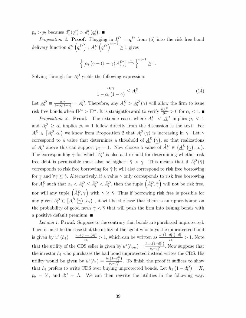
pg > pb because dg1 (qg0) > db1(qb0).

Proposition 2. Proof. Plugging in If∗i = qf∗i from (6) into the risk free bond

delivery function dDi

(qf∗i

): ADi

(qf∗i

)αi−1

≥ 1 gives

{[αi(γ + (1− γ)ADi

)] 11−αi

}αi−1

≥ 1.

Solving through for ADi yields the following expression:

αiγ

1− αi (1− γ)≤ ADi . (14)

Let ADi ≡αiγ

1−αi(1−γ)= ADi . Therefore, any ADi > ADi (γ) will allow the firm to issue

risk free bonds when Πf∗ > Πρ∗. It is straightforward to verify∂ADi∂γ

> 0 for αi < 1.

Proposition 3. Proof. The extreme cases where ADi < ADi implies pi < 1

and ADi ≥ αi implies pi = 1 follow directly from the discussion is the text. For

ADi ∈[ADi , αi

)we know from Proposition 2 that ADi (γ) is increasing in γ. Let γ

correspond to a value that determines a threshold of ADi(γ), so that realizations

of ADi above this can support pi = 1. Now choose a value of ADi ∈(ADi(γ), αi).

The corresponding γ for which ADi is also a threshold for determining whether risk

free debt is permissible must also be higher: γ > γ. This means that if ADi (γ)

corresponds to risk free borrowing for γ it will also correspond to risk free borrowing

for γ and ∀γ ≤ γ. Alternatively, if a value γ only corresponds to risk free borrowing

for ADi such that αi < ADi ≤ ADi < ADi , then the tuple(ADi , γ

)will not be risk free,

nor will any tuple(ADi , γ

)with γ ≥ γ. Thus if borrowing risk free is possible for

any given ADi ∈[ADi(γ), αi), it will be the case that there is an upper-bound on

the probability of good news γ < γ that will push the firm into issuing bonds with

a positive default premium.

Lemma 1. Proof. Suppose to the contrary that bonds are purchased unprotected.

Then it must be the case that the utility of the agent who buys the unprotected bond

is given by ub (h1) =h1+(1−h1)dDb

pb> 1, which can be written as

h1(1−dDb )+dDbpb

> 1. Note

that the utility of the CDS seller is given by us(hcds) =hcds(1−dDb )pb−dDb

. Now suppose that

the investor h1 who purchases the bad bond unprotected instead writes the CDS. His

utility would be given by us(h1) =h1(1−dDb )pb−dDb

. To finish the proof it suffices to show

that h1 prefers to write CDS over buying unprotected bonds. Let h1

(1− dDb

)= X,

pb = Y , and dDb = Λ. We can then rewrite the utilities in the following way:

39

ub (h1) = X+ΛY

and us(h1) = XY+Λ

. If us(h1) > ub (h1) then,

=⇒ X + Λ

Y<

X

Y − Λ=⇒ (X + Λ) (Y − Λ) < XY.

=⇒ −XΛ + ΛY − Λ2 < 0

=⇒ (X − Y + Λ) > 0.

Substituting back in for X, Y , and Λ we see that h1

(1− dDb

)− pb + dDb > 0, which

is the same ash1+(1−h1)dDb

pb> 1. Thus, any agent who would buy unprotected bonds

would be better off selling CDS.

Proposition 4. Proof. This follows directly from Che & Sethi (2014) with two

differences. 1) the marginal investor indifferent between selling CDS and having

exposure to another risky asset does not directly price the bond for which the CDS

is sold. The investor prices the return to the CDS relative to the return on the

alternative risky asset. 2) investment is endogenous so that supply of bonds qi is not

fixed.

Suppose to the contrary that pi ≤ pi, i = G,B, where pi is firm is bond price in

an economy with covered CDS and pi is the bond price in a Baseline Economy. The

expected return any given investor h places on selling a CDS is given by

h(1− dDi

)pi − dDi

.

In the up state, a CDS seller retains the value of the contract,(1− dDi

). The CDS

seller must hold enough collateral to sell this contact. That collateral value is equal

to 1 − dDi − pci . The fundamental recovery value of the bond dDi is not insured, and

investors receive a price for selling CDS that they can use as collateral for additional

contracts pci . This is a decreasing function of bond prices because higher bond prices

mean lower CDS prices. Higher bond prices mean investors need to post more of

their own cash as collateral to sell a CDS, which lowers the expected return to their

collateral. Thus, as bond prices decrease, the marginal investor indifferent to selling

a CDS and buying an alternative risky asset is less optimistic because the returns

to selling a CDS are increasing relative to the return on holding the alternative

asset. Therefore, h1 (pi (qi) , dsi ) ≤ h1 (pi (qi) , d

si ). The market clearing conditions in

the Baseline Economy and Covered CDS Economy for the firm for whom CDS are

40

written are, respectively, given by

1− h1 (pi (qi) , dsi ) = piqi (15)

1− h1 (pi (qi) , dsi ) = piqi − qidsi . (16)

Note that bond quantities are different across economies as well. However, it can be

shown that qi = βi × (pi)−Γi where βi ≡

(1αi

) 1αi−1

and Γi ≡ αiαi−1

< 0. This means

that ∂qi∂pi

> 0 and pi and qi move in the same direction. Thus the left hand side of

(16) is weakly greater than that of (15) while the right hand side is strictly less. A

contradiction. Hence pi > pi, i = G,B.

Corollary 1. Proof. This follows directly from Proposition 4 in that

h1(pB (qB) , dDB

)> h1

(pB (qB) , dDB

)where the tilde corresponds to bond pricing in

the Covered Economy and the hat corresponds to bond pricing in the Non-CDS

economy. The higher is the bond price, the lower is the CDS premium, which lowers

the return to “buying the Arrow-Up.” The resulting marginal CDS seller in the

Covered CDS Economy must therefore be more optimistic than the marginal bond

buyer in the non-CDS economy. Because the set of agents is connected, the next

most optimistic agent h1− in the covered CDS economy will be more optimistic than

h1− in the non-CDS economy.

Proposition 5. Proof. From Proposition 3 we know that if risk free borrowing

exists in the range of ADi for which pi = 1 is possible, it will only occur if γ is

below the threshold γ < γ < 1. From Proposition 4, we know that ∂qi∂pi

> 0 so that

qρ∗i > qρ∗i , bond quantities rise in the covered CDS economy. This therefore implies

that γqρ∗i > γqρ∗i = qf∗i . Lastly, we know that for the same ADi from the(γ, ADi

)-tuple

that made the two debt contracts equivalent in the Non-CDS economy, if issuing risk

free is chose in the covered CDS economy, there must be another γ < γ for which

the two debt contracts yield the same profits; otherwise, the firm always issues risky

debt in which case default always occurs at ADi .

Lemma 2: Proof. Suppose to the contrary that h1 holds cash. It must be the

case then that the investor prefers holding cash to any other instrument int the

economy. Thus we can say

h1 + (1− h1) dDb < pb, (17)

41

and

1 >(1− h1)

(1− dDb

)1− pb

. (18)

Inserting (17) into the denominator of the r.h.s of (18) we do not perturb the in-

equality

1 >(1− h1)

(1− dDb

)1− [h1 + (1− h1) dDb ]

.

Rearranging and regrouping we get

(1− h1)(1− dDb

)> (1− h1)

(1− dDb

)⊗

a contradiction.

Proposition 6. Proof. To see this consider the re-written equilibrium market

clearing condition for firm i when naked CDS are permitted where dots above vari-

ables indicate the naked CDS values:

1− h1(pi (qi) , d

Di

)= piqi − qidDi +

(pi − dDi

) h2

1− pi. (19)

The only functional form difference between (19) and (16) is the final term on the

right hand side,(pi − dDi

)h2

1−pi . This term is always greater than zero because pi >

dDi whenever a funding equilibrium exists. The left hand sides are the same form.

Consider to the contrary that pi ≥ pi in which case the left hand side of (19) is

less than or equal to the left hand side of (15). The right hand side of (19) is a

monotonically decreasing function of dDi . Suppose the upper-limiting case dDi = pi.

Then the right hand side of (19) is equal to zero and h1(pi (qi) , d

Di

)= 1 meaning

there is no equilibrium funding for firm i. Suppose the lower-limiting case where

dDi = 0, in which case the right hand side of (19) is strictly greater than that of (15),

a contradiction. Thus pi < pi for ∀dDi ∈[0, pDi

).

Proposition 7. Proof. The logic is the same as Proposition 5. Use qρ∗i < qρ∗i from

Proposition 6 and ∂qi∂pi

> 0 from Proposition 3.

C Retail Investor

Let his utility be given by UM (xs, cs) ε, ε > 0, where xs is time 1 consumption and

ci is a covered CDS package made up of a bond and CDS: ci = qi + qic.16 Since he

16The micro-foundations of the investor’s preferences are not explicitly modeled, though it is easyto do so. For example, one could assume the investor is a fund manager who invests in covered

42

holds no risk, a CDS contract will accompany every bond purchased. Furthermore,

UM ′ (ci) > 0 so that the investor always prefers to invest when the opportunity exists.

We can now characterize the institutional investor’s budget set:

BM (pi, pic) ={(xM0 , q

Mi , q

Mic , x

Ms

)∈ R+ ×R+ ×R+ ×R+ :

xM0 +∑i

(pi + pic) cMi = eM ,

xMs = xM0 +∑i

cMi

}.

The investor uses his endowment to either purchase bonds with covered CDS or

for consumption. The retail investor consumes the same amount in either state since

covered CDS positions have identical payouts in both states. Final consumption is

the sum of cash carried forward and the number of covered CDS packages purchased.

CDS for which he receives a fee given by ε.

43

Credit Default Swaps and Debt Contracts: Spillovers and ... · Credit Default Swaps and Debt...

Documents

Transcript of Credit Default Swaps and Debt Contracts: Spillovers and ... · Credit Default Swaps and Debt...