1

Creation of a digital flowline network from IfSAR 5-m DEMs

for the Matanuska-Susitna Basins: a resource for update of the

National Hydrographic Dataset in Alaska

By:

Dan Miller PhD, TerrainWorks Inc.

Lee Benda PhD, TerrainWorks Inc.

James DePasquale, The Nature Conservancy

David Albert, The Nature Conservancy

July 2015

2

CREATION OF A DIGITAL FLOWLINE NETWORK FROM IFSAR 5-M DEMS FOR THE MATANUSKA-

SUSITNA BASINS: A RESOURCE FOR UPDATE OF THE NATIONAL HYDROGRAPHIC DATASET IN ALASKA

Dan Miller, Terrainworks Inc., Seattle WA

Lee Benda, Terrainworks Inc., Shasta CA

James DePasquale, The Nature Conservancy, Anchorage AK

David Albert, The Nature Conservancy, Juneau AK

Abstract: High-resolution (5-m) elevation data available through the Alaska Statewide Digital

Mapping Initiative’s collection of interferometric synthetic aperture radar (IfSAR) digital

elevation models (DEMs) can be used to create digital representations of basin hydrography.

Here we explore the potential to use these IfSAR DEMs, with other available data sources, to

create digital hydrography with sufficient accuracy and completeness to update the National

Hydrographic Dataset (NHD) for Alaska. Efforts to create elevation-derived digital hydrography

using standard GIS processing tools available in ESRI’s ArcGIS have had limited success in

deriving accurate and complete channel networks, so for this project we augmented tools

available in ArcGIS with a suite of open-source programs developed through research and

extensive applied use in the Pacific Northwest. We have developed methods to merge disparate

elevation data sources into contiguous DEMs with minimal artifacts at seams, to utilize the open-

water breaklines derived from the IfSAR (and LiDAR) orthorectified intensity imagery to guide

flow paths through areas where topographic relief is insufficient to resolve channel courses, to

calibrate channel initiation criteria to local conditions, to obtain optimal flow paths that preserve

all topographic information when creating hydrologically conditioned DEMs, to breach road

crossings, and to smooth DEM-derived channel courses to provide improved estimates of

channel length and gradient. We have also worked to find efficient channels for feedback from

stakeholders and people familiar with basin hydrography to ensure that derived products are

accurate and can meet their needs. We describe these methods here, provide time estimates for

performing needed tasks, and discuss remaining issues.

3

Contents

Introduction .............................................................................................................. 5

NHD and NHDplus ................................................................................................................... 5

Methods. Digital Hydrography ............................................................................... 6

Merging DEMs. ......................................................................................................................... 8

Topographic attributes ............................................................................................................. 9

Drainage enforcement ............................................................................................................. 10

Water mask............................................................................................................................ 10

“Burning in” of known channel courses ............................................................................. 11

Road crossings ...................................................................................................................... 11

Known channel initiation points .......................................................................................... 11

Hydrologic conditioning ......................................................................................................... 11

Flow direction and flow accumulation .................................................................................. 13

Channel Initiation ................................................................................................................... 14

Slope-area product ................................................................................................................ 14

Plan curvature and minimum flow length ........................................................................... 15

Spatial variability .................................................................................................................. 15

Smoothing of channel traces................................................................................................... 15

Channel networks as sets of linked nodes ............................................................................. 15

Results for the Matanuska-Susitna ......................................................................16

Merged DEMs .......................................................................................................................... 16

Topographic attributes ........................................................................................................... 18

Drainage enforcement ............................................................................................................. 19

Water mask from IfSAR and LiDAR breaklines ................................................................. 19

Surveyed channels ................................................................................................................ 20

Known channel initiation points .......................................................................................... 21

Road crossings ...................................................................................................................... 22

Hydrologic conditioning ......................................................................................................... 23

Channel initiation .................................................................................................................... 24

Slope-area product ................................................................................................................ 24

Plan curvature and minimum flow length ........................................................................... 24

4

Channel course smoothing...................................................................................................... 25

Remaining tasks ...................................................................................................................... 26

Validation .............................................................................................................................. 26

NHD flowline endpoints and type ........................................................................................ 26

Lakes ..................................................................................................................................... 27

Downstream branching ........................................................................................................ 27

Catchment polygons.............................................................................................................. 27

Shoreline ............................................................................................................................... 27

Hardware and software requirements .................................................................28

Time requirements .................................................................................................................. 28

Next steps ................................................................................................................30

Creation of NHDplus datasets ................................................................................................ 30

Compatibility with modeling and decision support tools .................................................... 30

Data attributes for created flowline networks ...................................................................... 31

Citations ..................................................................................................................31

5

Introduction Through the Statewide Digital Mapping Initiative’s collection of interferometric synthetic

aperture radar (IfSAR), Alaska now has data resources to develop a high-resolution, GIS-based

hydrographic dataset that fully integrates land-surface and channel-network features. The IfSAR

data provide a unique opportunity for updating the Alaska Hydrography Database (AK Hydro),

and thereby the National Hydrography Dataset (NHD), and for creation of high-resolution

NHDplus datasets. Here we describe our efforts to use these data to create accurate and complete

high-resolution hydrography for the Matanuska-Susitna Basins.

NHD and NHDplus

NHD provides a nation-wide GIS representation of surface-water features. With NHD, everyone

working with hydrographic data can use a common GIS topology, can document their work

using the same formatting and metadata standards, and – most importantly – everyone working

in the same geographic area can start with the same flowline, water body, and watershed

boundary geometries. NHD provides consistency so that users can distribute monitoring and

survey data, can share analysis tools and modeling results, and can communicate with a common

vocabulary.

NHDplus expands on the capabilities of NHD by linking land areas to NHD flow lines. These

linkages are established using Digital Elevation Models (DEMs) from the National Elevation

Dataset (NED). With information about the land-surface characteristics that affect stream flow

linked directly to the channels, NHDplus provides modeled estimates for channel attributes, such

as discharge and flow velocity.

The NHD and NHDplus are incredibly valuable resources. However, NHD data for Alaska are

incomplete, outdated, of low resolution, and often inaccurate, which hinders adaption of NHD as

a single-source hydrography dataset. A variety of efforts are underway to update NHD features

in Alaska, with participants in AK Hydro coordinating these efforts and working to synchronize

updated water-feature geometries to the NHD (see the AK Hydro Manual).

Updates to mapped surface water features are typically based on interpretation of new imagery

and from geo-referenced field surveys. The IfSAR data offer a substantial complement to these

methods for broad-scale hydrologic mapping. IfSAR 5-m DEMs are of sufficiently high

resolution to accurately delineate entire channel networks, complete through headwaters that

experience seasonal or ephemeral flow. Additionally, the orthorectified radar intensity images

(ORIs, with 2.5-m resolution) show areas of open water, from which two-dimension geometry

for the complex, anastomosing channel systems common to glacial river systems can be

demarcated and used to guide channel placement.

Creation of digital hydrography based on flow paths inferred from digital elevations provides

substantial benefits over hydrography created from other sources, such as heads-up digitizing

from optical and shaded relief imagery, because channel flowlines are explicitly linked to a

digital representation of the land surface. Flow routing across the landscape and delineation of

watershed boundaries or catchments can be done consistently and unambiguously directly from

DEM flow paths, with no additional processing of the DEM. This explicit linkage of the

6

hydrography to the DEM greatly simplifies use of these data in creation of NHDplus datasets and

for using hydrologic, geomorphic, habitat, and hazard assessment models.

Our goal is to use the newly available IfSAR data to build accurate digital hydrography. Here we

describe a test case with our work in the Matanuska-Susitna basins. IfSAR DEMs and ORIs,

supplemented with LiDAR data where it was available, were used to generate a complete, basin-

wide flow-line network of consistent resolution and accuracy. The area involved exceeded

63,000 square kilometers and over 145,000 kilometers of channels were included in the traced

network. Channel locations and upstream extent are being validated using aerial imagery and

field surveys, and the digital hydrography will be corrected where errors or omissions are found.

Preliminary results indicate that the DEM-traced network is highly accurate, following channel

courses precisely, and that errors in flow-line location are generally obvious, occurring where

topographic indications of channels become indistinct or disappear, as when all flow goes

subsurface in deep glacial outwash sediments.

Methods. Digital Hydrography There are few examples using elevation-derived digital hydrography to update NHD flowlines to

serve as a guide (Poppenga et al., 2013), and efforts using traditional spatial analysis tools (i.e.,

ESRI ArcGIS Hydrological Tools) “proved to be difficult and time consuming” (Kaiser et al.,

2010). Given the benefits provided by a digital representation of basin hydrography that is fully

integrated with a digital representation of the landscape it drains, and the opportunities offered

by the high-resolution IfSAR data for Alaska of realizing that potential, we therefore seek

alternatives that can make the job easier and faster.

Our tactic is to provide an initial flowline network that is accurate and complete, which will

simplify validation, and that is updatable as new data become available or channel courses

change. We also want to ensure that the data files created can be used to explicitly link all parts

of the terrestrial-river system to facilitate creation of NHDplus datasets and provide input files

for models that use NHDplus or depend on flow routing through a DEM. Additionally, we want

to provide data formats that enable use and development of a broad range of models for

geomorphic and hydrologic processes, and that will work with all Geographic Information

Systems.

The data structures, methods, and algorithms we have found that work best for building accurate

and complete digital hydrography have grown out of programming used to explore temporal and

spatial patterns of landscape dynamics (Benda and Dunne, 1997a, b; Benda et al., 1998; USDA

Forest Service, 2003) and from use of these programs for applied analyses (Benda et al., 2007),

including creating digital hydrography from DEMs (Agrawal et al., 2005; Bruno et al., 2014;

Busch et al., 2011; Clarke et al., 2008; Flitcroft et al., 2014; McCleary et al., 2011; Peñas et al.,

2014; Sheer and Steel, 2006; Steel et al., 2004; Steel et al., 2008), assessing aquatic habitat

potential (Bidlack et al., 2014; Burnett et al., 2007), delineating floodplains (Benda et al., 2011)

and riparian zones (Fernández et al., 2012b), mapping of landslide hazards (Burnett and Miller,

2007; Hofmeister and Miller, 2003; Hofmeister et al., 2002; Miller and Burnett, 2008), and

assessing potential for wood recruitment to streams (Atha, 2013; Benda et al., 2003). These

methods have evolved and continue to grow through extensive, collaborative use, and they have

7

demonstrated superior performance in comparisons with other options for extraction of channel

networks (Peñas et al., 2011) and riparian zones (Fernández et al., 2012a) using DEMs.

Numerical analyses used for these methods are implemented in a set of Fortran programs

referenced as Netstream (Miller, 2003), licensed under the GNU General Public License v3

(GPLv3). We use Fortran because the current language standard (Fortran 2008, http://www.j3-

fortran.org/) implements usage and protocols for numerical analysis of very large datasets,

current Fortran compilers provide options for fully optimized, vector and parallel processing on

current CPUs, and Fortran libraries are interchangeable with C-language libraries. The programs

operate using command-line interfaces and, as demonstrated by the citations above, are available

for anyone to use and modify. The programs have been incorporated into a user interface for

ArcGIS using vb.net and python scripts (Benda et al., 2007).

In this section, we describe the methods and algorithms used to create a synthetic channel

network using the LiDAR, IfSAR, and NED elevation data available for the Matanuska-Susitna

basins. This involved nine primary tasks:

1. Merge available elevation data to a single, contiguous DEM for the entire

watershed. IfSAR 5-m DEMs were available for most, but not quite all of the area, and

1-m LiDAR bare-earth DEMs were available for a portion of the area. We wanted to

maintain information from the most precise and accurate data in creation of a single,

contiguous DEM, while also avoiding creation of breaks in elevation or derivatives of

elevation (gradient, curvature) at seams between the different data sources.

2. Calculate topographic attributes used for network extraction. We want to base these

values on unaltered elevation data, prior to drainage enforcement and hydrologic

conditioning. The attributes we need are surface gradient, plan curvature, and the contour

length crossed by flow out of a DEM cell, which is used to calculate specific contributing

area. In this step, we must choose an appropriate length scale over which these attributes

are calculated. This length scale typically spans several DEM cell lengths.

3. Identify data sets to use for drainage enforcement. We have four sources of

information with which to guide flow directions and specify channel initiation locations:

a) polygons of open water digitized from imagery of reflected intensity for the LiDAR

and IfSAR data; flow lines should run down the center of these polygons, b) GIS vector

line files of channel centerlines from accurate field surveys, c) line segments indicating

culvert locations at road stream crossings, and d) points of known channel initiation.

4. Create a hydrologically conditioned DEM, for which flow paths out of all closed

depressions are identified. We use a combination of depression filling (Jenson and

Domingue, 1988) and carving (Soille et al., 2003).

5. Calibrate channel-initiation criteria. We use criteria based on flow accumulation and

surface slope, plan (contour) curvature, and flow length over which these criteria are met.

Our goal is to set criteria, which may vary spatially, to identify all channels that can be

resolved with the elevation data.

6. Calculate flow accumulation, identify all channel initiation points, and trace all

channels. We apply the D-infinity algorithm (Tarboton, 1997) to calculate flow

8

accumulation values used to identify channel initiation points. Channels are then traced

downstream from these points using D-8 flow directions (Jenson and Domingue, 1988) to

preclude dispersion of channelized flow. D-8 flow directions are chosen using a

combination of steepest descent and largest plan curvature (Clarke et al., 2008).

7. Smooth channel traces to provide better-placed channel centerlines and more accurate

estimates of channel length and gradient.

8. Validate the delineated channel network using a combination of local knowledge, field

surveys, and high-resolution optical imagery. Check channel locations, channel extent,

road diversions, and delineation of water bodies.

9. Update all datasets and adjust channel initiation criteria based on errors identified in

Step 8 to correct flow directions and adjust channel initiation criteria. Iterate Steps 5

through 8 until all specifications for accuracy and completeness are met.

We have worked through all of these steps using a subset of the project area, referred to here as

the core area. That exercise helped us to choose algorithms, make modifications to programs

used for analyses, and calibrate channel initiation criteria to use for the entire basin. Validation

of the draft flow-line network for the entire basin is now being done by GeoSpatial Services at

Saint Mary’s University of Minnesota. After needed corrections to the flow lines are identified,

they will be used to construct a final fully routed and attributed flow-line network with

accompanying raster files.

Merging DEMs.

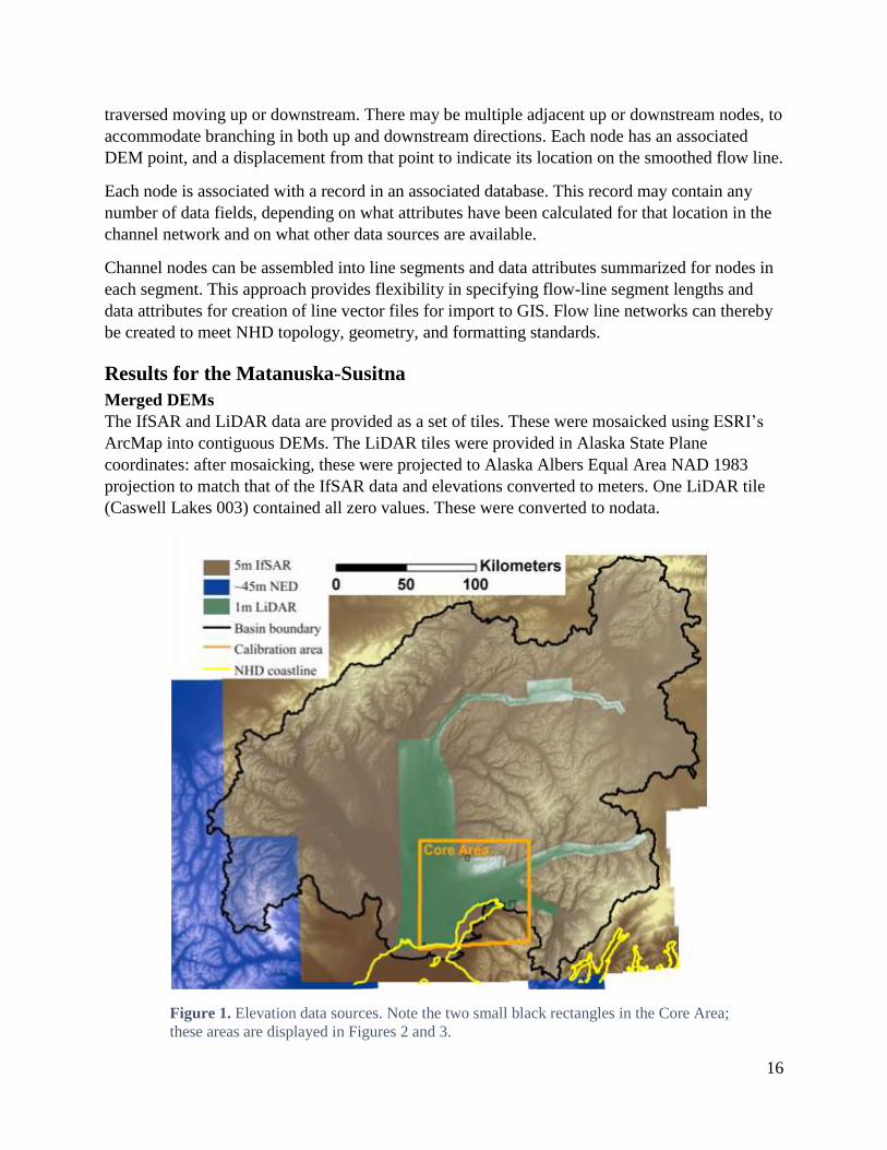
We lacked a single high-resolution DEM for the entire Matanuska-Susitna watersheds. We had

1-m LiDAR bare-earth DEMs for a portion of the area, a 5-m IfSAR DEM for almost the entire

area, and the 3-arc second NED DEM for the entire area. The areas of the basin covered by each

data source are shown in Figure 1.

Our strategy to combine these three data sources into a single, contiguous DEM was to use the

highest-resolution data where it existed, and to smoothly merge it onto the low-resolution data

over a user-specified transition length. Within this transition zone, the average elevation of the

merged DEM, calculated over a user-specified radius, transitions linearly from that of the high-

resolution data to that of the low-resolution data, with the topographic detail of the high-

resolution data maintained.

The average elevation of the low- and high-resolution data may differ by amounts large enough

to significantly alter estimated channel gradients. To determine an appropriate transition length,

we examine the magnitude of the elevation differences between the two data sets and set a

transition length sufficiently long enough to cause no changes in gradient larger than some

chosen limit.

Within the transition zone, the average elevation of an output DEM point is calculated as a linear

function of the average elevations of the low- and high-resolution DEMs:

�̅� = �̅�𝐿𝑟 + �̅�𝐻(1 − 𝑟)

9

where �̅� is the average elevation of the output DEM, �̅�𝐿 is the average elevation of the low-

resolution DEM, �̅�𝐻 is the average for the high-resolution DEM, and r is a value varying from

zero to one and indicates the proportion of the transition distance the output DEM point is from

the closest edge of the high-resolution DEM. Thus, at the edge of the high-resolution DEM, the

output DEM has an average elevation equal to that of the low-resolution DEM. At the edge of

the transition zone inside of the high-resolution DEM, the output DEM has an average elevation

equal to that of the high-resolution DEM. Within the transition zone, the average elevation of the

output DEM varies linearly between the averages of the low- and high-resolution data.

The elevation at a point is taken as the average elevation of the merged DEMs plus the difference

between the average and actual high-resolution data at that point. This way, we obtain a smooth

transition between the two DEMs, while maintaining the detail of the high-resolution data.

We also define a second merge length, which provides a smooth transition from the high-

resolution detail to the low-resolution detail near the edge of the high-resolution DEM in the

transition zone. Within the merge zone, the elevation added to the average varies from the

difference between the average and actual elevations from the high-resolution data to that from

the low-resolution data. This prevents breaks in the elevation profile created where features

resolved in the high-resolution DEM are not seen in the low-resolution DEM. This merge length

can be much shorter than the transition length. Good results are typically obtained if it spans 5 or

more output-DEM cells.

The output DEM has a user-specified point spacing and corner location. These do not need to

match those of either input DEM. Elevation values from the original DEMs are obtained using

bilinear interpolation.

Topographic attributes

Gradient and curvature at each DEM point are calculated by fitting a partial quartic equation to

elevations at the point and eight surrounding points, as described by Zevenbergen and Thorne

(1987). The 8 surrounding points are located on a circle centered at the DEM point, as described

by Shi et al. (2007). Radius of the circle determines the spatial grain at which gradient and

curvature are estimated. The smallest length scale over which these values can be resolved is

twice the grid spacing of the DEM. Elevation at points on the circle that do not fall directly on a

DEM grid point are determined using bilinear interpolation.

Using the partial quartic solution of Zevenbergen and Thorne (1987), gradient requires elevation

values only along the cardinal directions (e.g., N-S and E-W). To reduce bias from the

orientation of the DEM grid, gradient is calculated twice, first using elevations along the cardinal

DEM orientation, and then again at an orientation rotated 45 degrees. Gradient at the point is

determined as the average of the two values (the modified Zevenbergen -Thorne method of Shi

et al., 2007).

To estimate specific contributing area (contributing area per unit contour length) for each DEM

cell, we need the contour length crossed by flow exiting each cell. Ideally, this contour length is

estimated by integrating the projection of flow direction (for outgoing flow only) over a circle

centered at the DEM point, with the circle radius the same as that used for calculating gradient

10

and curvature. For length scales spanning several DEM grid cells, however, this method proved

rather slow. As an alternative, we used the surface representation applied for the D-infinity flow-

direction algorithm (Tarboton, 1997): that of eight triangular facets defined for a cell centered

over the grid point, with edge length equal to the specified length scale, and with corner

elevations obtained with bilinear interpolation. The projection of flow direction out of each facet

is then integrated along each facet edge and summed over all facets. For planar flow, this gives a

contour length of one cell length. For divergent flow, the contour length is greater than the cell

length, and for convergent flow, it is less. Specific contributing area is then obtained by dividing

the flow accumulation calculated for a DEM cell (using D-infinity) by the contour length crossed

by flow exiting the cell, both normalized by cell length.

The appropriate length scale to use for calculating topographic attributes depends on the ability

of the DEM to resolve surface features, on the amount of noise in the DEM (which can create

spurious high curvature values), and on the spatial scale of the topography controlling the

physical processes being modeled (e.g., Pirotti and Tarolli, 2010).

Note that these topographic attributes are all calculated for the original DEM, not the

hydrologically conditioned DEM. Our intent is to base analyses on data that has been altered as

little as possible.

Drainage enforcement

We use four sources of information to guide flow directions and to augment automated methods

for identifying points of channel initiation: 1) A water mask, which consists of polygons

delineated from remotely sensed open water in channels. Elevations within a water mask are set

to be monotonically decreasing downstream and to direct flow towards the center of the mask. 2)

Vector lines defined from high-accuracy and high-resolution field surveys, along which a swale

of specified width and depth is excavated (burned in), 3) vector line segments indicating culvert

locations at road stream crossings, and 4) channel initiation points, located from high-resolution

aerial photography or field surveys.

Channel initiation is allowed within water masks, on vector channels, and on mapped initiation

points, even if all criteria for topographically determined channel initiation are not met.

Water mask

If other data sources can be used to delineate areas of open water in surface channels, these can

be used to guide flow directions (Burnett et al., 2013). This is particularly useful in areas of low

relief where topographic indicators of channels may be ambiguous. With LiDAR and IfSAR

data, areas of open water have no returns, so a “water mask” can be created from areas with no

reflectance. For this project, the contractors providing the LiDAR and IfSAR DEMs also

provided vector breaklines delineating zones of open water digitized from areas with no (zero

intensity) returns. Elevations within these known locations of open water had been “hydro

flattened” in the DEM, following guidelines specified in Heidemann (2014), so that elevations

within the channel polygons were, for the most part, constant across the channel, perpendicular

to the flow direction, and decreased in a downstream direction.

11

Because the DEM had already been hydro-flattened within the delineated water mask polygons,

we limited further processing solely to direct flow towards the center of each polygon; that is,

along the channel centerline. To direct flow towards the center, we delineate the skeleton of each

polygon by mapping local extremes (ridges) in a map of minimum Euclidean distance from the

polygon edge (e.g., Chang, 2007). We then lowered elevations along the delineated centerline

skeletons.

“Burning in” of known channel courses

Drainage enforcement along known channel courses is done by excavating a swale in the DEM,

centered over the vector lines that represent the channel centerline. The depth and width of the

excavated swale are adjustable to provide more or less enforcement of flow directions.

Road crossings

A swale is also excavated into the DEM at specified culvert locations. The depth of the swale is

set by the elevations found at both ends of a line segment crossing the road prism. Width of the

swale is a user-specified parameter.

Known channel initiation points

Within wetland complexes and areas of shallow groundwater upwelling, channelized surface

water can appear in areas with very little contributing area (based on surface topography) and

with no topographic convergence (low or zero plan curvature). These locations cannot be

identified using topographically defined criteria for channel initiation. To include these channels,

we rely on other data. These types of channels may be visible in the high-resolution optical

imagery, for example.

Hydrologic conditioning

For each cell of the DEM, we seek to define a flow direction consistent with surface-water flow

paths. To create a “hydrologically conditioned” DEM, we also require that flow traced from

every cell eventually reaches an outlet from the DEM. This requires that a flow path out of all

closed depressions in the DEM be defined. Within a DEM, closed depressions occur for a variety

of reasons. When elevation data are of sufficient detail to resolve road surfaces, as with the

LiDAR bare-earth DEMs, road prisms at stream crossings can appear as dams blocking

downstream flow. Flow through culverts must be accounted for. Closed depressions may also

occur as artifacts due to noise in the DEM, or from unresolved low points. Topographic closed

depressions also exist on the ground surface, and for these we wish to find the flow path that

water would follow if the depression were to be filled and overtopped.

For identified road crossings, we digitize short line segments that span the road prism and reduce

DEM elevations along the line segment to allow drainage through the road prism, as described in

the previous section on drainage enforcement. Identification of road crossings is typically done

iteratively, as diverted flow paths are identified in traced channel networks.

For all other closed depressions, there are two approaches are used to define flow paths (Poggio

and Soille, 2012): incremental methods, where elevations within depressions are increased to the

elevation of the pour point (the point where water flows out of a depressions as it is overtopped),

and decremental methods, where elevations are reduced along some path to drain the depression.

12

Hydrologic conditioning of DEMs that use decremental methods are found to produce more

accurate channel courses (Poggio and Soille, 2012) and channel profiles (Byun and Seong,

2015). Our experience in the Matanuska-Susitna Basins is similar: we find that decremental

methods produce more accurate flow paths, particularly for very small channels. Incremental

methods tend to obscure topographic information within areas where elevations are increased to

drain depressions. With the IfSAR and LiDAR data, many minor depressions result because of

apparent noise in the elevation data. Topographic expression of small channels may span only a

few DEM cells; filling of small noise-generated depressions in some cases caused the D-8 flow

direction to diverge from the channel course, particularly for those with no water-mask

breaklines.

To define an optimal path along which to reduce elevations to drain a depression, we used D-8

flow directions and steepest descent from the pour point. On the depression side of the pour

point, this traces a path to a low point in the depression. If a flat zone is encountered along the

path, the method described by Garbrecht and Martz (1997), as modified by Barnes et al. (2014a),

is used to define flow directions through the flat zone. On the outlet side of the pour point, the

steepest descent path is followed until an elevation less than or equal to that of the low point in

the depression is encountered. Elevations along the paths emanating from the pour point, one

into the depression and one away from it, are then lowered to that of the low point in the

depression. This provides a flow path out of the depression along which flow directions are

defined. This method maintains flow direction information that is lost by depression filling.

Draining of the DEM, with identification of depressions and pour points, is initiated from low

points along the edge of the DEM, that is, from points where elevations indicate flow directed

out of the DEM. We use a queue to define an expanding wavefront from each of these flow

outlets. The wavefront expands outward cell-by-cell, extending into adjacent cells with

elevations greater than or equal to that of the cells already on the wavefront. Because the

wavefront expands only to cells at equal or higher elevations, all cells crossed by the wave front

have flow paths to an outlet.

At some point, the wavefront can expand no more without extending into cells with lower

elevations. The edge of the wavefront is then traversed and low points along the edge are

identified – these are pour points for undrained depressions. The pour points are ordered by

elevation, from lowest to highest, using a priority queue, and the depressions are drained starting

with the lowest-elevation pour point. Each time a flow path out of a depression is defined, the

wavefront expands to encompass all drainable cells, new pour points are identified, and the

priority queue of pour points is updated. This process continues until all cells in the DEM are

drained.

This procedure is not as computationally efficient as the flood-fill algorithms described

elsewhere (e.g., Barnes et al., 2014b), but it works well for maintaining channel courses when

breaching large barriers, such as unidentified road prisms and dams, and for finding optimal

paths through flat areas encountered while identifying flow from pour points to a low point in a

depression.

13

Flow direction and flow accumulation

Once the DEM has been hydrologically conditioned as described above, all cells have an

adjacent cell of equal or lower elevation. For cells with an adjacent cell of lower elevation, the

D-infinity method (Tarboton, 1997) is used to define the primary direction of flow out of the cell.

D-infinity is one of a family of flow-direction algorithms that can account for dispersion of flow

over divergent topography by proportioning flow out of one cell into more than one downslope

cell, unlike the D-8 algorithm, which sends all flow into one of the eight adjacent cells (Wilson

et al., 2008). D-infinity limits the amount of dispersion by allowing flow into no more than two

downslope cells. It is computationally efficient and is found to provide estimates of flow

accumulation considerably more accurate than D-8 (Wilson et al., 2007) and of comparable

accuracy as other dispersive algorithms for mathematically constructed surfaces with known

contributing area (Qin et al., 2013) and to also perform well for prediction of field-observed soil

wetness (Sorensen et al., 2006).

Cells surrounded by areas of equal or higher elevation form flat areas within the DEM, for which

flow directions are undetermined. To define flow directions through flat zones, we use the

algorithm described by Garbrecht and Martz (1997), as modified by Barnes et al., (2014a). This

algorithm directs flow away from higher terrain and towards lower terrain; this produces flow

paths that tend to traverse through the center-line of flat zones.

After flow directions are defined for all DEM cells, flow accumulation to each cell is calculated

using the iterative approach described by Tarboton (1997). Initially, prior to calibration of

channel initiation criteria, D-infinity flow directions are used for all cells. We use the resulting

flow accumulation values to estimate optimal values for the slope-area thresholds used for

channel initiation, as described below. Once thresholds for the slope-area product, plan

curvature, and minimum flow length are set, flow accumulation is again calculated, but this time,

D-8 flow directions are used once the criteria for channel initiation are met. This prevents

dispersion of channelized flow.

To determine the D-8 flow direction for a cell, the method of steepest descent is commonly used,

in which flow is directed to the adjacent cell for which the downhill slope (calculated as the

elevation difference between DEM points divided by the distance between DEM points) is

greatest. We have found, however, that in areas with relatively planar slopes, small channel

courses are not well traced with this method, particularly if the channel does not align with one

of the D-8 directions. We find that small channels are better traced using a combination of

steepest descent and largest plan curvature. Use of plan curvature is similar to use of contour

crenulations to trace channel courses (Strahler, 1957); we want to direct channel flow both

downslope and along the course with topographic characteristics most indicative of a channel.

To choose the appropriate D-8 direction for channelized flow from a cell, we use the D-infinity

method of proportioning flow between downslope cells. If any adjacent cell receives more than a

greater proportion of flow (e.g., 75%), as estimated with D-infinity, then the D-8 flow direction

is set to that cell. However, if flow is more equally divided between two downslope cells, then

the D-8 flow direction is set to the cell with the largest plan curvature. The threshold proportion

of flow is a user-specified value, which we have set through trial and error to 75%.

14

It is also useful to define D-8 flow directions for all cells. Watershed boundaries and local

contributing areas to any point can be readily estimated by tracing D-8 flow paths until cells with

no inflow are encountered. D-8 flow directions are used, for example, to delineate catchments in

creation of NHDplus datasets. To translate D-infinity flow directions to D-8 flow directions, we

set the D-8 direction to the adjacent downslope cell that receives the majority of flow (as

estimated using D-infinity). Again, if flow is partitioned equally between two cells, the one with

the greatest plan curvature is chosen, and if both cells also have the same plan curvature, the one

along a cardinal direction is chosen.

In certain cases, D-8 flow directions, whether determined using the methods described here or

based solely on steepest descent, result in a flow direction diagonally across a DEM cell that

crosses a traced channel traversing the cell along the other diagonal. Then, if the D-8 flow

directions are used to delineate the local contributing area to one side of a channel segment, it

will appear as though drainage from both sides is flowing into the channel from only one bank.

After channel courses are traced, we check for this condition and redirect channel-crossing flow

into the channel.

Channel Initiation

Our goal is to calibrate criteria to identify channel initiation locations to delineate all channels

that can be resolved with the available elevation data. We use three criteria to identify channels:

1) a minimum value of the product ASe, where A is specific contributing area, S is surface

gradient, and e is a user-specified exponent, 2) a minimum plan curvature, and 3) a minimum

flow length along which the previous two criteria must be met.

Slope-area product

Given our goal of identifying all topographically defined channels, use of the area-slope product

is not necessary (e.g., Pelletier, 2013). We include it because, depending on the resolution and

precision of the DEM, not all small channels may be resolved, so that their presence must be

inferred. Inclusion of area and slope in the criteria for recognizing channels provides additional

controls on traced channel extent. This added control proves useful in landscapes where current

topography may be representative of past processes, such as meltwater and outburst flood

channels formed during past periods of glacial advance.

To identify appropriate thresholds for the area-slope product, we plot the channel density that

would result as a function of the ASe threshold. The inferred channel density decreases with

increasing ASe values, and on a log-log plot, in the vicinity of feasible channel densities (e.g., 1-

100 km/km2), we commonly find that channel density plots as a nearly straight line, but with an

inflection at some point, beyond which the rate in decrease of channel density with increasing

ASe values becomes smaller. This inflection point seems to indicate the AS

e value below which

“feathering” occurs, in which many small, parallel channels are traced up relatively planar slopes

(Montgomery and Foufoula-Georgiou, 1993). We use the location of this inflection point as a

guide in setting the area-slope product threshold for channel initiation.

15

Plan curvature and minimum flow length

Two aspects of plan curvature influence identification of channel initiation locations and

resulting channel density: the length scale over which curvature is calculated and the threshold

value below which channel initiation is precluded. We have not yet developed automated

methods to assist in choosing these values (e.g., Pelletier, 2013; Sofia et al., 2011), but we

recognize their importance in identifying channel extent, and so include explicit, though

subjective, methods for setting these values.

Thresholds for plan curvature and the minimum flow length over which these thresholds must be

met are set subjectively by plotting on shaded relief and optical imagery all the initiation points

identified under different ranges of values. Our goal is to set the plan curvature threshold as low

as possible without including non-channel features, such as tree wells (the holes formed by trees

that tip over, of which there can be many in forested areas), and noise in the DEM.

Spatial variability

We also recognize that a variety of channel-forming processes act across the landscape, and that

different processes may require different channel-initiation criteria. To address this, we allow the

initiation criteria to vary spatially. In concept, initiation criteria can then be calibrated for areas

with different soil types, for example. In practice, we have used separate initiation thresholds

based on surface gradient. We calibrate one set of values for steep terrain and another for low-

gradient terrain, based on the assumption that overland flow and landslide processes are the

primary channel-forming mechanisms in steep areas and seepage erosion the primary mechanism

in low-gradient areas (Dunne, 1980). Following Clarke et al. (2008), we calibrate channel

initiation thresholds for two zones: areas with surface gradient less than 25% and those with

surface gradients greater than 40%. The threshold values are varied linearly between these two

endpoints for areas with gradients in between.

Smoothing of channel traces

Flow lines defined by following D-8 flow directions consist of a series of straight-line segments

following DEM cell edges or diagonals. This gives flow lines a jagged appearance and results in

over-estimated channel lengths and under-estimated channel gradients. We therefore smooth the

traced channel courses by fitting a polynomial of specified order over a centered window along

the traced channel flow lines. The polynomial is over fitted, in that the window includes more

DEM points than needed to define the polynomial. This gives a smooth curve traversing points

within the window. This is done from each DEM point along the flow line and the vertex of the

flow line at that point is shifted to the location along the fit polynomial curve.

Channel networks as sets of linked nodes

We want to maintain information at the finest spatial grain available, with the ability to

summarize over any larger spatial scale. For the traced channel network, the finest spatial grain

is that of the DEM points that the flow lines follow. We therefore use a linked-node data

structure, which maintains information at this spatial scale.

Each DEM point along the traced flow lines defines one channel node. Each channel node is

connected to its adjacent upstream nodes and downstream nodes, so that the network can be

16

traversed moving up or downstream. There may be multiple adjacent up or downstream nodes, to

accommodate branching in both up and downstream directions. Each node has an associated

DEM point, and a displacement from that point to indicate its location on the smoothed flow line.

Each node is associated with a record in an associated database. This record may contain any

number of data fields, depending on what attributes have been calculated for that location in the

channel network and on what other data sources are available.

Channel nodes can be assembled into line segments and data attributes summarized for nodes in

each segment. This approach provides flexibility in specifying flow-line segment lengths and

data attributes for creation of line vector files for import to GIS. Flow line networks can thereby

be created to meet NHD topology, geometry, and formatting standards.

Results for the Matanuska-Susitna

Merged DEMs

The IfSAR and LiDAR data are provided as a set of tiles. These were mosaicked using ESRI’s

ArcMap into contiguous DEMs. The LiDAR tiles were provided in Alaska State Plane

coordinates: after mosaicking, these were projected to Alaska Albers Equal Area NAD 1983

projection to match that of the IfSAR data and elevations converted to meters. One LiDAR tile

(Caswell Lakes 003) contained all zero values. These were converted to nodata.

Figure 1. Elevation data sources. Note the two small black rectangles in the Core Area;

these areas are displayed in Figures 2 and 3.

17

The NED 3-arc-second tiles were also mosaicked and projected to Alaska Albers Equal Area

NAD 1983. After projection, the NED DEM had a horizontal point spacing of about 45 m.

These three DEMs were then exported to binary floating point format for import to the Fortran

program Merge, which we use to combine DEMs of differing resolution, as described in the

methods section. Floating point (flt) format is a non-proprietary file format that we have used for

importing and exporting raster data.

We first merged the 3-arc-second NED DEM with the 5-m IfSAR DEM at a horizontal posting

of 5 meters. This provided basin-wide elevation data. We then merged that DEM with the 1-m

bare-earth LiDAR DEM, and again posted elevations on a 5-m horizontal grid. This provided the

DEM used for all subsequent processing. We used a 5-m horizontal posting to maintain

consistency with the IfSAR data and to keep raster file sizes from becoming very large. With a 5-

m posting, the resulting ArcGIS raster for the Matanuska-Susitna basins requires about 14

Gbytes of disk space. A 1-m DEM would require about 25 times this amount (~350 Gbytes).

For each case, mean elevations were calculated over a radius of 150m. Merging was done over a

3000-m transition length, with a 100-m zone used to smooth topographic detail from the high to

low-resolution data. A shaded relief image showing an area at the seam between the LiDAR and

IfSAR DEMs is shown in Figure 2.

Figure 2. Comparison of IfSAR 5-m DEM and LiDAR 1-m DEM shaded relief, left panel,

and the merged DEM sampled at 5 m, right panel.

18

The LiDAR and IfSAR data both have areas within Cook Inlet and Knik Arm where elevations

values are all zero. There are also areas within channels draining to Cook Inlet with elevation

less than zero. We initially treated all elevation values of zero or less as nodata. This proved

unacceptable, however, because traced channels did not always extend to Cook Inlet.

Subsequently, we used the NED high-resolution flow lines, including only those classified as

“Coastline”, to define a shoreline. All elevation values landward of this shoreline, including

those of zero or less, were treated as legitimate elevation values and all areas ocean-ward of this

line set to nodata.

Topographic attributes

We experimented with a range of length scales for calculation of topographic attributes of

surface gradient, plan curvature, and contour length crossed by flow out of each DEM cell.

Figure 3 provides an example for plan curvature. A length of 25 meters (radius of 12.5m) proved

sufficient to smooth high-curvature values arising from smaller-scale variations in the DEM

elevations.

Figure 3. Plan curvature calculated over a 10-m length (left panel) and 50-m length (right panel).

19

Drainage enforcement

Water mask from IfSAR and LiDAR breaklines

Breaklines delineating open water were provided as polygons derived from the IfSAR radar

intensity imagery and from the LiDAR reflected intensity imagery (Figure 4). These breaklines

were digitized by the contractors providing these data. Breaklines from the LiDAR imagery had

been classified as Lakes, Single Line, and Double Line channels. Single-line channels had been

buffered to provide a polygon feature class. Breakline polygons from the IfSAR and LiDAR

imagery had been merged and were provided as a single polygon feature class.

All polygon features classified as “Lake” were filtered out and the remaining polygons used as a

water mask to guide flow directions for tracing channel courses. Breaklines from the IfSAR

imagery had not been classified, and many lake features therefore remained in the feature class.

We experimented with several methods to automatically delineate lakes from channels, such as

setting a threshold area to perimeter ratio, but did not find a satisfactory solution. This issue will

be revisited after review of the draft flow-line network. If an acceptable automatic solution

cannot be found, lake features in the IfSAR breaklines will need to be manually classified. This

classification is needed both to prevent channel initiation within lake features and so that flow

lines crossing lakes can be properly classified in the flow line network.

Neither IfSAR nor LiDAR (at the wavelength used for this project) provide elevation values over

open water. Water surface elevations within the breaklines must therefore be estimated from

values on the adjacent channel and lake boundaries (Heidemann, 2014); a process called hydro-

flattening. Noise in the elevation data, such as from reflections off vegetation, hinder

interpolation of water surface elevations, so a variety of algorithms are used to ensure that

elevations are flat across lakes and perpendicular to the water flow direction in channels.

Likewise, elevations within breaklines representing channels must monotonically decrease

downstream.

The IfSAR and LiDAR DEM tiles had been hydroflattened by the contractors providing those

data. We therefore did no further processing of elevations within these polygons, except to create

a “skeleton” of each polygon to guide flow paths through the polygon center, as described in the

methods section. We found, however, that elevations within the hydroflattened zones did not

always decrease downstream near Cook Inlet. This resulted in poorly located channel centerlines.

It also appeared that water-surface elevations may have been placed somewhat lower than

elevations on the adjacent banks in some cases, causing channels to be slightly inset into the

DEM. If so, this could affect subsequent estimates of valley-floor topography in terms of height

above the channel.

20

21

Figure 4

Surveyed channels

We had three flow-line datasets from field-surveyed channels that were considered by people

familiar with the area, and with the datasets, to be sufficiently accurate and precise to use for

drainage enforcement. These were for portions of the Big Lake, Lower Cottonwood, and

Wassilla Creek drainages (Figure 5).

For drainage enforcement, we used a depth of 1 meter and a width of 25 meters on either side.

Known channel initiation points

High-resolution optical imagery was collected along with the LiDAR data. Small channels that

were unresolved by the topographic criteria for channel initiation were visible with this imagery

in some areas. We went systematically reviewed imagery within the core area to identify

initiation points for these types of channels. Examples are shown in Figure 5.

We added the option for specifying channel initiation points to the Bldgrds Fortran program

Figure 5. Drainage enforcement.

22

used to calculate flow accumulation values and trace channel courses. The channel course from

specified initiation points was then determined from flow directions inferred from the elevation

data.

Road crossings

We sought to identify all locations where roads crossed channels and manually digitize a short

line segment that crossed the road from the culvert entrance on one side and exit on the other.

We created this line-segment feature class using high-resolution optical imagery with a shaded

relief image from the LiDAR and IfSAR DEMs to estimate the most appropriate segment end-

point locations. Culvert locations were initially identified from local inventories of road-stream

crossings. These were augmented with additional locations observed in the optical imagery and

by diverted flow lines in early iterations of the digital channel network.

Road-crossing line segments were used to digitally excavate a swale across the road prism in the

DEM. The depth of the swale was set by the elevations at both ends of the line segment. The

excavated swale was V-shaped, extending 10-m on either side of the line segment (Figure 6).

Figure 6e

23

Flow direction and accumulation rasters were then created using the digitized road-crossing line

segments and the resulting channel network examined to look for locations where crossings had

been missed and traced channels had been incorrectly diverted by the road prism. This exercise

was done for the core area, where the majority of roads in the basin are located. After several

iterations, we identified no additional road diversions, although continuing validation of the flow

lines will likely identify additional crossings that need to be added.

Hydrologic conditioning

Elevations within a DEM may be modified in a variety of ways to define flow paths from every

DEM cell to an outlet from the DEM, in this case, to Cook Inlet or Knik Arm. To define flow

paths that drain closed depressions, we fill single-cell pits, because this speeds subsequent

processing with little influence on the final traced channel courses, and use carving for larger

depressions, with drainage paths defined using D-8 and steepest descent directions from the pour

point to each depression, because this method produces traced channels that match channel

courses inferred from other data sources, such as optical imagery, better than the flood-fill or

depression-filling methods we have tried. Flow through culverts at road-stream crossings are

handled by cutting through the road prism and drainage enforcement for known channels and to

direct flow through the center of water-mask polygons is done by incising a swale in the DEM,

as described above.

Once these modifications to elevations in the DEM are made, we used the D-infinity approach

for determining flow directions and calculating flow accumulation, because it provides more

accurate estimates of flow accumulation than methods based on D-8 flow directions, except that

for channelized flow (downstream of channel initiation points) we use D-8 to preclude

dispersion.

It is important to note that any changes to elevations in a DEM affect subsequent analyses.

Estimates of surface gradient and curvature, of water elevation in channels, and of flood plain

extent are all affected by alterations to DEM elevations. That is why we do all analyses using

elevations with an unaltered DEM, to the extent possible. We must account for culverts through

road prisms when calculating channel gradient, but we do not want to take elevations from

burned in swales used for drainage enforcement when calculating elevation above the channel

over the flood plain. We particularly do not want to estimate flood plain extent using a DEM

where closed depressions have been filled. We therefore want to provide a hydrologically

conditioned DEM with as little modification of elevations as possible.

To do so, we first translate the D-infinity flow directions to D-8 flow directions, as described in

the Methods section. Then using the D-8 flow directions, we follow flow paths from every cell to

an outlet from the DEM. If a downslope cell has an elevation greater than the adjacent upslope

cell along a D-8 flow path, its elevation is set equal to the upslope cell. The resulting DEM then

has topographically defined D-8 flow paths from every cell to a flow outlet. This altered DEM is

output to serve as a hydrologically conditioned DEM.

The D-8 flow-direction raster created in this way can then be used to delineate catchment

boundaries fully consistent with DEM flow paths and the delineated flow-line network. Flow

24

accumulation values calculated from the D-8 flow directions will differ from those calculated

using the D-infinity method, but the D-8-based flow accumulation will accurately reflect the area

of any delineated catchment polygons.

Channel initiation

As described in the methods section, we use three criteria for identifying points of channel

initiation: the area-slope product, plan curvature, and a minimum flow distance along which the

area-slope and curvature criteria must be met.

Slope-area product

Theoretical arguments and field studies indicate an exponent for slope in the area-slope product

that. may vary with channel-forming process and regionally (Imaizumi et al., 2010). Theory

indicates a value near 2.0 is broadly applicable (e.g., Montgomery and Foufoula-Georgiou, 1993)

and this is what we used for this project.

To calibrate an area-slope threshold for channel initiation, we calculated flow accumulation

values for a portion of the study area, without allowing any channel initiation, so that only D-

inifinity flow directions were used. We then plotted the channel density that would result from

different threshold values. We did this separately for low-gradient and high-gradient areas, under

the assumption that channel-forming processes differ in these areas (Clarke et al., 2008). DEM

cells with gradient less than 25% (calculated using the 25-m length scale and modified

Zevenbergen-Thorne method as described previously) were included in low-gradient zones and

those with gradient greater than 40% in high-gradient zones. The resulting plots are shown in

Figure 7.

Decreases in estimated channel density with increasing area-slope threshold values plot as

straight lines in log-log plots, with a slight inflection near channel densities around 10km/km2.

We used these inflections as an indicator of onset of feathering in delineated channels, where

traced channels start to extend up planar hillslopes. We used the locations of these inflections to

set the area-slope (AS2) threshold to a value of 250 m for low-gradient areas and 300 m for high-

gradient areas. Note that area refers to specific contributing area; that is, contributing area to a

DEM cell divided by contour length crossed by flow exiting the cell. Specific contributing area is

in units of length (area divided by length).

Plan curvature and minimum flow length

As described in the methods section, we rely on a subjective method of plotting plan curvature

values on a shaded relief image and choosing a threshold value that appears to include most

potential channel initiation points.

Using this approach, we identified a plan curvature threshold, based on curvature values

calculated over a 25-m length scale using the Zevenbergen-Thorne method (Zevenbergen and

Thorne, 1987) over a circular neighborhood (Shi et al., 2007), of 0.2 for both low- and high-

gradient areas. We set the minimum flow distance over which the area-slope and curvature

thresholds must be met of 100 meters (Figure 8).

25

Figure 7. Area-slope product thresholds for channel initiation. The graphs on the left show the

channel density for increasing threshold value for low-gradient and high-gradient zones. The

zones included under different threshold ranges are shown on the shaded-relief image to the right.

Channel course smoothing

For this project, smoothing of channel centerline traces was done using the over-fitted

polynomial method described in the methods section. We chose a window length of three cells

and a polynomial order of 1 – a straight line. This is the smallest amount of smoothing that can

be done with this method. Although larger window lengths and higher-order polynomials can

provide smoother channel courses, these choices ensure that vertex locations for channel flow

lines are not displaced more than a single DEM cell width from the DEM cell point associated

with that channel node.

26

Remaining tasks

Validation

This is an ongoing project. As of June 15, 2015, we are at step 8 of the 9 steps outlined in the

methods section:

Validate the delineated channel network using a combination of field surveys and high-

resolution optical imagery. Check channel locations, channel extent, road diversions, and

delineation of water bodies.

When this is complete, we will move on to step 9: Updating of all data sets. Undoubtedly,

there are issues that will be discovered during the validation phase that we have not

anticipated and will need to be addressed. We are confident that the data structures and

numerical methods we and others have developed are sufficiently adaptable to deal with

whatever issues are discovered.

NHD flowline endpoints and type

Several tasks remain for this update. Besides correcting channel initiation locations and

channel courses, we must also define flow line endpoints consistent with NHD topology and

assign NHD flow line types. Flowline feature type (e.g., stream/river, artificial path,

27

canal/ditch, connector, pipeline) will be automatically assigned from the validated linework

and where flowlines cross lakes identified in the IfSAR (or LiDAR) open-water breaklines.

Lakes

The open water breakline polygons derived from the IfSAR data did not distinguish between

channelized flow and lakes. This classification should be made prior to the next iteration of the

flow-line network. Channel initialization can be precluded in lakes, flow-lines endpoints can be

placed where they intersect lake edges, and flow lines crossing lakes can be identified.

Downstream branching

Another important aspect of this update will be inclusion of downstream branching for

anastomosing channels. The channel-node and polyline data structures can represent

anastomosing networks, but the current algorithms for deriving flow routing cannot. D-8 flow

directions cannot accommodate downstream branching. We will therefore need to rely on

other strategies to create a vector representation of anastomosing channels. We anticipate two

options: 1) use of the validated flow lines, if corrections for downstream branches are

included, and 2) use of the open-water breakline polygons created from the IfSAR and

LiDAR imagery. Option 1 is probably straight forward to implement; Option 2 would rely on

the skeleton created to trace polygon centerlines, as described in the methods section.

Catchment polygons

Another potential task involves delineating catchment boundaries from the updated flow-line

hydrography for the watershed boundary dataset. Catchment boundaries can be traced using D-8

flow directions from any point in the digital channel network; the task at hand will be to select

points to create the most appropriate hierarchical set of watershed boundaries. Automated

methods can provide an initial set of catchment polygons, based on optimizing the distribution of

catchment areas. These may then be reviewed and the catchment origination points on the flow-

line network manually edited.

Shoreline

Initially in this project, we simply interpreted elevation values of zero in the DEMs as nodata and

extended flow lines until nodata values were encountered. This strategy turned out to be

inappropriate, because there are valid zero-elevation values for areas near the basin outlets. The

draft flow-line network was created with zero values interpreted as nodata, but we subsequently

worked to extend flow directions through areas previously excluded by zero elevations. We used

the high-resolution NHD flowlines classified as “Coastline” to constrain the ocean-ward extent

of the flow-line network. This was a choice of convenience: we had no alternative GIS data to

determine where to place the coastline.

Use of a single line to define the coastline may be somewhat inappropriate in areas with large

tidal range. Ideally, channel networks could continue to the full extent of available data.

However the ocean-ward extent of IfSAR and LiDAR data will depend on when during the tidal

cycle data were collected. A protocol for determining ocean-ward extent of the digital channel

network needs to be determined. One option would be to extend the network as far ocean-ward

as possible, and identify channel segments below different tidal extents (e.g., below mean high

28

water, below mean sea level). If these datums are not available, we could simply identify channel

segments below the current NHD coastline.

Hardware and software requirements The Matanuska-Susitna Basins cover a large area (>63,000 km2) and high-resolution elevation

data spanning this area takes up a lot of disk space, about 14 Gbytes. The entire project file fills

about 5 Tbytes of hard disk space.

Processing to drain depressions, define flow directions across flat areas and through water-mask

polygons, to set flow directions, and to calculate flow accumulation require access to multiple

raster files, each of which requires about 14 Gbytes. Some processing can be done using tiles,

but flow accumulation requires flow routing through the entire basin.

We used ArcGIS 10 for mosaicking and projection of DEM tiles. All other processing was done

using the Netstream suite of Fortran programs. These programs reference contiguous raster files

and accommodate large data sets by swapping blocks of data back and forth between computer

memory and hard disk storage. The greater the available computer memory, the more efficiently

these programs run. We therefore use workstations with large amounts of RAM (196 Gbytes).

Processing can be done on machines with less memory – we’ve successfully run similar data sets

on a workstation with 48 Gbytes – but find that large datasets encounter virtual memory

constraints on computers with less than 32 Gbytes of memory and many tens of Gbytes of free

disk space.

Even with lots of memory, run times to translate a large DEM to a fully attributed stream layer

can take a week or more of CPU time. On a workstation used concurrently for other tasks, this

can translate to several weeks of run time for a single iteration. Methods described here for

determining thresholds for channel initiation require multiple iterations. We do calibration runs

using representative subsets of the full project area, but inevitably multiple runs over the entire

project area will be required. It is important to anticipate these time requirements in scheduling.

Time requirements

We spent a great deal of time experimenting with different approaches to identify the optimal

flow direction algorithm, for setting channel initiation criteria, and on strategies for drainage

enforcement. This also entailed significant time for programming tasks to develop software to

implement new ideas. To the extent that we have encountered all the issues that need to be dealt

with, these tasks do not need to be repeated: the methods, algorithms, parameter values, and

software implemented for this project can be used for future projects. The estimates here include

only time required to build a new digital hydrography dataset using the methods and programs

developed for this project. Computer processing time is estimated for a high-end workstation: 48

Gbytes RAM, ~5Tbytes RAID local disk storage. More memory and solid state disk storage can

greatly reduce processing time.

1. Merge available elevation data to a single, contiguous DEM for the entire

watershed.

This requires assembling all available DEM tiles, projection to a common coordinate

29

system, and determination of parameters to use for the Merge Fortran program (the

parameters chosen here can be used as defaults). Person time for these tasks is on the

order of two days (16 hours). Computer processing time is on the order of a week,

depending on the hardware (memory and disk space) available.

2. Calculate topographic attributes used for network extraction.

This requires running of the MakeGrids Fortran program to create the gradient, plan

curvature, and contour-length raster files. This takes several hours of processing time for

a DEM comparable to that of the Matanuska-Susitna, although actual time depends on the

hardware used. The length scale chosen for this project (25m) can be used; experimenting

with other length scales will require creation of associated raster files, each with its

associated processing time and storage requirements.

3. Identify and create data sets to use for drainage enforcement.

We used existing open water breaklines as a water mask and existing vector files for

drainage enforcement. The time required here is in identifying road crossings, digitizing

line segments for each one, and identifying points for enforced channel initiation points.

For creation of draft hydrology, these tasks may take about a week (40 hours) for a GIS

technician, depending on the size, road density, topography, and available imagery for the

area. Additional road crossings and channel initiation points that need enforcement will

be identified during validation in Step 8, and additional time – probably at least another

week – will be required then.

4. Create a hydrologically conditioned DEM

If the parameter values for channel initiation and flow direction developed from this

project are used, the only task here is to run the bldgrds Fortran program. Processing time

for this may take several weeks.

5. Calibrate channel-initiation criteria.

The parameter values developed here may be used, in which case this step is not

necessary. Calibration of new thresholds requires a calibration run of the Bldgrds Fortran

program and iterative plotting of different plan curvature thresholds to compare against

channel extents seen in optical and shaded relief imagery. This may be done on subsets of

the full project area to reduce the computer processing time. Depending on the

complexity of the area, person time may be on the order of 20 hours.

6. Calculate flow accumulation and identify channel initiation points.

Steps 6 and 7 are both incorporated into the Bldgrds Fortran program.

7. Smooth channel traces.

8. Validate the delineated channel network

This is the most time intensive step. We will obtain estimates of time requirements from

30

the GeoSpatial Services group at Saint Mary’s University of Minnesota.

9. Update all datasets

We have not yet worked on this step for a basin-wide update. It will require an additional

run of the Bldgrds Fortran program using drainage enforcement to the validated line

work. There may be other tasks that we have not anticipated.

Next steps The IfSAR DEMs and digital hydrography derived from these DEMs can provide the foundation

for a consistent, adaptable, and very powerful framework for analyses throughout Alaska,

accessible to everyone via NHD, NHDplus, and the Geographic Network of Alaska. Explicit

linkage of the hydrography to the DEMs is key to enabling the modeling capabilities that can

make these datasets truly valuable resources for a broad range of land management and hazard

assessment tasks. Recognizing this potential, we are dedicated to finding solutions to whatever

issues arise, and our experience with this project gives us confidence that, whatever the

problems, solutions do exist. The existence of persistent problems, despite the availability of

powerful and widely used GIS tools like ArcHydro, shows only that some solutions require

trying something new. This has always been the case: tools that are standard now were new not

long ago, and it is only through using them and improving them that they have become

incorporated into standard GIS packages and workflows.

The data structures and methodologies touched on in this document can be expanded to provide a

range of additional data products, and as we work to improve efficiency in creation of accurate

flowline networks, it is worthwhile to anticipate and prepare for what comes next to ensure that

what is done now is compatible with what will be needed tomorrow.

Creation of NHDplus datasets

As part of the validation process for the flowline network in preparing for incorporation into the

NHD, it will also be worthwhile to ensure that all data products required by Horizon Systems for

creation of NHDplus datasets are created and meet all QAQC requirements (NHDplus User’s

Guide Version 2, Appendix A). This should include hydrologic unit code (HUC) boundaries

derived from the D-8 flow direction raster and constructed with AK Hydro input to provide

optimal watershed-boundary placement. It is also feasible that the flowline network can contain

downstream divergence partitioning from which divergence fraction/main path (DivFracMP,

NHDplus User’s Guide V2, p50) tables can be created so that Horizon Systems can include level

and main-path attributes in value added attribute tables.

Compatibility with modeling and decision support tools

Some data files created or potentially produced during the flowline production process can serve

as input data for subsequent physical process models and decision support tools. For example,

the channel-node data file created during the flow-accumulation and channel-tracing steps serves

as a primary component of the NetMap “digital hydroscape” platform and modeling tools (Benda

et al., 2007). It is worthwhile to identify potential future data needs and see which of these can be

provided as part of the workflow described here.

31

Data attributes for created flowline networks

It is feasible to provide a set of standard attributes for the flowline networks created with the

methods described here. Such attributes should at least include those required for traversing the

network, but could also include physical attributes such as drainage area, flow distance to the

basin outlet, etc,, and linkages to other data, such as the Anadromous Waters Catalog. It would

be worthwhile to identify a set of standard data attributes now and incorporate their production

into this workflow.

Citations

Agrawal, A., Schick, R. S., Bjorkstedt, E. P., Szerlong, R. G., Goslin, M. N., Spence, B. C., Williams, T. H., and Burnett, K. M., 2005, Predicting the potential for historical coho, chinook and steelhead habitat in northern California, NOAA Technical Memorandum NMFS: National Oceanic and Atmospheric Administration.

Atha, J. B., 2013, Fluvial wood presence and dynamics over a thirty year interval in forested watersheds [PhD: University of Oregon, 161 p.

Barnes, R., Lehman, C., and Mulla, D., 2014a, An efficient assignment of drainage direction over flat surfaces in raster digital elevation models: Computers & Geosciences, v. 62, p. 128-135.

-, 2014b, Priority-flood: An optimal deprression-filling and watershed-labeling algorithm for digital elevation models: Computers & Geosciences, v. 62, p. 117-127.

Benda, L., Miller, D. J., Andras, K., Bigelow, P., Reeves, G. H., and Michael, D., 2007, NetMap: A new tool in support of watershed science and resource management: Forest Science, v. 53, no. 2, p. 206-219.

Benda, L., Miller, D. J., Sias, J., Martin, D., Bilby, R. E., Veldhuisen, C., and Dunne, T., 2003, Wood recruitment processes and wood budgeting, in Gregory, S. V., Boyer, K. L., and Gurnell, A. M., eds., the Ecology and Management of Wood in World Rivers, Volume Symposium 37: Bethesda, Maryland, American Fisheries Society, p. 49-73.

Benda, L. E., and Dunne, T., 1997a, Stochastic forcing of sediment routing and storage in channel networks: Water Resources Research, v. 33, no. 12, p. 2865-2880.

-, 1997b, Stochastic forcing of sediment supply to channel networks from landsliding and debris flow: Water Resources Research, v. 33, no. 12, p. 2849-2863.

Benda, L. E., Miller, D. J., and Barquin, J., 2011, Creating a catchment scale perspective for river restoration: Hydrology and Earth System Science, v. 15.

Benda, L. E., Miller, D. J., Dunne, T., Reeves, G. H., and Agee, J. K., 1998, Dynamic landscape systems, in Naiman, R. J., and Bilby, R. E., eds., River Ecology and Management: New York, Springer-Verlag, p. 261-288.

Bidlack, A. L., Benda, L. E., Miewald, T., Reeves, G. H., and McMahan, G., 2014, Identifying suitable habitat for Chinook salmon across a large, glaciated watershed: Transaction of the American Fisheries Society, v. 143, no. 3, p. 689-699.

Bruno, D., Belmar, O., Sánchez-Fernández, D., and Velasco, J., 2014, Environmental determinants of woody and herbaceous riparian vegetation patterns in a semi-arid mediterranean basin: Hydrobiologia.

32

Burnett, K. M., and Miller, D. J., 2007, Streamside policies for headwater channels: an example considering debris flows in the Oregon Coastal Province: Forest Science, v. 53, no. 2, p. 239-253.

Burnett, K. M., Miller, D. J., Guritz, R., Meleason, M. A., Vance-Borland, K., Flitcroft, R., Nemeth, M. J., Priest, J., Som, N. A., and Zimmerman, C. E., 2013, 2011 Arctic-Yukon-Kuskokwim Sustainable Salmon Initiative, Landscape Predictors of Coho Salmon.

Burnett, K. M., Reeves, G. H., Miller, D. J., Clarke, S., Vance-Borland, K., and Christiansen, K., 2007, Distribution of salmon-habitat potential relative to landscape characteristics and implications for conservation: Ecological Applications, v. 17, no. 1, p. 66-80.

Busch, D. S., Sheer, M., Burnett, K., McElhany, P., and Cooney, T., 2011, Landscape-level model to predict spawning habitat for Lower Columbia River Fall Chinook Salmon (Oncorhynchus tshawytscha): River Research and Applications.

Byun, J., and Seong, Y. B., 2015, An algorithm to extract more accurate stream longitudianl profiles from unfilled DEMs: Geomorphology, v. 242, p. 38-48.

Chang, S., 2007, Extracting skeletons from distance maps: International Journal of Computer Science and Network Security, v. 7, no. 7, p. 213-219.

Clarke, S. E., Burnett, K. M., and Miller, D. J., 2008, Modeling streams and hydrogeomorphic attributes in Oregon from digital and field data: Journal of the American Water Resources Association, v. 44, no. 2, p. 459-477.

Dunne, T., 1980, Formation and controls of channel networks: Progress in Physical Geography, v. 4, p. 211.

Fernández, D., Barquín, J., Álvarez-Cabria, and Peñas, F. J., 2012a, Quantifying the performance of automated GIS-based geomorphological approaches for riparian zone delineation using digital elevation models: Hydrology and Earth System Sciences, v. 16, p. 3951-3862.

Fernández, D., Barquín, J., Álvarez-Cabria, M., and Peñas, F. J., 2012b, Delineating riparian zones for entire river networks using geomorphological criteria: Hydrology and Earth System Sciences, v. 9, p. 4045-4071.

Flitcroft, R., Burnett, K., Snyder, J., Reeves, G., and Ganio, L., 2014, Riverscape patterns among years of juvenile coho salmon in midcoastal Oregon: implications for conservation: Transaction of the American Fisheries Society, v. 143, no. 1, p. 26-38.

Garbrecht, J., and Martz, L. W., 1997, The assignment of drainage direction over flat surfaces in raster digital elevation models: Journal of Hydrology, v. 193, p. 204-213.

Heidemann, H. K., 2014, Lidar base specification (ver. 1.2, November 2014), U.S. Geological Survey Techniques and Methods, Book 11, p. 67.

Hofmeister, R. J., and Miller, D. J., 2003, GIS-based modeling of debris-flow initiation, transport and deposition zones for regional hazard assessments in western, Oregon, USA, in Reickenmann, and Chen, eds., Debris-Flow Hazards Mitigation: Mechanics, Prediction, and Assessment: Rotterdam, Millpress, p. 1141-1149.

Hofmeister, R. J., Miller, D. J., Mills, K. A., Hinkle, J. C., and Beier, A. E., 2002, Hazard map of potential rapidly moving landslides in western Oregon, Interpretive Map Series - 22: Oregon Department of Geology and Mineral Industries.

33

Imaizumi, F., Hattanji, T., and Hayakawa, Y. S., 2010, Channel initiation by surface and subsurface flows in a steep catchment of the Akaishi Mountains, Japan: Geomorphology, v. 115, p. 32-42.

Jenson, S. K., and Domingue, J. O., 1988, Extracting topographic structure from digital elevation data for geographic information system analysis: Photogrammetric Engineering and Remote Sensing, v. 54, no. 11, p. 1593-1600.

Kaiser, B., Ducey, C., and Wickwire, D., 2010, The Oregon LiDAR Hydrography Pilot Project, Evaluation of Existing GIS Hydrological Toolsets for Modeling Stream Networks with LiDAR and Updating the National Hydrography Datset (NHD).

McCleary, R. J., Hassan, M. A., Miller, D., and Moore, R. D., 2011, Spatial organization of process domains in headwater drainage basins of a glaciated foothills region with complex longitudinal profiles: Water Resources Research, v. 47, no. W05505.

Miller, D. J., 2003, Programs for DEM Analysis, Landscape Dynamics and Forest Management, General Technical Report RMRS-GTR-101CD: Fort Collins, CO, USA, USDA Forest Service, Rocky Mountain Research Station.

Miller, D. J., and Burnett, K. M., 2008, A probabilistic model of debris-flow delivery to stream channels, demonstrated for the Coast Range of Oregon, USA: Geomorphology, v. 94, p. 184-205.

Montgomery, D. R., and Foufoula-Georgiou, E., 1993, Channel network source representation using digital elevation models: Water Resources Research, v. 29, no. 12, p. 3925-3934.

Pelletier, J. D., 2013, A robust, two-parameter method for the extraction of drainage networks from high-resolution digital elevation models (DEMS): Evaluation using synthetic and real-world DEMS: Water Resources Research, v. 49, p. 15.

Peñas, F. J., Barquín, J., Snelder, T. H., Booker, D. J., and Álvarez, C., 2014, The influence of methodological procedures on hydrological classification performance: Hydrol. Earth Syst. Sci., v. 18, p. 3393-3409.

Peñas, F. J., Fernández, F., Calvo, M., Barquín, J., and Pedraz, L., 2011, Influence of data sources and processing methods on theoretical river network quality: Limnetica, v. 30, no. 2, p. 197-216.

Pirotti, F., and Tarolli, P., 2010, Suitability of LiDAR point density and derived landform curvature maps for channel network extraction: Hydrological Processes, v. 24, p. 1187-1197.

Poggio, L., and Soille, P., 2012, Influence of pit removal methods on river network position: Hydrological Processes, v. 26, p. 1984-1990.

Poppenga, S. K., Gesch, D. B., and Worstell, B. B., 2013, Hydrography change detection: the usefulness of surface channels derived from lidar dems for updating mapped hydrography: Journal of the American Water Resources Association, v. 49, no. 2, p. 371-389.

Qin, C.-Z., Bao, L.-L., Zhu, A.-X., Hu, X.-M., and Qin, B., 2013, Artificial surfaces simulating complex terrain types for evaluating grid-based flow direction algorithms: International Journal Geographical Information Science, v. 27, no. 6, p. 1055-1072.

Sheer, M. B., and Steel, E. A., 2006, Lost watersheds: barriers, aquatic habitat connectivity, and salmon persistence in the Willamette and Lower Columbia river basins: Transactions of the American Fisheries Society, v. 135, p. 1645-1669.

34

Shi, X., Zhu, A.-X., Burt, J., Choi, W., Wang, R., Pei, T., Li, B., and Qin, C., 2007, An experiment using a circular neighborhood to calculate slope gradient from a DEM: Photogrammetric Engineering & Remote Sensing, v. 73, no. 2, p. 143-154.

Sofia, G., Tarolli, P., Cazorzi, F., and Fontana, G. D., 2011, An objective approach for feature extractions: distribution analysis and statistical descriptors for scale choice and channel network identification: Hydrol. Earth Syst. Sci., v. 15, p. 1387-1402.

Soille, P., Vogt, J., and Colombo, R., 2003, Carving and adaptive drainage enforcement of grid digital elevation models: Water Resources Research, v. 39, no. 12.

Sorensen, R., Zinko, U., and Seibert, J., 2006, On the calculation of the topographic wetness index: evaluation of different methods based on field observations: Hydrology and Earth System Sciences, v. 10, p. 101-112.

Steel, E. A., Feist, B. E., Jensen, D. W., Pess, G. R., Sheer, M. B., Brauner, J. B., and Bilby, R. E., 2004, Landscape models to understand steelhead (Oncorhynchusmykiss) distribution and help prioritize barrier removals in the Willamette basin, Oregon, USA: Canadian Journal of Fisheries and Aquatic Science, v. 61, p. 999-1011.

Steel, E. A., Fullerton, A., Caras, Y., Sheer, M. B., Olson, P., Jensen, D. W., Burke, J., Maher, M., and McElhany, P., 2008, A spatially explicit decision support system for watershed-scale management of salmon: Ecology and Society, v. 13, no. 2, p. 50.

Strahler, A. N., 1957, Quantitative analysis of watershed geomorphology: Transactions, American Geophysical Union, v. 38, no. 6, p. 913-920.

Tarboton, D. G., 1997, A new method for the determination of flow directions and upslope areas in grid digital elevation models: Water Resources Research, v. 33, no. 2, p. 309-319.

USDA Forest Service, 2003, Landscape dynamics and forest management: U.S. Department of Agriculture, Forest Service, Rocky Mountain Research Station, General Technical Report RMRS-GTR-101CD.

Wilson, J. P., Aggett, G., Yongxin, D., and Lam, C. S., 2008, Water in the landscape: a review of contemporay flow routing algorithms, in Zhou, Q., Lees, B., and Tang, G.-a., eds., Advances in digital terrain analysis: Berlin, Springer, p. 213-236.

Wilson, J. P., Lam, C. S., and Deng, Y., 2007, Comparison of the performance fo flow-routing algorithms used in GIS-based hydrologic analysis: Hydrological Processes, v. 21, p. 1026-1044.

Zevenbergen, L. W., and Thorne, C. R., 1987, Quantitative analysis of land surface topography: Earth Surface Processes and Landforms, v. 12, p. 47-56.