Creating Polygon Models for Spatial Clusters Fatih Akdag

University of Houston Department of Computer Science

Houston, TX, 77204-3010

fatihak@cs.uh.edu

Christoph F. Eick University of Houston

Department of Computer Science Houston, TX, 77204-3010

ceick@cs.uh.edu

Guoning Chen University of Houston

Department of Computer Science Houston, TX, 77204-3010 chengu@cs.uh.edu

ABSTRACT

This paper proposes a novel methodology for creating efficient

polygon models for spatial datasets. Polygon models are essential

in spatial data mining applications for the quantitative analysis of

relationships and change between clusters. Moreover they can be

utilized for representing and visualizing spatial clusters. However,

there is not much research concerning the usage of polygons as

cluster models for spatial clusters. There are algorithms, which

can generate a representative polygon for a set of points.

However, most of the proposed algorithms do not meet the

requirements of spatial data mining applications such as removing

outliers, dealing with separate regions with varying densities and

working with different shapes of cluster, and lack support for

automatically selecting proper input parameters. Moreover,

quantitative evaluation measures that can guide the generation of

polygons are missing. In this paper, we propose a comprehensive

analysis framework that takes a spatial cluster as an input and

generates polygon model for the cluster as an output. The

framework uses pre-processing to remove outliers, detect

subregions and novel post-processing algorithms to create a

visually appealing, simple, and smooth polygon for each

subregion in the cluster. The polygons themselves are generated

using Characteristics shapes. The paper proposes two novel

polygon fitness functions to automatically select the proper input

parameter for Characteristic shapes and other polygon generating

algorithms. Moreover, as a by-product, a novel emptiness measure

is introduced for quantifying the presence of empty spaces inside

polygons. We tested the methodology on several different datasets

and verified that each step of the methodology is essential and

effective for creating simple and accurate polygon models for

spatial datasets. The novel fitness functions proved to be very

effective for generating representative polygon models for clusters

of differing characteristics.

Categories and Subject Descriptors

I.5.3 [Clustering]: Algorithms H.2.8 [Database Management]:

Database Applications – data mining, spatial databases and GIS.

General Terms

Algorithms, Design, Experimentation.

Keywords

Spatial data mining, Polygon Models for Point Sets, Spatial

Clustering, Polygon Fitness Function, Polygon Emptiness

Measure

1. INTRODUCTION Polygons serve an important role in the analysis of spatial data. In

particular, polygons can be used as a higher order representation

for spatial clusters, such as for defining the habitat of a particular

type of animal, for describing the location of a military convoy

consisting of a set of vehicles, or for defining the boundaries

between neighborhoods of a city consisting of sets of buildings.

It is attractive to use polygons for this purpose due to the

following reasons.

First, it is computationally much cheaper to perform certain

calculations on polygons than on sets of objects. For example,

polygons have been used to describe the functional regions of a

city [17]. A given location can be assigned to one of those

functional regions very efficiently by checking in which polygon

the location is included.

Second, relationships and changes between spatial clusters can be

studied more efficiently and quantitatively by representing each

spatial cluster as a polygon. Polygon analysis is particularly useful

to mine relationships between multiple related datasets, as it

provides a useful tool to analyze discrepancies, progression,

change, and emergent events [1]. Polygon analysis is also useful

for summarizing new trends in streaming spatial data [3], such as

traffic data.

Furthermore, polygons have been studied thoroughly in geometry.

Therefore, they are mathematically well understood. There are

many libraries and tools in various programming languages for

manipulating polygons and other geometric objects (ArcGIS,

CGAL, GeoTools etc.). Spatial extensions of popular database

systems, such as ORACLE, Microsoft SQL Server, MySQL, and

PostgreSQL support polygon search, polygon manipulation, and

many other related geometric operations.

However, there is not an established procedure in the literature on

how to derive polygonal models from spatial clusters. The

objective of the research described in this paper is to find an

optimal set of polygons for two dimensional spatial clusters. To

achieve this goal, we propose a three-step methodology that

consists of:

1) A Pre-processing step for removing outliers and

detecting subregions in a cluster

2) A Polygon-generating step for generating polygons for

each subregion in a cluster with the aid of a polygon

fitness function

Permission to make digital or hard copies of all or part of this work for personal or classroom use is granted without fee provided that copies are

not made or distributed for profit or commercial advantage and that

copies bear this notice and the full citation on the first page. To copy otherwise, or republish, to post on servers or to redistribute to lists,

requires prior specific permission and/or a fee.

Conference’10, Month 1–2, 2010, City, State, Country. Copyright 2010 ACM 1-58113-000-0/00/0010 …$15.00.

Permission to make digital or hard copies of all or part of this work for personal or classroom use is granted without fee provided that copies are

not made or distributed for profit or commercial advantage and that

copies bear this notice and the full citation on the first page. To copy otherwise, or republish, to post on servers or to redistribute to lists,

requires prior specific permission and/or a fee.

Conference’10, Month 1–2, 2010, City, State, Country. Copyright 2010 ACM 1-58113-000-0/00/0010 …$15.00.

3) A Post-processing step which deals with overlapping

polygons and smoothens the generated polygons

The input of this process is a spatial cluster containing a set of

points and the output is a set of polygons—the model of the

cluster. In most cases, the result of this process is just one

polygon representing the cluster. However, multiple polygons will

be used to represent the cluster if the cluster has well-separated

subregions. In general, we want to generate polygon models that

represent the cluster as closely as possible, and at the same time

we want these polygon models to be simple, consisting of straight,

non-intersecting line segments without holes. However, it is not

trivial to generate such representative polygons. As shown in

Figure 1 (taken from [4]), many different polygons (or a set of

polygons as in Figure 1e) can be generated for the same set of

points. Therefore, it is desirable to define application specific

criteria for evaluating different polygon models. Coming up with

such criteria and evaluation measures is the focus of this paper.

Depending on the application context, a different one of the 7

shapes in Figure 1 may be desirable.

Figure 1. Different shapes generated for the same set of points

(taken from [4]).

Although, using polygons is not the only option for modeling a

spatial cluster (i.e. splines or polylines can also be used); this

paper will only consider the usage of polygons as cluster models

because of the advantages of using polygon models as discussed

earlier. Moreover, in this paper, we will not consider holes inside

polygons.

Main contributions of this paper include:

A comprehensive three-step methodology for generating

polygons from spatial clusters is proposed.

Two novel quantitative polygon fitness functions are

introduced to guide the generation of polygons from

point clouds, alleviating the parameter selection

problem when using existing polygon generation

methods. The proposed methodology uses Characteristic

Shapes [7] to generate polygon models; however, we

wish to emphasize that other polygon generation

methods, such as Concave Hull algorithm [9] can be

used in conjunction with those fitness functions.

An automated pre-processing procedure for removing

outliers and detecting subregions in a spatial cluster is

presented.

A novel emptiness measure is introduced that quantifies

the presence of empty areas in a polygon.

Novel algorithms for smoothening polygons are

proposed.

The rest of the paper is organized as follows. In Section 2, we

discuss the challenges that algorithms face which create polygon

models for spatial clusters. In Section 3, we compare the existing

methods for creating polygon models. Section 4 provides a

detailed discussion of our methodology. We present the

experimental evaluation in Section 5, and Section 6 concludes the

paper.

2. REQUIREMENTS FOR CREATING

POLYGON MODELS

a. Spatial Cluster b. Single Polygon model

c. Multiple polygon

models

Figure 2. A spatial cluster with subregions and outliers.

Let’s consider the artificial spatial cluster shown in Figure 2

which contains some subregions and outliers. It is obvious that

this cluster cannot be well represented with just one polygon; a

separate polygon for each subregion needs to be generated as in

Figure 2c; otherwise, a polygon with large empty space would be

created as in Figure 2b. Using a single polygon cannot represent

the density of the points in the cluster. If this polygon is used for

statistical purposes for this cluster, incorrect statistics (larger area,

less density, etc) will be obtained for the cluster. Thus, a good

polygon model needs to allow generating multiple polygons for a

cluster. On the other hand, determining the subregions is not a

trivial task as varying densities inside a cluster makes this task

quite difficult. The region on the right in Figure 2a can be

considered as a single region or it can be divided into two

subregions. However, most polygon generating algorithms cannot

deal with varying densities as we will discuss in Section 3.

Outliers pose another challenge, as most of the existing polygon

generating algorithms create models which contain all the points

of the spatial cluster. Therefore, not removing them will lead to

large empty space in the polygon model, as can be seen in Fig. 2b.

In summary, a methodology which creates polygons for spatial

clusters has to be able to create multiple polygons, deal with

outliers, varying densities in a cluster, and overlapping polygons1.

In general, we want to create polygons as shown in Figure 2c.

These polygons represent the shape of each subregion in the

cluster quite well. Furthermore, the generated polygons are

smooth and have small number of edges and cavities. Section 4

will explain how we will accomplish this task.

3. RELATED WORK Representing a set of points as polygons (or similar geometric

shapes), creating the boundary of a set of points, or defining the

perceived shape of a dot pattern has been a research area in

computational geometry, computer graphics, computer vision,

pattern recognition, and geographic information science for many

years.

Convex hulls are the simplest way to enclose a set of points in a

convex polygon. However, convex hulls may contain large empty

areas that are not desirable for good representative polygons.

Creating polygon models based on Voronoi diagrams or Delaunay

triangulations is another commonly used approach. Alani et al. [6]

1 The discussion of this third challenge will be postponed until

Section 4.3.

describe a method for generating approximate regional extents for

sets of points that are respectively inside and external to a region.

However, the proposed method requires defining a set of points

outside the given cluster so that cluster boundaries can be

obtained. Matt Duckham et al. [7] propose a “simple, flexible, and

efficient algorithm for constructing a possibly non-convex, simple

polygon that characterizes the shape of a set of input points in the

plane, termed a Characteristic shape”. The algorithm firstly

creates the Delaunay triangulation of the point set—which

actually is the convex hull of the point set—and then reduces it to

a non-convex hull by replacing the longest outside edges of the

current polygons by inner edges of the Delaunay triangulation

until a termination condition is met. The Alpha shapes algorithm,

introduced by Edelsbrunner et al. [5] also uses Delaunay

triangulation as the starting step and generates a hull of polylines,

enclosing the point set and this hull is not necessarily a closed

polygon. Thus, the Alpha shapes algorithm requires post-

processing for creating polygons out of the polylines. Alpha

shapes can deal with outliers which are points which are not

connected to any of the generated polylines. However, the Alpha

shapes algorithm does not work well with varying densities in the

cluster. Melkemi et al. [10] introduced the A-shapes algorithm

with the aim of curing the limits of Alpha shapes in dealing with

varying densities. This method applies a different parameter for

each region in the dataset whereas Alpha shapes algorithm uses

the same parameter for the whole dataset. However, a different set

of points outside the original point set needs to be available when

this approach is used and this algorithm does not always create

simple polygons.

A. Ray Chaudhuri et al. [8] introduce s-shapes and r-shapes; the

proposed algorithm firstly generates a staircase like shape called

s-shape, which is determined using an s parameter and then

reduces it to a smoother shape using the r parameter. The

algorithm can cope well with varying densities in the point set.

However, there is no easy way to estimate a good r parameter; the

authors state that “to get a perceptually acceptable shape, a

suitable value of r should be chosen, and there is no closed form

solution to this problem”.

A commercial algorithm, called Concave Hull [9], generates

polygons by using a method that is similar to the “gift-wrapping

algorithm” [14] used for generating convex hulls. It employs a k-

nearest neighbors approach to find the next point in the polygon

and creates a simple connected polygon unless the smoothness

parameter k is too large and the points are not collinear.

A density-based clustering algorithm, DContour [11] is the only

algorithm which is known to use density contouring for

generating polygonal boundaries of a point set. DContour uses

Gaussian Kernel density estimation techniques to derive a density

function and then applies contouring algorithms to create

polygons from the generated non-parametric density function.

However, when using this approach selecting the kernel width

parameter for the density estimation approach is non-trivial;

moreover, the approach does not work well in presence of varying

densities in the dataset.

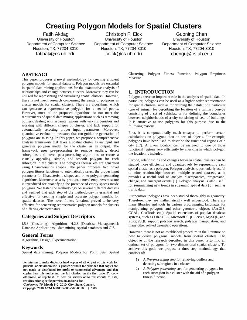
Table 1. Capabilities of each algorithm

Capability: 1 2 3 4 5 6

Convex Hull No No No Yes Yes Yes

Voronoi No No No Yes No Yes

Characteristic

shapes No No No Yes Yes Yes

Alpha shapes Yes No Yes No Yes No

s-shapes Yes Yes Yes No Yes No

Concave hull No No No Yes Yes Yes*

DContour Yes No Yes No Yes No

A-shapes Yes Yes Yes Yes No No

1: Can cope with outliers

2: Can cope with varying densities in a cluster

3: Can cope with separate regions

4: Has easy to select parameters or no parameters required

5: Does not require a separate set of points outside the cluster

6: Creates simple polygons

*unless the points are collinear

Table 1 summarizes the capabilities of each algorithm. Following

items are the most common problems with these algorithms:

Most of the algorithms cannot cope with varying densities

Many of the algorithms cannot cope with outliers

Many of the algorithms cannot cope with separate regions in

a cluster

Some algorithms require a different set of points to be

declared outside the cluster, which is not always available

Parameter selection is difficult for some algorithms

In the next section, we will introduce a comprehensive three-step

methodology that deals with all six requirements.

4. METHODOLOGY In this section, we propose a three-step methodology that

addresses the shortcomings of the existing polygon generating

algorithms, and improve the overall quality of the generated

polygons.

4.1 Pre-processing The pre-processing step deals with the following two tasks:

i. Outliers should be detected and removed before

generating clusters, so that large empty areas inside

polygons can be avoided.

ii. Well-separated regions inside clusters should be

identified. This step will decrease the amount of empty

areas that are not relevant to the cluster.

We will consider clustering algorithms for pre-processing since

clustering is a natural solution for problems involving (i) and (ii).

We reviewed the suitability of existing clustering algorithms for

the preprocessing step, based on the following requirements:

It should be easily automated, that is, its parameters should

easily be understood and selected or it should require no

parameters at all.

It should be able to cope with varying densities in the cluster.

It should be able to detect regions of arbitrary shape.

Considering the above requirements, we can eliminate many of

the clustering algorithms such as representative-based clustering

algorithms (K-MEANS, PAM), which cannot detect regions of

non-convex shapes and are sensitive to outliers. Density-based

clustering algorithms such as DBSCAN, CLIQUE, and

DENCLUE can find clusters of having non-convex shapes, but

cannot cope with varying densities and high dimensional data.

Graph-based algorithms like Jarvis Patrick (JP) [12] clustering can

cope with varying densities but it cannot cope with some datasets

if there is a bridge between clusters as demonstrated by [2].

We reviewed several clustering algorithms for the pre-processing

task and selected SNN [2] and AutoClust [13] for this task (more

details about the selection process can be found in [16]). In the

remainder, of this section we give a little more details about the

algorithms and why they were selected.

4.1.1 SNN SNN (Shared Nearest Neighbors) [2] is a density-based clustering

algorithm which assesses the similarity between two points using

the number of nearest neighbors that they share. SNN clusters

data as DBSCAN does, except that the number of shared k

neighbors is used to access the similarity instead of the Euclidean

distance. This allows the algorithm to deal with varying densities.

Similar to DBSCAN, SNN is able to find clusters of different

sizes, shapes, and can cope with noise in the dataset. Moreover,

SNN copes better with high-dimensional data.

4.1.2 AutoClust AutoClust [13] is a graph-based clustering algorithm, which

makes use of Delaunay triangulation to cluster two-dimensional

datasets. AutoClust does not require any parameters. Parameter

values are revealed from the proximity structures of the Delaunay

triangulation. Multiple bridges between clusters are detected and

removed by using a 3-step algorithm that classifies edges in each

step according to the statistical features of edges. AutoClust can

identify clusters of differing densities even in presence of outliers

and bridges between the clusters.

Authors argue that border points between clusters have a larger

standard deviation of edge lengths in Delaunay triangulation

compared to the points inside the cluster since border points have

both long edges connecting them to the points in a different

cluster and short edges connecting them to the points inside the

cluster. By using the standard deviation of edge lengths connected

to points, border points and inner cluster points are identified.

We propose using AutoClust when there is no previous

knowledge of the dataset, as it has no parameters. On the other

hand, SNN can be tuned according to the analysis task (amount of

noise, nearest neighbor size can be set) when previous knowledge

of the dataset is available as it has parameters to control the

clustering process. Fortunately, the parameters are easy to

understand and we were able to propose parameter selection

procedure that works well with most spatial clusters, allowing to

automate the pre-processing step.

4.2 Generating Polygons The pre-processing step removes outliers and partitions clusters

into well-separated subregions; therefore, the next step of the

methodology, the polygon generation step is concerned with

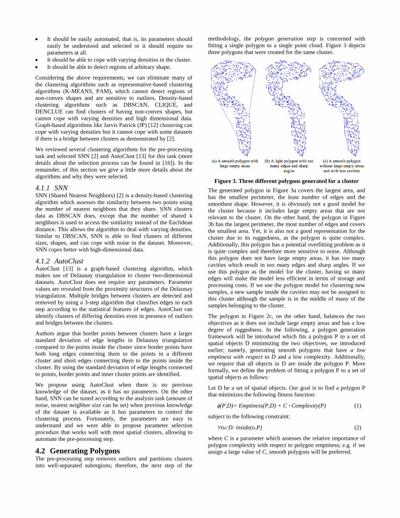
fitting a single polygon to a single point cloud. Figure 3 depicts

three polygons that were created for the same cluster.

Figure 3. Three different polygons generated for a cluster

The generated polygon in Figure 3a covers the largest area, and

has the smallest perimeter, the least number of edges and the

smoothest shape. However, it is obviously not a good model for

the cluster because it includes large empty areas that are not

relevant to the cluster. On the other hand, the polygon in Figure

3b has the largest perimeter, the most number of edges and covers

the smallest area. Yet, it is also not a good representation for the

cluster due to its ruggedness, as the polygon is quite complex.

Additionally, this polygon has a potential overfitting problem as it

is quite complex and therefore more sensitive to noise. Although

this polygon does not have large empty areas, it has too many

cavities which result in too many edges and sharp angles. If we

use this polygon as the model for the cluster, having so many

edges will make the model less efficient in terms of storage and

processing costs. If we use the polygon model for clustering new

samples, a new sample inside the cavities may not be assigned to

this cluster although the sample is in the middle of many of the

samples belonging to the cluster.

The polygon in Figure 2c, on the other hand, balances the two

objectives as it does not include large empty areas and has a low

degree of ruggedness. In the following, a polygon generation

framework will be introduced which fits a polygon P to a set of

spatial objects D minimizing the two objectives, we introduced

earlier; namely, generating smooth polygons that have a low

emptiness with respect to D and a low complexity. Additionally,

we require that all objects in D are inside the polygon P. More

formally, we define the problem of fitting a polygon P to a set of

spatial objects as follows:

Let D be a set of spatial objects. Our goal is to find a polygon P

that minimizes the following fitness function:

(P,D)= Emptiness(P,D) + C * Complexity(P) (1)

subject to the following constraint:

oD: inside(o,P) (2)

where C is a parameter which assesses the relative importance of

polygon complexity with respect to polygon emptiness; e.g. if we

assign a large value of C, smooth polygons will be preferred.

Emptiness(P,D) is a quantitative emptiness measure that assesses

the degree to which P contains empty regions with respect to D.

Complexity(P) measures the complexity of polygon P.

In the following, we first introduce our novel emptiness measure.

We then describe a polygon complexity measure that has been

defined by some other work [15] which will be reused in our

work; finally, we introduce different methods that fit polygons P

to D, solving the optimization problem described in Eq. (1).

4.2.1 Measuring the Emptiness of P with respect to D We have a surface, and we like to measure the emptiness in a

surface with respect to spatial objects embedded into it. We call a

subspace of the surface empty, if the density of the objects that are

inside the subspace is low (typically, below a user-defined

threshold). In general, we measure emptiness by computing the

sum of the volumes/areas of the empty subspaces inside the

surface over the volume/area of the surface itself.

In this particular work, we are interested in measuring the

emptiness of polygonal surfaces with respect to a set of spatial

objects D; moreover, we assume that all objects in D are located

inside the polygon P. Several approaches can be envisioned to

approach this problem. One approach is to design a non-

parametric density function based on the objects belonging to D,

and then, relying on a contouring algorithm, we can identify all

contiguous regions inside P that are empty; that is, whose density

is below a threshold ; next, we can measure emptiness by

computing the sum of the areas occupied by empty regions over

the area of the polygons P; more formally:

(P,D)=(rP: contiguous(r) empty(r) area(r))/area(P)

Figure 4: Delaunay Triangulation of a Point Cloud

However, in this paper we use a different approach, which is

based on Delaunay triangulations; in general, as can be seen in

Fig. 4, areas with very low density can be identified by large

triangles in the Delaunay triangulation; that is, triangles whose

area is above a certain size ; for example, if we use the average

triangle size in DT(D) as the threshold, the area of the large

triangle on the upper right would be identified as an empty area.

We introduce an emptiness measure which assesses the emptiness

of a polygon P with respect to a point cloud D. Let:

P be a polygon whose emptiness has to be assessed,

D a set of points in 2D that P is supposed to model,

DT(D) the set of triangles of the Delaunay triangulation of D,

be the triangle area threshold,

PCONV=(tDT(D) t) be the outer polygon of the DT(D); PCONV acts

as the surface into which the objects of D are embedded and it is

also the convex hull of D.

Our definition of emptiness of a polygon P with respect to a point

cloud D is as follows:

Emptiness(P,D):= (tDT(D)area(t)>^inside(t,P) area(t)-))/area(PCONV) (3)

When assessing emptiness of P with respect to D, we go through

the triangles inside P and add the differences between and the

area they cover, but only if the size of their area is above , and

divide this sum by the area of the convex hull of D; be aware that

pCONV is not the area P covers, but a usually larger polygon which

is the union of all triangles of Delaunay triangulation which serves

as the surface into which the object of D are embedded in. It

should be noted that when measuring emptiness triangles that are

not part of P trivially do not contribute to emptiness.

4.2.2 Measuring Polygon Complexity We assess the complexity of polygons using the polygon

complexity measure which was introduced by Brinkhoff et al.

[15]; it defines the complexity of a polygon P as follows:

Complexity(P) := 0.8 * ampl(P) * freq(P) + 0.2 * conv(P) (4)

where ampl(P) is amplitude of vibration defined as:

ampl(P) := 1 – ( boundary(convexhull(P)) / boundary(P) )

and freq(P) is the frequency of vibration of a polygon p:

freq(P) := 16 * (notchesnorm(P)-0.5)4 – 8 *

(notchesnorm(P)0.5)2 + 1

where notchesnorm(P) := notches(P) / (vertices(P)-3)

and a notch is defined as a vertex with an interior angle greater

than 180 degrees. Lastly, convexity of a polygon P is defined as:

conv(P) := 1 – ( area(P) / area(convexhull(P)) )

According to this definition, polygons with too many notches,

having significantly smaller areas and larger perimeters compared

to their convex hulls are considered complex polygons. Most

importantly, it is a suitable measure to assess the ruggedness of a

polygon model generated.

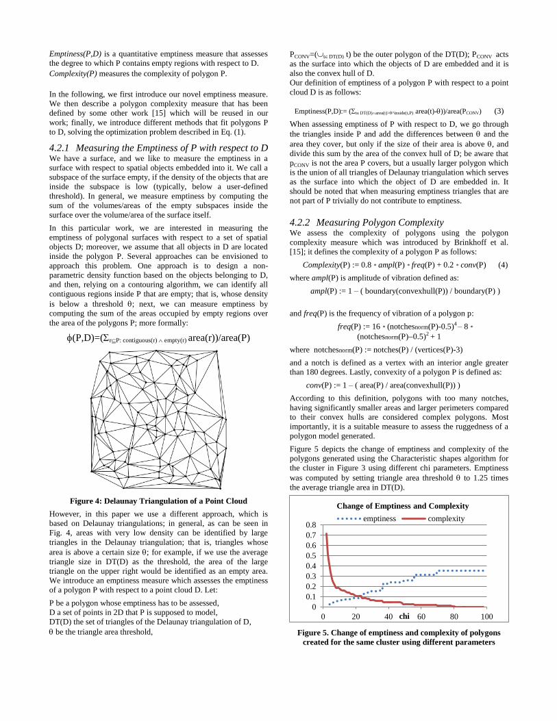
Figure 5 depicts the change of emptiness and complexity of the

polygons generated using the Characteristic shapes algorithm for

the cluster in Figure 3 using different chi parameters. Emptiness

was computed by setting triangle area threshold to 1.25 times

the average triangle area in DT(D).

Figure 5. Change of emptiness and complexity of polygons

created for the same cluster using different parameters

0

0.1

0.2

0.3

0.4

0.5

0.6

0.7

0.8

0 20 40 60 80 100chi

Change of Emptiness and Complexity

emptiness complexity

As seen in Figure 5, emptiness and complexity of the polygons are

inversely proportional. Larger chi parameters create polygons

which are emptier but less complex and vice versa. We employ

objective fitness function defined in (1) to find a balance between

the two measures.

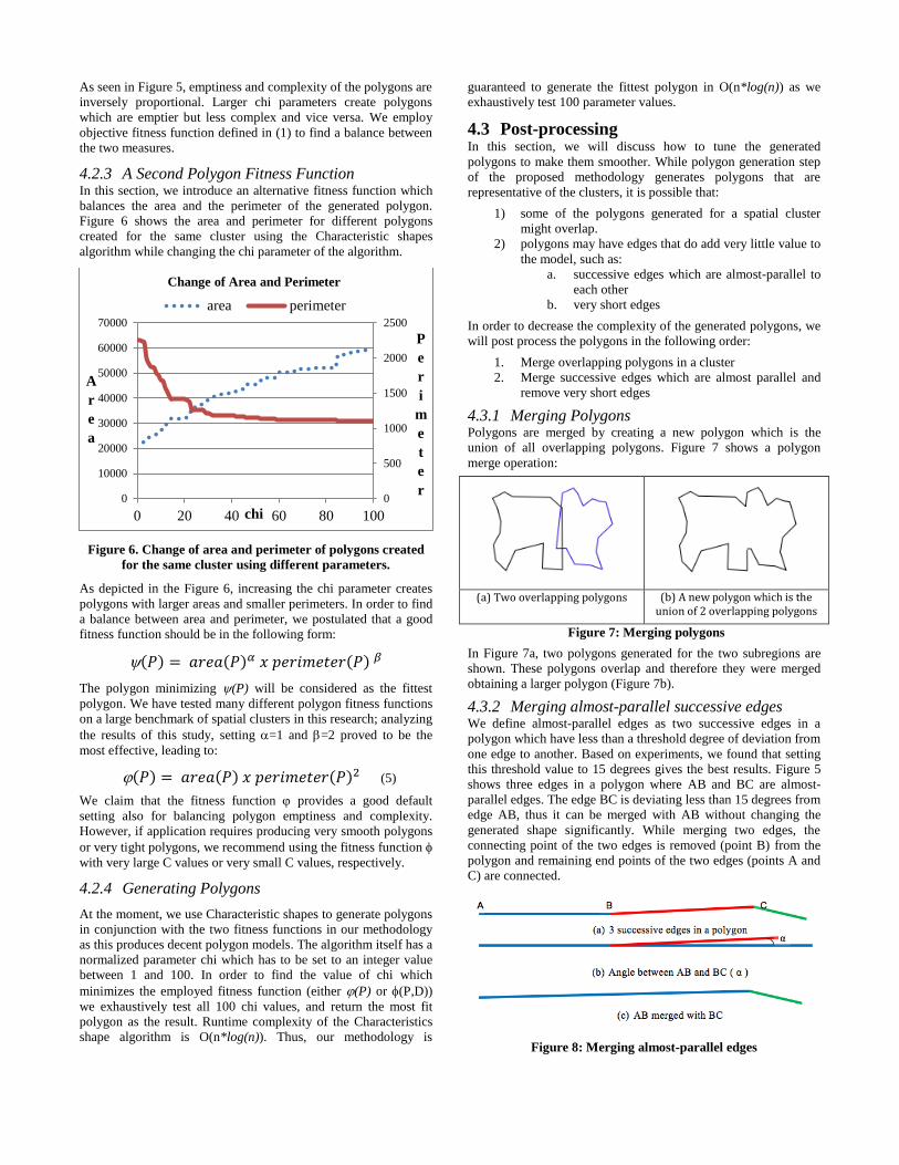
4.2.3 A Second Polygon Fitness Function In this section, we introduce an alternative fitness function which

balances the area and the perimeter of the generated polygon.

Figure 6 shows the area and perimeter for different polygons

created for the same cluster using the Characteristic shapes

algorithm while changing the chi parameter of the algorithm.

Figure 6. Change of area and perimeter of polygons created

for the same cluster using different parameters.

As depicted in the Figure 6, increasing the chi parameter creates

polygons with larger areas and smaller perimeters. In order to find

a balance between area and perimeter, we postulated that a good

fitness function should be in the following form:

( ) ( ) ( )

The polygon minimizing (P) will be considered as the fittest

polygon. We have tested many different polygon fitness functions

on a large benchmark of spatial clusters in this research; analyzing

the results of this study, setting =1 and =2 proved to be the

most effective, leading to:

( ) ( ) ( ) (5)

We claim that the fitness function provides a good default

setting also for balancing polygon emptiness and complexity.

However, if application requires producing very smooth polygons

or very tight polygons, we recommend using the fitness function

with very large C values or very small C values, respectively.

4.2.4 Generating Polygons

At the moment, we use Characteristic shapes to generate polygons

in conjunction with the two fitness functions in our methodology

as this produces decent polygon models. The algorithm itself has a

normalized parameter chi which has to be set to an integer value

between 1 and 100. In order to find the value of chi which

minimizes the employed fitness function (either (P) or (P,D))

we exhaustively test all 100 chi values, and return the most fit

polygon as the result. Runtime complexity of the Characteristics

shape algorithm is O(n*log(n)). Thus, our methodology is

guaranteed to generate the fittest polygon in O(n*log(n)) as we

exhaustively test 100 parameter values.

4.3 Post-processing In this section, we will discuss how to tune the generated

polygons to make them smoother. While polygon generation step

of the proposed methodology generates polygons that are

representative of the clusters, it is possible that:

1) some of the polygons generated for a spatial cluster

might overlap.

2) polygons may have edges that do add very little value to

the model, such as:

a. successive edges which are almost-parallel to

each other

b. very short edges

In order to decrease the complexity of the generated polygons, we

will post process the polygons in the following order:

1. Merge overlapping polygons in a cluster

2. Merge successive edges which are almost parallel and

remove very short edges

4.3.1 Merging Polygons Polygons are merged by creating a new polygon which is the

union of all overlapping polygons. Figure 7 shows a polygon

merge operation:

(a) Two overlapping polygons (b) A new polygon which is the union of 2 overlapping polygons

Figure 7: Merging polygons

In Figure 7a, two polygons generated for the two subregions are

shown. These polygons overlap and therefore they were merged

obtaining a larger polygon (Figure 7b).

4.3.2 Merging almost-parallel successive edges We define almost-parallel edges as two successive edges in a

polygon which have less than a threshold degree of deviation from

one edge to another. Based on experiments, we found that setting

this threshold value to 15 degrees gives the best results. Figure 5

shows three edges in a polygon where AB and BC are almost-

parallel edges. The edge BC is deviating less than 15 degrees from

edge AB, thus it can be merged with AB without changing the

generated shape significantly. While merging two edges, the

connecting point of the two edges is removed (point B) from the

polygon and remaining end points of the two edges (points A and

C) are connected.

Figure 8: Merging almost-parallel edges

0

500

1000

1500

2000

2500

0

10000

20000

30000

40000

50000

60000

70000

0 20 40 60 80 100

P

e

r

i

m

e

t

e

r

A

r

e

a

chi

Change of Area and Perimeter

area perimeter

Figure 9 describes the steps of the algorithm for merging two

almost-parallel edges:

foreach edge e(i) connecting points i and i+1 in the polygon

Calculate how much edge e(i+1) deviates from e(i)

If deviation is less than Θ degrees

Merge these edges by connecting points i an i+2

Increase i by 1 to skip next point

Figure 9. Pseudocode for merging two almost-parallel edges

As shown in Figure 9, once a point is removed, we increase the

counter i to skip the next edge in the polygon to avoid topological

errors.

4.3.3 Removing short edges We define short edges to have a length that is less than a threshold

edge length. By default, we set this threshold value to 20% of the

average edge length. Figure 10 shows three edges in a polygon

and how to remove edges that are very short compared to other

edges:

Figure 10. Removing short edges

Edge BC is too short; therefore it was removed from the polygon.

Removing the short edge does not change the shape significantly.

This process is similar to merging two almost-parallel edges, the

connecting point of the short edge and the previous edge (point B)

is removed and remaining end points of the two edges (points A

and C) are connected.

5. EXPERIMENTAL EVALUATION To evaluate our methodology, we created an artificial cluster

which contains some outliers that consists of 4 separated regions

which vary in density. The spatial cluster is depicted in Figure 11.

Figure 11. Artificial cluster used in the first experiment.

Figure 12 depicts a polygon that has been created using the

Characteristic shapes algorithm without using any pre-processing.

As can be seen, the generated polygon contain large empty spaces,

and the polygons obtained for other chi values were equally bad,

as Characteristic shapes creates a single polygon that contains all

the points of the spatial cluster.

Figure 12. Polygon created by the Characteristic shapes

algorithm without pre-processing

5.1 Step 1: Pre-processing When we ran SSN and AutoClust on the cluster, both algorithms

were able to detect subregions and eliminate outliers successfully.

Figure 13 depicts the subregions detected by both algorithms.

Figure 13. Pre-processing result for the cluster in Figure 11

We experimentally found that when using SNN setting the nearest

neighbors size parameter to 8 gave best results with most datasets.

SNN was able to deal with clusters of varying densities, shapes

and outliers successfully with the default parameter setting.

When we used AutoClust algorithm, we obtained the same result;

AutoClust does not have any parameters, yet it works very well on

clusters of varying densities, and shapes in presence of noise.

5.2 Step 2: Polygon Generation After detecting the 4 subregions, we generated a polygon for each

subregion in the cluster using the Characteristic shapes algorithm

in conjunction with fitness function to select the chi-parameter

values for each cluster.

The fittest polygons with respect to fitness function were

obtained at chi=43 for subregion 1, chi=24 for subregion 2,

chi=21 for subregion 3, and chi=20 for subregion 4. Figure 14

depicts the generated polygons for each subregion; as can be seen

the proposed methodology worked very well on all of the

subregions and created a representative polygon for each.

Figure 14: Polygons generated by Characteristic shapes using

fitness function .

Table 2. Properties of each polygon in Figure 14

Area Perimeter Emptiness Complexity

P1 4355 277 0.145 0.203

P2 13007 727 0.108 0.1

P3 6585 511 0.091 0.124

P4 12212 679 0.107 0.084

Next, to illustrate the benefits of the two fitness functions and

their underlying measures, we quantitatively compare the

polygons in Figure 14 with polygons that have been obtained by

running Characteristic shape with chi=10 (Figure 15) and chi=80

(Figure 16). Tables 2, 3, and 4 report the complexity, emptiness,

perimeter, and area of each polygon in Figures 14, 15, and 16,

respectively. For the emptiness calculation, we set to 1.25 times

the average area of the triangles in DT(D).

Figure 15. Generated polygons for chi=10

Table 3. Properties of each polygon in Figure 15

Area Perimeter Emptiness Complexity

P1 2505 498 0.08 0.464

P2 9528 866 0.093 0.258

P3 4547 634 0.052 0.289

P4 11478 706 0.107 0.122

Figure 16. Generated polygons for chi=80

Table 4. Properties of each polygon in Figure 16

Area Perimeter Emptiness Complexity

P1 4696 268 0.162 0.015

P2 16890 687 0.157 0.012

P3 9661 479 0.168 0.016

P4 15839 645 0.147 0.001

For chi=10, the generated polygons are very tight for subregions

1, 2 and 3, whereas for chi=80 the generated polygons are very

large for subregions 2, 3 and 4. It can also be seen as the chi-

parameter value increases polygon complexity decreases, whereas

polygon emptiness increases; for example, for the polygon created

for the second area its emptiness increases from 0.093 to 0.108 to

0.157, whereas the polygon complexity decreases from 0.464 to

0.258 to 0.012. It also can be observed that the polygon for

chi=10 is much more complex than the polygon selected by

fitness function , but this significant increase in polygon

complexity did not lead to a significant reduction in polygon

emptiness which just dropped from 0.108 to 0.093. Finally, for

each of the four subregions a different value for parameter chi was

optimal, which motivates the need to use fitness functions to

guide parameter selection.

We also created polygons using the fitness function defined in

equation 1 with the same dataset by setting C2 to 0.35 and

obtained the polygons shown in Figure 17:

2 Due to space limitations we will not report results for other C

values, and also do not analyze the results in more detail;

however, they have been reported at [18].

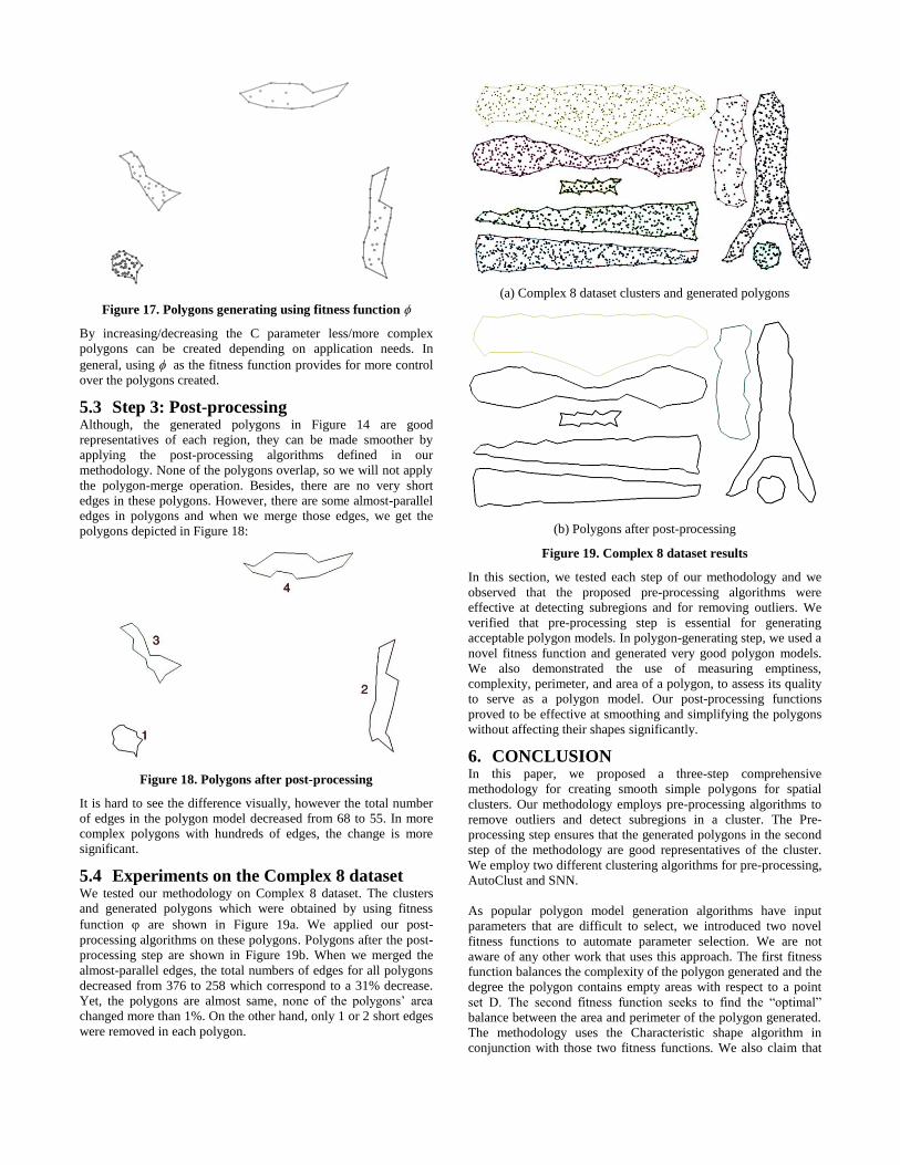
Figure 17. Polygons generating using fitness function

By increasing/decreasing the C parameter less/more complex

polygons can be created depending on application needs. In

general, using as the fitness function provides for more control

over the polygons created.

5.3 Step 3: Post-processing Although, the generated polygons in Figure 14 are good

representatives of each region, they can be made smoother by

applying the post-processing algorithms defined in our

methodology. None of the polygons overlap, so we will not apply

the polygon-merge operation. Besides, there are no very short

edges in these polygons. However, there are some almost-parallel

edges in polygons and when we merge those edges, we get the

polygons depicted in Figure 18:

Figure 18. Polygons after post-processing

It is hard to see the difference visually, however the total number

of edges in the polygon model decreased from 68 to 55. In more

complex polygons with hundreds of edges, the change is more

significant.

5.4 Experiments on the Complex 8 dataset We tested our methodology on Complex 8 dataset. The clusters

and generated polygons which were obtained by using fitness

function are shown in Figure 19a. We applied our post-

processing algorithms on these polygons. Polygons after the post-

processing step are shown in Figure 19b. When we merged the

almost-parallel edges, the total numbers of edges for all polygons

decreased from 376 to 258 which correspond to a 31% decrease.

Yet, the polygons are almost same, none of the polygons’ area

changed more than 1%. On the other hand, only 1 or 2 short edges

were removed in each polygon.

(a) Complex 8 dataset clusters and generated polygons

(b) Polygons after post-processing

Figure 19. Complex 8 dataset results

In this section, we tested each step of our methodology and we

observed that the proposed pre-processing algorithms were

effective at detecting subregions and for removing outliers. We

verified that pre-processing step is essential for generating

acceptable polygon models. In polygon-generating step, we used a

novel fitness function and generated very good polygon models.

We also demonstrated the use of measuring emptiness,

complexity, perimeter, and area of a polygon, to assess its quality

to serve as a polygon model. Our post-processing functions

proved to be effective at smoothing and simplifying the polygons

without affecting their shapes significantly.

6. CONCLUSION In this paper, we proposed a three-step comprehensive

methodology for creating smooth simple polygons for spatial

clusters. Our methodology employs pre-processing algorithms to

remove outliers and detect subregions in a cluster. The Pre-

processing step ensures that the generated polygons in the second

step of the methodology are good representatives of the cluster.

We employ two different clustering algorithms for pre-processing,

AutoClust and SNN.

As popular polygon model generation algorithms have input

parameters that are difficult to select, we introduced two novel

fitness functions to automate parameter selection. We are not

aware of any other work that uses this approach. The first fitness

function balances the complexity of the polygon generated and the

degree the polygon contains empty areas with respect to a point

set D. The second fitness function seeks to find the “optimal”

balance between the area and perimeter of the polygon generated.

The methodology uses the Characteristic shape algorithm in

conjunction with those two fitness functions. We also claim that

the proposed fitness functions can be used in conjunction with

other polygon generating algorithms, such as the concave hull

algorithms in R and in PostGIS.

We also proposed novel post-processing algorithms that merge

overlapping polygons and make the generated polygons smoother.

The complexity of the generated polygon models decrease

dramatically as a result of our post-processing methods, yet the

shapes of the polygons are not affected significantly.

Each step of the methodology was tested with different datasets

and our methodology proved to be effective at creating desired

polygon models. SNN and AutoClust successfully detected

subregions and removed outliers automatically. When used with

our polygon fitness functions, the Characteristic shapes algorithm

generated very accurate polygon models on the pre-processed

clusters. Lastly, post-processing step simplified the generated

polygon models quite significantly.

As a future work, we plan to extend our methodology to allow for

holes in polygons. We also plan to generalize our fitness

functions to be used in conjunction with other existing polygon

generating algorithms.

7. REFERENCES

[1] Wang, S., Chen, C.S., Rinsurongkawong, V., Akdag, F.

and Eick, C.F. 2010. A Polygon-based Methodology for

Mining Related Spatial Datasets. In Proc. of ACM

SIGSPATIAL International Workshop on Data Mining for

Geoinformatics (DMG) (San Jose, California).

[2] Ertoz, L., Steinbach, M., and Kumar, V. 2003. Finding

Clusters of Different Sizes, Shapes, and Densities in

Noisy, High Dimensional Data. In Proceedings of the

Second SIAM International Conference on Data Mining

(San Francisco, CA).

[3] Kargupta, H., Bhargava, R., Liu, K., Powers, M., Blair, P.,

Bushra, S., Dull, J., Sarkar, K., Klein, M., Vasa, M. and

Handy, D. 2004. VEDAS: A Mobile and Distributed Data

Stream Mining System for Real-Time Vehicle Monitoring.

In Proceedings of the Fourth SIAM International

Conference on Data Mining (Lake Buena Vista, Florida,

USA).

[4] Galton A. and Duckham, M. 2006. What is the region

occupied by a set of points? GIScience, LNCS 4197, 81–

98.

[5] Edelsbrunner, H., Kirkpatrick, D. G., and Seidel, R. 1983.

On the shape of a set of points in the plane. IEEE

Transactions on Information Theory 29,4, 551–559.

[6] Alani, H., Jones, C. B., and Tudhope, D. 2001. Voronoi-

based region approximation for geographical information

retrieval with gazetteers. International Journal of

Geographical Information Science 15, 4, 287–306.

[7] Duckham, M., Kulik, L., Worboys, M., Galton, A. 2008.

Efficient generation of simple polygons for characterizing

the shape of a set of points in the plane. Pattern

Recognition 41, 10, 3224-3236.

[8] Chaudhuri A. R., Chaudhuri B. B., and Parui S. K. 1997.

A novel approach to computation of the shape of a dot

pattern and extraction of its perceptual border. Computer

Vision and Image Understanding 68, 3, 57–275

[9] Moreira, A., Santos, M.Y. 2007. Concave hull: a k-nearest

neighbours approach for the computation of the region

occupied by a set of points. In International Conference on

Computer Graphics Theory and Applications GRAPP.

[10] Melkemi, M. and Djebali, M. 2000. Computing the shape

of a planar points set. Pattern Recognition 33, 1423–1436.

[11] Chen C.S., Rinsurongkawong V., Eick, C.F. and Twa

M.D. 2009. Change Analysis in Spatial Data by

Combining Contouring Algorithms with Supervised

Density Functions. In Proc. PAKDD (Bangkok, Thailand),

907-914.

[12] Jarvis, R. A. and Patrick, E. A. 1973, Clustering using a

similarity measure based on shared near neighbours. IEEE

Trans. on Computers, 22, 11, 1025-1034.

[13] Estivill-Castro, V. and Lee, I. 2002. Argument free

clustering for large spatial point-data sets via boundary

extraction from Delaunay diagram. Computers,

Environment and Urban Systems, 26, 4, 315-334.

[14] Jarvis, R. A. 1973. On the identification of the convex hull

of a finite set of points in the plane. Information

Processing Letters 2, 18–21.

[15] Brinkhoff, T., Kriegel, H.-P., Schneider, R., Braun, A.

1995, Measuring the Complexity of Polygonal Objects.

Proc. of the Third ACM International Workshop on

Advances in Geographical Information Systems, 109-117

[16] Akdag, F. 2010. Algorithms for Creating Polygon Models

for Spatial Clusters, Master’s Thesis, University of

Houston (Houston, Texas).

[17] Z. Cao, S. Wang, G. Forestier, A. Puissant, and C. F. Eick.

August 2013. Analyzing the Composition of Cities Using

Spatial Clustering, in Proc. 2nd ACM SIGKDD

International Workshop on Urban Computing, (Chicago,

Illinois).

[18] Akdag, F. 2013. Supplement for paper "Creating Polygon

Models for Spatial Clusters". Retrieved June 30, 2013

from http://www2.cs.uh.edu/~ceick/kdd/AEC13-

supplements.docx