i 

 

 

Creating Performance Curves for Variable Refrigerant Flow Heat Pumps in EnergyPlus

 

FSEC-CR-1910-12

March 8, 2012 (revised November 21, 2012)

Contract Report

Technical Subtopic 2.1: Modeling Variable Refrigerant Flow Heat Pump and Heat Recovery Equipment in EnergyPlus

DOE/NETL Award DE-EE0003848

 

Author

Richard Raustad

Copyright ©2009 Florida Solar Energy Center/University of Central Florida 

All Rights Reserved. 

2 

 

 

Disclaimer 

The Florida Solar Energy Center/University of Central Florida nor any agency thereof, nor any of their 

employees, makes any warranty, express or implied, or assumes any legal liability or responsibility for 

the accuracy, completeness, or usefulness of any information, apparatus, product, or process disclosed, 

or represents that its use would not infringe privately owned rights. Reference herein to any specific 

commercial product, process, or service by trade name, trademark, manufacturer, or otherwise does 

not necessarily constitute or imply its endorsement, recommendation, or favoring by the Florida Solar 

Energy Center/University of Central Florida or any agency thereof. The views and opinions of authors 

expressed herein do not necessarily state or reflect those of the Florida Solar Energy Center/University 

of Central Florida or any agency thereof.  

3 

 

 

Acknowledgment 

This material is based upon work supported by the Department of Energy under Award Numbers DE-EE0003848.

Disclaimer: "This report was prepared as an account of work sponsored by an agency of the United States

Government. Neither the United States Government nor any agency thereof, nor any of their employees, makes any

warranty, express or implied, or assumes any legal liability or responsibility for the accuracy, completeness, or

usefulness of any information, apparatus, product, or process disclosed, or represents that its use would not infringe

privately owned rights. Reference herein to any specific commercial product, process, or service by trade name,

trademark, manufacturer, or otherwise does not necessarily constitute or imply its endorsement, recommendation, or

favoring by the United States Government or any agency thereof. The views and opinions of authors expressed

herein do not necessarily state or reflect those of the United States Government or any agency thereof."

4 

 

 

TableofContents

ABSTRACT ...................................................................................................................................................... 5 

Introduction .................................................................................................................................................. 5 

Cooling Performance Curves ......................................................................................................................... 6 

Cooling Capacity Ratio Modifier Performance Curve ................................................................................... 9 

Application of Dual Performance Curves .................................................................................................... 10 

Cooling Capacity Ratio Modifier Function of Low Temperatures ............................................................... 10 

Cooling Capacity Ratio Boundary Curve ..................................................................................................... 13 

Cooling Capacity Ratio Modifier Function of High Temperatures .............................................................. 14 

Cooling Energy Input Ratio Modifier ........................................................................................................... 21 

Cooling Energy Input Ratio Modifier Function of Part‐Load Ratio ............................................................. 25 

Cooling Energy Input Ratio Modifier Function of Low Part‐Load Ratio ...................................................... 28 

Cooling Energy Input Ratio Modifier Function of High Part‐Load Ratio ..................................................... 29 

Cooling Combination Ratio Correction Factor ............................................................................................ 29 

Cooling Part‐Load Fraction Correlation Curve ............................................................................................ 33 

Piping Correction Factors ............................................................................................................................ 34 

Piping Correction Factor for Length in Cooling Mode ................................................................................ 34 

Piping Correction Factor for Height in Cooling Mode ................................................................................. 38 

Heating Operation ...................................................................................................................................... 38 

 

 

5 

 

ABSTRACT

This document describes methods to generate performance curve coefficients for variable refrigerant flow heat pumps in DOE’s EnergyPlus building energy simulation program. Manufactures performance data for capacity and power are used to create full-load and part-load performance curves for cooling and heating operating modes. When performance variations for full-load capacity or power cannot be modeled using a single performance curve, the data set is divided into lower and upper temperature regions and dual performance curves are used. Table objects may also be created to substitute when performance curves do not provide the required accuracy. These performance curves or tables are then used as input data for the variable refrigerant flow heat pump model. The techniques described in this paper can be used to create performance curves for any EnergyPlus equipment model

Introduction

The variable refrigerant flow (VRF) heat pump air conditioner (AC) is a heating, ventilating, and air-conditioning (HVAC) model in the United States Department of Energy’s (DOE) EnergyPlus building energy simulation program. The performance of a VRF AC system is based on multiple performance characteristics. Full-load performance data defines the variations of capacity and power when outdoor or indoor conditions change. Part-load performance identifies how the capacity and power change when the heat pump condenser’s variable compressor changes speed. The performance of a VRF AC system may also change when the total indoor terminal unit capacity is greater than the total outdoor unit capacity. The ratio of indoor terminal unit to outdoor condenser unit capacity is referred to as the combination ratio (CR). These performance aspects will be described in detail throughout this paper.

The key model inputs required to accurately simulate a VRF AC system are the rated capacity and coefficient of performance, the operating limits of the condenser, and the performance curves used to model variations in capacity and power. Piping losses are also modeled based on the length and height of the refrigerant lines. The heat pump VRF AC system can operate in either cooling or heating mode (no simultaneous cooling and heating) and selects the operating mode based on a select control strategy. The inputs for the VRF AC model are the same for both cooling and heating.

The cooling model inputs for a VRF AC system are:

Rated Total Cooling Capacity

Rated Cooling COP

Minimum Outdoor Temperature in Cooling Mode

Maximum Outdoor Temperature in Cooling Mode

Cooling Capacity Ratio Modifier Function of Low Temperature Curve Name

Cooling Capacity Ratio Boundary Curve Name

Cooling Capacity Ratio Modifier Function of High Temperature Curve Name

Cooling Energy Input Ratio Modifier Function of Low Temperature Curve Name

Cooling Energy Input Ratio Boundary Curve Name

Cooling Energy Input Ratio Modifier Function of High Temperature Curve Name

Cooling Energy Input Ratio Modifier Function of Low Part-Load Ratio Curve Name

6 

 

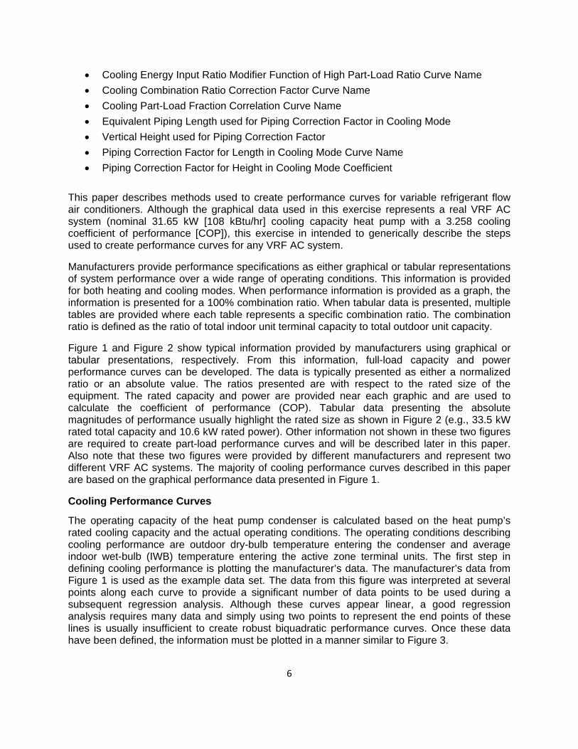
Cooling Energy Input Ratio Modifier Function of High Part-Load Ratio Curve Name

Cooling Combination Ratio Correction Factor Curve Name

Cooling Part-Load Fraction Correlation Curve Name

Equivalent Piping Length used for Piping Correction Factor in Cooling Mode

Vertical Height used for Piping Correction Factor

Piping Correction Factor for Length in Cooling Mode Curve Name

Piping Correction Factor for Height in Cooling Mode Coefficient

This paper describes methods used to create performance curves for variable refrigerant flow air conditioners. Although the graphical data used in this exercise represents a real VRF AC system (nominal 31.65 kW [108 kBtu/hr] cooling capacity heat pump with a 3.258 cooling coefficient of performance [COP]), this exercise in intended to generically describe the steps used to create performance curves for any VRF AC system.

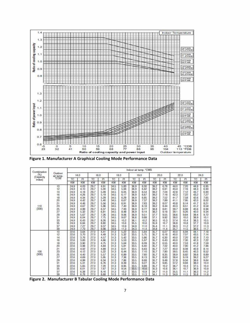
Manufacturers provide performance specifications as either graphical or tabular representations of system performance over a wide range of operating conditions. This information is provided for both heating and cooling modes. When performance information is provided as a graph, the information is presented for a 100% combination ratio. When tabular data is presented, multiple tables are provided where each table represents a specific combination ratio. The combination ratio is defined as the ratio of total indoor unit terminal capacity to total outdoor unit capacity.

Figure 1 and Figure 2 show typical information provided by manufacturers using graphical or tabular presentations, respectively. From this information, full-load capacity and power performance curves can be developed. The data is typically presented as either a normalized ratio or an absolute value. The ratios presented are with respect to the rated size of the equipment. The rated capacity and power are provided near each graphic and are used to calculate the coefficient of performance (COP). Tabular data presenting the absolute magnitudes of performance usually highlight the rated size as shown in Figure 2 (e.g., 33.5 kW rated total capacity and 10.6 kW rated power). Other information not shown in these two figures are required to create part-load performance curves and will be described later in this paper. Also note that these two figures were provided by different manufacturers and represent two different VRF AC systems. The majority of cooling performance curves described in this paper are based on the graphical performance data presented in Figure 1.

Cooling Performance Curves

The operating capacity of the heat pump condenser is calculated based on the heat pump’s rated cooling capacity and the actual operating conditions. The operating conditions describing cooling performance are outdoor dry-bulb temperature entering the condenser and average indoor wet-bulb (IWB) temperature entering the active zone terminal units. The first step in defining cooling performance is plotting the manufacturer’s data. The manufacturer’s data from Figure 1 is used as the example data set. The data from this figure was interpreted at several points along each curve to provide a significant number of data points to be used during a subsequent regression analysis. Although these curves appear linear, a good regression analysis requires many data and simply using two points to represent the end points of these lines is usually insufficient to create robust biquadratic performance curves. Once these data have been defined, the information must be plotted in a manner similar to Figure 3.

7 

 

 Figure 1. Manufacturer A Graphical Cooling Mode Performance Data 

 Figure 2.  Manufacturer B Tabular Cooling Mode Performance Data 

8 

 

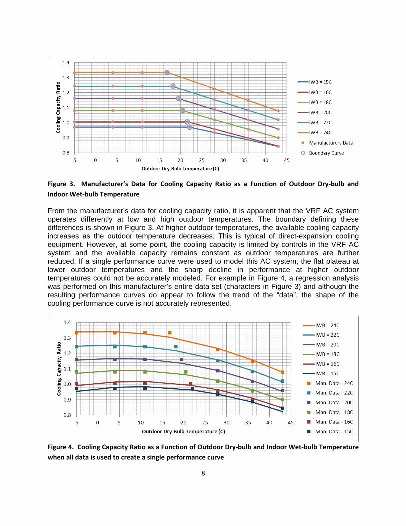
 Figure  3.   Manufacturer’s  Data  for  Cooling  Capacity  Ratio  as  a  Function  of Outdoor  Dry‐bulb  and 

Indoor Wet‐bulb Temperature

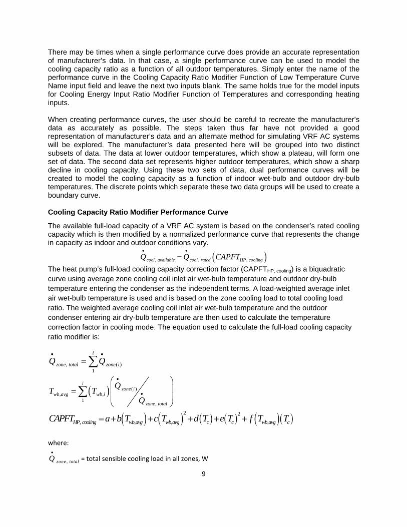
From the manufacturer’s data for cooling capacity ratio, it is apparent that the VRF AC system operates differently at low and high outdoor temperatures. The boundary defining these differences is shown in Figure 3. At higher outdoor temperatures, the available cooling capacity increases as the outdoor temperature decreases. This is typical of direct-expansion cooling equipment. However, at some point, the cooling capacity is limited by controls in the VRF AC system and the available capacity remains constant as outdoor temperatures are further reduced. If a single performance curve were used to model this AC system, the flat plateau at lower outdoor temperatures and the sharp decline in performance at higher outdoor temperatures could not be accurately modeled. For example in Figure 4, a regression analysis was performed on this manufacturer’s entire data set (characters in Figure 3) and although the resulting performance curves do appear to follow the trend of the “data”, the shape of the cooling performance curve is not accurately represented.

 Figure 4.  Cooling Capacity Ratio as a Function of Outdoor Dry‐bulb and Indoor Wet‐bulb Temperature 

when all data is used to create a single performance curve 

9 

 

There may be times when a single performance curve does provide an accurate representation of manufacturer’s data. In that case, a single performance curve can be used to model the cooling capacity ratio as a function of all outdoor temperatures. Simply enter the name of the performance curve in the Cooling Capacity Ratio Modifier Function of Low Temperature Curve Name input field and leave the next two inputs blank. The same holds true for the model inputs for Cooling Energy Input Ratio Modifier Function of Temperatures and corresponding heating inputs. When creating performance curves, the user should be careful to recreate the manufacturer’s data as accurately as possible. The steps taken thus far have not provided a good representation of manufacturer’s data and an alternate method for simulating VRF AC systems will be explored. The manufacturer’s data presented here will be grouped into two distinct subsets of data. The data at lower outdoor temperatures, which show a plateau, will form one set of data. The second data set represents higher outdoor temperatures, which show a sharp decline in cooling capacity. Using these two sets of data, dual performance curves will be created to model the cooling capacity as a function of indoor wet-bulb and outdoor dry-bulb temperatures. The discrete points which separate these two data groups will be used to create a boundary curve. Cooling Capacity Ratio Modifier Performance Curve

The available full-load capacity of a VRF AC system is based on the condenser’s rated cooling capacity which is then modified by a normalized performance curve that represents the change in capacity as indoor and outdoor conditions vary.

, , ,cool available cool rated HP coolingQ Q CAPFT

The heat pump’s full-load cooling capacity correction factor (CAPFTHP, cooling) is a biquadratic curve using average zone cooling coil inlet air wet-bulb temperature and outdoor dry-bulb temperature entering the condenser as the independent terms. A load-weighted average inlet air wet-bulb temperature is used and is based on the zone cooling load to total cooling load ratio. The weighted average cooling coil inlet air wet-bulb temperature and the outdoor condenser entering air dry-bulb temperature are then used to calculate the temperature correction factor in cooling mode. The equation used to calculate the full-load cooling capacity ratio modifier is: 

, ( )1

i

zone total zone iQ Q

( ), ,

1,

izone i

wb avg wb i

zone total

QT T

Q

2 2

, , , ,HP cooling wb avg wb avg c c wb avg cCAPFT a b T c T d T e T f T T

 

where: 

,zone totalQ

= total sensible cooling load in all zones, W 

10 

 

( )zone iQ

= zone sensible cooling load in zone I, W 

,w b a vgT = load‐weighted average wet‐bulb temperature of the air entering all operating cooling coils, °C 

,w b iT = wet‐bulb temperature of air entering the cooling coil in zone I, °C 

,HP coolingCAPFT = heat pump capacity correction factor for temperatures in cooling mode 

cT = heat pump condenser entering air dry‐bulb temperature, °C 

a f = performance curve coefficients 

Application of Dual Performance Curves

Referring again to the manufacturer’s data in Figure 3, the performance can be separated into two distinct regions. One data set is used to represent the cooling capacity ratio at low outdoor temperatures and the other data set is used to represent the cooling capacity ratio at high outdoor temperatures. A boundary curve is also required to discern between these two cooling capacity ratio curves. Manufacturer’s data to the left of the boundary curve will be used to create the Cooling Capacity Ratio Modifier Function of Low Temperature curve coefficients, and data to the right of the boundary curve will be used to create the Cooling Capacity Ratio Modifier Function of High Temperature curve coefficients. The data that define the change in performance (identified by blue circles) will be used to create the Cooling Capacity Ratio Boundary curve coefficients. Note that the boundary curve data will be included in both low and high outdoor temperature data sets. Cooling Capacity Ratio Modifier Function of Low Temperatures

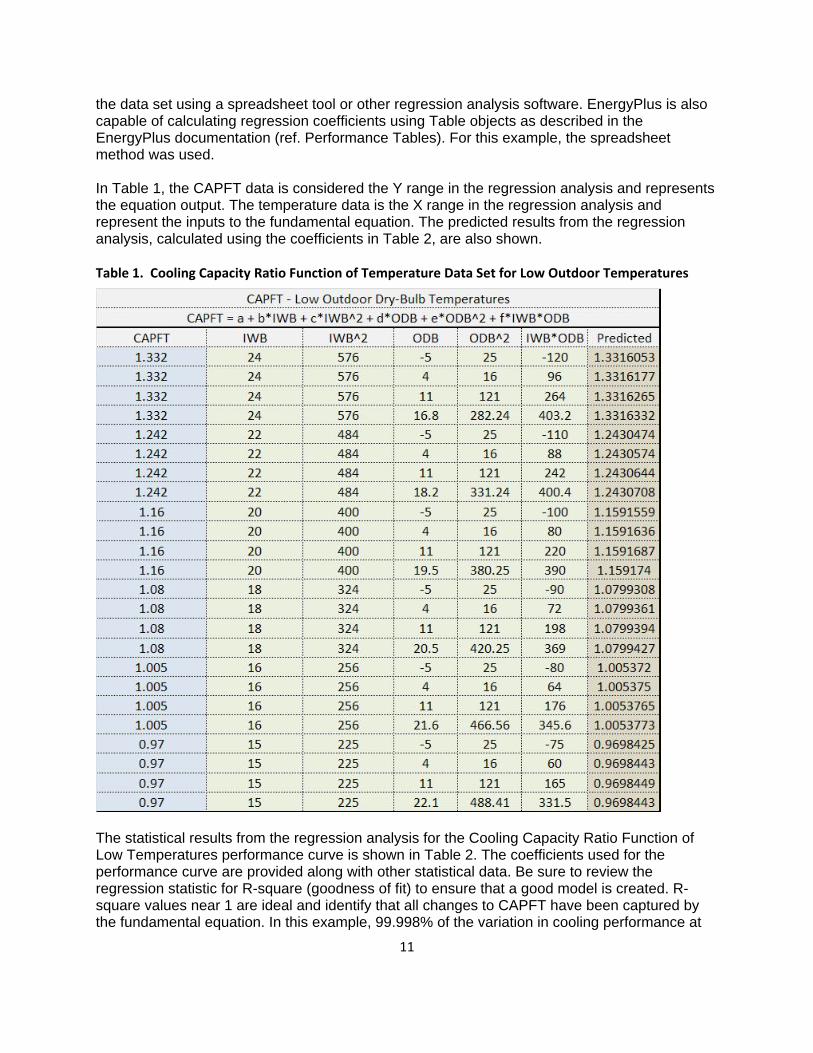
Select the data from Figure 3 that represent the cooling capacity ratio at low outdoor temperatures (i.e., data to the left of and including the boundary curve) and organize the indoor and outdoor temperatures according to the fundamental form of the CAPFT equation. Keep in mind that even though the performance of this AC unit was linear at both low and high outdoor temperatures and only two data points are required to model a straight line, that many data should be used to accurately define the performance in both temperature regions. Table 1 shows a typical spreadsheet layout of this data. The data in this table were read directly from the graph in Figure 1. The CAPFT column represents the normalized ratio of actual cooling capacity to the rated total cooling capacity at the specific operating conditions. When tabular data is used, the data is typically presented as capacity, in Watts or Btu/hr, and must be converted to a cooling capacity ratio term (i.e., the data must be normalized). In this case, select a reference point from the data set (or use the manufacturer’s rated cooling capacity). A typical rating point is 35°C outdoor dry-bulb temperature and 19.4°C indoor wet-bulb temperature. Actually any reference point may be used, but once the reference point is selected do not change it for the remainder of the regression analysis. Divide all capacity data by the Rated Total Cooling Capacity to yield cooling capacity ratio. If tabular data is used, there will most likely be a 1 in the CAPFT column where the indoor wet-bulb (IWB) and outdoor dry-bulb (ODB) temperatures match the rating point. When the data used for regression analysis is non-linear, there will typically be many more data points than are shown in this example. Make sure to use as many points as necessary to accurately represent the VRF AC system performance. Then perform a regression analysis on

11 

 

the data set using a spreadsheet tool or other regression analysis software. EnergyPlus is also capable of calculating regression coefficients using Table objects as described in the EnergyPlus documentation (ref. Performance Tables). For this example, the spreadsheet method was used. In Table 1, the CAPFT data is considered the Y range in the regression analysis and represents the equation output. The temperature data is the X range in the regression analysis and represent the inputs to the fundamental equation. The predicted results from the regression analysis, calculated using the coefficients in Table 2, are also shown. Table 1.  Cooling Capacity Ratio Function of Temperature Data Set for Low Outdoor Temperatures 

The statistical results from the regression analysis for the Cooling Capacity Ratio Function of Low Temperatures performance curve is shown in Table 2. The coefficients used for the performance curve are provided along with other statistical data. Be sure to review the regression statistic for R-square (goodness of fit) to ensure that a good model is created. R-square values near 1 are ideal and identify that all changes to CAPFT have been captured by the fundamental equation. In this example, 99.998% of the variation in cooling performance at

12 

 

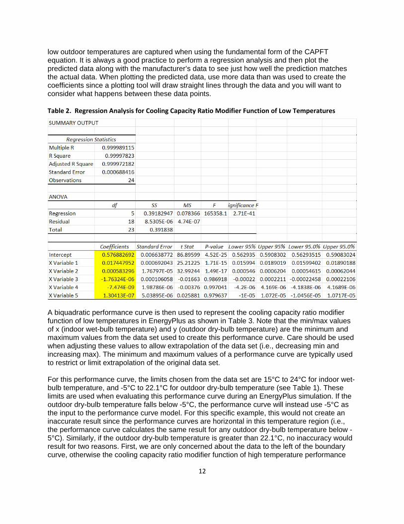
low outdoor temperatures are captured when using the fundamental form of the CAPFT equation. It is always a good practice to perform a regression analysis and then plot the predicted data along with the manufacturer’s data to see just how well the prediction matches the actual data. When plotting the predicted data, use more data than was used to create the coefficients since a plotting tool will draw straight lines through the data and you will want to consider what happens between these data points. Table 2.  Regression Analysis for Cooling Capacity Ratio Modifier Function of Low Temperatures 

A biquadratic performance curve is then used to represent the cooling capacity ratio modifier function of low temperatures in EnergyPlus as shown in Table 3. Note that the min/max values of x (indoor wet-bulb temperature) and y (outdoor dry-bulb temperature) are the minimum and maximum values from the data set used to create this performance curve. Care should be used when adjusting these values to allow extrapolation of the data set (i.e., decreasing min and increasing max). The minimum and maximum values of a performance curve are typically used to restrict or limit extrapolation of the original data set. For this performance curve, the limits chosen from the data set are 15°C to 24°C for indoor wet-bulb temperature, and -5°C to 22.1°C for outdoor dry-bulb temperature (see Table 1). These limits are used when evaluating this performance curve during an EnergyPlus simulation. If the outdoor dry-bulb temperature falls below -5°C, the performance curve will instead use -5°C as the input to the performance curve model. For this specific example, this would not create an inaccurate result since the performance curves are horizontal in this temperature region (i.e., the performance curve calculates the same result for any outdoor dry-bulb temperature below -5°C). Similarly, if the outdoor dry-bulb temperature is greater than 22.1°C, no inaccuracy would result for two reasons. First, we are only concerned about the data to the left of the boundary curve, otherwise the cooling capacity ratio modifier function of high temperature performance

13 

 

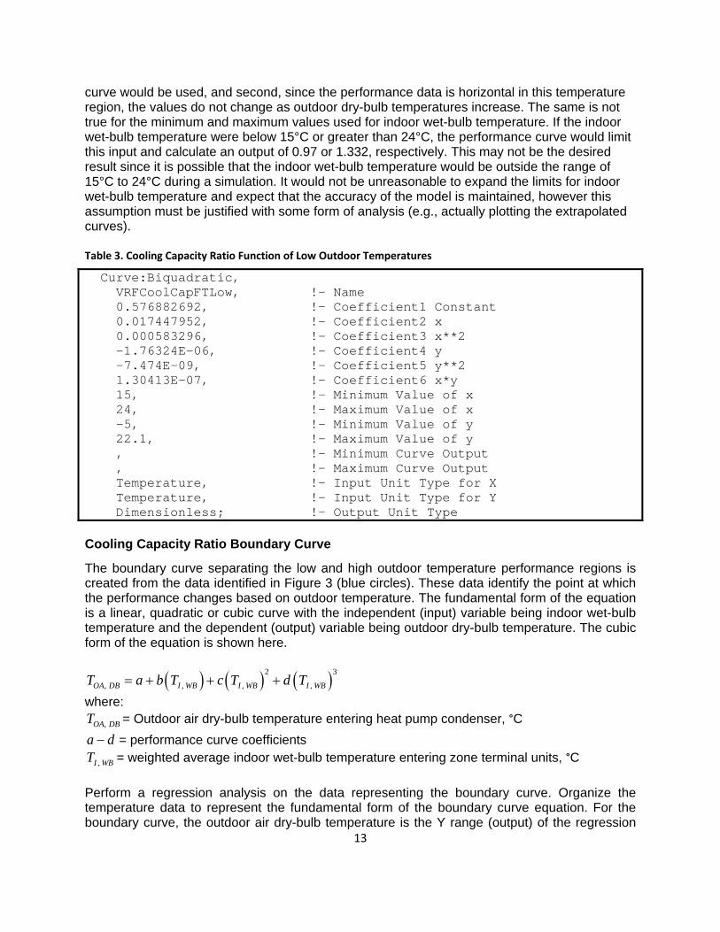
curve would be used, and second, since the performance data is horizontal in this temperature region, the values do not change as outdoor dry-bulb temperatures increase. The same is not true for the minimum and maximum values used for indoor wet-bulb temperature. If the indoor wet-bulb temperature were below 15°C or greater than 24°C, the performance curve would limit this input and calculate an output of 0.97 or 1.332, respectively. This may not be the desired result since it is possible that the indoor wet-bulb temperature would be outside the range of 15°C to 24°C during a simulation. It would not be unreasonable to expand the limits for indoor wet-bulb temperature and expect that the accuracy of the model is maintained, however this assumption must be justified with some form of analysis (e.g., actually plotting the extrapolated curves). Table 3. Cooling Capacity Ratio Function of Low Outdoor Temperatures 

Curve:Biquadratic, VRFCoolCapFTLow, !- Name 0.576882692, !- Coefficient1 Constant 0.017447952, !- Coefficient2 x 0.000583296, !- Coefficient3 x**2 -1.76324E-06, !- Coefficient4 y -7.474E-09, !- Coefficient5 y**2 1.30413E-07, !- Coefficient6 x*y 15, !- Minimum Value of x 24, !- Maximum Value of x -5, !- Minimum Value of y 22.1, !- Maximum Value of y , !- Minimum Curve Output , !- Maximum Curve Output Temperature, !- Input Unit Type for X Temperature, !- Input Unit Type for Y Dimensionless; !- Output Unit Type Cooling Capacity Ratio Boundary Curve

The boundary curve separating the low and high outdoor temperature performance regions is created from the data identified in Figure 3 (blue circles). These data identify the point at which the performance changes based on outdoor temperature. The fundamental form of the equation is a linear, quadratic or cubic curve with the independent (input) variable being indoor wet-bulb temperature and the dependent (output) variable being outdoor dry-bulb temperature. The cubic form of the equation is shown here.

2 3

, , , ,OA DB I WB I WB I WBT a b T c T d T

where:

,OA DBT = Outdoor air dry-bulb temperature entering heat pump condenser, °C

a d = performance curve coefficients

,I WBT = weighted average indoor wet-bulb temperature entering zone terminal units, °C

Perform a regression analysis on the data representing the boundary curve. Organize the temperature data to represent the fundamental form of the boundary curve equation. For the boundary curve, the outdoor air dry-bulb temperature is the Y range (output) of the regression

14 

 

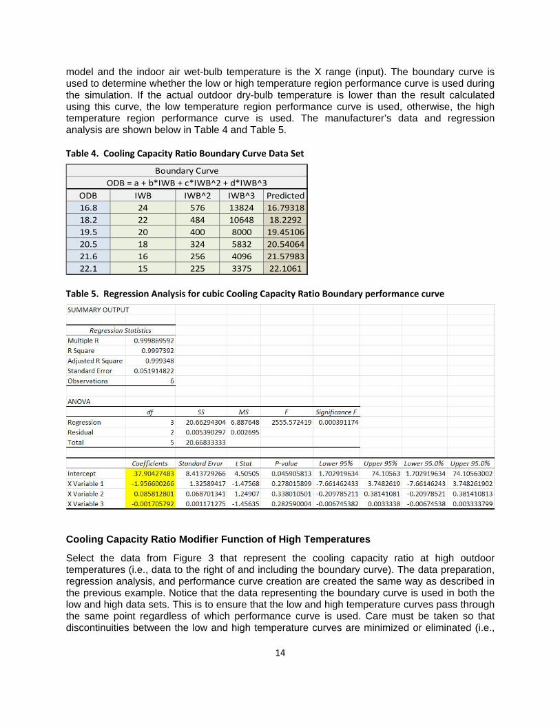
model and the indoor air wet-bulb temperature is the X range (input). The boundary curve is used to determine whether the low or high temperature region performance curve is used during the simulation. If the actual outdoor dry-bulb temperature is lower than the result calculated using this curve, the low temperature region performance curve is used, otherwise, the high temperature region performance curve is used. The manufacturer’s data and regression analysis are shown below in Table 4 and Table 5. Table 4.  Cooling Capacity Ratio Boundary Curve Data Set 

ODB IWB IWB^2 IWB^3 Predicted

16.8 24 576 13824 16.79318

18.2 22 484 10648 18.2292

19.5 20 400 8000 19.45106

20.5 18 324 5832 20.54064

21.6 16 256 4096 21.57983

22.1 15 225 3375 22.1061

Boundary Curve

ODB = a + b*IWB + c*IWB^2 + d*IWB^3

   Table 5.  Regression Analysis for cubic Cooling Capacity Ratio Boundary performance curve 

   Cooling Capacity Ratio Modifier Function of High Temperatures

Select the data from Figure 3 that represent the cooling capacity ratio at high outdoor temperatures (i.e., data to the right of and including the boundary curve). The data preparation, regression analysis, and performance curve creation are created the same way as described in the previous example. Notice that the data representing the boundary curve is used in both the low and high data sets. This is to ensure that the low and high temperature curves pass through the same point regardless of which performance curve is used. Care must be taken so that discontinuities between the low and high temperature curves are minimized or eliminated (i.e.,

15 

 

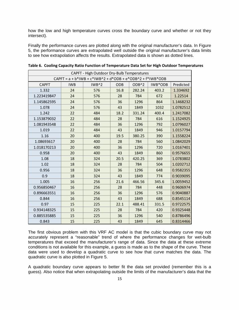
how the low and high temperature curves cross the boundary curve and whether or not they intersect). Finally the performance curves are plotted along with the original manufacturer’s data. In Figure 5, the performance curves are extrapolated well outside the original manufacturer’s data limits to see how extrapolation affects the results. Extrapolated data is shown as dotted lines. Table 6.  Cooling Capacity Ratio Function of Temperature Data Set for High Outdoor Temperatures 

CAPFT IWB IWB^2 ODB ODB^2 IWB*ODB Predicted

1.332 24 576 16.8 282.24 403.2 1.334692

1.223419847 24 576 28 784 672 1.22514

1.145862595 24 576 36 1296 864 1.1468232

1.078 24 576 43 1849 1032 1.0782512

1.242 22 484 18.2 331.24 400.4 1.2417082

1.153879032 22 484 28 784 616 1.1524925

1.081943548 22 484 36 1296 792 1.0796027

1.019 22 484 43 1849 946 1.0157794

1.16 20 400 19.5 380.25 390 1.1558224

1.08693617 20 400 28 784 560 1.0842029

1.018170213 20 400 36 1296 720 1.0167401

0.958 20 400 43 1849 860 0.9576655

1.08 18 324 20.5 420.25 369 1.0783802

1.02 18 324 28 784 504 1.0202712

0.956 18 324 36 1296 648 0.9582355

0.9 18 324 43 1849 774 0.9039095

1.005 16 256 21.6 466.56 345.6 1.0059452

0.956850467 16 256 28 784 448 0.9606974

0.896663551 16 256 36 1296 576 0.9040887

0.844 16 256 43 1849 688 0.8545114

0.97 15 225 22.1 488.41 331.5 0.9722575

0.934148325 15 225 28 784 420 0.9325448

0.885535885 15 225 36 1296 540 0.8786496

0.843 15 225 43 1849 645 0.8314466

CAPFT = a + b*IWB + c*IWB^2 + d*ODB + e*ODB^2 + f*IWB*ODB

CAPFT ‐ High Outdoor Dry‐Bulb Temperatures

   The first obvious problem with this VRF AC model is that the cubic boundary curve may not accurately represent a “reasonable” trend of where the performance changes for wet-bulb temperatures that exceed the manufacturer’s range of data. Since the data at these extreme conditions is not available for this example, a guess is made as to the shape of the curve. These data were used to develop a quadratic curve to see how that curve matches the data. The quadratic curve is also plotted in Figure 5. A quadratic boundary curve appears to better fit the data set provided (remember this is a guess). Also notice that when extrapolating outside the limits of the manufacturer’s data that the

16 

 

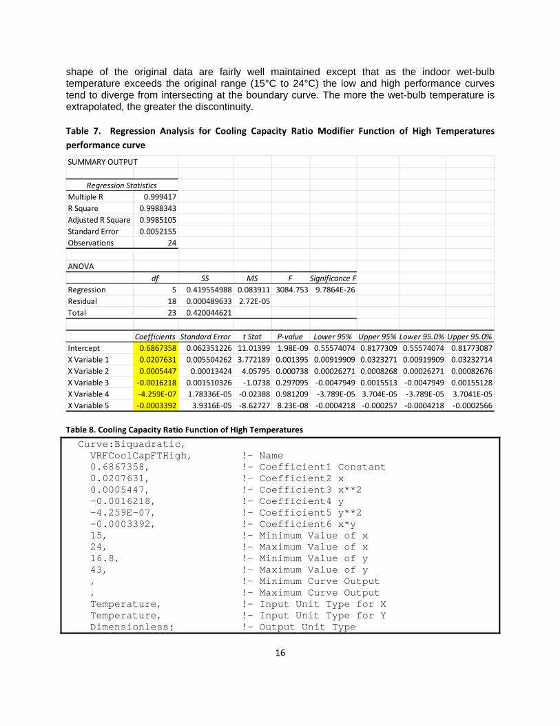
shape of the original data are fairly well maintained except that as the indoor wet-bulb temperature exceeds the original range (15°C to 24°C) the low and high performance curves tend to diverge from intersecting at the boundary curve. The more the wet-bulb temperature is extrapolated, the greater the discontinuity.  Table  7.    Regression  Analysis  for  Cooling  Capacity  Ratio Modifier  Function  of  High  Temperatures 

performance curve 

SUMMARY OUTPUT

Regression Statistics

Multiple R 0.999417

R Square 0.9988343

Adjusted R Square 0.9985105

Standard Error 0.0052155

Observations 24

ANOVA

df SS MS F Significance F

Regression 5 0.419554988 0.083911 3084.753 9.7864E‐26

Residual 18 0.000489633 2.72E‐05

Total 23 0.420044621

Coefficients Standard Error t Stat P‐value Lower 95% Upper 95% Lower 95.0% Upper 95.0%

Intercept 0.6867358 0.062351226 11.01399 1.98E‐09 0.55574074 0.8177309 0.55574074 0.81773087

X Variable 1 0.0207631 0.005504262 3.772189 0.001395 0.00919909 0.0323271 0.00919909 0.03232714

X Variable 2 0.0005447 0.00013424 4.05795 0.000738 0.00026271 0.0008268 0.00026271 0.00082676

X Variable 3 ‐0.0016218 0.001510326 ‐1.0738 0.297095 ‐0.0047949 0.0015513 ‐0.0047949 0.00155128

X Variable 4 ‐4.259E‐07 1.78336E‐05 ‐0.02388 0.981209 ‐3.789E‐05 3.704E‐05 ‐3.789E‐05 3.7041E‐05

X Variable 5 ‐0.0003392 3.9316E‐05 ‐8.62727 8.23E‐08 ‐0.0004218 ‐0.000257 ‐0.0004218 ‐0.0002566    Table 8. Cooling Capacity Ratio Function of High Temperatures 

Curve:Biquadratic, VRFCoolCapFTHigh, !- Name 0.6867358, !- Coefficient1 Constant 0.0207631, !- Coefficient2 x 0.0005447, !- Coefficient3 x**2 -0.0016218, !- Coefficient4 y -4.259E-07, !- Coefficient5 y**2 -0.0003392, !- Coefficient6 x*y 15, !- Minimum Value of x 24, !- Maximum Value of x 16.8, !- Minimum Value of y 43, !- Maximum Value of y , !- Minimum Curve Output , !- Maximum Curve Output Temperature, !- Input Unit Type for X Temperature, !- Input Unit Type for Y Dimensionless; !- Output Unit Type

17 

 

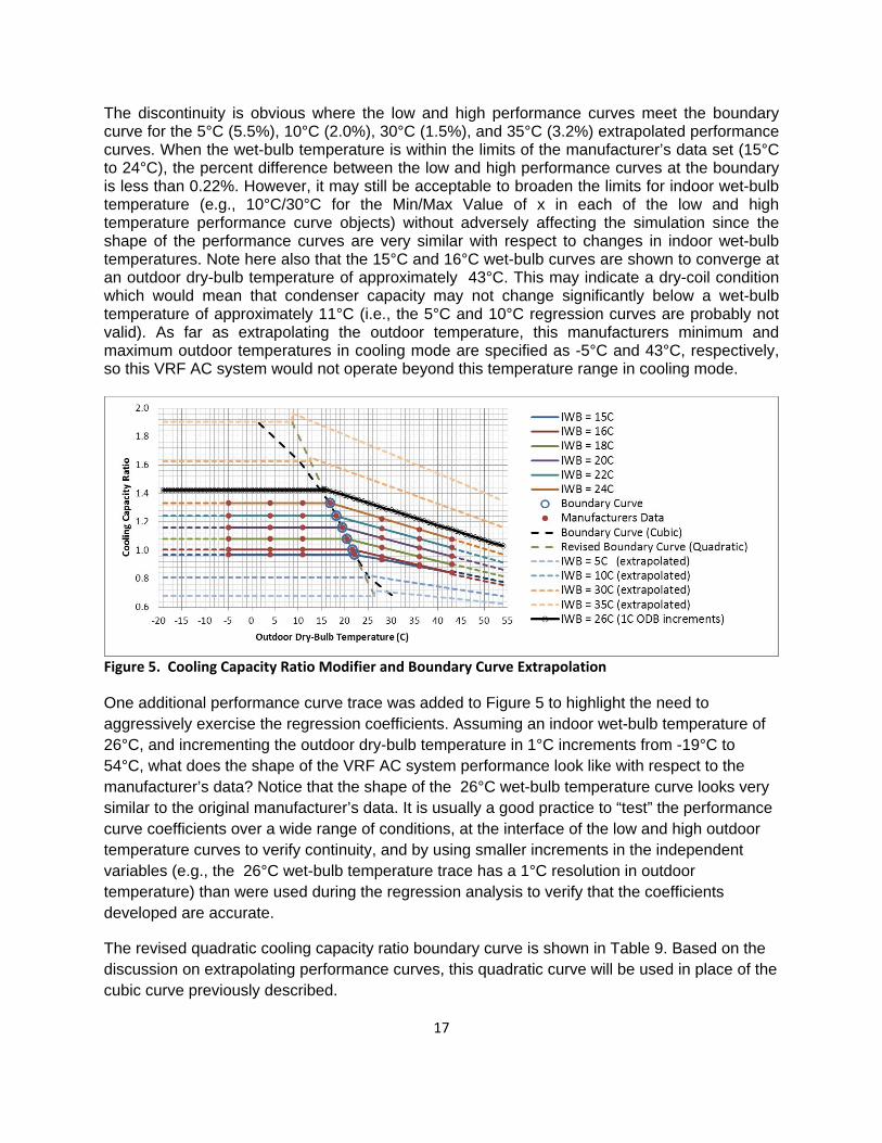
The discontinuity is obvious where the low and high performance curves meet the boundary curve for the 5°C (5.5%), 10°C (2.0%), 30°C (1.5%), and 35°C (3.2%) extrapolated performance curves. When the wet-bulb temperature is within the limits of the manufacturer’s data set (15°C to 24°C), the percent difference between the low and high performance curves at the boundary is less than 0.22%. However, it may still be acceptable to broaden the limits for indoor wet-bulb temperature (e.g., 10°C/30°C for the Min/Max Value of x in each of the low and high temperature performance curve objects) without adversely affecting the simulation since the shape of the performance curves are very similar with respect to changes in indoor wet-bulb temperatures. Note here also that the 15°C and 16°C wet-bulb curves are shown to converge at an outdoor dry-bulb temperature of approximately 43°C. This may indicate a dry-coil condition which would mean that condenser capacity may not change significantly below a wet-bulb temperature of approximately 11°C (i.e., the 5°C and 10°C regression curves are probably not valid). As far as extrapolating the outdoor temperature, this manufacturers minimum and maximum outdoor temperatures in cooling mode are specified as -5°C and 43°C, respectively, so this VRF AC system would not operate beyond this temperature range in cooling mode.

 Figure 5.  Cooling Capacity Ratio Modifier and Boundary Curve Extrapolation 

One additional performance curve trace was added to Figure 5 to highlight the need to aggressively exercise the regression coefficients. Assuming an indoor wet-bulb temperature of 26°C, and incrementing the outdoor dry-bulb temperature in 1°C increments from -19°C to 54°C, what does the shape of the VRF AC system performance look like with respect to the manufacturer’s data? Notice that the shape of the 26°C wet-bulb temperature curve looks very similar to the original manufacturer’s data. It is usually a good practice to “test” the performance curve coefficients over a wide range of conditions, at the interface of the low and high outdoor temperature curves to verify continuity, and by using smaller increments in the independent variables (e.g., the 26°C wet-bulb temperature trace has a 1°C resolution in outdoor temperature) than were used during the regression analysis to verify that the coefficients developed are accurate.

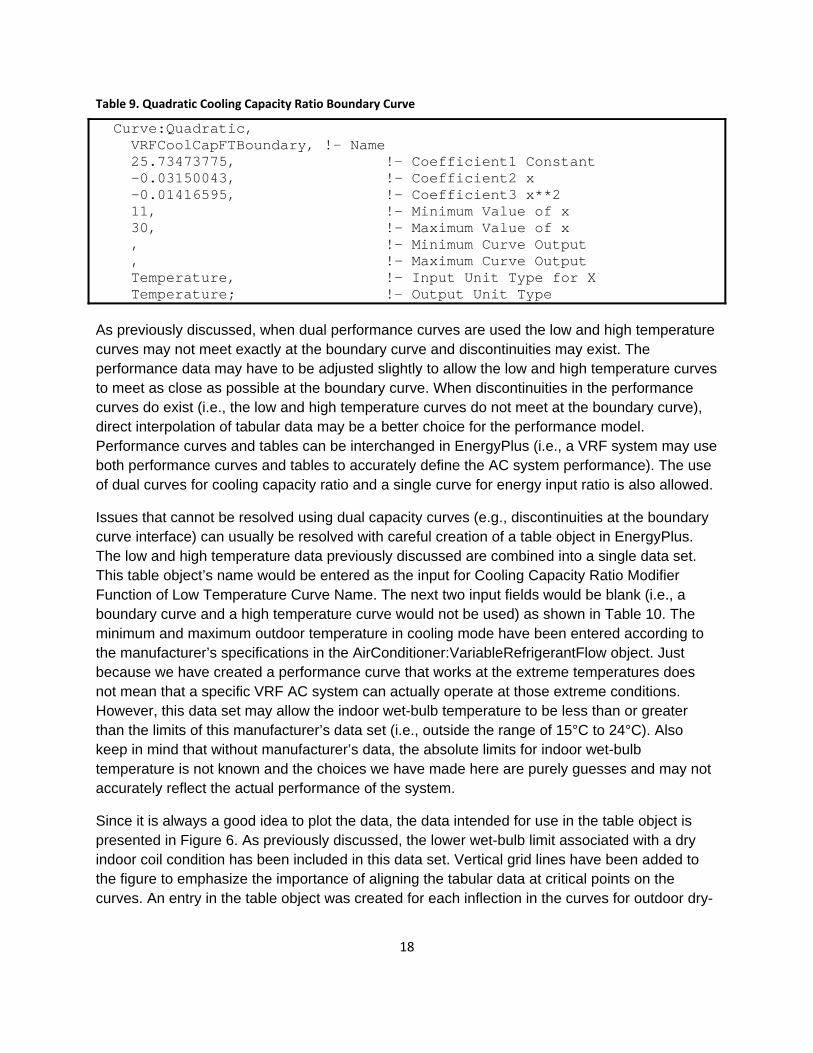
The revised quadratic cooling capacity ratio boundary curve is shown in Table 9. Based on the discussion on extrapolating performance curves, this quadratic curve will be used in place of the cubic curve previously described.

18 

 

Table 9. Quadratic Cooling Capacity Ratio Boundary Curve 

Curve:Quadratic, VRFCoolCapFTBoundary, !- Name 25.73473775, !- Coefficient1 Constant -0.03150043, !- Coefficient2 x -0.01416595, !- Coefficient3 x**2 11, !- Minimum Value of x 30, !- Maximum Value of x , !- Minimum Curve Output , !- Maximum Curve Output Temperature, !- Input Unit Type for X Temperature; !- Output Unit Type As previously discussed, when dual performance curves are used the low and high temperature curves may not meet exactly at the boundary curve and discontinuities may exist. The performance data may have to be adjusted slightly to allow the low and high temperature curves to meet as close as possible at the boundary curve. When discontinuities in the performance curves do exist (i.e., the low and high temperature curves do not meet at the boundary curve), direct interpolation of tabular data may be a better choice for the performance model. Performance curves and tables can be interchanged in EnergyPlus (i.e., a VRF system may use both performance curves and tables to accurately define the AC system performance). The use of dual curves for cooling capacity ratio and a single curve for energy input ratio is also allowed.

Issues that cannot be resolved using dual capacity curves (e.g., discontinuities at the boundary curve interface) can usually be resolved with careful creation of a table object in EnergyPlus. The low and high temperature data previously discussed are combined into a single data set. This table object’s name would be entered as the input for Cooling Capacity Ratio Modifier Function of Low Temperature Curve Name. The next two input fields would be blank (i.e., a boundary curve and a high temperature curve would not be used) as shown in Table 10. The minimum and maximum outdoor temperature in cooling mode have been entered according to the manufacturer’s specifications in the AirConditioner:VariableRefrigerantFlow object. Just because we have created a performance curve that works at the extreme temperatures does not mean that a specific VRF AC system can actually operate at those extreme conditions. However, this data set may allow the indoor wet-bulb temperature to be less than or greater than the limits of this manufacturer’s data set (i.e., outside the range of 15°C to 24°C). Also keep in mind that without manufacturer’s data, the absolute limits for indoor wet-bulb temperature is not known and the choices we have made here are purely guesses and may not accurately reflect the actual performance of the system.

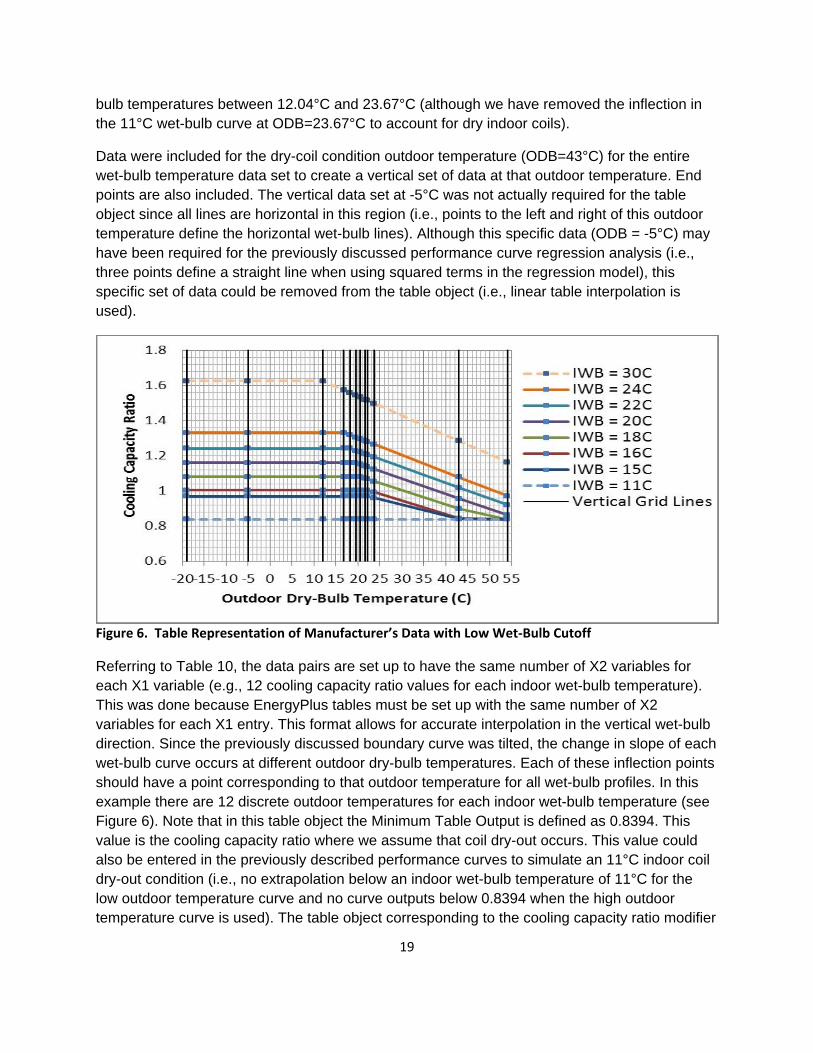
Since it is always a good idea to plot the data, the data intended for use in the table object is presented in Figure 6. As previously discussed, the lower wet-bulb limit associated with a dry indoor coil condition has been included in this data set. Vertical grid lines have been added to the figure to emphasize the importance of aligning the tabular data at critical points on the curves. An entry in the table object was created for each inflection in the curves for outdoor dry-

19 

 

bulb temperatures between 12.04°C and 23.67°C (although we have removed the inflection in the 11°C wet-bulb curve at ODB=23.67°C to account for dry indoor coils).

Data were included for the dry-coil condition outdoor temperature (ODB=43°C) for the entire wet-bulb temperature data set to create a vertical set of data at that outdoor temperature. End points are also included. The vertical data set at -5°C was not actually required for the table object since all lines are horizontal in this region (i.e., points to the left and right of this outdoor temperature define the horizontal wet-bulb lines). Although this specific data (ODB = -5°C) may have been required for the previously discussed performance curve regression analysis (i.e., three points define a straight line when using squared terms in the regression model), this specific set of data could be removed from the table object (i.e., linear table interpolation is used).

Figure 6.  Table Representation of Manufacturer’s Data with Low Wet‐Bulb Cutoff

Referring to Table 10, the data pairs are set up to have the same number of X2 variables for each X1 variable (e.g., 12 cooling capacity ratio values for each indoor wet-bulb temperature). This was done because EnergyPlus tables must be set up with the same number of X2 variables for each X1 entry. This format allows for accurate interpolation in the vertical wet-bulb direction. Since the previously discussed boundary curve was tilted, the change in slope of each wet-bulb curve occurs at different outdoor dry-bulb temperatures. Each of these inflection points should have a point corresponding to that outdoor temperature for all wet-bulb profiles. In this example there are 12 discrete outdoor temperatures for each indoor wet-bulb temperature (see Figure 6). Note that in this table object the Minimum Table Output is defined as 0.8394. This value is the cooling capacity ratio where we assume that coil dry-out occurs. This value could also be entered in the previously described performance curves to simulate an 11°C indoor coil dry-out condition (i.e., no extrapolation below an indoor wet-bulb temperature of 11°C for the low outdoor temperature curve and no curve outputs below 0.8394 when the high outdoor temperature curve is used). The table object corresponding to the cooling capacity ratio modifier

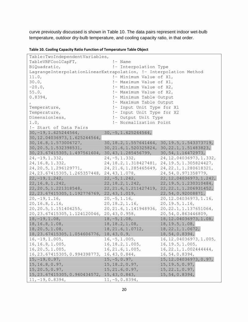
20 

 

curve previously discussed is shown in Table 10. The data pairs represent indoor wet-bulb temperature, outdoor dry-bulb temperature, and cooling capacity ratio, in that order. Table 10. Cooling Capacity Ratio Function of Temperature Table Object 

Table:TwoIndependentVariables, TableVRFCoolCapFT, !- Name BiQuadratic, !- Interpolation Type LagrangeInterpolationLinearExtrapolation, !- Interpolation Method 11.0, !- Minimum Value of X1, 30.0, !- Maximum Value of X1, -20.0, !- Minimum Value of X2, 55.0, !- Maximum Value of X2, 0.8394, !- Minimum Table Output , !- Maximum Table Output Temperature, !- Input Unit Type for X1 Temperature, !- Input Unit Type for X2 Dimensionless, !- Output Unit Type 1.0, !- Normalization Point !- Start of Data Pairs 30,-19,1.625244564, 30,-5,1.625244564, 30,12.04036973,1.625244564, 30,16.8,1.573006727, 30,18.2,1.557641464, 30,19.5,1.543373719, 30,20.5,1.532398531, 30,21.6,1.520325824, 30,22.1,1.51483823, 30,23.67415305,1.497561604, 30,43,1.285456799, 30,54,1.16472973, 24,-19,1.332, 24,-5,1.332, 24,12.04036973,1.332, 24,16.8,1.332, 24,18.2,1.318427481, 24,19.5,1.305824427, 24,20.5,1.296129771, 24,21.6,1.285465649, 24,22.1,1.280618321, 24,23.67415305,1.265357448, 24,43,1.078, 24,54,0.971358779, 22,-19,1.242, 22,-5,1.242, 22,12.04036973,1.242, 22,16.8,1.242, 22,18.2,1.242, 22,19.5,1.230310484, 22,20.5,1.221318548, 22,21.6,1.211427419, 22,22.1,1.206931452, 22,23.67415305,1.192776769, 22,43,1.019, 22,54,0.92008871, 20,-19,1.16, 20,-5,1.16, 20,12.04036973,1.16, 20,16.8,1.16, 20,18.2,1.16, 20,19.5,1.16, 20,20.5,1.151404255, 20,21.6,1.141948936, 20,22.1,1.137651064, 20,23.67415305,1.124120046, 20,43,0.958, 20,54,0.863446809, 18,-19,1.08, 18,-5,1.08, 18,12.04036973,1.08, 18,16.8,1.08, 18,18.2,1.08, 18,19.5,1.08, 18,20.5,1.08, 18,21.6,1.0712, 18,22.1,1.0672, 18,23.67415305,1.054606776, 18,43,0.9, 18,54,0.8394, 16,-19,1.005, 16,-5,1.005, 16,12.04036973,1.005, 16,16.8,1.005, 16,18.2,1.005, 16,19.5,1.005, 16,20.5,1.005, 16,21.6,1.005, 16,22.1,1.002444444, 16,23.67415305,0.994398773, 16,43,0.844, 16,54,0.8394, 15,-19,0.97, 15,-5,0.97, 15,12.04036973,0.97, 15,16.8,0.97, 15,18.2,0.97, 15,19.5,0.97, 15,20.5,0.97, 15,21.6,0.97, 15,22.1,0.97, 15,23.67415305,0.960434572, 15,43,0.843, 15,54,0.8394, 11,-19,0.8394, 11,-5,0.8394,

21 

 

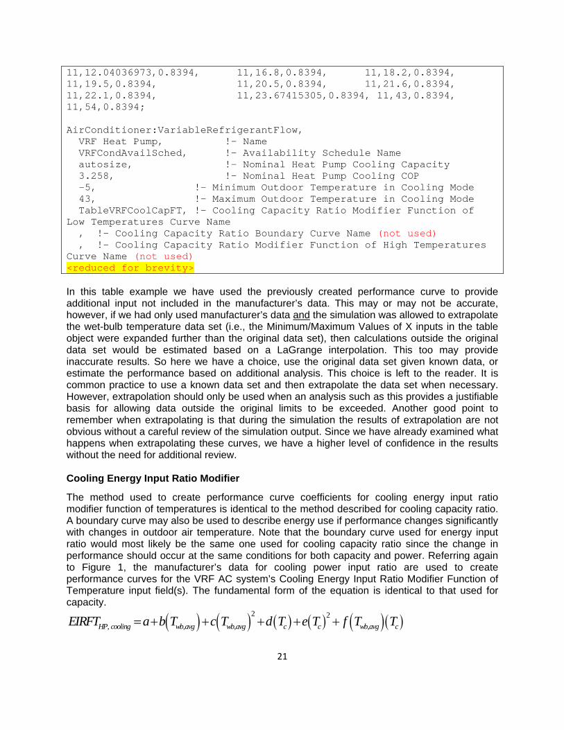
11,12.04036973,0.8394, 11,16.8,0.8394, 11,18.2,0.8394, 11,19.5,0.8394, 11,20.5,0.8394, 11,21.6,0.8394, 11,22.1,0.8394, 11,23.67415305,0.8394, 11,43,0.8394, 11,54,0.8394; AirConditioner:VariableRefrigerantFlow, VRF Heat Pump, !- Name VRFCondAvailSched, !- Availability Schedule Name autosize, !- Nominal Heat Pump Cooling Capacity 3.258, !- Nominal Heat Pump Cooling COP -5, !- Minimum Outdoor Temperature in Cooling Mode 43, !- Maximum Outdoor Temperature in Cooling Mode TableVRFCoolCapFT, !- Cooling Capacity Ratio Modifier Function of Low Temperatures Curve Name , !- Cooling Capacity Ratio Boundary Curve Name (not used) , !- Cooling Capacity Ratio Modifier Function of High Temperatures Curve Name (not used) <reduced for brevity> In this table example we have used the previously created performance curve to provide additional input not included in the manufacturer’s data. This may or may not be accurate, however, if we had only used manufacturer’s data and the simulation was allowed to extrapolate the wet-bulb temperature data set (i.e., the Minimum/Maximum Values of X inputs in the table object were expanded further than the original data set), then calculations outside the original data set would be estimated based on a LaGrange interpolation. This too may provide inaccurate results. So here we have a choice, use the original data set given known data, or estimate the performance based on additional analysis. This choice is left to the reader. It is common practice to use a known data set and then extrapolate the data set when necessary. However, extrapolation should only be used when an analysis such as this provides a justifiable basis for allowing data outside the original limits to be exceeded. Another good point to remember when extrapolating is that during the simulation the results of extrapolation are not obvious without a careful review of the simulation output. Since we have already examined what happens when extrapolating these curves, we have a higher level of confidence in the results without the need for additional review. Cooling Energy Input Ratio Modifier

The method used to create performance curve coefficients for cooling energy input ratio modifier function of temperatures is identical to the method described for cooling capacity ratio. A boundary curve may also be used to describe energy use if performance changes significantly with changes in outdoor air temperature. Note that the boundary curve used for energy input ratio would most likely be the same one used for cooling capacity ratio since the change in performance should occur at the same conditions for both capacity and power. Referring again to Figure 1, the manufacturer’s data for cooling power input ratio are used to create performance curves for the VRF AC system’s Cooling Energy Input Ratio Modifier Function of Temperature input field(s). The fundamental form of the equation is identical to that used for capacity.

2 2

, , , ,HP cooling wb avg wb avg c c wb avg cEIRFT a b T c T d T e T f T T

22 

 

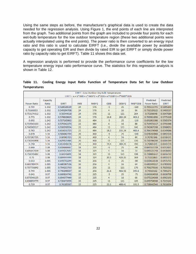
Using the same steps as before, the manufacturer’s graphical data is used to create the data needed for the regression analysis. Using Figure 1, the end points of each line are interpreted from the graph. Two additional points from the graph are included to provide four points for each wet-bulb temperature for the low outdoor temperature region (these two additional points were actually interpolated using the end points). The power ratio is then converted to an energy input ratio and this ratio is used to calculate EIRFT (i.e., divide the available power by available capacity to get operating EIR and then divide by rated EIR to get EIRFT or simply divide power ratio by capacity ratio to get EIRFT). Table 11 shows this data set. A regression analysis is performed to provide the performance curve coefficients for the low temperature energy input ratio performance curve. The statistics for this regression analysis is shown in Table 12. Table  11.    Cooling  Energy  Input  Ratio  Function  of  Temperature  Data  Set  for  Low  Outdoor 

Temperatures 

23 

 

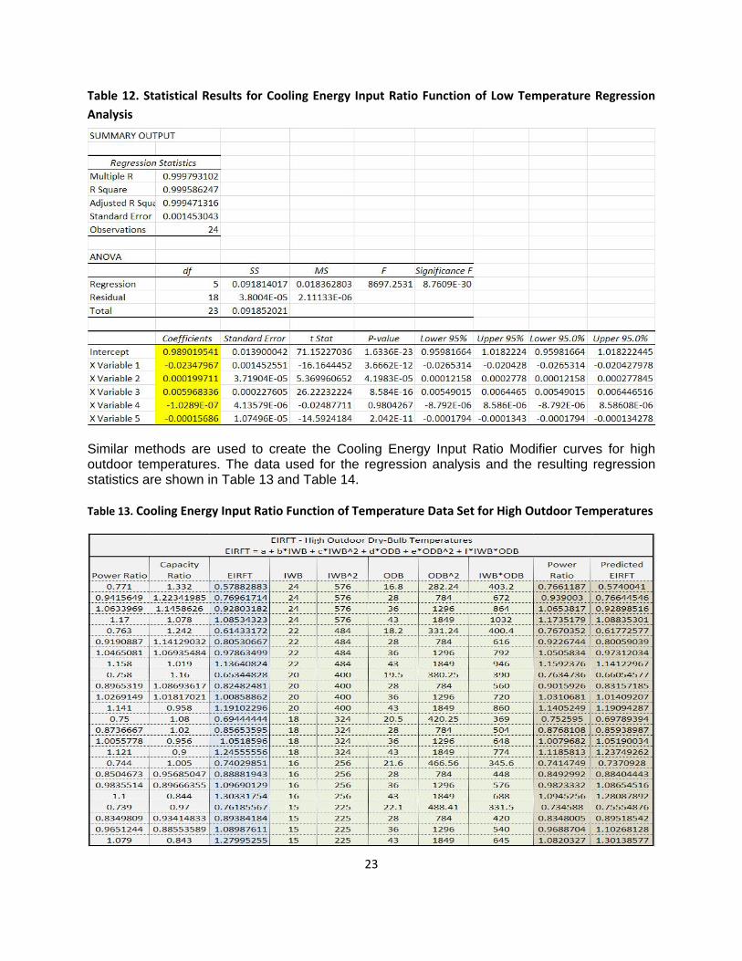
Table 12. Statistical Results  for Cooling Energy  Input Ratio Function of Low Temperature Regression 

Analysis 

  Similar methods are used to create the Cooling Energy Input Ratio Modifier curves for high outdoor temperatures. The data used for the regression analysis and the resulting regression statistics are shown in Table 13 and Table 14. Table 13. Cooling Energy Input Ratio Function of Temperature Data Set for High Outdoor Temperatures 

24 

 

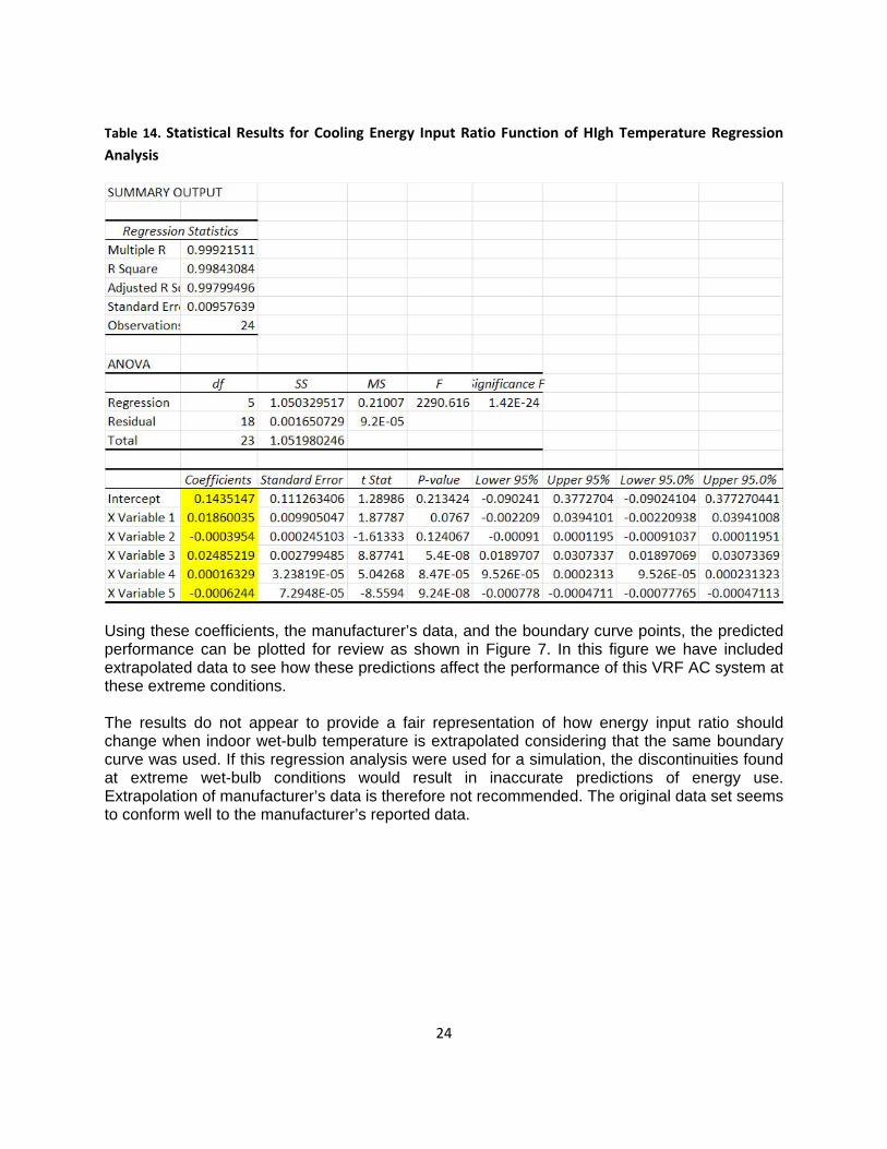
Table 14. Statistical Results  for Cooling Energy  Input Ratio Function of HIgh Temperature Regression 

Analysis 

Using these coefficients, the manufacturer’s data, and the boundary curve points, the predicted performance can be plotted for review as shown in Figure 7. In this figure we have included extrapolated data to see how these predictions affect the performance of this VRF AC system at these extreme conditions. The results do not appear to provide a fair representation of how energy input ratio should change when indoor wet-bulb temperature is extrapolated considering that the same boundary curve was used. If this regression analysis were used for a simulation, the discontinuities found at extreme wet-bulb conditions would result in inaccurate predictions of energy use. Extrapolation of manufacturer’s data is therefore not recommended. The original data set seems to conform well to the manufacturer’s reported data.

25 

 

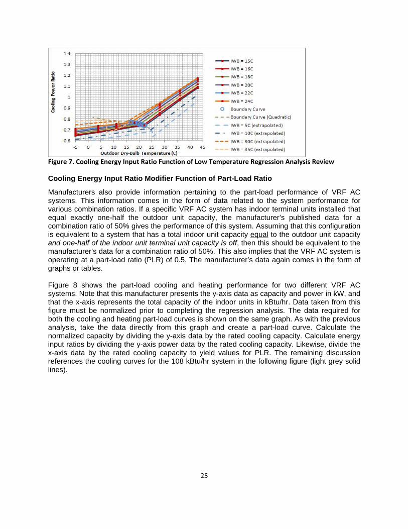
 Figure 7. Cooling Energy Input Ratio Function of Low Temperature Regression Analysis Review 

Cooling Energy Input Ratio Modifier Function of Part-Load Ratio

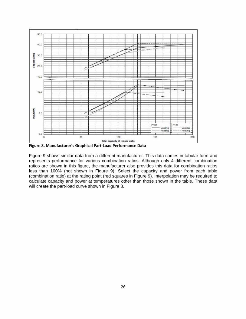
Manufacturers also provide information pertaining to the part-load performance of VRF AC systems. This information comes in the form of data related to the system performance for various combination ratios. If a specific VRF AC system has indoor terminal units installed that equal exactly one-half the outdoor unit capacity, the manufacturer’s published data for a combination ratio of 50% gives the performance of this system. Assuming that this configuration is equivalent to a system that has a total indoor unit capacity equal to the outdoor unit capacity and one-half of the indoor unit terminal unit capacity is off, then this should be equivalent to the manufacturer’s data for a combination ratio of 50%. This also implies that the VRF AC system is operating at a part-load ratio (PLR) of 0.5. The manufacturer’s data again comes in the form of graphs or tables. Figure 8 shows the part-load cooling and heating performance for two different VRF AC systems. Note that this manufacturer presents the y-axis data as capacity and power in kW, and that the x-axis represents the total capacity of the indoor units in kBtu/hr. Data taken from this figure must be normalized prior to completing the regression analysis. The data required for both the cooling and heating part-load curves is shown on the same graph. As with the previous analysis, take the data directly from this graph and create a part-load curve. Calculate the normalized capacity by dividing the y-axis data by the rated cooling capacity. Calculate energy input ratios by dividing the y-axis power data by the rated cooling capacity. Likewise, divide the x-axis data by the rated cooling capacity to yield values for PLR. The remaining discussion references the cooling curves for the 108 kBtu/hr system in the following figure (light grey solid lines).

26 

 

 Figure 8. Manufacturer’s Graphical Part‐Load Performance Data

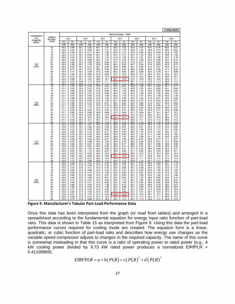
Figure 9 shows similar data from a different manufacturer. This data comes in tabular form and represents performance for various combination ratios. Although only 4 different combination ratios are shown in this figure, the manufacturer also provides this data for combination ratios less than 100% (not shown in Figure 9). Select the capacity and power from each table (combination ratio) at the rating point (red squares in Figure 9). Interpolation may be required to calculate capacity and power at temperatures other than those shown in the table. These data will create the part-load curve shown in Figure 8.

27 

 

 Figure 9. Manufacturer’s Tabular Part‐Load Performance Data 

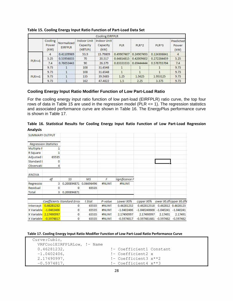
Once this data has been interpreted from the graph (or read from tables) and arranged in a spreadsheet according to the fundamental equation for energy input ratio function of part-load ratio. This data is shown in Table 15 as interpreted from Figure 9. Using this data the part-load performance curves required for cooling mode are created. The equation form is a linear, quadratic, or cubic function of part-load ratio and describes how energy use changes as the variable speed compressor adjusts to changes in the required capacity. The name of this curve is somewhat misleading in that this curve is a ratio of operating power to rated power (e.g., 4 kW cooling power divided by 9.73 kW rated power produces a normalized EIRfPLR = 0.41109969).

2 3EIRFPLR a b PLR c PLR d PLR

28 

 

Table 15. Cooling Energy Input Ratio Function of Part‐Load Data Set 

  Cooling Energy Input Ratio Modifier Function of Low Part-Load Ratio

For the cooling energy input ratio function of low part-load (EIRFPLR) ratio curve, the top four rows of data in Table 15 are used in the regression model (PLR <= 1). The regression statistics and associated performance curve are shown in Table 16. The EnergyPlus performance curve is shown in Table 17.  Table  16.  Statistical  Results  for  Cooling  Energy  Input  Ratio  Function  of  Low  Part‐Load  Regression 

Analysis 

   Table 17. Cooling Energy Input Ratio Modifier Function of Low Part‐Load Ratio Performance Curve 

Curve:Cubic, VRFCoolEIRFPLRLow, !- Name 0.46281232, !- Coefficient1 Constant -1.0402406, !- Coefficient2 x 2.17490997, !- Coefficient3 x**2 -0.5974817, !- Coefficient4 x**3

29 

 

0, !- Minimum Value of x 1, !- Maximum Value of x , !- Minimum Curve Output , !- Maximum Curve Output Dimensionless, !- Input Unit Type for X Dimensionless; !- Output Unit Type Cooling Energy Input Ratio Modifier Function of High Part-Load Ratio

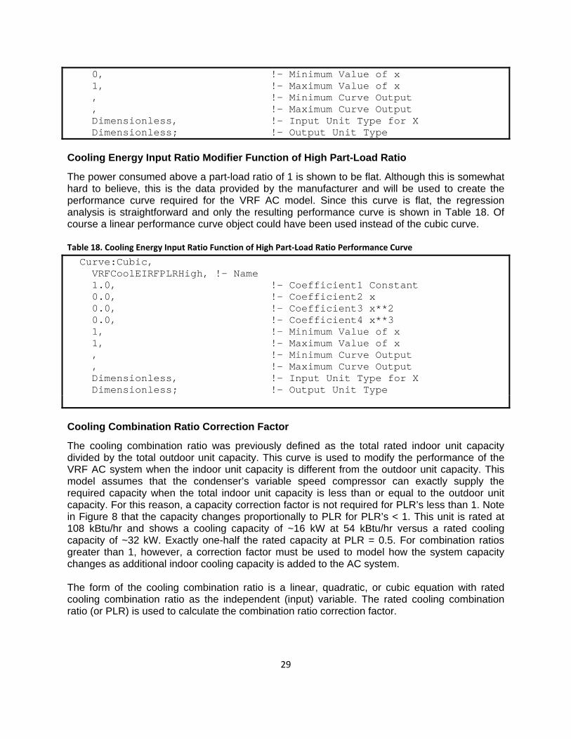
The power consumed above a part-load ratio of 1 is shown to be flat. Although this is somewhat hard to believe, this is the data provided by the manufacturer and will be used to create the performance curve required for the VRF AC model. Since this curve is flat, the regression analysis is straightforward and only the resulting performance curve is shown in Table 18. Of course a linear performance curve object could have been used instead of the cubic curve. Table 18. Cooling Energy Input Ratio Function of High Part‐Load Ratio Performance Curve 

Curve:Cubic, VRFCoolEIRFPLRHigh, !- Name 1.0, !- Coefficient1 Constant 0.0, !- Coefficient2 x 0.0, !- Coefficient3 x**2 0.0, !- Coefficient4 x**3 1, !- Minimum Value of x 1, !- Maximum Value of x , !- Minimum Curve Output , !- Maximum Curve Output Dimensionless, !- Input Unit Type for X Dimensionless; !- Output Unit Type Cooling Combination Ratio Correction Factor

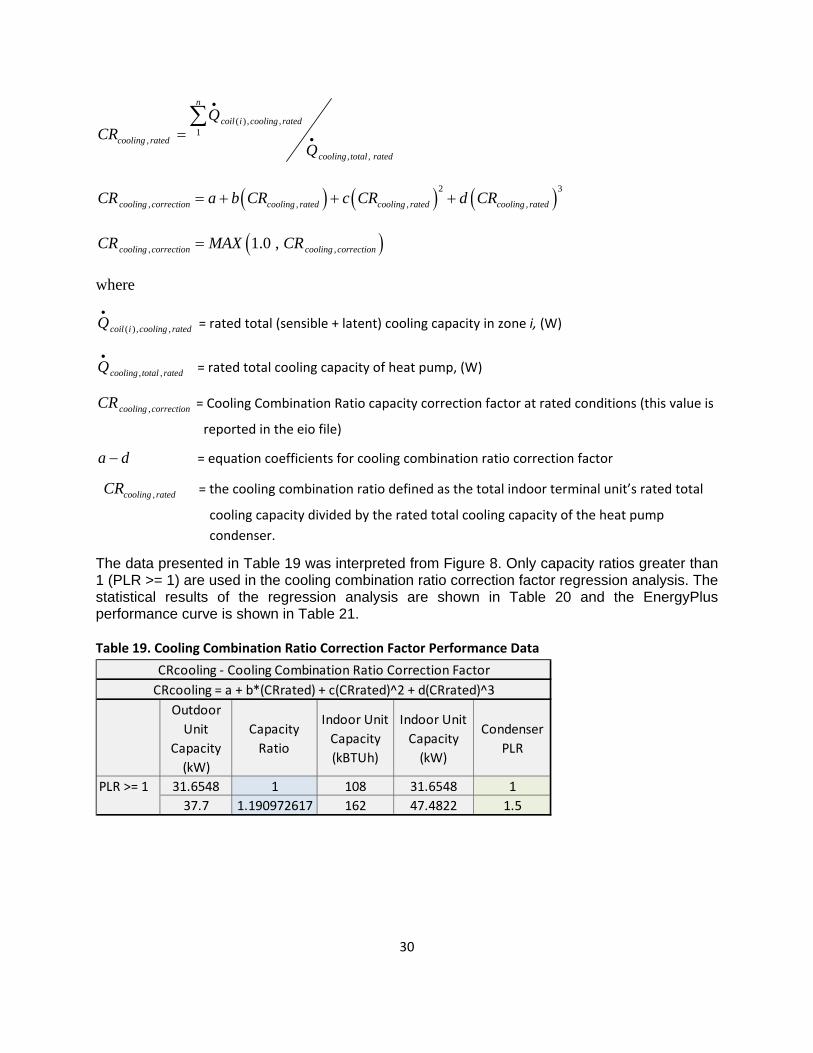
The cooling combination ratio was previously defined as the total rated indoor unit capacity divided by the total outdoor unit capacity. This curve is used to modify the performance of the VRF AC system when the indoor unit capacity is different from the outdoor unit capacity. This model assumes that the condenser’s variable speed compressor can exactly supply the required capacity when the total indoor unit capacity is less than or equal to the outdoor unit capacity. For this reason, a capacity correction factor is not required for PLR’s less than 1. Note in Figure 8 that the capacity changes proportionally to PLR for PLR’s < 1. This unit is rated at 108 kBtu/hr and shows a cooling capacity of ~16 kW at 54 kBtu/hr versus a rated cooling capacity of ~32 kW. Exactly one-half the rated capacity at PLR = 0.5. For combination ratios greater than 1, however, a correction factor must be used to model how the system capacity changes as additional indoor cooling capacity is added to the AC system. The form of the cooling combination ratio is a linear, quadratic, or cubic equation with rated cooling combination ratio as the independent (input) variable. The rated cooling combination ratio (or PLR) is used to calculate the combination ratio correction factor.

30 

 

( ) , ,1

,

, ,

n

coil i cooling rated

cooling rated

cooling total rated

QCR

Q

 

2 3

, , , ,cooling correction cooling rated cooling rated cooling ratedCR a b CR c CR d CR  

, ,1.0 ,cooling correction cooling correctionCR MAX CR  

where

( ), ,coil i cooling ratedQ

 = rated total (sensible + latent) cooling capacity in zone i, (W) 

, ,cooling total ratedQ

   = rated total cooling capacity of heat pump, (W) 

,cooling correctionCR  = Cooling Combination Ratio capacity correction factor at rated conditions (this value is 

reported in the eio file) 

a d    = equation coefficients for cooling combination ratio correction factor 

,cooling ratedCR       = the cooling combination ratio defined as the total indoor terminal unit’s rated total 

cooling capacity divided by the rated total cooling capacity of the heat pump 

condenser. 

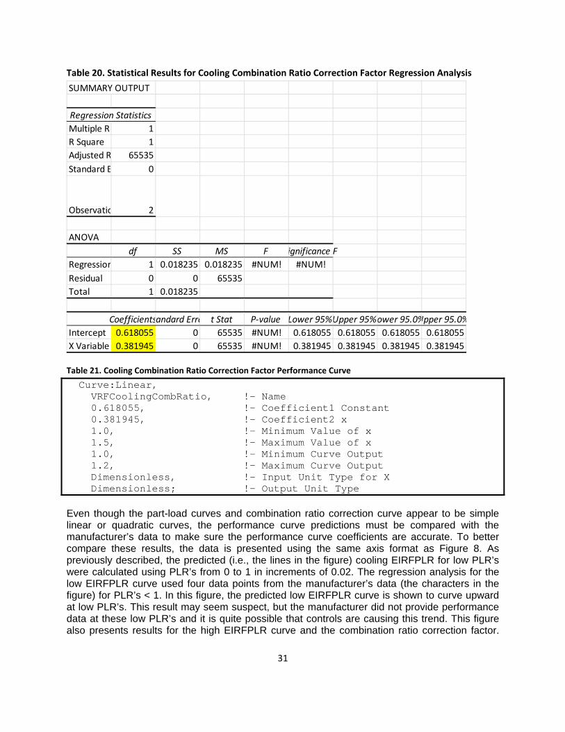
The data presented in Table 19 was interpreted from Figure 8. Only capacity ratios greater than 1 (PLR >= 1) are used in the cooling combination ratio correction factor regression analysis. The statistical results of the regression analysis are shown in Table 20 and the EnergyPlus performance curve is shown in Table 21. Table 19. Cooling Combination Ratio Correction Factor Performance Data 

Outdoor 

Unit 

Capacity 

(kW)

Capacity 

Ratio

Indoor Unit 

Capacity 

(kBTUh)

Indoor Unit 

Capacity 

(kW)

Condenser 

PLR

PLR >= 1 31.6548 1 108 31.6548 1

37.7 1.190972617 162 47.4822 1.5

CRcooling = a + b*(CRrated) + c(CRrated)^2 + d(CRrated)^3

CRcooling ‐ Cooling Combination Ratio Correction Factor

 

31 

 

Table 20. Statistical Results for Cooling Combination Ratio Correction Factor Regression Analysis 

SUMMARY OUTPUT

Regression Statistics

Multiple R 1

R Square 1

Adjusted R 65535

Standard E 0

Observatio 2

ANOVA

df SS MS F ignificance F

Regression 1 0.018235 0.018235 #NUM! #NUM!

Residual 0 0 65535

Total 1 0.018235

Coefficientstandard Erro t Stat P‐value Lower 95%Upper 95%ower 95.0%Upper 95.0%

Intercept 0.618055 0 65535 #NUM! 0.618055 0.618055 0.618055 0.618055

X Variable  0.381945 0 65535 #NUM! 0.381945 0.381945 0.381945 0.381945   Table 21. Cooling Combination Ratio Correction Factor Performance Curve 

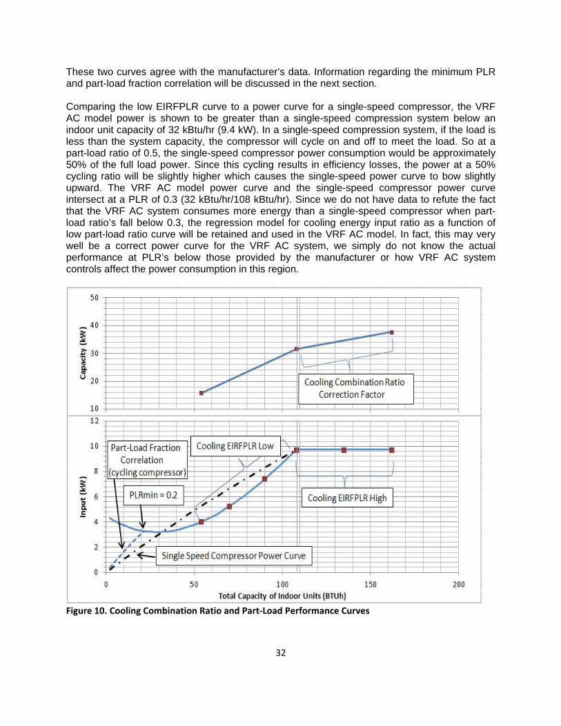
Curve:Linear, VRFCoolingCombRatio, !- Name 0.618055, !- Coefficient1 Constant 0.381945, !- Coefficient2 x 1.0, !- Minimum Value of x 1.5, !- Maximum Value of x 1.0, !- Minimum Curve Output 1.2, !- Maximum Curve Output Dimensionless, !- Input Unit Type for X Dimensionless; !- Output Unit Type Even though the part-load curves and combination ratio correction curve appear to be simple linear or quadratic curves, the performance curve predictions must be compared with the manufacturer’s data to make sure the performance curve coefficients are accurate. To better compare these results, the data is presented using the same axis format as Figure 8. As previously described, the predicted (i.e., the lines in the figure) cooling EIRFPLR for low PLR’s were calculated using PLR’s from 0 to 1 in increments of 0.02. The regression analysis for the low EIRFPLR curve used four data points from the manufacturer’s data (the characters in the figure) for PLR’s < 1. In this figure, the predicted low EIRFPLR curve is shown to curve upward at low PLR’s. This result may seem suspect, but the manufacturer did not provide performance data at these low PLR’s and it is quite possible that controls are causing this trend. This figure also presents results for the high EIRFPLR curve and the combination ratio correction factor.

32 

 

These two curves agree with the manufacturer’s data. Information regarding the minimum PLR and part-load fraction correlation will be discussed in the next section. Comparing the low EIRFPLR curve to a power curve for a single-speed compressor, the VRF AC model power is shown to be greater than a single-speed compression system below an indoor unit capacity of 32 kBtu/hr (9.4 kW). In a single-speed compression system, if the load is less than the system capacity, the compressor will cycle on and off to meet the load. So at a part-load ratio of 0.5, the single-speed compressor power consumption would be approximately 50% of the full load power. Since this cycling results in efficiency losses, the power at a 50% cycling ratio will be slightly higher which causes the single-speed power curve to bow slightly upward. The VRF AC model power curve and the single-speed compressor power curve intersect at a PLR of 0.3 (32 kBtu/hr/108 kBtu/hr). Since we do not have data to refute the fact that the VRF AC system consumes more energy than a single-speed compressor when part-load ratio’s fall below 0.3, the regression model for cooling energy input ratio as a function of low part-load ratio curve will be retained and used in the VRF AC model. In fact, this may very well be a correct power curve for the VRF AC system, we simply do not know the actual performance at PLR’s below those provided by the manufacturer or how VRF AC system controls affect the power consumption in this region.

 Figure 10. Cooling Combination Ratio and Part‐Load Performance Curves

33 

 

Cooling Part-Load Fraction Correlation Curve

Variable speed compressors do have a minimum PLR below which the compressor cycles to meet the load. To calculate the performance for cycling compressors, a compressor part-load fraction (PLF) correlation is used to determine cycling losses. When a compressor turns on, the capacity provided does not immediately increase to the desired capacity. There is some time required to reach the steady-state capacity. The cooling part-load fraction correlation curve defines these startup losses. Figure 10 shows an assumed minimum PLR of 0.2 (the manufacturer’s minimum PLR may reasonably be between 0.4 and 0.1). At this point on the low EIRFPLR curve, the compressor will start to cycle. The cycling rate at this point is 1 and the power consumption is 3.3 kW. The part-load fraction correlation defines the energy required to overcome startup losses as the compressor cycles on and off. Below a PLR of 0.2, when the compressor is on, the power consumption is 3.3 kW. When the compressor is off, the power consumption is 0. The part-load fraction correlation curve is used to determine the power consumption for any compressor cycling rate between a system PLR of 0 and 0.2. The dotted line in the figure from 3.3 kW to 0 kW shows how the part-load fraction correlation is applied to the VRF AC model. When the operating PLR is less than the minimum PLR, the VRF AC model will ride this curve (the dotted line). A typical part-load fraction correlation is shown in Table 22. Manufacturers do not typically provide information regarding cycling losses and this part of the VRF AC model uses standard loss curves for single-speed compression systems. This aspect of performance is usually measured in a laboratory. The mathematical derivation is analogous to the degradation coefficient (CD) used for direct expansion (DX) equipment. Below the minimum PLR (see Figure 10), the power use is proportional to the runtime fraction (RTF) of the cycling compressor.

, 1, coolingcooling cycling

minPLR

PLRPLR MIN PLR

,cooling cycling

cooling

PLRRuntime Fraction PLF

,cooling cycling minPLRP P Runtime Fraction

Table 22. Cooling Part‐Load Fraction Correlation Performance Curve 

Curve:Linear, VRFCoolingPLF, !- Name 0.85, !- Coefficient1 Constant 0.15, !- Coefficient2 x 0.0, !- Minimum Value of x 1.0, !- Maximum Value of x 0.85, !- Minimum Curve Output 1.0, !- Maximum Curve Output Dimensionless, !- Input Unit Type for X Dimensionless; !- Output Unit Type

34 

 

Piping Correction Factors

Variable refrigerant flow air conditioning systems connect the outdoor condenser to the indoor terminal units through refrigerant lines. These refrigerant lines can vary in length based on the specific configuration of the system. Inputs to the VRF AC model include a length and height in meters to define the system layout. A piping correction factor for length in cooling mode curve is used to determine the piping losses based on the length of the refrigerant lines. A coefficient is also used to determine the piping losses due to a height difference between the terminal units and the outdoor condenser. If the terminal units are all above (or below) the outdoor condenser, then the height is simply the highest (or lowest) terminal unit. If there are terminal units above and below the outdoor condenser, then the height used in this model is the difference between the highest and lowest terminal unit (e.g., 10 m above – 2 m below = 8 m or 2 m above - 10 m below = -8 m). Piping Correction Factor for Length in Cooling Mode

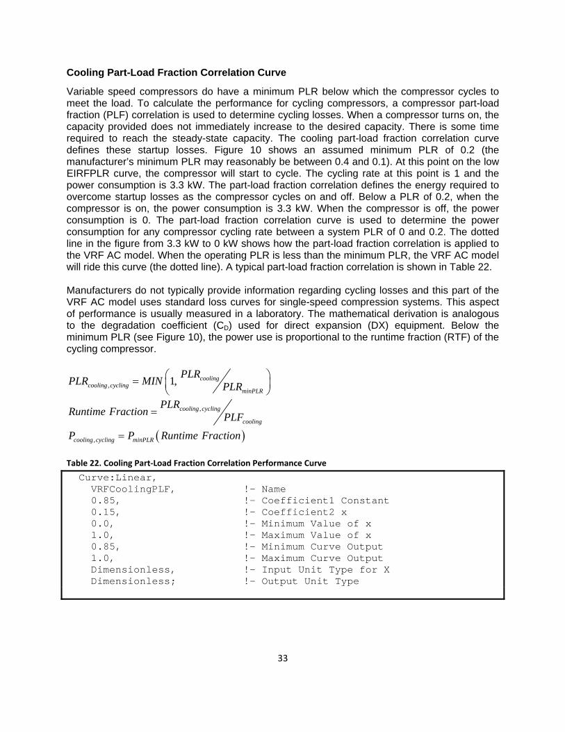
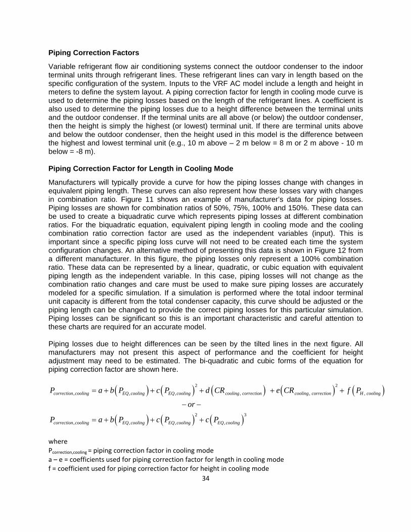
Manufacturers will typically provide a curve for how the piping losses change with changes in equivalent piping length. These curves can also represent how these losses vary with changes in combination ratio. Figure 11 shows an example of manufacturer’s data for piping losses. Piping losses are shown for combination ratios of 50%, 75%, 100% and 150%. These data can be used to create a biquadratic curve which represents piping losses at different combination ratios. For the biquadratic equation, equivalent piping length in cooling mode and the cooling combination ratio correction factor are used as the independent variables (input). This is important since a specific piping loss curve will not need to be created each time the system configuration changes. An alternative method of presenting this data is shown in Figure 12 from a different manufacturer. In this figure, the piping losses only represent a 100% combination ratio. These data can be represented by a linear, quadratic, or cubic equation with equivalent piping length as the independent variable. In this case, piping losses will not change as the combination ratio changes and care must be used to make sure piping losses are accurately modeled for a specific simulation. If a simulation is performed where the total indoor terminal unit capacity is different from the total condenser capacity, this curve should be adjusted or the piping length can be changed to provide the correct piping losses for this particular simulation. Piping losses can be significant so this is an important characteristic and careful attention to these charts are required for an accurate model. Piping losses due to height differences can be seen by the tilted lines in the next figure. All manufacturers may not present this aspect of performance and the coefficient for height adjustment may need to be estimated. The bi-quadratic and cubic forms of the equation for piping correction factor are shown here.

2 2

, , , , , ,

2 3

, , , ,

correction cooling EQ cooling EQ cooling cooling correction cooling correction H cooling

correction cooling EQ cooling EQ cooling EQ cooling

P a b P c P d CR e CR f P

or

P a b P c P c P

 where Pcorrection,cooling = piping correction factor in cooling mode a – e = coefficients used for piping correction factor for length in cooling mode f = coefficient used for piping correction factor for height in cooling mode 

35 

 

PEQ,cooling = equivalent piping length in cooling mode (m) CRcooling, correction = combination ratio correction factor in cooling mode 

PH,cooling = piping height in cooling mode (m)  

 Figure 11. Manufacturer A Cooling Capacity Correction Factor for Piping Length

 Figure 12. Manufacturer B Cooling Capacity Correction Factor for Piping Length

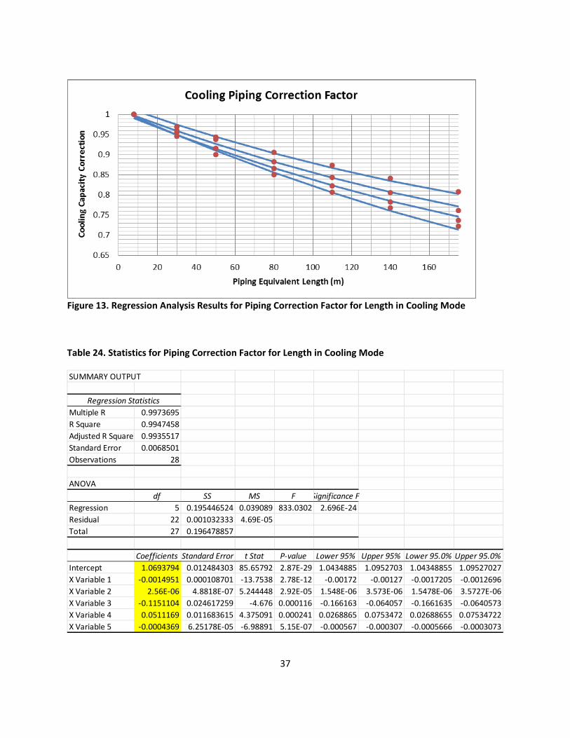
Using this information a regression analysis can be performed based on the piping losses per unit length of the refrigerant lines. Interpreting data from Figure 11 provides the information required to create the piping correction factor for length in cooling mode performance curve coefficients. The predicted cooling piping correction factor is compared to the manufacturer’s data in Figure 13. Although the R-square value for this regression model is 99.47%, the predicted piping losses do not accurately line up with the manufacturer’s data. At the minimum refrigerant line length, the predicted lines do not pass through the same point. This is comment when biquadratic regression models are used. This specific point could be weighted by adding more rows in Table 23 where these lines cross at 1. This has a tendency to “pull” the regression model towards that point since the regression analysis attempts to minimize the residuals for all

36 

 

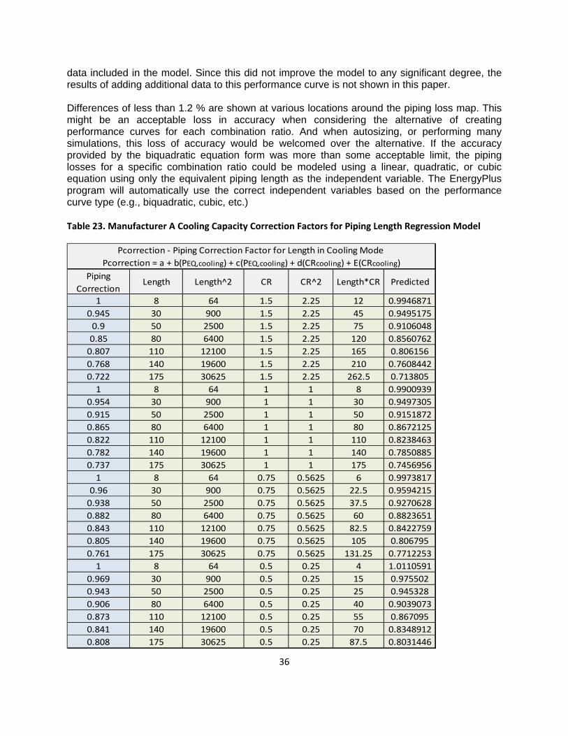
data included in the model. Since this did not improve the model to any significant degree, the results of adding additional data to this performance curve is not shown in this paper. Differences of less than 1.2 % are shown at various locations around the piping loss map. This might be an acceptable loss in accuracy when considering the alternative of creating performance curves for each combination ratio. And when autosizing, or performing many simulations, this loss of accuracy would be welcomed over the alternative. If the accuracy provided by the biquadratic equation form was more than some acceptable limit, the piping losses for a specific combination ratio could be modeled using a linear, quadratic, or cubic equation using only the equivalent piping length as the independent variable. The EnergyPlus program will automatically use the correct independent variables based on the performance curve type (e.g., biquadratic, cubic, etc.) Table 23. Manufacturer A Cooling Capacity Correction Factors for Piping Length Regression Model 

Piping 

CorrectionLength Length^2 CR CR^2 Length*CR Predicted

1 8 64 1.5 2.25 12 0.9946871

0.945 30 900 1.5 2.25 45 0.9495175

0.9 50 2500 1.5 2.25 75 0.9106048

0.85 80 6400 1.5 2.25 120 0.8560762

0.807 110 12100 1.5 2.25 165 0.806156

0.768 140 19600 1.5 2.25 210 0.7608442

0.722 175 30625 1.5 2.25 262.5 0.713805

1 8 64 1 1 8 0.9900939

0.954 30 900 1 1 30 0.9497305

0.915 50 2500 1 1 50 0.9151872

0.865 80 6400 1 1 80 0.8672125

0.822 110 12100 1 1 110 0.8238463

0.782 140 19600 1 1 140 0.7850885

0.737 175 30625 1 1 175 0.7456956

1 8 64 0.75 0.5625 6 0.9973817

0.96 30 900 0.75 0.5625 22.5 0.9594215

0.938 50 2500 0.75 0.5625 37.5 0.9270628

0.882 80 6400 0.75 0.5625 60 0.8823651

0.843 110 12100 0.75 0.5625 82.5 0.8422759

0.805 140 19600 0.75 0.5625 105 0.806795

0.761 175 30625 0.75 0.5625 131.25 0.7712253

1 8 64 0.5 0.25 4 1.0110591

0.969 30 900 0.5 0.25 15 0.975502

0.943 50 2500 0.5 0.25 25 0.945328

0.906 80 6400 0.5 0.25 40 0.9039073

0.873 110 12100 0.5 0.25 55 0.867095

0.841 140 19600 0.5 0.25 70 0.8348912

0.808 175 30625 0.5 0.25 87.5 0.8031446

Pcorrection ‐ Piping Correction Factor for Length in Cooling Mode 

Pcorrection = a + b(PEQ,cooling) + c(PEQ,cooling) + d(CRcooling) + E(CRcooling)

 

37 

 

 

 Figure 13. Regression Analysis Results for Piping Correction Factor for Length in Cooling Mode 

Table 24. Statistics for Piping Correction Factor for Length in Cooling Mode 

SUMMARY OUTPUT

Regression Statistics

Multiple R 0.9973695

R Square 0.9947458

Adjusted R Square 0.9935517

Standard Error 0.0068501

Observations 28

ANOVA

df SS MS F Significance F

Regression 5 0.195446524 0.039089 833.0302 2.696E‐24

Residual 22 0.001032333 4.69E‐05

Total 27 0.196478857

Coefficients Standard Error t Stat P‐value Lower 95% Upper 95% Lower 95.0% Upper 95.0%

Intercept 1.0693794 0.012484303 85.65792 2.87E‐29 1.0434885 1.0952703 1.04348855 1.09527027

X Variable 1 ‐0.0014951 0.000108701 ‐13.7538 2.78E‐12 ‐0.00172 ‐0.00127 ‐0.0017205 ‐0.0012696

X Variable 2 2.56E‐06 4.8818E‐07 5.244448 2.92E‐05 1.548E‐06 3.573E‐06 1.5478E‐06 3.5727E‐06

X Variable 3 ‐0.1151104 0.024617259 ‐4.676 0.000116 ‐0.166163 ‐0.064057 ‐0.1661635 ‐0.0640573

X Variable 4 0.0511169 0.011683615 4.375091 0.000241 0.0268865 0.0753472 0.02688655 0.07534722

X Variable 5 ‐0.0004369 6.25178E‐05 ‐6.98891 5.15E‐07 ‐0.000567 ‐0.000307 ‐0.0005666 ‐0.0003073

38 

 

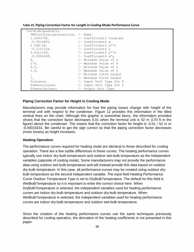
Table 25. Piping Correction Factor for Length in Cooling Mode Performance Curve 

Curve:Biquadratic, VRFCoolPipingCorrection, !- Name 1.0693794, !- Coefficient1 Constant -0.0014951, !- Coefficient2 x 2.56E-06, !- Coefficient3 x**2 -0.1151104, !- Coefficient4 y 0.0511169, !- Coefficient5 y**2 -0.0004369, !- Coefficient6 x*y 8, !- Minimum Value of x 175, !- Maximum Value of x 0.5, !- Minimum Value of y 1.5, !- Maximum Value of y , !- Minimum Curve Output 1, !- Maximum Curve Output Distance, !- Input Unit Type for X Dimensionless, !- Input Unit Type for Y Dimensionless; !- Output Unit Type

Piping Correction Factor for Height in Cooling Mode

Manufacturers may provide information for how the piping losses change with height of the terminal unit with respect to the condenser. Figure 12 provides this information in the tilted vertical lines on the chart. Although this graphic is somewhat blurry, the information provided shows that the correction factor decreases 0.01 when the terminal unit is 52 m (170 ft in the figure) above the condenser. The means that the correction factor for height is -0.01 / 52 m or -0.00019231. Be careful to get the sign correct so that the piping correction factor decreases (more losses) as height increases. Heating Operation

The performance curves required for heating mode are identical to those described for cooling operation. There are a few subtle differences in these curves. The heating performance curves typically use indoor dry-bulb temperature and outdoor wet-bulb temperature as the independent variables (opposite of cooling mode). Some manufacturers may not provide the performance data using outdoor wet-bulb temperature and will instead provide this data based on outdoor dry-bulb temperature. In this case, all performance curves may be created using outdoor dry-bulb temperature as the second independent variable. The input field Heating Performance Curve Outdoor Temperature Type is set to DryBulbTemperature. The default for this field is WetBulbTemperature so it is important to enter the correct choice here. When DryBulbTemperature is selected, the independent variables used for heating performance curves are indoor dry-bulb temperature and outdoor dry-bulb temperature. When WetBulbTemperature is selected, the independent variables used for heating performance curves are indoor dry-bulb temperature and outdoor wet-bulb temperature.

Since the creation of the heating performance curves use the same techniques previously described for cooling operation, the derivation of the heating coefficients is not presented in this paper.