CRANFIELD UNIVERSITY Gang Zhao Individual Research Project ... · PDF fileCRANFIELD UNIVERSITY...
190
CRANFIELD UNIVERSITY Gang Zhao Individual Research Project Report School of Applied Science Advanced Bearing System for Ultra Precision Plastic Electronics Production Systems Academic Year: 2013 - 2014 Supervisor: Paul Shore & Paul Morantz September 2014
Transcript of CRANFIELD UNIVERSITY Gang Zhao Individual Research Project ... · PDF fileCRANFIELD UNIVERSITY...

CRANFIELD UNIVERSITY
Gang Zhao
Individual Research Project Report
School of Applied Science
Advanced Bearing System for Ultra Precision Plastic Electronics
Production Systems
Academic Year: 2013 - 2014
Supervisor: Paul Shore & Paul Morantz
September 2014

CRANFIELD UNIVERSITY
School of Applied Science
Advanced Bearing System for Ultra Precision Plastic Electronics
Production Systems
Academic Year 2013 - 2014
Gang Zhao
Individual Research Project Report
Supervisor: Paul Shore & Paul Morantz
September 2014
© Cranfield University 2014. All rights reserved. No part of this
publication may be reproduced without the written permission of the
copyright owner.

ABSTRACT
The aims of this MSc research project are to investigate the application of
aluminium for the main components of an ultra-precision spindle defined for use
in R2R production systems and to produce a reel to reel rotary aluminium
hydrostatic bearing system of high accuracy to meet the demand of
manufacturing the flexible displays with an effective production capability for this
special kind of film-based product.
The original concept design was already finished to manufacture the bearing
components and the objective of this project was to test the functionality of this
new hydrostatic bearing system. Firstly, theoretical were performed to work out
the output responses, including temperature rise, flow rate, load capacity etc., of
the hydrostatic bearing system under different input design parameters,
including supply pressure, fluid viscosity, the rotational speed etc. Then ANSYS
software was used to build a FEA model to simulate the actual working
conditions of the hydrostatic bearing system and to obtain the theoretical output
parameters, especially the deflection conditions of the bearing shaft. Finally the
experimental validation tests were conducted to verify the actual output
responses to check correlation with the modelled results.
Keywords: R2R production systems, hydrostatic bearing systems, input
parameters, output responses, FEA modelling, deflection conditions of the
bearing shaft.


ACKNOWLEDGEMENTS
Many sincere thanks to the valuable mentorship from my two supervisors,
Professor Paul Shore and Mr Paul Morantz as well as the instructions from the
Subject adviser, Dr Xavier Tonnellier.
Many thanks to the help and assistance from Mr Rodger Read, Mr Keith Carlisle,
Mr Renaud Jourdain, and all the technicians in the Ultra-precision laboratory, Mr
Alan Heaume, Mr Adam Kerr, Mr Kevin Howard and Mr John Hedge.


TABLE OF CONTENTS
ABSTRACT ......................................................................................................... i
ACKNOWLEDGEMENTS................................................................................... iii
LIST OF FIGURES ............................................................................................ vii
LIST OF TABLES .............................................................................................. xii
LIST OF EQUATIONS ...................................................................................... xvi
LIST OF ABBREVIATIONS ............................................................................ xviii
1 INTRODUCTION ............................................................................................. 1
1.1 BACKGROUND ........................................................................................ 1
1.1.1 INTRODUCTION TO PLASTIC ELECTRONICS PRODUCTION
SYSTEMS ................................................................................................... 1
1.1.2 THE CHARACTERISTICS OF THE HYDROSTATIC BEARINGS ..... 1
1.1.3 THE APPLICATIONS OF THE HYDROSTATIC BEARINGS ............. 1
1.2 THE PROJECT PLAN ............................................................................... 1
1.3 GANTT CHART OF THE IRP PLAN ......................................................... 1
1.4 AIMS AND OBJECTIVES ......................................................................... 3
2 LITERATURE REVIEW ................................................................................... 5
2.1 ASSUMPTIONS ........................................................................................ 5
2.2 REVIEW OF THE THEORETICAL DESIGN APPLIED TO ULTRA-
PRECISION SPINDLE .................................................................................... 9
3 DESIGN OF SPINDLE SYSTEM ................................................................... 25
3.1 THE INITIAL DESIGN OF THE SYSTEM ............................................... 25
3.2 THE COMPARISON ANALYSIS BETWEEN THE MATERIALS OF
STEEL AND ALUMINIUM ............................................................................. 28
3.2.1 THE MATERIAL PROPERTIES COMPARISON .............................. 30
3.2.2 THE COST ANALYSIS ..................................................................... 33
4 THEORETICAL CALCULATION OF HYDROSTATIC BEARINGS ............... 37
4.1 CALCULATION FOR THE JOURNAL BEARING ................................... 37
4.2 CALCULATION FOR THE THRUST BEARING ..................................... 42
5 FEA OF BEARING COMPONENTS .............................................................. 46
5.1 MODELLING OF THE BEARING SHAFT AND THRUST PLATES ........ 47
5.2 THE FEA DEFORMATION ANALYSIS FOR THE HYDROSTATIC
BEARING SYSTEM ...................................................................................... 53
6 EXPERIMENTAL PROCEDURES ................................................................ 69
6.1 THE EXPERIMENTAL INPUT PARAMETERS SELECTIONS BASED
ON THE THEORETICAL CALCULATIONS AND FINITE ELEMENT
ANALYSIS .................................................................................................... 69
6.1.1 THE OIL TYPE ................................................................................. 69
6.1.2 THE SUPPLY PRESSURE .............................................................. 69
6.1.3 THE BEARING CLEARANCE .......................................................... 70
6.1.4 THE EXPERIMENTAL INPUT PARAMETERS COMBINATION ...... 72

6.1.5 THE POWER CONSUMPTION CONDITION UNDER THE
RECOMMENDED COMBINATION ........................................................... 73
6.1.6 THE REYNOLDS NUMBER CONDITION UNDER THE
RECOMMENDED INPUT COMBINATION ............................................... 74
6.2 THE MEASUREMENT AND MACHINING PROCESS OF THE
HYDROSTATIC BEARINGS ......................................................................... 76
6.2.1 THE MEASUREMENT OF THE BEARING CONPONENTS ............ 76
6.2.2 THE DIMENSIONS OF THE EXPERIMENTAL COMPONENTS ..... 82
6.2.3 THE MACHINING PROCESS OF THE BEARING
COMPONENTS ........................................................................................ 84
6.3 THE PARAMETERS MEASUREMENT AND THE TEST EQUIPMENT . 86
6.3.1 THE INPUT PARAMETERS AND THE EQUIPMENT ...................... 86
6.3.2 THE OUTPUT RESPONSES ........................................................... 93
6.4 ALUMINIUM HYDROSTATIC BEARING PERFORMANCE ................. 103
6.4.1 THE ASSEMBLING AND DISASSEMBLING PROCESS ............... 103
6.4.2 THE EXPERIMENT PROCESS ..................................................... 110
6.4.3 THE EXPERIMENT RESULTS ...................................................... 114
7 RESULTS AND DISCUSSION .................................................................... 139
8 CONCLUSIONS AND FURTHER WORKS ................................................. 143
APPENDICES ................................................................................................ 145
Appendix A THE CODES FOR AUTOMATIC CALCULATION EXCEL
SPREADSHEET ......................................................................................... 145
Appendix B THE TABLES OF MATERIALS TO BE TURNED BY
DIAMOND ................................................................................................... 149
Appendix C THE SPECIFICATIONS FOR SJ100 INVERTER .................... 151
Appendix D THE SPECIFICATIONS FOR ABB M2AA 090 L-4 MOTOR.... 153
Appendix E THE SPECIFICATIONS FOR MILLIMAR 1200 IC COMPACT
AMPLIFIER ................................................................................................. 154
Appendix F THE SPECIFICATIONS FOR NI 9217 RTD ANALOG INPUT
C SERIES MODULE ................................................................................... 155
Appendix G THE SPECIFICTIONS FOR HAAKE PHOENIX II SYSTEMS . 155
Appendix H THE SPECIFICATIONS FOR LEMO FGG.00
TEMPERATURE MEASURING CONNECTOR .......................................... 158
Appendix I THE SPECIFICATIONS FOR TAYLOR-HOBSON FORM
TALYSURF-120L ........................................................................................ 159

LIST OF FIGURES
Figure 1 Gantt chart of the IRP plan by Gang Zhao ........................................... 1
Figure 2 The parameter input and output window of the calculations of hydrostatic journal bearings in the Excel spreadsheet ............................... 13
Figure 3 The interrelationships between the input and output parameters of the Excel spreadsheet ..................................................................................... 15
Figure 4 The relationship between the supply pressure and the temperature change for a specific kind of hydrostatic bearing ....................................... 16
Figure 5 The relationship between the supply pressure and the flow for a specific kind of hydrostatic bearing ............................................................ 17
Figure 6 The relationship between the radial clearance and the temperature change for a specific kind of hydrostatic bearing ....................................... 18
Figure 7 The relationship between the radial clearance and the radial stiffness for a specific kind of hydrostatic bearing .................................................... 18
Figure 8 The relationship between the radial clearance and the flow for a specific kind of hydrostatic bearing ............................................................ 19
Figure 9 The relationship between the viscosity of the fluid and the temperature change for a specific kind of hydrostatic bearing ....................................... 20
Figure 10 The relationship between the viscosity of the fluid and the flow for a specific kind of hydrostatic bearing ............................................................ 21
Figure 11 The relationship between the rotational speed and the temperature change for a specific kind of hydrostatic bearing ....................................... 22
Figure 12 The initial design of the shaft of the hydrostatic bearing system for the ultra-precision plastic electronics production systems (Separated) ........... 47
Figure 13 The initial design of the shaft of the hydrostatic bearing system for the ultra-precision plastic electronics production systems (Bolted together) ... 48
Figure 14 0.001m element size meshing .......................................................... 49
Figure 15 0.01m element size meshing ............................................................ 49
Figure 16 The FEA results with element size of 0.01m .................................... 50
Figure 17 0.005m element size meshing .......................................................... 50
Figure 18 The FEA results with element size of 0.005m .................................. 51
Figure 19 The fixed support face of the bearing spindle ................................... 52
Figure 20 The journal bearing area under the pressure of 3MPa ..................... 54

Figure 21 The total deformation of the journal bearing under the pressure of 3MPa ......................................................................................................... 55
Figure 22 The thrust bearing area under the pocket area pressure of 2MPa and the average land area pressure of 1MPa................................................... 56
Figure 23 The total deformation of the thrust bearing under the pocket area pressure of 2MPa and the average land area pressure of 1MPa .............. 57
Figure 24 The overall pressure condition for the combination of journal bearing pressure 3MPa, thrust plate pocket area pressure 2MPa, and the thrust plate land area pressure 1MPa .................................................................. 58
Figure 25 The total deformation for the combination of journal bearing pressure 3MPa, thrust plate pocket area pressure 2MPa, and the thrust plate land area pressure 1MPa .................................................................................. 59
Figure 26 The overall pressure condition for the combination of journal bearing pressure 1.5MPa, thrust plate pocket area pressure 0.3MPa, and the thrust plate land area pressure 0.15MPa ............................................................. 60
Figure 27 The total deformation for the combination of journal bearing pressure 1.5MPa, thrust plate pocket area pressure 0.3MPa, and the thrust plate land area pressure 0.15MPa ..................................................................... 61
Figure 28 Three deformation analysis points.................................................... 62
Figure 29 The pressure condition for Set 1 analysis ........................................ 63
Figure 30 The deformation solution for Set 1 analysis ..................................... 64
Figure 31 The bearing shaft after being coated and before the second diamond turning process .......................................................................................... 77
Figure 32 The thrust plate after being coated and before the second diamond turning process .......................................................................................... 77
Figure 33 The bearing house after being coated and before the second diamond turning process ........................................................................... 78
Figure 34 TESA IMICRO with analogue indication 90-100 ............................... 78
Figure 35 The Moore & Wright depth gauge micrometer ................................. 79
Figure 36 The Moore & Wright outside micrometer .......................................... 79
Figure 37 The Mitutoyo caliper digital absolute IP67 ........................................ 80
Figure 38 Leitz PMM-F 1000 CMM .................................................................. 80
Figure 39 The bearing house is being measured by the Leitz CMM ................ 81
Figure 40 The important dimensions of the experimental components ............ 83

Figure 41 The CUPE nanocentre in the EPSRC Centre at Cranfield University .................................................................................................................. 85
Figure 42 The re-machined bearing house after the coating process .............. 85
Figure 43 The experimental inverter ................................................................. 86
Figure 44 HITACHI SJ100 Series Inverter ....................................................... 87
Figure 45 The ABB M2AA 090 L-4 motor ......................................................... 87
Figure 46 The pressure gauge for pressure from 10MPa to 69MPa ................ 88
Figure 47 Pressure gauge to measure the pocket pressure ............................. 89
Figure 48 Hole on the bearing housing to insert the pressure gauge ............... 89
Figure 49 Dial Reading Viscometer .................................................................. 90
Figure 50 The physical and chemical properties of Kristol M10 ....................... 92
Figure 51 NI 9217 RTD Analog input C Series module .................................... 94
Figure 52 LEMO FGG.00 temperature measuring connector and sensor ........ 95
Figure 53 The positions of the four temperature sensors ................................. 95
Figure 54 Temperature sensor Tai0 to measure one oil outflow pipe ............... 96
Figure 55 Temperature sensor Tai1 and Tai2 to measure the oil flowing out from the pump ........................................................................................... 96
Figure 56 Temperature Tai3 to measure one oil outflow pipe .......................... 96
Figure 57 HAAKE Phoenix II systems .............................................................. 97
Figure 58 The connection of the HAAKE Phoenix II systems ........................... 97
Figure 59 The workbench for the R2R hydrostatic bearing system .................. 98
Figure 60 The edge of measuring the x displacement .................................... 100
Figure 61 Mahr Millimar 1200 IC Compact Amplifier ...................................... 100
Figure 62 The probe of the Millimar 1200 IC Amplifier ................................... 101
Figure 63 The clean view of the journal bearing restrictor .............................. 103
Figure 64 The clean view of the thrust bearing restrictor ................................ 103
Figure 65 The burs on the top of an unclean thrust bearing restrictor tube .... 104
Figure 66 Testing before the bearing shaft being put on ................................ 104
Figure 67 The bearing spindle being put into the housing .............................. 105
Figure 68 The bearing thrust plate being bolted on the bearing spindle ......... 105

Figure 69 The debris inside the bearing housing ............................................ 106
Figure 70 The microscope image of the coating debris inside the bearing housing .................................................................................................... 107
Figure 71 The delamination and scratches condition on the surface of the thrust plate ......................................................................................................... 108
Figure 72 Taylor-Hobson Form Talysurf-120L................................................ 109
Figure 73 The surface roughness of the surface of the thrust bearing pad .... 109
Figure 74 The depth of the scratches on the thrust bearing pad .................... 110
Figure 75 Seven pocket pressure measuring screws ..................................... 115
Figure 76 The pipes and connections for the hydraulic system ...................... 116
Figure 77 The schematic diagram of the oil supply system ............................ 116
Figure 78 The start rotating force of the bearing spindle under uneven journal bearing pocket pressures ........................................................................ 117
Figure 79 The start rotating force of the bearing spindle under even journal bearing pocket pressures ........................................................................ 119
Figure 80 The container used to measure the flow rate ................................. 121
Figure 81 Lying down the bearing housing to measure the axial stiffness ..... 122
Figure 82 The sensor of the clock fixed on the top face of the bearing housing ................................................................................................................ 123
Figure 83 The schematic diagram of the axial stiffness testing system .......... 123
Figure 84 The figure of axial stiffness test 1 of the bearing system (Pjournal1=9bar, Pjournal2=17bar, Pjournal3=13bar, Pjournal4=18bar, Pjournal5=12bar, Pthrustfront=5bar, Pthrustrear=5bar) ................................................................. 124
Figure 85 The experimental tools used to measure the radial stiffness .......... 126
Figure 86 The schematic diagram of the radial stiffness testing system ........ 127
Figure 87 The weights used to load the system ............................................. 127
Figure 88 Stack same weights on both sides of the rod at the same time ...... 128
Figure 89 The figure of radial stiffness test 1.................................................. 130
Figure 90 The temperature rise condition under stationary pumping condition and lower pocket pressure ....................................................................... 134
Figure 91 The temperature rise condition under stationary pumping condition and higher pocket pressure ..................................................................... 136

Figure C-1 The specifications for HITACHI SJ100 inverter ............................ 151
Figure D-1 The specifications for the ABB M2AA 090 L-4 motor.................... 153
Figure E-1 The specifications for Millimar 1200 IC compact amplifier ............ 154
Figure G-1 Specifications for HAAKE Phoenix II systems .............................. 157

LIST OF TABLES
Table 1 Abbreviations for journal bearings ..................................................... xviii
Table 2 Abbreviations for thrust bearings ......................................................... xix
Table 3 Formulas for journal bearings calculations (Stansfield, 1970, Page 123-163) ........................................................................................................... 10
Table 4 Formulas for thrust bearings calculations (Stansfield, 1970, Page 164-191) ........................................................................................................... 11
Table 5 Reasons for choosing the four specific parameters as the input parameters ................................................................................................ 14
Table 6 The relationship between the supply pressure and some output parameters ................................................................................................ 16
Table 7 The relationship between the radial clearance and some output parameters ................................................................................................ 17
Table 8 The relationship between the viscosity of the fluid and some output parameters ................................................................................................ 19
Table 9 The relationship between the rotational speed and some output parameters ................................................................................................ 21
Table 10 The relationship within the parameters of the hydrostatic bearings ... 22
Table 11 The material property analysis of steel and aluminium ...................... 30
Table 12 The cost analysis of materials of steel and aluminium ....................... 33
Table 13 The initial theoretical calculation of the journal bearing of the R2R hydrostatic bearing system (hL(av)=20μm, p=1.5MPa, N=0rpm, h=10.00cSt) .................................................................................................................. 37
Table 14 The theoretical relationship between the rotational speed and the temperature rise for the journal bearing of the R2R hydrostatic bearing system (hL(av)=20μm, p=1.5MPa, h=10.00cSt) ........................................... 38
Table 15 The appropriate combinations of the parameters to meet the demand of the journal bearing system (hL(av)=20μm, N=300rpm, temperature rise<3°C) ................................................................................................... 40
Table 16 The theoretical relationship between the rotational speed and the temperature rise for the journal bearing of the R2R hydrostatic bearing system (hL(av)=30μm, p=1.5MPa, h=10.00cSt) .......................................... 40
Table 17 The appropriate combinations of the parameters to meet the demand of the journal bearing system (hL(av)=30μm, N=300rpm, temperature rise<3°C) ................................................................................................... 40

Table 18 The initial theoretical calculation of the thrust bearings of the R2R hydrostatic bearing system (hL(av)=20μm, p=0.3MPa, N=0rpm, h=10.00cSt) .................................................................................................................. 42
Table 19 The theoretical relationship between the rotational speed and the temperature rise for the thrust bearings of the R2R hydrostatic bearing system (hd=20µm, p=0.3MPa, h=10.00cSt) ............................................... 43
Table 20 The appropriate combinations of the parameters to meet the demand of the thrust bearing system (hd=20μm, N=300rpm, temperature rise<3ºC) .................................................................................................................. 44
Table 21 The theoretical relationship between the rotational speed and the temperature rise for the thrust bearings of the R2R hydrostatic bearing system (hd=30µm, p=0.3MPa, h=10.00cSt) ............................................... 44
Table 22 The appropriate combinations of the parameters to meet the demand of the thrust bearing system (hd=30μm, N=300rpm, temperature rise<3ºC) .................................................................................................................. 45
Table 23 The FEA results table for set 1 analysis ............................................ 63
Table 24 The FEA analysis results ................................................................... 65
Table 25 The comparison between the influences on the temperature rise by increasing bearing clearance at different initial bearing clearance ............ 66
Table 26 The flow rate and temperature rise conditions at low supply pressure and high oil viscosity .................................................................................. 68
Table 27 The relationship between the radial clearance, radial stiffness and temperature rise of the journal bearing (p=3MPa, ŋ=10.00cSt, N=300rpm) .................................................................................................................. 70
Table 28 The relationship between the thrust bearing clearance, stiffness and temperature rise of the thrust bearing (p=1MPa, ŋ=10.00cSt, N=300rpm) 70
Table 29 The theoretical calculation table when the clearance is 25µm ........... 71
Table 30 One of the suitable experimental input parameters combinations ..... 72
Table 31 The power consumption condition under the recommended combination (h=25µm, N=300rpm, ŋ=10cSt, Pjournal=3MPa, Pthrust=1MPa) 73
Table 32 The power consumption condition under the recommended combination (h=30µm, N=300rpm, ŋ=10cSt, Pjournal=3MPa, Pthrust=1MPa) 73
Table 33 The power consumption condition under the recommended combination after ANSYS modelling (h=25µm, h’journal=27.952µm, h’thrust=28.691µm, N=300rpm, ŋ=10cSt, Pjournal=3MPa, Pthrust=1MPa) . 73
Table 34 The power consumption condition under the recommended combination after ANSYS modelling (h=30µm, h’journal=32.952µm, h’thrust=33.691µm, N=300rpm, ŋ=10cSt, Pjournal=3MPa, Pthrust=1MPa) ........ 74

Table 35 The Reynolds number condition under the recommended combination before and after ANSYS modelling (h=25µm, h’journal=27.952µm, h’thrust=28.691µm, N=300rpm, ŋ=10cSt, Pjournal=3MPa, Pthrust=1MPa) ........ 75
Table 36 The Reynolds numbers under the recommended combination before and after ANSYS modelling (h=30µm, h’journal=32.952µm, h’thrust=33.691µm, N=300rpm, ŋ=10cSt, Pjournal=3MPa, Pthrust=1MPa) ..................................... 75
Table 37 The dimensions of the experimental components ............................. 82
Table 38 Effect of the change of the viscosity of the oil .................................... 91
Table 39 The products table of different mineral oil products from Millers Oils Ltd. ............................................................................................................ 92
Table 40 The journal bearing parameters under the testing conditions .......... 110
Table 41 The thrust bearing parameters under the testing conditions ............ 111
Table 42 The journal bearing parameters under the specified testing conditions ................................................................................................................ 112
Table 43 The thrust bearing parameters under the specified testing conditions ................................................................................................................ 113
Table 44 The table of axial stiffness test 1 of the bearing system (Pjournal1=9bar, Pjournal2=17bar, Pjournal3=13bar, Pjournal4=18bar, Pjournal5=12bar, Pthrustfront=5bar, Pthrustrear=5bar) ......................................................................................... 124
Table 45 The table of axial stiffness test 2 of the bearing system (Pjournal1=9bar, Pjournal2=17bar, Pjournal3=13bar, Pjournal4=18bar, Pjournal5=12bar, Pthrustfront=5bar, Pthrustrear=5bar) ......................................................................................... 125
Table 46 The figure of axial stiffness test 2 of the bearing system (Pjournal1=9bar, Pjournal2=17bar, Pjournal3=13bar, Pjournal4=18bar, Pjournal5=12bar, Pthrustfront=5bar, Pthrustrear=5bar) ......................................................................................... 125
Table 47 Front thrust plate displacement measurement ................................ 128
Table 48 Rear thrust plate displacement measurement ................................. 129
Table 49 Radial stiffness test 1 ...................................................................... 129
Table 50 Radial stiffness test 2 ...................................................................... 130
Table 51 The figure of radial stiffness test 2 ................................................... 131
Table 52 Radial stiffness test 3 ...................................................................... 131
Table 53 The figure of radial stiffness test 3 ................................................... 132
Table 54 The temperature rise condition under stationary pumping condition and lower pocket pressure ....................................................................... 133

Table 55 The temperature rise condition under stationary pumping condition and higher pocket pressure ..................................................................... 135
Table A-1 Codes for hydrostatic journal bearings ........................................... 145
Table A-2 Codes for hydrostatic thrust bearings ............................................ 147
Table B-1 The materials readily machinable by diamond turning (Gerchman, 1986) ....................................................................................................... 149
Table B-2 The materials not readily machinable by diamond turning (Gerchman, 1986) ....................................................................................................... 150
Table F-1 The specifications for NI 9217 RTD Analog input C series module 155
Table H-1 The specifications for LEMO FGG.00 temperature measuring connector ................................................................................................. 158

LIST OF EQUATIONS
Equation 1 ........................................................................................................ 10
Equation 2 ........................................................................................................ 10
Equation 3 ........................................................................................................ 10
Equation 4 ........................................................................................................ 10
Equation 5 ........................................................................................................ 10
Equation 6 ........................................................................................................ 10
Equation 7 ........................................................................................................ 10
Equation 8 ........................................................................................................ 10
Equation 9 ........................................................................................................ 10
Equation 10 ...................................................................................................... 10
Equation 11 ...................................................................................................... 10
Equation 12 ...................................................................................................... 11
Equation 13 ...................................................................................................... 11
Equation 14 ...................................................................................................... 11
Equation 15 ...................................................................................................... 11
Equation 16 ...................................................................................................... 11
Equation 17 ...................................................................................................... 11
Equation 18 ...................................................................................................... 11
Equation 19 ...................................................................................................... 11
Equation 20 ...................................................................................................... 11
Equation 21 ...................................................................................................... 22
Equation 22 ...................................................................................................... 22
Equation 23 ...................................................................................................... 22
Equation 24 ...................................................................................................... 22
Equation 25 ...................................................................................................... 22
Equation 26 ...................................................................................................... 22
Equation 27 ...................................................................................................... 22
Equation 28 ...................................................................................................... 22

Equation 29 ...................................................................................................... 39
Equation 30 ...................................................................................................... 75
Equation 31 ...................................................................................................... 81
Equation 32 ...................................................................................................... 93
Equation 33 .................................................................................................... 106
Equation 34 .................................................................................................... 118
Equation 35 .................................................................................................... 118

LIST OF ABBREVIATIONS
Table 1 Abbreviations for journal bearings
For Journal Bearings
n Number of pockets
dB Diameter of bearings
LB Length of bearings
Ca Width of axial land
Cc Width of circumferential land
hL(av) Radial Clearance
Hp Depth of pocket
P1 Supply pressure
Nd Rotational speed
ξ Resistance ratio
η Viscosity of oil
ρ Density of oil
Cm Specific heat capacity of oil
Φ The bearing shape factor ratio LB/(πdB/n) for cylindrical journal
bearing
Ea The bearing shape factor LPa/LB for cylindrical journal bearing
Ec The bearing shape factor LPc/(πdB/n) cylindrical journal bearing
LPa The denotation of LB-2Cc
LPc The denotation of πdB/4-Ca
k The denotation of 1-4hL(av)/hp
Rod Outflow resistance
Ri Inflow resistance
Wu Ultimate load capacity
Sl Radial stiffness
Q Rate of oil flow
Pp Pumping power
Pf Frictional power
Δt Temperature rise
Table 2 Abbreviations for thrust bearings
For Thrust Bearings
n Number of pockets
DB Outer diameter of thrust pad
DP Outer diameter of annular pocket
dP Inner diameter of annular pocket
dB Inner diameter of thrust pad
Τ Ratio Av2/Av1 for a pair of opposed plane pads or rotary thrust bearings
Ξ Ratio ξ1/ξ2 for a pair of opposed plane pads or rotary thrust
bearings
hd Clearance at the lands of each thrust pad at no load
hP Clearance at the pocket
P1 Supply pressure
Nd Rotational speed
ξ Resistance ratio
η Viscosity of oil
ρ Density of oil
Cm Specific heat capacity of oil
Av The virtual area of the thrust pad
Ro Outflow resistance
Ri Inflow resistance
T(net) Ultimate thrust capacity
ST Stiffness
Q Rate of oil flow
Pp Pumping power
Pf Frictional power
Δt Temperature rise

1 INTRODUCTION
1.1 BACKGROUND
1.1.1 INTRODUCTION TO PLASTIC ELECTRONICS PRODUCTION
SYSTEMS
A UK company called Plastic Logic1 is developing truly flexible displays. It has
demonstrated an array of end applications for robust, flexible displays, in
everything from smartphone accessories to large-area digital signage.
The manufacture of the flexible displays needs a reel to reel manufacturing
system of high accuracy to provide an effective production capability for film-
based products and devices.2 A critical machine technology for any reel to reel
film processing system is associated with the primary rotary motion systems.
The traditional rolling bearing element is not able to provide the level of motion
accuracy which enables the achievement of the functional demands specified
for the R2R system, so high precision spindles with ultra-precision hydrostatic
bearing systems are considered as one of the applicable solutions to the R2R
platform.
Typical steel-made bearing systems have a relatively wide speed range than is
needed for the plastic film processes. In addition, they have a much higher cost,
which means they are over-qualified for the reel to reel manufacturing purpose.
So the aim of this research project is to perform a more economic fluid film
bearing design and some validation testing of a newly proposed R2R spindle
system development.
1 http://plasticlogic.com/
2 EPSRC annual report 2012/2013

1.1.2 THE CHARACTERISTICS OF THE HYDROSTATIC BEARINGS
Recently, ultra-precision manufacturing and micro manufacturing are both
emerging as the key enabling production technologies for next generation high-
value-added products. These manufacturing technologies enable improved
quality and reliability for established products, and they also make possible
entirely new products and processes (Cheng and Shore, 2010). The
manufacturing processes of the hydrostatic bearing systems also benefit a lot
from the ultra-precision and micro manufacturing production technologies. The
purposes of the hydrostatic bearing systems are to provide rotor support and lift
off capability at zero speed, and maintain separation between the rotor and
shaft at all times when the hydrodynamic bearings were not operating (Martin,
2004b).
The hydrostatic bearing is defined as:
“A bearing permitting relative sliding movement of the members and in which
the load exerted by one member on the other is supported by fluid pressure
between bearing pads and the opposing surface and in which the pressure of
the fluid is maintained by means of a pump”.(Stansfield, 1970)
The external pump system used in the hydrostatic bearing system provides a
supply of pressurized fluid into the bearing, the advantages of the hydrostatic
bearing system are listed in the following (Loxham and Hemp, 1964):
1. Extremely low friction and high stiffness3;
2. Extremely high load-carrying capacity at low speeds;
3. High positional accuracy in high-speed, light-load applications;
4. Excellent vibration and shock resistance for liquid bearing4;
3 Stiffness is defined as “the ratio of the change in the oil film thickness to the change in load” (Poli, 1975)
4 The vibration and shock resistance for gas bearing is relatively poorer than the liquid one.

5. Excellent performance of low friction and wear during the working
conditions of start-up and very low rotational speeds (De Pellegrin and
Hargreaves, 2012).
But there are also some disadvantages of the hydrostatic bearing system:
1. The dynamic friction within the system generates heat, which increases
the viscous shear and the pumping power;
2. The lubrication support system is relatively complicated and its
installation and maintenance cost is high;
3. The high-precision system is intolerant of dirt and other hazardous
environment5;
4. High power consumption due to pumping losses.
With the development of a coating technology, the coatings on the components
of the hydrostatic bearing system are able to protect them against wear,
chemical attack, and the excessive heat, which greatly increase the mechanical
properties as well as the tribological behaviour of the hydrostatic bearings
(Manojkumar et al., 2014). The aluminium bearing system used in this project
also has a layer of electroless nickel-based coating, which greatly strengthens
the mechanical properties and tribological behaviour of the bearing system.
5 The hazardous environment includes high temperature, high moisture, etc..

1.1.3 THE APPLICATIONS OF THE HYDROSTATIC BEARINGS
Hydrostatic thrust bearing systems, especially multi-recess hydrostatic journal
bearings (El-Sherbiny et al., 1984a), have been used in many industrial areas
due to the following advantage: high load-carrying capacity, virtual
independence of speed, almost zero friction of bearing surfaces, very low
friction at low or zero speeds, large fluid film stiffness and damping, reduced
vibrations and good positional accuracy.
Typical industrial applications of hydrostatic thrust bearings are in the machining
equipment such as high-precision milling machines, high speed machining
centres, internal grinding machines, telescope bearings, testing equipment,
medical equipment, movable stage areas, auxiliary manufacturing machine
such as saw machines (Safar, 1980), aerospace equipment such as
gyroscopes, and even advanced cryogenic turbo pump6 (Sharma et al., 2002).
For some heavy hydrostatic bearings, their large bearing capacity, low friction
coefficient and high working stability and reliability are all the essential qualities
of the high precision heavy CNC equipment. The performance of the hydrostatic
bearing systems directly influences the machining quality and the working
efficiency (ZHANG et al., 2013).
6 The rotating parts of the advanced cryogenic turbo pump unit consist of an oxidizer pump, a fuel pump,
and a driven turbine, whose shaft is supported by the non-contact hydrostatic bearings (Ha et al., 2002).

1.2 THE PROJECT PLAN
The project was decided as: “Advanced Bearing System for Ultra Precision
Plastic Electronics Production Systems”. It is a development project leading to
the creation of new rotational bearing systems. The created bearing units will
form a cornerstone of a plastic electronics reel to reel research platform system.
As the Figure 1 Gantt chart of the IRP plan by Gang Zhao shows, the entire
individual research project will last about 253 workdays from October 18, 2013
to October 07, 2014. The project is consisted of three parts: the literature review
work, which involved the literature review work and the modelling work, from
October 2013 to February 2014, the laboratory work from March 2014 to June
2014 and the thesis work from June 2014 to October 2014. Two milestones, the
initial review and the pre-submission review, are included in the plan. The viva
examination was scheduled for September 9, 2014, followed by a thesis
correction time of 20 workdays. The registration ends on October 7, 2014.

1.3 GANTT CHART OF THE IRP PLAN
Figure 1 Gantt chart of the IRP plan by Gang Zhao


1.4 AIMS AND OBJECTIVES
The aim of this research project is to investigate the application of aluminium as
the structural material for the main components of an ultra-precision spindle
defined for use in R2R production systems. This was achieved by:
Input parameters selection and output parameters calculation by using
the function module of the Excel spreadsheet software.
Cost analysis of the two materials: steel and aluminium.
Finite element modelling analysis by ANSYS software.
The assessment of the experiment of the aluminium hydrostatic bearings


2 LITERATURE REVIEW
2.1 ASSUMPTIONS
Calculations in this report are based on some basic parameters of the journal
bearing and thrust bearing systems using the methodology of “fixed-constant
method” which is introduced to analyse interrelationships within the parameters
of the bearing system. Therefore, some assumptions shall be made as the
limitations of using these basic equations and methodology. The hypotheses7
are listed here:
1. Bearings and shafts are perfectly circular in cross section and perfectly
cylindrical as an ideal condition, because any small manufacturing errors
will cause errors in rotational accuracy and vibration, which will finally
influence the normal use of the hydrostatic bearing system as well as to
the analytical predictions by all the equations quoted in this report;
2. The viscosity is constant throughout the bearing system during the whole
operation process, which means the viscosity of the supply fluid will not
be changed when the temperature of the supply fluid is changing, and
also means the viscosity in the pocket and over the land is equal.
Because the temperature difference between the fluid in a pocket and
the fluid over the land is not considered in this report. So it also implies
the temperature anywhere in the whole bearing system at one time is
always the same as an ideal condition8. In operational condition, as the
rise of the temperature of the oil, the thermal and oxidation
7All the assumptions listed above are proposed or abstracted from the book (Stansfield, 1970) to meet the
requirements of all the equations and the “fixed-constant method” in this report.
8 The hydraulic power systems for hydraulic transmission, hydrodynamic lubrication, hydraulic sliding and
the hydrostatic thrust bearing, almost all take the oil as their lubricant, so, the characteristics of the working
medium have important effects on the performance and working reliability of the hydraulic systems. The oil
viscosity is treated as a designed constant value, the influence of the temperature rise and the pressure on
the lubricating oil viscosity is neglected, which will definitely cause some level of errors. Especially for a
heavy hydrostatic thrust bearing with a high linear velocity, this assumption leads to a large error as
compared with the actual cases (SHAO et al., 2011).

characteristics as well as the volatility of the oil will all change, which
would cause the malfunction or even the collapse of the hydrostatic
system (Moore, 1969);
3. The bearing fluid is Newtonian, which means the viscosity has a constant
rate of change of shear strain (Lebeck, 1988);
4. The lubricating fluid is incompressible, i.e. the flow rate will not be
influenced by the volume change of the fluid due to the temperature
change;
5. The density of the fluid is assumed constant, which implies the pressure
change will not change the density of the fluid as well as the heat
capacity of the fluid;
6. The total flow from the bearing is equal to the sum of the flows through
the compensator units, i.e. there is no flow loss or leakage within the
whole hydrostatic bearing system;
7. The pressure distribution in a pocket is uniform. Although the depth of
the pocket is about 10 times greater than the radial clearance between
the shaft and the bearing, all the complex fluid motions, such as the inter-
pocket circumferential flow and the turbulence within the pocket, at a
high rotational speed are not being considered into this initial report as
well as all the equations in this report, the presence of the pockets can
have negative impact on performance when the system is at high oil
viscosity and high bearing speed (De Pellegrin and Hargreaves, 2012);
8. All the heat energy is transported within the hydraulic circuit, which
implies the parameter of “temperature rise, ∆t” is just the difference
between the inflow temperature and the outflow temperature and there is
no other way of temperature lose such as the heat conduction through
the bearing materials, the power consumption of liquid friction is
completely converted into heat and this heat could be completely
absorbed by the lubricating oil, according to the energy balance principle
and the temperature rise in the lubricating oil of the hydrostatic bearing
mainly comes from the heat produced by the oil film shear driven by
worktable’s rotation as well as the system itself (SHAO et al., 2011). The

heat loss in a rotating hydrostatic bearing results from two parts: one part
is the consumption of the hydraulic power delivered by the pump in head
loss through the restrictor and to drive the laminar Poiseuille flow in the
bearing clearance, another is the frictional power in the Couette shear
flow generated by the relative motion between the spindle and the
bearing pads and spared by the spindle motor. (Chen et al., 2011). The
heat dissipation of the bearing system usually includes two parts: one is
the heat conduction by the bearing house and the shaft, another is the
heat carried away by the oil (Kher and Cowley, 1970);
9. The flow within the system is laminar, not turbulent;
10. The direction of loading is towards the centre of the pocket, because the
stiffness of the fluid changes with the direction of the loading and all the
equations used for hydrostatic journal bearings in this report are based
on the condition of the load direction towards the centre of the pockets.
And if the direction of loading is towards the inter-pocket land, the
stiffness would be lower.
11. The bearing house of the hydrostatic bearing systems is absolutely rigid9.
9 The effects of the flexibility of the bearing house on the bearing characteristics are significant and must
be considered (Sinhasan et al., 1989).


2.2 REVIEW OF THE THEORETICAL DESIGN APPLIED TO
ULTRA-PRECISION SPINDLE
The equations of the initial calculation work come from the book: Hydrostatic
bearings for machine tools and similar applications (Stansfield, 1970). The
equations help to solve the problems of some basic hydrostatic bearing systems
such as journal bearing systems and thrust bearing systems.
An Excel spreadsheet was established based on the equations in the
Stansfield’s book to get the basic.
The equations (Stansfield, 1970, Page 123-163) used to calculate the
parameters of the journal bearings are listed in the Table 3 Formulas for journal
bearings calculations (Stansfield, 1970, Page 123-163) below.
The equations (Stansfield, 1970, Page 164-191) used to calculate the
parameters of the thrust bearings are listed in the Table 4 Formulas for thrust
bearings calculations (Stansfield, 1970, Page 164-191) below:

Table 3 Formulas for journal bearings calculations (Stansfield, 1970, Page 123-163)
For the journal bearings10
Bearing shape factor ratio
Equation 1
Bearing shape factor Ea
Equation 2
Bearing shape factor Ec
Equation 3
Outflow resistance Rod
Equation 4
Inflow resistance Ri
Equation 5
Ultimate load capacity Wu
Equation 6
Radial stiffness Sl
[
]
Equation 7
Rate of flow Q
Equation 8
Pumping power Pp
Equation 9
Frictional power Pf
Equation 10
Temperature
rise Δt
Equation 11
10 All the abbreviations have been shown in the Table 3 Formulas for journal bearings calculations
(Stansfield, 1970, Page 123-163)

Table 4 Formulas for thrust bearings calculations (Stansfield, 1970, Page 164-191)
For the thrust bearings11
Virtual area of the thrust pad
Equation 12
Outflow resistance Ro(net)
Equation 13
Inflow resistance Ri
Equation 14
Ultimate thrust capacity T(net)
Equation 15
Stiffness ST
(
)
[ (
)
]
[
]
Equation 16
Rate of flow Q
Equation 17
Pumping power Pp
Equation 18
Frictional power Pf
Equation 19
Temperature
rise Δt
Equation 20
11All the abbreviations have been shown in the Table 4 Formulas for thrust bearings calculations
(Stansfield, 1970, Page 164-191)

Applying these equations into the Excel spreadsheet, some important
operational parameters of the bearing system, such as the ultimate load
capacity, the radial stiffness, the flow, the pumping power, the frictional power
and the temperature rise, could be calculated automatically by inputting basic
bearing parameters, such as the number of pockets, the diameter of bearing,
the length of bearing, the width of axial land, the width of circumferential land,
the radial clearance, the depth of pocket, the depth of pocket, the supply
pressure, the rotational speed, the resistance ratio, the viscosity of oil, the
density of oil and the specific heat capacity of oil.
The parameter input and output window of the calculation of hydrostatic journal
bearings is shown in the Figure 2 The parameter input and output window of the
calculations of hydrostatic journal bearings in the Excel spreadsheet below.
The upper part is designed for parameters input and the lower part which is
highlighted by the blue filling colour is designed for the output of some important
operational parameters. The output data will be generated automatically after
inputting the parameters in the upper part.

Figure 2 The parameter input and output window of the calculations of
hydrostatic journal bearings in the Excel spreadsheet
The next step is to choose the four parameters highlighted by the yellow filling
colour above as the four most important input parameters and to analyse the
relationships between these four parameters of the hydrostatic bearing
systems.
Hydrostatic journal bearings
Number of pockets:n= 5.000000
Diameter of bearing:dB= 0.099800 m
Length of bearing:LB= 0.072000 m
Width of axial land:ca= 0.050000 m
Width of circumferential land:cc= 0.012800 m
Radial clearance:hL(av)= 0.000065 m
Depth of pocket:hp= 0.001300 m
Supply Pressure:p1= 278000.000000 Pa
Rotational speed:Nd= 500.000000 rev/min
Resistance ratio:ξ= 1.000000
Viscosity of oil:η= 0.017000 Ns/m2
Density of oil:ρ= 900.000000 kg/m3
Specific Heat capacity of oil:Cm= 2000.000000 J/(kg*K)
Constant:k= 0.800000Bearing shape factor:Φ= 0.919036
Bearing shape factor:Ea= 0.644444
Bearing shape factor:Ec= 0.361781
Outflow resistance:Rod= 758.542444 108Ns/m
5
Inflow resistance:Ri= 758.542444 108Ns/m
5
Ultimate load capacity:Wu= 1048.960292 N
Radial stiffness:Sl= 0.224409 108N/m
Flow:Q= 9.139403 10-6M3/s
Pumping power:Pp= 2.540754 W
Friction power:Pf= 36.149414 W
Temperature rise:Δt≈ 2.351854 °C

The reasons why choosing these four parameters are listed in the the following
table:
Table 5 Reasons for choosing the four specific parameters as the input
parameters
Parameters Reasons
Radial clearance One of the most important parameters of a hydrostatic bearing. The value of radial clearance can be regarded as the ease of manufacturing, i.e. the smaller the value of the radial clearance is, the harder the bearing is to be manufactured, which also means a relatively higher cost. And the radial clearance also affects the rotational accuracy of the shaft, flow rate of the bearing system as well as the temperature change of the fluid greatly.
Supply pressure One of the most important input values which can be controlled after the bearing system is manufactured. Different supply pressure means different ultimate load capacity and different power consumption, which are both very important to the operational cost of the bearing system.
Rotational speed Rotational speed has a great impact on the temperature performance of the bearing system. For any specific bearing system, there is a range of the rotational speed. If the speed exceeds the range, the system will probably break down.
Viscosity of oil One of the most important input values which decides the performance of the bearing system. For a specific bearing design, the different sorts of oil will lead to different performances. By changing different sorts of supply fluid, different flow rate and temperature change condition can be obtained.
The interrelationships between the input and output parameters of the Excel
spreadsheet are shown in the Figure 3 The interrelationships between the input
and output parameters of the Excel spreadsheet below:
Since the viscosity of the fluid is determined by the type of the fluid, the five
yellow boxes actually represent the four major input parameters of the
hydrostatic bearing system. By the help of the equations (Stansfield, 1970), all
the other output parameters are generated automatically by the Excel

spreadsheet program. The codes of the program are shown in the appendices
in the end of this report.
According to the Figure 3 The interrelationships between the input and output
parameters of the Excel spreadsheet, there are complex interrelationships
within the parameters of the hydrostatic bearing system. A slight change of any
one parameter leads to the change of some other parameters. These changes
make it relatively difficult to analyse the interrelationship within these
parameters. So the methodology of “fixed constant method” is introduced to
solve this problem.
Figure 3 The interrelationships between the input and output parameters of the
Excel spreadsheet
For example, the radial clearance is fixed at 30µm; the viscosity of the fluid is
fixed at 0.017 Ns/m2, the rotational speed is fixed at 1000 rev/min, and then the
relationships between the supply pressure and the ultimate load
capacity/temperature change/radial stiffness/flow are shown in Table 6 The
relationship between the supply pressure and some output parameters:

Table 6 The relationship between the supply pressure and some output
parameters
h=30µm η=0.017Ns/m2 n=1000rev/min
P1(106Pa) L(N) Δt(°C) S(108N/m) Q(10-6m3/s) Q(L/min)
1.000000 3773.238462 54.405359 1.748988 3.232189 0.193931
2.000000 7546.476924 28.036013 3.497977 6.464378 0.387863
3.000000 11319.715386 19.616601 5.246965 9.696566 0.581794
4.000000 15092.953849 15.684673 6.995954 12.928755 0.775725
5.000000 18866.192311 13.547739 8.744942 16.160944 0.969657
6.000000 22639.430773 12.308301 10.493931 19.393133 1.163588
According to the table above, the diagrams of the relationships between the
supply pressure and the temperature change/flow are plotted in the Figure 4
The relationship between the supply pressure and the temperature change for a
specific kind of hydrostatic bearing and the Figure 5 The relationship between
the supply pressure and the flow for a specific kind of hydrostatic bearing below:
Figure 4 The relationship between the supply pressure and the temperature
change for a specific kind of hydrostatic bearing

Figure 5 The relationship between the supply pressure and the flow for a specific
kind of hydrostatic bearing
By using the same “fixed-constant method”, changing the parameters of the
radial clearance, the viscosity of the fluid, and the rotational speed respectively,
the other three tables and six figures are listed below:
Table 7 The relationship between the radial clearance and some output
parameters
P1=20bar η=0.017Ns/m2 n=1000rev/min
h(10-6m) L(N) Δt(°C) S(108N/m) Q(10-6m3/s) Q(L/min)
20.000000 7546.476924 134.672504 5.246965 1.915371 0.114922
30.000000 7546.476924 27.614143 3.497977 6.464378 0.387863
40.000000 7546.476924 9.534974 2.623483 15.322969 0.919378
50.000000 7546.476924 4.577147 2.098786 29.927674 1.795660
60.000000 7546.476924 2.790151 1.748988 51.715021 3.102901
70.000000 7546.476924 2.021481 1.499133 82.121538 4.927292

Figure 6 The relationship between the radial clearance and the temperature
change for a specific kind of hydrostatic bearing
Figure 7 The relationship between the radial clearance and the radial stiffness for
a specific kind of hydrostatic bearing

Figure 8 The relationship between the radial clearance and the flow for a specific
kind of hydrostatic bearing
Table 8 The relationship between the viscosity of the fluid and some output
parameters
P1=20bar h=30µm n=1000rev/min
η(Pa*s) L(N) Δt(°C) S(108N/m) Q(10-6m3/s) Q(L/min)
0.005000 7546.476924 3.440255 3.497977 21.978884 1.318733
0.010000 7546.476924 10.427686 3.497977 10.989442 0.659367
0.020000 7546.476924 38.377411 3.497977 5.494721 0.329683
0.040000 7546.476924 150.176312 3.497977 2.747360 0.164842
0.090000 7546.476924 755.753692 3.497977 1.221049 0.073263
0.250000 7546.476924 5823.970532 3.497977 0.439578 0.026375

Figure 9 The relationship between the viscosity of the fluid and the temperature
change for a specific kind of hydrostatic bearing
Due to the large oil flow rate, the oil carries away approximately half of the total
heat in the actual operational condition dissipated by the bearing housing and
the oil together. Since the temperature rise is higher under higher rotational
speed condition, the larger reduction in oil viscosity due to the temperature rise
causes even greater oil flow rate, which on the other side helps to keep the ratio
of the heat dissipation by the two elements the same for various spindle speeds
(Kher and Cowley, 1970). So the 1000°C in the figure above is just the
unrealistic result by the program calculation under the assumption 212.
12 Assumption 2: The viscosity is constant throughout the bearing system during the whole operation
process, which means the viscosity of the supply fluid will not be changed when the temperature of the
supply fluid is changing, and also means the viscosity in the pocket and over the land is equal. Because
the temperature difference between the fluid in a pocket and the fluid over the land is not considered in this
report. So it also implies the temperature anywhere in the whole bearing system at one time is always the
same as an ideal condition12
. In operational condition, as the rise of the temperature of the oil, the thermal
and oxidation characteristics as well as the volatility of the oil will all change, which would cause the
malfunction or even the collapse of the hydrostatic system (Moore, 1969)

Figure 10 The relationship between the viscosity of the fluid and the flow for a
specific kind of hydrostatic bearing
Table 9 The relationship between the rotational speed and some output
parameters
P1=20bar h=0.00003m η=0.017Ns/m2
N(rev/min) L(N) Δt(°C) S(108N/m) Q(10-6m3/s) Q(L/min)
200.000000 7546.476924 2.188107 3.497977 6.464378 0.387863
400.000000 7546.476924 5.419095 3.497977 6.464378 0.387863
600.000000 7546.476924 10.804076 3.497977 6.464378 0.387863
800.000000 7546.476924 18.343048 3.497977 6.464378 0.387863
1000.000000 7546.476924 28.036013 3.497977 6.464378 0.387863
1200.000000 7546.476924 39.882970 3.497977 6.464378 0.387863
1400.000000 7546.476924 53.883919 3.497977 6.464378 0.387863
1600.000000 7546.476924 70.038860 3.497977 6.464378 0.387863
1800.000000 7546.476924 88.347793 3.497977 6.464378 0.387863
2000.000000 7546.476924 108.810719 3.497977 6.464378 0.387863

Figure 11 The relationship between the rotational speed and the temperature
change for a specific kind of hydrostatic bearing
From all the figures above, the initial conclusion of the relationships within these
parameters can be illustrated in the following equations:
Table 10 The relationship within the parameters of the hydrostatic bearings
Q ∝ C1×P1 Equation 21
Q ∝ C1×hL(av)3 Equation 22
Q ∝ C1/η Equation 23
S ∝ C1/hL(av) Equation 24
∆t ∝ C1×P1+C2/P1 Equation 25
∆t ∝ C1+C2/hL(av)3 Equation 26
∆t ∝ C1+C2×η2 Equation 27
∆t ∝ C1+C2×Nd2 Equation 28

Since the flow rate is closely related to the energy consumption of the system,
i.e. the more flow rate the system has, the more external pumping power the
system needs. And for the definite working condition, the smaller the flow rate is,
the better the energy saving goal will be achieved.
According to the Equation 21, Equation 22, and Equation 23, the flow rate is
proportional to the cube of the radial clearance hL(av) and inversely proportional
to the viscosity of the fluid. So if a smaller flow rate is needed, the radial
clearance shall be smaller and the viscosity of the fluid shall be larger.
And for Equation 24, the stiffness of the fluid is inversely proportional to the
value of the radial clearance hL(av). High stiffness leads to high load capacity of
the bearing system. So the smaller radial clearance is needed to achieve a
higher load capacity.
From Equation 25, Equation 26, Equation 27, and Equation 28, it is initially
concluded that the temperature is proportional to the square of the viscosity, the
square of the rotational speed, inversely proportional to the cube of the radial
clearance hL(av) and has a complex relationship with the supply pressure which
is proportional to the sum of both the supply pressure and the reciprocal of the
supply pressure.
Since the temperature rise will not only increase the energy consumption of the
whole bearing system, but also influence the normal operational behaviour of
the bearing system, such as the accuracy of the bearing system, the vibration of
the shaft as well as the features of the fluid, the lowest temperature rise is
required to protect the optimal or normal operation of the hydrostatic bearing
system.
To minimise the temperature rise, the best way is to reduce the friction,
because the friction is not just a source of mechanical inefficiency but also a
source of heat that, if dissipated ineffectively, has the potential to degrade both
the lubricating oil and the bearing surfaces (De Pellegrin and Hargreaves,
2012).

Then the dilemma comes out that the purpose of having lower flow rate requires
the smaller radial clearance and larger viscosity of the fluid, and at the same
time, the purpose of having lower temperature rise requires the larger radial
clearance and the smaller viscosity of the fluid. Both the flow rate and the
temperature rise are very important operational parameters of the hydrostatic
bearing systems, so some optimization works must be done to achieve the
optimal balance between these two parameters to solve the dilemma.
To obtain a larger stiffness, which means greater load capacity, the smaller
radial clearance is recommended, but the smaller radial clearance also leads to
the higher manufacturing cost.
As a result, carefully choosing the suitable value of the radial clearance as well
as the appropriate type of the fluid is partly the solution to improve the
performance of the bearing system and the essence of the optimization work of
designing a hydrostatic bearing system of some specific manufacturing
objectives. And the optimization work shall e proved to be pragmatic by the
experimental works.

3 DESIGN OF SPINDLE SYSTEM
3.1 THE INITIAL DESIGN OF THE SYSTEM
The design of a hydrostatic bearing system is usually the strategy of the
selections of the bearing type and configuration, the fluid feeding device and the
bearing material (Cheng and Rowe, 1995).
For most of the design work, three most influential factors of hydrostatic bearing
design are cost, packaging, and manufacturing constraints (Martin, 2004a),
which will be taken into consideration in the improvement process. The optimum
design includes maximizing load carrying capacity, minimum temperature rise
and maximum stiffness (El-Sherbiny et al., 1984a).
The bearings with large clearances and a pressure ratio13 of about 0.5 under
high supply pressure are optimal for getting high load capacity (El-Sherbiny et
al., 1984a). And for minimum power losses for the hydrostatic bearing system
design, the clearance should be economically small, the high supply pressure
should be avoided, the pressure ratio is near 0.5, the area ratio14 is 0.5, and the
oils with lower viscosity are recommend15 (El-Sherbiny et al., 1984b). But for
some particular usage, the favourable design might be using the minimum cost
to finish the objective in every specification.
For the hydrostatic bearing used in a machine tool, it is generally considered
that the spindle system is one of the most important parts since the properties
of the spindle system are closely related to the machining precision. The
dimensions, the location, and the stiffness of the bearings as well as the
working load, all of which cause the deformation of the spindle, which also
cause the change of the pressure and thickness of the lubrication film affecting
the bearing stiffness (Chen et al., 2012). The thermal error is also one of the
13 Pressure ratio=Recess Pressure/Supply Pressure
14 Area ratio=Total recess area/Total bearing area
15 Viscous oils can be tolerated only for larger bearing clearances (El-Sherbiny et al., 1984b).

most influential error sources in high precision structures (Chen et al., 2011).
The minimum power loss, minimum size (or maximum load-carrying capacity)
and maximum moment stiffness, as well as maximum stiffness, are adopted as
the optimum conditions for the improvement of the design of the hydrostatic
bearings (Kazama and Yamaguchi, 1993).
The maximum stiffness is needed in some cases because the main purpose of
the hydrostatic bearings is to support the sliding or rotating parts with a high
stiffness and the minimum power loss is required for avoiding the excessive
flow rate as well as the temperature rise to achieve less energy consumption,
which finally saves the cost of both manufacturing and operation processes
(Rowe and Stout, 1972). The production requires the hydrostatic bearing
systems with high dimensional and geometrical accuracy, which is especially
important for standardized mass production (Dumbrava, 1985).
For high speed bearing systems, the frictional power is the dominant factor
which causes the temperature rise of the oil. And for a traditional journal bearing
at low speed, three most important parameters are flow rate, stiffness and the
safe maximum load (Anonymous1969).
The hydrostatic bearing system specially designed for the plastic electronics
reel to reel production system has two opposite thrust bearings and one journal
bearing. The hydrostatic oil is pressurized to the bearing with a hydraulic pump,
and a thin film is formed between the spindle shaft and the bearing.
The traditional hydrostatic thrust pad bearing systems for the plastic electronics
reel to reel production system are mostly made of the material of steel, which
means a high Young modulus property and high manufacturing cost. Generally,
hydrostatic thrust pad bearing systems are designed to operate with parallel
surfaces. For hydrostatic thrust pad bearings operating under load, the elastic
deformation of the bearing pad alters the fluid film profile and hence the
performance characteristics. The Young modulus of the material of the bearing
pad affects the performance characteristics (Sharma et al., 2002).

The force exerted on the thrust bearings of the hydrostatic bearing systems is
made up of two parts: the force formed by the internal fluid and the external
work load of the production system. Since the force causes the deformation of
the thrust plate of the bearing system, and the non-parallelism of the bearing
and the runner surfaces causes a reduction in the load, stiffness and damping,
and an increase in the lubricant flow rate (Osman et al., 1991), the substitution
of the material of steel should have at least the equivalent property of the Young
modulus compared with the steel bearing system to guarantee the normal
operation of the whole production system.
In this project, the material of aluminium alloy is considered to be the
substitution of the steel. Whether it is a qualified material will be analysed and
proved by the following analysis and experimental works.

3.2 THE COMPARISON ANALYSIS BETWEEN THE MATERIALS
OF STEEL AND ALUMINIUM
Steel is generally used as the material of bearing shafts for the following
advantages16:
Resistance to corrosion in moisture and other corrosive environments;
Highly versatile, sealed versions available with different grease fillings;
High pressure and working load tolerated (high hardness and Young’s
Modulus);
High temperature tolerated (up to 300°C dependent on lubricant).
The aim of this individual research project is to investigate the application of
aluminium for the main components of an ultra-precision spindle defined for the
use in R2R production systems. The primary target is reducing the total cost of
the hydrostatic bearing systems. Aluminium alloy, as the substitution, has the
following advantages:
Relatively inexpensive material cost (Cheng et al., 2013);
Excellent workability (HINO et al., 2009);
Good electric and thermal conductivity (Rudnik and Jucha, 2013);
High specific strength and stiffness at low density (Saxena et al., 2006);
There are some diamond-turning machines in the Cranfield Ultra-precision
Manufacturing Centre. If the bearing manufacturing process can be finished by
the means of diamond turning, the cost of manufacturing the bearing system
would be greatly reduced.
Normally, the steel, as a typical ferrous material, is not readily machinable by
diamond tools due to the reason that the carbon element within the diamond
tools will chemically react with the substrate which generates excessive wear
causing the tool damage and dulling after short cut lengths (Moriwaki and
Shamoto, 1991). The temperature in ultra-precision diamond cutting of copper
16 Sources: http://www.acorn-ind.co.uk/product/special-bearings/stainless-steel-bearings

can reach up to 150°C (Moriwaki et al., 1990). So if the material is stainless
steel, which has higher values of hardness and Young’s modulus than the
copper, the temperature rise will be even larger, influencing the machining
accuracy of the ultra-precision manufacturing process.

3.2.1 THE MATERIAL PROPERTIES COMPARISON
The material property analysis is listed in the Table 11 The material property
analysis of steel and aluminium:
Table 11 The material property analysis of steel and aluminium
Stainless Steel Aluminium alloy
Density (kg/m3) 7750 2770
CTE17 (1/°C) 1.7*10-5 2.3*10-5
Young’s Modulus18 (Pa) 1.93*1011 7.1*1010
Hardness19 (HV) 22320 10721
Poisson’s Ratio22 0.31 0.33
Specific heat capacity23 (J/(kg-°C))
480 875
Thermal Conductivity24 (W/m-K)
16 167
The ultra-precision machining community has generally accepted the premise
that only some certain materials are “diamond turnable”25 (Evans and Bryan,
17 CTE stands for Coefficient of Thermal Expansion
18 Young's modulus is the ratio of stress (which has units of pressure) to strain (which is dimensionless),
and so Young's modulus has units of pressure.
19 Vickers Pyramid Number is then determined by the ratio F/A, where F is the force applied to the
diamond in kilograms-force and A is the surface area of the resulting indentation in square millimetres.
20 The hardness value for 347L stainless steel, Data from:
http://asm.matweb.com/search/SpecificMaterial.asp?bassnum=MQ347AQ
21 The hardness value for Aluminium 6061-T6, Data from:
http://asm.matweb.com/search/SpecificMaterial.asp?bassnum=MA6061t6.
22 Poisson's ratio, named after Siméon Poisson, is the negative ratio of transverse to axial strain.
23 Specific Heat Capacity is the measurable physical quantity of heat energy required to change the
temperature of an object per unit mass of a material.
24 In physics, thermal conductivity (often denoted k, λ, or κ) is the property of a material to conduct heat.

1991). The generally accepted diamond turnable and unturnable materials are
listed in the Appendices Table B-1 The materials readily machinable by
diamond turning (Gerchman, 1986) and Table B-2 The materials not readily
machinable by diamond turning (Gerchman, 1986). It is well known that ferrous
metals are not readily “diamond turnable” for the reason that carbon in the
diamond tool chemically reacts with the substrate, leading to tool damage and
dulling after short cut lengths.
Since the hardness of the stainless steel is much higher than that of the
aluminium alloy, the temperature rise of the diamond tools when turning the
steel components is relatively higher than those of the aluminium ones, which
increases the machining error due to the thermal expansion on the condition
that the difference of CTE values of both materials is not vary large.
The thermal conductivity of aluminium alloy is much higher than that of the
stainless steel, which means it has better heat dissipation performance during
the turning process. The wear of the diamond tools as well as the machining
error due to the thermal expansion is greatly reduced when the aluminium alloy
is being machined. Although the coolant, such as mineral oils and synthetic
coolants26, can be used to reduce the temperature rise, the basic properties,
such as hardness and thermal conductivity, of two different materials still have
the dominant effects on the thermal performance during the manufacturing
process.
However, aluminium alloy has some poor apparent properties such as low
hardness, low wear resistance and low corrosion resistance (Gu et al., 2011).
So the protective layers, i.e. coatings, are used to enhance the limiting
properties of the aluminium alloys. Nickel composites coatings are used in this
project for the reason that aluminium can easily be coated with electroless
25 Diamond turnable materials are those where the tool wear rate is low enough that reasonable areas of
specular surface can economically be produced (Evans and Bryan, 1991).
26 Source: http://en.wikipedia.org/wiki/Cutting_fluid#Types

nickel and, at elevated temperatures, aluminium is prone to diffuse and create a
more integral bond (Forman et al., 2000). Electroless nickel coating is one of
the most widely accepted coatings in engineering application due to its unique
characteristics, including excellent corrosion, wear and abrasion resistance,
ductility, lubrication, soldering, and electrical properties. These coatings are
more uniform in thickness than electroplated nickel coatings (Sudagar et al.,
2013).

3.2.2 THE COST ANALYSIS
A manufacturing cost analysis of the two materials is listed in the Table 12 The
cost analysis of materials of steel and aluminium:
Table 12 The cost analysis of materials of steel and aluminium
Stainless Steel Aluminium alloy
Material price (£/tonne) 140027 111928
Each shaft material cost (£/10kg)
14.00 11.19
Manufacturing cost (£) 600 200
Coating cost (£) 30029
Total cost (£) 614.00 511.19
From the table above, it is obviously concluded that the material price difference
is not very noticeable due to the fact that the shaft of a hydrostatic system is not
a heavy component. The average weight of the bearing shaft is about 5-10
kilograms, which means the material weight cost is just a small part of the whole
manufacturing cost.
Traditionally, the machining of steel components has been the domain of
grinding operation (Benga and Abrao, 2003). However precision hard turning
has emerged as a viable alternative to grinding for finish machining of hardened
steels (Sood et al., 2000). Since the early 1980s, hard turning has been applied
in many cases in making bearings, gears, cams, shafts, axels, and other
mechanical components. Compared with grinding technology, the greatest
27 The price is the world hot rolled coil stainless steel price in Nov. 2013, Data from:
http://www.meps.co.uk/Stainless%20Prices.htm
28 The price is the LME official price in Dec. 2013, Data from: http://www.lme.com/en-gb/metals/non-
ferrous/aluminium/
29 The rough cost estimation of electroless nickel composite coating on a single aluminium alloy bearing
shaft and a thrust plate (Anonymous1997). Electroless nickel is not pure metal but includes other
element(s) also derived from the reducing agent, such as phosphorus or boron, or elements such as
thallium, lead or cadmium derived from other bath additives (Sudagar et al., 2013).

difference between grinding and hard turning is that hard turning may induce a
relatively deep surface compressive residual stress while achieving an
equivalent or better surface finish, form, and size accuracy (Guo and Yen,
2004). Polycrystalline cubic boron nitride (PCBN) cutting tools30 as well as some
new ceramic tools supported by cutting fluid are now the most influential ways
of machining a hard steel component. And even today, the processes of
finishing the surfaces of the steel components are still a high-energy and cost-
intensive grinding or turning one (König et al., 1993).
As mentioned before, there are some diamond turning machines in the
laboratory of Cranfield University making ultra-precision machining operations
feasible and at low cost. So Cranfield University is also researching coating
techniques to apply to aluminium bearing components.
Since steel has a good performance in hardness and anti-corrosion properties,
the shaft made of steel does not need to have a coating. Only the aluminium
alloy bearing needs the electroless nickel composite coating. The estimation of
the cost of the nickel-based coating is about £300 for each aluminium bearing
shaft. The estimation is based on a relative project of coating on a 3m
aluminium reel conducted by another PhD researcher, Mr P. Xia, in Cranfield
University. In his project, the market price of coating a 25cm diameter by 300cm
long aluminium reel is about £3000. The bearing spindle shaft and the thrust
plate in the hydrostatic bearing systems of the R2R production system is about
the same diameter and one tenth of the length as the aluminium reel in the Xia’s
project. The coating cost on the market mostly depends on the size of the
components being coated. So the cost of the electroless nickel composite
coating on a single aluminium alloy bearing shaft and a thrust plate is about
£300.
30 PCBN cutting tools provide longer tool life than ceramics, when turning 100Cr6 bearing steel, for a
cutting speed range between 100 and 180 m/min and a feed rate range between 0.06 and 0.22 mm/rev
(Benga and Abrao, 2003).

After the cost analysis of two materials, an initial conclusion has been made that
the aluminium alloy has some advantages in production properties to reduce
the manufacturing cost, but whether it can be used as a substitute of the steel
shaft depends on the mechanical properties and the operational parameters
during the actual working process of the hydrostatic bearing systems. The finite
element modelling analysis and the experimental works in the next stage would
show the feasibility of substituting the shaft material on the condition that no
compromise of reducing the normal working specifications is allowed.


4 THEORETICAL CALCULATION OF HYDROSTATIC
BEARINGS
4.1 CALCULATION FOR THE JOURNAL BEARING
Based on the equations listed in the chapter of REVIEW OF THE
THEORETICAL DESIGN APPLIED TO ULTRA-PRECISION SPINDLE, the
basic operational parameters of the bearing system were worked using the tools
of the MS Excel spreadsheet software package.
For the journal bearing, its required radial working load is 1500N. Assuming the
radial clearance is 20µm, the viscosity of the oil is 0.009Ns/m2(10.00cSt)31, to
find the proper supply pressure (guarantee the value of the “Ultimate load
capacity” being greater than 1500N), the supply pressure is at least 0.5MPa.
For the safety consideration, the minimum supply pressure should be multiplied
by a factor of safety of 3, so the supply pressure is 1.5MPa. The calculation
process is illustrated in the following table:
Table 13 The initial theoretical calculation of the journal bearing of the R2R
hydrostatic bearing system (hL(av)=20μm, p=1.5MPa, N=0rpm, h=10.00cSt)
Number of pockets: n= 5
Diameter of bearing: dB= 0.099800 m
Length of bearing: LB= 0.059000 m
Width of axial land: ca= 0.065000 m
Width of circumferential land: cc= 0.013000 m
Radial clearance: hL(av)= 0.000020 m
Depth of pocket: hp= 0.000200 m
Supply Pressure: p1= 1500000 Pa
Rotational speed: Nd= 0 rev/min
Resistance ratio: ξ= 1
31 Ns/m
2 is the unit of dynamic viscosity, the density of the oil is 0.9g/cm
3, 1cP=0.001Ns/m
2, m
2/s is the
unit of kinematic viscosity, 1cSt=10-6
m2/s, 1cSt=1cP/(g/cm
3), 0.009Ns/m
3=9cP/(0.9g/cm
3)=10.00cSt

Viscosity of oil: η= 0.009 Ns/m2
Density of oil: ρ= 900 kg/m3
Specific Heat capacity of oil: Cm= 2000 J/(kg*K)
Constant: k= 0.6
Bearing shape factor: Φ= 0.753099
Bearing shape factor: Ea= 0.559322
Bearing shape factor: Ec= 0.170315
Outflow resistance: Rod= 14000.931800 108Ns/m5
Inflow resistance: Ri= 14000.931800 108Ns/m5
Ultimate load capacity: Wu= 4544.042007 N
Radial stiffness: Sl= 3.156621 108N/m
Flow: Q= 2.671697 10-6M3/s
Pumping power: Pp= 4.007546 W
Frictional power: Pf= 0.00 W
Temperature rise: Δt≈ 0.833 °C
The working range of the rotational speed of the R2R hydrostatic bearing
system is 0~300 rpm. By the Excel spreadsheet, the relationship between the
rotational speed and the temperature rise for the journal bearing is showed in
the follow table:
Table 14 The theoretical relationship between the rotational speed and the
temperature rise for the journal bearing of the R2R hydrostatic bearing system
(hL(av)=20μm, p=1.5MPa, h=10.00cSt)
The rotational speed (rpm) Temperature rise (°C)
0 0.833
50 0.953
100 1.313
150 1.911
200 2.750
250 3.828
300 5.146

Under the upper limit of the rotational speed, 300rpm, the temperature rise of
the oil within the journal bearing will be 5.146°C. From the Table 11 The
material property analysis of steel and aluminium, since the coefficient of
thermal expansion of aluminium alloy is 2.3*10-5/°C, the thermal expansion can
be calculated in Equation 29:
Thermal expansion Equation 29
Where
L=Linear Expansion
L1=Initial Length
α=Coefficient of Linear expansion of the Material
T1=Initial Temperature
T2=Final Temperature
For T2-T1=5.146°C and the initial length is 0.0499m, the linear expansion of the
aluminium alloy is 5.906µm, which is about 30% of the radial clearance.
However, the thermal expansion happens not only in the bearing shaft
components, but also in the bearing house. Both of the rotor and housing
expand as the temperature rises.
As illustrated in the Table 10 The relationship within the parameters of the
hydrostatic bearings, the temperature rise is determined by the Equation 25,
Equation 26, Equation 27, Equation 28. To lower the temperature rise, the ways
of increasing the supply pressure, increasing the radial clearance, decreasing
the viscosity of the oil are all the appropriate choice.
The following table shows several appropriate combinations of the parameters
at the rotational speed of 300rev/min and the temperature rise being less than
3ºC.

Table 15 The appropriate combinations of the parameters to meet the demand of
the journal bearing system (hL(av)=20μm, N=300rpm, temperature rise<3°C)
hL(av)=20μm, N=300rpm Set 1 Set 2 Set 3 Set 4 Set 5
Supply pressure (MPa) 0.4 0.5 1 1.5 3
Viscosity of oil (Ns/m2) 0.0037 0.0041 0.0055 0.0063 0.0070
Viscosity of oil (cSt) 4.11 4.56 6.11 7.00 7.78
Temperature rise (°C) 2.955 2.963 2.971 2.946 2.971
Ultimate load capacity (N) 1211.7 1514.7 3029.4 4544.0 9088.1
The relationship between the temperature rise and the rotational speed under
the 30µm clearance is showed in the following table:
Table 16 The theoretical relationship between the rotational speed and the
temperature rise for the journal bearing of the R2R hydrostatic bearing system
(hL(av)=30μm, p=1.5MPa, h=10.00cSt)
The rotational speed (rpm) Temperature rise (°C)
0 0.833
50 0.857
100 0.928
150 1.045
200 1.210
250 1.422
300 1.682
Obviously, when the shaft reaches 300rpm, the temperature rise is 1.682ºC,
which is almost half of the limit temperature rise. So, the combination of the
viscosity of 10.00cSt and the supply pressure of 1.5MPa meets the demand
quite well. The following table shows several appropriate combinations of the
parameters of the supply pressure and the viscosity at 300rev/min and the
temperature rise being less than 3ºC.
Table 17 The appropriate combinations of the parameters to meet the demand of
the journal bearing system (hL(av)=30μm, N=300rpm, temperature rise<3°C)
hL(av)=30μm, N=300rpm Set 1 Set 2 Set 3 Set 4 Set 5

Supply pressure (MPa) 0.4 0.5 1 1.5 3
Viscosity of oil (Ns/m2) 0.0084 0.0093 0.0124 0.0143 0.0159
Viscosity of oil (cSt) 9.33 10.33 13.78 15.89 17.67
Temperature rise (°C) 2.994 2.995 2.971 2.975 2.991
Ultimate load capacity (N) 1211.7 1514.7 3029.4 4544.0 9088.1
To have the theoretically minimum energy consumption, the ultimate load
capacity shall be greater than 1500N, so the most energy-saving and efficient
combination is “Set 2” for both hL(av)=20μm and hL(av)=30μm on the condition
that the viscosity of oil is 4.56cSt and 10.33cSt respectively and the supply
pressure is 0.5MPa.
But in real operational condition, the supply pressure shall be set much higher
due to the safety consideration. Timing a factor of safety of 3 to guarantee that
there is no extra contact or friction under any extreme condition is a good way
to protect the system. 1.5MPa has already been proved feasible in the Table 16
The theoretical relationship between the rotational speed and the temperature
rise for the journal bearing of the R2R hydrostatic bearing system
(hL(av)=30μm, p=1.5MPa, h=10.00cSt).

4.2 CALCULATION FOR THE THRUST BEARING
For the thrust bearing, its required axial working load is 500N. Assuming the
clearance at the lands of each thrust pad at no load is 20µm, the viscosity of the
oil is 0.009Ns/m2 (10.00cSt), the rotational speed is 0 for the initial condition, the
proper supply pressure (guarantee the value of the “Ultimate load capacity”
being greater than 500N) shall be at least 0.3MPa, taking the factor of safety 3
into consideration. The calculation is showed in the following table:
Table 18 The initial theoretical calculation of the thrust bearings of the R2R
hydrostatic bearing system (hL(av)=20μm, p=0.3MPa, N=0rpm, h=10.00cSt)
Outer diameter of thrust pad: DB= 0.163725 m
Outer diameter of annular pocket: DP= 0.145000 m
Inner diameter of annular pocket: dP= 0.135000 m
Inner diameter of thrust pad: dB= 0.120000 m
Clearance at the lands of each thrust pad at no load: hd=
0.000020 m
Clearance at the pocket: hP= 0.000200 m
Supply pressure: p1= 100000 Pa
Speed of rotation: n= 0 rev/min
Resistance ratio: ξ= 1
Viscosity of the fluid: η= 0.009 Ns/m2
Density of oil: ρ= 900 kg/m3
Specific Heat capacity of oil: Cm= 2000 J/(kg*K)
Ratio ξ2/ξ1 for a pair of opposed plane pads or rotary thrust bearings: Ξ=
1
Ratio Av2/Av1 for a pair of opposed plane pads or rotary thrust bearings: Τ=
1
Virtual area of the thrust pad: Av2=Av1= 0.005935 M2
Ro(1)= 26.108838 1010Ns/m5
Ro(2)= 25.319602 1010Ns/m5
Outflow resistance: Ro(net)= 12.854082 1010Ns/m5
Inflow resistance: Ri= 12.854082 1010Ns/m5
Ultimate thrust capacity: T(net)= 1582.780055 N

Stiffness: ST= when h(1)=hd 1.335471 108N/m
Flow: Q= 1.166944 10-6M3/s
Total Pumping power: Pp= 0.700167 W
Total Frictional power: Pf= 0.000000 W
Temperature rise: Δt≈ 0.167 K
The working range of the rotational speed of the R2R hydrostatic bearing
system is 0~300 rpm. The relationship between the rotational speed and
temperature rise for the thrust bearing is shown in the following table:
Table 19 The theoretical relationship between the rotational speed and the
temperature rise for the thrust bearings of the R2R hydrostatic bearing system
(hd=20µm, p=0.3MPa, h=10.00cSt)
The rotational speed (rpm) Temperature rise (°C)
0 0.167
50 0.643
100 2.071
150 4.451
200 7.784
250 12.069
300 17.305
The temperature rise of the oil within the thrust bearing at 300rpm is 17.305°C.
From the Table 11 The material property analysis of steel and aluminium, the
coefficient of thermal expansion of aluminium alloy is 2.3*10-5/°C, the thermal
expansion can be calculated by Equation 29.
At T2-T1=17.305°C and the initial length of 0.0537m, the linear expansion of the
aluminium alloy is 21.37µm, which is larger than the radial clearance. So this
temperature rise is not allowed for it will cause the collapse of the hydrostatic
bearing system at 300rpm. As a result, this specific combination of the
parameters for the journal bearing is not recommended.
As explained in the previous texts, increasing the supply pressure, increasing
the radial clearance, or decreasing the viscosity of the oil are the ways to
improve the hydrostatic bearing system’s heat condition. The maximum

temperature rise should be controlled at 3ºC. The following table shows several
appropriate combinations of the parameters of the supply pressure and the
viscosity at 300rev/min, 20µm and the temperature rise being less than 3ºC.
Table 20 The appropriate combinations of the parameters to meet the demand of
the thrust bearing system (hd=20μm, N=300rpm, temperature rise<3ºC)
hd=20μm, N=300rpm Set 1 Set 2 Set 3 Set 4 Set 5
Supply pressure (MPa) 0.1 0.2 0.5 1 2
Viscosity of oil (Ns/m2) 0.0021 0.0030 0.0046 0.0062 0.0077
Viscosity of oil (cSt) 2.33 3.33 5.11 6.89 8.56
Temperature rise (°C) 2.855 2.968 2.964 2.996 2.993
Ultimate thrust capacity (N) 527.6 1055.2 2638.0 5275.9 10551.9
If the initial clearance is 30μm, the relationship between the temperature rise
and the rotational speed is showed in the following table:
Table 21 The theoretical relationship between the rotational speed and the
temperature rise for the thrust bearings of the R2R hydrostatic bearing system
(hd=30µm, p=0.3MPa, h=10.00cSt)
The rotational speed (rpm) Temperature rise (°C)
0 0.167
50 0.262
100 0.548
150 1.024
200 1.691
250 2.549
300 3.597
The temperature rise slightly exceeds 3ºC. Whether this combination of supply
pressure (0.3MPa) and viscosity (10.00cSt) is suitable or not should be
analysed by further experimental works.
The following table shows several appropriate combinations of the parameters
of the supply pressure and the viscosity at 300rev/min, and the temperature rise
being less than 3ºC.

Table 22 The appropriate combinations of the parameters to meet the demand of
the thrust bearing system (hd=30μm, N=300rpm, temperature rise<3ºC)
hd=30μm, N=300rpm Set 1 Set 2 Set 3 Set 4 Set 5
Supply pressure (MPa) 0.1 0.2 0.5 1 2
Viscosity of oil (Ns/m2) 0.0048 0.0067 0.0103 0.0138 0.0172
Viscosity of oil (cSt) 5.33 7.44 11.44 15.33 19.11
Temperature rise (°C) 2.983 2.963 2.974 2.975 2.991
Ultimate thrust capacity (N) 527.6 1055.2 2638.0 5275.9 10551.9
To meet the load capacity demand, the ultimate thrust capacity should be
greater than 500N. Theoretically, most energy-saving and efficient combination
is Set 1 for both hd=20μm and hd=30μm at 2.33cSt, 5.33cSt respectively and
0.1MPa.
But in real operational condition, the supply pressure needs to be set much
larger, setting a factor of safety of 3, to guarantee not any extra contact or
friction under some extreme condition. However, the 0.3MPa is still considered
to be low for the normal supply pressure of the hydrostatic bearing system,
which is about 1~3MPa and it is not suitable in the condition of 20µm~30µm
and 10cSt. So the feasibility of larger supply pressure of the thrust bearings as
well as the viscosity, such as 15cSt, needs to be analysed by further
experimental works.

5 FEA OF BEARING COMPONENTS
FEA (finite element analysis) is a traditional analysis method to analyse the
dynamic behaviour of the fluid within the hydrostatic thrust bearing about three
decades ago (Prabhu and Ganesan, 1984). Finite Element Modelling and
Analysis is considered as a good tool for predicting the system’s behaviour
related to the required performance in the high-precision field (Mekid, 2000). It
has a good approximation to the real experimental results to predict the real
condition of the forced components (Silva Mamede et al., 2013).
Finite element analysis is helpful to better understand and predict various
variables in the hydrostatic bearing systems (Kagnaya et al., 2014). For
example, static deformation has been achieved by FEA method to determine
the deformation of the mechanical parts.
FEA software available on the market includes Abaqus32, ANSYS33, LUSAS34,
Nastran 35 et al. The reason why this individual research project chooses
ANSYS as the analysis software is because it is easier to use for the beginner
and it doesn’t require users to have high-level understanding of either
mechanics or finite elements necessarily.
For a level of application engineering analysis, the ANSYS provides complete
material data information, does well with minimal user input, easily handles the
complex geometries and creates very little mesh generation hassles, etc.
Solutions can be done in short orders and the parameters of the mesh quality
can be adjusted simply. So the ANSYS is the very suitable software to solve
this closely industrial-related research project of simulating the deformation
condition of the hydrostatic bearing systems.
32 Abaqus is an advanced Franco-USA software from SIMULIA, owned by Dassault Systemes.
33 ANSYS is a USA software.
34 LUSAS is a UK software.
35 Nastran is a USA software, from MSC Software.

5.1 MODELLING OF THE BEARING SHAFT AND THRUST
PLATES
The following two pictures are the ANSYS FEA modelling of the shaft and the
thrust plate of the hydrostatic bearing system for the plastic electronics reel to
reel production system. All the dimensions come from the original drafts of the
bearing system36 designed by Cranfield University.
Figure 12 The initial design of the shaft of the hydrostatic bearing system for the
ultra-precision plastic electronics production systems (Separated)
The two parts are bolted together to be a hydrostatic bearing with a journal
bearing in the middle and two identical thrust bearings opposite to each other,
which was showed in the Figure 13 The initial design of the shaft of the
36 The copyright of the drafts belongs to the Precision Engineering Institute of Cranfield University.

hydrostatic bearing system for the ultra-precision plastic electronics production
systems (Bolted together).
Figure 13 The initial design of the shaft of the hydrostatic bearing system for the
ultra-precision plastic electronics production systems (Bolted together)
For the meshing part, the different element-size meshing conditions are showed
in the following figures.

Figure 14 0.001m element size meshing
For this very small element size, the solution process of the ANSYS software
will take quite a long time. And sometimes there is some error with the final
calculation results. So this mesh element size is not recommended.
Figure 15 0.01m element size meshing
From the figure above, the meshing element size is relatively coarse. The FEA
modelling results based on this element size are showed in the following figure.

Figure 16 The FEA results with element size of 0.01m
The following figure shows the meshing condition of element size of 0.005m,
which is the mid value of 0.01m and 0.001m.
Figure 17 0.005m element size meshing
The FEA modelling results under the same pressure condition of the previous
simulation are showed in the following figure.

Figure 18 The FEA results with element size of 0.005m
From the figures above, the simulated deformation conditions of both the
0.005m element size and 0.001m element are almost the same and the 0.005m
element size simulation costs less time and less computer work. So the
meshing size of 0.005m is chosen as the final simulation value.
The fixed (constrained) surface is chosen as the blue highlighted surface of the
bearing spindle in Figure 19 The fixed support face of the bearing spindle. Onto
the spindle is bolted a motor at the opposite side to the indicated blue shaft
surface. The blue surface is the mounting surface and it is considered as a non-
deformation surface. For this reason, this surface is chosen as the fixed
(constrained) surface. The fixed support surface is the boundary condition of the
FEA modelling and will make the simulation results convergent values.

Figure 19 The fixed support face of the bearing spindle

5.2 THE FEA DEFORMATION ANALYSIS FOR THE
HYDROSTATIC BEARING SYSTEM
The Static Structural module is used in this FEA process. Although the pocket
pressure will change in working condition, the maximum supply pressure is
used to analyse the maximum deformation of the components. Under max-
pressure condition, the Static Structural module of ANSYS software is the most
suitable module for solving the problem. Because it not only reflects the max-
pressure condition, but also greatly reduces the calculation time of solution
process.
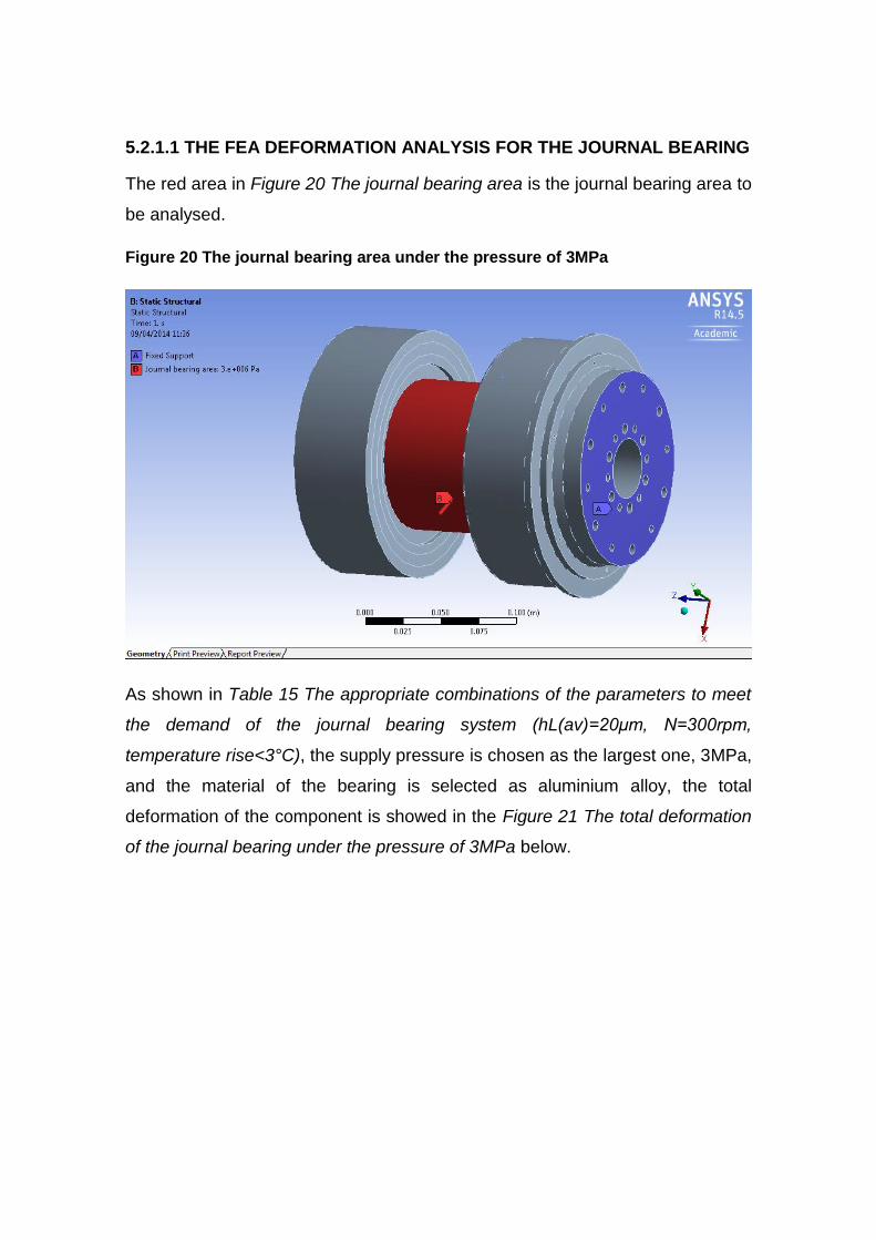
5.2.1.1 THE FEA DEFORMATION ANALYSIS FOR THE JOURNAL BEARING
The red area in Figure 20 The journal bearing area is the journal bearing area to
be analysed.
Figure 20 The journal bearing area under the pressure of 3MPa
As shown in Table 15 The appropriate combinations of the parameters to meet
the demand of the journal bearing system (hL(av)=20μm, N=300rpm,
temperature rise<3°C), the supply pressure is chosen as the largest one, 3MPa,
and the material of the bearing is selected as aluminium alloy, the total
deformation of the component is showed in the Figure 21 The total deformation
of the journal bearing under the pressure of 3MPa below.

Figure 21 The total deformation of the journal bearing under the pressure of
3MPa
From the figure above, the maximum deformation, i.e. the red part, happens in
the middle of the bearing thrust plate, whose value is about 2.973μm. Since it is
an inward deformation, it will not cause extra wear or friction to the inner surface
of the pocket house. In the area of green or yellow colour, the deformation is
even smaller, about 2μm and also inward direction.
So from the FEA modelling analysis, the aluminium bearing shaft is capable of
the supply pressure of 3MPa and its deformation will not influence the normal
working of the hydrostatic bearing system. But the deformation will slightly
increase the flow rate at some level due to the small increase of the radial
clearance.

5.2.1.2 THE FEA DEFORMATION ANALYSIS FOR THE THRUST BEARING
The middle circular ring of the red area in the following figure is the thrust
bearing pocket area, and the inner and outer rings of the red area is the land
area of the thrust bearing plate. The pocket area and the land area will be
applied different pressure to analyse the deformation condition due to the
decrease of the pocket pressure.
Figure 22 The thrust bearing area under the pocket area pressure of 2MPa and
the average land area pressure of 1MPa
As recommended in the Table 20 The appropriate combinations of the
parameters to meet the demand of the thrust bearing system (hd=20μm,
N=300rpm, temperature rise<3ºC), the supply pressure in the pocket area is
2MPa, the average pressure in the land area is 1MPa, and the material of the
bearing is selected as aluminium alloy, the total deformation of the component
is shown in the Figure 23 The total deformation of the thrust bearing under the
pocket area pressure of 2MPa and the average land area pressure of 1MPa
below.
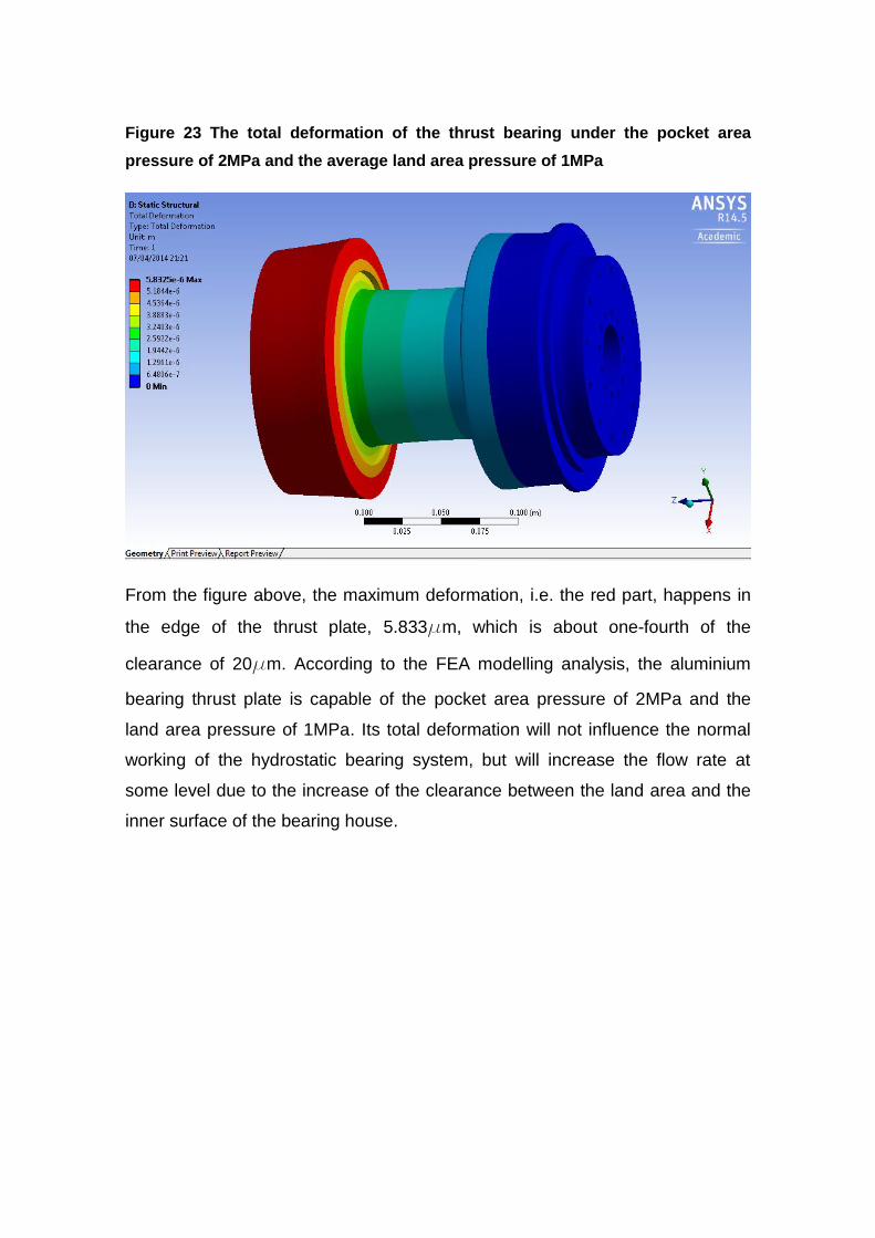
Figure 23 The total deformation of the thrust bearing under the pocket area
pressure of 2MPa and the average land area pressure of 1MPa
From the figure above, the maximum deformation, i.e. the red part, happens in
the edge of the thrust plate, 5.833μm, which is about one-fourth of the
clearance of 20μm. According to the FEA modelling analysis, the aluminium
bearing thrust plate is capable of the pocket area pressure of 2MPa and the
land area pressure of 1MPa. Its total deformation will not influence the normal
working of the hydrostatic bearing system, but will increase the flow rate at
some level due to the increase of the clearance between the land area and the
inner surface of the bearing house.

5.2.1.3 THE FEA DEFORMATION ANALYSIS FOR BOTH THE THRUST
BEARINGS AND THE JOURNAL BEARING
Combining two pressure conditions together, 3MPa on the journal bearing area,
2MPa on the thrust plate pocket area, and 1MPa on the thrust plate land area,
the pressure condition is shown in Figure 24 The overall pressure condition for
the combination of journal bearing pressure 3MPa, thrust plate pocket area
pressure 2MPa, and the thrust plate land area pressure 1MPa.
Figure 24 The overall pressure condition for the combination of journal bearing
pressure 3MPa, thrust plate pocket area pressure 2MPa, and the thrust plate land
area pressure 1MPa
The total deformation analysis solution of the bearing system is showed in the
following figure.

Figure 25 The total deformation for the combination of journal bearing pressure
3MPa, thrust plate pocket area pressure 2MPa, and the thrust plate land area
pressure 1MPa
The maximum deformation happens in the edge of the thrust plate, which is
about 6.853µm.
Under 20µm and less than 3ºC, the 6.853µm is about 34.3% of the clearance.
As a result, whether the pressure and the oil viscosity are appropriate or not
needs to be analysed in further experimental works.
For the clearance of 30µm and the temperature rise smaller than 3ºC, the
6.853µm is about 22.8% of the clearance. Similarly, whether the combination is
feasible or not needs to be analysed in further experimental works.
Considering the 3 times factor of safety, the pressure on the journal area is
1.5MPa, the pressure on the thrust pocket area is 0.3MPa and the pressure on
the thrust land area is 0.15MPa, the overall pressure condition is shown in
Figure 26 The overall pressure condition for the combination of journal bearing
pressure 1.5MPa, thrust plate pocket area pressure 0.3MPa, and the thrust
plate land area pressure 0.15MPa.

Figure 26 The overall pressure condition for the combination of journal bearing
pressure 1.5MPa, thrust plate pocket area pressure 0.3MPa, and the thrust plate
land area pressure 0.15MPa
The total deformation analysis solution of the bearing system is shown in Figure
27 The total deformation for the combination of journal bearing pressure
1.5MPa, thrust plate pocket area pressure 0.3MPa, and the thrust plate land
area pressure 0.15MPa. Due to the neutralization of the displacement
generated separately by the pressure on journal bearing and the thrust bearing,
the maximum deformation, about 1.829µm, does not happen on the edge of the
thrust plate but in the middle of it, which will cause less effect on the normal
working process and will probably not cause the extra friction or contact inside
the bearing house. So, the combination of relatively larger journal bearing
pressure and smaller thrust bearing pressure will tend to neutralize the
deformation conditions and partly strengthen the performance of the hydrostatic
bearing system.

Figure 27 The total deformation for the combination of journal bearing pressure
1.5MPa, thrust plate pocket area pressure 0.3MPa, and the thrust plate land area
pressure 0.15MPa

5.2.1.4 THE FEA ANALYSIS RESULTS OF THE TABLES OF SOME SETS
OF THE COMBINATIONS OF SUPPLY PRESSURE AND OIL
VISCOSITY
After the optimization works done in the previous sections, the viscosity of oil is
selected as two values, 5cSt and 10cSt. For each of these two viscosities, set
the journal supply pressure as 1.5MPa, 3MPa and 5MPa, the thrust bearing
pocket pressure as 0.3MPa, 0.5MPa and 1MPa.
Set da, db, and dc as three observation points to analyse the deformation
condition of the hydrostatic bearing, which is showed in the following figure. da
is the radial clearance of the journal bearing, db is the minimum deformation
place of the thrust plate and dc is the maximum deformation place of the thrust
plate.
Figure 28 Three deformation analysis points

According to Equation 8 and Equation 17, the value of the flow rate is
proportional to the cube of the bearing clearance. So after the deformation, the
actual clearances both in journal bearing and thrust bearing will be larger than
the nominal clearance, which means the actual flow rate will be larger than the
nominal flow rate as well as the temperature rise is smaller than the nominal
value. So the values of the nominal clearance, actual clearance, nominal flow
rate, actual flow rate, nominal temperature rise, and actual temperature rise for
both journal bearing and thrust bearing are also showed in the FEA results
tables.
For the Set 1 analysis (hc=20µm, η=5cSt Pjournal=1.5MPa, Pthrust pocket=0.3MPa,
Pthrust land=0.15MPa, N=300rpm), as showed in the follow figures, the
deformation of da=1.307µm, db=1.437µm, and dc=1.307µm.
Figure 29 The pressure condition for Set 1 analysis
The flow rate is show in the following table.
Table 23 The FEA results table for set 1 analysis
η=5cSt,N=300rpm
Pjournal=1.5MPa,Pthrust=0.3MPa
Clearance (µm)
Flow rate (L/min)
Temperature rise (ºC)

Journal bearing
Nominal value 20 0.321 1.911
Actual value 21.30737 0.388 1.670
Thrust bearing
Nominal value 20 0.140 4.451
Actual value 21.37238 0.171 3.459
Figure 30 The deformation solution for Set 1 analysis
From the Table 23 The FEA results table for set 1 analysis, it is concluded that
the actual flow rate is larger and the actual temperature rise is smaller than the
nominal ones due to the deformation of the bearing component. So at this level,
the appropriate deformation is somehow beneficial to the hydrostatic bearing
systems.
The following table shows all sets of the FEA analysis results. The clearances
are 20µm and 30µm, the viscosities are 5cSt and 10cSt, the rotational speed is
300rpm, and the supply pressure combinations are Pjournal=1.5MPa & Pthrust
pocket=0.3MPa, Pjournal=3MPa & Pthrust pocket=1MPa, and Pjournal=5MPa & Pthrust
pocket=2MPa.
37 Actual journal bearing clearance=nominal journal bearing clearance + da
38 Actual thrust bearing clearance=nominal thrust bearing clearance + 0.5*(db + dc)

Table 24 The FEA analysis results
Rotational speed N=300rpm
Bearing clearance (µm)
20 30
Viscosity (cSt) 5 10 5 10
Journal bearing
Nominal value
Pressure (MPa) 1.5 3 5 1.5 3 5 1.5 3 5 1.5 3 5
Clearance (µm) 20 20 20 20 20 20 30 30 30 30 30 30
Flow rate (L/min) 0.321 0.641 1.069 0.160 0.321 0.534 1.082 2.164 3.607 0.541 1.082 1.803
Temperature rise (ºC)
1.911 2.206 3.101 5.146 3.823 4.072 1.045 1.773 2.841 1.682 2.091 3.032
Actual value
da (µm) 1.307 2.952 5.958 1.307 2.952 5.958 1.307 2.952 5.958 1.307 2.952 5.958
Clearance (µm) 21.307 22.952 25.958 21.307 22.952 25.958 31.307 32.952 35.958 31.307 32.952 35.958
Flow rate (L/min) 0.388 0.969 2.337 0.194 0.485 1.168 1.230 2.868 6.211 0.615 1.434 3.105
Temperature rise (ºC)
1.670 1.977 2.891 4.179 2.908 3.233 1.012 1.739 2.809 1.548 1.958 2.901
Thrust bearing
Nominal value
Pressure (MPa) 0.3 1 2 0.3 1 2 0.3 1 2 0.3 1 2
Clearance (µm) 20 20 20 20 20 20 30 30 30 30 30 30
Flow rate (L/min) 0.140 0.467 0.934 0.070 0.233 0.467 0.473 1.575 3.151 0.236 0.788 1.575
Temperature rise (ºC)
4.451 1.841 1.754 17.305 5.697 3.682 1.024 0.813 1.240 3.597 1.585 1.626
Actual value
db (µm) 1.437 3.543 6.499 1.437 3.543 6.499 1.437 3.543 6.499 1.437 3.543 6.499
dc (µm) 1.307 3.838 7.041 1.307 3.838 7.041 1.307 3.838 7.041 1.307 3.838 7.041
Clearance (µm) 21.372 23.691 26.770 21.372 23.691 26.770 31.372 33.691 36.770 31.372 33.691 36.770
Flow rate (L/min) 0.171 0.776 2.239 0.085 0.388 1.119 0.540 2.231 5.801 0.270 1.116 2.901
Temperature rise (ºC)
3.459 1.212 1.313 13.334 3.180 1.919 0.885 0.718 1.169 3.041 1.206 1.341

From the table above, the deformation of the bearing components due to the
large pressure exerted on their surfaces will affect the actual performance of the
hydrostatic bearing systems. The actual flow rate is larger than the nominal flow
rate and the actual temperature rise is smaller than the nominal one due to the
increasing flow rate of the oil.
However the increasing bearing clearance has a limited influence on the
temperature rise of the bearing systems. When the original bearing clearance is
large, the influence on the temperature rise by increasing the bearing clearance
is relatively small compared with the situation that the original bearing clearance
is relatively small as illustrated in the following table:
Table 25 The comparison between the influences on the temperature rise by
increasing bearing clearance at different initial bearing clearance
Journal bearing
Viscosity (cSt) 10 10
Bearing pressure (MPa) 5 5
Nominal bearing clearance (µm) 20 30
Actual bearing clearance (µm) 25.958 35.958
Nominal flow rate (L/min) 0.534 1.803
Actual flow rate (L/min) 1.168 3.105
Nominal temperature rise (ºC) 4.072 3.032
Actual temperature rise (ºC) 3.233 2.901
Thrust bearing
Viscosity (cSt) 10 10
Bearing pressure (MPa) 2 2
Nominal bearing clearance (µm) 20 30
Actual bearing clearance (µm) 26.770 36.770
Nominal flow rate (L/min) 0.467 1.575
Actual flow rate (L/min) 1.119 2.901
Nominal temperature rise (ºC) 3.682 1.626
Actual temperature rise (ºC) 1.919 1.341
From the table above, the actual temperature rise drops more at the initial
bearing clearance of 20µm than that of 30 µm.

For the journal bearing, the actual temperature rise drops about 20.6% at the
initial clearance of 20µm and only 4.3% at the initial clearance of 30µm.
For the thrust bearing, the actual temperature rise drops about 47.9% at the
initial clearance of 20µm and only 17.5% at the initial clearance of 30µm.
By the definition of the equation of the temperature rise, Equation 11 and
Equation 20, the two main source of the temperature rise is pumping power and
the frictional power.
Under the larger initial clearance condition, the larger initial flow rate due to the
larger initial bearing clearance almost brings all the frictional power generated
by the frictional force due to the friction between the bearing surfaces and the
oil even before the deformation happens, so the main energy source of the
temperature rise is just the pumping power. The larger the pumping power is,
the higher the supply pressure will be, and the higher the temperature rise will
be regardless of the subsequent increasing bearing clearance due to the
deformation of the bearing components.
For the smaller initial clearance cases, the frictional power is partially carried
away by the relatively small flow rate, so the rest of the frictional power as well
as the pumping power are both the main sources of the temperature rise. When
the bearing clearance increases, the flow rate also increases and then carries
away more frictional power. So in this condition, the deformation of the bearing
part is beneficial to lower the temperature rise without at the cost of losing the
accuracy by increasing the initial bearing clearance.
As a conclusion, the influence to reduce the temperature rise by increasing the
bearing clearance is limited. Within a specific range of initial bearing clearance,
the deformation of the bearing part at the supply pressure has a relatively large
influence on reducing the temperature rise of the bearing system. But when the
initial bearing clearance exceeds a specific value, which is about 30µm in this
case, the influence on reducing the temperature rise under the deformation
condition is greatly diminished for there is no more extra frictional power to be
carried away at an unchanged rotational speed.

For the following table, when the initial clearance is 20 µm, the viscosity of oil is
10cSt, the journal supply pressure is 1.5MPa, and the thrust bearing supply
pressure is 0.3MPa, the temperature rise performance is not very satisfied,
being 4.179ºC and 13.334ºC respectively, which does not meet the requirement
of the temperature rise being less than 3 ºC. So in a real experimental, this
combination of the input parameters shall be avoided.
Table 26 The flow rate and temperature rise conditions at low supply pressure
and high oil viscosity
Journal bearing
Viscosity (cSt) 10
Bearing pressure (MPa) 1.5
Nominal bearing clearance (µm) 20
Actual bearing clearance (µm) 21.307
Nominal flow rate (L/min) 0.160
Actual flow rate (L/min) 0.194
Nominal temperature rise (ºC) 5.146
Actual temperature rise (ºC) 4.179
Thrust bearing
Viscosity (cSt) 10
Bearing pressure (MPa) 0.3
Nominal bearing clearance (µm) 20
Actual bearing clearance (µm) 21.372
Nominal flow rate (L/min) 0.070
Actual flow rate (L/min) 0.085
Nominal temperature rise (ºC) 17.305
Actual temperature rise (ºC) 13.334
From the Table 24 The FEA analysis results, most of the actual temperature
rise is less than 3ºC. The experimental input parameters can be chosen not
only according to the ANSYS analysis results but also to the availability of the
actual experimental equipment of different parameters, because for most of the
combinations in the result analysis, the temperature rise lies within the
requirement range less than 3ºC.

6 EXPERIMENTAL PROCEDURES
6.1 THE EXPERIMENTAL INPUT PARAMETERS SELECTIONS
BASED ON THE THEORETICAL CALCULATIONS AND
FINITE ELEMENT ANALYSIS
After the theoretical calculations and FEA work, the experimental input
parameters could be decided preliminarily.
6.1.1 THE OIL TYPE
From the Table 24 The FEA analysis results, except the extreme condition
illustrated in the Table 26 The flow rate and temperature rise conditions at low
supply pressure and high oil viscosity, whose temperature rise greatly exceeds
3ºC, most of the results are suitable for the normal operational conditions of the
system.
The lower viscosity is recommended to be used in the hydrostatic bearing
system such as 10cSt or 15cSt.
6.1.2 THE SUPPLY PRESSURE
For the lower pressure supply, journal bearing pressure 3MPa and thrust
bearing pressure 1.5MPa, the temperature rise is always larger than 3ºC, so
this combination can be removed.
For the journal bearing pressure 2MPa and thrust bearing pressure 1MPa or the
journal bearing pressure 5MPa and thrust bearing pressure 2MPa, the
temperature rise is appropriate. The higher supply pressure means the higher
energy consumption and pumping power generation. And the temperature rise
of higher supply pressure is higher than that of lower supply pressure under
some conditions. So the 5MPa and 2MPa combination can also be ignored.
As a result, the combination of journal bearing pocket pressure 3MPa and thrust
bearing pocket pressure 1MPa is chosen as the experimental supply pressure.
Considering the resistance ratio of journal resistor is 1 and thrust resistor is 5,
the supply can be set at about 6MPa (60Bar) to get the pocket pressure of
3MPa and 1MPa respectively.

6.1.3 THE BEARING CLEARANCE
The bearing clearance is closely related to the radial stiffness and the
manufacturing cost. The larger the bearing clearance is, the lower the radial
stiffness and the manufacturing cost will be. Apparently, the lower cost is good
for the project, but the low stiffness is not beneficial to the system.
For the journal bearing, the relationship within radial clearance, radial stiffness
and temperature rise is showed in the following table.
Table 27 The relationship between the radial clearance, radial stiffness and
temperature rise of the journal bearing (p=3MPa, ŋ=10.00cSt, N=300rpm)
Radial clearance(µm) Radial stiffness (108N/m) Temperature rise (°C)
10 12.626 36.308
20 6.313 3.823
25 5.051 2.548
30 4.209 2.091
40 3.157 1.800
50 2.525 1.721
60 2.104 1.693
For the journal loading condition of 1500N, the displacement of the bearing
shaft under the radial stiffness of 4.209*108N/m is 3.563µm, which is an
acceptable value compared with original radial clearance of 30µm. And the
temperature rise for 30µm clearance is 2.091ºC, which is also an acceptable
value. The suitable radial clearance for journal bearing is 30µm.
For the thrust bearing, the relationship within radial clearance, radial stiffness
and temperature rise is showed in the following table.
Table 28 The relationship between the thrust bearing clearance, stiffness and
temperature rise of the thrust bearing (p=1MPa, ŋ=10.00cSt, N=300rpm)
Clearance (µm) Stiffness (108N/m) Temperature rise (°C)
10 8.903 87.725
20 4.452 5.697

25 3.561 2.676
30 2.968 1.585
40 2.226 0.885
50 1.781 0.692
60 1.484 0.622
For the thrust loading condition of 500N, the displacement of the thrust plate
under the stiffness of 2.968*108N/m is 1.685µm, which is an acceptable value
compared with the original clearance of 30µm. And the temperature rise for
30µm is 1.585ºC, which is also an acceptable value. The suitable clearance for
thrust bearing is also 30µm.
There is still another choice that the bearing clearance could be chosen as the
mid value of 20µm and 30µm, which is 25µm. The theoretical calculation table
is showed in the following table.
Table 29 The theoretical calculation table when the clearance is 25µm
Rotational speed
N=300rpm
Bearing clearance (µm)
25
Viscosity (cSt) 5 10
Journal
bearing
Nominal value
Pressure (MPa) 1.5 3 5 1.5 3 5
Clearance (µm) 25 25 25 25 25 25
Flow rate (L/min) 0.626 1.252 2.087 0.313 0.730 1.044
Temperature rise (ºC) 1.274 1.887 2.910 2.596 2.385 3.307
Actual value
da (µm) 1.307 2.952 5.958 1.307 2.952 5.958
Clearance (µm) 26.307 27.952 30.958 26.307 27.952 30.958
Flow rate (L/min) 0.730 1.750 3.963 0.365 0.875 1.982
Temperature rise (ºC) 1.193 1.807 2.834 2.270 2.230 3.002
Thrust
bearing
Nominal value
Pressure (MPa) 0.3 1 2 0.3 1 2
Clearance (µm) 25 25 25 25 25 25
Flow rate (L/min) 0.274 0.912 1.823 0.137 0.456 0.912
Temperature rise (ºC) 1.933 1.086 1.376 7.233 2.676 2.171
Actual value
db (µm) 1.437 3.543 6.499 1.437 3.543 6.499
dc (µm) 1.307 3.838 7.041 1.307 3.838 7.041

Clearance (µm) 26.372 28.691 31.770 26.372 28.691 31.770
Flow rate (L/min) 0.321 1.378 3.742 0.161 0.689 1.871
Temperature rise (ºC) 1.596 0.863 1.214 5.884 1.784 1.521
From the data above, although the clearance is selected as the mid value of
20µm and 30µm, the most suitable combination is still 10cSt, journal bearing
pressure 3MPa and thrust bearing pressure 1MPa. And according to the Table
27 The relationship between the radial clearance, radial stiffness and
temperature rise of the journal bearing (p=3MPa, ŋ=10.00cSt, N=300rpm) and
Table 28 The relationship between the thrust bearing clearance, stiffness and
temperature rise of the thrust bearing (p=1MPa, ŋ=10.00cSt, N=300rpm), the
clearance of 25µm can always meet all the requirement of journal radial
stiffness, thrust axial stiffness and the temperature rise. So if the experimental
budget is sufficient, the hydrostatic bearing systems of the bearing clearance of
25µm are also strongly recommended to be manufactured to analyse and test
the systems in the further experimental works.
6.1.4 THE EXPERIMENTAL INPUT PARAMETERS COMBINATION
As a general conclusion based on the initial calculation, ANSYS modelling
simulation and the initial data analysis, one of the theoretically suitable input
parameters is listed in the following table:
Table 30 One of the suitable experimental input parameters combinations
Experimental input parameters selections
Oil viscosity 10 cSt
Journal bearing supply pressure 3 MPa
Thrust bearing supply pressure 1 MPa
Bearing clearance 25 or 30 µm
Rotational speed 300 rpm
If the budget is sufficient, the hydrostatic bearing systems of both 25µm
clearance and 30µm clearance or the oil viscosity of both 10cSt and 15cSt shall
be tested to prove their working performance.

6.1.5 THE POWER CONSUMPTION CONDITION UNDER THE
RECOMMENDED COMBINATION
Under 25µm, 300rpm, 10cSt, journal bearing pressure 3MPa and thrust bearing
pressure 1MPa, the power consumption condition is showed in the following
table.
Table 31 The power consumption condition under the recommended
combination (h=25µm, N=300rpm, ŋ=10cSt, Pjournal=3MPa, Pthrust=1MPa)
Pumping power Frictional power Total power
Journal bearing 31.31W 16.56W 47.87W
Thrust bearing 15.19W 28.99W 44.18W
Under 30µm, 300rpm, 10cSt, journal bearing pressure 3MPa and thrust bearing
pressure 1MPa, the power consumption condition is showed in the following
table.
Table 32 The power consumption condition under the recommended
combination (h=30µm, N=300rpm, ŋ=10cSt, Pjournal=3MPa, Pthrust=1MPa)
Pumping power Frictional power Total power
Journal bearing 54.10W 13.77W 67.87W
Thrust bearing 26.26W 24.32W 50.58W
If the deformation is taken into consideration, after the ANSYS modelling, the
new tables are showed below.
Table 33 The power consumption condition under the recommended
combination after ANSYS modelling (h=25µm, h’journal=27.952µm,
h’thrust=28.691µm, N=300rpm, ŋ=10cSt, Pjournal=3MPa, Pthrust=1MPa)
Pumping power Frictional power Total power
Journal bearing 43.76W 14.79W 58.55W
Thrust bearing 22.97W 25.39W 48.36W

Table 34 The power consumption condition under the recommended
combination after ANSYS modelling (h=30µm, h’journal=32.952µm,
h’thrust=33.691µm, N=300rpm, ŋ=10cSt, Pjournal=3MPa, Pthrust=1MPa)
Pumping power Frictional power Total power
Journal bearing 71.70W 12.52W 84.22W
Thrust bearing 37.19W 21.76W 58.95W
From the tables above, the results can be listed as the following points:
The total power consumption of journal bearing is larger than that of the
thrust bearing;
The pumping power increases after the deformation due to the extra
energy to maintain the same supply pressure as well as the extra flow
rate;
The frictional power decreases after the deformation due to the
increased clearance;
The total power consumption of both initial clearance and both bearing
types increases after the deformation.
6.1.6 THE REYNOLDS NUMBER CONDITION UNDER THE
RECOMMENDED INPUT COMBINATION
The equations for frictional power, Equation 9, Equation 10, Equation 18 and
Equation 19, are all based on the assumption that the fluid flow in the pocket is
laminar flow39 . However, the flow will become turbulent above a particular
speed of the journal or the thrust bearings. The turbulence in the pocket will
cause the “fluid friction” over the area of the pocket rise more rapidly with speed
(Stansfield, 1970).
The value of Reynolds Number (Re) indicates whether the turbulence is likely to
occur. The equation for Re is listed below:
39 Laminar flow (or streamline flow) occurs when a fluid flows in parallel layers, with no disruption between
the layers.

Reynolds Number
Equation 30
Under 25µm, 300rpm, 10cSt, journal bearing pressure 3MPa and thrust bearing
pressure 1MPa, the Reynolds numbers are listed below:
Table 35 The Reynolds number condition under the recommended combination
before and after ANSYS modelling (h=25µm, h’journal=27.952µm, h’thrust=28.691µm,
N=300rpm, ŋ=10cSt, Pjournal=3MPa, Pthrust=1MPa)
Journal bearing Thrust bearing
Re (before deformation) 7.83 11.38
Re (after deformation) 8.76 13.06
Under 30µm, 300rpm, 10cSt, journal bearing pressure 3MPa and thrust bearing
pressure 1MPa, the Reynolds numbers are listed below:
Table 36 The Reynolds numbers under the recommended combination before
and after ANSYS modelling (h=30µm, h’journal=32.952µm, h’thrust=33.691µm,
N=300rpm, ŋ=10cSt, Pjournal=3MPa, Pthrust=1MPa)
Journal bearing Thrust bearing
Re (before deformation) 9.40 13.66
Re (after deformation) 10.33 15.34
The Reynolds numbers under all the conditions are less than 2000, which is the
critical point between laminar flow and turbulence, so the fluid within the
hydrostatic bearings is always regarded as the laminar, just verifying the
assumptions before.
Another conclusion is that the Reynolds numbers are slightly larger after the
deformation. At lower rotational speed, the clearance change is not obvious
enough to affect the Reynolds number. But at high rotational speed and low
viscosity, the deformation is likely to increase the Reynolds number a lot and
will influence the normal performance of the hydrostatic bearing systems.

6.2 THE MEASUREMENT AND MACHINING PROCESS OF THE
HYDROSTATIC BEARINGS
6.2.1 THE MEASUREMENT OF THE BEARING CONPONENTS
To achieve the ideal bearing gap of about 25-30µm, some ultra-precision
measurement equipment is necessary to define the dimensions of the bearing
parts.
Each component, including bearing shafts, thrust plates and bearing housing,
shall be measured at least three times:
The 1st time: after the aluminium parts being machined by the diamond turning
and before the parts being coated, to get the original dimension of the
hydrostatic bearing system;
The 2nd time: after the bearing parts being coated and before the second
diamond turning process, probably the most important measurement process
not only to know the thickness of the coating and but also to decide the amount
of the coating to be removed to achieve the target bearing clearance;
The 3rd time: after the second diamond turning, to check the final dimension of
the bearing system to see whether it meets the design requirement.
The figures below are the components after being coated and before the
second diamond turning process:

Figure 31 The bearing shaft after being coated and before the second diamond
turning process
Figure 32 The thrust plate after being coated and before the second diamond
turning process

Figure 33 The bearing house after being coated and before the second diamond
turning process
The following tools are some hand measuring tools in the laboratory:
The TESA IMICRO with analogue indication 90-10040 is used to measure the
inner diameter of the bearing house. Its measuring span is 90-100mm, its scale
interval is 0.002mm and its maximum permissible error is 0.005µm.
Figure 34 TESA IMICRO with analogue indication 90-100
The Moore & Wright traditional depth gauge micrometer41 is used to measure
the length of the journal and the depth of the bearing house. Its measuring span
40 Data from: http://www.tesagroup.co.uk/en-us/products/tesa-imicro-with-analogue-indication-metric-
p152.htm?redirect=1&c=gb#.U3d6YqNwbcs

is 0-75mm, its scale interval is 0.01mm and its maximum permissible error is
0.01mm.
Figure 35 The Moore & Wright depth gauge micrometer
The Moore & Wright outside micrometer42 is used to measure the thickness of
the thrust bearing. Its measuring span is 50-75mm, its scale interval is 0.002mm
and its maximum permissible error is 0.01mm.
Figure 36 The Moore & Wright outside micrometer
The Mitutoyo caliper digital absolute IP6743 is used to measure both the inside
and outside distances between two parallel surfaces. Its measuring span is 0-
150mm, its scale interval is 0.01mm and its maximum permissible error is
0.01mm.
41 Data from: http://www.moore-and-wright.com/products/show/13904?lang=English
42 Data from: http://www.moore-and-wright.com/products/show/4682?lang=English
43 Data from: http://uk.farnell.com/mitutoyo/500-706-11/caliper-digital-absolute-ip67-150mm/dp/1698141

Figure 37 The Mitutoyo caliper digital absolute IP67
The minimum error of all these hand measuring tools is 5µm, which is relatively
a large number compared with the target clearance of 25-30µm. So the
machining process based on these hand measuring tools is not reliable and will
not actually reflect the results from the previous theoretical.
So the ultra-precision coordinate measuring machine, Leitz PMM-F 100044, is
introduced to measure the dimension of the bearing house and shaft.
Figure 38 Leitz PMM-F 1000 CMM
44 Data from:
http://www.hexagonmetrology.com.cn/uploadfiles/File/%E6%A0%B7%E6%9C%AC/Product_Overview_Err
orCharts.pdf

Its measuring span is 3000*2000*1000mm, its volumetric length measuring
error E is defined in the following equation:
Volumetric length measuring error E45 Equation 31
For the bearing components less than 300mm, the error of the CMM machine
on this specific component is less than 2.45µm, which is smaller than the value
of about 10% of the target clearance.
So the dimensions measured by the PMM-F 1000 can be used to machine the
bearing components to get the required bearing clearance. The measuring
process is showed in the following figure:
Figure 39 The bearing house is being measured by the Leitz CMM
45 Data from:
http://www.hexagonmetrology.com.cn/uploadfiles/File/%E6%A0%B7%E6%9C%AC/Product_Overview_Err
orCharts.pdf

6.2.2 THE DIMENSIONS OF THE EXPERIMENTAL COMPONENTS
After the measurement by CMM, the dimensions of the components are listed
below:
Table 37 The dimensions of the experimental components
Bearing housing
Small inside diameter 99.805 Mm
Large inside diameter 163.765 Mm
Working thickness over lands 71.995 Mm
Spindle bearing
Small diameter 99.748 Mm
Large diameter 163.718 Mm
Working thickness over lands 72.053 Mm
Thrust bearing
Outside diameter 163.775 Mm
Thickness 53.700 Mm
Rear housing
Large diameter 164.035 Mm
From the table above, the crucial dimensions showed in the following figure can
be calculated.

Figure 40 The important dimensions of the experimental components
The spindle journal bearing radial clearance:
The spindle bearing and thrust bearing gap:
The spindle bearing radial clearance:
The thrust bearing radial clearance:

The spindle journal bearing radial clearance and the spindle bearing gap are the
hydrostatic bearing parameters, which are both very important to the
experiment. And their values are machined at about 30µm.
The spindle bearing radial clearance is 23.5µm, which is relatively small
compared with the bearing clearance of about 30µm. However, it still conforms
to the blueprint drawings. The other thrust bearing radial clearance, whose
value is 130µm, is large enough to lay in the safety areas to prevent any extra
wear circumstances.
6.2.3 THE MACHINING PROCESS OF THE BEARING COMPONENTS
The EPSRC Centre for innovative manufacturing in ultra-precision at Cranfield
University uses the CUPE Nanocentre to machine the hydrostatic bearing
components. It uses diamond tool to machine the aluminium alloy materials.
And its error is about 100nm, which greatly meets the demand of the design of
the hydrostatic bearing system of 25-30µm.

Figure 41 The CUPE nanocentre in the EPSRC Centre at Cranfield University
The following picture is the baring house which is machined after the coating
process.
Figure 42 The re-machined bearing house after the coating process

6.3 THE PARAMETERS MEASUREMENT AND THE TEST
EQUIPMENT
The aim of the experimental works is to measure some important parameters of
the system to find out whether the new aluminium hydrostatic bearing systems
can be qualified and economical substitutions to the expensive steel ones.
6.3.1 THE INPUT PARAMETERS AND THE EQUIPMENT
6.3.1.1 THE SUPPLY PRESSURE
The supply pressure, one of the most important input parameters, could be set
by the hydraulic supply system by adjusting the rotational speed of the pump
motor. The higher the speed is, the higher the supply pressure will be. For any
group of experiment result, the supply pressure is always one of the most
fundamental precondition parameters. The supply pressure is relevant to most
of the parameters of the hydrostatic bearing system, such as the ultimate load
capacity, the flow rate, the power consumption, the bearing deformation (the x
displacement), the stiffness, and even the temperature rise.
Figure 43 The experimental inverter

The inverter46 is HITACHI SJ100 Series Inverter47, which is showed in the figure
above. Its main features are listed below and its specifications are showed in
the 8Appendix C THE SPECIFICATIONS FOR SJ100 INVERTER.
Figure 44 HITACHI SJ100 Series Inverter
Figure 45 The ABB M2AA 090 L-4 motor
46 The term inverter and variable-frequency drive are related and somewhat interchangeable. An electronic
motor drive for an AC motor can control the motor’s speed by varying the frequency of the power sent to
the motor. An inverter, in general, is a device that converts DC power to AC power. The drive first converts
incoming AC power to DC through a rectifier bridge, creating an internal DC bus voltage. Then the inverter
circuit converts the DC back to AC again to power the motor. The special inverter can vary its output
Frequency and voltage according to the desired motor speed.
47 Data from: https://www.automationdirect.com/static/manuals/sj100/sj100.pdf

The motor is ABB M2AA 090 L-448 series motor, which is showed in the Figure
45 The ABB M2AA 090 L-4 motor above. It is a general-purpose aluminium
motor. The three phase motors are ideal for a wide variety of applications
including pumps, fans and process machinery drives. Motors in frame sizes 63-
100 may be connected in either STAR (Y) for supply voltages of 380-420//440-
480V 50/60Hz or DELTA for 220-240//250-280 50/60Hz. Motors in frame sizes
112-132 are suitable DELTA connected 380-420//440-480V 50/60Hz and are
also suitable for STAR/DELTA starting. Its specifications are showed in
8Appendix D THE SPECIFICATIONS FOR ABB M2AA 090 L-4 MOTOR and
the following are its main characteristics:
Top mounted terminal box with metric/Pg type knockouts;
Energy efficient low noise design;
Corrosion resistant, low copper aluminium alloy;
Suitable for DOL starting or inverter drive use.
The supply pressure could be measured by 63mm pressure gauges49, which is
illustrated in the following picture.
Figure 46 The pressure gauge for pressure from 10MPa to 69MPa
48 Data from: http://il.rsdelivers.com/product/abb/m2aa-90l/3phase-2p-flange-induction-motor-
22kw/3290874.aspx
49 Data from: http://www.hydrotechnik.co.uk/catalog/measurement-equipment-sensors/gauges-switches-
displays/analogue-pressure-gauges/63mm-bottom-

6.3.1.2 THE POCKET PRESSURE
The pocket pressure of each bearing pocket can be measured by the pressure
gauges as the figure below. There are seven pockets on the bearing system:
five journal bearing pockets and two thrust baring pockets. Each of these
pockets has a hole to the surface of the bearing housing. These holes can be
inserted a pressure gauge to monitor the pocket pressure.
Figure 47 Pressure gauge to measure the pocket pressure
Figure 48 Hole on the bearing housing to insert the pressure gauge

6.3.1.3 THE FLUID VISCOSITY
For any oil lubrication system, oil viscosity50 is always considered as one of the
most important parameters. The fluid viscosity, also one of the most important
input parameters relevant to the flow rate and the temperature change during
the operational process, could be decided by the pre-selection of the oil type.
However the viscosity of the oil is not constant, it will decrease as the
temperature increases. So in this report, a basic assumption is made, as
showed in the Assumption 2 that the viscosity change due to the temperature
change during the operational process of the hydrostatic bearing system is
ignored. The only value considered is the viscosity of oils of the various types.
The viscosity can usually be measured by means of the viscosity comparator
a.k.a. viscostick, the viscotube, or the viscometer51. The dial reading viscometer
is showed in the following figure.
Figure 49 Dial Reading Viscometer
50 Viscosity can be defined as measurement of fluid internal resistance to flow at a specified temperature.
There are two ways to measure a fluid’s viscosity, namely Dynamic (Absolute) Viscosity and Kinematic
Viscosity. Both dynamic and kinematic viscosity are interchangeable by using the formula below:
Dynamic Viscosity (cP) = Kinematic Viscosity (cSt) x Fluid Density (g/cm3)
51 Data from: http://www.kittiwake.com/sites/default/files/2%20-%20Viscosity%20Dec12_0.pdf

For the ultra-precision hydrostatic bearing system, whose components surfaces
are separated by an oil film of about 20 microns or less and the supply pressure
is relatively high, the viscosity monitoring is very important to maintain the
viscosity of the oil staying within the suitable range of the correct oil viscosity
values. Any sudden significant change of the oil viscosity, either reduction or
increment, may affect the stability and the effectiveness of the lubrication film,
which is showed in the following table:
Table 38 Effect of the change of the viscosity of the oil52
Reduction in Viscosity Increase in Viscosity
Loss of oil film resulting in excessive wear
Increased mechanical friction causing excessive energy consumption and heat generation
Increased sensitivity to particle contamination due to reduced oil film thickness
Oil film failure at high temperatures, high loads during start-ups or coast-downs
Excessive heat generation resulting in oil oxidation, sludge and varnish build-up
Gaseous cavitation due to inadequate oil flow to pumps and bearings
Lubrication starvation due to inadequate oil flow
Oil whip in journal bearings
Excess energy consumption to overcome fluid friction
Poor air detrainment or demulsibility
Poor cold start pumpability.
The effects above will finally result in the shorter oil lifespan, shorter
components lifecycle, increased oil consumption, high power consumption and
reduced machine reliability. So it is very important to choose a suitable type of
lubricant oil to optimize the performance of the hydrostatic bearing system.
The following table shows different oil products of the company of Millers Oils
Ltd53 with different viscosity.
52 Data from: http://www.kittiwake.com/sites/default/files/2%20-%20Viscosity%20Dec12_0.pdf
53 Millers Oils Ltd, Brighouse, West Yorkshire HD6 3DP England, Company No. 00137671, England

Table 39 The products table of different mineral oil products from Millers Oils
Ltd.54
Mineral oil product type
SG55 (at 15ºC)
Kinematic Viscosity (at 100ºC, cSt)
Kinematic Viscosity (at 40ºC, cSt)
Pour Point (ºC)
Flash Point (ºC)
Millube 5 0.821 1.46 4.5 -25 130
Millube 22 0.862 3.9 19.8 -20 200
Millube 32 0.873 5.2 30 -15 200
Millube 46 0.893 6.7 44.2 -15 200
Millube 68 0.881 8.9 68 -15 200
Millube 100 0.885 11.5 102 -15 200
Millube 155 0.887 14.1 141.2 -15 200
The lubricant oil some of the hydrostatic bearing systems use in the laboratory
is Kristol M1056. Its physical and chemical properties are listed in the following
table.
Figure 50 The physical and chemical properties of Kristol M10
Oil name Kristol M10
Appearance Liquid
Colour Colourless
Odour No characteristics odour
Solubility Insoluble in water
Initial boiling point and boiling range 270-430 under 760 mm Hg
Melting point <-21ºC
Specific Gravity 0.83-0.86515
54 Website: http://www.millersoils.co.uk/industrial/tds-
industrial.asp?prodsegmentID=554§or=Machine%20Oil%20&%20Lubricants
55 Specific gravity is the ratio of the density of a substance to the density (mass of the same unit volume) of
a reference substance. Apparent specific gravity is the ratio of the weight of a volume of the substance to
the weight of an equal volume of the reference substance. The reference substance is nearly always water
for liquids or air for gases.
56 The oil data is obtained from the data files in the laboratory.

Viscosity 10 cSt at 40ºC
Flash point 150 ºC
6.3.1.4 THE ROTATIONAL SPEED
The rotational speed is the one of the most critical specifications of any
hydrostatic bearing system. It must be guaranteed that the upper limit of the
normal rotational speed is within the speed range of the bearing system itself.
And the rotational speed is the main reason to cause the temperature rise
during normal working processes.
The rotational speed, the supply pressure and the viscosity of the oil are the
three fundamental preconditions. The value of the rotational speed of the
bearing shaft is the value of the rotational speed of the motor, and can be got by
the settings of the control system.
6.3.2 THE OUTPUT RESPONSES
6.3.2.1 THE TEMPERATURE RISE
Measuring the temperature of the oil is helpful to monitor the viscosity of the oil
as well as the hydrostatic bearing system during the working period. The
exponential mode of the relationship between viscosity and temperature is
showed in Equation 32:
Shear viscosity57 Equation 32
T is the temperature of the fluid, μ0 and b are coefficients.
From this empirical model, the higher the temperature is, the lower the viscosity
will be, which, on the contrary, will help to lower the temperature of the oil
inversely58.
57 An exponential model for the temperature-dependence of shear viscosity (μ) was first proposed by
Reynolds in 1886. This is an empirical model that usually works for a limited range of temperatures.
58 The viscosity of a lubricant will decrease as the temperature increases.

The coefficient of the thermal expansion, i.e. CTE 59 , of the aluminium is
relatively not small, which means a high temperature rise will cause the
expansion of the aluminium, causing some extra wear.
Measuring the temperature rise of the oil is also a convenient way to roughly
estimate the total power consumption of the hydrostatic bearing system. The
energy causing the temperature rise comes from both the pumping power by
the supply pump and the shear frictional power driven by the shaft motor. The
temperature rise is just an indicator of the efficiency of the total bearing system
to judge whether the system is energy-saving or not.
To measure the temperature rise, the temperature needs to be measured
initially before the rotational work and be measured after 60 minutes’ normal
work. And the temperature can also be real-timely monitored to make sure the
hydrostatic bearing system is always under normal working conditions.
The temperature rise is measured by the NI 9217 RTD Analog input C Series
module and LEMO FGG.00 temperature measuring connector and sensor.
Equipment is showed in the following figures and their specifications are listed
in the appendix.
Figure 51 NI 9217 RTD Analog input C Series module
59 CTE is calculated by the Equation 29.

Figure 52 LEMO FGG.00 temperature measuring connector and sensor
To measure the inlet and outlet temperatures, two sensors were put on the inlet
pipes and two sensors were put on the outlet pipes:
Figure 53 The positions of the four temperature sensors

Figure 54 Temperature sensor Tai0 to measure one oil outflow pipe
Figure 55 Temperature sensor Tai1 and Tai2 to measure the oil flowing out from
the pump
Figure 56 Temperature Tai3 to measure one oil outflow pipe

According to the results of the temperature rise tests in later chapter, the chilling
system is needed to cool down the hydraulic system. HAAKE Phoenix II
systems 60 are chosen as the external temperature control system for this
hydrostatic bearing system. And its specifications are showed in the appendices.
Figure 57 HAAKE Phoenix II systems
Figure 58 The connection of the HAAKE Phoenix II systems
60 HAAKE Phoenix II systems for external temperature control are manufactured
for applications that direct product contact is not allowed. Used in combination
with a Pt sensor, HAAKE Phoenix II circulators ensure high temperature
accuracy of 0.01 degree C for external applications within a temperature range
of -90 to +280 degrees C.

6.3.2.2 THE FLOW RATE
As discussed in the chapter of REVIEW OF THE THEORETICAL DESIGN
APPLIED TO ULTRA-PRECISION SPINDLE, the flow rate of the oil is
determined by the supply pressure, the restrictors, the clearance and the
viscosity of the oil. Since the supply pressure and the viscosity of the oil are
already determined before the experiment, the real-time measurement of the
flow rate is a good indicator of the deformation of the surface of the bearing
shaft and the thrust plates.
The hydrostatic bearing is placed on a workbench showed in the Figure 59 The
workbench for the R2R hydrostatic bearing system. There is an oil sink under
the workbench, collecting all the oil outflowed from the system and sending it
back to the hydraulic tank. The flow rate can be measured by the volume of all
the oil collected within one minute (L/min).
Figure 59 The workbench for the R2R hydrostatic bearing system
6.3.2.3 THE BEARING STIFFNESS
The bearing stiffness is the rate of change of T with respect to h: It is not
constant but may be regarded as constant for practical purposes as the ratio of
the change ∆T to the corresponding very small change ∆h (Stansfield, 1970).

The ∆T can be simply obtained by adding known loads on the shaft, e.g. by
applying known loads to the rotor by standard weights or non-contacting
electromagnets (Martin, 2004b) as a more complex and alternative method. ∆h
can be measured by adding the displacement transducers to measure the y-
axis displacement. Then the bearing stiffness can be calculated by the ratio of
dT/dh.
6.3.2.4 THE INITIAL X DISPLACEMENT
The x displacement of the edge of the thrust plate, showed in the Figure 60 The
edge of measuring the x displacement, is the deformation value in the x-axis
direction of the thrust plate. The initial x displacement records the initial
deformation of the thrust plate in the x-axis direction just at the supply pressure
with slightly temperature rise compared with the 30-minute x displacement
measurement. It should be recorded initially before the working process of the
hydrostatic bearing system.

Figure 60 The edge of measuring the x displacement
The x displacement is measured by Millimar 1200 IC compact amplifier, which
is showed in the following figures:
Figure 61 Mahr Millimar 1200 IC Compact Amplifier

Figure 62 The probe of the Millimar 1200 IC Amplifier
Its specifications are showed in the 8Appendix E THE SPECIFICATIONS FOR
MILLIMAR 1200 IC COMPACT AMPLIFIER and its characteristics are listed
below:
Compact housing;
Battery powered for portable usage in the workshop;
Large analog display with 2 tolerance markers;
Quick and reliable display of the measured value;
Switchable measuring direction;
One inductive probe can be connected;
Fine adjustment due to the large range zero setter;
Battery operation with the commercial available round R14 batteries;
Testing button for batteries;
Mains adapter included.
The measuring range is listed below:
± 3 μm / 0.1 μm
± 10 μm / 0.2 μm
± 30 μm / 1 μm
± 100 μm / 2 μm
± 300 μm / 10 μm

The x displacement can be measured effectively under the smaller range, such
as ± 3 μm and ± 10 μm.
6.3.2.5 THE 30-MINUTE X DISPLACEMENT
After the hydrostatic bearing system has been working for 30 minutes, the
temperature of the bearing system will stay on a constant level due to the
thermal equilibrium between the bearing system temperature and the ambient
temperature. And due to the constant supply pressure on the plate of the thrust
bearing, the thrust plate also achieved equilibrium between the internal stress
and the external pressure, which results in a deformation of the whole plate.
The maximum deformation happens in the edge of the plate as showed in the
Figure 60 The edge of measuring the x displacement, so measuring the x
displacement of the edge in the x-axis direction shall indicate the actual
deformation condition during the working process of the hydrostatic bearing
system.

6.4 ALUMINIUM HYDROSTATIC BEARING PERFORMANCE
6.4.1 THE ASSEMBLING AND DISASSEMBLING PROCESS
Due to the very small bearing clearance, the assembling process demands a
high level of carefulness to the technicians. Before assembling the bearing shaft,
the oil system was tested after the restrictors being put on. The holes of the
restrictors should all been inspected by microscope. The figures below show the
clean restrictors and the restrictors with some burs on the top of its tube. The
third one was needed to be cleaned by wires or grinding machine.
Figure 63 The clean view of the journal bearing restrictor
Figure 64 The clean view of the thrust bearing restrictor

Figure 65 The burs on the top of an unclean thrust bearing restrictor tube
The pre-testing process is showed in Figure 66 Testing before the bearing shaft
being put on. Make sure that there is some oil flow shooting out from every
inflow holes through the restrictors in the bearing pockets. After one-hour
operation, the system was considered to be self-flushed.
Figure 66 Testing before the bearing shaft being put on
After the pre-testing process, the bearing shaft was put into the bearing housing.
The bearing spindle shall be put into the housing firstly.

Figure 67 The bearing spindle being put into the housing
And then the thrust plate was bolted on the bearing spindle.
Figure 68 The bearing thrust plate being bolted on the bearing spindle
After the bearing shaft being put on the housing, the assembling process was
finished. Then the pocket pressure was measured to check whether the
restrictors worked well. According to the original design, the resistance ratio of

the journal bearings is 1 and the resistance ratio of the thrust bearings is 3. The
pocket pressure can be calculated by the following equation:
The pocket pressure
Equation 33
Then the pocket pressure of the journal bearing shall be 0.5 supply pressure
and the pocket pressure of the thrust bearing shall be 0.25 supply pressure.
If the pocket pressure is not high enough, the dimensions of the orifice
restrictors could be adjusted slightly to reduce the resistance ratio. The ways to
reduce the resistance are either shortening the length of the needle or enlarging
the diameter of the needle by designing new restrictors.
After finished the testing experiments, the hydrostatic system was disassembled
to check the inside burs and attrition condition. The following two pictures are
the debris remained in the system after being disassembled and the microscope
image of the debris.
Figure 69 The debris inside the bearing housing

Figure 70 The microscope image of the coating debris inside the bearing
housing
The debris above was about 1.2mm*0.9mm big. From its texture, it probably
came from the coating inside the bearing housing. Since the design bearing gap
was just about 30µm, such a large fragment would definitely cause extra
attrition to the system. Its source might be the screw thread remaining of the
coating or from the delamination of the nickel coating just as the following figure
shows.

Figure 71 The delamination and scratches condition on the surface of the thrust
plate
The depth of the scratches was measured by Taylor-Hobson Form Talysurf-
120L and specifications were listed in the appendix.

Figure 72 Taylor-Hobson Form Talysurf-120L
The measuring results are showed in the following figures. The first figure
indicates the surface roughness of it and the second figure shows the depths of
the scratches.
Figure 73 The surface roughness of the surface of the thrust bearing pad

Figure 74 The depth of the scratches on the thrust bearing pad
From the above figure, the surface roughness was about 0.7µm, and the depth
of the scratches was about 0.1µm. The scratches were not very serious
compared with the bearing gap of about 30µm and the depth of the nickel
coating of about 50µm. But it would accelerate the degradation of the bearing
surface and affect the bearing performance in a long term.
6.4.2 THE EXPERIMENT PROCESS
Under the testing process, the viscosity was 15cSt (0.0135Ns/m2), the journal
supply pressure was 60bar, the thrust supply pressure was 40bar, and the
rotational speed was 0rpm. As mentioned in 6.2.2 THE DIMENSIONS OF THE
EXPERIMENTAL COMPONENTS, the journal bearing clearance was 28.5µm,
the thrust bearing clearance was 29µm. The bearing parameters calculations
are listed in the following tables.
Table 40 The journal bearing parameters under the testing conditions
Number of pockets: n= 5
Diameter of bearing: dB= 0.099800 m
Length of bearing: LB= 0.059000 m
Width of axial land: ca= 0.065000 m
Width of circumferential land: cc= 0.013000 m
Radial clearance: hL(av)= 0.00002850 m

Depth of pocket: hp= 0.002000 m
Supply Pressure: p1= 6000000 Pa
Rotational speed: Nd= 0 rev/min
Resistance ratio: ξ= 1
Viscosity of oil: η= 15 cSt
Density of oil: ρ= 900 kg/m3
Specific Heat capacity of oil: Cm= 2000 J/(kg*K)
Constant: k= 0.943000
Bearing shape factor: Φ= 0.753099
Bearing shape factor: Ea= 0.559322
Bearing shape factor: Ec= 0.170315
Outflow resistance: Rod= 7257.776767 108Ns/m5
Inflow resistance: Ri= 7257.776767 108Ns/m5
Ultimate load capacity: Wu= 18176.168029 N
Radial stiffness: Sl= 8.860691 108N/m
Flow rate: Q= 1.216 L/min
Pumping power: Pp= 123.694904 W
Friction power: Pf= 0.000000 W
Temperature rise: Δt≈ 3.333 °C
Table 41 The thrust bearing parameters under the testing conditions
Outer diameter of thrust pad: DB= 0.176000 m
Outer diameter of annular pocket: DP= 0.163000 m
Inner diameter of annular pocket: dP= 0.133000 m
Inner diameter of thrust pad: dB= 0.120000 m
Clearance at the lands of each thrust pad at no load: hd=
0.00002900 m
Clearance at the pocket: hP= 0.002000 m
Supply pressure: p1= 4000000 Pa
Speed of rotation: n= 0 rev/min
Resistance ratio: ξ= 3
Viscosity of the fluid: η= 15 cSt
Density of oil: ρ= 900 kg/m3
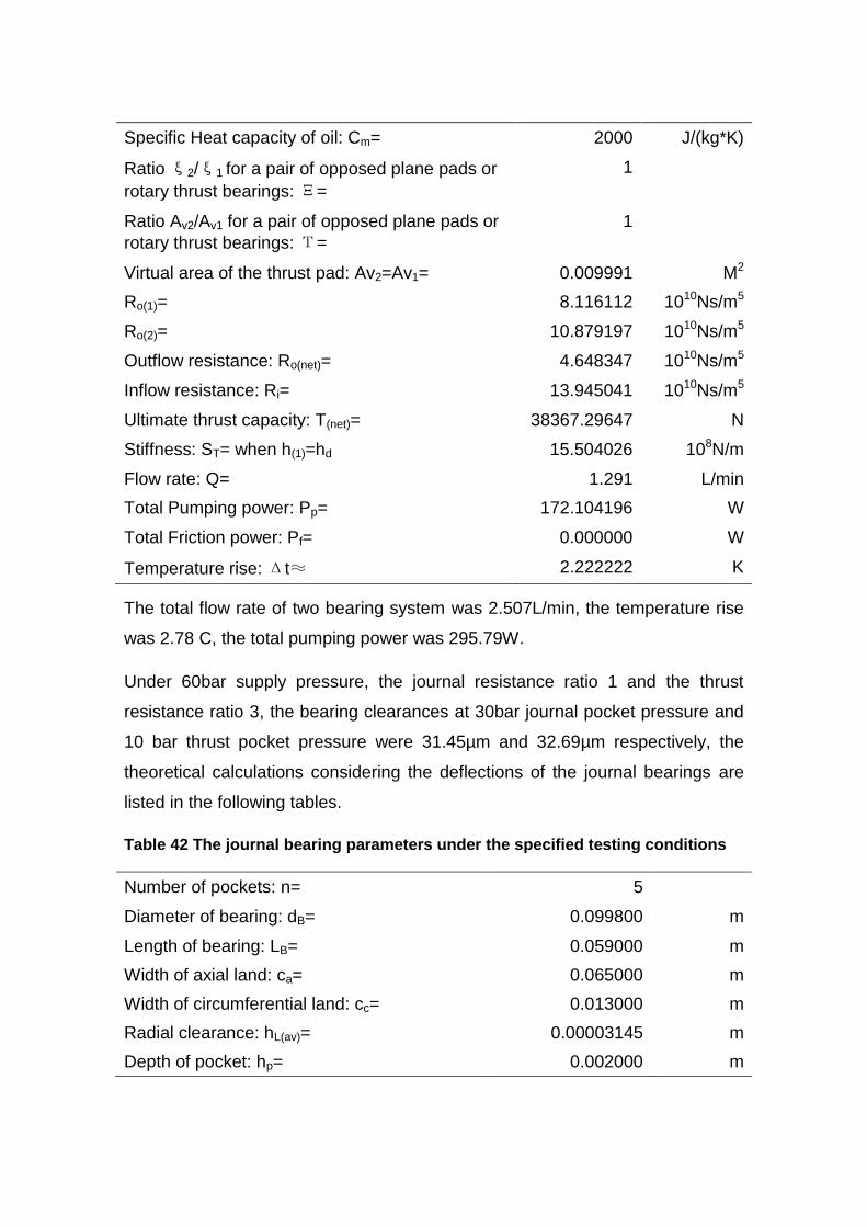
Specific Heat capacity of oil: Cm= 2000 J/(kg*K)
Ratio ξ2/ξ1 for a pair of opposed plane pads or
rotary thrust bearings: Ξ=
1
Ratio Av2/Av1 for a pair of opposed plane pads or
rotary thrust bearings: Τ=
1
Virtual area of the thrust pad: Av2=Av1= 0.009991 M2
Ro(1)= 8.116112 1010Ns/m5
Ro(2)= 10.879197 1010Ns/m5
Outflow resistance: Ro(net)= 4.648347 1010Ns/m5
Inflow resistance: Ri= 13.945041 1010Ns/m5
Ultimate thrust capacity: T(net)= 38367.29647 N
Stiffness: ST= when h(1)=hd 15.504026 108N/m
Flow rate: Q= 1.291 L/min
Total Pumping power: Pp= 172.104196 W
Total Friction power: Pf= 0.000000 W
Temperature rise: Δt≈ 2.222222 K
The total flow rate of two bearing system was 2.507L/min, the temperature rise
was 2.78 C, the total pumping power was 295.79W.
Under 60bar supply pressure, the journal resistance ratio 1 and the thrust
resistance ratio 3, the bearing clearances at 30bar journal pocket pressure and
10 bar thrust pocket pressure were 31.45µm and 32.69µm respectively, the
theoretical calculations considering the deflections of the journal bearings are
listed in the following tables.
Table 42 The journal bearing parameters under the specified testing conditions
Number of pockets: n= 5
Diameter of bearing: dB= 0.099800 m
Length of bearing: LB= 0.059000 m
Width of axial land: ca= 0.065000 m
Width of circumferential land: cc= 0.013000 m
Radial clearance: hL(av)= 0.00003145 m
Depth of pocket: hp= 0.002000 m

Supply Pressure: p1= 6000000 Pa
Rotational speed: Nd= 0 rev/min
Resistance ratio: ξ= 1
Viscosity of oil: η= 15 cSt
Density of oil: ρ= 900 kg/m3
Specific Heat capacity of oil: Cm= 2000 J/(kg*K)
Constant: k= 0.937096
Bearing shape factor: Φ= 0.753099
Bearing shape factor: Ea= 0.559322
Bearing shape factor: Ec= 0.170315
Outflow resistance: Rod= 5399.995342 108Ns/m5
Inflow resistance: Ri= 5399.995342 108Ns/m5
Ultimate load capacity: Wu= 18176.168029 N
Radial stiffness: Sl= 8.029051 108N/m
Flow rate: Q= 1.663 L/min
Pumping power: Pp= 166.250143 W
Friction power: Pf= 0.000000 W
Temperature rise: Δt≈ 3.333 °C
Table 43 The thrust bearing parameters under the specified testing conditions
Outer diameter of thrust pad: DB= 0.176000 m
Outer diameter of annular pocket: DP= 0.163000 m
Inner diameter of annular pocket: dP= 0.133000 m
Inner diameter of thrust pad: dB= 0.120000 m
Clearance at the lands of each thrust pad at no load: hd=
0.00003269 m
Clearance at the pocket: hP= 0.002000 m
Supply pressure: p1= 4000000 Pa
Speed of rotation: n= 0 rev/min
Resistance ratio: ξ= 3
Viscosity of the fluid: η= 0.0135 Ns/m2
Density of oil: ρ= 900 kg/m3
Specific Heat capacity of oil: Cm= 2000 J/(kg*K)

Ratio ξ2/ξ1 for a pair of opposed plane pads
or rotary thrust bearings: Ξ=
1
Ratio Av2/Av1 for a pair of opposed plane pads
or rotary thrust bearings: Τ=
1
Virtual area of the thrust pad: Av2=Av1= 0.009991 M2
Ro(1)= 5.665750 1010Ns/m5
Ro(2)= 7.594623 1010Ns/m5
Outflow resistance: Ro(net)= 3.244949 1010Ns/m5
Inflow resistance: Ri= 9.734848 1010Ns/m5
Ultimate thrust capacity: T(net)= 38367.296470 N
Stiffness: ST= when h(1)=hd 13.753533 108N/m
Flow rate: Q= 1.849 L/min
Total Pumping power: Pp= 246.536986 W
Total Friction power: Pf= 0.000000 W
Temperature rise: Δt≈ 2.222222 K
From the tables above, the stiffness for journal bearing was 802.9N/µm, so the
Dh under 3000N maximum load was 3.736µm. The stiffness for thrust bearing
was 1375.4N/µm, so the Dh under 500N maximum load was 0.364µm.
6.4.3 THE EXPERIMENT RESULTS
6.4.3.1 THE POCKET PRESSURE
There are 7 pockets within the bearing housing. As shown in the following figure,
the seven pocket pressure measuring screws were on the top and two sides of
the bearing housing: 2 for thrust pockets and 5 for journal pockets.

Figure 75 Seven pocket pressure measuring screws
The required journal pocket pressure is 30bar and the resistance ratio for the
journal resistors is 1, so the supply pressure shall be adjusted as 60bar.
The required thrust pocket pressure is 10bar and the resistance ratio for the
thrust resistors is 3, so the supply pressure shall be 40bar.
But there was only one pump to supply both the journal bearings and the thrust
bearings. The supply pressure was 60bar. So a pressure regulating valve as
well as a pressure gauge was put before the thrust bearing inlet pipe. The
following two figures show the pipe connections and the schematic diagram of
the oil supply system.

Figure 76 The pipes and connections for the hydraulic system
Figure 77 The schematic diagram of the oil supply system
Thrust bearing regulating valve
Journal bearing pressure gauge
Thrust bearing pressure gauge
Thrust bearing pockets
Journal bearing pockets
Thrust bearing supply pipe
Journal bearing supply pipeSupply
pressure 60bar
Journal bearing pocket pressure
60bar
Thrust bearing pocket pressure
40bar
By using a thrust bearing regulating valve, the thrust bearing supply pressure
could be adjusted to 40bar. Under the new supply pressure combination of
journal bearing supply pressure of 60bar and thrust bearing supply pressure of
40bar, new pocket pressures without any loading conditions are listed below:
Pthrust1=6bar Pthrust2=7bar

Pjournal1=10bar
Pjournal2=17.5bar Pjournal4=16bar
Pjournal3=11bar Pjournal5=13bar
The starting force to rotate the bearing spindle under this uneven journal pocket
pressures was 0.1N as showed in the following figure.
Figure 78 The start rotating force of the bearing spindle under uneven journal
bearing pocket pressures
According to the supply pressure and the resistance ratio, the pocket pressure
shall be 10bar in thrust and 30bar in journal respectively. The actual pressures
were all lower than the target pressures.
Although the bearing restrictors were nominally same as one specified type, the
actual manufacturing process seemed not that ideal. Since the inner diameter of
the tube was very small, about 0.3mm, and the inner diameter was strongly
relevant to the resistance of the hydrostatic bearing restrictors. Any slight
reduce or increase of the inner diameter could cause different resistance value.
The inner diameter of the restrictor tube might vary slightly, which would finally
lead to different resistance ratio of the journal bearing.
Another reason was that there was only one journal bearing inlet pipe and this
pipe supplied all the five journal bearings. Five different journal restrictors had
different distance to the supply point and the paths conducting the oil flow within

the housing were different from each other. The pressure drop in pipes was
mainly caused by:
Friction;
Elevation difference;
Changes of kinetic energy due to the shape of the paths;
The pressure drop in circular pipes could be calculated by the equation below:
Pressure drop equation
Equation 34
Where l is pipe friction coefficient, v is flow velocity.
Also according to Bernoulli’s Equation below:
Bernoulli’s Equation
Equation 35
When the elevation h keeps constant, the higher the flow rate is, the lower the
pressure will be. Ideally, each journal pocket has the same pocket pressure. But
the actual condition was that the flow rate of each pocket was different due to
different bearing gaps. The different outflow resistance of each journal pocket
led to different pocket pressure.
In this case, the frictional force within the flow paths was the main source of the
pressure drop. The paths’ difference would lead to different actual supply
pressure for each restrictor on the inlet side.
So swapping the nearer restrictor with a larger resistance restrictor and the
farther restrictor with a smaller resistance restrictor might be a simple solution.
The method was to keep swapping the restrictors of the highest pocket
pressure and the lowest pocket pressure to adjust the five bearing pocket
pressures until reaching an even condition.
After swapping the highest pressure journal restrictor and the lowest pressure
journal restrictor, the pocket pressures changed to the data below:
Pthrust1=7bar Pthrust2=7bar
Pjournal1=15bar

Pjournal2=17bar Pjournal4=17bar
Pjournal3=16bar Pjournal5=15bar
The starting force to rotate the bearing spindle under this uneven journal pocket
pressures was 0.05N as showed in the following g figure.
Figure 79 The start rotating force of the bearing spindle under even journal
bearing pocket pressures
It was initially concluded that the even journal pocket pressure could lead to
less internal frictional force to make the system more efficient.
The target pocket pressure is 30bar for journal bearings and 10bar for thrust
bearings, the solution to attain higher pocket pressure was to either increase
the motor power or change the shape of the restrictors to get the ideal
resistance ratio.
Another solution was to supply each pocket separately with an independent
close-loop-control pressure regulating valve to keep the pocket pressure on the
target value. As a result, its cost would be much higher than the original design.
The journal bearing pocket pressure increased a lot after changing the journal
restrictors to lower resistance, and by increasing thrust supplying pressure, the
thrust bearing pocket pressure also increased. The improved value is showed in
the following:

Pthrust1=8bar Pthrust2=8bar
Pjournal1=27bar
Pjournal2=25bar Pjournal4=25bar
Pjournal3=27bar Pjournal5=25bar
This pocket pressure distribution was almost close to the target pressure
combination: Pjournal=30bar and Pthrust=10bar. Since the fuse in the plug of the
inverter was 3A, when the working frequency of the plug reached 50Hz, the
fuse blew and the system broke down. So the target supply pressure could not
be realized by this set of inverter and motor.
6.4.3.2 THE FLOW RATE
There were two oil inlet pipes connected to the housing of the bearing system.
Since these two pipes were high pressure pipes, the flow rate was not safe by
being measured through high pressure pipes.
There were also two outlet pipes of the bearing system. Most of the oil from the
bearing pockets flowed through these two pipes into the oil tank. However there
was still some oil flowing through the bearing gap and drops to the workbench
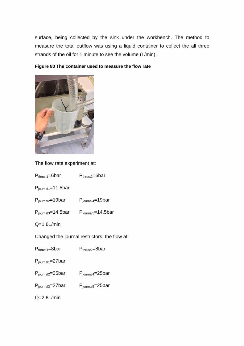
surface, being collected by the sink under the workbench. The method to
measure the total outflow was using a liquid container to collect the all three
strands of the oil for 1 minute to see the volume (L/min).
Figure 80 The container used to measure the flow rate
The flow rate experiment at:
Pthrust1=6bar Pthrust2=6bar
Pjournal1=11.5bar
Pjournal2=19bar Pjournal4=19bar
Pjournal3=14.5bar Pjournal5=14.5bar
Q=1.6L/min
Changed the journal restrictors, the flow at:
Pthrust1=8bar Pthrust2=8bar
Pjournal1=27bar
Pjournal2=25bar Pjournal4=25bar
Pjournal3=27bar Pjournal5=25bar
Q=2.8L/min

The flow rate increased quite a lot due to the increased supply pressure.
According to the theoretical calculation at Pthrust=10bar and Pjournal=30bar:
Journal clearance was 28.5µm, the deflection at 30bar was 2.952µm, the
h’=31.452µm, the total theoretical flow rate (30bar, 15cSt, 5 journal pockets)
was 1.216L/min.
Thrust clearance was 29.0µm, the deflection at 10bar was 3.691µm, the
h’=32.691µm, the total theoretical flow rate (10bar, 15cSt, 2 thrust pockets) was
1.849L/min.
The total flow rate of the system was 3.065L/min, which was quite near the
second experimental data, 2.8L/min. If the pocket pressure could reach 30bar
and 10bar ideally, the actual flow rate would probably be around 3L/min.
The increased flow rate at the same supply pressure also led to the higher
pumping power of the motor. The temperature rise tests of the system would be
illustrated in the following section.
6.4.3.3 THE AXIAL STIFFNESS
The axial stiffness could be measured when the bearing was lying on the
workbench. The working load of the thrust bearing was 50KG. So 500N weights
were used to do the tests.
Figure 81 Lying down the bearing housing to measure the axial stiffness

Figure 82 The sensor of the clock fixed on the top face of the bearing housing
Figure 83 The schematic diagram of the axial stiffness testing system
Oil TankPump
Work Bench
Bearing Housing
5KG
5KG
5KG
5KG
5KG
5KG
Bearing Housing

The following tables and figures were the two sets of data of the experiments to
measure the axial stiffness of the hydrostatic bearing system:
Table 44 The table of axial stiffness test 1 of the bearing system (Pjournal1=9bar,
Pjournal2=17bar, Pjournal3=13bar, Pjournal4=18bar, Pjournal5=12bar, Pthrustfront=5bar,
Pthrustrear=5bar)
Weight (KG) Displacement (µm) Stiffness (N/µm)
10.6 0.5 21.2
20.6 5 41.2
25.6 8 32
30.6 10 30.6
25.6 10 25.6
20.6 8 25.8
10.6 3 35.3
0 1
Figure 84 The figure of axial stiffness test 1 of the bearing system (Pjournal1=9bar,
Pjournal2=17bar, Pjournal3=13bar, Pjournal4=18bar, Pjournal5=12bar, Pthrustfront=5bar,
Pthrustrear=5bar)

Table 45 The table of axial stiffness test 2 of the bearing system (Pjournal1=9bar,
Pjournal2=17bar, Pjournal3=13bar, Pjournal4=18bar, Pjournal5=12bar, Pthrustfront=5bar,
Pthrustrear=5bar)
Weights (KG) Displacement (µm) Stiffness (N/µm)
10.6 1.6 66.3
21.1 3.0 70.3
35.6 5.0 71.2
40.6 8.0 50.8
50.6 11.0 46.0
40.6 9.7 41.9
35.6 4.2 84.8
21.1 4.5 46.9
10.6 1.5 70.7
Table 46 The figure of axial stiffness test 2 of the bearing system (Pjournal1=9bar,
Pjournal2=17bar, Pjournal3=13bar, Pjournal4=18bar, Pjournal5=12bar, Pthrustfront=5bar,
Pthrustrear=5bar)
During the loading and unloading process of the axial stiffness tests, the
displacement data showed some consistency with the weights change. But the
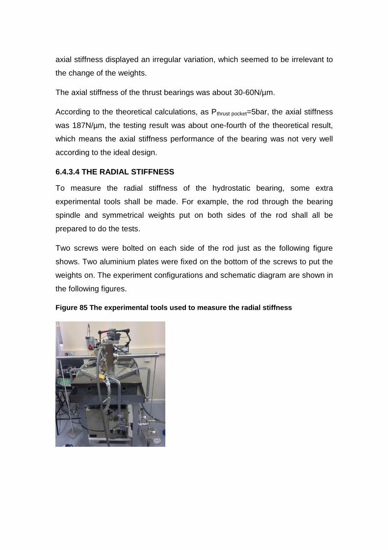
axial stiffness displayed an irregular variation, which seemed to be irrelevant to
the change of the weights.
The axial stiffness of the thrust bearings was about 30-60N/µm.
According to the theoretical calculations, as Pthrust pocket=5bar, the axial stiffness
was 187N/µm, the testing result was about one-fourth of the theoretical result,
which means the axial stiffness performance of the bearing was not very well
according to the ideal design.
6.4.3.4 THE RADIAL STIFFNESS
To measure the radial stiffness of the hydrostatic bearing, some extra
experimental tools shall be made. For example, the rod through the bearing
spindle and symmetrical weights put on both sides of the rod shall all be
prepared to do the tests.
Two screws were bolted on each side of the rod just as the following figure
shows. Two aluminium plates were fixed on the bottom of the screws to put the
weights on. The experiment configurations and schematic diagram are shown in
the following figures.
Figure 85 The experimental tools used to measure the radial stiffness

Figure 86 The schematic diagram of the radial stiffness testing system
5KG
5KG
5KG
5KG
5KG
5KGOil TankPump
Bearing Housing
Work Bench
Rod
Figure 87 The weights used to load the system

Figure 88 Stack same weights on both sides of the rod at the same time
Table 47 Front thrust plate displacement measurement

Table 48 Rear thrust plate displacement measurement
Table 49 Radial stiffness test 1
Weights (KG)
Front thrust plate displacement (µm)
Front stiffness (N/µm)
Rear thrust plate displacement (µm)
Rear stiffness (N/µm)
4.5 2.0 45.4 -1.0 -90.8
9.0 -0.5 -360.0 -0.5 -360.0
13.5 1.0 270.0 -3.0 -90.0
18.5 1.0 370.0 -3.0 -123.3
23.5 -3.0 -156.7 -4.0 -117.5
18.5 -3.0 -123.3 -3.0 -123.3
13.5 1.0 270.0 -4.0 -67.5
9.0 -4.0 -45.0 -4.0 -45.0
4.5 -3.0 -30.0 -4.0 -22.5
0.0 -2.0 0.0 -2.0 0.0

Figure 89 The figure of radial stiffness test 1
Table 50 Radial stiffness test 2
Weights (KG)
Front thrust plate displacement (µm)
Front stiffness (N/µm)
Rear thrust plate displacement (µm)
Rear stiffness (N/µm)
4.5 3.0 30.3 -1.0 -90.8
9.0 -2.5 -72.0 0.0
13.5 3.0 90.0 -1.0 -270.0
18.5 -3.0 -123.3 -1.0 -370.0
23.5 -3.0 -156.7 -2.8 -167.9
18.5 -1.5 -246.7 -3.0 -123.3
13.5 2.0 135.0 -2.0 -135.0
9.0 -1.0 -180.0 -3.0 -60.0
4.5 1.5 60.0 -2.8 -32.1
0.0 1.8 0.0 1.0 0.0

Table 51 The figure of radial stiffness test 2
Table 52 Radial stiffness test 3
Weights (KG)
Front thrust plate displacement (µm)
Front stiffness (N/µm)
Rear thrust plate displacement (µm)
Rear stiffness (N/µm)
4.5 0.0 -1.8 -50.4
9.0 3.0 60.0 -3.5 -51.4
13.5 2.5 108.0 -4.2 -64.3
18.5 1.5 246.7 -2.8 -132.1
23.5 -1.2 -391.7 -4.0 -117.5
18.5 2.5 148.0 -5.0 -74.0
13.5 1.5 180.0 -5.0 -54.0
9.0 -1.0 -180.0 -5.0 -36.0
4.5 1.5 60.0 -5.0 -18.0
0.0 -3.0 0.0 -1.0 0.0

Table 53 The figure of radial stiffness test 3
The positive value of the displacement meant an upward movement of the edge
of the thrust pad, which was an abnormal phenomenon. The normal result
should be all negative values to indicate the downward movements of both
edges of the opposite thrust pads.
From the data, the rear stiffness was always negative, which meant the
displacement of the rear thrust plate was always downwards. But the movement
of the front thrust plate was quite irregular. Its direction fluctuated with different
weights. The poor tilting performance of the hydrostatic bearing system was
probably the reason of it.
From all the data above, the average radial stiffness of the hydrostatic bearing
system was about 100N/µm.
According to the theoretical calculations, as Pjournal pocket=27bar, the axial
stiffness was 361N/µm, the testing result was about one-third of the theoretical
result, which meant the radial stiffness performance of the bearing was not very
well according to the ideal design.

6.4.3.5 THE TEMPERATURE RISE
The energy used to increase the temperature mainly came from two sources:
pumping power and frictional power. The over temperature rise would cause the
malfunction of the bearing system.
To test the relationship between the pumping power and the temperature rise,
the bearing spindle was set as a stationary status, i.e. N=0rpm. If only the
pumping power was high enough to raise the oil temperature, then the cooling
system was necessary before doing the rotational tests.
The following table was used to show the temperature rise due to the pumping
power only within 60 minutes.
Pjournal supply=60bar Pthrust supply=40bar
ŋ=15cSt N=0rpm Troom=22.8°C
Pthrust front=7bar Pthrust rear=7bar
Pjournal1=17bar
Pjournal2=20bar Pjournal4=17bar
Pjournal3=15bar Pjournal5=20bar
Table 54 The temperature rise condition under stationary pumping condition and
lower pocket pressure
T(min) Tai0(°C) Tai1(°C) Tai2(°C) Tai3(°C)
0 23.9 22.3 22.3 23.9
10 24.6 23.9 23.9 24.6
15 25.5 25.0 25.5 25.2
20 25.9 25.8 25.8 25.9
25 26.5 26.5 26.5 26.4
30 27.0 27.0 27.1 26.9
35 27.6 27.7 27.8 27.5
40 28.1 28.2 28.1 27.9
45 28.6 28.8 28.9 28.5

50 29.1 29.4 29.4 29.0
55 29.4 29.7 29.8 29.2
60 29.8 30.1 30.2 29.6
Figure 90 The temperature rise condition under stationary pumping condition
and lower pocket pressure
The theoretical temperature rises considering the deflection of the bearing
surface at Pjournal pocket=18bar and Pthrust pocket=7bar were:
ΔTthrust=1.6ºC
ΔTjournal=2.0ºC
From the testing data, the temperature keeps rising. The temperature rise was
below 3ºC during the first 30 minutes. After the pump’s continuous work, the
temperature continuously rose and reached about 30ºC in 60 minutes.
After changing five journal restrictors from high resistance to low resistance, the
pocket pressure increased. The condition was listed below:
Pjournal supply=60bar Pthrust supply=40bar
ŋ=15cSt N=0rpm Troom=22.8°C
Time (min)
Tem
pe
ratu
re (
ºC)

Pthrust front=8bar Pthrust rear=8bar
Pjournal1=27bar
Pjournal2=25bar Pjournal4=25bar
Pjournal3=27bar Pjournal5=25bar
Table 55 The temperature rise condition under stationary pumping condition and
higher pocket pressure
T(min) Tai0(°C) Tai1(°C) Tai2(°C) Tai3(°C)
0 24.3 23.5 23.5 24.3
5 25.9 26.0 26.1 26.0
10 27.6 27.3 27.5 27.6
15 28.4 28.5 28.5 28.4
20 29.2 29.1 29.3 29.2
25 29.5 29.6 29.7 29.5
30 29.9 29.8 30.0 29.9
35 30.4 30.3 30.5 30.4
40 30.8 30.8 31.0 30.9
45 31.4 31.7 31.7 31.5
50 32.0 32.0 32.3 32.2
55 32.6 32.5 32.8 32.9

Figure 91 The temperature rise condition under stationary pumping condition
and higher pocket pressure
The theoretical temperature rose considering the deflection of the bearing
surface at Pjournal pocket=26bar and Pthrust pocket=8bar were:
ΔTthrust=1.8ºC
ΔTjournal=2.9ºC
From the testing data, the temperature kept rising. The temperature rise was
below 3ºC during the first 30 minutes. After the pump’s continuous work, the
temperature continuously rose and reached about 33ºC in 60 minutes.
Also from the data, the temperature rise at higher pocket pressure was larger
than the temperature rise at lower pocket pressure. In a lower resistance
hydrostatic bearing system, to maintain the same supply pressure meant the
increase of the supply power because the flow rate increased a lot. Since it was
a stationary system, all the energy raising the temperature came from the
pumping power.
So, if the pumping power increases, the temperature rise will also increase. The
highest temperature rise was about 10°C, which greatly beyond the required
Tem
pe
ratu
re (
ºC)
Time (min)

temperature rise. So a chilling system was definitely needed to cool down the oil
as well as a large oil tank was needed to maintain the oil at a lower
temperature.


7 RESULTS AND DISCUSSION
According to experiment design, the target supply pressures were Pthrust=10bar
and Pjournal=30bar. Adjusted the size of the restrictors, the optimum supply
pressures were obtained as:
Pthrust1=8bar Pthrust2=8bar
Pjournal1=27bar
Pjournal2=25bar Pjournal4=25bar
Pjournal3=27bar Pjournal5=25bar
The fuse in the plug blew when the frequency of the invertor exceeded 50Hz, so
the highest safe supply pressures under this condition were 60bar for the
journal bearings and 40bar for the thrust bearings. The test results based on
this combination of pocket pressures could be used to analyse the comparison
between the theoretical calculations and actual experimental results.
The reasons of uneven journal bearing pocket pressures at the same supply
pressure were probably the following two points:
1. The slight manufacturing difference, including the burs remained within
the tube or the different straightness of the hypodermic needles from
different bearing restrictors, led to the different resistance ratio of the
bearing restrictors;
2. Different oil conducting paths of each bearing pocket led to different
pressure drop through different paths. Because of the manufacturing
technique of drilling the holes inside the bearing housing to make the oil
paths, the angles of two straight drills would cause the oil flow lose its
kinetic energy when flowing through the angle and will lead to the extra
pressure drop through the oil path. Different shapes of the oil paths
would have different influences on the pressure drop of each journal
bearing pockets.

According to the reasons listed above, the simply solution was to swapping the
restrictors of the highest pocket pressure and the lowest pocket pressure and
repeat this procedure until all the journal pocket pressures equal to each other.
And another advanced solution might be using the 3D-printing technology to
manufacture the oil path inside the bearing housing more smooth, which means
not any sharp drill angles on the oil paths. By using the 3D-printing technology,
each oil path of the five journal bearing pockets will have the same and
minimum pressure drop condition by designing each path smoothly and
separately.
The flow rate at higher pocket pressures was 2.8L/min, and the theoretical flow
rate was 3.1L/min. So the experimental results were quite accord with the
theoretical results. The close values probably meant the actual bearing gap was
quite close to the design bearing gap. From the last measurement by the CMM
machine, the final bearing gap was 24.955µm, which quite accorded with the
target bearing gap of about 25µm. So the diamond turning process complied
quite well with the design requirement.
The experimental axial stiffness, 30-60N/µm, was about one-fourth of the
theoretical value, 187N/µm, and the radial stiffness, 80-100N/µm, was about
one-third of the theoretical value, 361N/µm. The error between the theoretical
values and actual values were quite large mainly due to the poor tilting
performance of the bearing system. The single pocket thrust plate was easy for
manufacturing which also meant lower cost, but it had relatively lower tilting
stiffness compared with the multi-pockets design. If a high tilting stiffness was
needed, the hydrostatic bearing system should be designed to meet the specific
demand. In this R2R manufacturing system, since a couple of symmetrical
hydrostatic bearings are used to put the 300KG drum roll on, most of the load
comes from the gravity of the drum with its direction towards the ground, there
is almost no tilting force or torque on the hydrostatic bearing shaft. And the total
gravity force is distributed evenly on the two bearing spindles without too much
irregular motions. So in this research project, the tilting stiffness is not regarded
as the important working parameter for the bearing system. On the other side,

the radial stiffness to balance the gravitational force on the spindle is one of the
crucial properties of the hydrostatic bearing system.
The experimental temperature rise just under the static condition, i.e. no
rotational speed, continued to rise before turning off the pump. After one hour
operation time, the oil temperature rise within the system was about 10ºC.
According to the analysis before, the temperature rise over 3ºC was not well
recommended, so a cooling system was definitely required to lower the
temperature of the hydrostatic bearing system. The temperature control was
beneficial not only to the accuracy of the bearing spindle, but also to the life
cycle of the hydrostatic bearing system in a long term as well.
According to Figure 71 The delamination and scratches condition on the surface
of the thrust plate, after short operational tests, the scratches on the surface
were just about 0.1µm, and it probably came from the friction between the
remained burs and the bearing surfaces. The delamination conditions showed
in the figure were quite obvious that the burs drop easily at high rotational
speed and cause the extra attrition between the surfaces of the hydrostatic
bearings. The depth of the scratches was quite small that it could almost be
considered as no extra attrition during the normal operational process. But the
quality of the nickel-based electroless coating was definitely needed to be
improved to eliminate the delamination degradation phenomenon and
strengthen the surface mechanical properties such as hardness. If the coating is
cheap and perfect, the new R2R hydrostatic bearing system might be
economically successful and will definitely have a broad application.


8 CONCLUSIONS AND FURTHER WORKS
Measured performance in terms of lubricant temperature rise, flow rate was in
close agreement with the predictions from the theoretical calculations.
Axial stiffness and radial stiffness were measured by amplifiers by adding
symmetrical weights on both sides of the system. Since the fluctuation of the
values of both axial stiffness and radial stiffness were quite large, the reasons of
the deviation of the stiffness were needed to be further analysed by both
theoretical analysis and experimental testing works. The reasons might be due
to the design features as well as the manufacturing accuracy.
The tilt stiffness of the bearing system was not satisfied, so the rotational tests
were not recommended to proceed due to the irregular rotational movement will
cause some extra attrition to the surface of the bearing spindle. The low tilt
stiffness could not prevent the contact of the surfaces by the force of the
irregular rotational torque. So the 300rpm test shall be performed when the tilt
stiffness is improved in the future. And a cooling system is needed to protect the
system from the overheat condition.
The equations in the book (Stansfield, 1970, Hydrostatic bearings for machine
tools and similar applications) only use some basic parameters of the
hydrostatic bearing systems, such as the radial clearance, the dimensions of
the shaft and the pocket, the viscosity of the lubricant, the rotational speed, the
supply pressure, the density of the oil, the specific heat capacity of the oil, etc.,
and some advanced parameters were not included into the calculation process,
such as centripetal acceleration when one bearing surface is rotated in a very
high speed for an externally pressurized thrust bearing (Srinivasan, 2013a).
All the equations were based on the assumption that all the flow within the
hydrostatic bearing systems is laminar, so some complex static and dynamic
conditions inside the bearing systems during the operational process were not
been analysed in the initial review report. All the typical parameters of the
hydrostatic system, such as outflow resistance, inflow resistance, ultimate load
capacity, radial stiffness, flow, pumping power, frictional power, and

temperature rise, were calculated without a velocity dependency. The geometry
of the hydrostatic bearing pockets and their restrictors were optimized by using
the time continuous pressure distribution at the bearing pocket, the laminar flow
behaviour and the constant velocity of the bearing (Srinivasan, 2013a). The
dynamic effects of the flow at high velocities within the pockets and the space
between the shaft and the bearing were not considered.
The best hydrostatic bearing design has higher load capacity, higher stiffness,
lower flow rate, lower energy consumption, and lower manufacturing cost. In the
next step, hydrostatic bearings experiments will probably be designed to real-
timely monitor the pocket pressure, flow rate, temperature change of the system.
The environmental conditions, such as temperature of the environment, dust
and dirt in the surrounding air, moisture and corrosive conditions, can also
affect a bearing’s performance adversely. Both mechanical and environmental
factors may affect the choice of a bearing and its performance. The more
complex the system is, the more important it is to consider all of its real
operational conditions, and then select the most suitable bearing type and its
features as well the proper lubricant type (Srinivasan, 2013b).

APPENDICES
Appendix A THE CODES FOR AUTOMATIC
CALCULATION EXCEL SPREADSHEET
A.1 CODES FOR HYDROSTATIC JOURNAL BEARINGS
Table A-1 Codes for hydrostatic journal bearings
Parameters Codes to calculate the parameters
Number of pockets: n= =B3
Diameter of bearing: dB= =B4
Length of bearing: LB= =B5
Width of axial land: ca= =B6
Width of circumferential land: cc= =B7
Radial clearance: hL(av)= =B8
Depth of pocket: hp= =B9
Supply Pressure: p1= =B10
Rotational speed: Nd= =B11
Resistance ratio: ξ= =B12
Viscosity of oil: η= =B13
Density of oil: ρ= =B14
Specific Heat capacity of oil: Cm= =B15
Constant: k= =1-4*B8/B9
Bearing shape factor: Φ= =B5/(3.14*B4/4)
Bearing shape factor: Ea= =(B5-2*B7)/B5
Bearing shape factor: Ec= =1-B6/(3.14*B4/4)
Outflow resistance: Rod= =0.75*B3*B13*B17*(1-B18)/B8/B8/B8/POWER(10,8)
Inflow resistance: Ri= =B20*B12
Ultimate load capacity: Wu=
=1.47*B12*B17*(1-B19)*(1+B18)*B10*B4*B4/(B12*(B12+0.4)*B17*B17*B18*(1-B18)+0.642*(B12+0.207)*(B12+6.02)*(1-B19))
Radial stiffness: Sl= =1.5*B12*B17*(1+B18)*B10*B4*B4/(B8*(1+B12)*(1+B12)*(1+(0.5*B12*B17*B17*B18*(1

-B18))/((1+B12)*(1-B19))))/POWER(10,8)
Flow: Q= =1.33*B10*B8*B8*B8/(B13*B17*(1+B12)*(1-B18))*POWER(10,6)
Pumping power: Pp= =1.33*B10*B10*B8*B8*B8/(B17*B13*(1+B12)*(1-B18))
Frictional power: Pf=
=0.00677*B17*B13*POWER(B4,4)*POWER(B11,2)*(1-B16*B18*B19)*(1+0.25*B16*B18*(1-B19)*(B3-4)/(1-B16*B18*B19))/B8
Temperature rise: Δt≈ =(B10+B26/(B24*POWER(10,-6)))/(B14*B15)

A.2 CODES FOR HYDROSTATIC THRUST BEARINGS
Table A-2 Codes for hydrostatic thrust bearings
Parameters Codes to calculate the parameters
Outer diameter of thrust pad: DB= =B3
Outer diameter of annular pocket: DP=
=B4
Inner diameter of annular pocket: dP=
=B5
Inner diameter of thrust pad: dB= =B6
Clearance at the lands of each thrust pad at no load: hd=
=B7
Clearance at the pocket: hP= =B8
Supply pressure: p1= =B9
Speed of rotation: n= =B10
Resistance ratio: ξ= =B11
Viscosity of the fluid: η= =B12
Density of oil: ρ= =B13
Specific Heat capacity of oil: Cm= =B14
Ratio ξ2/ξ1 for a pair of
opposed plane pads or rotary
thrust bearings: Ξ=
=B16
Ratio Av2/Av1 for a pair of opposed plane pads or rotary
thrust bearings: Τ=
=B17
Virtual area of the thrust pad: Av2=Av1=
=3.14*(B3*B3-B4*B4)/LN(B3/B4)/8-3.14*(B5*B5-B6*B6)/LN(B5/B6)/8
Ro(1)= =6*B12*LN(B3/B4)/3.14/B7/B7/B7*POWER(10,-10)
Ro(2)= =6*B12*LN(B5/B6)/3.14/B7/B7/B7*POWER(10,-10)
Outflow resistance: Ro(net)= =B20*B21/(B20+B21)
Inflow resistance: Ri= =B11*B22
Ultimate thrust capacity: T(net)= =B9*POWER(10,6)*B19*(1-B17/(1+8*B16*B11))
Stiffness: ST= (when h(1)=hd) =B9*POWER(10,6)*B19/B7*(3*B11/((1+B11)*(1+B11))+3*B16*B17*B11/((1+B16*B11)*(

1+B16*B11)))*POWER(10,-8)
Flow: Q= =B9*POWER(10,6)/(B22*POWER(10,10)*(1+B11))*POWER(10,6)
Total Pumping power: Pp= =B9*POWER(10,6)*B26*POWER(10,-6)*2
Total Frictional power: Pf=
=2*(1.078*POWER(10,-3)*B12*B10*B10*(POWER(B3,4)-POWER(B4,4))/B7+1.078*POWER(10,-3)*B12*B10*B10*(POWER(B4,4)-POWER(B5,4))/B8+1.078*POWER(10,-3)*B12*B10*B10*(POWER(B5,4)-POWER(B6,4))/B7)
Temperature rise: Δt≈ =(B9*POWER(10,6)+B28/(B26*POWER(10,-6)))/(B13*B14)

Appendix B THE TABLES OF MATERIALS TO BE
TURNED BY DIAMOND
B.1 THE MATERIALS READILY MACHINABLE BY DIAMOND
TURNING
Table B-1 The materials readily machinable by diamond turning (Gerchman, 1986)
Plastics
Acetal Polypropylene
Acrylic Polystyrene
Nylon Zeonex
Polycarbonate
Metals
Aluminum and aluminium alloys Electroless nickel plating on other materials
Brass Silver
Copper Tin
Gold Zinc
Infrared crystals
Cadmium sulfide Potassium bromide
Cadmium telluride Potassium dihydrogen phosphate (KDP)
Calcium fluoride Silicon
Cesium iodide Sodium chloride
Gallium arsenide Tellurium dioxide
Germanium Zinc selenide
Lithium niobate Zinc sulfide

B.2 THE MATERIALS NOT READILY MACHINABLE BY
DIAMOND TURNING
Table B-2 The materials not readily machinable by diamond turning (Gerchman,
1986)
Silicon-based glasses and ceramics
Ferrous materials (steel, iron)
Beryllium
Titanium
Molybdenum
Nickel (except for electroless nickel plating)

Appendix C THE SPECIFICATIONS FOR SJ100
INVERTER
Figure C-1 The specifications for HITACHI SJ100 inverter


Appendix D THE SPECIFICATIONS FOR ABB M2AA 090
L-4 MOTOR
Figure D-1 The specifications for the ABB M2AA 090 L-4 motor

Appendix E THE SPECIFICATIONS FOR MILLIMAR 1200
IC COMPACT AMPLIFIER
Figure E-1 The specifications for Millimar 1200 IC compact amplifier

Appendix F THE SPECIFICATIONS FOR NI 9217 RTD
ANALOG INPUT C SERIES MODULE
The following specifications are typical for the range –40°C to 70°C unless
otherwise noted. All voltages are relative to COM unless otherwise noted.
All specifications given in °C are specific to 100Ωplatinum RTDs.
Input Characteristics
Table F-1 The specifications for NI 9217 RTD Analog input C series module
Number of channels 4 Analog input channels
ADC resolution 24 bits
Type of ADC Delta-sigma
Sampling mode Scanned
Measurement range
Temperature -200 to 850°C
Resistance 0 to 400Ω
Common-mode range
COM-to-earth ground ±250 Vrms
Channel-to-COM 50 mV
Conversion time
High-resolution mode 200 ms per channel
800 ms total for all channels
High-speed mode 2.5 ms per channel
10 ms total for all channels
Noise
High-resolution mode 0.003 °C
High-speed mode 0.02 °C
Excitation current 1 mA per channel
Noise rejection
Normal mode (50/60 Hz)
High-resolution mode 85 dB min
High-speed mode None

Temperature accuracy (including noise), 4-wire mode
Measured Value Typical (25 °C) Maximum (–40 to 70 °C)
-200 to 150 °C 0.15 °C 0.35 °C
150 to 850 °C 0.20 °C 1.0 °C
Temperature accuracy (including noise), 3-wire mode
Measured Value Typical (25 °C) Maximum (–40 to 70 °C)
-200 to 150 °C 0.20 °C 0.50 °C
150 to 850 °C 0.30 °C 1.0 °C
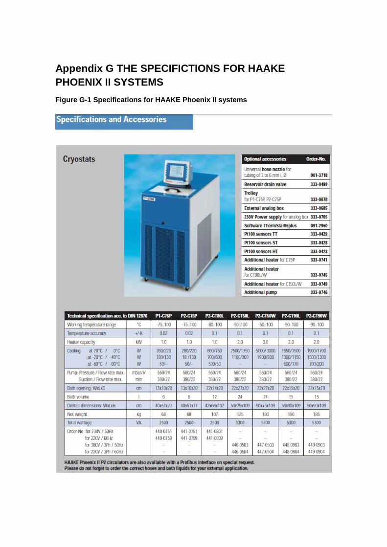
Appendix G THE SPECIFICTIONS FOR HAAKE
PHOENIX II SYSTEMS
Figure G-1 Specifications for HAAKE Phoenix II systems

Appendix H THE SPECIFICATIONS FOR LEMO FGG.00
TEMPERATURE MEASURING CONNECTOR
Table H-1 The specifications for LEMO FGG.00 temperature measuring connector
Manufacturer LEMO
Product Category B-Series Plugs and Receptacles
Product Type Connectors
Series 00
Shell Style Plug
Number of Contacts 4
Mounting Style Cable
Termination Style Solder
Current Rating 2 A
Brand LEMO
Contact Plating Copper, Nickel, Gold
Shell Plating Chrome
Factory Pack Quantity 150
Voltage Rating 700

Appendix I THE SPECIFICATIONS FOR TAYLOR-
HOBSON FORM TALYSURF-120L
Table I-1 The specifications for Taylor-Hobson form Talysurf-120L
Traverse Length 120mm
Traverse Speed 10mm/sec maximum
Measuring Speeds 1mm and 0.5mm/sec ±5%
Return Speed up to 5mm/sec
Gauge Type Phase Grating Interferometer, 1mN force nominal
Measuring Range 10mm
Resolution 12.8nm @ 10mm range
Range to Resolution Ratio 780,000:1
Straightness Accuracy 0.5µm over 120mm traverse
0.2µm over any 20mm traverse
Data Resolution 0.25µm
Dimensions (LxDxH) 396 x 127 x 195mm
Weight 11.5kg

REFERENCE
"Hydrostatic bearing design : J. P. O'Donoghue and W. B. Rowe, Tribology, 2 (1) (1969) 25–71; 68 figs., 4 tables, 10 refs.", (1969), Wear, vol. 13, no. 2, pp. 137.
"Electroless nickle composite coatings", (1997), Metal Finishing, vol. 95, no. 3, pp. 26.
Benga, G. C. and Abrao, A. M. (2003), "Turning of hardened 100Cr6 bearing steel with ceramic and PCBN cutting tools", Journal of Materials Processing Technology, vol. 143–144, no. 0, pp. 237-241.
Chen, D., Bonis, M., Zhang, F. and Dong, S. (2011), "Thermal error of a hydrostatic spindle", Precision Engineering, vol. 35, no. 3, pp. 512-520.
Chen, D., Fan, J. and Zhang, F. (2012), "Dynamic and static characteristics of a hydrostatic spindle for machine tools", Journal of Manufacturing Systems, vol. 31, no. 1, pp. 26-33.
Cheng, F., Jiang, S. and Liang, J. (2013), "Cavitation erosion resistance of microarc oxidation coating on aluminium alloy", Applied Surface Science, vol. 280, no. 0, pp. 287-296.
Cheng, K. and Rowe, W. B. (1995), "A selection strategy for the design of externally pressurized journal bearings", Tribology International, vol. 28, no. 7, pp. 465-474.
Cheng, K. and Shore, P. (2010), "Special issue on design of ultraprecision and micro machine tools and their key enabling technologies", International Journal of Machine Tools and Manufacture, vol. 50, no. 4, pp. 309.
De Pellegrin, D. V. and Hargreaves, D. J. (2012), "An isoviscous, isothermal model investigating the influence of hydrostatic recesses on a spring-supported tilting pad thrust bearing", Tribology International, vol. 51, no. 0, pp. 25-35.
Dumbrava, M. A. (1985), "Review of principles and methods applied to the optimum calculation and design of externally-pressurized bearings: Part 1: Low/moderate speed bearings", Tribology International, vol. 18, no. 3, pp. 149-156.
El-Sherbiny, M., Salem, F. and El-Hefnawy, N. (1984a), "Optimum design of hydrostatic journal bearings Part I: Maximum load capacity", Tribology International, vol. 17, no. 3, pp. 155-161.

El-Sherbiny, M., Salem, F. and El-Hefnawy, N. (1984b), "Optimum design of hydrostatic journal bearings Part II. Minimum power", Tribology International, vol. 17, no. 3, pp. 162-166.
Evans, C. and Bryan, J. B. (1991), "Cryogenic Diamond Turning of Stainless Steel", CIRP Annals - Manufacturing Technology, vol. 40, no. 1, pp. 571-575.
Forman, B. R., Gilles, H. L. and Faul, M. (2000), "Thermally induced bond failure of electroless nickel/IVD aluminum coatings deposited on steel", Surface and Coatings Technology, vol. 123, no. 2–3, pp. 106-111.
Gerchman, M. C. (1986), "SPECIFICATIONS AND MANUFACTURING CONSIDERATIONS OF DIAMOND MACHINED OPTICAL COMPONENTS.", Proceedings of SPIE - The International Society for Optical Engineering, Vol. 607, pp. 36.
Gu, L., Chen, X., Fan, X., Liu, Y., Zou, B., Wang, Y. and Cao, X. (2011), "Improvement of thermal shock resistance for thermal barrier coating on aluminum alloy with various electroless interlayers", Surface and Coatings Technology, vol. 206, no. 1, pp. 29-36.
Guo, Y. B. and Yen, D. W. (2004), "Hard turning versus grinding—the effect of process-induced residual stress on rolling contact", Wear, vol. 256, no. 3–4, pp. 393-399.
Ha, T., Lee, Y. and Kim, C. (2002), "Leakage and rotordynamic analysis of a high pressure floating ring seal in the turbo pump unit of a liquid rocket engine", Tribology International, vol. 35, no. 3, pp. 153-161.
HINO, M., MURAKAMI, K., MITOOKA, Y., MURAOKA, K. and KANADANI, T. (2009), "Effects of zincate treatment on adhesion of electroless Ni-P coating onto various aluminum alloys", Transactions of Nonferrous Metals Society of China, vol. 19, no. 4, pp. 814-818.
Kagnaya, T., Lambert, L., Lazard, M., Boher, C. and Cutard, T. (2014), "Investigation and FEA-based simulation of tool wear geometry and metal oxide effect on cutting process variables", Simulation Modelling Practice and Theory, vol. 42, no. 0, pp. 84-97.
Kazama, T. and Yamaguchi, A. (1993), "Optimum design of bearing and seal parts for hydraulic equipment", Wear, vol. 161, no. 1–2, pp. 161-171.
Kher, A. K. and Cowley, A. (1970), "An experimental investigation into the temperature effects in hydrostatic journal bearings", Tribology, vol. 3, no. 3, pp. 165-167.

König, W., Berktold, A. and Koch, K. -. (1993), "Turning versus Grinding – A Comparison of Surface Integrity Aspects and Attainable Accuracies", CIRP Annals - Manufacturing Technology, vol. 42, no. 1, pp. 39-43.
Lebeck, A. O. (1988), "Contacting mechanical seal design using a simplified hydrostatic model", Tribology International, vol. 21, no. 1, pp. 2-14.
Loxham, J. and Hemp, J. (1964), "The application of hydrostatic bearings to high precision machine tools", Production Engineer, vol. 43, no. 11, pp. 556-568.
Manojkumar, P. A., Gandhi, A. S., Kamaraj, M. and Tyagi, A. K. (2014), "Sliding wear behaviour of alumina coatings prepared from mechanically milled powders", Wear, vol. 313, no. 1–2, pp. 11-18.
Martin, J. K. (2004a), "Measured stiffness and displacement coefficients of a stationary rotor hydrostatic bearing", Tribology International, vol. 37, no. 10, pp. 809-816.
Martin, J. K. (2004b), "Measured stiffness and displacement coefficients of a stationary rotor hydrostatic bearing", Tribology International, vol. 37, no. 10, pp. 809-816.
Mayr, J., Jedrzejewski, J., Uhlmann, E., Alkan Donmez, M., Knapp, W., Härtig, F., Wendt, K., Moriwaki, T., Shore, P., Schmitt, R., Brecher, C., Würz, T. and Wegener, K. (2012), "Thermal issues in machine tools", CIRP Annals - Manufacturing Technology, vol. 61, no. 2, pp. 771-791.
Mekid, S. (2000), "High precision linear slide. Part I: design and construction", International Journal of Machine Tools and Manufacture, vol. 40, no. 7, pp. 1039-1050.
Moore, H. D. (1969), "Lubricating grease: Laboratory tests and their significance", Tribology, vol. 2, no. 1, pp. 11-17.
O'Donoghue, J. P. and Rowe, W. B. (1968), "Hydrostatic journal bearing (exact procedure)", Tribology, vol. 1, no. 4, pp. 230-236.
Osman, T. A., Safar, Z. S. and Mokhtar, M. O. A. (1991), "Design of annular recess hydrostatic thrust bearing under dynamic loading", Tribology International, vol. 24, no. 3, pp. 137-141.
Poli, M. (1975), "Dynamic behaviour of externally pressurized hydrostatic pads fed by throttling valves", Wear, vol. 31, no. 2, pp. 193-211.
Prabhu, T. J. and Ganesan, N. (1984), "Finite element application to the study of hydrostatic thrust bearings", Wear, vol. 97, no. 2, pp. 139-154.

Rowe, W. B. and Stout, K. J. (1972), "Viscosity variation in hydrostatic bearings", Tribology, vol. 5, no. 6, pp. 262-264.
Rudnik, E. and Jucha, T. (2013), "Electroless and electrolytic deposition of Co–SiC composite coatings on aluminum", Surface and Coatings Technology, vol. 232, no. 0, pp. 389-395.
Safar, Z. S. (1980), "Performance characteristics for the hydrostatic thrust bearing of a saw blade", Tribology International, vol. 13, no. 2, pp. 79-83.
Saxena, V., Rani, R. U. and Sharma, A. K. (2006), "Studies on ultra high solar absorber black electroless nickel coatings on aluminum alloys for space application", Surface and Coatings Technology, vol. 201, no. 3–4, pp. 855-862.
SHAO, J., DAI, C., ZHANG, Y., YU, X., XU, X. and WANG, Y. (2011), "The effect of oil cavity depth on temperature field in heavy hydrostatic thrust bearing", Journal of Hydrodynamics, Ser.B, vol. 23, no. 5, pp. 676-680.
Sharma, S. C., Jain, S. C. and Bharuka, D. K. (2002), "Influence of recess shape on the performance of a capillary compensated circular thrust pad hydrostatic bearing", Tribology International, vol. 35, no. 6, pp. 347-356.
Silva Mamede, N. F., Pinho Ramos, A. and Faria, D. M. V. (2013), "Experimental and parametric 3D nonlinear finite element analysis on punching of flat slabs with orthogonal reinforcement", Engineering Structures, vol. 48, no. 0, pp. 442-457.
Sinhasan, R., Sharma, S. C. and Jain, S. C. (1989), "Performance characteristics of an externally pressurized capillary-compensated flexible journal bearing", Tribology International, vol. 22, no. 4, pp. 283-293.
Sood, R., Guo, C. and Malkin, S. (2000), "Turning of Hardened Steels", Journal of Manufacturing Processes, vol. 2, no. 3, pp. 187-193.
Srinivasan, V. (2013a), "Analysis of Dynamic Load Characteristics on Hydrostatic Bearing with Variable Viscosity and Temperature using Simulation Technique", Indian Journal of Science and Technology, vol. 6, no. 6, pp. 4797-4803.
Srinivasan, V. (2013b), "Analysis of Static and Dynamic Load on Hydrostatic Bearing with Variable Viscosity and Pressure", Indian Journal of Science and Technology, vol. 6, no. 6.
Stansfield, F. M. (1970), Hydrostatic bearings for machine tools and similar applications, Machinery Publishing.

Sudagar, J., Lian, J. and Sha, W. (2013), "Electroless nickel, alloy, composite and nano coatings – A critical review", Journal of Alloys and Compounds, vol. 571, no. 0, pp. 183-204.
ZHANG, Y., FAN, L., LI, R., DAI, C. and YU, X. (2013), "Simulation and experimental analysis of supporting characteristics of multiple oil pad hydrostatic bearing disk", Journal of Hydrodynamics, Ser.B, vol. 25, no. 2, pp. 236-241.


![depl EVOLUTION Series def - ScameOnLine [EN] - … OR/GOLD 8766 2 CLOSER GANG For wall round box 8750 0 GANG 8751 1 GANG 8752 2 GANG 8753 3 GANG 8765 2 GANG For universal sockets 50](https://static.fdocuments.us/doc/165x107/5c65ee5309d3f230488b5d48/depl-evolution-series-def-scameonline-en-orgold-8766-2-closer-gang-for-wall.jpg)