Cranfield University Colin Clarke Development of an ... · Cranfield University Colin Clarke...
191
Cranfield University Colin Clarke Development of an automated identification system for nanocrystal encoded microspheres in flow cytometry. Cranfield Health PhD Thesis August 2008
Transcript of Cranfield University Colin Clarke Development of an ... · Cranfield University Colin Clarke...

Cranfield University
Colin Clarke
Development of an automated identification system for
nanocrystal encoded microspheres in flow cytometry.
Cranfield Health
PhD Thesis
August 2008

Cranfield University
Cranfield Health
Analytical Science and Informatics
Doctor of Philosophy
August 2008
Colin Clarke
Development of an automated identification system for nanocrystal encoded microspheres in flow cytometry.
Supervisor: Dr C.Bessant
August 2008
This thesis is submitted in partial fulfilment of the requirements of the Degree of PhD.
©Cranfield University, 2008. All rights reserved. No parts of this publication may be
reproduced without the written permission of the copyright holder.

Abstract
Colin Clarke ii Cranfield University
Abstract
Quantum dot encoded microspheres (QDEMs) offer much potential for bead based identification
of a variety of biomolecules via flow cytometry (FCM). To date, QDEM subpopulation
classification from FCM has required significant instrument modification or multiparameter
gating. It is unclear whether or not current data analysis approaches can handle the increased
multiplexed capacity offered by these novel encoding schemes. In this thesis the drawbacks of
currently available data analysis techniques are demonstrated and novel classification methods
proposed to overcome these limitations. A commercially available 20 code QDEM library with
fluorescent emissions at 4 distinct wavelengths and 4 different intensity levels was analysed using
flow cytometry. Multiparameter gating (MPG) a readily available classification method for
subpopulations in FCM was evaluated. A support vector machine (SVM) and two types of
artificial neural networks (ANNs), a multilayer perceptron (MLP) and probabilistic radial basis
function (PRBF) were also considered. For the supervised models rigorous parameter selection
using cross validation (CV) was used to construct the optimum models. Independent test set
validation was also carried out. As a further test, external validation of the classifiers was
performed using multiplexed QDEMs solutions.
The performance of MPG was poor (average misclassification (MC) rate = 9.7%) was a time
consuming process requiring fine adjustment of the gates, classifications made on the dataset
were poor with multiple classifications on single events and as the multiplex capacity increases
the performance is likely to decrease. The SVM had the best performance in independent test
validation with 96.33% accuracy on the independent testing (MLP = 96.12%, PRBF = 94.38%).
Furthermore the performance of the SVM was superior to both MPG and both ANNs for the
external validation set with an average MC rate for MLP = 6.1% and PRBF = 7.5% whereas the
SVM MC rate was 2.9%. Assuming that the external test solutions were homogenous the variance
between classified results should be minimal hence, the variance of correct classifications (CCs)
was used as an additional indicator of classifier performance. The SVM demonstrates the lowest
variance for each of the external validation solutions (average σ2 = 31479) some 50% lower than
that of MPG. As a conclusion to the development of the classifier, a user friendly software system
has been developed to allow construction and evaluation of multiclass SVMs for use by FCM
practitioners in the laboratory. SVMs are a promising classifier for QDEMs that can be rapidly
trained and classifications made in real time using standard FCM instrumentation. It is hoped that
this work will advance SAT for bioanalytical applications.

Acknowledgements
Colin Clarke iii Cranfield University
Acknowledgements
I would like to thank Conrad Bessant for his guidance and invaluable assistance
throughput the project.
I would also like to express my gratitude to my colleagues, Clair Gallagher and Sarah
Thiolett for their tireless endeavours in the laboratory.
Thanks to Mike Malecha and Selly Saini for their work in the early stages of this work.
Thanks to the members of the Cranfield Bioinformatics Group and Cranfield Health who
have assisted me during course of this project.
This work is dedicated to my parents Joe and Breda, and my brothers, Alan, Eoin and
David.
Abbreviations
Colin Clarke iv Cranfield University
Abbreviations
ANN artificial neural network RNA ribonucleic acid
ASO allele specific oligonucleotide S specificity
ASPE allele specific primer extension SAT suspension array technology
SEM scanning electron microscope
CCD charged couple detector SERRS surface enhanced Raman spectra
cDNA complementary DNA SMO sequential minimal optimization
CC rate correct classification rate SNP single nucleotide polymorphism
CoeffV coefficient of variation SSC side scatter
CV cross validation SV support vector
cvacc CV accuracy SVM support vector machine
DNA deoxyribonucleic acid testacc test set accuracy
ECOC error output coding TN true negative
FCM flow cytometry TOPO trioctylphosphine oxide
FCS flow cytometry standard TP true positive
FITC fluoroscein isothiocyanate trainacc train set accuracy
FN false negative TSC the SNP consortium
FP false positive YAG yttrium aluminium garnet
FSC forward scatter σ2 variance
FWHM full width half maximum
HIV human immunodeficiency virus
HLN hidden layer node
HT heat transfer
IQR interquartile range
LDA linear discriminant analysis
LSC laser scanning cytometry
LVQ learning vector quantisation
MC rate misclassification rate
MLP multilayer perceptron
MPG multiparameter gating
MS mass spectrometry
ODE octadecene
OLA oligonucleotide assay
OVO one versus one
OVR one versus rest
PCA principal component analysis
PCR polymerase chain reaction
PLSDA partial least squares discriminant analysis
PMT photomultiplier tube
PRBF probabilistic RBF
QD quantum dot
QDC quantum dot corporation
QDEM quantum dot encoded microsphere
R sensitivity
RBF radial basis function
RF radio frequency
RFID radio frequency identification tags
RMP Recurrent multilayer perceptron

Table of contents
Colin Clarke v Cranfield University
Table of contents
ABSTRACT.................................................................................................................................................. II
ACKNOWLEDGEMENTS .......................................................................................................................III
ABBREVIATIONS.....................................................................................................................................IV
TABLE OF CONTENTS ............................................................................................................................ V
LIST OF FIGURES .................................................................................................................................VIII
LIST OF TABLES ...................................................................................................................................XIII
CHAPTER 1: THESIS INTRODUCTION AND OVERVIEW ............................................................... 1
1.1 INTRODUCTION ..................................................................................................................................... 2 1.2 THESIS OVERVIEW................................................................................................................................. 5
CHAPTER 2: SUSPENSION ARRAY TECHNOLOGY ......................................................................... 6
2.1 OVERVIEW ............................................................................................................................................ 7 2.2 INTRODUCTION TO SUSPENSION ARRAY TECHNOLOGY .......................................................................... 7 2.3 ENCODING SCHEMES ........................................................................................................................... 12
2.3.1 Optical encoding ........................................................................................................................ 12 2.3.2 Nanocyrstal encoding................................................................................................................. 14 2.3.3 Non optical encoding schemes ................................................................................................... 18
2.4 MICROSPHERE SYNTHESIS, ENCODING AND BIO-CONJUGATION ........................................................... 20 2.5 DETECTION PLATFORMS...................................................................................................................... 24
2.5.1 Laser scanning cytometry........................................................................................................... 24 2.5.2 Microfluidic platforms................................................................................................................ 25 2.5.3 The Luminex system.................................................................................................................... 25 2.5.4 The Mosaic system...................................................................................................................... 27 2.5.5 Flow Cytometry .......................................................................................................................... 27
2.6 APPLICATIONS..................................................................................................................................... 28 2.6.1 SNP genotyping .......................................................................................................................... 29 2.6.2 Gene-expression ......................................................................................................................... 34 2.6.3 Proteomics.................................................................................................................................. 35
2.7 THESIS AIMS AND OBJECTIVES............................................................................................................. 37
CHAPTER 3: FLOW CYTOMETRIC ANALYSIS OF NANOCYRSTAL ENCODED
MICROSPHERES. ..................................................................................................................................... 39
3.1 OVERVIEW .......................................................................................................................................... 40 3.2 INTRODUCTION ................................................................................................................................... 40 3.3 FLOW CYTOMETER INSTRUMENTATION ............................................................................................... 42
3.3.1 Fluidics system ........................................................................................................................... 42 3.3.2 Excitation ................................................................................................................................... 43 3.3.3 Optics and detection................................................................................................................... 44 3.3.4 Electronics.................................................................................................................................. 47 3.3.5 The FCS filetype ......................................................................................................................... 49
3.4 APPLICATION OF A SUPERVISED FCM DATA ANALYSIS METHOD FOR QDEM CLASSIFICATION........... 50 3.4.1 Multiparameter gating. .............................................................................................................. 50 3.4.2 Materials and methods ............................................................................................................... 53 3.4.3 Results and discussion................................................................................................................ 57
3.5 IMPROVING ON MPG – THE CASE FOR RESEARCH................................................................................ 63

Table of contents
Colin Clarke vi Cranfield University
CHAPTER 4: SUPPORT VECTOR MACHINES FOR THE IDENTIFICATION OF QDEMS
FROM FCM DATA.................................................................................................................................... 65
4.1 INTRODUCTION ................................................................................................................................... 66 4.2 SUPPORT VECTOR MACHINES .............................................................................................................. 66
4.2.1 Supervised learning.................................................................................................................... 66 4.2.2 Fundamentals of support vector machines ................................................................................. 67 4.2.3 Multiclass support vector machines ........................................................................................... 72 4.2.4 Previous examples of SVM and flow cytometry data.................................................................. 75
4.3 MATERIALS AND METHODS ................................................................................................................. 76 4.3.1 SVM training data preparation .................................................................................................. 76 4.3.2 SVM implementation .................................................................................................................. 77 4.3.3 SVM model selection and training.............................................................................................. 77 4.3.4 SVM validation........................................................................................................................... 79
4.4 RESULTS AND DISCUSSION .................................................................................................................. 81 4.4.1 SVM parameter selection ........................................................................................................... 81 4.4.2 Outlier removal suitability ......................................................................................................... 85 4.4.3 Evaluation of multiclass SVM designs........................................................................................ 87 4.4.4 SVM performance with increasing QDEMs ............................................................................... 88 4.4.5 Independent testing set validation .............................................................................................. 90 4.4.6 Performance on the multiplexed testing sets .............................................................................. 92
4.5 CONCLUSION....................................................................................................................................... 94
CHAPTER 5: DEVELOPMENT OF A NEURAL NETWORK BASED QDEM CLASSIFICATION
SYSTEM...................................................................................................................................................... 97
5.1 OVERVIEW .......................................................................................................................................... 98 5.2 INTRODUCTION ................................................................................................................................... 98
5.2.1 Artificial neural networks........................................................................................................... 98 5.2.2 Previous applications in flow cytometry .................................................................................. 102
5.3 SELECTED ANN ARCHITECTURES ..................................................................................................... 103 5.3.1 Feed forward multilayer perceptrons....................................................................................... 104 5.3.2 Radial basis function networks................................................................................................. 107
5.4 MATERIALS AND METHODS ............................................................................................................... 111 5.4.1 Training data............................................................................................................................ 111 5.4.2 Multilayer perceptron implementation..................................................................................... 111 5.4.3 PRBF ANN implementation...................................................................................................... 111 5.4.4 Cross validation ....................................................................................................................... 112 5.4.5 Classifier testing and external validation................................................................................. 112
5.5 RESULTS AND DISCUSSION................................................................................................................ 113 5.5.1 ANN parameter selection ......................................................................................................... 113 5.5.2 Training and execution............................................................................................................. 116 5.5.3 Independent test set validation ................................................................................................. 116 5.5.4 Effect of increasing QDEMs on performance .......................................................................... 118 5.5.5 External validation ................................................................................................................... 120
5.6 CONCLUSION..................................................................................................................................... 123

Table of contents
Colin Clarke vii Cranfield University
CHAPTER 6: OVERALL DISCUSSION AND CONCLUSIONS. ...................................................... 125
6.1 OVERVIEW ........................................................................................................................................ 126 6.2 GENERAL DISCUSSION ....................................................................................................................... 126 6.3 FLOWSVM: A SOFTWARE PROGRAM FOR THE SVM CONSTRUCTION FOR THE CLASSIFICATION OF
QDEM FROM FCM DATA ....................................................................................................................... 135 6.3.1 Introduction.............................................................................................................................. 135 6.3.2 FlowSVM: FCM data plotting tool........................................................................................... 136 6.3.3 FlowSVM: SVM management module...................................................................................... 137
6.4 OVERALL CONCLUSION..................................................................................................................... 141 6.5 RECOMMENDATIONS FOR FUTURE WORK .......................................................................................... 143
BIBLIOGRAPHY..................................................................................................................................... 144
APPENDIX 1: FREQUENCY DIFFERENCE GATING AND PROBABILITY BINNING............. 162
APPENDIX 2: CONFUSION MATRICES. ........................................................................................... 167
SVM CONFUSION MATRIX ...................................................................................................................... 168 MLP CONFUSION MATRIX ...................................................................................................................... 169 PRBF CONFUSION MATRIX..................................................................................................................... 170
APPENDIX 3: QDEM SPECIFICATIONS ........................................................................................... 171
PRODUCT DATA SHEET ............................................................................................................................ 172 MATERIAL SAFETY DATA SHEET ............................................................................................................. 173
APPENDIX 4: CD CONTENTS.............................................................................................................. 175
List of figures
Colin Clarke viii Cranfield University
List of figures
FIGURE 1 STAGES OF A TYPICAL SAT ASSAY. FIRSTLY, A SUITABLE CODING SCHEME IS CHOSEN FOR THE
EXPERIMENT AND A NUMBER OF SETS OF DISTINCT MICROSPHERES ARE PRODUCED. CAPTURE MOLECULES
ARE ATTACHED TO EACH MICROSPHERE SET (E.G. OLIGONUCLEOTIDE). THE NEXT STAGE INVOLVES THE
HYBRIDISATION OF THE RESPECTIVE TARGET MOLECULES TO THE SPECIFIC MICROSPHERES (E.G. PCR
AMPLICONS). THE PRESENCE OF THE TARGET MOLECULE IS CONFIRMED VIA A HYBRIDIZATION SIGNAL, THE
IDENTITY OF THE MICROPSHERE (AND THEREFORE TARGET MOLECULE) ELUCIDATED USING A DETECTION
PLATFORM (E.G. FCM). ................................................................................................................................. 11
FIGURE 2 OPTICAL ENCODING OF MICROSPHERES. VARIOUS EMISSION WAVELENGTH FLOUROPHORES ARE
POLYMERISED WITHIN A SOLID SUPPORT (MICROSPHERE), PRODUCING AN INDIVIDUAL SPECTRAL CODE FOR
EACH MICROSPHERE SET. THE PRESENCE/ABSENCE OF A TARGET MOLECULE CAN BE DETERMINED BY
DECODING EACH MICROSPHERE SIGNAL. THE MULTIPLEX CAPACITY OF AN ENCODED LIBRARY IS DEFINED BY
(EQN 2.1)....................................................................................................................................................... 13
FIGURE 3 EMISSION SPECTRA OF 6 DIFFERENT QDS. THE ABSORPTION SPECTRUM OF THE 510NM EMITTING
QDS IS SHOWN IN BLACK. ADAPTED FROM [34]. IN TERMS OF SAT THE BIGGEST ADVANTAGE OF QDS OVER
ORGANIC DYES IS THE RELATIVELY NARROW EMISSION SPECTRUM (20 – 40 FWHM) AND BROAD EXCITATION
SPECTRUM WHICH ALLOWS EXCITATION OF MULTIPLE QDS WITH A SINGLE LASER. ...................................... 16
FIGURE 4 FLUORESCENT MICROGRAPH OF CDSE/ZNS QDEM. THE MICROSPHERES ARE DOPED WITH QDS
EMITTING AT 484NM,508NM,547NM,575NM AND 611 NM [37]. ..................................................................... 17
FIGURE 5 THE FORMATION OF MONODISPERSE MICROSPHERES VIA DROP BY DROP PROCESS [48]. MICROSPHERES ARE FORMED UPON THE EJECTION OF DROPLETS FROM THE CAPILLARY TUBE AQUEOUS PHASE
TO AN OIL BASED PHASE WHERE SPONTANEOUS FORMATION OF MICROSPHERES OCCURS. VARIATIONS OF THIS
PROCESS INVOLVE THE REPLACEMENT OF THE CAPILLARY TUBE WITH A NEEDLE OR MICROFLUIDIC
PLATFORM. .................................................................................................................................................... 21
FIGURE 6 SCANNING ELECTRON MICROSCOPE(SEM) IMAGE OF UNDOPED MICROPARTICLES PRODUCED BY
THE FLOW FOCUSSING METHOD [51]. THE SURFACE TEXTURE OF THESE MICROSPHERES IS “GOLF BALL LIKE”
WHICH MAY INCREASE LIGHT SCATTERING DURING DETECTION. ................................................................... 22
FIGURE 7 (A) LUMINEX FLOW SYSTEM SHOWING THE DUAL LASER CONFIGURATION (YAG AND RED DIODE)
[64]. MICROSPHERES FLOW PAST THE EXCITATION POINT INDIVIDUALLY AND SPECTRAL RESPONSES
COLLECTED. (B) FL2 AND FL3 VALUES FOR 64 DIFFERENT TYPES OF MICROSPHERES FROM THE FLOWMETRIX
SYSTEM. AVERAGE OF 300 MICROSPHERES EVENTS PER SET USED [18]. ........................................................ 26
FIGURE 8 SNP SYSTEM EMPLOYED BY XU ET AL. PCR OF THE GENOMIC DNA IS CARRIED OUT AT VARIOUS
SNP LOCI, BIOTIN LABELLED AMPLICONS ARE HYBRIDISED TO ALLELE SPECIFIC QD ENCODED MICROSPHERES
WITH UNIQUE SPECTRA. THE PRESENCE OF BOUND TARGET IS DETERMINED BY PRESENCE OF THE REPORTER
SIGNAL, STREPTAVIDIN-PE-CY5. MICROSPHERES ARE IDENTIFIED USING FCM [9]. ..................................... 33
FIGURE 9 EXAMPLE OF PROTEIN SAT ASSAY CHEMISTRY AND DETECTION. (A) ANTIGEN CONJUGATION FOR
ANALYSIS OF BLOOD AND PLASMA ANTIBODIES. (B) SANDWICH ASSAY DESIGN. ADAPTED FROM[25]. ......... 36
FIGURE 10 FLOW CYTOMETER FLOW CELL, THE SAMPLE IS ASPIRATED FROM THE TUBE INTO THE FLUID
STREAM WHERE IT IS HYDRODYNAMICALLY FOCUSSED TO THE CENTRE (CORE). THE GREATER THE SHEATH
PRESSURE THE MORE CELLS PASS THOUGH THE LASER AT ANY GIVEN TIME. FOR MICROPSHERE ANALYSIS, THE
SHEATH FLUID PRESSURE IS KEPT LOW IN ORDER TO ALLOW EACH BEAD TO PASS THROUGH INDIVIDUALLY
[121].............................................................................................................................................................. 42
List of figures
Colin Clarke ix Cranfield University
FIGURE 11 EXAMPLES OF THE FILTER AND MIRROR THAT FORM THE OPTICAL BENCH. THE OPTICAL BENCH
ROUTE SSC AND FLUORESCENT SIGNALS TO THE PMTS AND PDS DURING FCM. ......................................... 45
FIGURE 12 THE EPICS XL OPTICAL BENCH FCM CONFIGURATION WAS USED FOR ALL MEASUREMENTS
TAKEN DURING THIS THESIS. FLUORESCENCE IS DETECTED AT 525NM, 575NM, 620NM AND 675NM. ADAPTED
FROM [126].................................................................................................................................................... 46
FIGURE 13 FCM ELECTRONICS OVERVIEW. THE SCHEMATIC SHOWS THE GENERAL FCM SIGNAL PROCESSING
STAGES FROM WHEN LIGHT ENTERS THE PMT DETECTOR UNTIL THE SAMPLE MEASUREMENTS ARE WRITTEN
TO FCS FILES. *PMT DETECTORS ALSO INCLUDE AN INTERNAL GAIN STAGE. ............................................... 48
FIGURE 14 2D GATING OF NANOCRYSTAL MICROSPHERES. THE COMPLEXITY OF THE GATING PROCEDURE IS
INCREASED FOR EACH COLOUR IN THE ENCODING SCHEME. THE MICROSPHERE CAN BE CLASSIFIED BY THEIR
POSITION ON THE BIVARIATE HISTOGRAM I.E. CLASS 1 = R1 AND CLASS 2 = R2. ADAPTED FROM [133]. ....... 52
FIGURE 15 LOGARITHMIC BIVARIATE PLOTS OF QD0101 (BLUE), QD0110 (BLACK) AND QD0111 (RED). .... 57
FIGURE 16 BOX AND WHISKER PLOT OF EACH QDEM FCM POPULATION (TABLE 2). THE 25-75TH
PERCENTILE OF THE DATA IS CONTAINED WITHIN THE BOXES; THE MEDIAN IS REPRESENTED BY THE
HORIZONTAL AXIS. OUTLIERS (BEYOND 1.5 × IQR) ARE REPRESENTED BY DOTS. DATA IS GATED ON FSC AND
SSC CHANNELS TO REMOVE MALFORMED BEADS AND AGGREGATES. (FL1 = 525NM, FL2 = 575NM, FL3 =
625NM, FL4 = 675NM)................................................................................................................................... 59
FIGURE 17 COMBINATION GATING OF QDEM LIBRARY. EACH OF THE TWENTY GATES IS SET INDIVIDUALLY
ON EACH MICROSPHERE POPULATION. THE GATES WERE ADJUSTED TO GIVE THE BEST PERFORMANCE ON
EACH INDIVIDUAL MICROSPHERE POPULATION. THE POPULATION IS SHOWN ABOVE IS QD1111, THE EMPTY
GATES WERE DEFINED THE OTHER POPULATIONS IN SEQUENCE. FUTURE MIXED SUBPOPULATION FCM DATA
CAN THEN BE PRESENTED TO THE GATES FOR CLASSIFICATION. ..................................................................... 61
FIGURE 18 PERFORMANCE OF THE MPG FOR THE TEN MIXTURE SETS. THE MC RATE OF THE GATING SYSTEM
FOR EACH TEST IS SHOWN IN DESCENDING ORDER. THE AVERAGE MC RATE WAS 9.7%. THE CC VARIANCE OF
CLASSIFICATIONS ON SOLUTIONS CONTAINING MORE QDEMS IS INCREASED SUGGESTING
MISCLASSIFICATIONS WITHIN THESE SOLUTIONS. .......................................................................................... 63
FIGURE 19 MANY HYPERPLANES CAN BE LOCATED FOR ANY GIVEN DATASET. LDA SUFFERS FROM
DRAWBACKS IN THAT THE BEST DECISION BOUNDARY MAY NOT BE FOUND. SVM OVERCOMES THIS THROUGH
OPTIMISATION OF THE MAXIMAL MARGIN HYPERPLANE (SEE BELOW). .......................................................... 68
FIGURE 20 REPRESENTATION OF THE SVM SOLUTION APPLIED TO A LINEARLY SEPARABLE TWO CLASS
PROBLEM. THE CLASSES ARE SHOWN AS RED DIAMONDS AND GREEN CIRCLES. THE HYPERPLANE IS SHOWN AS
A DARK BLACK LINE. SUPPORT VECTORS (SV) (SEE BELOW) FOR EACH CLASS ARE SHOWN AS BLANKS SHAPES....................................................................................................................................................................... 69 FIGURE 21 KERNEL MAPPING. THE INPUTS SPACE IS PROJECTED TO THE FEATURE SPACE USING A KERNEL. LINEAR CLASSIFICATION IS POSSIBLE ALLOWING NON-LINEAR CLASSIFICATION WHERE LDA FAILS. ............ 71
FIGURE 22 ILLUSTRATION OF THE OVR APPROACH. THE HYPERPLANES FOR SEPARATION OF EACH CLASS
FROM THE REST ARE SHOWN. ADAPTED FROM [143]...................................................................................... 73

List of figures
Colin Clarke x Cranfield University
FIGURE 23 ILLUSTRATION OF THE ONE VERSUS ALL APPROACH. AN SVM IS FORMED FOR EACH PAIR OF
CLASSES. ADAPTED FROM [143]. ................................................................................................................... 74
FIGURE 24 SVM TRAINING DATA PREPARATION. EACH QDEM SOLUTION IS MEASURED INDIVIDUALLY AND
COMBINED WITH THE CLASS LABELS FOR EACH QDEM TO FORM THE TRAINING DATA. THE DATA IS
RANDOMISED AND SPLIT TO FORM THE DATASETS FOR PARAMETER SELECTION, TRAINING AND TESTING. AN
IDENTICAL PROCEDURE IS USED IN CHAPTER 5............................................................................................... 77
FIGURE 25 GRAPHICAL REPRESENTATION OF N-FOLD CV. A TEN FOLD CV METHOD WAS USED TO SELECT THE
OPTIMUM PARAMETERS FOR THE SVM. ......................................................................................................... 78
FIGURE 26 LINEAR SVM KERNEL WHERE C IS VARIED FROM 1 × 10⁻⁶
TO 10. THE RESULT OF MODEL
PREDICTION OF EACH SUBSET OF THE TRAINING DATA IS SHOWN. C = 1 WAS SELECTED AS THE OPTIMUM
VALUE FOR THE LINEAR SVM. THE ACCURACY OF THE MODEL REMAINED CONSTANT AT CVACC = 96.8%, TRAINACC = 96.72% AND TESTACC= 96.33%..................................................................................................... 83
FIGURE 27 RBF SVM KERNEL, C = 5 (TABLE 4) (THE OPTIMUM PENALTY PARAMETER), Γ IS VARIED
BETWEEN 1 × 10⁻⁴ TO 50. THE RESULTING OF MODEL PREDICTION OF EACH SUBSET OF THE TRAINING DATA IS
SHOWN. OVERFITTING IS EVIDENT BEYOND Γ = 10 THE CV AND TEST ACCURACIES DECREASE, THE TRAINING
ACCURACY INCREASES. THE OPTIMUM RBF ACCURACIES WERE CVACC = 95.32%, TRAINACC = 97.6% AND
TESTACC = 96.16%. ......................................................................................................................................... 84
FIGURE 28 POST ACQUISITION OUTLIER REMOVAL FOR EACH QDEM. A TOTAL OF 1242 EVENTS WERE
REMOVED. THE REMAINING EVENTS WERE RETAINED TO FORM THE TRAINING DATA. ................................... 86
FIGURE 29 EVALUATION OF THE EFFECT OF INCREASING THE NUMBER OF CLASSES CONSIDERED BY THE
SVM.............................................................................................................................................................. 89
FIGURE 30 COMPARISON OF MPG (MULTIPARAMETER GATING) AND SVM MC RATES. THE SVM
OUTPERFORMS MPG IN ALL TESTS. DEMONSTRATING THE POTENTIAL OF SVM FOR THE DISCRIMINATION OF
QDEMS FROM SVM AND SUPERVISED LEARNING ALGORITHMS (FOR A COMPARISON OF THE VARIANCE OF
CCS SEE FIGURE 45). ..................................................................................................................................... 95
FIGURE 31 MODEL OF AN ANN NEURON. ...................................................................................................... 99
FIGURE 32 NEURON ACTIVATION FUNCTIONS. (A) IDENTITY FUNCTION (B) STEP FUNCTION (C) SIGMOID
FUNCTION. ................................................................................................................................................... 100
FIGURE 33 MULTILAYER PERCEPTRON. ....................................................................................................... 104
FIGURE 34 REPRESENTATION OF MLP SEPARATION OF A TWO QDEM PROBLEM IN 2-DIMENSIONAL SPACE..................................................................................................................................................................... 106
FIGURE 35 RADIAL BASIS FUNCTION: HIDDEN LAYER NODES USE GAUSSIANS OF VARYING STANDARD
DEVIATIONS TO DETERMINE THE OUTPUT..................................................................................................... 108

List of figures
Colin Clarke xi Cranfield University
FIGURE 36 PROBABILISTIC RADIAL BASIS FUNCTION ANN. HIDDEN NODE LAYERS CONTAIN GAUSSIAN
FUNCTIONS. CLASS SPECIFIC NOTES COMPUTE A WEIGHTED SUM BASED ON THE VALUES OF THE HIDDEN
NODES FOR EACH GROUP AND THE DECISION LAYER PRODUCES THE CLASSIFICATION BASED ON THE LARGEST
VOTE............................................................................................................................................................ 109
FIGURE 37 REPRESENTATION OF PRBF SEPARATION OF A 3 CLASS QDEM PROBLEM IN 2-DIMENSIONAL
SPACE ADAPTED FROM [179]........................................................................................................................ 110
FIGURE 38 PERFORMANCE OF MLP WITH THE CV, TRAINING AND TESTING SETS VERSUS HLNS. THE
OPTIMUM NUMBER OF NODES IN THE HIDDEN LAYER WAS DETERMINED TO BE 5. CVACC = 96.72% FOR THE 5
HLN MLP. .................................................................................................................................................. 114
FIGURE 39 PRBF CROSS VALIDATION RESULTS. A TEN FOLD CROSS VALIDATION PROCEDURE WAS CARRIED
OUT FOR A SELECTION OF PRBF SMOOTHING FACTOR FROM 1 × 10⁻⁶ TO 50. THE OPTIMUM ACCURACY WAS AT
Σ = 2.5.......................................................................................................................................................... 115
FIGURE 40 EVALUATION OF THE EFFECT OF INCREASING THE NUMBER OF CLASSES CONSIDERED BY THE MLP
ANN. PRBF AS EXPECTED HAD NO TRAIN ERROR. THERE IS A STEADY DECREASE IN BOTH THE CVACC, TRAINACC AND TESTACC ACCURACY. ............................................................................................................... 119
FIGURE 41 EVALUATION OF THE EFFECT OF INCREASING THE NUMBER OF CLASSES CONSIDERED BY THE
PRBF. THE PLOT SHOWS THAT THERE IS AN OBSERVABLE DECREASE IN TEST SET ACCURACY WITH
INCREASING NUMBERS OF QDEMS.............................................................................................................. 119
FIGURE 42 MC RATES OF THE TEN MIXTURE TESTS FOR THE SUPERVISED LEARNING ALGORITHMS. THE SVM
HAS THE LOWEST NUMBER OF MISCLASSIFICATIONS IN EACH TEST. ............................................................. 124
FIGURE 43 SENSITIVITIES FOR THE THREE CLASSIFIERS. SEE SECTION 4.3.4 FOR SENSITIVITY CALCULATION. MPG IS NOT INCLUDED AS THERE IS NO INDEPENDENT TEST SET VALIDATION............................................. 130
FIGURE 44 COMPARISON OF THE MC RATE FOR THE 10 MULTIPLEX TEST SOLUTIONS. THE SVM (RED) HAS
THE LOWEST MC RATE FOR ALL QDEM MIXTURES (2.9%). ........................................................................ 132
FIGURE 45 VARIANCE OF EACH MULTIPLEX MIXTURE SOLUTION FOR THE FOUR DIFFERENT CLASSIFICATION
ALGORITHMS USED. ASSUMING A HOMOGENOUS MIXTURE OF QDEMS WITHIN THE TEST SOLUTIONS THE
VARIANCE OF THE INCLUDED QDEMS IS USED AN INDICATOR OF CLASSIFICATION PERFORMANCE IN THE
EXTERNAL VALIDATION. THE SVM (RED) DEMONSTRATES THE LOWEST VARIANCE BETWEEN THE NUMBERS
OF EVENTS DETECTED IN EACH MIXTURE (AVERAGE Σ2 = 31479). ................................................................ 132
FIGURE 46 EFFECT OF ADDITION OF QDEMS CONSIDERED BY THE CLASSIFIER ON TEST SET ACCURACY. THE
SVM AND MLP DECREASE AT A SIMILAR RATE, FUTURE PERFORMANCE IS UNKNOWN HOWEVER THE OVO
SVM IS WELL SUITED TO OFFSET THESE CONCERNS..................................................................................... 134
FIGURE 47 FLOWSVM: PLOTTING TOOL INTERFACE. A SURFACE PLOT OF EVENT DENSITY IS SHOWN. ....... 136

List of figures
Colin Clarke xii Cranfield University
FIGURE 48 FLOWSVM TRAINING DATA IMPORTATION. FILES IN THE CURRENT DIRECTORY CAN BE SELECTED
TO FORM THE TRAINING DATA. OUTLIER FILTERING IS ALSO CARRIED OUT DURING THE DATA FORMATTING
PROCESS. ..................................................................................................................................................... 137
FIGURE 49 FLOWSVM PARAMETER SELECTION. CV IS CARRIED OUT ON THE SELECTED DATASET AND THE
RESULTS RETURNED TO THE USER................................................................................................................ 139
FIGURE 50 PREDICTION OF QDEM SAT ASSAYS USING THE FLOWSVM PROGRAM. TRAINED MODELS ARE
SELECTED FOR APPLICATION TO TEST FILES. THE PROBABILITY OUTPUT CUTOFF POINTS FOR CLASSIFICATION
CAN BE SPECIFIED AND THE RESULTS STORED. A CLASSIFICATION PLOT IS PRESENTED. THE TOTAL
CLASSIFICATIONS ARE PRESENTED TO THE USER. ......................................................................................... 140
FIGURE 51 CLUSTERING OF THE MULTIPLEX TEST 10 USING THE PROBABILITY BINNING CLUSTERING METHOD
DESCRIBED BY ROEDERER ET AL. THE 15 CLUSTERS CONTAINING THE MOST EVENTS WERE FREQUENCY
DIFFERENCE GATED USING THE FLOJO SOFTWARE SUITE. WHILE THE ALGORITHM HAS INDEED IDENTIFIED A
NUMBER OF SUBPOPULATIONS IN THE DATA IT IS DIFFICULT TO CONCLUDE WHICH CLUSTER PERTAINS TO A
QDEM. THEREFORE A TABULAR OUTPUT IS ALSO PROVIDED (TABLE 20). .................................................. 164
List of tables
Colin Clarke xiii Cranfield University
List of t ables
TABLE 1 BASIC COMPARISON OF MICROARRAY (150µM DIAMETER SPOTS) TO MICROSPHERES (2µM
DIAMETER). ADAPTED FROM [22]. THE NUMBER OF INDIVIDUAL MICROSPHERES IN A SAT ASSAY
ALLOWS THE MEASUREMENT OF A NUMBER OF REPLICATES FOR EACH PROBE INCREASING STATISTICAL
CONFIDENCE IN RESULTS OVER THOSE OF MICROARRAYS. ................................................................... 10
TABLE 2 SPECIFICATION OF EACH OF THE 20 QDEM USED IN THIS STUDY. THE RELATIVE INTENSITY OF EACH
MICROPSHERE IS SHOWN AT EACH OF THE FOUR POSSIBLE WAVELENGTHS........................................... 53
TABLE 3 EPICS XL DETECTOR SETTINGS FOR EACH OF THE SIX MEASUREMENT PARAMETERS.FSC =
FORWARD SCATTER. SSC = SIDE SCATTER. FL1 = 525NM. FL2 = 575NM. FL3 = 625NM. FL4 = 675NM
............................................................................................................................................................. 54
TABLE 4 COMPOSITION OF THE MULTIPLEXED SOLUTIONS (QDEMS INCLUDED ARE SHOWN). IN TOTAL THERE
WERE 10 TESTS WITH VARIOUS QDEM MIXTURES (CHOOSEN AT RANDOM). THIS DATASET WAS USED
AS AN EXTERNAL VALIDATION OF THE CLASSIFICATION METHODS DESCRIBED THROUGHOUT THE
THESIS. 500 EVENTS PER QDEM IN SOLUTION WERE RECORDED.......................................................... 55
TABLE 5 FCM ANALYSIS OF QDEM MIXTURE SOLUTIONS USING MPG. QDEMS PRESENT IN EACH MIXTURE
ARE HIGHLIGHTED. THE MC RATE FOR EACH OF THE MIXTURE SOLUTIONS IS SHOWN AND IS A MORE
APPROPRIATE MEASURE FOR CLASSIFIER EVALUATION IN COMPARISON TO THE CORRECT
CLASSIFICATIONS FOR REASONS OUTLINED ABOVE (SECTION 3.4.2). THE CC VARIANCE WAS ALSO
CALCULATED........................................................................................................................................ 62
TABLE 6 SVM MODEL SELECTION. THE CVACC, TRAINACC AND TESTACC OF EACH KERNEL AND SVM PARAMETER
SETTING. THE BEST MODEL SETTINGS FOR THE LINEAR AND RBF KERNEL ARE HIGHLIGHTED. ............ 82
TABLE 7 SUITABILITY OF OUTLIER REMOVAL USING THE OPTIMUM SVM CONFIGURATION. AN SVM WAS
TRAINED AND TESTED FOR THE QDEM DATASET BEFORE AND AFTER THE REMOVAL OF OUTLIERS. .... 86
TABLE 8 COMPARISON OF THE OVR AND OVO MULTICLASS SVM METHODS. THE CV, TRAIN AND TEST
ACCURACY FOR EACH SVM ARE SHOWN.............................................................................................. 87
TABLE 9 EVALUATION OF THE EFFECT OF ADDITION OF QDEMS ON TEST SET ACCURACY. AN INDIVIDUAL
SVM WAS CONSTRUCTED FOR EACH TEST............................................................................................ 88
TABLE 10 INDEPENDENT TEST SET VALIDATION, TRUE POSITIVES (#TP), SPECIFICITY (S) AND SENSITIVITY (R)
ARE SHOWN. SEE APPENDIX 1 FOR THE SVM CONFUSION MATRIX. TEST SET ACCURACY = 96.33%. THE
NUMBER OF SUPPORT VECTORS (#SVS) IS SHOWN FOR EACH CLASS. THE LEAST SENSITIVE CLASS IS
HIGHLIGHTED. ...................................................................................................................................... 91
TABLE 11 PREDICTION OF UNKNOWN EVENTS FROM TEST SAMPLES USING SVM CLASSIFIER. THE NUMBER OF
MISCLASSIFICATIONS (P ≤ 0.5) IS SHOWN FOR EACH QDEM (SEE TABLE 2 FOR TEST SET COMPOSITION).............................................................................................................................................................. 93
List of tables
Colin Clarke xiv Cranfield University
TABLE 12 MLP ANN PARAMETER SELECTION. THE CVACC OF THE 4, 5 AND 6 HLN MLPS WERE SIMILAR. INDEPENDENT TEST VALIDATION IDENTIFIED THE OPTIMUM MLP WITH 5 NEURONS IN THE HIDDEN LAYER AS
OPTIMAL (HIGHLIGHTED). AVERAGE OF TEN MLPS. .................................................................................... 113
TABLE 13 PRBF MODEL SELECTION. THE SMOOTHING FACTOR SIGMA IS VARIED FROM 1 × 10⁻⁶
TO 50 AND
THE CVACC AND TESTACC ARE CALCULATED AS AN AVERAGE OF TEN PRBF ANNS. THERE IS NO TRAINING
ERROR FOR PRBF ANNS. A QDEM CLASSIFICATION BASED ON THE RANKED PROBABILITIES FOR EACH
CLASS, THE CLASS WITH THE MAXIMUM POSTERIOR PROBABILITY IS CHOSEN (SEE EQN. 5.5 ABOVE)........... 115
TABLE 14 MLP AND PRBF INDEPENDENT TEST SET VALIDATION; TRUE POSITIVES (#TP), % SPECIFICITY (S)
AND % SENSITIVITY (R) ARE SHOWN. THE CLASS WITH THE LOWEST SENSITIVITY FOR THE ANNS ARE
HIGHLIGHTED............................................................................................................................................... 117
TABLE 15 ANN PERFORMANCE AGAINST THE NUMBER OF QDEM CONSIDERED BY THE MODEL................. 118
TABLE 16 PREDICTION OF UNKNOWN EVENTS FROM TEST SAMPLES USING MLP ANN CLASSIFIER. THE TOTAL
NUMBERS OF QDEM CLASSIFICATIONS (P ≤ 0.5) ARE SHOWN FOR EACH DATASET, THE MICROSPHERES
PRESENT IN THE MIXTURES ARE HIGHLIGHTED............................................................................................. 121
TABLE 17 PREDICTION OF UNKNOWN EVENTS FROM TEST SAMPLES USING PRBF ANN CLASSIFIER. (SEE
SECTION 3.4.2 FOR MULTIPLEX TEST COMPOSITIONS). THE QDEMS PRESENT IN EACH SOLUTION ARE
HIGHLIGHTED............................................................................................................................................... 122
TABLE 18 COMPARISON OF SUPERVISED LEARNING TECHNIQUES FOR THE IDENTIFICATION OF QDEMS FROM
FCM DATA. THE BEST CLASSIFIER FOR THE QDEM DATASET IS THE SVM. ................................................ 129
TABLE 19 COMPARISON OF THE MIXTURE MISCLASSIFICATION RATES AND CC VARIANCES FOR EACH OF THE
CLASSIFICATION SYSTEMS EVALUATED. ...................................................................................................... 131
TABLE 20 FLOJO CLUSTERING RESULTS. THE TEST SOLUTIONS WERE CLUSTERED USING PROBABILITY
BINNING COMPARISON AND FREQUENCY DIFFERENCE GATING APPLIED. THE RESULTS FOR MULTIPLEX TEST 10
ARE SHOWN. THE TOP 15 CLUSTER DESIGNATIONS WERE ALSO PLOTTED (FIGURE 51). IT IS DIFFICULT FROM
THESE RESULTS TO IDENTIFY THE QDEMS CORRECTLY. THE OUTPUT OF THE FLOJO ALGORITHM WAS
DEEMED TO BE UNSUITABLE FOR THE DISCRIMINATION OF THE QDEMS FROM FCM DATA......................... 165

Chapter 1: Thesis introduction and overview

Chapter 1 Thesis introduction and Overview
Colin Clarke Cranfield University
2
1.1 Introduction
The completion of the human genome sequence in 2001 has heralded a new era in the
biosciences [1, 2]. In the “post genomic age” a molecular systems biology approach
investigates basic dynamics, feedback control loops and signal processing mechanisms
underlying cell function through the analysis of genes, proteins and a myriad of other
molecules. The knowledge gained through these experiments is expected to impact many
areas of biological science from basic research to medical applications. The availability
of cost effective, high throughput analytical platforms for the detection of large numbers
of diverse biochemical constituents present in a cell is the rate limiting step in large scale
population studies where large numbers of samples are required [3]. Continual
development of laboratory instrumentation and production of rapid and economically
viable “point of care” platforms for genomics and proteomics is essential for the
application of such knowledge in research and the clinic [4].
Suspension array technology (SAT) has emerged as a potential successor to the
microarray as a multiplexed analysis platform for applications including single nucleotide
polymorphism (SNP) genotyping, gene expression analysis and protein assays. For the
analysis of deoxyribonucleic acid (DNA) and ribonucleic acid (RNA) encoded
microspheres are conjugated to an oligonucleotide, followed by hybridisation to
amplified nucleotide. By assigning each microsphere a unique identifying signature
hundreds or thousands of analytes can be measured simultaneously and the identity of the
target can be determined by “decoding” the micropshere. The level of multiplexing for a

Chapter 1 Thesis introduction and Overview
Colin Clarke Cranfield University
3
single sample depends on the coding scheme employed. Identification of the
microspheres and detection of hybridisation via a reporter can be measured at rapid rates
using a flow cytometer (Figure 1).
In comparison to microarrays, suspension array technology is relatively inexpensive,
statistically superior, with improved hybridisation kinetics and increased flexibility in
array specification [5, 6]. The limitations of sample number for SNP genotyping analysis
seen with microarrays are therefore negated. Commercial suspension technology
platforms such as the Luminex system utilise a dual organic dye microsphere encoding
scheme offering 100 spectrally distinct microspheres. Various applications including SNP
genotyping, gene expression and protein analysis have previously been reported using
this system [7]. However Tsuchihashi suggested that the throughput of the Luminex
system is limited in terms of multiplex capacity, and the possibility of increasing the
multiplex beyond current levels is limited [8].
Fluorescent nanocyrstals or quantum dots (QDs) when used in optical (fluorescent)
encoding increase the encoding capacity and promise to extend suspension array
technology to the levels of multiplexing possible with high density microarrays. The
inherent advantages of QDs (chapter 2) allow flow cytometers currently available in a
wide range of locations including hospitals and universities to be used for detection.
It has been suggested that up to 40,000 QD encoded microspheres are practical [9], the
identification of such numbers of multicolour microsphere subpopulations from flow

Chapter 1 Thesis introduction and Overview
Colin Clarke Cranfield University
4
cytometry data using current methods may not be straightforward. While polychromatic
flow (8 or more colours) cytometry is advancing rapidly concerns exist that using
standard software tools for data analysis lags behind assay chemistry and instrumentation
[10]. Attempts at QDEM classification have previously been made using a modified flow
cytometer [11], however the utilisation of existing FCM instrumentation currently found
in laboratories is advantageous.
The motivation behind this work is the development of novel data analysis techniques
and dedicated software for nanocyrstal encoded microsphere identification in flow
cytometry improving on current methods. It is hoped that the methods developed during
the course of this work will contribute to the development of suspension array technology
as a high throughput analysis platform for genomics and proteomics by providing robust
data analysis routines for such experiments. The following page gives a general overview
of each chapter contained in this thesis.

Chapter 1 Thesis introduction and Overview
Colin Clarke Cranfield University
5
1.2 Thesis overview
Chapter 2 provides a detailed description of SAT including fluorescent encoding
strategies, micropshere manufacture, detection platforms and applications in genomics
and proteomics.
Chapter 3 outlines the fundamentals of flow cytometry instrumentation and acquisition of
the data used throughout the thesis. The limitations of current microsphere identification
methods are exposed and the case for more sophisticated multivariate classification
algorithms presented.
Chapter 4 describes the development and implementation of a supervised learning
method, support vector machines. The design and evaluation of the system is discussed
and compared to the methods used in chapter 3.
Chapter 5 An alternative learning algorithm was also applied to the dataset for
comparison to the support vector machine. Two artificial neural network designs are
implemented for comparison to the SVM and the optimum classifier determined.
Chapter 6 discusses the optimum data analysis method and a software program for
QDEM classification utilising the optimum final classifier is presented. Finally the
implications of this research and future recommendations are also discussed.

Chapter 2: Suspension array technology
Chapter 2: Suspension array technology
Colin Clarke Cranfield University
7
2.1 Overview
In this chapter suspension array technology is introduced and the potential of the
technique highlighted (section 2.2). Microsphere encoding schemes (section 2.3),
manufacture (section 2.4) and detection platforms (section 2.5) are subsequently
described. Recent examples of SAT applications in the literature are also discussed
(section 2.6), finally the aims and objectives of this research are presented (section 2.7).
2.2 Introduction to suspension array technology
Perhaps the technique that has had the most profound effect on modern molecular
biology is the planar microarray allowing the interrogation of tens of thousands of genes,
even whole human genome analysis in a single assay. From their beginnings as an
electropheretic technique with dozens of targets, microarrays have progressed rapidly
through the development of more sophisticated manufacturing techniques, parallel
processing and simpler detection methods to the high density microarrays in use today.
Complementary DNA (cDNA) microarrays were first applied to quantitative gene
expression analysis of two cell states [12] and applications have expanded to include SNP
genotyping, protein binding, DNA mapping, protein DNA interaction and epigenetic
studies [13].
In nucleic acid analysis, each spot on the microarray (a slide composed of a non-porous
substrate such as glass or silicon) contains a target specific capture molecule, e.g.
oligonucleotide probe. Hybridisation with fluorescently labelled target moieties is carried

Chapter 2: Suspension array technology
Colin Clarke Cranfield University
8
out in chambers allowing control of the assay conditions to optimise complementary
sequence binding and minimise non specific interactions. Once the reaction is complete
non-specific targets are removed by washing and the fluorescence signal of each spot
quantified using a confocal scanner or charged couple detector (CCD) camera [14, 15].
For example, in gene expression studies RNA is extracted from cells, reversed
transcribed to cDNA, labelled with two organic dyes and attached to the surface of the
microarray. The fluorescent readings from the array are measured and the ratios of the
two dyes indicate differential transcript production [13].
Suspension array technology has recently emerged as a viable alternative to the 2D array
for a range of applications in genomics, proteomics and drug discovery. In a SAT assay
microparticles or microspheres act as solid supports for target specific receptor
molecules, analogous to a spot on a microarray. Through precise control of characteristics
such as size, shape, and fluorescence each microsphere batch is assigned a unique signal
analogous to a barcode for the receptor molecule (section 2.3). In comparison to
microarrays where the identification of each target is achieved through spot position on
the planar surface (positional encoding), SAT identification is achieved through the
measurement of identifying signals of the microsphere supports in solution. The first
encoded microsphere based “liquid arrays” were described in the 1970s through the work
of Fulwyler and Horan et al. [16, 17]. The multiplexing capacity of early microsphere
assays was restricted as microspheres were differentiated by particle size (scatter
measurements) and therefore applications were limited.
Chapter 2: Suspension array technology
Colin Clarke Cranfield University
9
Optically encoded microspheres developed by the Luminex Corporation called the
FlowMetrix system [18] increased multiplexing capacity to acceptable levels for
bioanalytical applications providing the catalyst for renewed focus on SAT and detection
instrumentation (section 2.5). The combination of uniquely encoded microspheres in a
single experiment allows a 3D array to be formed free from the constraints of the planar
surface leading to significant advantages over microarrays in terms of manufacture,
application and detection [19].
In microarray manufacture the number of arrays produced at any one time is limited,
microspheres however can be prepared individually at concentrations of up to 107
particles/ml from which thousands of individual arrays can be prepared [6]. Each assay is
therefore flexible in that modifications to the array can be made simply by adding or
removing microspheres. Customisation of SAT experiments is inexpensive as the only
additional cost is the capture molecules.
The total sample volume required is also decreased for SAT assays. Fuja et al. reported
for gene expression analysis only 2µg of RNA was required without amplification of
reverse transcribed cDNA, sample volumes for planar based experiments are typically
>10 µg [20]. Xu et al. also reported a reduction in sample volume required for bead based
SNP genotyping, here 1ng of genomic DNA was sufficient for polymerase chain reaction
(PCR), substantially less than other multiplexed assays [9].

Chapter 2: Suspension array technology
Colin Clarke Cranfield University
10
SAT reaction speed is greater than that of microarrays as reactions are carried out in
solution. SAT solution phase kinetics are an order of magnitude greater than that of mass-
transport limited kinetics of probes attached to a planar surface. Diffusion of molecules to
the surface limit planar arrays, SAT reaction rates have been shown to be greater than
that of planar arrays, barring steric hindrance in probe-target hybridisation, with the
efficiency approaching that of unbound complimentary oligonucleotides [6]. Furthermore
Eastman et al. reported that hybridisation for SAT can be completed in 1-2 hours, at least
an order of magnitude faster than for microarrays [21].
Table 1 Basic comparison of microarray (150µm diameter spots) to microspheres (2µm diameter).
Adapted from [22]. The number of individual microspheres in a SAT assay allows the measurement
of a number of replicates for each probe increasing statistical confidence in results over those of
microarrays.
Element surface
Area (µm2)
Total array
Elements
Total target area
(cm2)
Microarray 17691 15000 2.7
Microspheres 12.6 877,000,000 111
While there can be no doubt that microarrays have enabled the rapid acceleration of data
collection and interpretation, questions have arisen regarding the quality of these results
[23]. Yu et al. noted that the number of false positive results, even in microarrays
prepared in-situ is often high [24]. With the rapid analysis rate of SAT, 50 to 100
replicates per target per well could be possible providing greater statistical confidence in
results (Table 1). Also each microsphere can be analysed individually improving quality
control, negating the chip to chip variations associated with microarrays, and increasing
the signal to noise ratio [22].
Chapter 2: Suspension array technology
Colin Clarke Cranfield University
11
Detection of microspheres using FCM enables even greater gains in throughput in
comparison to microarrays. Developments in FCM signal processing, sample handling
and delivery have the potential to allow analysis rates of 100,000 particles sec-1 [6]. FCM
can distinguish between free probes and those bound to particles, thus washing steps can
be reduced or discarded completely [23].
Recent applications highlighting the potential of SAT are detailed at the end of this
chapter (section 2.6) allowing the reader to become familiar with encoding strategies,
bead synthesis (section 2.3 and 2.4) and related instrumentation (section 2.5). A basic
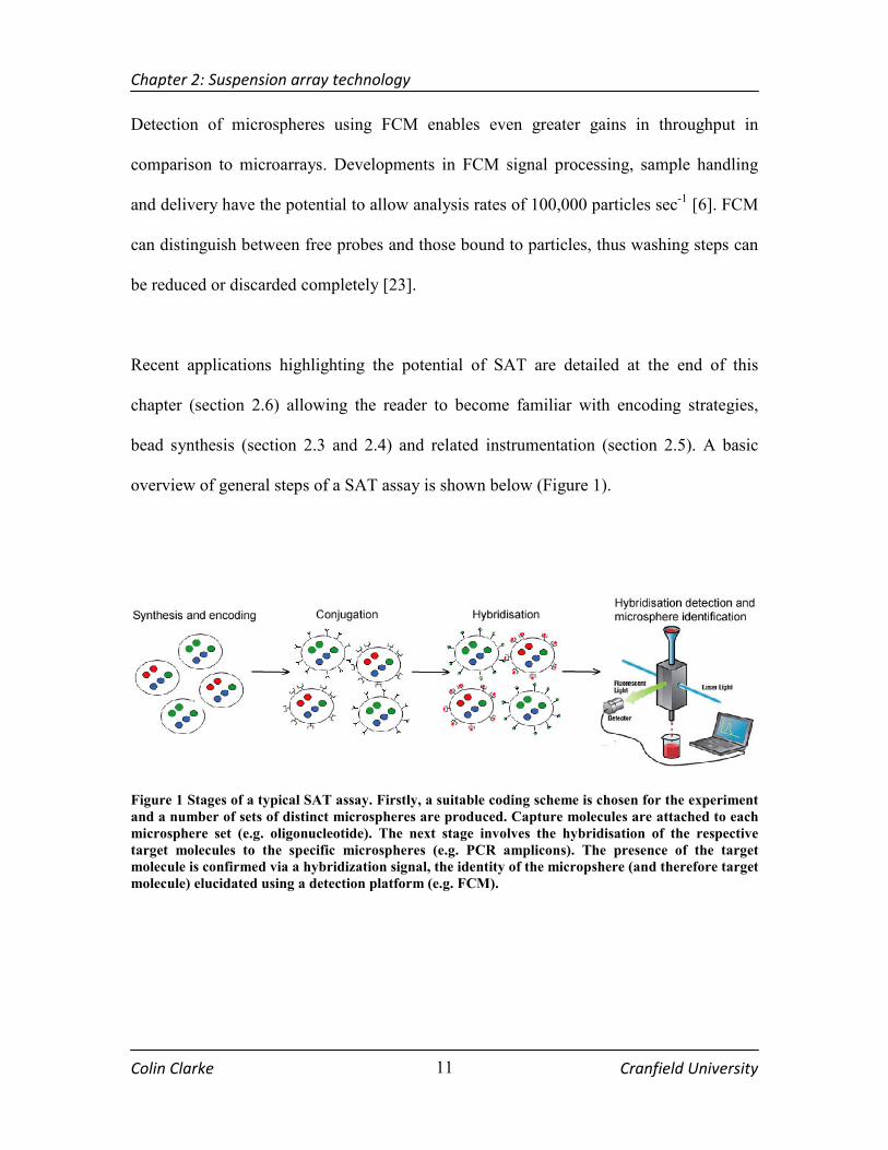
overview of general steps of a SAT assay is shown below (Figure 1).
Figure 1 Stages of a typical SAT assay. Firstly, a suitable coding scheme is chosen for the experiment
and a number of sets of distinct microspheres are produced. Capture molecules are attached to each
microsphere set (e.g. oligonucleotide). The next stage involves the hybridisation of the respective
target molecules to the specific microspheres (e.g. PCR amplicons). The presence of the target
molecule is confirmed via a hybridization signal, the identity of the micropshere (and therefore target
molecule) elucidated using a detection platform (e.g. FCM).

Chapter 2: Suspension array technology
Colin Clarke Cranfield University
12
2.3 Encoding schemes
There have been examples of various types of encoding schemes proposed for SAT but
by far the most popular is optical encoding. The likely reason for the success of
fluorescent encoded microspheres is the suitability for detection with flow cytometry
allowing high throughput detection (section 2.5.5 and chapter 3). Optical encoding theory
(section 2.3.1) and novel methods for encoding using nanocyrstal flourophores (section
2.3.2) are described. Non optical encoding schemes have also been proposed and are
outlined below (section 2.2.3).
2.3.1 Optical encoding
As stated above, the most popular encoding scheme described in the literature is optical
encoding via florescent dyes or nanocyrstals. Optically encoded SAT is achieved through
controlled internal combinatorial doping with various chromophores at discrete
concentrations (hence varying the intensity) for each microsphere and assigning a unique
spectral barcode. Decoding of the micropshere signal allows each microsphere target
molecule to be identified (Figure 2). Depending on the number of individual emission
wavelengths and intensity levels used the multiplex capacity of a particular encoding
approach can be calculated as follows:
1mC N −= (2.1)
Where: C = number of codes
N = number of intensity levels
m = the number of emission wavelengths
Chapter 2: Suspension array technology
Colin Clarke Cranfield University
13
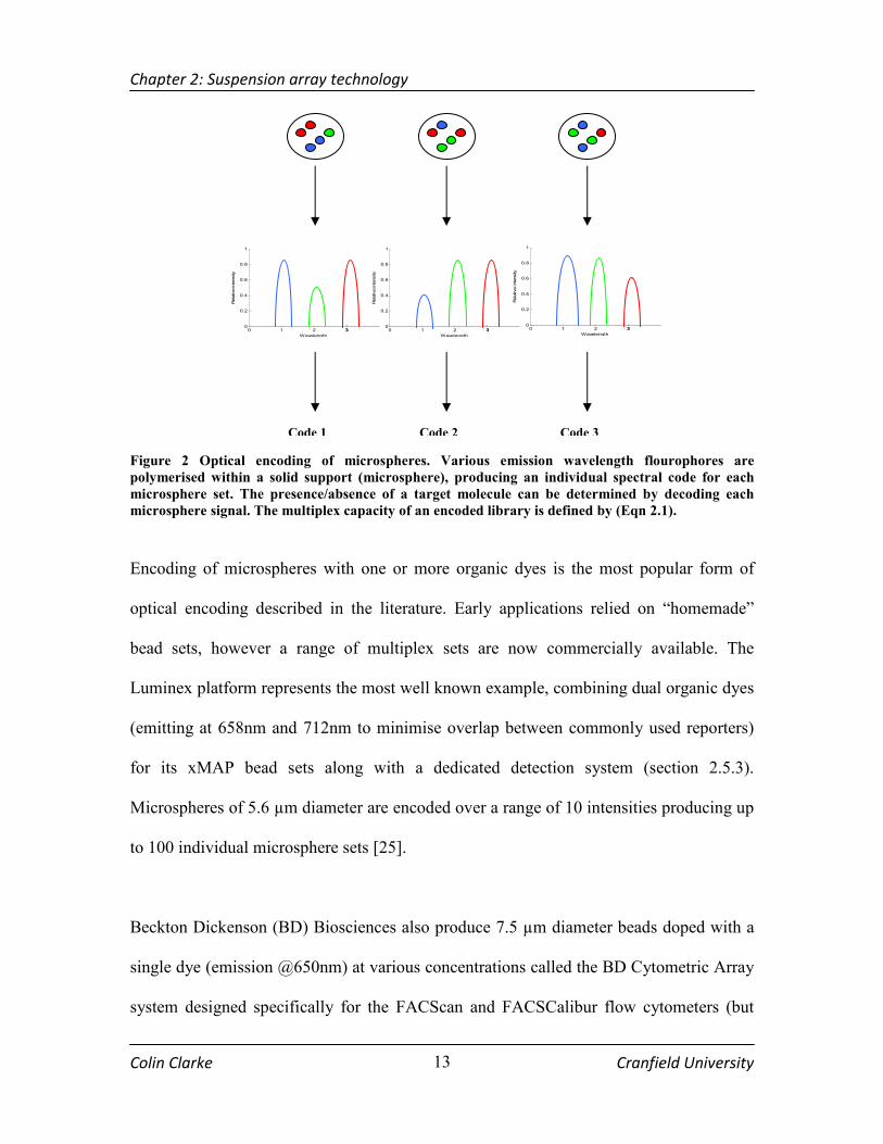
Figure 2 Optical encoding of microspheres. Various emission wavelength flourophores are
polymerised within a solid support (microsphere), producing an individual spectral code for each
microsphere set. The presence/absence of a target molecule can be determined by decoding each
microsphere signal. The multiplex capacity of an encoded library is defined by (Eqn 2.1).
Encoding of microspheres with one or more organic dyes is the most popular form of
optical encoding described in the literature. Early applications relied on “homemade”
bead sets, however a range of multiplex sets are now commercially available. The
Luminex platform represents the most well known example, combining dual organic dyes
(emitting at 658nm and 712nm to minimise overlap between commonly used reporters)
for its xMAP bead sets along with a dedicated detection system (section 2.5.3).
Microspheres of 5.6 µm diameter are encoded over a range of 10 intensities producing up
to 100 individual microsphere sets [25].
Beckton Dickenson (BD) Biosciences also produce 7.5 µm diameter beads doped with a
single dye (emission @650nm) at various concentrations called the BD Cytometric Array
system designed specifically for the FACScan and FACSCalibur flow cytometers (but
0 1 2 330
0.2
0.4
0.6
0.8
1
Wavelength
Relative intensity
0 1 2 330
0.2
0.4
0.6
0.8
1
Wavelength
Relative intensity
0 1 2 330
0.2
0.4
0.6
0.8
1
Wavelength
Relative intensity
Code 1 Code 2 Code 3
Chapter 2: Suspension array technology
Colin Clarke Cranfield University
14
also compatible with any cytometer with a 488nm laser) [26, 27]. Several other
companies manufacture a range of encoded microspheres including Spherotech, Duke
Scientific and Bang’s Laboratories. Organic dye based beads have been successful in a
range of applications including human immunodeficiency virus (HIV) analysis, thyroid
hormone analysis [28] and infectious disease monitoring (section 2.7)[29].
While organic dye based methods have proved useful in a range of applications, the level
of multiplexing has not reached the capacity required for post genomic technologies. The
narrow excitation wavelengths of organic dyes increase the complexity of
instrumentation; as more colours are added to the encoding scheme, additional excitation
sources are required prohibiting expansion [8].
2.3.2 Nanocyrstal encoding
Nanotechnology is concerned with the chemical and physical properties of materials with
dimensions in the order of magnitude of one billionth of a metre. Nanoscience applies a
new philosophy to manufacturing techniques implementing a bottom up approach,
starting with a single atom and adding atoms until the design is complete. Researchers are
rapidly developing nano-materials that will have a profound impact on all aspects of life
over the next decade, none more so than biology and medicine [30]. The first product of
the nanotechnology age with applications in the biological sciences is fluorescent
semiconductor nanocyrstals or quantum dots. QDs have been under investigation since
the 1970s, however their applicability to the life sciences had been limited until recent
novel advances in surface chemistry and synthesis methods [31, 32].

Chapter 2: Suspension array technology
Colin Clarke Cranfield University
15
QDs are composed of semiconductor materials such as Cd and Se, synthesis is precisely
controlled so that the QD dimensions are of the nanometre scale, typically 2-10nm [31].
When a semiconductor material such as CdSe exists at a size less than a critical quantum
measurement known as the exciton Bohr radius, the quantum confinement effect occurs
altering the electronic and optical properties in comparison to the bulk material. The
quantum confinement effect is due to the uncertainty relation that causes the energies of
an electron or hole to increase as the wave functions are confined to a smaller space [33].
Electrons are excited from the ground state to an excited state, when returning to the
ground state energy is released in the form of photons (fluorescence). The further the
electrons are from the ground state, the more energy is released and hence the further into
the UV region the QD will emit. The size, and/or composition of the QD is directly
proportional to the emission wavelength, so by varying the size or varying the synthesis
material of a single QD from the same material a range of different coloured dots can be
created [31]. The emission spectra of six sizes of CdSe QD are shown below, the
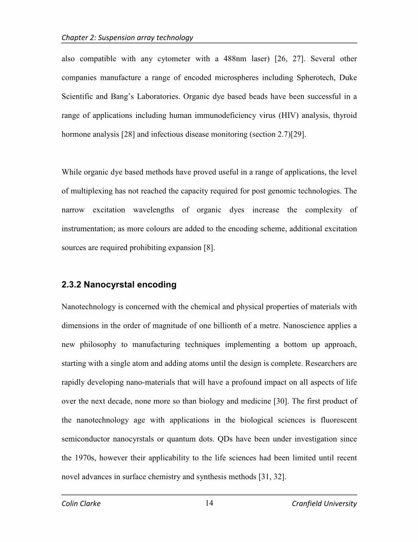
adsorption spectrum is also shown (Figure 3).
At present, organic dyes are the popular choice for fluorescence imaging and detection;
however organic dyes have a number of drawbacks including rapid photobleaching, red
tailing of peaks, narrow excitation spectra and broad emission spectra. QDs have been the
focus of intense research recently due to the inherent advantages of QDs over fluorescent
dyes, including size dependant emission wavelength, large excitation spectrum, narrow
Gaussian emission spectrum (full width half maximum (FWHM) = 20 – 40 nm) and an
extended photo-stable lifetime [31].
Chapter 2: Suspension array technology
Colin Clarke Cranfield University
16
Figure 3 Emission spectra of 6 different QDs. The absorption spectrum of the 510nm emitting QDs is
shown in black. Adapted from [34]. In terms of SAT the biggest advantage of QDs over organic dyes
is the relatively narrow emission spectrum (20 – 40 FWHM) and broad excitation spectrum which
allows excitation of multiple QDs with a single laser.
The current cost of QDs for encoding has been considered a limitation. QD synthesis
methods currently produce milligram batches requiring expensive chemicals. In Yu and
Peng’s synthesis method, 90% of the cost of QD production is attributed to the solvents
trioctylphosphine oxide (TOPO) or octadecene (ODE) in which the QDs are ‘grown’
[35]. Recent work by Asokan’s group demonstrated that the organic solvents could be
replaced by heat transfer (HT) fluids in the manufacture of CdSe QDs. The findings of
the study demonstrated HT fluids were viable alternatives, it was also demonstrated that
during the synthesis of smaller QDs the HT fluids were superior. The group concluded
that the cost of QD production could be decreased by ~80%, hence this advance should
accelerate uptake of QD technology within the community [36].
Chapter 2: Suspension array technology
Colin Clarke Cranfield University
17
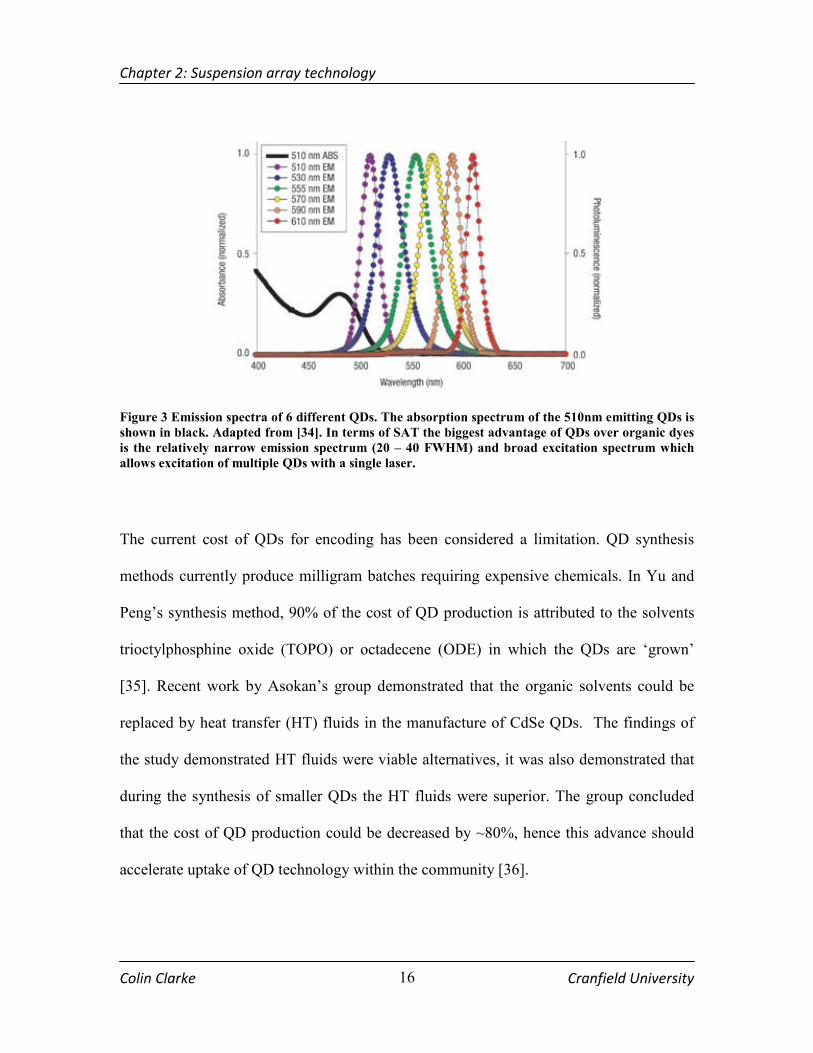
QDs have the potential to replace organic dyes for optically encoded SAT and QD
encoded microspheres are currently gaining popularity for such applications (Figure 4).
The broad excitation and relatively narrow emission spectrum of QDs require single laser
excitation, decreasing detection instrumentation complexity when additional colours are
added to the encoding scheme; furthermore there is reduced overlap between fluorescent
emission spectra. The photostability of QDs also allow more reproducible quantitative
results in comparison to organic dyes. These advantages significantly increase the
multiplex capacity beyond that of organic dyes. Considering Eqn 2.1 (page 12), the use of
QDs expand this capacity to that required for large scale genetic analysis, realistically 5-6
colours could be used and 10,000-40,000 unique codes may be produced [37] allowing
the multiplexing levels common with high density microarrays to be achieved.
Figure 4 Fluorescent micrograph of CdSe/ZnS QDEM. The microspheres are doped with QDs
emitting at 484nm,508nm,547nm,575nm and 611 nm [37].

Chapter 2: Suspension array technology
Colin Clarke Cranfield University
18
2.3.3 Non optical encoding schemes
As stated above, the resurgence of interest in SAT was primarily due to fluorescent
encoding strategies. While the focus of this work is on optical encoding, alternative
coding schemes have been previously demonstrated and are described here for
completeness.
Physical encoding relies on the measurement of physical characteristics of particles such
as size. The earliest examples of microspheres relied on decoding the scattering
properties of various sized microspheres [17]. Benecky et al. described the detection of
hepatitis B surface antigen using a multiplex bead library distinguishable by particle size
through the measurement of scattered light. Identification was possible when each
particular bead had 0.1 µm difference in bead size. The group used the sandwich assay
format and upon presence of the required antibodies aggregates formed, changing the
scatter signal [38]. Particle shape is also employed by 3D molecular sciences; however
this encoding scheme is not suitable for high multiplex levels but can be combined with
other encoding schemes to increase multiplex capacity.
Raman encoding of microspheres has previously been reported. Such methods rely on the
surface enhanced resonant Raman spectra (SERRS) effect to achieve the ultrasensitive
measurements required. When a molecule is in close proximity to a fractally rough
colloidal metal such as gold or silver and if the incident light is resonant with the
molecule and plasmon of the metal, the SERRS effect is observed. The encapsulation of
gold particles in silica has been shown to overcome problems with interference between

Chapter 2: Suspension array technology
Colin Clarke Cranfield University
19
the molecules and the metal, enhancing the signal by a factor of 1013 – 1014 [39]. Mirkin
et al. have shown the effectiveness of the technique to be suitable for multiplex analysis
of oligonucleotides [40]. The combination of infrared and Raman probes to encode
microspheres is also a possibility. Fenniri et al. created 24 unique coding signatures
through the polymerisation of styrene and alkyl styrene monomers suggesting further use
for combinatorial libraries [41]. Doering and Nie state that while these Raman and
infrared encoding can be used in a multiplex format they suggest the spectral decoding
may be limited [39], however recent work has shown that the discrimination of Raman
probes is possible using a modified flow cytometer and principal component analysis
(PCA) [42, 43].
Graphical encoding involves the classification of shapes; akin to supermarket barcodes.
The creation of microbarcodes has been achieved by fusing blocks containing rare earth
glasses (chosen due to narrow FWHM and large quantum efficiency) in a specific pattern
on glass ribbons. Each microbarcode could be distinguished using a UV lamp and optical
microscope or laser scanning cytometry (section 2.5.1). The authors hypothesised that up
to 1 million combinations are possible. To date this method has been demonstrated with
an assay to distinguish between human and microbial DNA [44]. Graphical encoding can
also be achieving using striped cylindrical metal nanorods or nanobarcodes, formed by
the deposition of gold and silver onto mesoporous aluminium films. 100 different strip
patterns were created that could be reasonably identified using an optical microscope.
Chemical modification of the surface for biofunctionality was also demonstrated [45].

Chapter 2: Suspension array technology
Colin Clarke Cranfield University
20
Electronic encoding of microspheres has also been reported. The first example employed
a semiconductor radio frequency (RF) device (analogous to radio frequency identification
tags (RFID)) enclosed in chemically inert layer. Each of the radio device containers was
assigned a unique frequency code and formed the building blocks of the microsphere
codes. Decoding of the micro-transponders was achieved using a custom built radio
frequency memory retrieval device. These types of codes offer high levels of
multiplexing. A major drawback cited is the large size of the microspheres, although
research is progressing toward the development of smaller RF devices. Miniature
electronic transmitters use an integrated circuit connected to a photovoltaic cell and
antenna. Each of the microspheres is decoded using capillary electrophoresis with laser
activated code transmission [46].
2.4 Microsphere synthesis, encoding and bio-conjugation
The production of optically encoded beads has three phases; the solid
support/microparticle must be manufactured, usually from polymers such as polystyrene,
Latex or methylacrylate. The microspheres must also be doped with the dye of choice
(organic or nanocyrstal), and the target specific capture molecule attached. Optically
encoded microsphere quality depends on a number of factors including the size range,
stability, uniformity and the ability to retain the fluorescent dye. It is also important to
minimise the surface texture in order to reduce light scatter. Recently there has been an
increased focus on the methodology required to create large quantities of microspheres
economically.

Chapter 2: Suspension array technology
Colin Clarke Cranfield University
21
The drop by drop method as its name suggests produces each micropshere sequentially. A
number of different variations of this method can be found in the literature such as the
injection of the polymeric solution through a needle, when the polymer leaves the needle
and enters the stabilising fluid flowing past the needle tip [47]. Yi et al. replaced the
needle with a capillary tube (Figure 5) [48], while Takeuchi et al. developed a
microfluidic device to control droplet formation [49].
Figure 5 The formation of monodisperse microspheres via drop by drop process [48]. Microspheres
are formed upon the ejection of droplets from the capillary tube aqueous phase to an oil based phase
where spontaneous formation of microspheres occurs. Variations of this process involve the
replacement of the capillary tube with a needle or microfluidic platform.
Microspheres can also be formed simultaneously, using solvent extraction/evaporation
principles. These techniques were found to be unpredictable in terms of particle size and
homogeneity of the populations. Moreover, simultaneous bead formation using this
method is unsuitable for producing large quantities of microspheres economically [50].
Laminar jet disintegration techniques again form microspheres simultaneously; the jet
breaks up into uniform droplets due to capillary instability or oscillatory stimulation.
These jet based techniques despite perfect size distribution are unable to produce
microspheres below 25µm. Martin-Banderas et al. overcame this limitation by

Chapter 2: Suspension array technology
Colin Clarke Cranfield University
22
application of a flow focussing technique to produce a microjet under controlled
conditions [51]. Monodisperse microparticles with excellent size accuracy (~5µm) were
produced. The group produced fluorescently encoded microspheres and suggested that
the high versatility of the technique could be applied to bead based arrays.
Figure 6 Scanning electron microscope(SEM) image of undoped microparticles produced by the flow
focussing method [51]. The surface texture of these microspheres is “golf ball like” which may
increase light scattering during detection.
The majority of methods encode the microspheres post synthesis, however it is worth
noting that attempts have been made at polymerising QDs directly into the microspheres
during synthesis [52]. To date this method has only been achieved using specially
designed polymers and QD-ligands, no biological applications have been reported. This
method suffers drawbacks from the tendency of colloidal QDs to aggregate within the
polymer. The most successful manufacturing methods employ a two stage process, firstly
the microsphere are synthesised and flourophores are subsequently added.
There are a number of methods for nanocyrstal encoding of microspheres. The deposition
of nanocyrstals onto labelled polystyrene beads has previously been described using the
so-called layer by layer method [53]. Polystyrene (PS) beads were used as the solid
support, and several layers of QDs were built up in the surface via electrostatic

Chapter 2: Suspension array technology
Colin Clarke Cranfield University
23
interactions. The number of monochromatic QD layers was precisely controlled to
encode the beads. Once the layer by layer deposition of QDs was complete successful
conjugation of anti-immunoglobulin G to the microspheres was achieved [54].
Riegler et al. has described a method for encoding involving the immobilization of
nanocyrstals within the microsphere interior by demixing two solvents (phase transfer
process). The method described involves dissolving the QDs in a beads soluble solvent
e.g. toluene, this solution is then added to an immiscible solvent e.g. water. Upon
addition of the QDs they are transferred to the polymer phase (a process termed
demixing) resulting in the nanocyrstals being incorporated throughout the microspheres
via strong hydrophobic interactions. The method is similar to the swelling method (see
below); however diffusion plays no part in the process. Using this approach fluorescence
was found to be stable, with no surface texture and microspheres were amenable to
bioconjugation [47].
Nanocyrstals may also be injected into porous microspheres as described by Nie et al.
[55]. Initial attempts swelled the microspheres and allowed QDs to diffuse into the
internal structure of the microsphere [37], it was noted however that QDs were only
absorbed at the surface of the microspheres and they tended to leach from the beads in
protein solution and buffer [56]. To overcome these limitations mesoporous polystyrene
beads were added to solutions containing precise ratios of various QDs with different
emission wavelengths, showing rapid absorption of QDs within the internal porous
structure and immobilisation of QDs through hydrophobic interactions. Beads prepared
Chapter 2: Suspension array technology
Colin Clarke Cranfield University
24
by this method showed no leakage of QDs when the process had been completed. FCM
measurements showed the beads to be 100 times brighter and a observed 5 fold increase
in encoding uniformity in comparison to non-porous microspheres. This method has
produced by far the best results to date for uniform encoding and signal strength. Cao et
al. suggested that these polystyrene beads may be stabilised by encapsulating each bead
with a layer of silica [57]. The deposition of silica does not effect the bead signal, and
increases the stability of the microsphere during the hybridisation step of an assay.
The most popular approach for bioconjugation is the attachment of specific nucleic acid
and protein molecules to carboxylated microspheres. Carboxyl groups on the microsphere
surface are activated using 1-eythl-3-(3-dimethylaminopropyl)-carbodiimide (EDC)
transforming the carboxyl groups to amine reactive sulfo-NHS esters. Conjugation
between the carboxyl groups and the amino modified nucleic acids (or protein primary
amides) takes place forming an amide bond. A spacer may also be included which in
some instances can increase the efficiency of hybridisation [9, 19, 57, 58].
2.5 Detection platforms
2.5.1 Laser scanning cytometry
Laser scanning cytometry (LSC), originally proposed to overcome the limitations of
FCM for surgical oncology [59-61], has been proposed as an alternative detection
platform for fluorescent microspheres [23]. This technique uses multiple lasers to scan
over the imaging surface without the same focusing constraints as fluorescence
microscopes. The technique is mostly used in SAT to decode graphical arrays however it
Chapter 2: Suspension array technology
Colin Clarke Cranfield University
25
has also been proposed as an alternative to flow cytometry for optical encoding. Coleman
et al. evaluated the possibility of combining optically encoded microspheres on a planar
surface. LSC based optically encoded microsphere measurement however, suffers from a
number of limitations. Firstly if the height of the imaging surface is not uniform some
microspheres were not in focus thus requiring multiple images to be acquired. Secondly,
the microspheres were prone to aggregation on the planar surface possibly due to
convection currents which may cause the microspheres to move and aggregate [62].
2.5.2 Microfluidic platforms
Microfluidic devices are capable of high throughput analysis by means of parallel assays,
multiplex capacity and automation. The utilisation of microspheres as solid supports with
microfluidics is an attractive option. The surface area to volume increase offered by the
microspheres improves the sensitivity of such assays due to the higher reaction
efficiency. Currently microfluidic platforms approaches are however limited in
comparison to FCM in terms of throughput and availability [54].
2.5.3 The Luminex system
The Luminex platform is a flow based system designed specifically for the analysis of
dual organic dye encoded microspheres. Luminex has evolved from the FlowMetrix
system described by Fulton and co-workers [18], FlowMetrix based microspheres were
originally produced as a set of 64 distinct microspheres for a standard cytometer (BD
FACScan). The system ran digital signal processing software for real-time analysis of the

Chapter 2: Suspension array technology
Colin Clarke Cranfield University
26
microspheres. The main disadvantage of the FlowMetrix microspheres was the
fluorescence overlap between the encoding dyes and reporter (hybridisation signal)
molecule and compensation was required [63].
Figure 7 (A) Luminex Flow System showing the dual laser configuration (YAG and red diode) [64].
Microspheres flow past the excitation point individually and spectral responses collected. (B) FL2
and FL3 values for 64 different types of microspheres from the FlowMetrix system. Average of 300
microspheres events per set used [18].
To this end the dedicated flow based bench top system, the Luminex 100, was designed
specifically for analysis of FlowMetrix microspheres. The Luminex system employs a
635nm red diode laser to excite the microspheres and a yttrium aluminium garnet (YAG)
532nm laser for improved reporter dye (R-phycoerythrin) excitation in comparison to a
488nm laser. Using this system 100 unique codes can be created. The Luminex platform
has been successfully applied in a range of assays including immunoassays [65-69],
cytokine analysis [70-75] and nucleic acid analysis [7, 76-82] amongst others.
(A) (B)
Chapter 2: Suspension array technology
Colin Clarke Cranfield University
27
2.5.4 The Mosaic system
The quantum dot corporation (QDC) one of the main suppliers of commercial QDs
developed the Mosaic system (the world’s first gene-expression system based on Qbead
(QDEM) technology) in collaboration with Matushita/Panasonic. The Mosaic gene
expression assay system provided a complete and optimized platform of instrumentation,
software and reagents for custom-multiplexed, high-content, and mid-throughput gene
expression analysis from cells or tissues. The system contains an inverted epifluorescence
microscope equipped with a 405nm laser and CCD detector; multiplex assays are carried
out in multiwell plates, using image recognition software to decode the QDEMs.
However CCDs suffer from low sensitivities compared to PMTs [23]. In 2006 the QDC
was acquired by Invitrogen and since the takeover the Mosaic system seems to have been
discontinued for reasons unknown.
2.5.5 Flow Cytometry
Flow cytometry is a well developed technology used for a wide range of analyses. FCM
equipment is also available in a large number of locations including hospitals,
universities and core laboratories and was the original detection platform for SAT
analysis. The detection of QDEMs with FCM offers the possibility of expanding basic
single laser FCM analyzer applicability (all QDs are excited by a single wavelength) to
genomic and proteomic applications. FCM provides a well developed detection platform
for high speed sensitive multiparameter measurements making it ideal for analysis of
optically encoded microspheres [83].
Chapter 2: Suspension array technology
Colin Clarke Cranfield University
28
In terms of throughput FCM is unmatched. Even basic bench top analysers are capable of
making highly sensitive measurements over four or more colours. Flow cytometry in
conjunction with sophisticated sample handling techniques can yield a sampling rate of
one 96-well plate/min. Using as little as 1µl sample volume, a 100plex assay can be
completed in less than a minute 1 min, which translates to 120 million data points per day
[6].
This thesis concentrates on the combination of fluorescent encoding of microspheres and
flow cytometry for high throughput genomic and proteomic assays. In chapter 3 FCM
instrumentation is examined in detail (section 3.3) and the analysis of multicolour
QDEMs with an 4 intensity/4 colour encoding scheme is described (section 3.4).
2.6 Applications
Bolstered by recent innovations, SAT is receiving increasing attention for high
throughput analysis of genes, proteins and a host of other biomolecular species [19]. The
following sections discuss examples of SAT applications in proteomics, SNP genotyping
and gene expression. These are by no means the only applications of SAT assays
however the following lists focuses on the applications which stand to gain the most
benefit from the increased multiplexing analysis offered by fluorescent encoding
QDEMs.

Chapter 2: Suspension array technology
Colin Clarke Cranfield University
29
2.6.1 SNP genotyping
SNPs are single base substitutions occurring within the general population at a frequency
of greater than 1% and accounting for ~80% of the genetic variance between individuals.
Located every ~1000 base pairs it is estimated that there are in excess of 3 million SNPs
located in the human genome [84]. Mutations, particularly single nucleotide
polymorphisms, are thought to play a role in an organisms response to drugs, bacteria,
disease, viruses and toxins [3, 85], the understanding of these roles will impact a number
of major areas.
SNPs are providing avenues for novel agricultural research to increase rice, wheat and
soya bean crop yield, decrease susceptibility to particular diseases and reduce the amount
of herbicide applied [86, 87]. Microorganism SNP profiles are also important as
demonstrated by recent outbreaks of E.coli as a result of mutations and the resistance of
HIV to treatment due to a high frequency of mutation[88].
The application of knowledge gained through SNP identification and relation to
phenotype for a population has the potential to revolutionise areas such as medicine and
drug discovery by moving away from the “one size fits all” philosophy to a more
personalised therapy based on interindividual genetic variations i.e. “the right drug for the
right patient” and it is this area known as pharmacogenomics which promises to yield the
greatest impact on human life.
Chapter 2: Suspension array technology
Colin Clarke Cranfield University
30
Pharmacogenomics aims to elucidate the genetic basis for disease susceptibility, variable
drug response (efficacy) and adverse drug reactions (toxicity) [89].To this end the SNP
Consortium (TSC) has been formed by the world leading pharmaceutical and academic
laboratories to discover and map hundreds and thousands of SNPs with a view to
identification of genes related to novel disease markers and drug targets leading to
individual drug therapies and diagnostic tests [90].
It is clear cost effective SNP genotyping platforms will be required to profile large
numbers of patients and control DNA samples to elucidate the information required in
order to draw associations for pharmacogenomic applications. Depending on the study
~5000 tests may be needed to identify functional candidates. When performing a genome
scan without prior functional evidence as many as 250,000 – 500,000 loci need to be
analysed. The nature of association studies requires multiple testing on the same patient
samples. It is estimated that 80% of all haplotypes occur in all populations with only 8%
being population specific. Research carried out for the European and Japanese
populations have demonstrated the need for 20% more SNPs to cover both populations
versus one, research is planned for the African population and the amount of SNPs
required to cover all three populations is expected to increase. Moreover the integration
of this technology with various other types of ‘omic’ data is critical in attaining
maximum benefit from SNP analysis in medicine and drug discovery [89].
The analysis of single nucleotide polymorphisms has included methods such as single
strand conformation polymorphism analysis (SSCP) [91-93], gel length restriction

Chapter 2: Suspension array technology
Colin Clarke Cranfield University
31
fragment length polymorphism [94, 95], allele specific oligonucleotide (ASO)
hybridisation [96], oligonucleotide ligation assay (OLA) [97] and allele specific primer
extension assays (ASPE) [98, 99]. In terms of detection and readout of alleles from the
methodologies above, a number of new technologies have been developed for
discrimination of signals based on hybridisation or enzymatic cleavage, including mass
spectrometry (MS), planar array based platforms [100-102] and SAT. Several studies
have reported the suitability of microsphere based assays for SNP genotyping citing rapid
data acquisition and excellent sensitivity. SNP assay formats have largely taken the route
of OLA or single base chain extension [25]. The first combination of SNP genotyping
and multiplexed microspheres was described in 1997 by Fulton et al. using 16 sequence
specific oligonucleotide probes and demonstrated the sensitivity, precision and speed of
the assay format [18].
More recently a number of groups have demonstrated the effectiveness of optically (both
organic dye and nanocyrstal) encoded microspheres as a detection platform for SNP
genotyping. Ye and co-workers utilised ASPE for a multiplexed SNP genotyping study,
with excellent correlation to that of sequencing. The authors also suggested that using a
flow cytometer up to 30,000 genotypes could be analysed every eight hours [103],
furthermore the group estimated that the cost per SNP is less than $0.20. Single base
chain extension has also been detected using fluorescent microspheres. The potential
throughput of the assay was estimated as 120,000 genotypes per day, however the cost
was slightly higher [104].
Chapter 2: Suspension array technology
Colin Clarke Cranfield University
32
Luminex xMAP technology has been used extensively for SNP genotyping; Armstrong et
al. developed and validated a 32-plex SNP genotyping assay for 8 different genes. Four
different ASOs were used for each mutation and employed to detect the allele where the
highest fluorescence for each of the four possible microspheres determined the genotype.
A direct comparison of results with the TaqMan assay was carried out. The results of the
39 genotypes were found to be in good correlation between both assays [58]. Numerous
other examples can be found in the literature for organic dye encoded microspheres used
for SNP genotyping including application for basal cell carcinoma [105] and cervical
cancer [106].
QDEMs have also been applied to SNP genotyping. The most significant work (and the
first to apply QD encoded microspheres to SNPs) to date was carried out by Mahoney et
al. As a proof of concept the P450 gene family was chosen for study, due to its
importance in drug metabolism and difficulty to genotype (due to the high degree of
homology between members). QD encoded microspheres were found to highly accurate
(100% concordant with DNA sequencing); furthermore the method also had a higher call
rate (although it was suggested that this may have been due to PCR amplicons not being
purified, suggesting that a PCR purification step maybe avoided when using
microspheres). Also noted was the decrease in the DNA concentration required for the
assay (1 ng Genomic DNA), substantially less than that required by other assays without
direct amplification of the genomic strand. The group also confirmed the advantages over
planar arrays stated above. Figure 8 below shows the methodology used [9].

Chapter 2: Suspension array technology
Colin Clarke Cranfield University
33
Figure 8 SNP system employed by Xu et al. PCR of the genomic DNA is carried out at various SNP
loci, biotin labelled amplicons are hybridised to allele specific QD encoded microspheres with unique
spectra. The presence of bound target is determined by presence of the reporter signal, streptavidin-
PE-CY5. Microspheres are identified using FCM [9].

Chapter 2: Suspension array technology
Colin Clarke Cranfield University
34
2.6.2 Gene-expression
To date several reports have detailed gene expression studies using SAT. Fuja et al.
determined the expression levels of four transcripts, BRCA1, MGB1, DLG1 and ACT1
using SAT. Organic dye based microspheres were conjugated to transcript specific probes
by covalent coupling. The results from the study were compared to quantitative real-time
polymerase chain reaction (RT-PCR). The authors concluded that the results were
concordant with RT-PCR [20] and multiplexed bead assays are a viable alternative to
planar arrays for gene-expression profiling. In 2001, the beadsArray™ for the detection
of gene expression (BADGE) was carried out on the Luminex platform; a decrease in
hybridisation time over other assays was noted. The method also out performed
quantitative RT-PCR in terms of multiplexing ability and the amount of RNA required
[107].
Increasing the multiplexing levels of gene-expression profiling using SAT is crucial and
to this end attention turned to QDEMs. The Mosaic Q1000 system was designed
specifically for mid throughput gene expression analysis. In a recent study Eastman et al.
used 8µm magnetic microspheres for convenience in sample preparation, liquid handling
and reduction of the background signal. Specific nucleotides were attached to QDEMs
were used to screen ~100 genes (455 are possible with the coding scheme used).
Biotinylated cDNA was produced from RNA and hybridised to the microspheres,
streptavidin coupled to an infrared emitting QD for hybridisation. The results of the study
showed a high agreement with GeneChip microarrays and improved on results aqquired
by the Luminex platform [108].

Chapter 2: Suspension array technology
Colin Clarke Cranfield University
35
2.6.3 Proteomics
Quantitative proteomics has been suggested as one area where multiplex microsphere
libraries may be used to determine the amount and state of proteins in a sample. In
comparison to ELISA based techniques which are carried out in microwell plates,
microspheres act as the solid support for capture antibodies. The sensitivity of ELISA
based assays is in the pg/ml range using high affinity monoclonal antibodies and is easily
automated [19]. The large sample sizes required for microplate based methods, led to the
application of microarray-type techniques. Capture antibodies are spotted onto glass
membranes and glass slides. In terms of protein concentration the best results have been
observed using the sandwich assay design. The reproducibility and reliability of
microarray based ELISA has not reached the clinical level thus far however and [109]
bead based multiplexing assays have been shown to be a viable alternative to slide based
methods for highly parallel analysis.
The earliest examples of microsphere based sandwich assays (Figure 9 B) concentrated
on the detection of multiple cytokines using the FlowMetrix system. Using this method
Carson et al. reported that the FlowMetrix assay overcame significant variation from
experiment to experiment and also plate to plate variation observed with ELISA assays
[110].

Chapter 2: Suspension array technology
Colin Clarke Cranfield University
36
Figure 9 Example of protein SAT assay chemistry and detection. (A) Antigen conjugation for
analysis of blood and plasma antibodies. (B) Sandwich assay design. Adapted from[25].
Alternatively the antigen can be conjugated to the beads for the analysis of antibodies in
blood and plasma (Figure 9 A). For this assay the antigen is immobilised onto the
microsphere and a labelled class or isotope specific antibody is used to report the
presence of the analyte [19]. Applications include cryptosporidium antibodies in serum
and oral fluids [111] showing good correlation when compared with an equivalent ELISA
assay. McHugh et al. also applied the technique to the detection of antibodies to
cytomegalovirus and herpes simplex virus [112].
Encoded microspheres have also been applied to the study of carbohydrate-protein
interactions. An optically encoded microsphere is conjugated to a unique carbohydrate;
the microspheres are then incubated on a randomly ordered fibre optic array. The assay
allowed for the simultaneous measurement of carbohydrate binding proteins [113].
(A) (B)
Chapter 2: Suspension array technology
Colin Clarke Cranfield University
37
2.7 Thesis aims and objectives
It is clear that SAT has a great deal of potential in the analysis of genes and proteins for
post genomic applications. In order to perform the applications described in the previous
sections, particularly SNP genotyping and gene expression analysis at microarray
throughput levels an alternative to organic dyes must be found. QDs are an excellent
candidate for this role, due to single wavelength excitation and relatively narrower
emission peaks. The inherent advantages of QDs over organic dyes allow the
multiplexing capabilities of such assays to be extended. Current manufacturing processes
have progressed sufficiently enabling the production of bright, stable and reproducible
optically encoded microspheres.
FCM was chosen as the detection platform for QDEMs allowing sensitive measurements
of multiple fluorescence channels in high throughput. These fluorescent nanocyrstals are
naturally extendable to basic FCM bench top systems however the process of decoding
highly multiplexed SAT libraries may not be straightforward on current FCM equipment.
As the number of unique microspheres increases and additional emission wavelengths are
added to the coding scheme the classification of individual microspheres becomes more
difficult as the number of fluorescent parameters to consider increases.
Chapter 2: Suspension array technology
Colin Clarke Cranfield University
38
This work aims to investigate a number of classification schemes for the identification of
QDEMs from FCM data. A commonly used method, MPG is evaluated in chapter 3
followed by the development of supervised learning models. Support vector machines
(chapter 4) and artificial neural networks (chapter 5) were selected due to their suitability
for multiparameter data, high generalisation ability and previous success in the field
(section 4.2.3 and section 5.2.2). The accessibility of these techniques to the community
is also of considerable importance as such algorithms are not included at present with
FCM software.
The main objectives of this thesis are:
• To determine the optimum classification method for microsphere identification
for a QDEM FCM dataset obtained using a flow cytometer representative of those
found in research laboratories and the clinic.
• The following techniques were optimised for the data and the most suitable
methodology chosen:
o Multiparameter gating
o Support vector machines
o Artificial neural networks
• To develop a user friendly interface to carry out the most suitable method while
also providing common FCM software functionality (chapter 6), for the benefit of
lab based researchers.

Chapter 3: Flow cytometric analysis of nanocyrstal
encoded microspheres.
Chapter 3: Flow cytometric analysis of nanocyrstal encoded microspheres.
Colin Clarke Cranfield University 40
3.1 Overview
The focus of this chapter is to illustrate flow cytometer instrumentation, describe the
acquisition of the datasets used throughout this thesis and to evaluate current encoded
micropshere identification methods. The chapter is split into two distinct sections
beginning with a brief introduction to general flow cytometry (section 3.2), FCM
instrumentation and data processing (section 3.3). The second part of this chapter
describes the flow cytometric analysis of a nanocrystal encoded library (section 3.4) and
evaluation of a standard classification method - multiparameter gating - for the
identification of QDEMs (section 3.4).
3.2 Introduction
Cytometry is loosely defined as measurement of the physical and chemical characteristics
of cells. Flow cytometry is the process of measuring these characteristics for a fluid
stream of cells or particles (the analyte) flowing through an instrument called a flow
cytometer [114]. A flow cytometer enables multiple simultaneous measurements of light
scatter and fluorescence at the individual analyte level at very rapid rates. Flow
cytometers are subdivided into two categories, analysers and sorters; an analyser
measures the properties of each of the cells in the stream, an optional sorting module may
be present allowing separation of cells post analysis. (Sorters are not considered here, for
further information see [114, 115]).

Chapter 3: Flow cytometric analysis of nanocyrstal encoded microspheres.
Colin Clarke Cranfield University 41
During measurement a laser beam is passed through a fluid stream containing the
population of interest. Excitation of the analyte within the stream (sample core) results in
a signal dependant on the properties of the analyte in question. The physical properties of
a given analyte can be determined by measuring scattered light of two types. Side scatter
(SSC), detected at ~90° to the incident light is proportional to cell granularity and the
complexity of a cells internal structure (widely used in the differentiation of cells such as
granulocytes). Forward scatter (FSC), is a measurement of diffracted light, measured via
a photodiode at a small angle to the axis of the laser beam. Scattering is routinely used as
a ‘trigger’ for cell sorting. Excluding clinical haematology, all FCM analysis employs the
use of flourophores. The determination of non-physical characteristics of a cell may be
elucidated through labelling with an organic flourophore (e.g. fluoroscein isothiocyanate
(FITC)) attached to a carefully chosen primary or secondary antibody. In FCM
experiments data is generally presented as histograms or bivariate histograms either as
scatter, density or contour plots (see below).
FCM is a well established analysis platform and has applications in a broad range of
standard clinical diagnosis and research areas, ranging from DNA histogram analysis to
determine ploidy (number of chromosomes in a cell), DNA index S-phase fractions for
cancer diagnostics, immuno-phenotyping and of course SAT [116-120].

Chapter 3: Flow cytometric analysis of nanocyrstal encoded microspheres.
Colin Clarke Cranfield University 42
3.3 Flow cytometer instrumentation
3.3.1 Fluidics system
The flow cytometer fluidics system orders the sample into a stream and transports it
through the centre of the excitation or “observation” point. There are two types of fluidic
design implemented in modern flow cytometers, the flow cell and stream-in-air. Bench-
top cytometers such as the Beckman Coulter EPICS XL use the flow chamber or cell
design (Figure 10). All benchtop cytometers employ the flow cell design and are used in
conjunction with a laser (or mercury arc lamp source) (section 3.3.2). For an excellent
discussion of flow chamber design and stream-in-air flow systems see [121].
Figure 10 Flow cytometer flow cell, the sample is aspirated from the tube into the fluid stream where
it is hydrodynamically focussed to the centre (core). The greater the sheath pressure the more cells
pass though the laser at any given time. For micropshere analysis, the sheath fluid pressure is kept
low in order to allow each bead to pass through individually [121].
Within the flow cell the sample is injected into a rapidly flowing fluid (sheath fluid).
Principles of laminar flow keep the sample core separate from the sheath fluid by

Chapter 3: Flow cytometric analysis of nanocyrstal encoded microspheres.
Colin Clarke Cranfield University 43
accelerating the particles and restricting them to the centre of the core in a process known
as hydrodynamic focusing. The pressure of the sheath and sample fluids is critical;
sample pressure must always be greater than the sheath fluid pressure. A pressure
regulator controls the sample flow rate by changing the sample pressure relative to the
sheath pressure. An increase in the sample pressure increases the flow rate by increasing
the width of the sample core allowing more analytes into the stream. However this may
lead to more than one cell passing through the excitation point at any given time.
Applications which use a high flow rate during analysis are generally used for qualitative
analysis for instance immunophenotyping where ultra-high throughput is desired [122].
Lower flow rates are used for analysis requiring more precise measurements analysis e.g.
DNA analysis [123] and SAT applications where a low flow rate is maintained to allow
measurement of single microsphere events. During operation the fluidic system must be
kept clear of debris and air bubbles to ensure the sample correctly intercepts the laser
beam. As the sample core is hydrodynamically focussed toward the centre of the fluidic
stream, the position of the sample within the core is a potential a source of excitation
intensity variation [121].
3.3.2 Excitation
Sample excitation is primarily achieved with a laser consisting of a cylindrical plasma
tube filled with an inert gas such as argon. The primary beam of bench top flow
cytometer is at 488nm, although some flow cytometers carry a secondary source usually
either a red diode laser at 635nm or a UV mercury arc lamp at 375nm. The wavelength of
the laser is monitored and kept constant by means of feedback circuitry. The alignment of

Chapter 3: Flow cytometric analysis of nanocyrstal encoded microspheres.
Colin Clarke Cranfield University 44
the laser is critical in FCM and must remain focussed on the sample core, in bench-top
flow cytometers no adjustment is necessary as the laser is pre-aligned and fixed in
position. The beam is directed through a spherical lens which causes the beam shape to
become elliptical, before finally entering a focussing lens allowing the beam to intercept
the sample core.
Advances in laser technology have produced very stable lasers for flow cytometry in
terms of output. Under light stabilized operation modes the laser can maintain an output
within ± 0.5% during continuous extended operation. Arc-lamp excitation sources usually
have an electronic feed back loop to correct for any instability. For the majority of the
arc-lamp lifetime the lamp may maintain ± 0.5% stability however toward the end of its
lifetime a larger variation in the intensity of the lamp is often observed [121].
3.3.3 Optics and detection
When a cell is passed through the laser excitation point the emitted side scatter (SSC) and
fluorescence signals are routed to the detectors via a system of beam splitters and optical
filters. Dichroic mirrors and lenses are used to direct light of a selected wavelength to a
particular detector. For example a 560 shortpass (SP) dichroic mirror transmits light of
less than or equal to 560nm, longer wavelengths are reflected at 45° from the angle of
incidence[121]. In the case of the Epics XL dichroic lenses are used for this purpose,
dichroic lenses are used to reflect light shorter than a specified wavelength (Figure 12).
Photomultiplier tube (PMT) and photodiode (PD) detectors are the detectors of choice for
FCM due to their high sensitivity. Optimisation of the detector for a particular
fluorescence signal is achieved through the use of bandpass (BP) filters allowing only a

Chapter 3: Flow cytometric analysis of nanocyrstal encoded microspheres.
Colin Clarke Cranfield University 45
narrow range of wavelengths to reach the detector (Figure 11). Other filters which may
be used with the flow cytometer are short-pass (SP) filters which transmit wavelengths of
light equal to or shorter than the required wavelength. Long-pass (LP) filters allow light
equal to or longer than the specified wavelength through.
Figure 11 Examples of the filter and mirror that form the optical bench. The optical bench route SSC
and fluorescent signals to the PMTs and PDs during FCM.
Optical filters may also contribute to fluorescence, especially those made from glass.
Large amounts of light from the excitation source scattered toward the collection optics
can induce fluorescence from these filters, interfering with analyte measurements [124].
The performance of the filter system in a flow cytometer is a probability based function
and hence there is always a possibility that an excitation photon may enter the detector
and be mistaken for sample fluorescence. Careful design of the filter combination is
required to minimize this potential source of variation. For example in a high efficiency
light collection system, an extra dichroic mirror can be used to decrease the possibility of
a 488nm photon entering the detector [125].

Chapter 3: Flow cytometric analysis of nanocyrstal encoded microspheres.
Colin Clarke Cranfield University 46
Figure 12 The EPICS XL optical bench FCM configuration was used for all measurements taken
during this thesis. Fluorescence is detected at 525nm, 575nm, 620nm and 675nm. Adapted from
[126].
The orientation at which the excitation and light collection optics within a flow cytometer
are held is termed the optical bench (Figure 12). Good design of the optical bench is
essential to optimise the total amount of light striking the detector. The linear range of the
optics is also important as there exists a dark current which will restrict the range and
must be limited through bench design. The high throughput nature of flow cytometry
means that each analyte is excited by the laser for a few microseconds, to obtain accurate
results the maximum amount of light must be captured. Modern flow cytometers have a
light collection efficiency of between 15%-25%, much improved in comparison to older
instruments [125]. Good light collection efficiency may also lead to an increase not only
in fluorescent light but also background and scattered light. It is desirable to reduce this
background noise to a minimum and also to ensure that the increase in fluorescence does
not saturate the detector, producing a non-linear response [125].

Chapter 3: Flow cytometric analysis of nanocyrstal encoded microspheres.
Colin Clarke Cranfield University 47
3.3.4 Electronics
Once light from an analyte is routed to the detector photons are converted to
photoelectrons, creating an electrical current. The amount of photons generated by
fluorescence emission is small and PMT dynodes amplify the signal through a number of
internal gain stages, known as preamplifier gain (PDs generally have no gain and are
therefore used for bright FSC measurements). The aim of the FCM electronics system
attempts to maximise the signal to noise ratio i.e. only the photons resulting from the
interaction of the sample and laser beam are collected. The PMT gain has been described
as “the least noisy gain available” in the flow cytometer; therefore adjustment of the PMT
voltages is generally preferable over amplifier gain.
Conversion of the detector output current to voltage is achieved using a transimpedance
amplifier producing a linear amplification of the signal. Following the restoration of the
signal baseline (removal of stray light and dark current), a further programmable
amplification stage allows measurements to be controlled by the operator for online
histogram adjustment. In order to filter the non-sample signals a discrimination parameter
is selected and a user defined threshold is applied. For example during DNA content
analysis the discriminator is defined on the DNA parameter e.g. propidium iodide
fluorescence, as the analysis measurement of non-nucleated cells is generally of little
interest. Only when the signal exceeds this discriminator threshold is the sample event
recorded. Following these operations a voltage pulse is produced, the height and area
(integral) of the pulses produced are measured. Integration of the pulse width is carried
out to account for large analytes in the flow cytometer (i.e. particles that are larger than

Chapter 3: Flow cytometric analysis of nanocyrstal encoded microspheres.
Colin Clarke Cranfield University 48
the laser beam width). Digitisation of the data is then carried out for conversion of
analogue voltages to numeric values using an analogue to digital converter and stored in a
flow cytometry standard (FCS) file (section 3.4.2).
Figure 13 FCM electronics overview. The schematic shows the general FCM signal processing stages
from when light enters the PMT detector until the sample measurements are written to FCS files.
*PMT detectors also include an internal gain stage.
The final part of signal processing is carried out on a PC for operations such as
compensation (user specified correction for overspill between detectors with a correction
matrix), linear to logarithmic amplification (conversion of linear signals to log signals for
data display is achieved using a log look-up table with the EPICS XL instrument) and
data analysis/display (section 3.4.1) can be performed [127]. The sophisticated
electronics of modern flow cytometers is unlikely to give rise to significant variation in
results [125].

Chapter 3: Flow cytometric analysis of nanocyrstal encoded microspheres.
Colin Clarke Cranfield University 49
3.3.5 The FCS filetype
The FCS 1.0 format was developed by the Society for Analytical Cytology in 1984,
necessitated by the need for a standard file format to allow FCM data acquired on one
computer to be used with other types of computer systems. The FCS 1.0 format consisted
of a four section file that formed the backbone for subsequent file formats (FCS 2.0 &
FCS 3.0). The first section of an FCS file is always the HEADER segment and designates
the FSC version of the file. The HEADER segment also contains the 8 byte offset values
that defines the remaining file sections. The TEXT segment contains the experimental
information including the instrument type, detector ids and acquisition time in the form of
keyword value pairs. An example of a common keyword value pair in a FCS file is
“$TOT/10000/”, the keyword is $TOT and the value is 10,000 – this specifies that a total
of 10,000 events were recorded.
The raw data from flow cytometry is stored in the DATA portion in one of four formats,
binary, floating point, double precision floating point and ASCII, defined by the
$DATATYPE keyword in the TEXT segment. The most common method of data storage
is binary integers corresponding to the scatter and fluorescent measurements in columns
and events stored in the order at which the analyte passes the laser beam known as a
listmode file. In flow cytometry each measurement of an analyte is termed an “event”,
with the cytometer outputting a 1 × p vector for p parameters (variables) when each
QDEM is excited. A dataset is a collection of events from any given analysis, in our case
a single QDEM population or a multiplexed solution of QDEMs. The ANALYSIS
section is an optional post analysis portion containing the results of data processing and
analysis with variables in keyword value format similar to the TEXT section [128, 129].

Chapter 3: Flow cytometric analysis of nanocyrstal encoded microspheres.
Colin Clarke Cranfield University 50
3.4 Application of a supervised FCM data analysis method for
QDEM classification.
This section discusses the suitability of a readily available method for subpopulation
classification for the identification of QDEMs from a commercially available library. The
acquisition of QDEM data using FCM and the application of MPG are outlined (section
3.4.1 and section 3.4.2). Finally the performance of MPG for QDEM identification is
discussed (section 3.4.3).
3.4.1 Multiparameter gating.
The majority of current FCM analysis is dependant on operator interpretation of results
from one dimensional histograms or two dimensional scatter plots [121]. These data
display methods are routinely used throughout FCM experiments from instrument setup
and acquisition to publication [130]. The simplest type of data display for flow cytometry
measurements are single parameter frequency histograms (intensity versus the numbers
of events), which is used routinely in cell cycle analysis. A logarithmic x-axis over a four
to five decade log scale allows populations with 10,000 to 100,000 fold differences in
intensity to be displayed, e.g. immunophenotype analysis where a high dynamic range is
observed. Linear scales are generally used for plotting FSC and SSC measurements.
Bivariate histograms or two dimensional scatter plots are also commonly used to
visualise FCM results (three dimensional plots are also possible but seldom used due to
the danger of misinterpretation). The relative intensities of the two selected fluorescence
and/or scatter parameters specify the x and y coordinates of the point on a plot - here both

Chapter 3: Flow cytometric analysis of nanocyrstal encoded microspheres.
Colin Clarke Cranfield University 51
the axes are logarithmically scaled. A limitation of the standard dot plot is that no
information is provided as to the proportion of events lying in each subpopulation. An
extension of the dot plot allows projection of the density of the subpopulations on the plot
to highlight regions based on the concentration of events. Alternatively a contour plot can
be produced where lines represent the density based elevation of points. An example of a
dual parameter QDEM plot can be seen below (Figure 14) the dots are shaded in relation
to the number of events present at each x y position.
In flow cytometry the definition of a region around a cluster observed on a bivariate
histogram of two parameters is termed a gate. Gating is essentially human supervised
classification method (expert method) of subpopulation identification in FCM in that the
user relies on prior knowledge of the system under measurement to define the regions on
a 1D or 2D scatter plot. The definition of a subpopulation across multiple fluorescence
detectors is known as multiparameter gating. MPG functionality is available in the
majority of FCM software. The process of MPG begins with a series of bivariate
histograms; the operator interprets these plots to manually define or “draw” the
classification boundaries. In future analyses the gates are applied to unknown samples,
events falling within a particular gate are classified with the designated label. The
classification of fluorescently encoded beads has previously been achieved using MPG,
although the libraries described were less complex than the QDEMs used in this study
[131-133]. Each micropshere was analysed individually and a gate defined on each
bivariate plot for the population, the process continued until all encoded microsphere
regions had been defined.

Chapter 3: Flow cytometric analysis of nanocyrstal encoded microspheres.
Colin Clarke Cranfield University 52
In the work that follows the MPG method is employed for the recognition of a QDEM
library with 20 individually encoded microsphere sets. The coding scheme employs 4 QD
colours emitting at 525nm, 575nm, 620nm and 675nm. The concentration was varied
over three intensity levels. Each class of microsphere was analysed individually on a
standard single laser flow cytometer at 488nm and 1000 events acquired for each type of
QDEM. Gates are combined on multiple parameters for each population individually by a
flow cytometer operator. Once the gates are defined for each microsphere unknown
solutions can be presented and the QDEMs present predicited. A set of microsphere
mixtures containing randomly selected QDEMs were prepared to act as an external
validation for each of classification methods. Current FCM software does not allow
internal testing of gating accuracy as the method relies heavily on user interpretation.
Figure 14 2D gating of nanocrystal microspheres. The complexity of the gating procedure is
increased for each colour in the encoding scheme. The microsphere can be classified by their position
on the bivariate histogram i.e. class 1 = R1 and class 2 = R2. Adapted from [133].
Note: An unsupervised clustering algorithm available in the Flojo FCM software suite
was also evaluated. However all analyses using this software were unsuccessful in that
the identity of clusters could not be established and the number of events per cluster were
imbalanced. The details of this study can be seen in appendix 1.

Chapter 3: Flow cytometric analysis of nanocyrstal encoded microspheres.
Colin Clarke Cranfield University 53
3.4.2 Materials and methods
A library of 20 carboxyl functionalised 5µM mesoporous methacrylate microspheres
(Table 2) containing composition tuneable QDs (Cyrstalplex, Pittsburgh, USA) was
analysed using FCM. For more information on QDEM specifications see appendix 3.
Table 2 Specification of each of the 20 QDEM used in this study. The relative intensity of each
micropshere is shown at each of the four possible wavelengths.
QD -Emission Wavelength QDEM
Code 525nm 575nm 620nm 675nm
QD0000 0 0 0 0
QD0001 0 0 0 1
QD0003 0 0 0 3
QD0010 0 0 1 0
QD0011 0 0 1 1
QD0100 0 1 0 0
QD0101 0 1 0 1
QD0110 0 1 1 0
QD0111 0 1 1 1
QD0202 0 2 0 2
QD1000 1 0 0 0
QD1001 1 0 0 1
QD1010 1 0 1 0
QD1011 1 0 1 1
QD1100 1 1 0 0
QD1101 1 1 0 1
QD1110 1 1 1 0
QD1111 1 1 1 1
QD2100 2 1 0 0
QD2200 2 2 0 0
All data used in this study was acquired in the laboratory by Clair Gallagher. FCM was
preformed using an EPICS XL (Beckman Coulter, FL, USA). The instrument was
equipped with a 488nm air-cooled argon laser and the standard four colour filter set-up
(525BP; 575BP; 625BP; 675BP). The EPICS XL uses digital signal processing (DSP)
electronics negating log amplifiers for logarithmic amplification of signals, conversion of
linear to log is achieved using a log look-up table. Fluorescence compensation
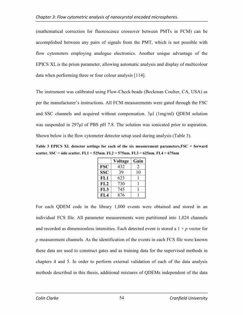
Chapter 3: Flow cytometric analysis of nanocyrstal encoded microspheres.
Colin Clarke Cranfield University 54
(mathematical correction for fluorescence crossover between PMTs in FCM) can be
accomplished between any pairs of signals from the PMT, which is not possible with
flow cytometers employing analogue electronics. Another unique advantage of the
EPICS XL is the prism parameter, allowing automatic analysis and display of multicolour
data when performing three or four colour analysis [114].
The instrument was calibrated using Flow-Check beads (Beckman Coulter, CA, USA) as
per the manufacturer’s instructions. All FCM measurements were gated through the FSC
and SSC channels and acquired without compensation. 3µl (1mg/ml) QDEM solution
was suspended in 297µl of PBS pH 7.8. The solution was sonicated prior to aspiration.
Shown below is the flow cytometer detector setup used during analysis (Table 3).
Table 3 EPICS XL detector settings for each of the six measurement parameters.FSC = forward
scatter. SSC = side scatter. FL1 = 525nm. FL2 = 575nm. FL3 = 625nm. FL4 = 675nm
Voltage Gain
FSC 432 2
SSC 39 10
FL1 623 1
FL2 730 1
FL3 745 1
FL4 876 1
For each QDEM code in the library 1,000 events were obtained and stored in an
individual FCS file. All parameter measurements were partitioned into 1,024 channels
and recorded as dimensionless intensities. Each detected event is stored a 1 × p vector for
p measurement channels. As the identification of the events in each FCS file were known
these data are used to construct gates and as training data for the supervised methods in
chapters 4 and 5. In order to perform external validation of each of the data analysis
methods described in this thesis, additional mixtures of QDEMs independent of the data

Chapter 3: Flow cytometric analysis of nanocyrstal encoded microspheres.
Colin Clarke Cranfield University 55
used for classifier construction were analysed (Table 4). All MPG was carried out using
FCS Express from De Novo software (http://www.denovosoftware.com/).
Table 4 Composition of the multiplexed solutions (QDEMs included are shown). In total there were
10 tests with various QDEM mixtures (chosen at random). This dataset was used as an external
validation of the classification methods described throughout the thesis. 500 events per QDEM in
solution were recorded.
Mixture #
1 2 3 4 5 6 7 8 9 10
QD0000 - - - - ���� - - ���� ���� -
QD0001 - - - - ���� ���� - ���� ���� ����
QD0003 - - ���� ���� - - ���� - - -
QD0010 - - - - - - ���� - - ����
QD0011 ���� - - - - ���� - ���� ���� ����
QD0100 - ���� - - ���� - - ���� - ����
QD0101 - - - - ���� - ���� ���� ���� ����
QD0110 ���� - - ���� ���� - - ���� ���� ����
QD0111 - - - - ���� - ���� ���� ���� ����
QD0202 - - ���� ���� - - - - - -
QD1000 - - - - - ���� ���� ���� - ����
QD1001 - - - - - - - - ���� ����
QD1010 - ���� - - - ���� - - - ����
QD1011 - ���� - ���� - ���� - ���� ���� ����
QD1100 ���� ���� - - - ���� - - ���� ����
QD1101 - - - ���� ���� ���� ���� ���� ���� ����
QD1110 ���� - - - ���� ���� ���� ���� ���� ����
QD1111 - - - ���� - - ���� ���� ���� ����
QD2100 - - ���� - - - ���� - - -
QD
EM
co
de
QD2200 - - ���� - - - ���� - - -
#Codes 4 4 4 6 8 8 10 12 12 15
Using the external validation set described above requires the determination of the
number of misclassifications and allows direct comparison between all classification
methods to be drawn. The number of misclassifications for each mixture is calculated as
opposed to the number of correct classifications as the identity of each event in the
training is not known. While an event may have been classified as a QDEM added to a
particular solution, there is no guarantee that the identified class is a true positive (TP).
Hence, the number of misclassifications is a more reliable performance measure, as
QDEMs included in the mixtures were known and therefore the false positive results can

Chapter 3: Flow cytometric analysis of nanocyrstal encoded microspheres.
Colin Clarke Cranfield University 56
be calculated. The misclassification rate (MC rate) is calculated as the number of events
classified as those not present in a particular mixture as a percentage of total events
classified in that mixture.
However, when the number of QDEM types present in a single solution is large the MC
results should be treated with caution as the probability of a false positive correct
classification increases. To this end the variance of correct classifications was calculated.
Assuming that each mixture solution of QDEMs was homogenous, there is expected to be
some variation (instrumental and preparation of solutions) between the correct
classifications in each mixture solution, a large degree of variation could be indicative of
misclassifications between QDEMs present in the mixtures. Therefore, as a further
measure of performance the CC variance (σ2) was calculated as follows:
( ) 2
2x
N
µσ
−= ∑
(3.1)
Where:
x = number of events classified for QDEMs known to be present
µ = mean true positive events
N = total number of classifications for events known to be present
The calculation of the MC rate and CC variance and thus should allow the performance
of each classifier to be determined - especially when the number of QDEMs in the
mixture is large - to be elucidated more accurately.

Chapter 3: Flow cytometric analysis of nanocyrstal encoded microspheres.
Colin Clarke Cranfield University 57
3.4.3 Results and discussion
Initial analysis of QDEM FCM data
In total 19,796 events were obtained to characterise the library, only 796 events were
obtained from the QD1100 microsphere most likely due to diminished stock solution
concentration. Shown below are bivariate plots of the four channels for three QDEM
subpopulations (Figure 15). The multiplex test samples were also analysed, 500 events
per QDEM in each test were acquired.
100
101
102
100
101
102
FL-1 (log)
FL-2(log)
100
101
102
100
101
102
FL-3 (log)
FL-4(log)
QD0101
QD0110
QD0111
Figure 15 Logarithmic bivariate plots of QD0101 (blue), QD0110 (black) and QD0111 (red).

Chapter 3: Flow cytometric analysis of nanocyrstal encoded microspheres.
Colin Clarke Cranfield University 58
A high coefficient of variation (CoeffV), a measure of the precision, was observed for
each of the populations. While the populations CoeffVs were at the high end of
acceptability the QDEMs used in this study are one of the few commercial nanocyrstal
encoded libraries available and should stretch the performance of the standard methods
and fully test the techniques under investigation in the following chapters.
Closer examination of the data was conducted by means of a boxplot (Figure 16).
Boxplotting is an informative display method for multiparameter FCM data. The median
fluorescence intensity (MFI) of each flow cytometer channel is shown for each QDEM
population. The boxplot also reveals the presence of outliers (events lying beyond 1.5 ×
IQR of the measurement channel) in each QDEM dataset. Outliers in the results were
possibly due to inherent variation in the instrument, run to run contamination and/or
errors in microsphere manufacture. The removal of these spurious events would have a
beneficial effect on QDEM recognition methods; however the software from which MPG
is applied have no means of outlier removal. Chapter 4 describes the implementation of
an outlier removal algorithm.
Overspill between parameters for the QDEMs (e.g. the QD1111 boxplot) is evident
meaning the fluorescence is not uniform across all detectors. This result was expected as
no compensation was applied to the results to correct for overspill. There is little
variation in SSC and FSC measurements due to the application of a gate during
acquisition to remove possible microsphere aggregates and doublets and damaged beads
from the results.
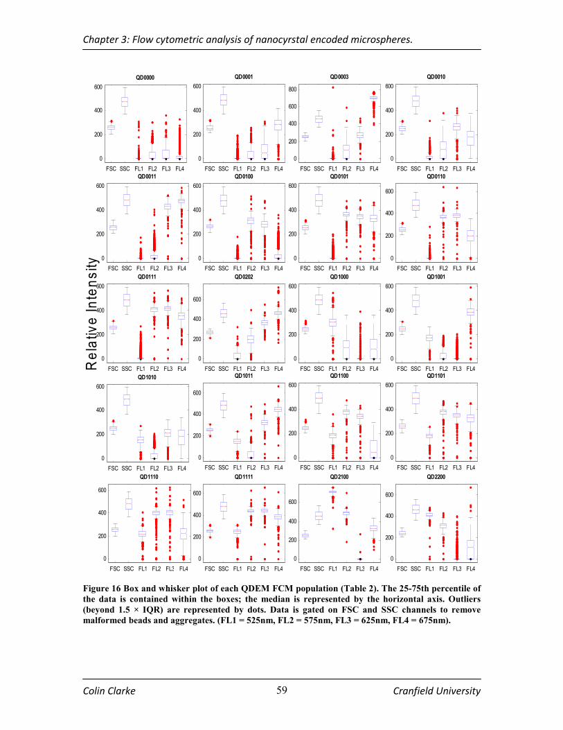
Chapter 3: Flow cytometric analysis of nanocyrstal encoded microspheres.
Colin Clarke Cranfield University 59
FSC SSC FL1 FL2 FL3 FL4
0
200
400
600
QD0000
FSC SSC FL1 FL2 FL3 FL4
0
200
400
600
QD0001
FSC SSC FL1 FL2 FL3 FL4
0
200
400
600
800
QD0003
FSC SSC FL1 FL2 FL3 FL4
0
200
400
600
QD0010
FSC SSC FL1 FL2 FL3 FL4
0
200
400
600
QD0011
FSC SSC FL1 FL2 FL3 FL4
0
200
400
600
QD0100
FSC SSC FL1 FL2 FL3 FL4
0
200
400
600
QD0101
FSC SSC FL1 FL2 FL3 FL4
0
200
400
600
QD0110
FSC SSC FL1 FL2 FL3 FL4
0
200
400
600
QD0111
FSC SSC FL1 FL2 FL3 FL4
0
200
400
600
QD0202
FSC SSC FL1 FL2 FL3 FL4
0
200
400
600
QD1000
FSC SSC FL1 FL2 FL3 FL4
0
200
400
600
QD1001
FSC SSC FL1 FL2 FL3 FL4
0
200
400
600
QD1010
FSC SSC FL1 FL2 FL3 FL4
0
200
400
600
QD1011
FSC SSC FL1 FL2 FL3 FL4
0
200
400
600
QD1100
FSC SSC FL1 FL2 FL3 FL4
0
200
400
600
QD1101
FSC SSC FL1 FL2 FL3 FL4
0
200
400
600
QD1110
FSC SSC FL1 FL2 FL3 FL4
0
200
400
600
QD1111
FSC SSC FL1 FL2 FL3 FL4
0
200
400
600
QD2100
FSC SSC FL1 FL2 FL3 FL4
0
200
400
600
QD2200
Relative Intensity
Figure 16 Box and whisker plot of each QDEM FCM population (Table 2). The 25-75th percentile of
the data is contained within the boxes; the median is represented by the horizontal axis. Outliers
(beyond 1.5 × IQR) are represented by dots. Data is gated on FSC and SSC channels to remove
malformed beads and aggregates. (FL1 = 525nm, FL2 = 575nm, FL3 = 625nm, FL4 = 675nm).
Chapter 3: Flow cytometric analysis of nanocyrstal encoded microspheres.
Colin Clarke Cranfield University 60
Evaluation of multiparameter gating
The first of the classification methods, MPG (section 3.4.1), was employed to
differentiate QDEMs from the multiplex testing set (Table 4). A combination gate was
defined by manually “drawing” a gate around each of the individual QDEM
subpopulations on bivariate histograms and then linking the gates over multiple
parameters using Boolean logic (Figure 17). The FCSexpress FCM software suite was
used to accomplish this task. To compensate for possible errors in MPG due to outliers
the regions were manually tuned to attempt to select the QDEM gates that yielded the
lowest misclassification on the training data. Defining the gates required for the QDEM
library was a complex, subjective and time consuming process (~45 min), which
increases exponentially as the numbers of codes are increased. These concerns would be
exacerbated at higher levels of multiplexing with additional QDs and intensity levels. To
assess the accuracy of MPG the multiplex QDEM solution data (Table 4) was presented
to the combination gates.
Shown below are the number of events recorded for each of the ten tests (an allocation of
500 events per QDEM set), the first point to note about MPG classification results is
there are more classifications made on the data than events recorded on the flow
cytometer (Table 5). Thus certain events are classified as belonging to two or more
populations. Even with painstaking adjustment in order to optimise the gates, the
optimum regions for each QDEM were not defined. As stated above the MC rate was
used to evaluate the results on the mixture solutions as the actual classes of events were
not known.

Chapter 3: Flow cytometric analysis of nanocyrstal encoded microspheres.
Colin Clarke Cranfield University 61
FL1 LOG
FL2 LOG
100
101
102
103
104
100
101
102
103
104
FL3 LOG
FL4 LOG
100
101
102
103
104
100
101
102
103
104
Figure 17 Combination gating of QDEM library. Each of the twenty gates is set individually on each
microsphere population. The gates were adjusted to give the best performance on each individual
microsphere population. The population is shown above is QD1111, the empty gates were defined the
other populations in sequence. Future mixed subpopulation FCM data can then be presented to the
gates for classification.
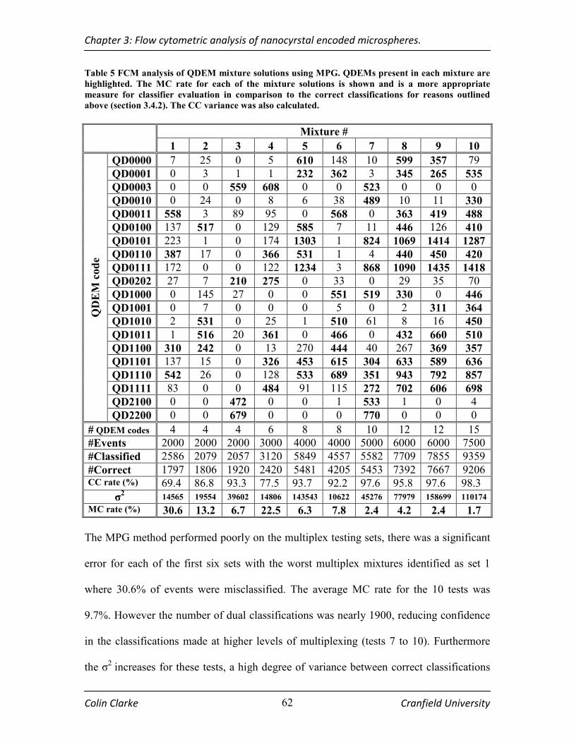
Chapter 3: Flow cytometric analysis of nanocyrstal encoded microspheres.
Colin Clarke Cranfield University 62
Table 5 FCM analysis of QDEM mixture solutions using MPG. QDEMs present in each mixture are
highlighted. The MC rate for each of the mixture solutions is shown and is a more appropriate
measure for classifier evaluation in comparison to the correct classifications for reasons outlined
above (section 3.4.2). The CC variance was also calculated.
Mixture #
1 2 3 4 5 6 7 8 9 10
QD0000 7 25 0 5 610 148 10 599 357 79
QD0001 0 3 1 1 232 362 3 345 265 535
QD0003 0 0 559 608 0 0 523 0 0 0
QD0010 0 24 0 8 6 38 489 10 11 330
QD0011 558 3 89 95 0 568 0 363 419 488
QD0100 137 517 0 129 585 7 11 446 126 410
QD0101 223 1 0 174 1303 1 824 1069 1414 1287
QD0110 387 17 0 366 531 1 4 440 450 420
QD0111 172 0 0 122 1234 3 868 1090 1435 1418
QD0202 27 7 210 275 0 33 0 29 35 70
QD1000 0 145 27 0 0 551 519 330 0 446
QD1001 0 7 0 0 0 5 0 2 311 364
QD1010 2 531 0 25 1 510 61 8 16 450
QD1011 1 516 20 361 0 466 0 432 660 510
QD1100 310 242 0 13 270 444 40 267 369 357
QD1101 137 15 0 326 453 615 304 633 589 636
QD1110 542 26 0 128 533 689 351 943 792 857
QD1111 83 0 0 484 91 115 272 702 606 698
QD2100 0 0 472 0 0 1 533 1 0 4
QD
EM
co
de
QD2200 0 0 679 0 0 0 770 0 0 0
# QDEM codes 4 4 4 6 8 8 10 12 12 15
#Events 2000 2000 2000 3000 4000 4000 5000 6000 6000 7500
#Classified 2586 2079 2057 3120 5849 4557 5582 7709 7855 9359
#Correct 1797 1806 1920 2420 5481 4205 5453 7392 7667 9206 CC rate (%) 69.4 86.8 93.3 77.5 93.7 92.2 97.6 95.8 97.6 98.3
σ2 14565 19554 39602 14806 143543 10622 45276 77979 158699 110174
MC rate (%) 30.6 13.2 6.7 22.5 6.3 7.8 2.4 4.2 2.4 1.7
The MPG method performed poorly on the multiplex testing sets, there was a significant
error for each of the first six sets with the worst multiplex mixtures identified as set 1
where 30.6% of events were misclassified. The average MC rate for the 10 tests was
9.7%. However the number of dual classifications was nearly 1900, reducing confidence
in the classifications made at higher levels of multiplexing (tests 7 to 10). Furthermore
the σ2 increases for these tests, a high degree of variance between correct classifications

Chapter 3: Flow cytometric analysis of nanocyrstal encoded microspheres.
Colin Clarke Cranfield University 63
suggest that false positive results are present (Figure 18) and the number of QDEMs in
solution masked the performance of gating, (i.e. misclassified events are more likely to
fall into a present microsphere gate as additional QDEMs are added). It is more likely
that multiplex solutions 1-6 reflect the true performance of the classification method, the
average MC rate for these solutions was 14.5%.
3.5 Improving on MPG – the case for research
The limitations of MPG were shown for the identification of QDEMs. The MPG
accuracy was questionable for the mixture solutions (Figure 18) with an average MC rate
of 9.7% observed. Results on the solutions containing 10 or more QDEMs where the MC
rate decreases should be treated with caution as the variance between the correct
classification increases.
1 2 3 4 5 6 7 8 9 100
5
10
15
20
25
30
35
MC rate %
Mixture #
MC rate
CC Variance
0
2
4
6
8
10
12
14
16x 10
4
CC Variance
Figure 18 Performance of the MPG for the ten mixture sets. The MC rate of the gating system for
each test is shown in descending order. The average MC rate was 9.7%. The CC variance of
classifications on solutions containing more QDEMs is increased suggesting misclassifications within
these solutions.

Chapter 3: Flow cytometric analysis of nanocyrstal encoded microspheres.
Colin Clarke Cranfield University 64
Moreover a large number of dual classifications were observed, these were the result of
classes lying on the decision boundaries (gates). The technique was also time-consuming,
requiring the interpretation of a skilled operator; and there was no assurance that the
optimum regions had been defined.
When the number of parameters increases the number bivariate plots required increases
exponentially and the interpretation of plots becomes more difficult. The classification
accuracy of the MPG would decrease further, moreover MPG be would become even
more complex and time consuming. Hence utility of graphical methods such as MPG in
polychromatic FCM analysis of QDEMs is limited, and these methods are unsuitable for
extension of encoded microsphere populations required for bioanalytical studies. It is on
this rationale that this work is based; in the following chapters two supervised learning
algorithms are applied to investigate accurate automated discrimination of QDEMs of
single events in FCM to improve upon the performance of MPG.
Recently a number of machine learning algorithms for multivariate pattern recognition
have been applied for FCM subpopulation identification. The remainder of this thesis
describes the construction and evaluation of two popular supervised learning methods,
SVMs and ANNs. Such techniques would allow automation and optimisation of the MPG
in multidimensional space, and remove the subjectivity of user defined classification
boundaries. Moreover these methods would allow the majority of FCM instrumentation
present in a wide variety of locations, such as the EPICS XL to remain viable for SAT.

Chapter 4: Support vector machines for the
identification of QDEMs from FCM data.
Chapter 4: Support vector machines for the identification of QDEMs from FCM data.
Colin Clarke Cranfield University 66
4.1 Introduction
Chapter 3 demonstrated the need for improvement in current methods of QDEM
classification. The overall aim of this research was the development of a rapid automated
classification method for QDEMs overcoming the limitations of multiparameter gating
and unsupervised methods. To this end, multivariate supervised techniques (such as
SVMs and ANNs) offer a novel solution worthy of further investigation. In this chapter
the theory of supervised learning (section 4.2.1), SVMs (section 4.2.2) and multiclass
SVM implementations (section 4.2.3) are described. SVMs are used in a wide range of
applications including bioinformatics and biospectroscopy [134-136], and several
examples of such methods for the identification of subpopulations from FCM data are
presented (section 4.2.4). The methodology for the construction and performance
evaluation of an SVM classifier for QDEMs is presented (section 4.3) and the
comparison of the SVM to MPG described in chapter 3 discussed (section 4.4).
4.2 Support vector machines
4.2.1 Supervised learning
Supervised learning techniques are trained on previous examples with known
classifications thus “learning” the underlying patterns within the data; such models are
then applied to previously unknown examples in order to make a prediction. Pattern
recognition models construct a classification rule from known examples (training data) to
recognise unknown examples. Given a training set consisting of input and output pairs,
( ) ( ) ( ){ }ii yxyxyxZ ,,...,,,, 2211= , the aim of training is to produce a function f which maps

Chapter 4: Support vector machines for the identification of QDEMs from FCM data.
Colin Clarke Cranfield University 67
the input vectors Xx∈ to the corresponding class labels Yy ∈ to allow the prediction of
unknown samples. SVM and ANN are examples of popular supervised learning
algorithms, the following section details SVM theory while chapter 5 deals with ANNs.
4.2.2 Fundamentals of support vector machines
SVMs are a widely used supervised learning algorithm developed by Vapnik [137]. The
popularity of SVMs stems from advantages such as the use of kernels for non-linearly
separable data (known as the kernel trick), no local minima, sparseness of the solution,
and capacity control (important for good generalisation) obtained by optimising the
decision boundary in the margin between classes [136, 137]. SVMs have been shown to
outperform similar supervised classification methods such as artificial neural networks
and linear discriminant analysis (LDA) in many instances due to a high generalisation
ability (ability to classify unknown samples) and robustness to high dimensional data
[136].
In terms of classification, for a linearly separable two class problem with class labels +1
and -1, SVMs locate a boundary of separation (hyperplane) to identify the two classes. A
generalised hyperplane function is shown below (Eqn 4.1) [138].
bxwxf +⋅=)( (4.1)
Where w is termed the weight vector and b is the bias.

Chapter 4: Support vector machines for the identification of QDEMs from FCM data.
Colin Clarke Cranfield University 68
While SVMs share similarities with linear discriminant analysis and perceptrons which
also aim to find the separating hyperplane between two classes, the use of simple
hyperplanes in LDA and perceptrons is limited as a unique solution does not exist. The
best separating hyperplane may not be found as there may be many hyperplanes that
separate the data (Figure 19), decreasing the classifiers generalisation ability [136].
Figure 19 Many hyperplanes can be located for any given dataset. LDA suffers from drawbacks in
that the best decision boundary may not be found. SVM overcomes this through optimisation of the
maximal margin hyperplane (see below).
SVMs calculate the optimum hyperplane (maximal margin hyperplane) yielding the best
generalisation, avoiding overfitting (memorising the training data, thus unseen examples
may be misclassified) (Figure 20). The maximal margin hyperplane is determined from
X by minimizing the norm of w by means of a constrained optimisation by
minimisation of a quadratic function under linear equality constraints (Eqn 4.2) [136].
Minimize: 2
2
1w
Such that: ( ) ii bxwyi 1≥+⋅ for ,,....1 ni =
(4.2)

Chapter 4: Support vector machines for the identification of QDEMs from FCM data.
Colin Clarke Cranfield University 69
Figure 20 Representation of the SVM solution applied to a linearly separable two class problem. The
classes are shown as red diamonds and green circles. The hyperplane is shown as a dark black line.
Support vectors (SV) (see below) for each class are shown as blanks shapes.
Location of the maximal margin classifier alone does not take into account the training
error of the dataset leaving the SVM susceptible to the effects of noise; as a result more
robust margin methods that can tolerate noise, outliers and consider more training points
apart from those on the margin were developed. The so-called slack variables and penalty
parameter are introduced (Eqn 4.3) allowing the margin to be crossed creating a “soft”
hyperplane. The penalty parameter C punishes outliers during the training process and
controls the trade off between training errors and model complexity. Slack variables, iξ
are introduced to allow the margin constraints to be overcome during optimisation to
avoid overfitting to noisy data [136, 137].
Minimize: ∑=
+n
i
iCw1
2,ξ
Such that: ( ) ii bxwyi ξ−≥+⋅ 1 and 0≥iξ for ,,....1 ni =
(4.3)

Chapter 4: Support vector machines for the identification of QDEMs from FCM data.
Colin Clarke Cranfield University 70
The resulting decision function is illustrated below (Eqn 4.4), where the constants iα are
called Lagrange multipliers and are determined during the optimisation of the SVM. SV
are the support vectors, for which iα > 0, which lie closest to the optimal hyperplane. For
the remaining patterns the iα = 0.
( ) ∑∈
+⋅=svx
iii
i
bxxyxf α (4.4)
The above hypothesis holds only for linearly separable data, many applications in real
world analysis tend to be of a non-linear nature. LDA is limited in this regard and failures
of the perceptron were exposed by Minsky and Papert in the 1960s [139], leading to the
development of multilayer neural networks (see chapter 5).
SVMs however employ kernels to map the data to a high dimensional feature space
where the examples become linearly separable and the SVM classification can proceed
(Figure 21) [136-138]. Choosing the correct SVM kernel is similar to the choice of ANN
architecture and is critical to model performance [136], there are a number of commonly
used kernels (Eqn 4.5-4.8) and custom functions can also be written for a particular
application. Perhaps one of the main advantages in terms of the application of SVMs is
that by using kernels the learning algorithm can be decoupled from the application area.
Classification in the high dimensional feature space is not, however without
complications, computational expense increases due to the large vectors and high
dimensionality may cause overfitting, however SVMs offset any decrease in
generalisation ability of the classifier through location of the maximal margin classifier
[138].
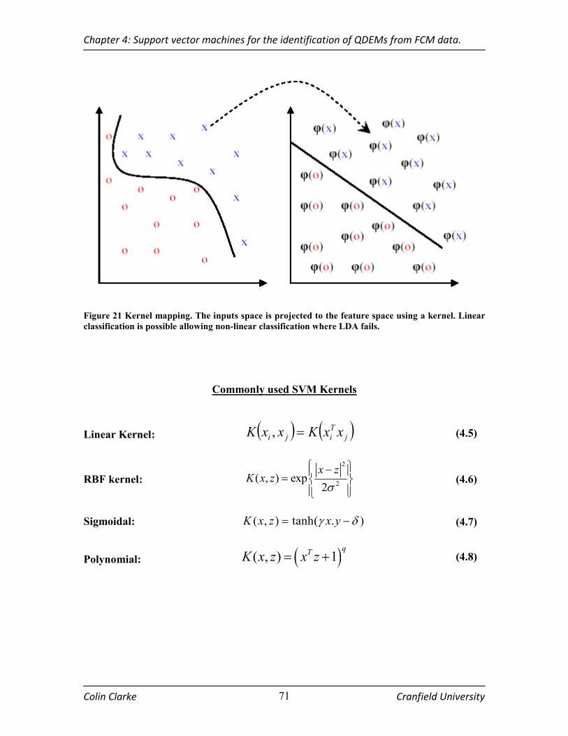
Chapter 4: Support vector machines for the identification of QDEMs from FCM data.
Colin Clarke Cranfield University 71
Figure 21 Kernel mapping. The inputs space is projected to the feature space using a kernel. Linear
classification is possible allowing non-linear classification where LDA fails.
Commonly used SVM Kernels
Linear Kernel: ( ) ( )j
T
iji xxKxxK =, (4.5)
RBF kernel:
2
2( , ) exp
2
x zK x z
σ
− =
(4.6)
Sigmoidal: ( , ) tanh( . )K x z x yγ δ= − (4.7)
Polynomial: ( )( , ) 1q
TK x z x z= + (4.8)

Chapter 4: Support vector machines for the identification of QDEMs from FCM data.
Colin Clarke Cranfield University 72
4.2.3 Multiclass support vector machines
Thus far only binary SVMs capable of separating two classes from one another have been
considered; however a classification system for QDEMs requires the identification of
multiple classes. Various approaches have been utilised for extension of the SVM
formulation to all classes such as the Vapnik and Weston approach which aims to solve
the multiclass problem using a single optimisation [140], [141], binary trees and fuzzy
logic methods are also suggested in the literature but so far all have had limited success
due to time consuming implementation, the requirement of a priori knowledge and the
use of clustering or vector quantisation algorithms to determine classifier hierarchy [142,
143]. For multiclass problems several methods exist that combine binary SVM classifiers
to create multiclass SVMs. The most popular schemes are the one versus rest (OVR), and
the one versus one (OVO) method using majority voting and pairwise coupling [140,
144]. In this thesis only the OVR and OVO methods are employed, it is important to note
several other methods exist but the methods outlined above have had the greatest success
[145].
The OVR approach and OVO are two common methods of error output coding (ECOC)
[146]. When combining binary SVMs an ECOC scheme is used to combine classifier
outputs to yield the final prediction. For a K -class problem; when a pattern is classified
an output vector is produced by the SVM, this output vector consists of the output from K
classifiers and the vector is subsequently mapped to the predicted label. Majority voting
(cumulative number of classifications by each SVM) is the basis of class decision; the
class which receives the most “votes” is the final class decision for the sample.
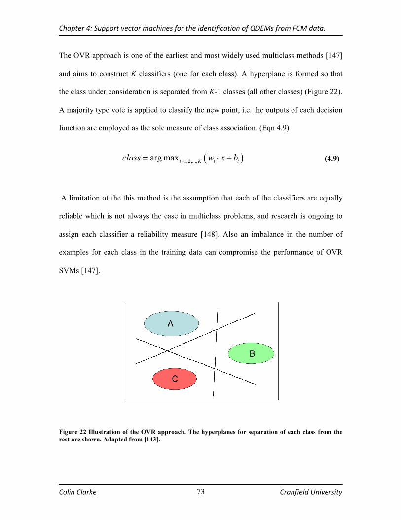
Chapter 4: Support vector machines for the identification of QDEMs from FCM data.
Colin Clarke Cranfield University 73
The OVR approach is one of the earliest and most widely used multiclass methods [147]
and aims to construct K classifiers (one for each class). A hyperplane is formed so that
the class under consideration is separated from K-1 classes (all other classes) (Figure 22).
A majority type vote is applied to classify the new point, i.e. the outputs of each decision
function are employed as the sole measure of class association. (Eqn 4.9)
( )1,2,...,arg maxi K i iclass w x b== ⋅ + (4.9)
A limitation of the this method is the assumption that each of the classifiers are equally
reliable which is not always the case in multiclass problems, and research is ongoing to
assign each classifier a reliability measure [148]. Also an imbalance in the number of
examples for each class in the training data can compromise the performance of OVR
SVMs [147].
Figure 22 Illustration of the OVR approach. The hyperplanes for separation of each class from the
rest are shown. Adapted from [143].

Chapter 4: Support vector machines for the identification of QDEMs from FCM data.
Colin Clarke Cranfield University 74
OVO multiclass SVMs create a classifier for each pair of classes resulting in 2/)1( −KK
classifiers (Figure 23); each classifier is trained to separate between any two classes ),( ji .
The result is a K × K matrix where the classification is made by simply summing each
row of the matrix for which the sum is maximal (Eqn 4.10):
,maxarg1
,...,1
= ∑
==
K
jKi
fijclass (4.10)
Where, fij is the signed confidence measure for the ij ’th classifier [146]. While the
number of individual classifiers is greater than the OVO method, the individual training
problems are significantly smaller and may also save on training time. Furthermore the
runtime execution of the OVO multiclass SVM is decreased as there is less overlap
between classes and individual SVMs require a smaller number of SVs for
discrimination. However as stated above the output of different binary classifiers may not
be directly comparable as classes may be of different sizes and or less separable from the
rest of the data.
Figure 23 Illustration of the one versus all approach. An SVM is formed for each pair of classes.
Adapted from [143].

Chapter 4: Support vector machines for the identification of QDEMs from FCM data.
Colin Clarke Cranfield University 75
4.2.4 Previous examples of SVM and flow cytometry data
Interest is growing for pattern recognition techniques in the FCM community as a result
of increasing numbers of FCM parameters (more complex analysis), concerns over
subjective gating [149] and the advent of flow based post-genomic assays [5]. There are a
number of examples reported in the literature for the automated analysis of FCM data
with SVMs improving upon traditional FCM data analysis in clinical diagnostics and
research. Toedling et al. recently demonstrated the use of SVMs in the clinical setting. A
radial basis SVM was constructed to automate the classification of leukemic cells from
acute lymphoblastic leukaemia patients and compared to a traditional gating method
performed by a skilled analyst. The SVM required no control sample group from healthy
patients. There was a 99.06% agreement between analyst and SVM; moreover
sensitivities of 99.78% and specificity of 98.87% were reported.
The classification of various types of white blood cells was demonstrated by Adjouadi et
al. Samples from normal and abnormal patients could be identified with 95% and 86.67%
accuracy respectively [150]. Quinn et al. described the use of a SVM for the
identification of cellular viability and lineage in bone marrow cells. In this instance the
optimum classifier was found to be an RBF ANN, the SVM misclassified 9.4% ± 2.8% in
comparison to MPG; and 6.4% ± 1.3% for the neural network [151]. Analysis of highly
variable complex phytoplankton data with SVMs has also been shown to be an effective
data analysis method. RBF SVMs were utilised for the recognition of 60 species with a
mean accuracy of 90% for each species, outperforming an RBF ANN by 13% [150, 152,
153].

Chapter 4: Support vector machines for the identification of QDEMs from FCM data.
Colin Clarke Cranfield University 76
4.3 Materials and methods
4.3.1 SVM training data preparation
The dataset for this study consisted of 1,000 FCM events, for each spectrally unique
QDEM, excluding QD1100, of which there were 796 events. The data set described in the
previous chapter 3 is therefore a 19,796 × 6 matrix (two scatter intensity and four
fluorescence intensity measurements [FSC, SSC, FL1@525nm, FL2@575nm,
FL3@625nm and FL4@675nm]), and forms the training data for the SVM. QDEMs were
analysed individually and the identity of each event in the training data was known,
allowing the application of supervised learning methods for classification. See chapter 3
for more information on acquisition of the training data.
Each of the 20 LMD files containing the training data was imported into MATLAB. Mild
and extreme outliers resulting from inherent FCM variation and/or variation in QDEM
manufacture were removed beyond 1.5 times the interquartile range (IQR) of each
parameter [154], reducing the training set by 1,242 events (6.27% of the total events).
The effect of removing the mild and extreme outliers from the training dataset was
determined.
Building an SVM classifier has three main phases; parameter selection, training and
independent test set validation. The training data and corresponding class labels were
randomised and divided to form the cv_set (25%), train_set (50%) and test_set (25%)
providing independent data for each of the respective phases (Figure 24). The datasets
were then converted to sparse data format files for input to the LIBSVM program (section
4.3.2).
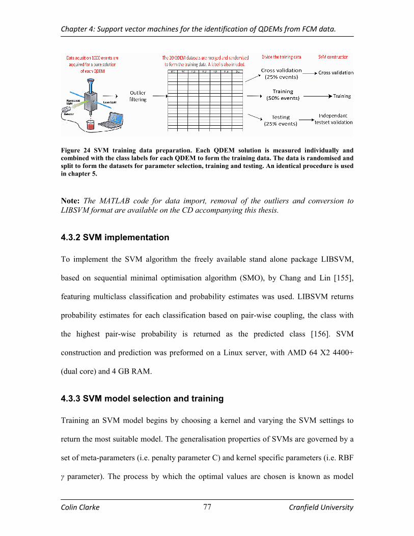
Chapter 4: Support vector machines for the identification of QDEMs from FCM data.
Colin Clarke Cranfield University 77
Figure 24 SVM training data preparation. Each QDEM solution is measured individually and
combined with the class labels for each QDEM to form the training data. The data is randomised and
split to form the datasets for parameter selection, training and testing. An identical procedure is used
in chapter 5.
Note: The MATLAB code for data import, removal of the outliers and conversion to
LIBSVM format are available on the CD accompanying this thesis.
4.3.2 SVM implementation
To implement the SVM algorithm the freely available stand alone package LIBSVM,
based on sequential minimal optimisation algorithm (SMO), by Chang and Lin [155],
featuring multiclass classification and probability estimates was used. LIBSVM returns
probability estimates for each classification based on pair-wise coupling, the class with
the highest pair-wise probability is returned as the predicted class [156]. SVM
construction and prediction was preformed on a Linux server, with AMD 64 X2 4400+
(dual core) and 4 GB RAM.
4.3.3 SVM model selection and training
Training an SVM model begins by choosing a kernel and varying the SVM settings to
return the most suitable model. The generalisation properties of SVMs are governed by a
set of meta-parameters (i.e. penalty parameter C) and kernel specific parameters (i.e. RBF
γ parameter). The process by which the optimal values are chosen is known as model
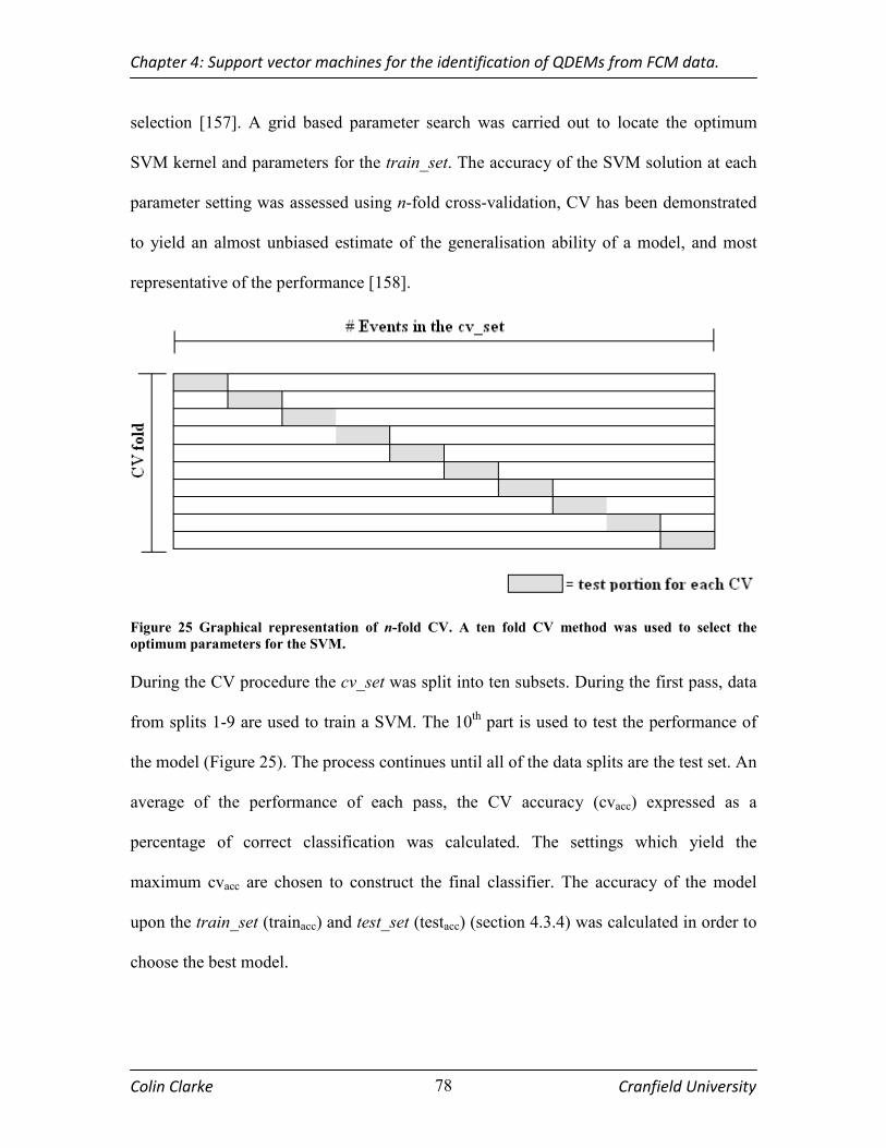
Chapter 4: Support vector machines for the identification of QDEMs from FCM data.
Colin Clarke Cranfield University 78
selection [157]. A grid based parameter search was carried out to locate the optimum
SVM kernel and parameters for the train_set. The accuracy of the SVM solution at each
parameter setting was assessed using n-fold cross-validation, CV has been demonstrated
to yield an almost unbiased estimate of the generalisation ability of a model, and most
representative of the performance [158].
Figure 25 Graphical representation of n-fold CV. A ten fold CV method was used to select the
optimum parameters for the SVM.
During the CV procedure the cv_set was split into ten subsets. During the first pass, data
from splits 1-9 are used to train a SVM. The 10th part is used to test the performance of
the model (Figure 25). The process continues until all of the data splits are the test set. An
average of the performance of each pass, the CV accuracy (cvacc) expressed as a
percentage of correct classification was calculated. The settings which yield the
maximum cvacc are chosen to construct the final classifier. The accuracy of the model
upon the train_set (trainacc) and test_set (testacc) (section 4.3.4) was calculated in order to
choose the best model.

Chapter 4: Support vector machines for the identification of QDEMs from FCM data.
Colin Clarke Cranfield University 79
CV was carried out using the Linear and RBF kernel to create linear and non-linear
solutions for QDEM classification. For the linear kernel the penalty parameter, C, is
varied, however with the RBF kernel C and the width of the RBF function, γ, is also
varied in order to construct the optimum SVM. The penalty parameter was varied from 1
× 10-6 to 10 with the linear kernel and RBF kernel. The γ parameter was also varied for
the RBF kernel from 1 × 10⁻⁴ to 50. The effect of removal of outliers was investigated,
and the OVR and OVO multiclass SVM designs were also compared. Once the best
solution was determined, the train_set was used to train the appropriate SVM model.
4.3.4 SVM validation
An independent validation of the SVM was carried out using the previously unseen
test_set. From the test_set predictions a confusion matrix was plotted to determine the
performance of each individual class [159]. A confusion matrix allowed the behaviour of
each individual class within the entire classification model to be observed. The well
known indicators accuracy, specificity and sensitivity/recall (see below) were calculated
from the independent test_set confusion matrix for each QDEM class. Firstly accuracy is
defined as the probability that a random event will be classified correctly (See Eqn 4.11).
Specificity can be defined as the probability of correct negative prediction (See Eqn
4.12). Sensitivity can be defined as the probability of correct positive classification (Eqn
4.13). Both sensitivity and sensitivity are calculated for each individual class considered
by the model.

Chapter 4: Support vector machines for the identification of QDEMs from FCM data.
Colin Clarke Cranfield University 80
( )
TP TNAccuracy
TP TN FP FN
+=
+ + + (4.11)
( )TN
Specificity STN FP
=+
(4.12)
( )TP
Sensitivity RTP FN
=+
(4.13)
Where:
TP = True positives - the number of QDEMs labelled correctly.
FP = False positives - the number of QDEMs incorrectly labelled.
TN = True negatives - number of QDEMs correctly predicted not to be the specified
QDEM.
FN = False negatives - number of QDEM predictions that were classified as negative
but were actually positive [160, 161].
These performance measures are more likely to reflect the actual performance (and
overfitting risk) when applied to examples not seen in the training set. As a further
measure of the SVM, the classifications on the multiplex testing sets described in the
previous chapter were presented to the classifier. The multiplex test solutions were
acquired independently of the training data reveal the ability of the SVM to discriminate
multiple QDEMs in a single solution acting as an external validation of the model. The
resulting MC rate for these external testing set were calculated for the direct comparison
to MPG described in chapter 3.
Note: See the CD accompanying this thesis for MATLAB code to construct confusion
matrices and calculate the performance indicators.

Chapter 4: Support vector machines for the identification of QDEMs from FCM data.
Colin Clarke Cranfield University 81
4.4 Results and discussion
The following section describes the results obtained during the construction and
evaluation of an SVM for QDEM recognition. The optimum kernel and SVM parameters
are selected for the dataset (section 4.4.1 SVM parameter selection, the effect of outlier
removal on SVM performance is investigated (section 4.4.2), and the OVO and OVR
SVM multiclass methods compared (section 4.4.3). The selected model performance is
further demonstrated through independent test set validation (section 4.4.5) and an
external validation with the multiplex tests (section 4.4.6). Finally the SVM is compared
to the MPG method outlined in chapter 3 (section 4.4.6).
4.4.1 SVM parameter selection
The primary step in model selection was the identification of the most suitable kernel.
From the outset it was observed that the polynomial and sigmoidal kernels had a higher
computational expense and classification rates were poor (~30% less than linear and RBF
kernels), therefore parameter selection for only the linear and RBF kernels was conducted
to construct the optimum model for classification of the QDEM dataset in both linear and
non-linear SVM modes. CV was performed for each SVM parameter combination to
determine the optimum settings for the model. The train and test accuracies were also
calculated as additional indicators. In the case of SVM linear kernel the penalty
parameter C was varied from 1 × 10⁻⁶ to 10. RBF SVM parameters were also examined in
the same manner as the linear kernel; C was chosen first and varied over the same range
as the linear kernel. Once C had been identified, the width of the RBF function (γ) was
varied from 1 × 10⁻⁴ to 50.
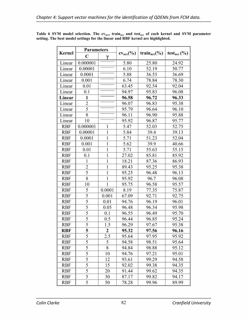
Chapter 4: Support vector machines for the identification of QDEMs from FCM data.
Colin Clarke Cranfield University 82
Table 6 SVM model selection. The cvacc, trainacc and testacc of each kernel and SVM parameter
setting. The best model settings for the linear and RBF kernel are highlighted.
Parameters Kernel
C γ cvacc(%) trainacc(%) testacc (%)
Linear 0.000001 ------------- 5.80 25.80 24.92
Linear 0.00001 ------------- 6.10 52.19 50.77
Linear 0.0001 ------------- 5.88 36.53 36.69
Linear 0.001 ------------- 6.74 78.84 78.30
Linear 0.01 ------------- 63.45 92.54 92.04
Linear 0.1 ------------- 94.97 95.83 96.08
Linear 1 -------------
96.58 96.72 96.33
Linear 2 ------------- 96.07 96.83 95.38
Linear 5 ------------- 95.79 96.64 96.10
Linear 8 ------------- 96.11 96.90 95.88
Linear 10 ------------- 95.92 96.87 95.77
RBF 0.000001 1 5.47 52.03 52.75
RBF 0.00001 1 5.84 39.4 39.13
RBF 0.0001 1 5.71 51.23 52.04
RBF 0.001 1 5.62 39.9 40.66
RBF 0.01 1 5.71 55.63 55.15
RBF 0.1 1 27.02 85.81 85.92
RBF 1 1 18.21 87.36 86.93
RBF 2 1 89.43 95.25 95.38
RBF 5 1 95.25 96.48 96.13
RBF 8 1 95.92 96.7 96.08
RBF 10 1 95.75 96.58 95.57
RBF 5 0.0001 8.19 77.35 75.87
RBF 5 0.001 67.09 92.71 92.75
RBF 5 0.01 94.76 96.19 96.01
RBF 5 0.05 96.48 96.34 95.98
RBF 5 0.1 96.55 96.49 95.70
RBF 5 0.5 96.44 96.85 95.24
RBF 5 1.5 96.29 97.67 95.38
RBF 5 2 95.32 97.56 96.16
RBF 5 2.5 95.64 97.95 95.92
RBF 5 5 94.58 98.51 95.64
RBF 5 8 94.84 98.88 95.12
RBF 5 10 94.76 97.21 95.01
RBF 5 12 93.61 99.29 94.58
RBF 5 15 92.02 99.38 94.35
RBF 5 20 91.44 99.62 94.35
RBF 5 30 87.17 99.82 94.17
RBF 5 50 78.28 99.96 89.99
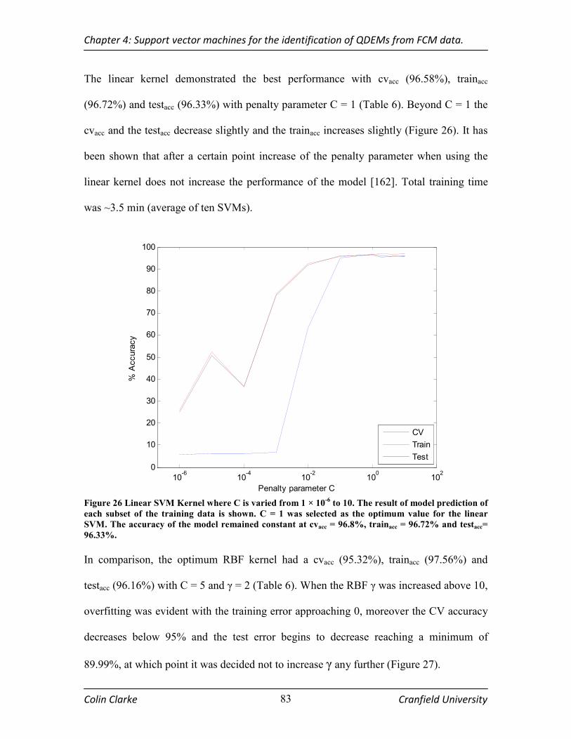
Chapter 4: Support vector machines for the identification of QDEMs from FCM data.
Colin Clarke Cranfield University 83
The linear kernel demonstrated the best performance with cvacc (96.58%), trainacc
(96.72%) and testacc (96.33%) with penalty parameter C = 1 (Table 6). Beyond C = 1 the
cvacc and the testacc decrease slightly and the trainacc increases slightly (Figure 26). It has
been shown that after a certain point increase of the penalty parameter when using the
linear kernel does not increase the performance of the model [162]. Total training time
was ~3.5 min (average of ten SVMs).
10-6
10-4
10-2
100
102
0
10
20
30
40
50
60
70
80
90
100
Penalty parameter C
% Accuracy
CV
Train
Test
Figure 26 Linear SVM Kernel where C is varied from 1 × 10
-6 to 10. The result of model prediction of
each subset of the training data is shown. C = 1 was selected as the optimum value for the linear
SVM. The accuracy of the model remained constant at cvacc = 96.8%, trainacc = 96.72% and testacc=
96.33%.
In comparison, the optimum RBF kernel had a cvacc (95.32%), trainacc (97.56%) and
testacc (96.16%) with C = 5 and γ = 2 (Table 6). When the RBF γ was increased above 10,
overfitting was evident with the training error approaching 0, moreover the CV accuracy
decreases below 95% and the test error begins to decrease reaching a minimum of
89.99%, at which point it was decided not to increase γ any further (Figure 27).

Chapter 4: Support vector machines for the identification of QDEMs from FCM data.
Colin Clarke Cranfield University 84
10-4
10-3
10-2
10-1
100
101
102
0
10
20
30
40
50
60
70
80
90
100
RBF width ( γ )
% Accuracy
CV
Train
Test
Figure 27 RBF SVM Kernel, C = 5 (Table 4) (the optimum penalty parameter), γ is varied between 1
× 10-4
to 50. The resulting of model prediction of each subset of the training data is shown.
Overfitting is evident beyond γ = 10 the CV and test accuracies decrease, the training accuracy
increases. The optimum RBF accuracies were cvacc = 95.32%, trainacc = 97.6% and testacc = 96.16%.
The classification rates of the two SVMs are very similar. The RBF SVM can
approximate both linear and non-linear problems and has been shown to have
performance comparable to the linear kernel; therefore achieving similar results for both
SVMs is not surprising. While LDA or partial least square discriminant analysis
(PLSDA) could have been used for this dataset, maximal margin optimisation and the
option of non-linear extension to the classification scheme in the future gives the SVM
advantages over both methods. The training time for the RBF kernel was slightly greater
requiring ~5mins in comparison to ~3.5mins for linear SVM training. As new QDEMs
are added to the model the training time is expected to increase (using the OVR
multiclass design the number of binary SVMs increasing the training time would increase
exponentially (section 4.4.3)).

Chapter 4: Support vector machines for the identification of QDEMs from FCM data.
Colin Clarke Cranfield University 85
The RBF kernel required a greater number of SVs (2230) compared to the linear kernel
(944) to define the SVM decision boundaries. An increase in the numbers of SVs
increases the computational cost of the SVM model during prediction. For QDEMs
analysed in a high throughput format, FCM is capable of detection rates of 1000 events
per second, the number of calculations required for single event classification are 44%
less for the linear kernel. The number of SVs is proportional to the complexity of the
separating hypersurface. The authors of the LIBSVM package advise that the linear
kernel be chosen following Occam’s razor, the simplest model is best, and the model
with the fewest SVs was chosen (i.e. the linear kernel with the lowest geometric decision
surface complexity ) [163].
Therefore a SVM incorporating a linear kernel, with C = 1 was found to yield the highest
CV accuracy with the shortest training time and fewest support vectors. These settings
were used in the construction SVMs to determine the suitability of outlier removal and
the comparison between OVO and OVR. However application of the RBF must not be
discounted for future studies as increases in the coding complexity QDEMs may require a
non linear kernel. The performance of the RBF kernel demonstrates the flexibility of
SVMs for pattern recognition tasks.
4.4.2 Outlier removal suitability
The suitability of outlier removal process for SVM training by means of the IQR was
determined by constructing an SVM for training data with and without outliers and
determining the accuracies on each training data split. The number of outliers removed
for each class is shown below (Figure 28).

Chapter 4: Support vector machines for the identification of QDEMs from FCM data.
Colin Clarke Cranfield University 86
600
650
700
750
800
850
900
950
1000# Events
QD0000
QD0000
QD0000
QD0000
QD0001
QD0001
QD0001
QD0001
QD0003
QD0003
QD0003
QD0003
QD0010
QD0010
QD0010
QD0010
QD0011
QD0011
QD0011
QD0011
QD0100
QD0100
QD0100
QD0100
QD0101
QD0101
QD0101
QD0101
QD0110
QD0110
QD0110
QD0110
QD0111
QD0111
QD0111
QD0111
QD0202
QD0202
QD0202
QD0202
QD1000
QD1000
QD1000
QD1000
QD1001
QD1001
QD1001
QD1001
QD1010
QD1010
QD1010
QD1010
QD1011
QD1011
QD1011
QD1011
QD1100
QD1100
QD1100
QD1100
QD1101
QD1101
QD1101
QD1101
QD1110
QD1110
QD1110
QD1110
QD1111
QD1111
QD1111
QD1111
QD2100
QD2100
QD2100
QD2100
QD2200
QD2200
QD2200
QD2200
Outliers Retained
Figure 28 Post acquisition outlier removal for each QDEM. A total of 1242 events were removed. The
remaining events were retained to form the training data.
Following outlier removal an increase in the cvacc from 91.10% to 96.58% was observed,
moreover the number SVs required to separate the 20 classes decreased from 2145 to 944
reducing model complexity and increasing the classification speed of the SVM (Table 7).
The test set accuracy increased by 3.31%. The removal of outliers from the training data
is a reliable method which does not affect the generalisation ability, hence outlier filtered
training data is used for the remainder of this thesis.
Table 7 Suitability of outlier removal using the optimum SVM configuration. An SVM was trained
and tested for the QDEM dataset before and after the removal of outliers.
#Samples
Training Test CV Kernel C cvacc(%)
False
Positives
(test)
testacc(%)
+Outliers 9900 4948 4948 Linear 1 91.10% 345 93.02%
-Outliers 9277 4638 4638 Linear 1 96.58% 155 96.33%

Chapter 4: Support vector machines for the identification of QDEMs from FCM data.
Colin Clarke Cranfield University 87
4.4.3 Evaluation of multiclass SVM designs
To determine the optimum multiclass SVM design, a comparison of the suitability of the
OVR and OVO methods (section 4.2.2) for the QDEM dataset was investigated. Cross
validation, training and testing were performed and the cvacc, trainacc and testacc calculated
for both multiclass designs (Table 8).
Table 8 Comparison of the OVR and OVO multiclass SVM methods. The CV, train and test
accuracy for each SVM are shown.
cvacc (%) trainacc (%) testacc (%) #SV
OVR 75.24 89.44 89.52 8107
OVO 96.58 96.72 96.33 944
The OVO method clearly out performs these methods and therefore it was decided to use
OVO for the SVM. The literature suggests that OVO has a greater performance and the
results here support those assertions [145]. A drawback of both the OVO and OVR
method is that for any given sample the significance of each classification is weighted
equally, while it is impossible to know the classifiers significance, certain classifiers are
redundant and can be removed with a so-called mixture matrix [164].
The final design of the classifier was an OVO multiclass SVM employing the linear
kernel, with a penalty parameter C = 1, trained and evaluated on outlier filtered FCM
data. The performance of the model had cvacc = 96.58%, trainacc = 96.72%, and an
independent test validation; testacc = 96.33%. These results demonstrate the potential of
the SVMs for QDEM recognition in FCM.

Chapter 4: Support vector machines for the identification of QDEMs from FCM data.
Colin Clarke Cranfield University 88
4.4.4 SVM performance with increasing QDEMs
The effect of increasing the number of QDEMs per SVM was also investigated as a
possible measure of the capacity of this approach when the future numbers of QDEMs
increase. The effect of adding classes to the model was assessed beginning with two
QDEM populations. To avoid class bias in the evaluation (where the most or least
separable classes are considered), 10 individual classifiers were constructed containing n
random classes for each QDEM number considered and the average cvacc, trainacc and
testacc calculated (Table 9).
Table 9 Evaluation of the effect of addition of QDEMs on test set accuracy. An individual SVM was
constructed for each test.
#QDEM cvacc (%) trainacc (%) testacc (%)
2 99.67 99.68 99.69
3 99.75 99.84 99.78
4 99.55 99.60 99.43
5 99.29 99.39 99.33
6 98.69 98.82 98.44
7 98.43 98.57 98.36
8 98.26 98.59 98.43
9 98.65 98.76 98.59
10 97.68 97.97 97.79
11 97.56 97.84 97.66
12 97.63 97.95 98.05
13 97.75 98.06 97.61
14 97.05 97.48 96.95
15 96.91 97.42 97.04
16 96.98 97.30 97.00
17 96.72 97.05 96.70
18 96.14 96.58 96.48
19 96.23 96.68 96.28
20 96.58 96.72 96.33

Chapter 4: Support vector machines for the identification of QDEMs from FCM data.
Colin Clarke Cranfield University 89
2 4 6 8 10 12 14 16 18 2096
96.5
97
97.5
98
98.5
99
99.5
100
QDEM per SVM
Accuracy (%)
CV
train
test
Figure 29 Evaluation of the effect of increasing the number of classes considered by the SVM.
A decrease in the accuracy in the classification of the unseen data (testacc = 3.67%) can be
observed between the 2 class and 20 class model. It is thought that the SVM should
eventually become independent of the number of QDEM classes as the OVO multiclass
design creates an individual set of binary classifiers for each QDEM, therefore
complexity (number of SVs) required for each binary classifier does not increase. As the
number of QDEMs increases the accuracy would be expected to decrease (as the
encoding complexity across the QDEM library is considered) and remain constant. In
comparison the addition of classes with the OVR approach would increase the
complexity of the decision boundaries as each binary SVM separates a class from all
other classes. More QDEM types are required to further investigate the SVM beyond 20
QDEMs and it remains a concern.
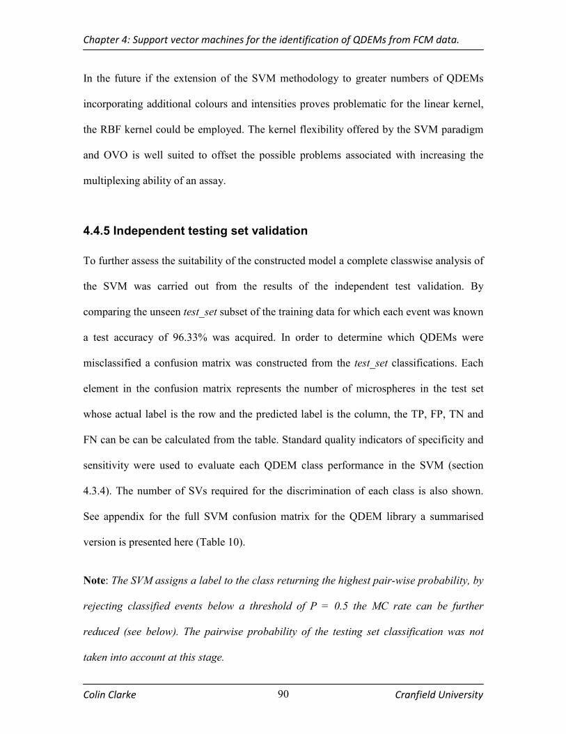
Chapter 4: Support vector machines for the identification of QDEMs from FCM data.
Colin Clarke Cranfield University 90
In the future if the extension of the SVM methodology to greater numbers of QDEMs
incorporating additional colours and intensities proves problematic for the linear kernel,
the RBF kernel could be employed. The kernel flexibility offered by the SVM paradigm
and OVO is well suited to offset the possible problems associated with increasing the
multiplexing ability of an assay.
4.4.5 Independent testing set validation
To further assess the suitability of the constructed model a complete classwise analysis of
the SVM was carried out from the results of the independent test validation. By
comparing the unseen test_set subset of the training data for which each event was known
a test accuracy of 96.33% was acquired. In order to determine which QDEMs were
misclassified a confusion matrix was constructed from the test_set classifications. Each
element in the confusion matrix represents the number of microspheres in the test set
whose actual label is the row and the predicted label is the column, the TP, FP, TN and
FN can be can be calculated from the table. Standard quality indicators of specificity and
sensitivity were used to evaluate each QDEM class performance in the SVM (section
4.3.4). The number of SVs required for the discrimination of each class is also shown.
See appendix for the full SVM confusion matrix for the QDEM library a summarised
version is presented here (Table 10).
Note: The SVM assigns a label to the class returning the highest pair-wise probability, by
rejecting classified events below a threshold of P = 0.5 the MC rate can be further
reduced (see below). The pairwise probability of the testing set classification was not
taken into account at this stage.
Chapter 4: Support vector machines for the identification of QDEMs from FCM data.
Colin Clarke Cranfield University 91
Table 10 Independent test Set validation, true positives (#TP), specificity (S) and sensitivity (R) are
shown. See appendix 1 for the SVM confusion matrix. Test set accuracy = 96.33%. The number of
support vectors (#SVs) is shown for each class. The least sensitive class is highlighted.
ID #TP S (%) R (%) #SV
1 QD0000 233 99.8 92.8 68
2 QD0001 223 99.6 94.9 65
3 QD0003 260 99.9 100 10
4 QD0010 210 99.8 94.5 65
5 QD0011 234 99.7 97.9 25
6 QD0100 225 100 97.4 22
7 QD0101 216 99.9 89.3 121
8 QD0110 211 99.9 92.5 102
9 QD0111 229 99.6 93.4 85
10 QD0202 205 100 98.0 36
11 QD1000 241 100 99.5 19
12 QD1001 222 99.8 99.1 19
13 QD1010 212 99.6 95.9 48
14 QD1011 210 99.6 99.5 22
15 QD1100 164 99.4 93.1 60
16 QD1101 226 99.9 97.8 77
17 QD1110 218 100 93.5 87
18 QD1111 254 100 97.3 35
19 QD2100 223 100 100 6
20 QD2200 224 100 100 15
The lowest sensitivity observed was for QD0101(R=89.3%) and resulted from a degree
of confusion between QD0101, QD0110 (R= 92.5%) and QD0111 (R=93.4%). The
confusion between these classes may have been due to the 620nm QD not being centred
over the 625nm emission filter for optimum performance. The remaining QDEM classes
perform well with sensitivity of >90% for the entire 19 classes. The microsphere QD0000
was expected to have a higher sensitivity (R = 92.8%) as this microsphere had no
emission. The cause of the low sensitivity is not known, one possibility is that a small
amount of blank QDEMs were present in the remaining QDEM solutions leading to
misclassification in the independent test set validation. All QDEM classes returned
excellent specificity (S > 99%).
Chapter 4: Support vector machines for the identification of QDEMs from FCM data.
Colin Clarke Cranfield University 92
As stated previously QD1100 had the fewest instances in the training set containing lower
concentration of QDEM in the stock solution. The specificity and sensitivity of these
QDEMs was 99.4% and 93.1% respectively, suggesting that the imbalance in the number
of events for each QDEM has no effect on SVM performance.
4.4.6 Performance on the multiplexed testing sets
While the performance on the training data was excellent, an additional test was
conducted to see how the SVM would perform using multiple QDEMs in a single
solution (Table 11), forming an external validation of the model. No outlier filtering was
carried out on these results (the IQR filtering method only works with single population
QDEM datasets) so it was assumed that these datasets would contain similar noise to the
pre-filtered training data. Post classification removal of these outliers was accomplished
using the prediction pairwise probability provided by LIBSVM.
For the reasons outlined in section 3.4.2 the success of the SVM was measured by
calculating the MC rate and σ2. The table shows the number of classified events
belonging to each QDEM. Events were rejected as unclassified results when the pairwise
class probabilities were ≤ 0.5, resulting in between 0.1 and 5.2% rejection for each of the
tests. The MC rate was calculated for each of the 10 multiplexed test sets (simply the
number of false positives divided by total events remaining after probability filtering).
Test four yielded the highest number of misclassifications at 6.4%.

Chapter 4: Support vector machines for the identification of QDEMs from FCM data.
Colin Clarke Cranfield University 93
Table 11 Prediction of unknown events from test samples using SVM classifier. The number of
misclassifications (p ≤ 0.5) is shown for each QDEM (See Table 2 for test set composition).
Test#
1 2 3 4 5 6 7 8 9 10
QD0000 7 20 0 5 554 94 7 570 340 52
QD0001 0 0 1 1 318 448 4 398 298 563
QD0003 0 0 568 618 0 0 533 0 0 0
QD0010 4 9 0 9 10 20 560 12 15 419
QD0011 559 1 22 14 0 571 0 355 410 475
QD0100 8 530 0 11 426 3 21 321 22 305
QD0101 6 2 0 1 423 1 147 277 407 388
QD0110 497 12 0 448 709 1 17 573 625 534
QD0111 32 0 0 27 523 0 708 592 762 833
QD0202 10 1 231 287 0 5 1 16 18 25
QD1000 1 14 3 0 0 467 498 328 0 349
QD1001 0 0 0 0 0 1 0 0 287 358
QD1010 1 538 0 32 1 522 5 11 23 419
QD1011 1 554 1 428 0 504 1 455 662 490
QD1100 182 247 0 3 80 231 5 75 237 222
QD1101 1 0 0 234 218 318 135 320 319 338
QD1110 653 26 0 83 554 677 415 909 726 723
QD1111 16 2 1 697 25 24 501 600 532 641
QD2100 0 0 683 0 0 0 778 0 0 0
QD
EM
co
de
QD2200 0 0 487 0 0 11 574 14 0 10
# QDEM codes 4 4 4 6 8 8 10 12 12 15
#Events 2000 2000 2000 3000 4000 4000 5000 6000 6000 7500
#Classified 1978 1956 1997 2898 3841 3898 4910 5826 5683 7144
Rejected (%) 1.1 2.2 0.1 3.4 3.9 2.5 1.8 2.9 5.2 4.7
#Correct 1891 1869 1969 2712 3725 3738 4849 5698 5605 7057 CC rate (%) 95.7 95.6 98.6 93.6 97 95.9 98.8 97.9 98.7 98.8
σ2 41684 21660 36801 32584 23520 19653 43722 33235 34551 27389
MC rate (%) 4.3 4.4 1.4 6.4 3.0 4.1 1.2 2.1 1.3 1.2
On increasing the rejection criteria to p = 0.75 the misclassification decreases to 0.2%,
while the rejection rate increases to 16.3% of total events (data not shown). The SVM
performed well on the remaining test sets with the MC rate below 4.5%. The 15 QDEM
had the lowest MC rate demonstrating the ability of the SVM to discriminate between the
lowest intensity microspheres (level 1 intensity). For test 3 only multiple intensity ratio

Chapter 4: Support vector machines for the identification of QDEMs from FCM data.
Colin Clarke Cranfield University 94
beads were used. The SVM accurately identified the four multiple intensity QDEMs with
only 1.4% misclassifications for test 3. The average MC rate for each of multiplex test
sets was 2.9% with an average rejection rate of 2.7%. For tests 1-6 the average MC rate
was 3.9%. For each mixture set the top predicted QDEMs corresponded exactly to those
QDEMs present in the test solution. QD1100 was also predicted at a lower rate in the
multiplexed testing, further suggesting that the stock concentration was originally lower.
Misclassifications may be due to confusion between classes, detector overspill or
instrumental drift. The use of narrower bandwidth emission filters could reduce cross talk
between detectors and centering of the FL3 channel at 620nm should decrease the levels
of misclassification in the SVM. The variance of the CCs for each multiplex solution
were similar, there was no significant increase in the variance when the individual
QDEMs in the solution were increased providing a greater confidence in the accuracy of
classifications for mixtures 7-10.
4.5 Conclusion
The aim of this chapter was to improve the accuracy of QDEM identification from FCM
data reported in chapter 3. In that chapter, a MPG method was used to classify each
QDEM by means of selecting regions from a series of 2D plots. The methods suffered
from an inability to find the optimum gates for classification due to overlap between
QDEM signatures resulting in multiple classifications for a single event and >30%
misclassification for the most difficult microspheres to classify. In comparison the
supervised learning paradigm of SVMs, has been shown to outperform MPG in every
multiplex test (Figure 30). While MPG analysis returned <2% misclassifications for Test

Chapter 4: Support vector machines for the identification of QDEMs from FCM data.
Colin Clarke Cranfield University 95
10, 1859 extra classifications were made than events recorded (this was also the case for
other tests), moreover there was an increase in the variance of CCs calling into question
the validity of the MPG results and therefore the suitability of the technique. The MPG
method is also time consuming and as the number of QDEMs increases it becomes more
so, moreover the optimum gates may not be found.
1 2 3 4 5 6 7 8 9 100
5
10
15
20
25
30
Mixture #
MC rate (%)
MPG
SVM
Figure 30 Comparison of MPG (multiparameter gating) and SVM MC rates. The SVM outperforms
MPG in all tests. Demonstrating the potential of SVM for the discrimination of QDEMs from SVM
and supervised learning algorithms (For a comparison of the variance of CCs see Figure 45).
SVMs have been shown to be a highly accurate means of QDEM analysis, the technique
trains rapidly (average training time 3.5mins), moreover the probability of classification
can be taken into account and results filtered from the data. SVMs are capable of forming
gates in a kernel induced feature space, the algorithm locates the optimum decision
boundary between classes by locating the maximum margin hyperplane (section
4.2.1).The SVM reported here has shown excellent specificity (average R = 96.33%),
sensitivity (average S = 99.82%), and an overall classification accuracy of 96.33% on
Chapter 4: Support vector machines for the identification of QDEMs from FCM data.
Colin Clarke Cranfield University 96
unseen data. Moreover the SVM model preformed well in external validation;
demonstrating reduced MC rate for the QDEMs present in each solution in comparison to
MPG (Figure 30). The variance of CCs with the SVM model remained relatively constant
for the SVM in comparison to those of the MPG across the 10 external validation
solutions (Figure 45). Average SVM σ2 = 31479 in comparison to σ2 = 63482 for MPG.
In comparison to a commercial SAT analysis, the Luminex platform, a classification rate
is quoted as >80% [165]. The average 3% MC rate using our SVM model, compared to
Luminex misclassification of less than 2%, test 4 had a MC rate of 6.4%, however the
Luminex system combines dual organic dyes and a more complex microsphere encoding
scheme is used here. Concerns still exist as to the suitability of SVMs for the scaling up
of QDEM libraries. The OVO design should be robust and SVM can operate both in
linear and non-linear modes which may be advantageous when additional microspheres
are added.
SVMs are theoretically well suited to the automatic gating of flow cytometry
subpopulations. SVM can be thought of taking the “flow cytometry input space” and
using the maximal margin hyperplane to gate the data in a multidimensional feature space
to produce optimum classification of QDEMs subpopulations for SAT, the results shown
here confirm this.
In the following chapter a comparison between the SVM and another supervised learning
algorithm, artificial neural networks is carried out. ANNs have also proved effective for
FCM subpopulations in the past thus it is prudent to compare these classification methods
to the SVM.

Chapter 5: Development of a neural network based
QDEM classification system.

Chapter 5: Development of a neural network based QDEM classification system.
Colin Clarke Cranfield University 98
5.1 Overview
Chapter 4 described the successful application of multiclass SVMs to the classification of
QDEMs from FCM data. This chapter aims to compare the SVM to artificial neural
network classifiers (section 5.2.1). These supervised methods have had reasonable
success in FCM (section 5.2.2). Two popular ANN architectures (section 5.3) were
constructed using the QDEM data and evaluated using an independent test set validation
and external validation for comparison to the SVM classifier.
5.2 Introduction
5.2.1 Artificial neural networks
An artificial neural network is a machine learning technique loosely based on biological
nervous systems such as the brain [166, 167]. The origins of ANNs date back to the
1940s, with the description of simplified neurons by McCulloch and Pitts [168], and
subsequent development of the perceptron for two class discrimination by Frank
Rosenblatt in 1956 [169]. However the failures of the single layer perceptron model in
some basic pattern recognition tasks were demonstrated by Minsky and Papert, leading to
a decrease in the pace of research lasting until the 80’s. The field was revived through the
work of Hopkins who demonstrated the use of ANNs for real world applications [170],
and the development of the back propagation learning algorithm for multilayer
perceptrons [171].

Chapter 5: Development of a neural network based QDEM classification system.
Colin Clarke Cranfield University 99
Today neural networks are a computationally efficient, easily constructed, non-
parametric method which assumes no a priori knowledge of the data under examination
and are well accepted in many branches of science and engineering for applications such
as pattern classification, function approximation, image processing and many others
[166].
Figure 31 Model of an ANN neuron.
ANNs are composed of a collection of linked processing units (neurons) (Figure 31);
each neuron obtains inputs from the external environment and from other neurons in the
network. Connections between the processing units are weighted and each input has a
weight, w associated with it. The response (output) of each unit is calculated through
some function f of the weighted sum of its inputs (Equation 5.1):
i ij i
j
y f w x
= ∑ (5.1)
Where iy is the output of the neuron. The weighted sum ij i
j
w x∑ is termed the net input
to the ith unit and is also called inet . The function f is termed the activation function and
governs how the neuron processes input signals to produce an output. The activation
function weights the value of the output, often between 1 and 0 or between -1 and 1

Chapter 5: Development of a neural network based QDEM classification system.
Colin Clarke Cranfield University 100
depending on the type of activation function used. The activation function introduces
non-linearity into the network. Examples of common activation including the step
function, Gaussian and the popular sigmiodal activation functions are shown below
(Figure 32) [167].
Figure 32 Neuron activation functions. (A) Identity function (B) Step function (C) sigmoid function.
The neurons are divided into processing layers of which there are generally three main
types. Firstly an input layer which connects the ANN to data environment under study, a
hidden layer models the data distribution and the output layer which delivers the identity
of each class. As stated above an ANN is an interlinked structure of neurons; the
arrangement of neurons, layers and the connections between them is termed the ANN
architecture e.g. feed-forward, recurrent or self organising maps (SOM). With the feed
forward design the data flow between input and output neurons is only allowed to
propagate directly through the network; there are no looped connections. Recurrent
architectures can contain connections between the nodes in the same layer or nodes in the
previous layers of the network. In the hidden layer of a SOM nodes are arranged into a
rectangular or hexagonal lattice, each of which are fully connected to the input layer and
define a topographical position.
(A) (B) (C)

Chapter 5: Development of a neural network based QDEM classification system.
Colin Clarke Cranfield University 101
Combinations of single one-class networks known as ANN ensembles or stacked neural
networks (SNN) are also suitable for classification. While some success has been
demonstrated, such ensembles suffer from the lack of interaction between single
networks during the learning phase and the way the networks are combined increasing
the possibility of individual networks not contributing to the classification [172].
Therefore the ANNs employed in this thesis were single networks trained on all classes
simultaneously. For a detailed discussion of ANN architectures see [166].
ANN training aims to create a predictive model by configuring a network such that the
presentation of a set of input values produces the desired set of outputs. The initial weight
vectors for the ANN are chosen randomly and in supervised ANN training the weights
are adjusted according to response of data patterns. The updating of weights in an ANN is
determined by learning rules, of which there are four basic types, error-correction,
Boltzmann, Hebbian, and competitive learning.
While this chapter concentrates on supervised paradigms (section 4.2.1) ANN training
can be either supervised or unsupervised. Examples of unsupervised networks include the
Kohonen’s SOM [167], and Hopfield networks [170]. There also exists a hybrid method
where both supervised learning and unsupervised learning are combined, with part of the
weights are usually determined through supervised learning, while others are determined
through unsupervised learning [173]. The specific characteristics and learning methods of
the selected ANNs for this study are detailed below (section 5.3). For an excellent review
of training methods for ANNs see [167] and [166].

Chapter 5: Development of a neural network based QDEM classification system.
Colin Clarke Cranfield University 102
5.2.2 Previous applications in flow cytometry
To date a number of examples of the application of ANNs to classification of microalgae
from FCM data have been reported in the literature [174-177]. Boddy et al. previous
work illustrates the application of ANNs to FCM for the identification of phytoplankton
species from 11-parameter data. Radial basis function neural networks (section 5.3.2)
were trained to recognize 35-70 species of phytoplankton. The best performing RBF
network could correctly identify 91.5% of phytoplankton after training using gradient
descent algorithm [176]. The identification of fungal spores using flow cytometry and
artificial neural networks has also been reported previously [178] [179].
Quinn et al. has recently described a pattern recognition methodology for the
classification of live, apoptotic (programmed cell death) stage and dead cells from FCM
data based on ANNs. FSC and SSC measurements relate to cell size and granularity and
are indicators of the morphological changes that cells undergo during apoptosis. Lecours
dual staining method with 7-aminoactinomycin D (7AAD) and annexin V was utilised to
determine cell lineage and the developmental stage. Traditional data analysis was used to
set gates to define the intensity threshold for these dyes to locate live, apoptotic and dead
cells, cells positive for 7AAD are designated as dead (degradation of the cellular
membrane allows access to nuclear DNA resulting in an increase in binding). Cells
positive for annexin V but negative for 7AAD are designated as apoptotic, and finally
cells with observed negative populations for both dyes are “live”. The gates were defined
by an expert panel of analysts resulting in variations between users particularly at the
boundaries between populations. Both supervised and unsupervised ANNs were
evaluated consisting of multilayer perceptron, radial basis function (RBF), recurrent
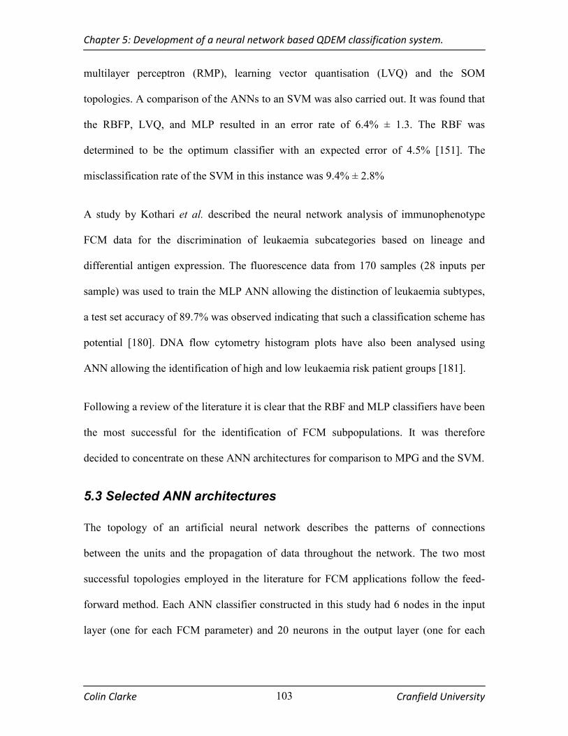
Chapter 5: Development of a neural network based QDEM classification system.
Colin Clarke Cranfield University 103
multilayer perceptron (RMP), learning vector quantisation (LVQ) and the SOM
topologies. A comparison of the ANNs to an SVM was also carried out. It was found that
the RBFP, LVQ, and MLP resulted in an error rate of 6.4% ± 1.3. The RBF was
determined to be the optimum classifier with an expected error of 4.5% [151]. The
misclassification rate of the SVM in this instance was 9.4% ± 2.8%
A study by Kothari et al. described the neural network analysis of immunophenotype
FCM data for the discrimination of leukaemia subcategories based on lineage and
differential antigen expression. The fluorescence data from 170 samples (28 inputs per
sample) was used to train the MLP ANN allowing the distinction of leukaemia subtypes,
a test set accuracy of 89.7% was observed indicating that such a classification scheme has
potential [180]. DNA flow cytometry histogram plots have also been analysed using
ANN allowing the identification of high and low leukaemia risk patient groups [181].
Following a review of the literature it is clear that the RBF and MLP classifiers have been
the most successful for the identification of FCM subpopulations. It was therefore
decided to concentrate on these ANN architectures for comparison to MPG and the SVM.
5.3 Selected ANN architectures
The topology of an artificial neural network describes the patterns of connections
between the units and the propagation of data throughout the network. The two most
successful topologies employed in the literature for FCM applications follow the feed-
forward method. Each ANN classifier constructed in this study had 6 nodes in the input
layer (one for each FCM parameter) and 20 neurons in the output layer (one for each

Chapter 5: Development of a neural network based QDEM classification system.
Colin Clarke Cranfield University 104
individual QDEM). The following section describes both the MLP and RBF type
networks in detail.
5.3.1 Feed forward multilayer perceptrons
As stated above single perceptron neurons have limited ability in classification problems,
the combination of perceptrons arranged in layers however is a much more powerful
learning technique. MLPs are the most popular ANN described today in the literature. An
MLP “may be viewed as a practical vehicle for performing a nonlinear input-output
mapping of a general nature” [182]. These highly connective (each neuron is connected
to every neuron in the previous layer) feed-forward architectures calculate a weighted
sum of their inputs, and pass the activation level through the network to produce the
output.
Figure 33 Multilayer perceptron.

Chapter 5: Development of a neural network based QDEM classification system.
Colin Clarke Cranfield University 105
For any given layer the neurons receive their input from the previous layer on the input
side of their network and their output to the following layer on the output side, there are
no interlayer connections (Figure 33). The first layer is known an as the input layer. The
input signal is modified by the initial weights jpw and the bias 1b resulting in an input to
the thj neuron in the hidden layer (j =1, 2, 3) of jnet , which is a weighted input of the
intensity values [166, 183].
The hidden layers are activation functions of the weighted inputs plus a bias, the output
of the hidden layer is then distributed to any other hidden layers until the output units are
reached. Based on the equation above the output of the thj neuron in the hidden layer is:
The training method employed for MLPs in this work is known as the back propagation
algorithm [184, 185]. The network weights are updated with respect to the classification
error calculated upon input of the previous training set, the learning rate and the
magnitude of the output.
1
N
i i i
i
y f w x b=
= ⋅ +
∑ (5.2)
( )j H jy f net= (5.3)

Chapter 5: Development of a neural network based QDEM classification system.
Colin Clarke Cranfield University 106
The back propagation algorithm, a type of error correction learning is defined as a
gradient descent method to minimize the squared error cost function [166], an error signal
is then back-propagated from the output layer to the hidden layer and the network is
altered. Back propagation consists of two passes throughout the various layers of the
MLP, a forward pass and backward pass. During the forward pass, an input pattern is
applied to the nodes of the network, and its effect propagates through the network layer
by layer producing an output signal. While the weights remain fixed during the forward
pass of the training algorithm, during the backward pass the weights are adjusted in order
to reduce the error. The back propagation algorithm is an iterative process, on each
iteration or epoch the training set is presented to the network. The weights in the network
are updated according to the degree of classification error, the magnitude of the output
and the learning rate, η . Once a predefined threshold, for example the desired CVacc or a
set number of iterations is reached training terminates. A representation of the decision
boundaries formed by an MLP is shown below (Figure 34).
Figure 34 Representation of MLP separation of a two QDEM problem in 2-dimensional space.

Chapter 5: Development of a neural network based QDEM classification system.
Colin Clarke Cranfield University 107
5.3.2 Radial basis function networks
RBF ANNs can be considered as a special type of multilayer feed forward network using
of a number of locally tuned neurons [186-188]. A RBF is composed of a single hidden
layer, with linear output functions (there is also a bias on each output node) and nonlinear
transfer functions [166]. There are no weights in the hidden layer, the outputs of the
hidden units are in fact calculated using the “closeness” of the input to some positive
radially symmetric function (a kernel) [183]. A RBF ANN has a hidden layer of radial
units e.g. Gaussian (Figure 35), this single hidden layer is sufficient for any application
due to the non-linearity of the radial unit function. While MLP units are defined by their
weights and threshold, radial units are defined by the central point and radius. Each node
in the hidden layer represents a kernel function and each output node calculates the
weighted sum of the hidden layer outputs [188].
The kernel function output is determined by its centre and width, the output is high when
close to the centre and decreases rapidly toward zero as the input distance from the centre
increases. Gaussian functions are popular in the literature and have been shown to be
successful in FCM subpopulation classification [151].
The Gaussian hidden layer function is given by:
Where σ and µ are the width and centres of the thj node in the hidden layer. jZ is the
output. A summation of each output node gives the response of the network for a given
input.
2
2( ) exp ,
2
j
j
j
XZ x
µ
σ
− = −
(5.4)

Chapter 5: Development of a neural network based QDEM classification system.
Colin Clarke Cranfield University 108
Figure 35 Radial Basis Function: Hidden layer nodes use Gaussians of varying standard deviations to
determine the output.
While MLPs classify a given pattern by means of hyperplanes, RBF ANNs divide up the
input space by considering the distribution of the data under consideration (Figure 37).
Training a RBF ANN is different to the training of MLPs in that there is no updating of
the weights after each pass. Training of the RBF hidden node kernel is achieved through
the selection of the function centres and widths using a cross validation procedure, finally
the hidden-to-output weights are calculated. Selection of the radial function can be
thought of as defining the optimum number of basis functions.
The training of RBF neural networks occurs in two separate stages; an unsupervised
routine such as K-means clustering can be used to determine the centres of the basis
functions [189], for more information see [183]. The second stage involves a simple least
mean squares (LMS) optimisation or singular value decomposition to calculate the
weights for the output layer of the network [190]. Further improvement in the
classification performance of the network has been reported using a gradient descent
method to simultaneously adjust the basis function and weights.
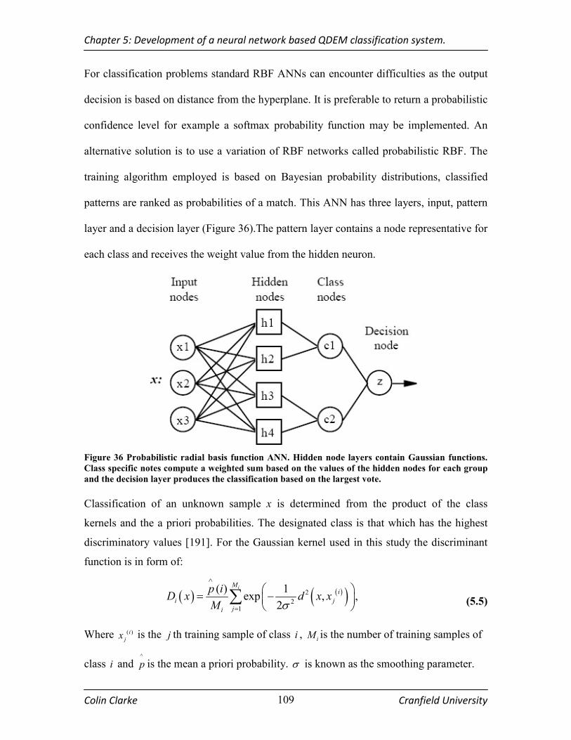
Chapter 5: Development of a neural network based QDEM classification system.
Colin Clarke Cranfield University 109
For classification problems standard RBF ANNs can encounter difficulties as the output
decision is based on distance from the hyperplane. It is preferable to return a probabilistic
confidence level for example a softmax probability function may be implemented. An
alternative solution is to use a variation of RBF networks called probabilistic RBF. The
training algorithm employed is based on Bayesian probability distributions, classified
patterns are ranked as probabilities of a match. This ANN has three layers, input, pattern
layer and a decision layer (Figure 36).The pattern layer contains a node representative for
each class and receives the weight value from the hidden neuron.
Figure 36 Probabilistic radial basis function ANN. Hidden node layers contain Gaussian functions.
Class specific notes compute a weighted sum based on the values of the hidden nodes for each group
and the decision layer produces the classification based on the largest vote.
Classification of an unknown sample x is determined from the product of the class
kernels and the a priori probabilities. The designated class is that which has the highest
discriminatory values [191]. For the Gaussian kernel used in this study the discriminant
function is in form of:
( ) ( )( )2
21
( ) 1exp , ,
2
iMi
i j
ji
p iD x d x x
M σ
∧
=
= −
∑ (5.5)
Where ( )i
jx is the j th training sample of class i ,
iM is the number of training samples of
class i and ^
p is the mean a priori probability. σ is known as the smoothing parameter.
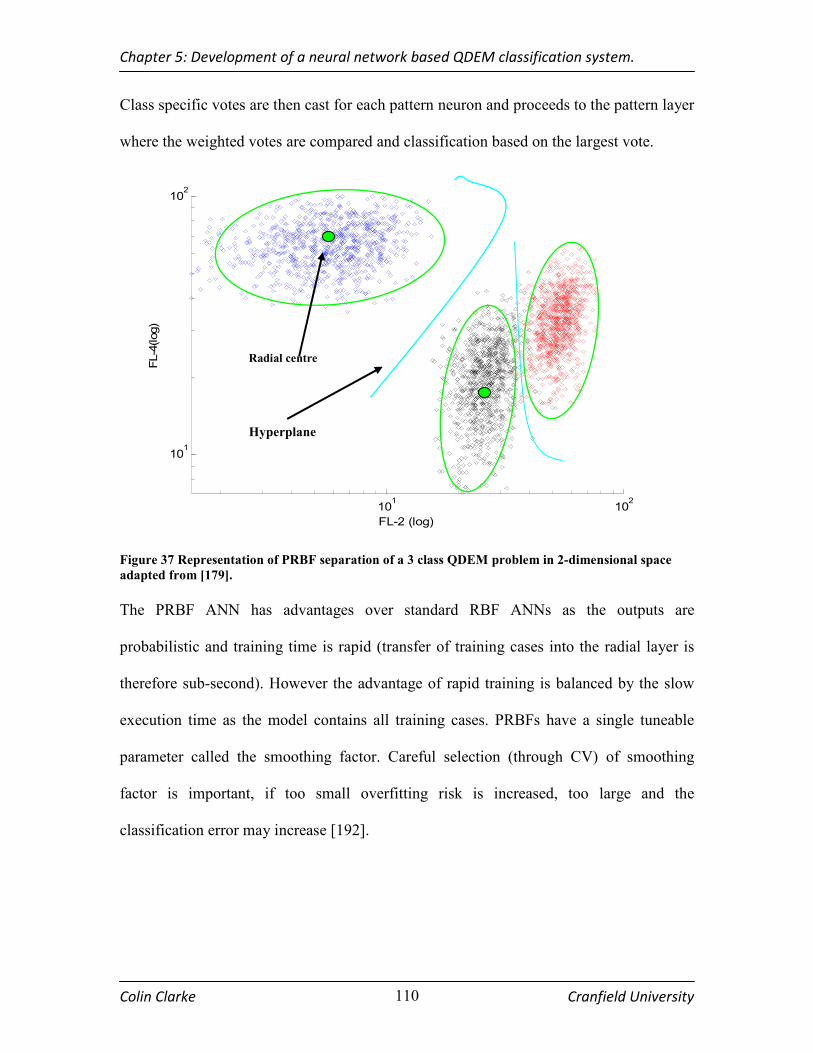
Chapter 5: Development of a neural network based QDEM classification system.
Colin Clarke Cranfield University 110
Class specific votes are then cast for each pattern neuron and proceeds to the pattern layer
where the weighted votes are compared and classification based on the largest vote.
Figure 37 Representation of PRBF separation of a 3 class QDEM problem in 2-dimensional space
adapted from [179].
The PRBF ANN has advantages over standard RBF ANNs as the outputs are
probabilistic and training time is rapid (transfer of training cases into the radial layer is
therefore sub-second). However the advantage of rapid training is balanced by the slow
execution time as the model contains all training cases. PRBFs have a single tuneable
parameter called the smoothing factor. Careful selection (through CV) of smoothing
factor is important, if too small overfitting risk is increased, too large and the
classification error may increase [192].
101
102
101
102
FL-2 (log)
FL-4(log)
Radial centre
Hyperplane
Chapter 5: Development of a neural network based QDEM classification system.
Colin Clarke Cranfield University 111
5.4 Materials and methods
5.4.1 Training data
The training data described in section 3.4.2 was supplied to the artificial neural networks.
Outliers were removed from the data using the process described previously. For more
information on the training data preparation see section 4.5.1.
5.4.2 Multilayer perceptron implementation
The open source DTU toolbox (available from http://isp.imm.dtu.dk/toolbox/ann/) was
used to construct the MLP as the nc_multiclass algorithm included in the package allows
the output of class probabilities. The algorithm allows the construction of a two layer
network, the hidden layer has hyperbolic tangent functions and the output layer
incorporates softmax function allowing the outputs for each class to be determined as
probabilities [193, 194].
5.4.3 PRBF ANN implementation
The PRBF ANN was implemented using the MATLAB neural network toolbox. The
ANN is constructed using the newpnn function in MATLAB which adds neurons
iteratively to the hidden layer until a specified error value is achieved. For more
information see the MATLAB user manual [195].

Chapter 5: Development of a neural network based QDEM classification system.
Colin Clarke Cranfield University 112
5.4.4 Cross validation
The parameters of the MLP ANN (number of hidden layer neurons (HLNs)) and PRBF
ANN smoothing factor (σ) were selected using a ten fold CV procedure identical to that
applied with SVM parameter selection (section 4.5.2).
5.4.5 Classifier testing and external validation
For the optimal ANN designs the number of QDEMs per ANN was varied from 2 to 20
and the cvacc, trainacc and testacc were calculated. The trainacc of the PRBF network was
always 100% (as the training data is copied to HLN (section 5.3.2)). An independent test
set validation was carried out using a portion of the training data held back from ANN
construction. The effectiveness of each model was determined using the previously
described methodology. An external validation of both ANNs was performed on the
multiplex testing sets (section 3.5.2).
Note: The source code for the MLP and PRBF implementation, CV and independent test
set validation are available on the CD accompanying this thesis.

Chapter 5: Development of a neural network based QDEM classification system.
Colin Clarke Cranfield University 113
5.5 Results and Discussion
The results of each ANN are shown below for parameter selection (section 5.5.1);
training (section 5.5.2) independent test set validation (section 5.5.3). In addition each of
the supervised techniques classification rates were monitored as the number of QDEMs
per model was increased to determine the capacity of the models for identification of
increased coding complexity (section 5.5.4). The multiplex mixture solutions were then
presented to the optimum ANN models (section 5.5.5). Within each of the sections
comparisons to the multiclass SVM classifier described in chapter 4 are discussed.
5.5.1 ANN parameter selection
Parameter selection for the MLP involved tuning of the HLNs until the optimum number
for the data set was found (Table 12 and Figure 38). A Similar cvacc was observed for the
4, 5 and 6 HLN MLPs. Independent test set validation was used to select the model that
yielded the optimum generalisation on unseen data. The best testacc = 96.12% was
obtained using the 5 HLN MLP and was therefore the optimum MLP design for this
dataset.
Table 12 MLP ANN parameter selection. The cvacc of the 4, 5 and 6 HLN MLPs were similar.
Independent test validation identified the optimum MLP with 5 neurons in the hidden layer as
optimal (highlighted). Average of ten MLPs.
HLNs cvacc trainacc testacc
1 46.50 46.75 45.49
2 87.20 87.50 87.30
3 95.55 95.72 95.17
4 96.45 96.84 95.92
5 96.72 96.95 96.12
6 96.63 96.77 96.01

Chapter 5: Development of a neural network based QDEM classification system.
Colin Clarke Cranfield University 114
0 1 2 3 4 5 640
50
60
70
80
90
100
HLN
% Accuracy
CV
Train
Test
Figure 38 Performance of MLP with the CV, training and testing sets versus HLNs. The optimum
number of nodes in the hidden layer was determined to be 5. cvacc = 96.72% for the 5 HLN MLP.
In order to construct the best PRBF network the smoothing factor σ was varied from 1 ×
10-6 to 50. The results presented are the average of 10 individual cross validation training
and independent test sets (Table 13). The optimum smoothing factor using the PRBF
ANN was calculated to be σ = 2.5. The cvacc and testacc for the most accurate ANN were
94.69% and 94.38% respectively. The trainacc is not applicable in the case of the PRBF
(the training data is copied to the hidden layer therefore trainacc will always be 100%).

Chapter 5: Development of a neural network based QDEM classification system.
Colin Clarke Cranfield University 115
Table 13 PRBF model selection. The smoothing factor sigma is varied from 1 × 10⁻⁶
to 50 and the
cvacc and testacc are calculated as an average of ten PRBF ANNs. There is no training error for PRBF
ANNs. A QDEM classification based on the ranked probabilities for each class, the class with the
maximum posterior probability is chosen (see eqn. 5.5 above).
(σ) cvacc (%) testacc (%) (σ) cvacc (%) testacc (%)
0.000001 5.01 4.56 2.0 92.06 93.56
0.00001 4.92 5.12 2.2 92.68 94.02
0.0001 5.14 5.01 2.5 94.69 94.38
0.001 4.88 5.18 2.8 94.14 94.18
0.01 5.16 4.96 3.0 93.95 94.10
0.1 5.30 5.24 4 94.24 94.20
0.5 5.53 23.40 5 94.24 94.70
1 59.79 72.04 10 94.42 94.82
1.2 72.89 81.9 15 94.70 94.60
1.5 85.04 90.02 20 94.30 94.20
1.8 90.47 92.58 30 94.57 94.94
50 94.15 94.18
10-6
10-4
10-2
100
102
0
10
20
30
40
50
60
70
80
90
100
Smoothing factor (σ)
Accuracy (%)
CV
Test
Figure 39 PRBF cross validation results. A ten fold cross validation procedure was carried out for a
selection of PRBF smoothing factor from 1 × 10⁻⁶
to 50. The optimum accuracy was at σ = 2.5.
The training, evaluation of these classifiers is discussed below and comparisons to the
multiclass SVM demonstrated in chapter 4 are drawn.
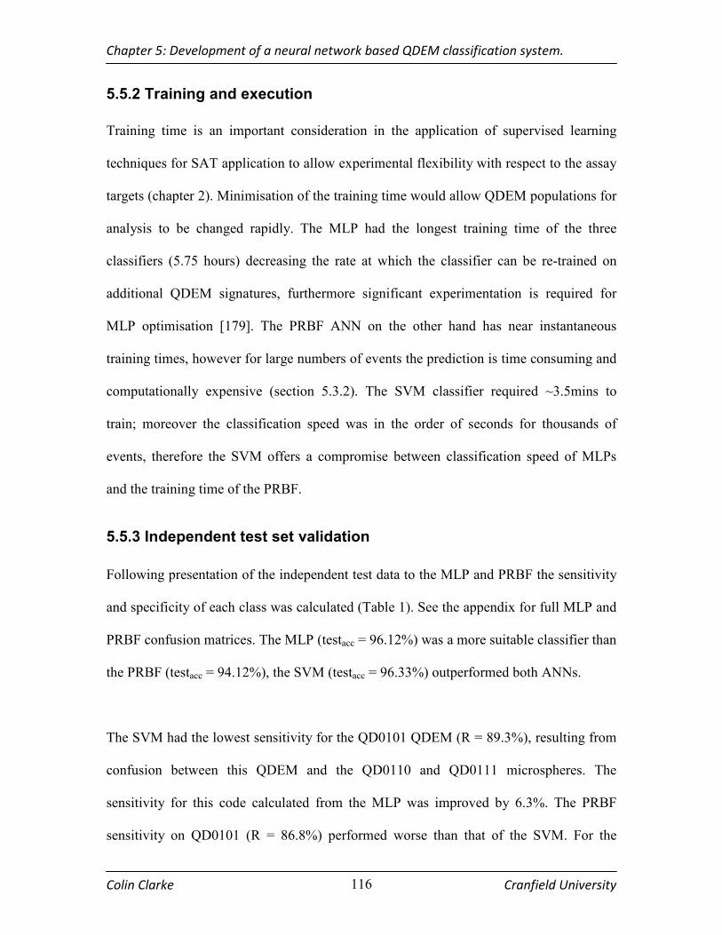
Chapter 5: Development of a neural network based QDEM classification system.
Colin Clarke Cranfield University 116
5.5.2 Training and execution
Training time is an important consideration in the application of supervised learning
techniques for SAT application to allow experimental flexibility with respect to the assay
targets (chapter 2). Minimisation of the training time would allow QDEM populations for
analysis to be changed rapidly. The MLP had the longest training time of the three
classifiers (5.75 hours) decreasing the rate at which the classifier can be re-trained on
additional QDEM signatures, furthermore significant experimentation is required for
MLP optimisation [179]. The PRBF ANN on the other hand has near instantaneous
training times, however for large numbers of events the prediction is time consuming and
computationally expensive (section 5.3.2). The SVM classifier required ~3.5mins to
train; moreover the classification speed was in the order of seconds for thousands of
events, therefore the SVM offers a compromise between classification speed of MLPs
and the training time of the PRBF.
5.5.3 Independent test set validation
Following presentation of the independent test data to the MLP and PRBF the sensitivity
and specificity of each class was calculated (Table 1). See the appendix for full MLP and
PRBF confusion matrices. The MLP (testacc = 96.12%) was a more suitable classifier than
the PRBF (testacc = 94.12%), the SVM (testacc = 96.33%) outperformed both ANNs.
The SVM had the lowest sensitivity for the QD0101 QDEM (R = 89.3%), resulting from
confusion between this QDEM and the QD0110 and QD0111 microspheres. The
sensitivity for this code calculated from the MLP was improved by 6.3%. The PRBF
sensitivity on QD0101 (R = 86.8%) performed worse than that of the SVM. For the

Chapter 5: Development of a neural network based QDEM classification system.
Colin Clarke Cranfield University 117
QD0110 and QD0111 microspheres the identification sensitivity of both ANNs
underperformed in comparison to the SVM, therefore while the MLP increased the
sensitivity on the QD0101(R = 95.60%) signal, there was a decrease with the QD0110(R
= 89.95%) and QD0111(R = 91.73%) in comparison to the SVM. For the remaining
microspheres sensitivities of the SVM were greater than that of the ANNs or the
difference was small. From the results of independent testing the SVM and MLP yielded
a comparable performance on the unseen data; the PRBF was clearly the worst classifier
with sensitivities for the QD1110 microsphere greatly diminished (R = 84.1%). In order
to further separate the SVM and MLP methods the accuracy of each of the mixture test
solutions were compared (section 5.5.5).
Table 14 MLP and PRBF independent test set validation; true positives (#TP), % specificity (S) and
% sensitivity (R) are shown. The class with the lowest sensitivity for the ANNs are highlighted.
5 HLN-MLP PRBF QDEM
#TP S (%) R (%) #TP S (%) R (%)
1 QD0000 245 99.7 92.93 250 99.7 91.1
2 QD0001 193 99.7 92.16 200 99.7 88.9
3 QD0003 236 100 100 236 100 100
4 QD0010 228 99.6 93.49 230 99.0 92.7
5 QD0011 253 99.9 96.25 257 100 94.8
6 QD0100 216 99.9 99.54 221 99.9 97.3
7 QD0101 217 99.6 95.60 239 99.4 86.8
8 QD0110 188 99.5 89.95 197 99.4 85.8
9 QD0111 224 99.7 91.73 222 99.3 92.6
10 QD0202 214 99.7 99.07 215 99.7 98.6
11 QD1000 230 99.9 98.73 234 99.9 97.0
12 QD1001 220 99.9 100 222 100 99.1
13 QD1010 231 99.7 98.00 246 99.7 92.0
14 QD1011 230 99.9 98.70 229 100 99.1
15 QD1100 162 99.7 94.85 166 99.7 92.6
16 QD1101 224 99.9 95.41 229 99.5 93.3
17 QD1110 185 99.7 88.18 194 99.5 84.1
18 QD1111 228 99.7 98.71 230 99.6 97.9
19 QD2100 213 100 100 213 100 100
20 QD2200 227 99.9 99.13 228 99.9 98.7
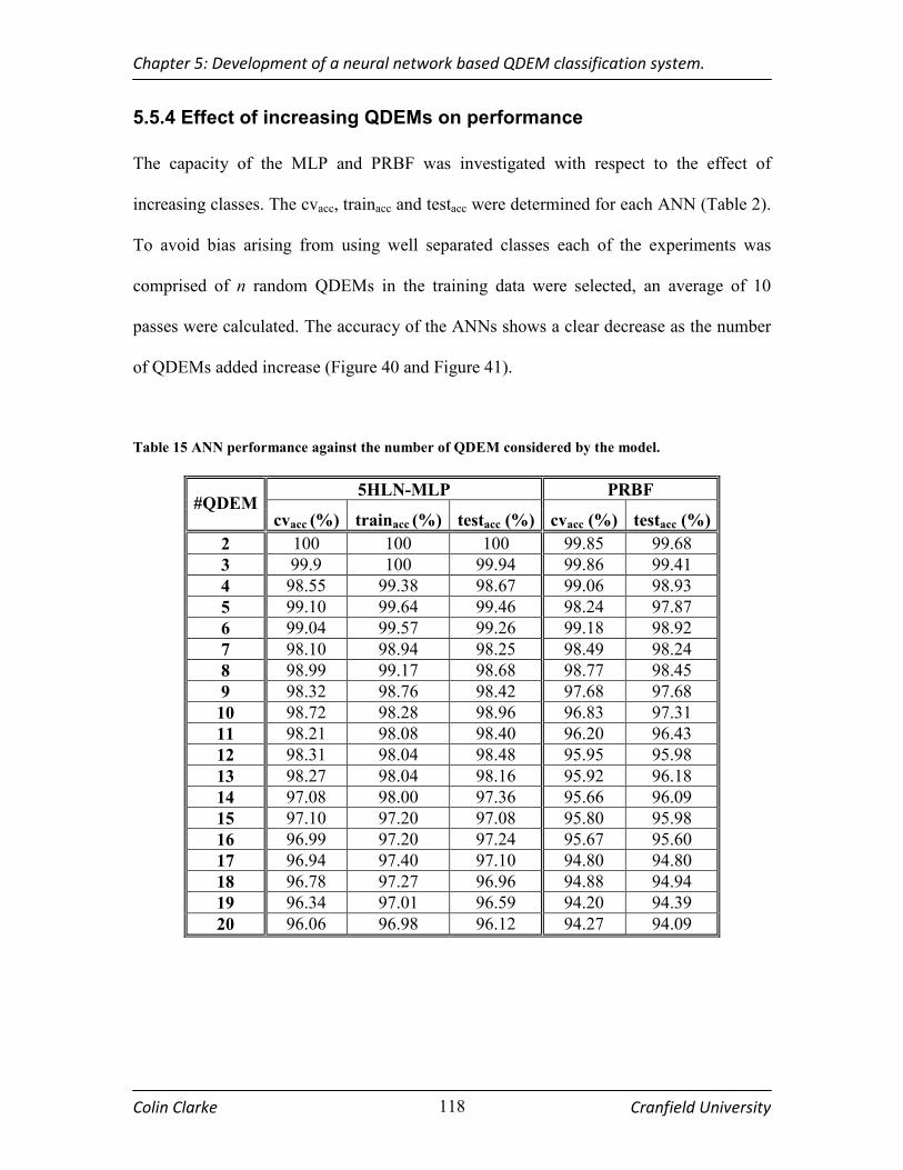
Chapter 5: Development of a neural network based QDEM classification system.
Colin Clarke Cranfield University 118
5.5.4 Effect of increasing QDEMs on performance
The capacity of the MLP and PRBF was investigated with respect to the effect of
increasing classes. The cvacc, trainacc and testacc were determined for each ANN (Table 2).
To avoid bias arising from using well separated classes each of the experiments was
comprised of n random QDEMs in the training data were selected, an average of 10
passes were calculated. The accuracy of the ANNs shows a clear decrease as the number
of QDEMs added increase (Figure 40 and Figure 41).
Table 15 ANN performance against the number of QDEM considered by the model.
5HLN-MLP PRBF #QDEM
cvacc (%) trainacc (%) testacc (%) cvacc (%) testacc (%)
2 100 100 100 99.85 99.68
3 99.9 100 99.94 99.86 99.41
4 98.55 99.38 98.67 99.06 98.93
5 99.10 99.64 99.46 98.24 97.87
6 99.04 99.57 99.26 99.18 98.92
7 98.10 98.94 98.25 98.49 98.24
8 98.99 99.17 98.68 98.77 98.45
9 98.32 98.76 98.42 97.68 97.68
10 98.72 98.28 98.96 96.83 97.31
11 98.21 98.08 98.40 96.20 96.43
12 98.31 98.04 98.48 95.95 95.98
13 98.27 98.04 98.16 95.92 96.18
14 97.08 98.00 97.36 95.66 96.09
15 97.10 97.20 97.08 95.80 95.98
16 96.99 97.20 97.24 95.67 95.60
17 96.94 97.40 97.10 94.80 94.80
18 96.78 97.27 96.96 94.88 94.94
19 96.34 97.01 96.59 94.20 94.39
20 96.06 96.98 96.12 94.27 94.09
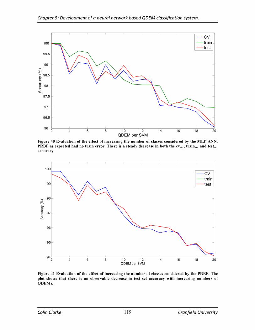
Chapter 5: Development of a neural network based QDEM classification system.
Colin Clarke Cranfield University 119
2 4 6 8 10 12 14 16 18 2096
96.5
97
97.5
98
98.5
99
99.5
100
QDEM per SVM
Accuracy (%)
CV
train
test
Figure 40 Evaluation of the effect of increasing the number of classes considered by the MLP ANN.
PRBF as expected had no train error. There is a steady decrease in both the cvacc, trainacc and testacc
accuracy.
2 4 6 8 10 12 14 16 18 2094
95
96
97
98
99
100
QDEM per SVM
Accuracy (%)
CV
train
test
Figure 41 Evaluation of the effect of increasing the number of classes considered by the PRBF. The
plot shows that there is an observable decrease in test set accuracy with increasing numbers of
QDEMs.
Chapter 5: Development of a neural network based QDEM classification system.
Colin Clarke Cranfield University 120
In the future as additional classes are added to the model, the classification accuracy may
decrease further, possibly as a result of the single net design; The combinatorial binary
classifier of the SVM may offset the decrease in classifier performance. There are
attempts within the community to create more efficient ensemble ANNs through the use
of ECOC schemes which may prove useful for QDEM in the future.
5.5.5 External validation
External validation was carried out using the multiplex solutions for the MLP (Table 16)
and PRBF (Table 17). The MLP incorporates the SOFTMAX function in output layer to
allow probability outputs [196] and classified events below p < 0.5 are filtered, from the
final results, in a similar manner to the SVM. There is no filtering of the classified events
using the PRBF ANN as the network outputs are naturally probability based. Once again
the MC rate and σ2 were determined for each mixture solution as described in section
3.4.2. For the SVM the highest MC rate was for the multiplex tests was 6.4% (test 4). The
performance of the MLP on this test set has decreased by 7.16% in comparison to the
SVM. The FP classifications were mainly observed for the QD0101, QD1010 and
QD1110. For the mixture 1 analysis; the solution containing the most difficult to classify
microspheres performed poorly, with a MC rate of 20.9%, some 16.6% below that of the
SVM. Misclassifications occur mainly with QD0101 and QD1101 microspheres. The
SVM outperformed the MLP or the difference was negligible for the remaining multiplex
testing solutions. The average MLP MC rate from external validation was 6.1%. The
variance of the CCs across the MLP was however poor, again the 7-10 mixtures were
large in comparison to the SVM additionally a higher variance for tests 1-6 was observed.
The average σ2 =56698 for the ten mixtures.

Chapter 5: Development of a neural network based QDEM classification system.
Colin Clarke Cranfield University 121
Table 16 Prediction of unknown events from test samples using MLP ANN classifier. The total
numbers of QDEM classifications (p ≤ 0.5) are shown for each dataset, the microspheres present in
the mixtures are highlighted.
Mixture#
1 2 3 4 5 6 7 8 9 10
QD0000 4 13 0 3 453 41 3 475 278 29
QD0001 1 3 3 5 389 493 8 453 337 585
QD0003 0 0 565 610 0 0 523 0 0 0
QD0010 14 35 3 21 49 63 579 58 58 472
QD0011 551 0 18 6 0 548 0 348 394 450
QD0100 45 538 0 38 457 4 9 352 42 344
QD0101 165 5 2 117 1191 2 848 920 1204 1142
QD0110 331 1 0 330 410 0 4 391 436 376
QD0111 1 0 0 1 60 0 34 92 112 169
QD0202 11 0 219 281 0 18 8 14 27 40
QD1000 0 19 2 37 0 469 508 343 42 403
QD1001 0 0 0 0 0 0 0 0 287 341
QD1010 1 642 0 119 4 587 2 50 111 480
QD1011 2 441 6 302 0 429 2 405 581 460
QD1100 257 252 0 1 106 281 32 107 279 293
QD1101 148 10 3 825 458 599 394 944 844 920
QD1110 388 2 1 54 286 348 321 782 576 549
QD1111 0 1 1 132 0 0 347 50 59 110
QD2100 0 0 682 0 0 0 777 0 0 0
QD
EM
co
de
QD2200 10 6 487 2 10 31 567 20 16 24
#Codes 4 4 4 6 8 8 10 12 12 15
#Events 2000 2000 2000 3000 4000 4000 5000 6000 6000 7500
#Classified 1929 1968 1986 2884 3873 3913 4968 5804 5683 7187
Rejected (%) 3.5 1.6 0.7 3.8 3.1 2.1 0.6 3.2 5.2 4.1
#Correct 1527 1873 3906 2481 3750 3754 4898 5555 5387 7094 CC rate (%) 79.1 95.1 98.3 86.0 96.8 95.9 98.5 95.7 94.7 98.7
σ2 15608 27520 38642 64829 99563 12747 54661 81720 102309 69385
MC rate (%) 20.9 4.9 1.7 14.0 3.2 4.1 1.5 4.3 5.3 1.3
Interestingly the PRBF showed improvement for test 1 (Table 17). The RBF displayed a
MC rate decrease of 11.9%, although there were still 4.7% of events misclassified in
comparison to the SVM. The PRBF performance on mixture 5 was poor, returning 16.7%
misclassified events, 13.7% and 13.5% worse than the SVM and MLP respectively. The
main source of misclassifications in this mixture were due to QD0111 misclassifications
(R = 92.6%). A considerable number of errors were also noted on mixture 4 (12.8%) due

Chapter 5: Development of a neural network based QDEM classification system.
Colin Clarke Cranfield University 122
to significant misclassifications on QD0010 (R = 92.7%) and to lesser extent on QD1110.
The sensitivity of this class was R = 84.11%. The average MC rate for the PBRF external
validation was 7.5%.
Table 17 Prediction of unknown events from test samples using PRBF ANN classifier. (See section
3.4.2 for multiplex test compositions). The QDEMs present in each solution are highlighted.
Mixture #
1 2 3 4 5 6 7 8 9 10
QD0000 8 18 0 4 569 122 8 582 349 73
QD0001 0 1 1 1 298 419 3 374 281 532
QD0003 0 0 562 604 0 0 523 0 0 0
QD0010 47 105 24 234 75 159 1006 150 380 901
QD0011 550 1 28 16 0 551 0 354 396 454
QD0100 24 530 0 22 449 4 16 330 32 317
QD0101 13 1 0 5 429 2 145 285 395 352
QD0110 479 10 0 437 735 2 28 616 686 554
QD0111 27 0 0 28 542 0 717 570 762 871
QD0202 16 2 225 284 0 21 0 17 31 49
QD1000 1 10 3 0 0 446 480 321 0 342
QD1001 0 1 0 0 0 1 0 1 178 215
QD1010 1 508 0 15 3 492 18 13 21 378
QD1011 1 537 1 321 0 496 0 431 624 462
QD1100 176 236 0 8 94 236 9 91 238 217
QD1101 6 2 0 247 225 322 156 331 307 367
QD1110 616 38 0 52 535 671 356 805 703 702
QD1111 35 0 0 722 46 47 222 725 617 707
QD2100 0 0 682 0 0 0 774 0 0 0
QD
EM
co
de
QD2200 0 0 474 0 0 9 539 4 0 7
#Codes 4 4 4 6 8 8 10 12 12 15
#Events 2000 2000 2000 3000 4000 4000 5000 6000 6000 7500
#Correct 1821 1811 1943 2615 3334 3633 4918 5724 5536 7371 CC rate (%) 91.0 90.5 97.1 87.1 83.3 90.8 98.3 95.4 92.2 98.2
σ2 37788 21033 37485 36414 25872 17992 80262 30915 41614 47338
MC rate (%) 9 9.5 2.9 12.8 16.7 9.2 1.6 4.6 7.8 1.8
The average variance for the multiplex tests for the PBRF was σ2 = 37671. An increase is
observed in test 7-10 suggesting that there is an increase in the number of
misclassifications between QDEMs present in the mixture.(For a comparison of the
variances for each of the classifiers see Figure 45)
Chapter 5: Development of a neural network based QDEM classification system.
Colin Clarke Cranfield University 123
The MLP is the most suitable ANN classifier and performs comparably to the SVM in
independent test set validation in terms of accuracy. The SVM however outperforms the
MLP in external validation, moreover the SVM sensitivities for the most difficult to
classify microspheres were superior. Additionally for the SVM there was less variance
exhibited across the ten mixtures, moreover the variance were more uniform.
5.6 Conclusion
The ANNs implemented here have been shown in previous studies to be successful in
classification of events from flow cytometry data. Two ANN implementations, the PRBF
and MLP were trained using the QDEM FCM training set and compared to the
performance of the SVM classifier in chapter 4. Rigorous parameter selection was
applied in order to construct the optimum ANN. For the MLP, a five HLN configuration
yielded the best performance (cvacc = 96.72%, trainacc = 96.95% and test acc = 96.12%). A
PRBF with σ = 2.5 gave the best prediction of the dataset (cvacc = 94.69%, and test acc =
94.38%).The SVM (cvacc = 96.58%, trainacc = 96.72% and testacc = 96.33%) is therefore
the most suitable model for the classification of QDEMs from FCM data. The results of
an external validation using multiplex QDEM test solutions further demonstrated the
suitability of the SVM method. The SVM had a lower MC rate in each of the 10 tests
than both the ANN classifiers and the variance for the SVM CCs (see Figure 45).
Average SVM σ2 = 31479, MLP σ2 = 56698 and PRBF σ2 = 37671.
The accuracy of the SVM is superior for the both the independent test set and multiplex
test sets. Therefore the SVM is the optimum supervised learning technique to classify

Chapter 5: Development of a neural network based QDEM classification system.
Colin Clarke Cranfield University 124
events from the QDEM dataset. The model is highly accurate, sensitive and specific,
outperforming ANNs. It has been shown previously that SVM outperforms the MLP for
classification problems and underperforms with regression, although the differences are
indeed small, the results presented here confirm this.
1 2 3 4 5 6 7 8 9 100
2
4
6
8
10
12
14
16
18
20
22
MC rate (%)
Mixture #
SVM
MLP
PRBF
Figure 42 MC rates of the ten mixture tests for the supervised learning algorithms. The SVM has the
lowest number of misclassifications in each test.
The main difference between the methods relates to model complexity, the MLP network
usually consists of a small number of units in the hidden layer, the SVM incorporates a
much larger number of SVs. The SVM formulation of the learning problem, (i.e.
quadratic optimisation, greatly reduces the number of operations required thus reducing
the training time [197]). The training and execution time of the SVMs were the most
practical. The MLPs training time would prohibit flexibility in the laboratory and the
execution time of PRBF was also time-consuming.

Chapter 6: Overall discussion and conclusions.

Chapter 6: Overall discussion and conclusion
Colin Clarke Cranfield University
126
6.1 Overview
This chapter begins with an overall conclusion of the work described in this thesis. We
begin with a discussion of the classification methods (section 6.2). As part of this project
a user friendly software program was also developed to enable a flow cytometrist to
apply the SVM classifier to QDEM recognition. The main functions of the program are
outlined below (section 6.3). Finally an overall conclusion of this work is presented and
recommendations for future work are outlined (section 6.4 and section 6.5).
6.2 General discussion
Increasing the multiplexing capacity of QDEM libraries to the levels suggested in the
literature (~40,000 unique signatures) requires the utilisation of numerous emission
wavelengths and discrete intensity levels. The first question asked in this thesis was if
current means of QDEM identification were suitable for multicolour QDEMs analysed on
a standard bench top flow cytometer. To this end MPG was evaluated with regard to its
suitability to distinguish members of commercially available QDEMs from FCM data
acquired on an EPICS XL with single laser excitation and four colour detection.
A 20-plex QDEM set was analysed using FCM with approximately 20,000 training
events recorded. An external testing set of QDEM solutions was also prepared and
analysed to provide a benchmark for the methods under examination here, 500 events for
each QDEM in the solution were recorded. While the capacity of the library used was not
large, the coding scheme complexity (4 emission wavelengths and 4 intensity levels) was
greater than those previously described in the literature for QDEMs. The complex coding

Chapter 6: Overall discussion and conclusion
Colin Clarke Cranfield University
127
scheme considered here should give a clear picture of how currently available data
analysis methods would perform at higher levels of multiplexing.
A number of outliers were identified in each QDEM data set possibly arising from
variations in bead manufacture, damage to the bead or variation in measurements. There
is a degree of overspill between the fluorescent channels as the median fluorescent
intensity was not uniform for each detector (Figure 16). The CoeffVs was also high for
the microspheres analysed and provided a suitable dataset to rigorously test the
classification methods.
Investigation of the suitability of a current encoded microsphere identification method
was carried out. The method applied was an expert supervised gating technique, MPG.
MPG in recent times has been applied successfully to such libraries (although the coding
schemes described were less complex than for the QDEMs used here). MPG
misclassified a large proportion of the multiplex solutions showing disappointing levels
of false positive identifications resulting in average MC rate of 9.7% for the 10 mixtures
(14.1% for mixtures 1-6). The most difficult to classify QDEMs in mixture 1 yielded a
MC rate of ~30.6%. As stated previously the results for mixtures 7-10 should be treated
with caution, while the classification accuracy increases, the increasing numbers of
QDEMs in the solution mask the true performance of the model. The variance of correct
classification may show that false positive classifications were present. To this end the
variance of correct classification were calculated. MPG had the highest average variance
across the external validation (Figure 45). The results could not be improved even after
fine tuning of each QDEM region. Moreover multiple classifications were made on single
Chapter 6: Overall discussion and conclusion
Colin Clarke Cranfield University
128
events; due to overlap between the gates (there were more classifications than events in
the testing sets). Therefore the confidence in results obtained using this method was poor.
There was no way to ensure the optimum gate for each population was obtained and the
regions selected were based on the interpretation of the user. Therefore MPG is a
subjective process relying on the skill of a particular user and as the number of QDEMs
per assay increases would the number of plots to be considered increases non-linearly.
MPG was also a time consuming method with ~1 hour required to set and tune the
regions for each population.
The central aim of this thesis was to improve upon the classification accuracy of MPG for
QDEM recognition through the use of supervised learning algorithms. Two of the most
popular supervised algorithms for the discrimination of FCM subpopulations are SVMs
and ANNs. Supervised learning techniques offer a novel solution to QDEM
subpopulation identification. Multivariate machine learning algorithms have advantages
over the MPG in that subjectivity is removed from the process and classification occurs
in a multidimensional space where subtle relationships between detector signals are
considered. SVMs have a good theoretical basis, allowing the multidimensional gating of
subpopulations, moreover through the calculation of the maximal margin hyperplane the
optimum gates can be found. ANN classifiers have also shown good potential FCM
studies, the two most widely used ANN classifiers in the literature were utilised for
QDEM classification A PRBF and MLP ANN were implemented and a comparison with
the MPG and SVM model carried out for the QDEM dataset.

Chapter 6: Overall discussion and conclusion
Colin Clarke Cranfield University
129
An outlier removal procedure was also developed to remove outlying events through
setting an IQR threshold for each parameter, the classification accuracy was improved
using this method. A total of 1,242 events (6.27% of total events acquired) were removed
from the original training data improving the accuracy by 3.31% in the case of the SVM.
As outlier removal was not included as part of the FCSexpress program, outlier filtered
datasets were used only to construct the SVMs and ANNs.
In order to select the optimum model for the data set using SVMs and ANNs, a rigorous
cross validation procedure was carried out for each learning system. An independent
testing set was used to determine the generalisation error of each classifier. The cvacc,
trainacc and testacc of each model (SVM, MLP, and PRBF) are shown below (Table 18).
The classification accuracy of the SVM incorporating a linear kernel and C = 1 using the
OVO multiclass design outperforms those of the ANNs (Table 8) with the best
performance independent test set validation, cvacc = 96.58%, trainacc = 96.72% and testacc =
96.12%.. The MLP is the best ANN for the task. The optimum number of HLNs for the
MLP was determined to be 5 through cross validation; cvacc = 96.72%, trainacc = 96.95%
and testacc = 96.12%. The PRBF ANN (σ = 2.5) had the poorest performance of the three
classifiers cvacc = 94.69% and testacc = 94.38%. The SVM outperforms both ANN
implementations although the difference between the SVM and MLP is small in
independent testing.
Table 18 Comparison of supervised learning techniques for the identification of QDEMs from FCM
data. The best classifier for the QDEM dataset is the SVM.
cvacc (%) trainacc (%) testacc (%)
SVM 96.58 96.72 96.33
MLP 96.72 96.95 96.12
PRBF 94.69 N/A 94.38

Chapter 6: Overall discussion and conclusion
Colin Clarke Cranfield University
130
As a further measure of confidence the sensitivity and specificity for each class was
calculated on the test set predictions. The specificities for the three classifiers were
comparable. The sensitivities for each model are shown below (Figure 43). For the most
difficult microspheres to classify (QD0110, QD0111 and QD0101) the SVM again
yielded the best average performance.
82
84
86
88
90
92
94
96
98
100
QD0000
QD0001
QD0003
QD0010
QD0011
QD0100
QD0101
QD0110
QD0111
QD0202
QD1000
QD1001
QD1010
QD1011
QD1100
QD1101
QD1110
QD1111
QD2100
QD2200
Sensitivity (%)
SVM MLP PRBF
Figure 43 Sensitivities for the three classifiers. See section 4.3.4 for sensitivity calculation. MPG is not
included as there is no independent test set validation.
To test the performance of the classifiers and compare the supervised algorithms with
MPG, 10 QDEM mixtures were prepared using different numbers of QDEMs and
analysed using FCM. The MC rate was calculated as there was no way of independently
verifying the identities of the microspheres from the mixture solutions prior to analysis.
The subpopulations present in the solution were known; hence the false positive results of
each classifier are used to determine suitability.

Chapter 6: Overall discussion and conclusion
Colin Clarke Cranfield University
131
All supervised learning algorithms were shown to return fewer false positives than the
MPG method. The SVM showed excellent classification performance on these samples
clearly outperforming MPG and both ANN methods (Table 19 and Figure 44). The MLP
was the slightly more suitable ANN method outperforming the PRBF method by ~2%.
As stated previously the MC rate results should be treated with caution, as more QDEMs
are included in the mixture. Hence the likely hood of a misclassified event being
designated as QDEM known to be present. In future work it is essential that the
classifications of SAT assay and SVM classification system be run in parallel with a
standard detection platform e.g. microarray.
The variance was also calculated for classifications on QDEMs present in the mixture
solutions (i.e. correct classifications) in each solution for each of the four classifiers
(Figure 45). Calculation of the variance allows a further measure of performance of the
classification techniques. Assuming that each of the testing solutions was homogeneous
(rigorously agitated before aspiration to the flow cytometer), the most suitable classifier
was identified as having the lowest MC rate and the lowest variance between the numbers
of events assigned as correct. Although the QD1100 QDEM seemed to have a diminished
stock concentration each classification paradigm was tested on an identical dataset,
therefore this effect was negated.
Table 19 Comparison of the mixture misclassification rates and CC variances for each of the
classification systems evaluated.
Mixture # MPG SVM MLP PRBF
1-6 14.5 3.9 8.1 10.0 MC rate (%)
All 9.7 2.9 6.1 7.5
1-6 40448 29317 43151 29430 CC variance
(σ2) All 63482 31479 56698 37671

Chapter 6: Overall discussion and conclusion
Colin Clarke Cranfield University
132
1 2 3 4 5 6 7 8 9 100
5
10
15
20
25
30
Mixture #
MC rate (%)
MPG
SVM
MLP
PRBF
Figure 44 Comparison of the MC rate for the 10 multiplex test solutions. The SVM (red) has the
lowest MC rate for all QDEM mixtures (2.9%).
1 2 3 4 5 6 7 8 9 100
2
4
6
8
10
12
14
16x 10
4
Variance (σ2)
Mixture #
MPG
SVM
MLP
PRBF
Figure 45 Variance of each multiplex mixture solution for the four different classification algorithms
used. Assuming a homogenous mixture of QDEMs within the test solutions the variance of the
included QDEMs is used an indicator of classification performance in the external validation. The
SVM (red) demonstrates the lowest variance between the numbers of events detected in each mixture
(average σ2 = 31479).

Chapter 6: Overall discussion and conclusion
Colin Clarke Cranfield University
133
MPG had the highest variance over the mixture solutions (average σ2 = 63482) suggesting
that FPs were present. The SVM (average σ2 = 31479) showed a more balanced
classification of the events expected with a homogeneous, ~50% lower than that of MPG
(average σ2 = 63482). Interestingly the PRBF variance (average σ2 = 37671) was
significantly lower than the MLP (average σ2 = 56698).
The results of independent test set validation and analysis of the QDEMs show the SVM
classifier to be the most suitable for the classification of QDEMs from FCM data
outperforming both MPG and the ANNs. The success of the SVM over the ANN
implementations for this task concurs with Moriss et al. who reported success with SVM
for the discrimination of 20 phytoplankton species. Here a multiclass SVM outperformed
single species RBF ANN and a large optimised RBF ANN for all species [152]. Although
Quinn et al. reported that PRBF had the best performance for the classification of FCM
events during an in vitro viability study, overcoming both the MLP and SVM learning
algorithms [151]. Our work shows that in this case the SVM is superior to that of the
ANNs for classification of QDEMs.
The effect of each of three classifiers when additional microspheres were added was
determined to assess possible scale up issues. However there was no significant
difference observed in the accuracy of each type of model with the addition of QDEMs
for the results here; it is unclear if the classification accuracy would decrease beyond 20
QDEMs. The “scaling up” of RBF ANNs was also deemed to be more problematic for
ANNs in comparison to SVM. The work of Boddy et al. points to SVM handling the
scale of a number of classes to be handled much more efficiently by a SVM [152].

Chapter 6: Overall discussion and conclusion
Colin Clarke Cranfield University
134
2 4 6 8 10 12 14 16 1894
95
96
97
98
99
100
# number of QDEMs
Test accuracy (%)
SVM
MLP
PRBF
Figure 46 Effect of addition of QDEMs considered by the classifier on test set accuracy. The SVM
and MLP decrease at a similar rate, future performance is unknown however the OVO SVM is well
suited to offset these concerns.
The scale-up issue could be a potential limitation of the system although the theory of
OVO SVMs should offset this. The creation of binary classifiers to discriminate against
one another should be dependant on the complexity of the decision boundary required.
Furthermore the performance of the RBF kernel SVM is encouraging, in that the
performance was similar to that of the linear kernel SVM. If the complexity of class
decision boundaries increases, a non-linear SVM could be employed to achieve
classification in a kernel induced feature space e.g. RBF kernel.
Apart from possible scale-up issues, it is not yet clear at this stage if the current
performance of the SVM can be improved. In theory it is possible that the SVM could
exceed 99% accuracy, however accuracy is proportional to the quality of the microsphere
manufacturing and encoding methods therefore increasing the precision of the FCM
analysis (reduction of the CoeffV). Such a reduction in CoeffV may be required for

Chapter 6: Overall discussion and conclusion
Colin Clarke Cranfield University
135
expansion of QDEM libraries. The high throughput nature of FCM also suggests spurious
events are always likely to be present. The use of probability filtering of classification
results removes the majority of these events . While the supervised learning methods
have been shown to be successful perhaps the largest limitation of a supervised learning
system is the application of these methods by laboratory users. The methods described in
chapters 4 and 5 were implemented in the MATLAB environment restricting access to
normal FCM users. To overcome this limitation a user friendly interface was designed in
order to allow rapid and construction and evaluation of multiclass SVMs for the
identification of QDEMs from SVM data. This software program forms a natural
conclusion to the work described in this thesis.
6.3 FlowSVM: A software program for the SVM construction for
the classification of QDEM from FCM data
6.3.1 Introduction
To allow laboratory users to construct and evaluate multiclass SVMs for QDEM
subpopulation identification in flow cytometry a user friendly program, FlowSVM, was
created. FlowSVM is a freely available standalone package developed in the MATLAB
environment allowing standard data plotting and the development and evaluation of SVM
classifiers for QDEM subpopulations. The following sections briefly describe the features
of the program in two parts, firstly the standard data analysis module (section 6.3.2)
allowing traditional FCM plotting and the module for the application of multiclass SVMs
to QDEM classification (section 6.3.3).

Chapter 6: Overall discussion and conclusion
Colin Clarke Cranfield University
136
6.3.2 FlowSVM: FCM data plotting tool
To allow visual inspection of the data prior to SVM training a tool to allow standard
FCM plotting was developed (Figure 47). The FCM data directory must be chosen first,
sample information contained in the HEADER portion of the FCS files is then extracted
and displayed for each file. The FCM data is imported by selecting the relevant file from
the listbox (Figure 47). Note: If the plotting tool is activated directly from the SVM
manager (section 6.3.3), selected FCM data is transferred automatically. There are three
types of plots available, standard non density histograms (univariate, bivariate and
trivariate) and event density plots (scatter, contour and surface). Each FCS in the selected
directory can be overlaid on a single plot with standard histogram plots - a useful feature
for an initial indication of separation between QDEMs. A region selection tool is also
included allowing only events within the selected area to be retained, sample statistics are
recalculated for the selected region and new plots can be drawn. Standard plotting
functions are also included such as 3D plot rotation, magnification, annotation and plot
export.
Figure 47 FlowSVM: Plotting tool interface. A surface plot of event density is shown.
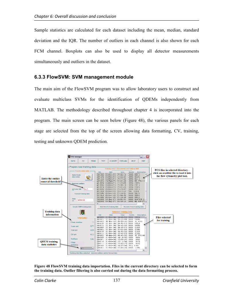
Chapter 6: Overall discussion and conclusion
Colin Clarke Cranfield University
137
Sample statistics are calculated for each dataset including the mean, median, standard
deviation and the IQR. The number of outliers in each channel is also shown for each
FCM channel. Boxplots can also be used to display all detector measurements
simultaneously and outliers in the dataset.
6.3.3 FlowSVM: SVM management module
The main aim of the FlowSVM program was to allow laboratory users to construct and
evaluate multiclass SVMs for the identification of QDEMs independently from
MATLAB. The methodology described throughout chapter 4 is incorporated into the
program. The main screen can be seen below (Figure 48), the various panels for each
stage are selected from the top of the screen allowing data formatting, CV, training,
testing and unknown QDEM prediction.
Figure 48 FlowSVM training data importation. Files in the current directory can be selected to form
the training data. Outlier filtering is also carried out during the data formatting process.

Chapter 6: Overall discussion and conclusion
Colin Clarke Cranfield University
138
The first stage in construction of an SVM for classification is the selection and formatting
of training data. Once a directory has been specified the information contained in the
HEADER is displayed. The user can then select the FCS files containing each class for
SVM training. Selected data files are shown in the lower listbox (double clicking on a file
in the upper listbox activates the plotting tool and transfers the selected training data - see
section 6.3.2). Once data formatting is activated the training data is randomised, split into
the training subsets and written to the LIBSVM format. The IQR cut-off for outlier
removal can also be specified. The training data must be designated file name for data
storage. An individual file is created for each training data subset and the events in each
subset displayed to user along with the number of outliers removed. Standard statistics
for each QDEM population can also be displayed for each class in the training data.
The four phases (parameter selection, training, testing and application) in SVM analysis
are contained in separate panel within the program. Model selection using cross
validation can be carried out by pressing the CV tab. Here the optimum parameters for
the SVM can be determined for the selected cv_set. The four most popular kernels are
implemented and the kernel specific parameters can be assigned. The number of folds
must be entered for the CV procedure. Once the CV has completed the cvacc is outputted
for the selected parameters (Figure 49). If the cvacc is unsatisfactory new parameters can
be re-entered and the process repeated until the optimum model is located.
Following the selection of the optimum parameters SVM training can be carried out in
the TRAIN panel. The training screen is very similar to that of parameter selection. Here

Chapter 6: Overall discussion and conclusion
Colin Clarke Cranfield University
139
the parameters selected through CV can be applied to a training set selected from the data
store. The constructed model is stored for further evaluation.
Figure 49 FlowSVM Parameter selection. CV is carried out on the selected dataset and the results
returned to the user.
Complete independent test set validation of trained SVMs can be carried out in the TEST
panel. The classification accuracy of corresponding testing sets for each model can be
determined. Confusion matrices are also constructed and evaluated automatically and the
sensitivity and specificity of each class outputted to the user. A bar chart of classification
is presented to the user showing the extent of classifications across the test set. Therefore
the user can efficiently determine the success of each SVM model on the data and
maintain a record of each SVM constructed.

Chapter 6: Overall discussion and conclusion
Colin Clarke Cranfield University
140
Validated classifiers can be applied to assay data in the CLASSIFY tab. Here the required
SVM is selected along with the probability cut-off. An FCS file is then selected for
presentation to the SVM. Following classification of the data set a plot of classified
events for each class is displayed. The results of classification and the probability
threshold applied are also recorded for further use.
Figure 50 Prediction of QDEM SAT assays using the FlowSVM program. Trained models are
selected for application to test files. The probability output cutoff points for classification can be
specified and the results stored. A classification plot is presented. The total classifications are
presented to the user.
It is hoped that this tool will make the SVM classifier more accessible to typical
laboratory-based users. Future recommendations for possible extensions of this software
are included in the next section.
Note: The standalone program and source code for the program described above is
freely available on the CD accompanying this thesis.
Chapter 6: Overall discussion and conclusion
Colin Clarke Cranfield University
141
6.4 Overall Conclusion
Suspension array technology has much potential in post genomic applications.
Traditional methods of subpopulation identification methods have been shown to be
limited for the complex encoding strategies possible with nanocyrstal optically encoded
microspheres. An unmodified flow cytometer representative of equipment found in a
variety of locations was used to acquire the QDEM data used in this thesis. Both a
multiparameter gating and unsupervised clustering method were found to be deficient for
the QDEM library analysed in this study. The aim of this work was to improve upon
these methods using supervised learning techniques.
To this end two of the most popular learning paradigms, ANNs and SVMs were applied
to the dataset. A 10-fold cross validation was used to select the optimum classifiers for
each model type. Each model was then evaluated using internal and external validation.
The multiclass SVM classification produced the classifier with the best classification rate
in both independent test set validation (96.33%) and MC rate (2.94%) on the QDEM
mixtures outperforming the ANNs and approaching that of the Luminex system (~2%).
Additionally the training time of the SVM was rapid and classifications could be
performed rapidly an important consideration for FCM. SVMs are well suited to this task
and allowing the optimum gates to be located in a multidimensional space for each class.
There is no reason why organic dye encoded microsphere could not be classified by the
SVM although no such encoding scheme has been considered during this study.

Chapter 6: Overall discussion and conclusion
Colin Clarke Cranfield University
142
A user friendly interface has been created to allow construction and evaluation of SVMs
by laboratory users was developed for flow cytometrists. The program facilitates the
conversion of FCS files into training data, parameter selection, training and independent
test set validation. The resulting SVMs can be applied to unknown FCM in order to
determine the identity of the microspheres present.
It is unclear how the SVM would perform when the encoding scheme is expanded. The
OVO multiclass SVM should classify these microsphere with the similar results as those
presented here, as the design of the classifier only considers any two classes at the same
time. It is therefore likely that the intensity resolution between the encoding levels is the
limiting factor in classification as opposed to the number of colours used or the SVM
paradigm itself.
In conclusion the overall aims of this thesis have been met, an improved classifier for
SAT using QDEM encoded microspheres has been developed using SVMs. SVMs
outperform MPG and ANNs and have potential for the automated identification of
QDEMs in expanded multiplexed assays for applications in genomics and proteomics. It
is hoped that this work will contribute to the application of high throughput SAT assays
using flow cytometry.

Chapter 6: Overall discussion and conclusion
Colin Clarke Cranfield University
143
6.5 Recommendations for future work
While there is no doubt that SVM is a promising classifier for QDEMs, this potential
needs to be built upon. The points below list the areas recommended for future work
• Further SVM evaluation is required at higher levels of multiplexing (increased
numbers of unique QDEMs).
• Application and validation of the SVM QDEM classifier to biological problems, i.e. a
SNP genotyping or gene expression analysis in parallel with microarrays is critical.
• Integration of the hybridisation signal within the SVM or possibly using the reporter
channel as the recording trigger i.e. only hybridised events would be recorded
negating the need for inclusion in the classification algorithm.
• Expansion of the FlowSVM software for increased number of unique microspheres
and the development of a database for storage of experimental parameters, models
and results.
• The integration of the SVM with flow cytometry acquisition software to allow online
classification of events.
• Further development of assay chemistry, including the development of specific
multiplex PCR protocols for applications such as SNP genotyping. Work is currently
under way at Cranfield University toward the development of a multiplex bead assay
for diabetes type II studies.

Bibliography
Colin Clarke Cranfield University
144
Bibliography
1. Lander ES, Linton LM, Birren B, Nusbaum C, Zody MC, Baldwin J, Devon K,
Dewar K, Doyle M, FitzHugh W, et al: Initial sequencing and analysis of the
human genome. Nature 2001, 409:860-921.
2. Venter JC, Adams MD, Myers EW, Li PW, Mural RJ, Sutton GG, Smith HO,
Yandell M, Evans CA, Holt RA, et al: The sequence of the human genome.
Science 2001, 291:1304.
3. Evans WE, Relling MV: Pharmacogenomics: Translating functional genomics
into rational therapeutics. Science 1999, 286:487-491.
4. Veenstra DL, Higashi MK, Phillips KA: Assessing the cost-effectiveness of
pharmacogenomics. Aaps Pharmsci 2000, 2:art. no.-29.
5. Nolan JP, Mandy FF: Suspension array technology: New tools for gene and
protein analysis. Cellular and Molecular Biology 2001, 47:1241-1256.
6. Nolan JP, Sklar LA: Suspension array technology: evolution of the flat-array
paradigm. Trends in Biotechnology 2002, 20:9-12.
7. Dunbar SA: Applications of Luminex (R) xMAP (TM) technology for rapid,
high-throughput multiplexed nucleic acid detection. Clinica Chimica Acta
2006, 363:71-82.
8. Tsuchihashi Z, Dracopoli NC: Progress in high throughput SNP genotyping
methods. The Parmacgenomics journal 2002, 2:103-110.
9. Xu HX, Sha MY, Wong EY, Uphoff J, Xu YH, Treadway JA, Truong A, O'Brien
E, Asquith S, Stubbins M, et al: Multiplexed SNP genotyping using the Qbead
(TM) system: a quantum dot-encoded microsphere-based assay. Nucleic
Acids Research 2003, 31.
10. De Rosa SC, Brenchley JM, Roederer M: Beyond six colors: A new era in flow
cytometry. Nature Medicine 2003, 9:112-117.
11. Wang H-Q, Liu T-C, Cao Y-C, Huang Z-L, Wang J-H, Li X-Q, Zhao Y-D: A
flow cytometric assay technology based on quantum dots-encoded beads.
Analytica Chimica Acta 2006, 580:18-23.

Bibliography
Colin Clarke Cranfield University
145
12. Schena M, Shalon D, Davis RW, Brown DG: Quantitative monitoring of gene
expression patterns with a complementary DNA microarray. Science 1995,
270:467.
13. Hoheisel JD: Microarray technology: beyond transcript profiling and
genotype analysis. Nature Reviews Genetics 2006, 7:200-210.
14. Epstein JR, Biran I, Walt DR: Fluorescence-based nucleic acid detection and
microarrays. Analytica Chimica Acta 2002, 469:3-36.
15. Shepard JRE: Polychromatic microarrays: Simultaneous multicolor array
hybridization of eight samples. Analytical Chemistry 2006, 78:2478-2486.
16. Fulwyler MJ: Method for detecting and separating antigen and antibodies in
blood or other samples. In British patent 1561042. UK; 1976.
17. Horan PK, Wheeless LL: Quantitative Single Cell Analysis and Sorting.
Science 1977, 198:149-157.
18. Fulton RJ, McDade RL, Smith PL, Kienker LJ, Kettman JR: Advanced
multiplexed analysis with the FlowMetrix(TM) system. Clinical Chemistry
1997, 43:1749-1756.
19. Nolan JP, Mandy F: Multiplexed and microparticle-based analyses:
Quantitative tools for the large-scale analysis of biological systems. Cytometry
Part A 2006, 69A:318-325.
20. Fuja T, Hou S, Bryant P: A multiplex microsphere bead assay for comparative
RNA expression analysis using flow cytometry. Journal of Biotechnology 2004,
108:193-205.
21. Henry MR, Stevens PW, Sun J, Kelso DM: Real-time measurements of DNA
hybridization on microparticles with fluorescence resonance energy transfer.
Analytical Biochemistry 1999, 276:204-214.
22. K.E.Meissner EH, R.P.Kruzelock, W.B.Spillman,Jr: Quantum dot-taggd
micropsheres for fluid based DNA microsarrays. physstatso 2003, 0:1355-
1359.
23. Wilson R, Cossins AR, Spiller DG: Encoded microcarriers for high-
throughput multiplexed detection. Angewandte Chemie-International Edition
2006, 45:6104-6117.

Bibliography
Colin Clarke Cranfield University
146
24. Yu JD, Othman MI, Farjo R, Zareparsi S, MacNee SP, Yoshida S, Swaroop A:
Evaluation and optimization of procedures for target labeling and
hybridization of cDNA microarrays. Molecular Vision 2002, 8:130-137.
25. Kellar KL, Iannone MA: Multiplexed microsphere-based flow cytometric
assays. Experimental Hematology 2002, 30:1227-1237.
26. Morgan E, Varro R, Sepulveda H, Ember JA, Apgar J, Wilson J, Lowe L, Chen
R, Shivraj L, Agadir A, et al: Cytometric bead array: a multiplexed assay
platform with applications in various areas of biology. Clinical Immunology
2004, 110:252-266.
27. Tarnok A, Hambsch J, Chen R, Varro R: Cytometric bead array to measure six
cytokines in twenty-five microliters of serum. Clinical Chemistry 2003,
49:1000-1002.
28. Bellisario R, Colinas RJ, Pass KA: Simultaneous measurement of thyroxine
and thyrotropin from newborn dried blood-spot specimens using a
multiplexed fluorescent microsphere immunoassay. Clinical Chemistry 2000,
46:1422-1424.
29. Yan XM, Zhong WW, Tang AJ, Schielke EG, Hang W, Nolan JP: Multiplexed
flow cytometric immunoassay for influenza virus detection and
differentiation. Analytical Chemistry 2005, 77:7673-7678.
30. Fortina P, Kricka LJ, Surrey S, Grodzinski P: Nanobiotechnology: the promise
and reality of new approaches to molecular recognition. Trends in
Biotechnology 2005, 23:168-173.
31. Chan WCW, Nie SM: Quantum dot bioconjugates for ultrasensitive
nonisotopic detection. Science 1998, 281:2016-2018.
32. Alivisatos AP: Semiconductor nanocrystals: New materials through control of
size. Abstracts of Papers of the American Chemical Society 1998, 216:U337-
U337.
33. Ekimov AI, Efros AL, Onushchenko AA: Quantum Size Effect in
Semiconductor Microcrystals. Solid State Communications 1985, 56:921-924.
34. Medintz IL, Uyeda HT, Goldman ER, Mattoussi H: Quantum dot bioconjugates
for imaging, labelling and sensing. Nature Materials 2005, 4:435-446.

Bibliography
Colin Clarke Cranfield University
147
35. Yu WW, Peng XG: Formation of high-quality CdS and other II-VI
semiconductor nanocrystals in noncoordinating solvents: Tunable reactivity
of monomers. Angewandte Chemie-International Edition 2002, 41:2368-2371.
36. Asokan S, Krueger KM, Alkhawaldeh A, Carreon AR, Mu ZZ, Colvin VL,
Mantzaris NV, Wong MS: The use of heat transfer fluids in the synthesis of
high-quality CdSe quantum dots, core/shell quantum dots, and quantum
rods. Nanotechnology 2005, 16:2000-2011.
37. Han MY, Gao XH, Su JZ, Nie S: Quantum-dot-tagged microbeads for
multiplexed optical coding of biomolecules. Nature Biotechnology 2001,
19:631-635.
38. Benecky MJ, Post DR, Schmitt SM, Kochar MS: Detection of hepatitis B
surface antigen in whole blood by coupled particle light scattering
(Copalis(TM)). Clinical Chemistry 1997, 43:1764-1770.
39. Doering WE, Nie SM: Spectroscopic tags using dye-embedded nanoparticies
and surface-enhanced Raman scattering. Analytical Chemistry 2003, 75:6171-
6176.
40. Jin RC, Cao YC, Thaxton CS, Mirkin CA: Glass-bead-based parallel detection
of DNA using composite Raman labels. Small 2006, 2:375-380.
41. Fenniri H, Ding LH, Ribbe AE, Zyrianov Y: Barcoded resins: A new concept
for polymer-supported combinatorial library self-deconvolution. Journal of
the American Chemical Society 2001, 123:8151-8152.
42. Watson DA, Brown LO, Gaskill DF, Naivar M, Graves SW, Doorn SK, Nolan JP:
A flow cytometer for the measurement of Raman spectra. Cytometry Part A
2008, 73A:119-118.
43. Hett JJ: Raman spectroscopy comes to flow cytometry. Cytometry Part A 2008,
73A:109-110.
44. Dejneka MJ, Streltsov A, Pal S, Frutos AG, Powell CL, Yost K, Yuen PK, Muller
U, Lahiri J: Rare earth-doped glass microbarcodes. Proceedings of the
National Academy of Sciences of the United States of America 2003, 100:389-
393.
Bibliography
Colin Clarke Cranfield University
148
45. Walton ID, Norton SM, Balasingham A, He L, Oviso DF, Gupta D, Raju PA,
Natan MJ, Freeman RG: Particles for multiplexed analysis in solution:
Detection and identification of striped metallic particles using optical
microscopy. Analytical Chemistry 2002, 74:2240-2247.
46. Moran EJ, Sarshar S, Cargill JF, Shahbaz MM, Lio A, Mjalli AMM, Armstrong
RW: Radio-Frequency Tag Encoded Combinatorial Library Method for the
Discovery of Tripeptide-Substituted Cinnamic Acid Inhibitors of the Protein-
Tyrosine-Phosphatase Ptp1B. Journal of the American Chemical Society 1995,
117:10787-10788.
47. Amsden B: The production of uniformly sized polymer microspheres.
Pharmaceutical Research 1999, 16:1140-1143.
48. Yi GR, Manoharan VN, Klein S, Brzezinska KR, Pine DJ, Lange FF, Yang SM:
Monodisperse micrometer-scale spherical assemblies of polymer particles.
Advanced Materials 2002, 14:1137-1140.
49. Takeuchi S, Garstecki P, Weibel DB, Whitesides GM: An axisymmetric flow-
focusing microfluidic device. Advanced Materials 2005, 17:1067.
50. Freitas S, Merkle HP, Gander B: Microencapsulation by solvent
extraction/evaporation: reviewing the state of the art of microsphere
preparation process technology. Journal of Controlled Release 2005, 102:313-
332.
51. Martin-Banderas L, Rodriguez-Gil A, Cebolla A, Chavez S, Berdun-Alvarez T,
Garcia JMF, Flores-Mosquera M, Ganan-Calvo AM: Towards high-throughput
production of uniformly encoded microparticles. Advanced Materials 2006,
18:559.
52. O'Brien P, Cummins SS, Darcy D, Dearden A, Masala O, Pickett NL, Ryley S,
Sutherland AJ: Quantum dot-labelled polymer beads by suspension
polymerisation. Chemical Communications 2003:2532-2533.
53. Wang DY, Rogach AL, Caruso F: Semiconductor quantum dot-labeled
microsphere bioconjugates prepared by stepwise self-assembly. Nano Letters
2002, 2:857-861.

Bibliography
Colin Clarke Cranfield University
149
54. Ma Q, Wang XY, Li YB, Shi YH, Su XG: Multicolor quantum dot-encoded
microspheres for the detection of biomolecules. Talanta 2007, 72:1446-1452.
55. Gao XH, Nie SM: Quantum dot-encoded mesoporous beads with high
brightness and uniformity: Rapid readout using flow cytometry. Analytical
Chemistry 2004, 76:2406-2410.
56. Bradley M, Bruno N, Vincent B: Distribution of CdSe quantum dots within
swollen polystyrene microgel particles using confocal microscopy. Langmuir
2005, 21:2750-2753.
57. Cao YC, Huang ZL, Liu TC, Wang HQ, Zhu XX, Wang Z, Zhao YD, Liu MX,
Luo QM: Preparation of silica encapsulated quantum dot encoded beads for
multiplex assay and its properties. Analytical Biochemistry 2006, 351:193-200.
58. Armstrong B, Stewart M, Mazumder A: Suspension arrays for high
throughput, multiplexed single nucleotide polymorphism genotyping.
Cytometry 2000, 40:102-108.
59. Reeve L, Rew DA: New technology in the analytical cell sciences: the laser
scanning cytometer. European Journal of Surgical Oncology 1997, 23:445-450.
60. Darzynkiewicz Z, Bedner E, Li X, Gorczyca W, Melamed MR: Laser-scanning
cytometry: A new instrumentation with many applications. Experimental Cell
Research 1999, 249:1-12.
61. Deptala A, Bedner E, Darzynkiewicz Z: Unique analytical capabilities of laser
scanning cytometry (LSC) that complement flow cytometry. Folia
Histochemica Et Cytobiologica 2001, 39:87-89.
62. Rao RS, Visuri SR, McBride MT, Albala JS, Matthews DL, Coleman MA:
Comparison of multiplexed techniques for detection of bacterial and viral
proteins. Journal of Proteome Research 2004, 3:736-742.
63. Vignali DAA: Multiplexed particle-based flow cytometric assays. Journal of
Immunological Methods 2000, 243:243-255.
64. Braeckmans K, De Smedt SC, Leblans M, Pauwels R, Demeester J: Encoding
microcarriers: Present and future technologies. Nature Reviews Drug
Discovery 2002, 1:447-456.

Bibliography
Colin Clarke Cranfield University
150
65. Pickering JW, Martins TB, Greer RW, Schroder MC, Astill ME, Litwin CM,
Hildreth SW, Hill HR: A multiplexed fluorescent microsphere immunoassay
for antibodies to pneumococcal capsular polysaccharides. American Journal
of Clinical Pathology 2002, 117:589-596.
66. Smith JD, Rose ML: Development of a Luminex based method to detect C4d
binding by HLA antibodies. International Journal of Immunogenetics 2007,
34:290-290.
67. Lowe D, Hathaway M, Briggs D: The high-dose hook effect in the detection
and monitoring of HLA specific antibody by Luminex assay. International
Journal of Immunogenetics 2007, 34:288-288.
68. Powell K, Darke C: ELISA, Luminex (R) and flow cytometry testing of CDC-
defined IgM HLA antibodies. International Journal of Immunogenetics 2007,
34:299-299.
69. Funding M, Hansen TK, Gjedsted J, Ehlers N: Simultaneous quantification of
17 immune mediators in aqueous humour from patients with corneal
rejection. Acta Ophthalmologica Scandinavica 2006, 84:759-765.
70. Hoffmann TK, Sonkoly E, Homey B, Scheckenbach K, Gwosdz C, Bas M,
Chaker A, Schirlau K, Whiteside TL: Aberrant cytokine expression in serum of
patients with adenoid cystic carcinoma and squamous cell carcinoma of the
head and neck. Head and Neck-Journal for the Sciences and Specialties of the
Head and Neck 2007, 29:472-478.
71. Dehqanzada ZA, Storrer CE, Hueman MT, Foley R, Harris K, Jama Y, Shriver
CD, Ponniah S, Peoples GE: Assessing serum cytokine profiles in breast
cancer patients receiving a HER2/neu vaccine using Luminex (R) technology.
Annals of Surgical Oncology 2005, 12:S47-S48.
72. Bobrowski WF, McDuffie JE, Sobocinski G, Chupka J, Olle E, Bowman A,
Albassam M: Comparative methods for multiplex analysis of cytokine protein
expression in plasma of lipopolysaccharide-treated mice. Cytokine 2005,
32:194-198.

Bibliography
Colin Clarke Cranfield University
151
73. Proft T, Schrage B, Fraser JD: The cytokine response to streptococcal
Superantigens varies between individual toxins and between individuals:
Implications for the pathogenesis of group A streptococcal diseases. Journal
of Interferon and Cytokine Research 2007, 27:553-557.
74. Killebrew DA, Shikuma CM, Gerschenson M: Luminex cytokine expression
array in subcutaneous fat adipocytes, preadipocytes and macrophages in
HIV-lipoatrophic patients. Antiviral Therapy 2006, 11:L25-L26.
75. Yurkovetsky ZR, Kirkwood JM, Edington HD, Marrangoni AM, Velikokhatnaya
L, Winans MT, Gorelik E, Lokshin AE: Multiplex analysis of serum cytokines
in melanoma patients treated with interferon-alpha 2b. Clinical Cancer
Research 2007, 13:2422-2428.
76. Schmitt M, Bravo IG, Snijders PJF, Gissmann L, Pawlita M, Waterboer T: Bead-
based multiplex genotyping of human papillomaviruses. Journal of Clinical
Microbiology 2006, 44:504-512.
77. Naciff JM, Richardson BD, Oliver KG, Jump ML, Torontali SM, Juhlin KD, Carr
GJ, Paine JR, Tiesman JA, Daston GP: Design of a microsphere-based high-
throughput gene expression assay to determine estrogenic potential.
Environmental Health Perspectives 2005, 113:1164-1171.
78. Jiang HL, Zhu HH, Zhou LF, Chen F, Chen Z: Genotyping of human
papillomavirus in cervical lesions by L1 consensus PCR and the Luminex
xMAP system. Journal of Medical Microbiology 2006, 55:715-720.
79. Flagella M, Bui S, Zheng Z, Nguyen CT, Zhang AG, Pastor L, Ma YQ, Yang W,
Crawford KL, McMaster GK, et al: A multiplex branched DNA assay for
parallel quantitative gene expression profiling. Analytical Biochemistry 2006,
352:50-60.
80. Deregt D, Gilbert SA, Dudas S, Pasick J, Baxi S, Burton KM, Baxi MK:
Multiplex DNA suspension microarray for simultaneous detection and
differentiation of classical swine fever virus and other pestiviruses. Journal of
Virological Methods 2006, 136:17-23.

Bibliography
Colin Clarke Cranfield University
152
81. Li ZP, Kambara H: Single nucleotide polymorphism analysis based on
minisequencing coupled with a fluorescence microsphere technology. Journal
of Nanoscience and Nanotechnology 2005, 5:1256-1260.
82. Brown JT, Lahey C, Laosinchai-Wolf W, Hadd AG: Polymorphisms in the
glucocerebrosidase gene and pseudogene urge caution in clinical analysis of
Gaucher disease allele c.1448T > C (L444P). Bmc Medical Genetics 2006, 7:-.
83. Nam JM, Thaxton CS, Mirkin CA: Nanoparticle-based bio-bar codes for the
ultrasensitive detection of proteins. Science 2003, 301:1884-1886.
84. Cooper DN, Smith BA, Cooke HJ, Niemann S, Schmidtke J: An Estimate of
Unique DNA-Sequence Heterozygosity in the Human Genome. Human
Genetics 1985, 69:201-205.
85. Hiratsuka M, Sasaki T, Mizugaki M: Genetic testing for pharmacogenetics and
its clinical application in drug therapy. Clinica Chimica Acta 2006, 363:177-
186.
86. Hayashi K, Hashimoto N, Daigen M, Ashikawa I: Development of PCR-based
SNP markers for rice blast resistance genes at the Piz locus. Theoretical and
Applied Genetics 2004, 108:1212-1220.
87. Feltus FA, Wan J, Schulze SR, Estill JC, Jiang N, Paterson AH: An SNP
resource for rice genetics and breeding based on subspecies Indica and
Japonica genome alignments. Genome Research 2004, 14:1812-1819.
88. Chen LM, Perlina A, Lee CJ: Positive selection detection in 40,000 human
immunodeficiency virus (HIV) type 1 sequences automatically identifies drug
resistance and positive fitness mutations in HIV protease and reverse
transcriptase. Journal of Virology 2004, 78:3722-3732.
89. Leeder JS: Pharmacogenetics and pharmacogenomics. Pediatric Clinics of
North America 2001, 48:765-+.
90. Marshall E: Genomics - Drug firms to create public database of genetic
mutations. Science 1999, 284:406-407.
91. Mollevi DG, Serrano T, Ginesta MM, Valls J, Torras J, Navarro M, Ramos E,
Germa JR, Jaurrieta E, Moreno V, et al: Mutations in TP53 are a prognostic

Bibliography
Colin Clarke Cranfield University
153
factor in colorectal hepatic metastases undergoing surgical resection.
Carcinogenesis 2007, 28:1241-1246.
92. Castro MG, Rodriguez-Pascual F, Magan-Marchal N, Reguero JR, Alonso-
Montes C, Moris C, Alvarez V, Lamas S, Coto E: Screening of the endothelin1
gene (EDN1) in a cohort of patients with essential left ventricular
hypertrophy. Annals of Human Genetics 2007, 71:601-610.
93. Yoo NJ, Soung YH, Lee SH, Jeong EG, Lee SH: Mutational analysis of
caspase-14 gene in common carcinomas. Pathology 2007, 39:330-333.
94. Bozzi A, Pereira PPN, Reis BS, Goulart MI, Pereira MCN, Pedroso EP, Leite MF,
Goes AM: Interleukin-10 and tumor necrosis factor-alpha single nucleotide
gene polymorphism frequency in paracoccidioidomycosis. Human
Immunology 2006, 67:931-939.
95. Hammerschmied CG, Stoehr R, Walter B, Wieland WF, Hartmann A, Blaszyk H,
Denzinger S: Role of the STK15 Phe31Ile polymorphism in renal cell
carcinoma. Oncology Reports 2007, 17:3-7.
96. Saiki RK, Walsh PS, Levenson CH, Erlich HA: Genetic-Analysis of Amplified
DNA with Immobilized Sequence-Specific Oligonucleotide Probes.
Proceedings of the National Academy of Sciences of the United States of America
1989, 86:6230-6234.
97. Macdonald SJ, Pastinen T, Genissel A, Cornforth TW, Long AD: A low-cost
open-source SNP genotyping platform for association mapping applications.
Genome Biology 2005, 6.
98. Cai H, White PS, Torney D, Deshpande A, Wang ZL, Marrone B, Nolan JP: Flow
cytometry-based minisequencing: A new platform for high-throughput
single-nucleotide polymorphism scoring. Genomics 2000, 66:135-143.
99. Sundaresan BC, Xu M, Davis-Fleischer K, Phillips M, Bell PA, Boyce-Jacino M:
Bench-top genotyping using a 96 strip-well primer extension SNP-IT (TM)
assay. American Journal of Human Genetics 2001, 69:460-460.
100. Ross P, Hall L, Smirnov I, Haff L: High level multiplex genotyping by MALDI-
TOF mass spectrometry. Nature Biotechnology 1998, 16:1347-1351.

Bibliography
Colin Clarke Cranfield University
154
101. Cronin MT, Frueh F, Pho M, Dutta D, Brennan TM: Applying rapid DNA
microarray optimization capability to SNP screening and genotyping.
American Journal of Human Genetics 1999, 65:A224-a224.
102. Flavell AJ, Bolshakov VN, Booth A, Jing R, Russell J, Ellis THN, Isaac P: A
microarray-based high throughput molecular marker genotyping method:
the tagged microarray marker (TAM) approach. Nucleic Acids Research
2003, 31.
103. Ye F, Li MS, Taylor JD, Nguyen Q, Colton HM, Casey WM, Wagner M, Weiner
MP, Chen JW: Fluorescent microsphere-based readout technology for
multiplexed human single nucleotide polymorphism analysis and bacterial
identification. Human Mutation 2001, 17:305-316.
104. Chen JW, Iannone MA, Li MS, Taylor JD, Rivers P, Nelsen AJ, Slentz-Kesler
KA, Roses A, Weiner MP: A microsphere-based assay for multiplexed single
nucleotide polymorphism analysis using single base chain extension. Genome
Research 2000, 10:549-557.
105. Rockenbauer E, Petersen K, Vogel U, Bolund L, Kolvraa S, Nielsen KV, Nexo
BA: SNP genotyping using microsphere-linked PNA and flow cytometric
detection. Cytometry Part A 2005, 64A:80-86.
106. Deshpande A, Nolan JP, White PS, Valdez YE, Hunt WC, Peyton CL, Wheeler
CM: TNF-alpha promoter polymorphisms and susceptibility to human
papillomavirus 16-associated cervical cancer. Journal of Infectious Diseases
2005, 191:969-976.
107. Yang L, Tran DK, Wang X: BADGE, BeadsArray for the Detection of Gene
Expression, a high-throughput diagnostic bioassay. Genome Research 2001,
11:1888-1898.
108. Eastman PS, Ruan WM, Doctolero M, Nuttall R, De Feo G, Park JS, Chu JSF,
Cooke P, Gray JW, Li S, Chen FQF: Qdot nanobarcodes for multiplexed gene
expression analysis. Nano Letters 2006, 6:1059-1064.
109. Nielsen UB, Geierstanger BH: Multiplexed sandwich assays in microarray
format. Journal of Immunological Methods 2004, 290:107-120.
Bibliography
Colin Clarke Cranfield University
155
110. Carson RT, Vignali DAA: Simultaneous quantitation of 15 cytokines using a
multiplexed flow cytometric assay. Journal of Immunological Methods 1999,
227:41-52.
111. Moss DM, Montgomery JM, Newland SV, Priest JW, Lammie PJ: Detection of
Cryptosporidium antibodies in sera and oral fluids using multiplex bead
assay. Journal of Parasitology 2004, 90:397-404.
112. Mchugh TM, Miner RC, Logan LH, Stites DP: Simultaneous Detection of
Antibodies to Cytomegalo-Virus and Herpes-Simplex Virus by Using Flow-
Cytometry and a Microsphere-Based Fluorescence Immunoassay. Journal of
Clinical Microbiology 1988, 26:1957-1961.
113. Adams EW, Ueberfeld J, Ratner DM, O'Keefe BR, Walt DR, Seeberger PH:
Encoded fiber-optic microsphere arrays for probing protein-carbohydrate
interactions. Angewandte Chemie-International Edition 2003, 42:5317-5320.
114. Chapman GV: Instrumentation for flow cytometry JImmuno meth 2000, 3.
115. Nunez R: Flow Cytometery: Principals and instrumentation. Curr Issues Mol
Biol 2001, 2:39-45.
116. Bogh LDD, T.A. : Flow cytometry instrumentation in research and clinical
laboratories ClinLab Sci 1993, 6:167-173.
117. Lowe MS, A., Zhang,Y.Z., and Getts,R. : Multiplexed, particle-based detection
of DNA using flow cytometry with 3DN dendrimers for signam amplification
Cytometry A 2004, 60:135-144.
118. Mycoy JP, Jr and Carey, J.L. : Recent advances in flow cytometric techniques
for cancer detection and prognosis. ImmunolSer 1990, 53:171-187.
119. Poletav AI, Gnuchev,N.V.,and Zelenin,A.V. : Flow cytometry and cell
sorting:currnet state and prosects for use in molecular biology. 1987, 21:23-
27.
120. Yasa MH, Bektas,A., Yukselen,V., Akbulut,H., Camci,C., and Ormeci,N.: DNA
analysis and DNA ploidy in gastric cancer and gastric precancerous lesions.
International Journal of Clinical Practice 2005, 59:1029-1033.
121. Shapiro HM: Practical flow cytometry. Wiley-Liss; 2003.

Bibliography
Colin Clarke Cranfield University
156
122. Subira D, Gorgolas M, Castanon S, Serrano C, Roman A, Rivas F, Thomas JF:
Advantages of flow cytometry immunophenotyping for the diagnosis of
central nervous system non-Hodgkin's lymphoma in AIDS patients. Hiv
Medicine 2005, 6:21-26.
123. Bertuzzi A, Gandolfi A, Germani A, Spano M, Starace G, Vitelli R: Analysis of
DNA-Synthesis Rate of Cultured-Cells from Flow Cytometric Data.
Cytometry 1984, 5:619-628.
124. Kelley KA, McDowell JL: Practical considerations for the selection and use of
optical filters in flow cytometry. Cytometry 1988, 9:277-280.
125. V.Watson J: Flow Cytomtetry Data Analysis: Basic concepts and statistics.
Cambridge university press; 1992.
126. .
127. Snow C: Flow cytometer electronics. Cytometry Part A 2004, 57A:63-69.
128. Dean PN, Bagwell CB, Lindmo T, Murphy RF, Salzman GC: Introduction to
Flow-Cytometry Data File Standard. Cytometry 1990, 11:321-322.
129. [Anon]: Data File Standard for Flow-Cytometry - Data File Standards
Committee of the Society for Analytical Cytology. Cytometry 1990, 11:323-
332.
130. Herzenberg LA, Tung J, Moore WA, Herzenberg LA, Parks DR: Interpreting
flow cytometry data: a guide for the perplexed. Nature Immunology 2006,
7:681-685.
131. Camilla C, Mely L, Magnan A, Casano B, Prato S, Debono S, Montero F, Defoort
JP, Martin M, Fert V: Flow cytometric microsphere-based immunoassay:
Analysis of secreted ctytokines in whole-blood samples from asthmatics.
Clinical and Diagnostic Laboratory Immunology 2001, 8:776-784.
132. Keij JF, Steinkamp JA: Flow cytometric characterization and classification of
multiple dual-color fluorescent microspheres using fluorescence lifetime.
Cytometry 1998, 33:318-323.
133. Yao G, Wang L, Wu YR, Smith J, Xu JS, Zhao WJ, Lee EJ, Tan WH: FloDots:
luminescent nanoparticles. Analytical and Bioanalytical Chemistry 2006,
385:518-524.

Bibliography
Colin Clarke Cranfield University
157
134. Bhaskar H, Hoyle DC, Singh S: Machine learning in bioinformatics: A brief
survey and recommendations for practitioners. Computers in Biology and
Medicine 2006, 36:1104-1125.
135. Harz M, Rosch P, Peschke KD, Ronneberger O, Burkhardt H, Popp J: Micro-
Raman spectroscopic identification of bacterial cells of the genus
Staphylococcus and dependence on their cultivation conditions. Analyst 2005,
130:1543-1550.
136. Christianini NS-T, John; : An Introduction to Support Vector Machines and Other
Kernel-based Learning Methods. Cambridge Universtiy Press; 2000.
137. Vladimir NV: The nature of statistical learning theory. Springer-Verlag New
York, Inc.; 1995.
138. Burges C: A Tutorial on Support Vector Machines for Pattern Recognition.
Data Mining and Knowledge Discovery 1998, 2:121-167.
139. Minsky ML, Papert SA: Perceptrons. Expanded Edition 1990 edn: MIT Press;
1969.
140. Bredensteiner EJ, Bennett KP: Multicategory classification by support vector
machines. Computational Optimization and Applications 1999, 12:53-79.
141. Weston J, Watkins C: Multi-class support vector machines. Technical Report
CSD-TR-98-04 , Royal Holloway, University of London, 1998.
142. Tsujinishi D, Abe S: Fuzzy least squares support vector machines for
multiclass problems. Neural Networks 2003, 16:785-792.
143. ???: Multiclass support vector machines. 2008.
144. Hastie T, Tibshirani R: Classification by pairwise coupling. Annals of Statistics
1998, 26:451-471.
145. Hsu CW, Lin CJ: A comparison of methods for multiclass support vector
machines. Ieee Transactions on Neural Networks 2002, 13:415-425.
146. Lin CHaCLHaC: A comparison of methods for multi-class support vector
machines. 2001.
147. Melgani F, Bruzzone L: Classification of hyperspectral remote sensing images
with support vector machines. Ieee Transactions on Geoscience and Remote
Sensing 2004, 42:1778-1790.

Bibliography
Colin Clarke Cranfield University
158
148. Liu Y, Zheng YF: One-against-all multi-class SVM classification using
reliability measures. In IEEE International Joint Conference on Neural
Networks; 31/08/05. 2005: 849-854.
149. Cualing HD: Automated analysis in flow cytometry. Cytometry 2000, 42:110-
113.
150. Adjouadi M, Zong N, Ayala M: Multidimensional pattern recognition and
classification of white blood cells using support vector machines. Particle &
Particle Systems Characterization 2005, 22:107-118.
151. Quinn J, Fisher PW, Capocasale RJ, Achuthanandam R, Kam M, Bugelski PJ,
Hrebien L: A statistical pattern recognition approach for determining cellular
viability and lineage phenotype in cultured cells and murine bone marrow.
Cytometry Part A 2007, 71A:612-624.
152. Morris CW, Autret A, Boddy L: Support vector machines for identifying
organisms - a comparison with strongly partitioned radial basis function
networks. Ecological Modelling 2001, 146:57-67.
153. Toedling J, Rhein P, Ratei R, Karawajew L, Spang R: Automated in-silico
detection of cell populations in flow cytometry readouts and its application to
leukemia disease monitoring. Bmc Bioinformatics 2006, 7:-.
154. J.Tukey: Exploratory Data Analysis. Addison-Wesely; 1977.
155. Lin C-CCaC-J: LIBSVM: a library for support vector machines.
156. Ting-Fan W, Chih-Jen L, Ruby CW: Probability Estimates for Multi-class
Classification by Pairwise Coupling. J Mach Learn Res 2004, 5:975-1005.
157. Breiman L: Heuristics of instability and stabilization in model selection.
Annals of Statistics 1996, 24:2350-2383.
158. Goutte C: Note on free lunches and cross-validation. Neural Computation 1997,
9:1245-1249.
159. Frank RE, Massy WF, Morrison DG: Bias in multiple discriminate analysis.
Journal of Marketing Research 1965, 2:250-258.
160. Rocco SCM, Moreno JA: System reliability evaluation using Monte Carlo &
support vector machine. Annual Reliability and Maintainability Symposium,
2003 Proceedings 2003:482-486.

Bibliography
Colin Clarke Cranfield University
159
161. Hua SJ, Sun ZR: Support vector machine approach for protein subcellular
localization prediction. Bioinformatics 2001, 17:721-728.
162. Keerthi SS, Lin CJ: Asymptotic behaviors of support vector machines with
Gaussian kernel. Neural Computation 2003, 15:1667-1689.
163. Winters-Hilt S, Yelundur A, McChesney C, Landry M: Support Vector Machine
implementations for classification & clustering. Bmc Bioinformatics 2006, 7:-.
164. Mayoraz E, Alpaydin E: Support vector machines for multi-class
classification. Engineering Applications of Bio-Inspired Artificial Neural
Networks, Vol Ii 1999, 1607:833-842.
165. Coporation L: Luminex 200 specifications. 2005.
166. Aleksander I: The Handbook of Brain Theory and Neural Networks -
Arbib,Ma. Nature 1995, 376:564-564.
167. Jain AK, Mao JC, Mohiuddin KM: Artificial neural networks: A tutorial.
Computer 1996, 29:31-&.
168. Mcculloch WS, Pitts W: A Logical Calculus of the Ideas Immanent in Nervous
Activity (Reprinted from Bulletin of Mathematical Biophysics, Vol 5, Pg 115-
133, 1943). Bulletin of Mathematical Biology 1990, 52:99-115.
169. Rosenblatt F: The Perceptron - a Probabilistic Model for Information-Storage
and Organization in the Brain. Psychological Review 1958, 65:386-408.
170. Hopfield JJ: Neural Networks and Physical Systems with Emergent Collective
Computational Abilities. Proceedings of the National Academy of Sciences of
the United States of America-Biological Sciences 1982, 79:2554-2558.
171. Werbos PJ: Generalization of Backpropagation with Application to a
Recurrent Gas Market Model. Neural Networks 1988, 1:339-356.
172. Yao X, Liu Y: Neural Networks for Breast Cancer Diagnosis. Proceedings of
the 1999 Congress on Evolutionary Computation 1999, 3:1767.
173. Somervuo P, Kohonen T: Self-organizing maps and learning vector
quantization for feature sequences. Neural Processing Letters 1999, 10:151-
159.
Bibliography
Colin Clarke Cranfield University
160
174. Boddy L, Morris CW, Wilkins MF, Tarran GA, Burkill PH: Neural-Network
Analysis of Flow Cytometric Data for 40 Marine-Phytoplankton Species.
Cytometry 1994, 15:283-293.
175. Jonker R, Groben R, Tarran G, Medlin L, Wilkins M, Garcia L, Zabala L, Boddy
L: Automated identification and characterisation of microbial populations
using flow cytometry: the AIMS project. Scientia Marina 2000, 64:225-234.
176. Wilkins MF, Boddy L, Morris CW, Jonker RR: Identification of phytoplankton
from flow cytometry data by using radial basis function neural networks.
Applied and Environmental Microbiology 1999, 65:4404-4410.
177. Smits JRM, Breedveld LW, Derksen MWJ, Kateman G, Balfoort HW, Snoek J,
Hofstraat JW: Pattern-Classification with Artificial Neural Networks -
Classification of Algae, Based Upon Flow Cytometer Data. Analytica Chimica
Acta 1992, 258:11-25.
178. Morris CW, Boddy L, Allman R: Identification of Basidiomycete Spores by
Neural Network Analysis of Flow-Cytometry Data. Mycological Research
1992, 96:697-701.
179. Boddy L, Wilkins MF, Morris CW: Pattern recognition in flow cytometry.
Cytometry 2001, 44:195-209.
180. Kothari R, Cualing H, Balachander T: Neural network analysis of flow
cytometry immunophenotype data. Ieee Transactions on Biomedical
Engineering 1996, 43:803-810.
181. Ravdin PM, Clark GM, Hough JJ, Owens MA, Mcguire WL: Neural Network
Analysis of DNA Flow-Cytometry Histograms. Cytometry 1993, 14:74-80.
182. Haykin S: Neural Networks A Comprehensive Foundation Prentice-Hall; 1998.
183. Hassoun MH: Fundamentals of artificial neural networks. MIT Press; 1995.
184. Rumelhart DE, Hinton GE, Williams RJ: Learning Representations by Back-
Propagating Errors. Nature 1986, 323:533-536.
185. Sejnowski TJ, Kienker PK, Hinton GE: Learning Symmetry Groups with
Hidden Units - Beyond the Perceptron. Physica D 1986, 22:260-275.
186. Broomhead DS, D L: Multivariate functional interpolation and adaptive
networks. Complex System 2, 1988:321-355.

Bibliography
Colin Clarke Cranfield University
161
187. Tipping ME, Lowe D: Shadow targets: A novel algorithm for topographic
projections by radial basis functions. Neurocomputing 1998, 19:211-222.
188. Roy A, Govil S, Miranda R: An Algorithm to Generate Radial Basis Function
(Rbf)-Like Nets for Classification Problems. Neural Networks 1995, 8:179-
201.
189. Moody J, Darken C: Fast learning in networks of locally tuned processing
units. Nueral Computation 1989, 1:281-294.
190. Musavi MT, Ahmed W, Chan KH, Faris KB, Hummels DM: On the Training of
Radial Basis Function Classifiers. Neural Networks 1992, 5:595-603.
191. Blue JL, Candela GT, Grother PJ, Chellappa R, Wilson CL: Evaluation of
Pattern Classifiers for Fingerprint and Ocr Applications. Pattern Recognition
1994, 27:485-501.
192. Wasserman PD: Advanced Methods in Neural Computing. New York: Van
Nostrand Reinhold; 1993.
193. Denmark TUo: ANN:DTU Toolbox. 2002.
194. Hintz-Madsen M, Hansen LK, Larsen J, Pedersen MW, Larsen M: Neural
classifier construction using regularization, pruning and test error
estimation. Neural Networks 1998, 11:1659-1670.
195. MathWorks: MATLAB: User Manual 7.3.
196. Arribas JI, Cid-Sueiro J: A model selection algorithm for a Posteriori
probability estimation with neural networks. Ieee Transactions on Neural
Networks 2005, 16:799-809.
197. Osowski S, Siwek K, Markiewicz T: MLP and SVM networks - a comparative
study. In 6th Nordic Signal Processing Symposium; Espoo, Finland. 2004
198. Roederer M, Hardy RR: Frequency difference gating: A multivariate method
for identifying subsets that differ between samples. Cytometry 2002:134-135.
199. Mario Roederer WM, Adam Treister, Richard R. Hardy, and Leonore A.
Herzenberg Probability Binning Comparison: A metric for Quantitating
Multivariate Distribution Differences Cytometry 2001, 45:47-55.
200. Roederer M, Hardy RR: Frequency difference gating: A multivariate method
for identifying subsets that differ between samples. Cytometry 2001, 45:56-64.

Appendix 1: Frequency difference gating and probability
binning.

Appendix 1: Frequency difference gating and probability difference gating
Colin Clarke Cranfield University
163
Clustering algorithms can be used to identify subsets of cells in FCM data based on
different characteristics of that data. The second standard classification method evaluated
for the QDEM library was an unsupervised clustering method called frequency difference
gating first described by Roeder et al [198]. The technique has overcome previous
limitations including the computational expense of such algorithms and integration of
domain specific knowledge and is implemented as part of the Flojo software suite (Tree
Star, San Carlos, CA). A possible advantage of this method is that no training data is
required for subpopulation identification. Decisions are based solely on the multiplexing
test set distributions and no underlying assumptions are made. The similarity and
dissimilarity of samples can be identified and the data can be gated on events in one
sample that are different from a control even if the differences are not visible on bivariate
plots. A variation of the chi-squared statistic was extended to a multivariate space. The
normalised chi-squared value for the ith bin is calculated as:
( )( )
2#
2
1
'
n nbins
i i
n ni i i
c s
c sχ
=
−=
+∑
n ii c
cc
E= and
n ii s
ss
E=
(3.1)
Where ic and is are the number of control and test samples falling into bin i. cE and
sE are the total events in the control and test samples. In the case of samples where no
control is possible or logical (in our case), the control is the combination of the test
sample events. Each sample is then compared to the combined test control. The algorithm
has been successfully applied to the differentiation of HIV+ and HIV- samples and
mouse B cells [199].
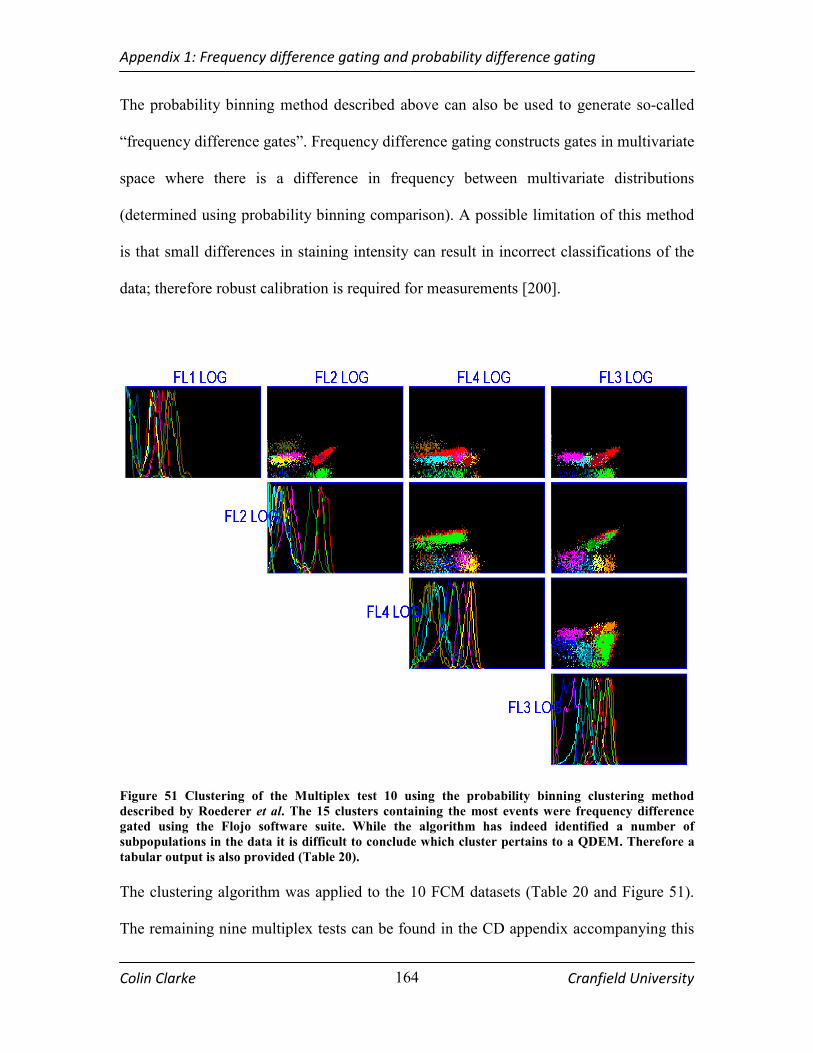
Appendix 1: Frequency difference gating and probability difference gating
Colin Clarke Cranfield University
164
The probability binning method described above can also be used to generate so-called
“frequency difference gates”. Frequency difference gating constructs gates in multivariate
space where there is a difference in frequency between multivariate distributions
(determined using probability binning comparison). A possible limitation of this method
is that small differences in staining intensity can result in incorrect classifications of the
data; therefore robust calibration is required for measurements [200].
Figure 51 Clustering of the Multiplex test 10 using the probability binning clustering method
described by Roederer et al. The 15 clusters containing the most events were frequency difference
gated using the Flojo software suite. While the algorithm has indeed identified a number of
subpopulations in the data it is difficult to conclude which cluster pertains to a QDEM. Therefore a
tabular output is also provided (Table 20).
The clustering algorithm was applied to the 10 FCM datasets (Table 20 and Figure 51).
The remaining nine multiplex tests can be found in the CD appendix accompanying this

Appendix 1: Frequency difference gating and probability difference gating
Colin Clarke Cranfield University
165
thesis. As can be seen from the multiplex results (test 10) it is difficult to reliably assign
identity to the QDEM subpopulations. For the 15 clusters containing the most events, the
biggest cluster contains more than 1900 events while the lowest cluster contains only 93
events. We would expect there to be a greater balance between microsphere classes (as
equal amounts of the stock solution were added to each multiplex solution). It is possible
that more events were acquired for certain QDEM classes however this imbalance in
class detection was not observed during the MPG analysis.
Table 20 Flojo clustering results. The test solutions were clustered using probability binning
comparison and frequency difference gating applied. The results for multiplex test 10 are shown. The
top 15 cluster designations were also plotted (Figure 51). It is difficult from these results to identify
the QDEMs correctly. The output of the Flojo algorithm was deemed to be unsuitable for the
discrimination of the QDEMs from FCM data.
Events Name FL1 FL2 FL3 FL4 QDEM
7500 Parent
1901 Cluster 1 + ++ ++ + 1221
1897 Cluster 2 — + + + 0111
565 Cluster 3 — — — + 0001
493 Cluster 4 — — ++ ++ 0022
405 Cluster 5 + — + — 1010
383 Cluster 6 + — — + 1001
248 Cluster 7 + — + ++ 1012
238 Cluster 8 — — + ++ 0012
228 Cluster 9 — + + — 0110
215 Cluster 10 — — + + 0011
160 Cluster 11 + — — — 1000
123 Cluster 12 — — + — 0010
111 Cluster 13 + + + — 1110
99 Cluster 14 + — — — 1000
93 Cluster 15 + — — — 1000
The second deficiency of the method is that the actual identification of the class is
subjective. Shown above is the output of the analysis, here the fluorescent parameters are
shown where a ranking scheme is used to define the parameters that distinguish the
microspheres (Table 20). It can be seen that the identification of the microspheres

Appendix 1: Frequency difference gating and probability difference gating
Colin Clarke Cranfield University
166
becomes subjective relying on the cluster plot and the user interpretation of the results
shown below.
This point is outlined by Roderer et al. who state that frequency difference gating is
meant to identify subsets in multidimensional space. Confident identification of multiple
populations using this method was impossible. It is likely that this algorithm works best
when a control population is provided. The paper describing this algorithm presented an
example of HIV analysis where a test was provided with excellent results. In our case as
mentioned above a control” set is not applicable. Therefore the Flojo clustering method,
while having a distinct advantage (in that no training set is required) is not suitable for the
identification of QDEMs from the datasets provided. It is expected that by increasing the
number of unique microspheres that the performance of the algorithm would decrease.
In conclusion, each of the ten QDEM mixtures were analysed using this method, however
results were poor. It was difficult to determine the identity of each cluster; moreover
there was a large discrepancy between the numbers of events in each cluster when
compared to the quantities inputted in each QDEM solution. As each QDEM solution
was added to the test solution in equal concentration (except for QD1100) the results
obtained highlight the deficiency of this method for classification of the QDEMs within
the test solutions. Therefore the MPG results provided the benchmark for current QDEM
identification techniques.

Appendix 2: Confusion Matrices.
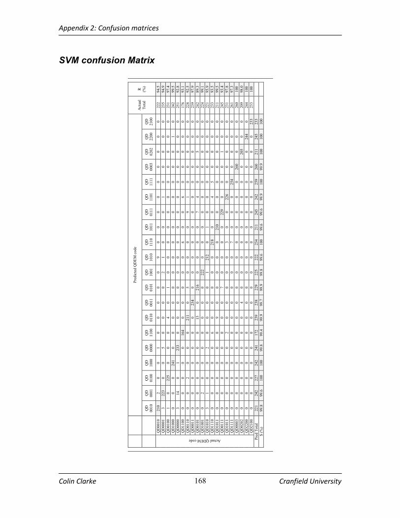
Appendix 2: Confusion matrices
Colin Clarke Cranfield University
168
SVM confusion Matrix
Pre
dic
ted Q
DE
M c
ode
QD
001
0
QD
00
01
QD
0
100
QD
1
000
QD
0
000
Q
D
110
0
QD
011
0
QD
001
1
QD
01
01
QD
1
001
QD
1
010
QD
1110
Q
D
101
1
QD
011
1
QD
110
1
QD
11
11
QD
0
003
QD
0
202
QD
2200
Q
D
210
0
Act
ual
T
ota
l R
(%
)
QD
001
0
21
0
2
0
0
1
0
0
0
0
0
9
0
0
0
0
0
0
0
0
0
22
2
94.5
QD
000
1
3
223
0
0
5
0
0
0
0
2
1
0
0
0
1
0
0
0
0
0
23
5
94.9
QD
010
0
1
0
225
0
0
0
4
0
1
0
0
0
0
0
0
0
0
0
0
0
23
1
97.4
QD
100
0
0
0
0
241
0
0
0
0
0
0
0
0
0
0
0
0
0
0
1
0
24
2
99.5
QD
000
0
3
14
0
1
233
0
0
0
0
0
0
0
0
0
0
0
0
0
0
0
25
1
92.8
QD
110
0
0
0
0
0
0
164
0
0
0
0
0
6
0
0
6
0
0
0
0
0
17
6
93.1
QD
011
0
0
0
2
0
0
0
211
0
5
0
0
0
0
9
1
0
0
0
0
0
22
8
92.5
QD
001
1
0
0
0
0
0
0
0
23
4
0
0
0
0
0
0
0
0
0
0
0
0
23
9
97.9
QD
010
1
0
0
0
0
0
0
15
0
2
16
0
0
0
0
7
4
0
0
5
0
0
24
2
89.3
QD
100
1
0
2
0
0
0
0
0
0
0
222
0
0
0
0
0
0
0
0
0
0
22
4
99.1
QD
101
0
3
1
0
0
2
0
0
0
0
1
212
0
1
0
0
0
0
0
0
0
22
1
95.9
QD
111
0
0
0
0
0
0
6
0
0
0
0
0
218
0
0
4
5
0
0
0
0
23
3
93.5
QD
101
1
0
0
0
0
0
0
9
0
0
0
0
0
210
0
0
0
0
0
0
0
21
1
99.5
QD
011
1
0
0
0
0
0
0
0
0
7
0
0
0
0
229
0
0
0
1
0
0
24
5
93.4
QD
101
1
0
0
0
0
0
2
0
0
0
0
0
3
0
0
22
6
0
0
0
0
0
23
1
97.8
QD
111
1
0
0
0
0
0
0
0
0
0
0
0
7
0
0
0
254
0
0
0
0
26
1
97.3
QD
000
3
0
0
0
0
0
0
0
0
0
0
0
0
0
0
0
0
260
0
0
0
26
0
100
QD
020
2
0
0
0
0
0
0
0
4
0
0
0
0
0
0
0
0
0
205
0
0
20
9
98.0
QD
220
0
0
0
0
0
0
0
0
0
0
0
0
0
0
0
0
0
0
0
244
0
24
4
100
Actual QDEM code
QD
210
0
0
0
0
0
0
0
0
0
0
0
0
0
0
0
0
0
0
0
0
233
23
3
100
Pre
d T
ota
l 22
1
242
227
242
241
172
239
23
8
229
225
222
234
211
245
24
2
259
260
211
245
233
S (
%)
99
.8
99
.6
100
100
99.8
99.4
99.9
99
.7
99
.9
99.8
9
9.6
100
99.6
99.6
99
.9
100
99.9
1
00
100
100
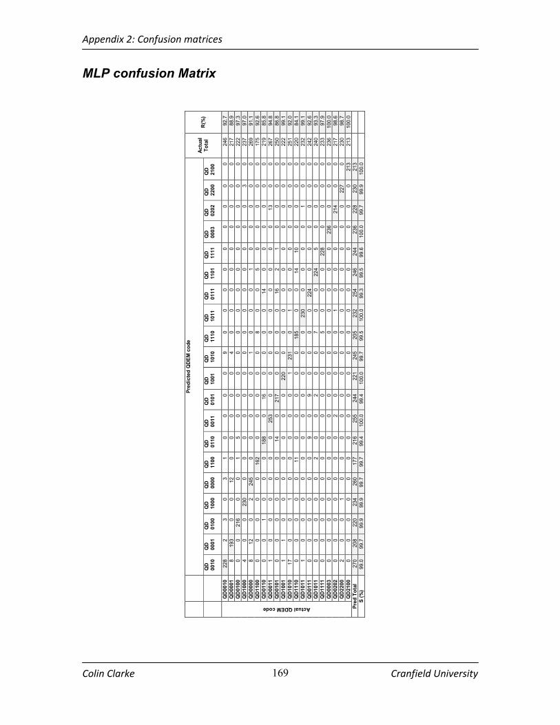
Appendix 2: Confusion matrices
Colin Clarke Cranfield University
169
MLP confusion Matrix
Predicted QDEM code
QD
0010
QD
0001
QD
0100
QD
1000
QD
0000
QD
1100
QD
0110
QD
0011
QD
0101
QD
1001
QD
1010
QD
1110
QD
1011
QD
0111
QD
1101
QD
1111
QD
0003
QD
0202
QD
2200
QD
2100
Actual
Total
R(%
)
QD0010
228
2
3
0
3
1
0
0
0
0
9
0
0
0
0
0
0
0
0
0
246
92.7
QD0001
8
193
0
0
12
0
0
0
0
0
4
0
0
0
0
0
0
0
0
0
217
88.9
QD0100
0
0
216
0
0
1
5
0
0
0
0
0
0
0
0
0
0
0
0
0
222
97.3
QD1000
4
0
0
230
0
0
0
0
0
0
0
0
0
0
0
0
0
0
3
0
237
97.0
QD0000
8
12
0
2
245
0
0
0
0
0
1
0
0
0
1
0
0
0
0
0
269
91.1
QD1100
0
0
0
0
0
162
0
0
0
0
0
8
0
0
5
0
0
0
0
0
175
92.6
QD0110
0
0
1
0
0
0
188
0
16
0
0
0
0
14
0
0
0
0
0
0
219
85.8
QD0011
1
0
0
0
0
0
0
253
0
0
0
0
0
0
0
0
0
13
0
0
267
94.8
QD0101
0
0
0
0
0
0
14
0
217
0
0
0
0
16
2
1
0
0
0
0
250
86.8
QD1001
1
1
0
0
0
0
0
0
0
220
0
0
0
0
0
0
0
0
0
0
222
99.1
QD1010
17
0
0
1
0
0
0
0
0
1
231
0
1
0
0
0
0
0
0
0
251
92.0
QD1110
0
0
0
0
0
11
0
0
0
0
0
185
0
0
14
10
0
0
0
0
220
84.1
QD1011
1
0
0
0
0
0
0
0
0
0
0
0
230
0
0
0
0
1
0
0
232
99.1
QD0111
0
0
0
0
0
0
9
0
9
0
0
0
0
224
0
0
0
0
0
0
242
92.6
QD1011
0
0
0
0
0
2
0
0
2
0
0
7
0
0
224
5
0
0
0
0
240
93.3
QD1111
0
0
0
0
0
0
0
0
0
0
0
5
0
0
0
228
0
0
0
0
233
97.9
QD0003
0
0
0
0
0
0
0
0
0
0
0
0
0
0
0
0
236
0
0
0
236
100.0
QD0202
0
0
0
0
0
0
0
2
0
0
0
0
1
0
0
0
0
214
0
0
217
98.6
QD2200
2
0
0
1
0
0
0
0
0
0
0
0
0
0
0
0
0
0
227
0
230
98.7
Actual QDEM code
QD2100
0
0
0
0
0
0
0
0
0
0
0
0
0
0
0
0
0
0
0
213
213
100.0
Pred Total
270
208
220
234
260
177
216
255
244
221
245
205
232
254
246
244
236
228
230
213
S (%)
99.0
99.7
99.9
99.9
99.7
99.7
99.4
100.0
99.4
100.0
99.7
99.5
100.0
99.3
99.5
99.6
100.0
99.7
99.9
100.0

Appendix 2: Confusion matrices
Colin Clarke Cranfield University
170
PRBF confusion Matrix
Predicted QDEM code
QD
0010
QD
0001
QD
0100
QD
1000
QD
0000
QD
1100
QD
0110
QD
0011
QD
0101
QD
1001
QD
1010
QD
1110
QD
1011
QD
0111
QD
1101
QD
1111
QD
0003
QD
0202
QD
2200
QD
2100
Actual
Total
R(%
)
QD0010
230
2
2
0
3
1
0
0
0
0
8
0
0
0
0
0
0
0
0
0
246
93.49
QD0001
6
200
0
0
9
0
0
0
0
1
1
0
0
0
0
0
0
0
0
0
217
92.16
QD0100
0
0
221
0
0
0
1
0
0
0
0
0
0
0
0
0
0
0
0
0
222
99.54
QD1000
0
0
0
234
0
0
0
0
0
0
0
0
0
0
0
0
0
0
3
0
237
98.73
QD0000
7
9
0
2
250
0
0
0
0
0
0
0
0
0
1
0
0
0
0
0
269
92.93
QD1100
0
0
0
0
0
166
0
0
0
0
0
5
0
0
4
0
0
0
0
0
175
94.85
QD0110
0
0
2
0
0
0
197
0
9
0
0
0
0
10
1
0
0
0
0
0
219
89.95
QD0011
0
0
0
0
0
0
0
257
0
0
0
0
0
0
0
0
0
10
0
0
267
96.25
QD0101
0
0
0
0
0
0
8
0
239
0
0
0
0
2
0
1
0
0
0
0
250
95.60
QD1001
0
0
0
0
0
0
0
0
0
222
0
0
0
0
0
0
0
0
0
0
222
100
QD1010
3
1
0
0
0
0
0
0
0
1
246
0
0
0
0
0
0
0
0
0
251
98.00
QD1110
0
0
0
0
0
8
0
0
0
0
0
194
0
0
10
8
0
0
0
0
220
88.18
QD1011
0
0
0
0
0
0
0
0
0
0
0
0
229
0
0
0
0
3
0
0
232
98.70
QD0111
0
0
0
0
0
0
11
0
9
0
0
0
0
222
0
0
0
0
0
0
242
91.73
QD1011
0
0
0
0
0
2
0
0
0
0
0
5
0
0
229
4
0
0
0
0
240
95.41
QD1111
0
0
0
0
0
0
0
0
0
0
0
3
0
0
0
230
0
0
0
0
233
98.71
QD0003
0
0
0
0
0
0
0
0
0
0
0
0
0
0
0
0
236
0
0
0
236
100
QD0202
0
0
0
0
0
0
0
1
0
0
0
0
1
0
0
0
0
215
0
0
217
99.07
QD2200
0
0
0
0
0
0
0
0
0
0
0
0
0
0
2
0
0
0
228
0
230
9913
Actual QDEM code
QD2100
0
0
0
0
0
0
0
0
0
0
0
0
0
0
0
0
0
0
0
213
213
100
Pred Total
246
212
225
236
262
177
217
258
257
224
255
207
230
234
247
243
236
228
231
213
S (%)
99.6
99.7
99.9
99.9
99.7
99.7
99.5
99.9
99.6
99.9
99.7
99.7
99.9
99.7
99.9
99.7
100
99.7
99.9
100

Appendix 3: QDEM specifications

Appendix 3: QDEM specifications
Colin Clarke Cranfield University
172
Product data sheet
MultiPlexBeads™
Authorized for research use only
Contents
The vial(s) contains carboxyl-functionalized, 5 µm acrylic beads encoded with fluorescent,
composition-tuneable nanocyrstals. Blank beads are not encoded with nanocyrstals. There are
approximately 1.46 x 10⁷ beads per mg. The beads are shipped in deionised water with 0.01%
sodium azides.
Instructions
The beads should be stored between 2 and 25 ºC in the dark. Beads may be centrifuged (1000 G,
5 minutes) to change solvent if desired. If beads aggregate, follow directions below to disperse.
Binding ligands to surface carboxylic acids can be accomplished with EDC in TBS in a pH range
of 6.5 - 8.0 by following our recommended Protein Binding Protocol.
Bead dispersion protocol
1) Vortex, 10 seconds
2) Shake vigorously by hand, 5 seconds
3) Sonicate, 20 seconds (vortex 50 seconds if sonicator not available)
4) Repeat three times
MultiPlxBeads is a trademark of Crystalplex Corp

Appendix 3: QDEM specifications
Colin Clarke Cranfield University
173
Material safety data sheet
Chemical Product
Acrylic beads that encapsulate semiconductor nanocyrstals, are stored in tris-buffered saline, and have -COOH groups or UltraAvidin (Leinco Technologies) on its surface.
Composition, Information on Ingredients
Name CAS # % by weight
Water 7732-18-5 97.0-98.5
Polystyrene 9003-70-7 0.5-2.0
Sodium Chloride 7647-14-5 0.8
Tris (Hydroxymethyl) Aminomethane Free Base
77-86-1 .11
Tris (Hydroxymethyl) Aminomethane Hydrochloride Salt
1185-53-1 .02
Potassium chloride 7447-40-7 .02
Divinyl benzene 1321-74-0 .01
Sodium Azide 26628-22-8 0.01
BSA 9048-46-8 0-1
Avidin 1405-69-2 0-0.01
CdSe 1306-24-7 <0.001
Section 3 - Hazards Identification
Appearance: Opaque liquid. CAUTION! The toxicological properties of this material have not been fully investigated. May cause eye and skin irritation. May cause respiratory and digestive tract irritation. Target Organs: None known. Potential Health Effects
Eye: May cause eye irritation. The toxicological properties of this material have not been fully investigated.
Skin: May cause skin irritation. The toxicological properties of this material have not been fully investigated.
Ingestion: May cause gastrointestinal irritation with nausea, vomiting and diarrhea. The toxicological properties of this substance have not been fully investigated.
Inhalation: May cause respiratory tract irritation. The toxicological properties of this substance have not been fully investigated.
Chronic: No information found.

Appendix 3: QDEM specifications
Colin Clarke Cranfield University
174
Section 4 - First Aid Measures
Eyes: Flush eyes with plenty of water for at least 15 minutes, occasionally lifting
The upper and lower eyelids. Get medical aid immediately. Skin: Get medical aid. Flush skin with plenty of water for at least 15 minutes while
removing contaminated clothing and shoes. Wash clothing before reuse. Ingestion: If victim is conscious and alert, give 2-4 cupfuls of milk or water. Never give
anything by mouth to an unconscious person. Get medical aid immediately. Inhalation: Remove from exposure and move to fresh air immediately. If not breathing,
give artificial respiration. If breathing is difficult, give oxygen. Get medical aid.
Physician: Treat symptomatically and supportively.
Section 5 - Firefighting Measures
Not a fire hazard.
Section 6 - Accidental Release Measures
Wear NIOSH approved chemical safety gloves, goggles, and rubber boots. Sweep up product and place in a sealed bag. Hold for disposal. Avoid generating dusty conditions. Provide ventilation.
Section 7 - Handling and Storage
Store in a dark, cool (2 - 25 ºC) place. Gentle sonication to disperse beads in solution is recommended prior to use. Beads may be centrifuged to change solvent if desired.
Section 8 - Engineering Controls & Personal Protective Equipment
Engineering Controls
Use adequate ventilation to keep airborne concentrations low. Personal Protective Equipment
Eyes: Wear appropriate protective eyeglasses or chemical safety goggles as described by OSHA's eye and face protection regulations in 29 CFR 1910.133 or European Standard EN166.
Skin: Wear appropriate protective gloves to prevent skin exposure. Clothing: Wear
appropriate protective clothing to prevent skin exposure. Respirators: Follow the OSHA respirator regulations found in 29 CFR 1910.134 or
European Standard EN 149. Use a NIOSH or European Standard EN 149 approved respirator when necessary.

Appendix 4: CD contents

Appendix 4: CD contents
Colin Clarke Cranfield University
176
� FCM data – flow cytometry data used in the thesis
o Training data – for construction of classifiers. o Mixture data – for external validation.
� FlowSVM
o MATLAB code – GUI m-files. o Standalone – compiled version.
� General m-files
o classifierEval.m – calculation of performance measures from confusion matrix.
o constructConfusion.m – construction of confusion matrix from the results of independent testing
o medoutlierfilt.m – outlier filtering using IQR.
� MLP construction
o nc_muliclass toolbox – DTU ANN toolbox. o mlpconstruction.m – construct n-node MLP. o mlpPrediciton.m – determine unknown QDEMs. o mlpXval.m – MLP cross validation.
� MPG construction
o QDEM multiparameter gating.fey – multiparameter gating set-up for FCSExpress.
� PRBF construction
o prbfconstruction.m – script for the construction and evaluation of a PRBF. o prbfXval.m – function selection of the optimal smoothing factor for a
PRBF.
� SVM construction
o svmconstruction.m – script for the construction and evaluation of a SVM. o svmlread.m– read the LIBSVM sparse density format. o svmlwrite.m – write to LIBSVM sparse density format. o svmpredict.exe – LIBSVM executable for classification. o svmtrain.exe – LIBSVM executable for training.
� Thesis
Note: In order to run the m-files on the CD the MATLAB path must be set to the CD to
include subfolders. To run the FlowSVM program without either MATLAB or the
MATLAB MCR must be installed on the machine.