Chung R. Song, Ph.D., A.E.Associate ProfessorDepartment of Civil EngineeringUniversity of Nebraska-Lincoln

“This report was funded in part through grant[s] from the Federal Highway Administration [and Federal Transit Administration], U.S. Department of Transportation. The views and opinions of the authors [or agency] expressed herein do not necessarily state or reflect those of the U.S. Department of Transportation.”

Nebraska Transportation Center262 Prem S. Paul Research Center at Whittier School2200 Vine StreetLincoln, NE 68583-0851(402) 472-1993

Seunghee Kim, Ph.D.Assistant ProfessorBinyam BekeleGraduate Research Assistant

Jingtao ZhangGraduate Research Assistant

Alex SilveyGraduate Research Assistant

CPT-Based Pile Design

2019

Final Report26-1121-4042-001Report SPR-P1 M076

CPT-BASED PILE DESIGN Final Report

Chung R. Song, Ph.D., A.E. Associate Professor

Department of Civil Engineering University of Nebraska-Lincoln

Seunghee Kim, Ph.D.

Assistant Professor Department of Civil Engineering University of Nebraska-Omaha

Binyam Bekele, Jingtao Zhang, and Alex Silvey

Graduate Research Assistants

A Report on Research Sponsored by

Nebraska Department of Transportation (NDOT)

December 2018

i

TECHNICAL REPORT DOCUMENTATION PAGE

1. Report No. NDOT: SPR-P1 M076 NTC: 26-1121-4042-001

2. Government Accession No. 3. Recipient’s Catalog No.

4. Title and Subtitle CPT Based Pile Design

5. Report Date January 1, 2019

6. Performing Organization Code:

7. Author(s) Chung R. Song, Seunghee Kim, Binyam Bekele, Jingato Zhang and Alex Silvey

8. Performing Organization Report No. 26-1121-4042-001

9. Performing Organization Name and Address University of Nebraska-Lincoln, Department of Civil Engineering 262 Prem Paul Research Center at Whittier School 2200 Vine St., Lincoln NE 68503

10. Work Unit No.

11. Contract or Grant No.

12. Sponsoring Agency Name and Address Nebraska Department of Transportation (NDOT) 1500 Nebraska Highway 2 Lincoln NE 68503

13. Type of Report and Period Final Report, 7/1/2017 – 12/31/2018 14. Sponsoring Agency and Code

15. Supplementary Notes

Abstract

The geotechnical design of a pile foundation is concerned with the determination of the safe magnitude of an external load that the foundation can carry without jeopardizing the stability of the supported structure. In recent years, in-situ sounding tests are becoming a more attractive method to predict pile capacity due to the rapid development of testing instruments, improved understanding of their mechanics and interpretation, and cost efficiency. The cone penetration test (CPT) and its upgraded version, the piezocone penetration test (PCPT), are the most widely used in situ sounding tests to predict pile capacity. This research report compared eight CPT-based and three PCPT-based methods for potential application of the best performer(s) by the Nebraska Department of Transportation (NDOT) to predict pile capacity. Several statistical as well as non-statistical comparison criteria were adopted. According to the evaluation output, the modified (calibrated) Tumay and Fakhroo (1982) method was found to be the best performer for H-piles, and the modified De Ruiter and Beringen (1979) method was found to be the best performer for pipe and precast prestressed concrete piles. For a complete design of pile foundations, the settlement criterion has to be incorporated. The settlement of pile foundations must not exceed a certain tolerable magnitude of settlement to ensure the safety of the structure supported. In this regard, this research project adopted the t – z curve approach to predict pile settlements. Several existing t – z curve approaches based on analytical and numerical techniques were assessed and their relative accuracy was investigated. An easy to use software for the computation of settlement was also developed.

17. Key Words cone penetration test; pile capacity; pile dynamic analyzer; LRFD

18. Distribution Statement

19. Security Classification (of this report) Unclassified

20. Security Classification (of this page) Unclassified

21. No of Pages 120

22. Price

ii

Contents

ACKNOWLEDGMENT ....................................................................... ix DISCLAIMER . . . . . . . . . . . . . . . . . . . . . . . . . . . . . . . . . . . . x ABSTRACT ......................................................................................... xi PART A: CPT-BASED PILE DESIGN .................................................. xii

1 INTRODUCTION 1 1.1 Background . . . . . . . . . . . . . . . . . . . . . . . . . . . . . . . . . . . . 1 1.2 Problem Statement . . . . . . . . . . . . . . . . . . . . . . . . . . . . . . . . 3 1.3 Objectives of the Study . . . . . . . . . . . . . . . . . . . . . . . . . . . . . . 4

2 LITERATURE REVIEW 6 2.1 Introduction . . . . . . . . . . . . . . . . . . . . . . . . . . . . . . . . . . . . 6 2.2 Pile Capacity from CPT/PCPT Results . . . . . . . . . . . . . . . . . . . . . 7 2.3 Pile Capacity Based on Direct Approach . . . . . . . . . . . . . . . . . . . . 9

2.3.1 Aoki and de Alencar (1975) .........................................................................12 2.3.2 Clisby et al. (1978) ............................................................................................12 2.3.3 Schmertmann (1978) ..................................................................................... 13 2.3.4 De Ruiter and Beringen (1979) .................................................................... 15 2.3.5 Philipponnat (1980) .......................................................................................15 2.3.6 Tumay and Fakhroo (1982) .......................................................................... 16 2.3.7 Prince and Wardle (1982) ............................................................................. 17 2.3.8 Bustamante and Gianeselli (1982) ...............................................................18 2.3.9 Almeida et al. (1996) ....................................................................................19 2.3.10 Eslami and Fellenius (1997) .........................................................................21 2.3.11 Takesue et al. (1998) .................................................................................... 22

2.4 High Strain Dynamic Pile Testing (HSDPT) .............................................. 22 2.4.1 Pile Capacity by PDA: Case Method ...........................................................24 2.4.2 Pile Capacity by CAPWAP ................................................................................. 26 2.4.3 Pile Setup and Relaxation ............................................................................. 31

2.5 Conclusions .............................................................................................. 33

3 METHODOLOGY 34 3.1 Introduction ............................................................................................................... 34 3.2 Test Sites .................................................................................................. 34 3.3 Piles .......................................................................................................... 36 3.4 PCPT Data ................................................................................................ 36 3.5 Soil classification ..................................................................................... 36 3.6 Dynamic Load Test Data .......................................................................... 38 3.7 In Place Pile Capacity from Pile Driving Records ........................................... 39 3.8 Evaluation Methodology .............................................................................. 39

3.8.1 Criterion 1 .....................................................................................................41 3.8.2 Criterion 2 .....................................................................................................41

ii

−

3.8.3 Criterion 3 .....................................................................................................42 3.8.4 Criterion 4 .....................................................................................................43

3.9 Calibration Methodology ............................................................................. 44

4 RESULTS AND DISCUSSIONS 45 4.1 Introduction ............................................................................................................... 45 4.2 Initial Evaluation ...................................................................................... 45

4.2.1 H-Piles ............................................................................................................... 45 4.2.2 Pipe and PPC Piles .......................................................................................51 4.2.3 Concluding Remarks ......................................................................................... 56

4.3 Calibration................................................................................................ 57 4.4 Final Evaluation ....................................................................................... 58

4.4.1 H-Piles ............................................................................................................... 58 4.4.2 Pipe and PPC Piles .......................................................................................62

4.5 Proposed CPT-Based Design Methods ...................................................... 68 4.5.1 H-Piles ............................................................................................................... 69 4.5.2 Pipe and PPC Piles .......................................................................................70

4.6 Proposed Methods Versus Driving Formula ................................................ 71 4.6.1 Measured vs Predicted Pile Capacity ...........................................................72 4.6.2 Risk Analysis ..................................................................................................... 73 4.6.3 Concluding Remarks ......................................................................................... 74

4.7 LRFD Resistance Factors ............................................................................ 75 4.7.1 LRFD Bridge Design Specification ...................................................................75 4.7.2 Locally Calibrated LRFD Resistance Factors ............................................... 76

5 COMPUTER PROGRAM: CPILE 78 5.1 Introduction ............................................................................................................... 78 5.2 Project Information.................................................................................... 78 5.3 Main Window ........................................................................................... 78 5.4 H-Pile Window .......................................................................................... 81 5.5 Pipe and PPC piles Window ..................................................................... 84

6 CONCLUSIONS 87 PART B: CPT BASED SETTLEMENT PREDICTION ........................... 88

1 CPT-BASED SETTLEMENT PREDICTION 89 1.1 Introduction ............................................................................................................... 89 1.2 Analytical Approach .................................................................................... 90 1.3 Numerical Approaches ................................................................................ 93

1.3.1 Basic Algorithm ................................................................................................ 93 1.3.2 Load-Displacement (t z) Functions ............................................................ 93

1.4 Application ............................................................................................... 97 1.4.1 Evaluation Site .............................................................................................. 97

iv

1.4.2 Pile Types ...................................................................................................... 97 1.5 Results ..................................................................................................... 98

1.5.1 H-Pile ..................................................................................................................98 1.5.2 Pipe Pile.......................................................................................................101 1.5.3 Comparison of Results .................................................................................... 104

1.6 Development – Numerical Computation Code ...........................................105 1.7 Conclusion ...............................................................................................106

Appendices 108

References 116

v

List of Figures

2.1 Range of PCPT penetrometers (source: Robertson and Cabal 2010) . . . . . 8 2.2 Load resistance mechanism of pile foundation (source: Basu et al. 2008) . . . 9 2.3 Ratio of pile unit shaft resistance to local sleeve friction: (a) steel pipe piles,

(b) square concrete piles, after Schmertmann (1978) .............................................. 14 2.4 Penetrometer to pile friction ratio, αc, after Schmertmann (1978) ........................ 14 2.5 Procedure for calculation of qca, after Bustamante and Gianeselli (1982) .............. 18 2.6 Accelerometer and strain gauge attached to the pile head ..................................... 23 2.7 Typical force and velocity signals during dynamic test (source: Alvarez et al.

2006) .......................................................................................................................... 24 2.8 A miss-match between F and vmZ signals due to soil resistance (Source: Mas-

sarsch 2005) ............................................................................................................... 28 2.9 Traditional soil resistance model (after Smith 1962)............................................... 29

3.1 Locations of sites selected in this study ................................................................... 35 3.2 Soil Behavior Type (SBT ) chart, after Robertson et al. (1986) ............................ 37 3.3 Slope of the best-fit line and residuals ..................................................................... 42

4.1 Best fit line plots of the top four best performers for H-piles................................. 47 4.2 Cumulative probabilities of the ratio Qp/Qm values for H-piles ............................ 49 4.3 Histogram and log-normal distribution plots of the top four best performers

for H-piles ....................................................................................................................... 50 4.4 Best fit line plots of the top four best performers for pipe and PPC piles ............ 53 4.5 Cumulative probabilities of the ratio Qp/Qm values for pipe and PPC piles . 54 4.6 Histogram and log-normal distribution plots of the top four best performers

for pipe and PPC piles .............................................................................................. 56 4.7 Best-fit line plots of the top four best performers for H-piles ................................ 60 4.8 Cumulative probabilities of the ratio Qp/Qm values for H-piles ............................ 61 4.9 Histogram and log-normal distribution plots of the top four best performers

for H-piles ....................................................................................................................... 63 4.10 Best fit line plots of the top four best performers for H-piles................................. 65 4.11 Cumulative probabilities of the ratio Qp/Qm values for pipe and PPC piles . 67 4.12 Histogram and log-normal distribution plots of the top four best performers

for pipe and PPC piles .............................................................................................. 69 4.13 Measured vs predicted pile capacity: (a) H-piles, (b) pipe and PPC piles ............ 72 4.14 Risk vs factor of safety: (a) H-piles, (b) pipe and PPC piles ................................. 74

5.1 Project information window. .................................................................................... 79 5.2 Main window. ................................................................................................................. 80 5.3 Input data column locations panel. .......................................................................... 81 5.4 Units selection and data import panel. .................................................................... 81

vi

−

−

−

−

5.5 H-pile window. ............................................................................................................... 82 5.6 Pile capacity analysis panel for H-piles. .................................................................. 83 5.7 Pipe and PPC pile window. .................................................................................. 85

1.1 Flowcharts for CPT-based settlement prediction. ................................................... 90 1.2 Numerical approach of the CPT-based settlement prediction ................................ 94 1.3 Soil constitutive model: Linear-elastic-perfectly-plastic model .............................. 96 1.4 Results of numerical approach to predict the pile settlement using hyperbolic

curves for the load-transfer t-z function: H-pile ...................................................... 99 1.5 Results of numerical approach to predict pile settlement using exponential

functions for the load-transfer t z function: H-pile. .......................................... 100 1.6 Results of numerical approach to predict pile settlement using linear-elastic-

perfectly-plastic models for the load-transfer t z function: H-pile. .................. 101 1.7 Results of numerical approach to predict pile settlement using hyperbolic

curves for the load-transfer t z function: pipe-pile. ........................................... 102 1.8 Results of numerical approach to predict pile settlement using exponential

functions for the load-transfer t z function: pipe-pile. ...................................... 103 1.9 Results of numerical approach to predict pile settlement using linear-elastic-

perfectly-plastic models for the load-transfer t-z function: pipe-pile. .................. 104 1.10 Summary of the pile settlement prediction from different approaches. ................ 105 1.11 An example of input excel file to run the code for the settlement prediction

of a pile ......................................................................................................................... 106 1.12 GUI of the code for the settlement prediction of a pile. ....................................... 107

vii

±

p m

±

±

List of Tables

2.1 Summary of the CPT and PCPT methods used in this study ............................... 10 2.2 Empirical factors, Fb and Fs ......................................................................... 12 2.3 Empirical factor αs in % ........................................................................................... 12 2.4 kb values as a function of soil type .............................................................................. 16 2.5 Fs as a function of soil type ..................................................................................... 16 2.6 kc as a function of soil and pile type ........................................................................... 19 2.7 αLCP C as a function of soil and pile type ................................................................. 20 2.8 cs as a function of soil types ......................................................................................... 22 2.9 Suggested values of Jc (after Rausche et al. 1985) .................................................. 26 2.10 Recommended values for limits of soil resistance parameters for CAPWAP

SMA(after Rausche et al. 2010) ............................................................................... 30

4.1 The slope of the best-fit line between Q and Q and √

RSS for H-piles ............ 46 4.2 COV in the ratio Qp/Qm for H-piles ........................................................................... 48 4.3 50% and 90% cumulative probabilities in the ratio Qp/Qm for H-piles ................. 48 4.4 20% accuracy level based on histogram and log-normal distribution for H-piles 49 4.5 Rank index (RI) and overall ranks of each CPT/PCPT-based methods for

H-piles . . . . . . . . . . . . . . . . . . . . . . . . . . . √...................................................................................................................................................................................................................................................................................................................................................................................................................................................................................................................................................................................................................................................................................................................................................................................................................................................................................................................................................................................................................................................51 4.6 The slope of the best-fit line between Qp and Qm and RSS for pipe and

PPC piles ................................................................................................................... 52 4.7 COV in the ratio Qp/Qm for pipe and PPC piles ................................................... 52 4.8 50% and 90% cumulative probabilities in the ratio Qp/Qm for pipe and PPC

piles .................................................................................................................................54 4.9 20% accuracy level based on histogram and log-normal distribution for pipe

and PPC piles ............................................................................................................ 55 4.10 Rank index (RI) and overall ranks of each CPT/PCPT-based methods for

pipe and PPC piles .................................................................................................... 55 4.11 Calibration factors, η a√nd θ ...................................................................................... 58 4.12 Best fit line slope and RSS between Qp and Qm for H-piles ............................... 59 4.13 COV in the ratio Qp/Qm for H-piles ........................................................................... 59 4.14 50% and 90% cumulative probabilities in the ratio Qp/Qm for H-piles ................61 4.15 20% accuracy level based on histogram and log-normal distribution for HP

piles .................................................................................................................................62 4.16 Rank index (RI) and overall ranks of each CPT/PCPT-based methods for

H-piles after calib√ration ............................................................................................... 64 4.17 Best fit line and RSS between Qp and Qm for pipe and PPC piles ................... 64 4.18 COV in the ratio Qp/Qm for pipe and PPC piles ................................................... 66 4.19 50% and 90% cumulative probabilities in the ratio Qp/Qm for pipe and PPC

piles .................................................................................................................................67

viii

± 4.20 20% accuracy level based on histogram and log-normal distribution for pipe and PPC piles ............................................................................................................ 68

4.21 Rank index (RI) and overall ranks of each CPT/PCPT-based methods for pipe and PPC piles after calibration .........................................................................68

5.1 Parameters for H-Pile analysis .......................................................................................83 5.2 Parameters for Pipe and PPC pile analysis .............................................................. 86

1.1 Soil layers of the evaluation site .............................................................................. 97 1.2 Pile type and properties ............................................................................................98 3 Measured and predicted pile capacities for different methods .............................. 109 4 Measured and predicted pile capacities for different methods .............................. 112

ix

ACKNOWLEDGMENT

The authors would like to thank Nebraska Department of Transportation (NDOT) for

the financial support needed to complete this research. Also, NDOT Technical Advisory

Committee (TAC) for their technical support, discussion and comments.

x

DISCLAIMER

The contents of this report reflect the views of the authors, who are responsible for the

facts and the accuracy of the information provided herein. This document is disseminated

under the sponsorship of the U.S. Department of transportation’s University Transporta-

tion’s Centers Program, in the interest of information exchange. The U.S. Government

assumes no liability for the contents of thereof.

xi

ABSTRACT

The geotechnical design of a pile foundation is concerned with the determination of the

safe magnitude of an external load that the foundation can carry without jeopardizing the

stability of the supported structure. In recent years, in-situ sounding tests are becoming

a more attractive method to predict pile capacity due to the rapid development of test-

ing instruments, improved understanding of their mechanics and interpretation, and cost

efficiency. The cone penetration test (CPT) and its upgraded version, the piezocone pene-

tration test (PCPT), are the most widely used in situ sounding tests to predict pile capacity.

This research report compared eight CPT-based and three PCPT-based methods for po-

tential application of the best performer(s) by the Nebraska Department of Transportation

(NDOT) to predict pile capacity. Several statistical as well as non-statistical comparison

criteria were adopted. According to the evaluation output, the modified (calibrated) Tumay

and Fakhroo (1982) method was found to be the best performer for H-piles and the modified

De Ruiter and Beringen (1979) method was found to be the best performer for pipe and

precast prestressed concrete piles. LRFD reliability based approach was employed to reach

at suitable resistance factors that accounts for the geotechnical uncertainties in the design

of pile foundations. For a complete design of pile foundations, the settlement criterion has

to be incorporated. The settlement of pile foundations must not exceed a certain tolerable

magnitude of settlement to ensure the safety of the structure supported. In this regard,

this research project adopted the t − z curve approach to predict pile settlements. Several

existing t − z curve approaches based on analytical and numerical techniques were assessed

and their relative accuracy was investigated. An easy-to-use software for the computation

of settlement was also developed.

xii

PART A CPT BASED PILE DESIGN

1

Chapter 1 INTRODUCTION 1.1 Background

Pile foundations are the most common type of foundation systems used by the Nebraska

Department of Transportation (NDOT) to support bridge structures. They are the preferred

choice over the conventional shallow foundations as they tend to reduce the risk of scouring,

which is shown to be the leading cause of bridge failure at water crossings in the United

States (Wardhana and Hadipriono, 2003), and offer relatively higher bearing capacity for

bridge foundations immediately resting on weak sub-surface conditions. Nebraska has a

wide range of geologic conditions across the state, ranging from wind deposited silts and

sands, which may be susceptible to scouring and offer reduced bearing capacity, to highly

overconsolidated glacial deposits and shallow formations of rocks or rock-like intermediate

geomaterials (IGMs) such as limestone, sandstone, and shale, which offer quality bearing

strata for driven piles.

The geotechnical design of a pile foundation is concerned with the determination of

the safe magnitude of an external load the foundation can carry without jeopardizing the

stability of the supported structure. To achieve this, a factor of safety or a resistance factor

is usually applied to the predicted ultimate or nominal bearing capacity (simply termed as

pile capacity), which is the amount load required to initiate shear failure of the foundation.

Most importantly, the geotechnical design must ensure that the anticipated super-structural

loading is sufficiently lower than the nominal soil resistance.

Piles may derive their bearing capacity through shaft and/or toe resistances depending

on the type of pile used. Displacement piles (e.g. closed end pipe piles, precast prestressed

concrete piles) derive their capacity predominantly from shaft resistance, whereas in non-

displacement piles (e.g. H-piles), toe resistance is a predominant source of the total pile

capacity. NDOT typically uses driven steel H-piles, steel closed-end pipe piles (pipe pile),

and precast prestressed concrete piles (PPC), specifies H-piles for toe resistance controlled

designs, and pipe piles and PPC for shaft resistance controlled designs.

2

Pile capacity may be determined based on the following methods: Static analysis (an-

alytical), full-scale field static, dynamic, or statnamic loading tests, pile driving formulas

and analysis based on in-situ sounding tests. In recent years, in-situ sounding tests are be-

coming a more attractive method for determing pile capacity due to the rapid development

of testing instruments, improved understanding of their mechanics and interpretation, and

reduced cost as compared to full scale pile loading tests (Eslami and Gholami, 2006; Eslami

et al., 2011). Among the available in situ tests, the standard penetration test (SPT) and the

CPT are the commonly used tests for the design and analysis of piles (Bandini and Salgado,

1998). In contrast to the SPT, the CPT is superior in terms of application to pile analysis

and design as the load bearing mechanism in CPT is similar to the load bearing mechanisms

in actual driven piles. In fact, pile capacity prediction has been the earliest application of

CPT (Abu-Farsakh and Titi, 2004). However, due to the difference in the size and pene-

tration rate between CPT and the actual pile, intermediate factors that account for these

effects are required to relate CPT results with pile capacity.

Prediction of pile capacity based on CPT generally follows two main approaches: (1)

a direct approach, and (2) an indirect approach. In a direct approach, pile capacity is di-

rectly associated with the CPT cone tip resistance, (qc), and/or the local sleeve friction,

(fs). Whereas in an indirect approach, qc and fs are first used to evaluate the soil strength

parameters and these parameters are then used to evaluate pile capacity based on static

analysis (Cai et al., 2009). Several direct CPT-based pile design and analysis methods have

been proposed in the past such as Schmertmann (1978); De Ruiter and Beringen (1979);

Bustamante and Gianeselli (1982), etc. With the improvement of the traditional CPT into

the piezocone penetration test (PCPT) with the inclusion of pore pressure, (u), measure-

ment capability, some PCPT-based methods were also proposed. For example, Almeida

et al. (1996); Eslami and Fellenius (1997) and Takesue et al. (1998), used the pore pressure

measurements in addition to qc and fs. The ever-increasing demand of driven piles as well

as a reliable and cost efficient pile design method necessitated frequent evaluations of the

CPT/PCPT-based methods with regard to the more reliable static loading tests (e.g. Briaud

and Tucker, 1988; Abu-Farsakh and Titi, 2004; Cai et al., 2009) or dynamic loading tests

(e.g. Eslami et al., 2011; Nguyen et al., 2016) for local calibrations.

3

The static loading test is considered the best method to obtain reliable pile capacity

(e.g Nguyen et al., 2016). However, the testing procedure is time consuming and costly

(Eslami et al., 2011). On the other hand, the dynamic loading test method is fast, requires

little space, allows verification of structural integrity of piles while driving, and provides

substantial cost savings (Likins and Rausche, 2008). Yet, this method may require an expe-

rienced personnel having adequate understanding of stress wave propagation in piles for the

interpretation of the test results. NDOT uses a dynamic load testing method to verify the

bearing capacity of driven piles. One of the most widely used dynamic load testing systems

by NDOT is the Pile Driving Analyzer (PDA), which is manufactured and supported by Pile

Dynamics Inc. NDOT first implemented the PDA in early 2000. The test utilizes force and

acceleration signals received by strain gauges and accelerometers attached to the pile head

to estimate pile capacity based on the concepts of stress wave propagation. Alongside PDA,

the pile capacity may be obtained using a computer program called the Case Pile Wave

Analysis Program (CAPWAP), which is a more complex but reliable and accurate method.

CAPWAP utilizes the data collected via PDA for post pile capacity analyses. Basically, it

relies on signal matching analysis between the measured (obtained from PDA) and computed

signals (obtained by varying the static and dynamic behavior of the soil and distribution of

resistance along the shaft and toe of the pile). The analysis iterates through different possible

and reasonable soil resistance distribution along the shaft and toe and static and dynamic

properties of the soil until a best match is obtained between the measured and computed

signals. The signal matching could be performed interactively or automatically. Moreover,

several researchers (e.g. Likins and Rausche, 2004) have validated a good correlation between

pile capacities predicted from dynamic (CAPWAP) and static loading tests.

1.2 Problem Statement The CPT/PCPT based methods use different approaches to determine toe resistance and

shaft resistance of piles, and each of these methods presumably have strengths and limitations

related to pile type and soil conditions. Thus, further evaluations and proper calibration of

the methods is required to apply them for Nebraska soil conditions. The incorporation of

4

CPT/PCPT-based method into the current NDOT pile design practice may enhance bearing

capacity predictions by relying on shear strength of soils predicted from in-situ tests rather

than laboratory tests, which are performed on a non-representative boundary conditions

as well as samples subjected to disturbances during sampling and transportation. This

means that the CPT/PCPT based methods may substantially alleviate major limitation

of laboratory testing. Furthermore, they will provide a higher resolution (pile capacity

predicted at, for example, 0.02 m interval) leading to a more detained bearing capacity

prediction at an appreciably reduced design cost.

1.3 Objectives of the Study The objective of this research was to evaluate eight CPT-based and three PCPT-based

pile capacity prediction methods for driven piles in Nebraska and propose a CPT/PCPT-

based pile design method. The well-known CP- based methods evaluated in this study

were: Aoki and de Alencar (1975); Clisby et al. (1978); Schmertmann (1978); De Ruiter

and Beringen (1979); Philipponnat (1980); Tumay and Fakhroo (1982); Price and Wardle

(1982) and Bustamante and Gianeselli (1982). The PCPT methods were: Almeida et al.

(1996); Eslami and Fellenius (1997) and Takesue et al. (1998). Data that had the following

records were collected from NDOT: (1) driven pile records, (2) dynamic load test data, (3)

boring information, and (4) PCPT records. A PCPT record excluding the pore pressure

measurement was used as a CPT record. The pile database mainly consisted of H-piles,

pipe piles, and PPC piles. The dynamic load test data (CAPWAP) was used as a reference

pile bearing capacity for the purpose of the evaluation. The evaluation and suggestion of

a bearing capacity determination method was carried out in two stages; first, calibration

factors were computed for H-piles, pipe piles, and PPC piles, separately which were applied

to the toe and skin friction resistances obtained based on the CPT/PCPT methods. This

was done by optimizing the CPT/PCPT predicted pile capacity (Qp) and PDA measured pile

capacity (Qm) values using Excel Solver add-in. Then, in the second stage, evaluation of the

best performing method out of all was performed based on combinations of the techniques

used in Abu-Farsakh and Titi (2004); Eslami et al. (2011), that is by using rank index (RI).

5

RI is comprised of other sub-ranks obtained from the following criteria:

1. The slope of the√best fit line between Qp and Qm and the square root of the residual sum of squares ( RSS) between perfect prediction (Qp,best) and Qp.

2. The coefficient of variation (COV ) of Qp/Qm.

3. The 50% (P50) and 90% (P90)cumulative probabilities.

4. The ±20% accuracy from histogram and lognormal distribution of Qp/Qm.

The RI for a given method was computed by summing up ranks computed from each

criterion. The method with the lowest RI was considered the best performing method.

After the determination of the best performing method(s), a comparison of the proposed

CPT based methods with the currently adopted LRFD based EN (engineering news) driving

formula by NDOT was conducted using a risk analysis (Briaud and Tucker, 1988) to assess

the difference in terms of reliability. Finally, LRFD reliability based analysis was performed

to reach suitable resistance factors. These factors allowed the determination of design pile

capacity to account for the geotechnical uncertainties related to soil property variability and

variability in pile capacity predictions by the proposed CPT-based methods.

6

Chapter 2 LITERATURE REVIEW 2.1 Introduction

Prediction of pile capacity is regarded as a difficult task due to the involvement of several

factors affecting the capacity and their uncertainties. For example, in static analysis of pile

capacity, since incorporation of all these factors is impractical, different assumptions and

simplifications are taken into account. These assumptions and simplifications along with

the uncertainties of input parameters makes static analysis prone to accumulated errors. In

light of this, the best way to predict pile capacity is commonly considered to be the static

pile loading test. However, the test procedure is time consuming and costly (Eslami et al.,

2011).

A dynamic loading test is an alternative to the static pile loading test, which is cost

efficient and relatively fast. The test requires little space and allows verification of pile

integrity while driving. Studies have proven the reliability of the dynamic methods by

comparing them with static loading test results (e.g. Likins and Rausche, 2004). In spite of

this, the interpretation of the test results may require experienced field personnel having a

thorough understanding of stress wave propagation in piles after an applied impact load on

the pile head.

To circumvent the limitations of pile loading tests in general, studies have tried to cor-

relate pile loading test results with the more versatile in-situ sounding tests, such as: SPT

and CPT/PCPT. The primary advantage of these correlations based on in-situ sounding

tests is that pile capacity could be obtained without the need to drive full scale piles in

the field, which may alleviate the associated cost and time for mobilization of resources,

installation, and testing of the pilot pile. Although the literature shows that both SPT and

CPT/PCPT are used for prediction of pile capacity, CPT/PCPT is considered to be superior

over SPT in this particular application area. This is mainly due the fact that the mechanics

7

of CPT/PCPT resembles piles more than SPT does. Furthermore, the CPT/PCPT can offer

continuous sounding results as opposed to discrete results from SPT that makes it more ideal

when pile capacity prediction at a higher resolution is needed. In this chapter, a detailed

review of the well-known CPT/PCPT based pile capacity prediction methods is performed.

In addition, the fundamentals of a high strain dynamic loading test (HSDPT), from which

the reference pile capacities were obtained in this study, is reviewed.

2.2 Pile Capacity from CPT/PCPT Results

The cone penetration test (CPT) and its upgraded version, the piezocone penetration test

(PCPT) has gained popularity for the characterization and evaluation of in-situ properties of

soil layers. In this test, a series of cylindrical rods with a cone at the end is pushed into the

ground at a constant rate and the cone tip resistance, qc, sleeve friction, fs resistance, and

pore water pressure, u are measured. Although the test is primarily suited for soft soils, it

can be conducted in stiff to very stiff soils and in some cases, soft rocks with the modern high

capacity pushing equipment. CPT/PCPT is advantageous to other in-situ tests in that: (1)

it provides continuous profile qc, fs, and (u), (2) it is repeatable and reliable, (3) its relatively

low cost, (4) fast operation, and (5) strong theoretical basis for interpretation. The main

limitations are: (1) it is not suitable in gravel/cemented layers, (2) there is no soil sample

during penetration (testing), and (3) there is relatively higher capital investment (Robertson

and Cabal, 2010). The most commonly used cross sections of a PCPT penetrometer are those

with 10 cm2 and 15 cm2

projected area, as shown in Figure 2.1. The standard penetration

rate is 2 cm/s. The interval of reading can be maintained as low as 20 mm but not more

than 200 mm as most standards require the reading interval to be at least below 200 mm

(Robertson and Cabal, 2010).

One of the oldest applications of the CPT is the prediction of the bearing capacity of piles

(Abu-Farsakh and Titi, 2004). The close similarity of the mechanics between CPT and driven

piles lead to the correlation between the two. The measurements taken during CPT/PCPT,

which are the qc and fs, are analogous to the load bearing mechanism of piles through pile

toe resistance and shaft resistance, respectively. However, due to the difference in the scale

8

Figure 2.1: Range of PCPT penetrometers (source: Robertson and Cabal 2010)

and penetration rate between CPT/PCPT and actual piles, correlation factors that account

for these differences are required to match CPT/PCPT results with pile capacity.

The prediction of pile capacity from CPT/PCPT results follow either an indirect ap-

proach or a direct approach (Cai et al., 2009). In an indirect approach, the CPT/PCPT

results are used to estimate the shear strength characteristics of the bearing soils, and then

theoretically/semi-theoretically developed equations are used to estimate the pile bearing

capacity. Mostly, empirical correlations are used to obtain shear strength properties of soils

in this approach, which makes it prone to accumulated errors from errors in the empirical

correlations as well as in the theoretical equations used to predict the bearing capacity. To

the contrary, in a direct approach, the CPT/PCPT results are used directly, without an

intermediate step, to estimate the pile bearing capacity. This approach is advantageous as

the amount of errors induced in the estimation of the bearing capacity could be substantially

reduced by skipping the intermediate step. Because of its relative merit, the direct approach

is adopted in this study.

9

L

2.3 Pile Capacity Based on Direct Approach The general equation applied for the prediction of pile capacity is given by Eq. 2.1. The pile

capacity, (Qu), is obtained by summing the toe resistance or base resistance, (Qt) and shaft

resistance (shaft resistance) (Qs).

n

Qu = Qt + Qs = rtAt + rs(i)As(i) (2.1) i=1

where rt = unit toe resistance [F/L2], rs(i) = unit shaft resistance for the ith soil layer

[F/L2], At = pile toe area [L2], and As(i) = pile shaft area along the ith soil layer [L2]. The

bearing mechanism of piles is shown in Figure 2.2.

Figure 2.2: Load resistance mechanism of pile foundation (source: Basu et al. 2008)

Pile capacity mainly depends on the type of pile and the soil condition in which the

piles are embedded. Because of this, the CPT/PCPT based methods based on the direct

approach incorporate several different correlation factors, which depend on the type of piles

and soils. In this study, Eight CPT based and three PCPT based methods were selected. A

detailed summary of these methods is presented in Table 2.1.

Table 2.1: Summary of the CPT and PCPT methods used in this study

Method rt (unit toe resistance) rs (unit shaft resistance) Remark Aoki and de Alencar (1975) rt = qca/Fb; qca = average cone tip resis-

tance around the pile tip, Fb = 1.75-3.5 depending on the pile type

rs = αsqc(side)/Fs ; qside = average cone tip resistance along the soil layer, Fs = 3.5-7.0 depending on the type of pile, αs = (1.4-6.0) % depending on the type of soil

CPT- based

Clisby et al. (1978) (Penpile Method)

In clay: rt = 0.25qca; In sand: rt = 0.125qca

rs = fs/(1.5 + 0.0145fs); fs = local sleeve friction in kPa

CPT- based

Schmertmann (1978) rt = (qc1 + qc2)/2 ≤ 15 MPa; qc1 = min- imum of the average qc values from 0.7 to 4B below the pile tip, qc2 = mini- mum of qc values 8B above the pile tip, where B = pile diameter

In clay: rs = ksfs ≤ 120 kPa; ks = 0.2- L8B

1.25. In sand: Qs = k[ (d/8B)fsAs + d=0

LL fsAs]; d = depth, As = lateral sur-

d=8B face area, k = depends on D/B ratio, where D = embedment depth.

CPT- based

De Ruiter and Beringen (1979) (European Method)

In clay: rt = Ncsu ≤ 15 MPa, su = qca/Nk, Nc = 9, Nk = 15 to 20; In sand: The same as Schmertmann (1978)

In clay: rs = αsu ≤ 120 kPa, α = 1 for NC clay and 0.5 for OC clay; In sand: rs = minimum(fs, qc/300, qc/400, 120 kPa)

CPT- based

Philipponnat (1980) rt = kb(qca1 +qca2)/2; kb = 0.35-0.50 de- pending on the soil type, qca1 and qca2 = average qc within 3B above and below the pile tip respectively

rs = αsqc(side)/Fs ≤ 120 kPa; Fs = 50-200 depending on the soils type, αs = depends on pile type; αs = 1.25 for precast concrete pile

CPT- based

Tumay and Fakhroo (1982) similar to schmertmann (1978) rs = mfca ≤ 72 kPa; m = 0.5 + 9.5e−0.09fca ; fca = average friction load [kPa]

CPT- based

Price and Wardle (1982) rt = kbqca ≤ 15 MPa; kb = 0.35 and 0.30 for driving and jacked piles respec- tively

rs = ksfs ≤ 120 kPa; ks = 0.53, 0.62, 0.49 for driven, jacked and bored piles respectively

CPT- based

10

Method rt (unit toe resistance) rs (unit shaft resistance) remark Bustamante and Gianeselli (1982)

rt = kcqca; qca = average qc within a zone 1.5B above and below the pile tip, kc = 0.20-0.55 depending on soils type and pile installation method

rs = qc(side)/αLCP C ; αLCP C = 30-200 depending on the soil type, installation method and pile type

CPT- based

Almeida et al. (1996) rt = (qt − σvo)/k2; qt = qc + 0.8u2: u2 = pore pressure at the cone shoulder, k2 = 2.7,1.5,3.4 for driven piles, jacked piles in soft clay, jacked piles in stiff clay respectively

rs = (qt −σvo)/k1; k1 = 11.8+14 log Qt; Qt = (qt − σvo)/σ! : σvo = in situ

to- vo tal overburden stress, and σ! = in situ vo

effective overburden stress

PCPT- based

Eslami and Fellenius (1997) rt = qeq: qeq = geometric mean of ef- fective cone tip resistance, (qe), for a zone 2B above and 4B below the pile tip for pile installed through a strong to a weak soil layer and 8B above and 4B below the pile tip for pile installed through a weak to a strong soil layer: qe = qt − u2

rs = csqe; cs = (0.4-8)% depending on the soil type

PCPT- based

Takesue et al. (1998) In clays: rt = qt − u2, In sands: rt = 0.1(qt − u2)

For ∆u < 300 kPa: rs = (∆u + 950)fs/1250, For 300 < ∆u < 1250 kPa: rs = (∆u − 100)fs/200; ∆u = u2 − u0, u0 = initial hydrostatic pore pressure

PCPT- based

11

12

s

2.3.1 Aoki and de Alencar (1975)

Aoki and de Alencar (1975) proposed the following equation, shown in Eq. 2.2 for the

prediction of unit toe resistance, rt:

r = qca

t F (2.2) b

where qca = average cone tip resistance around the pile tip [F/L2], and Fb = empirical factor

that depends on the type of pile. Fb is provided in Table 2.2.

Table 2.2: Empirical factors, Fb and Fs

Pile type Fb Fs Bored 3.5 7.0 Franki 2.5 5.0 Steel 1.75 3.5 Precast concrete 1.75 3.5

The unit shaft resistance, rs, is obtained from the following equation:

r = αs q Fs

c(side)

(2.3)

where qc(side) = average cone tip resistance along the pile shaft [F/L2], Fs = empirical

factor that depends on the type of pile shown in Table 2.2, and αs = empirical factor that

depends on the type of soil shown in Table 2.3.

Table 2.3: Empirical factor αs in %

Soil type αs Soil type αs Soil type αs Sand 1.4 Sandy silt 2.2 Sandy clay 2.4 Silty sand 2.0 Sandy silt with clay 2.8 Sandy clay with silt 2.8 Silty sand with clay 2.4 Silt 3.0 Silty clay with sand 3.0 Clayey sand with silt 2.8 Clayey silt with sand 3.0 Silty clay 4.0 Clayey sand 3.0 Clayey silt 3.4 Clay 6.0

2.3.2 Clisby et al. (1978)

This method, which is also known as the Penpile Method, was proposed by Clisby et al. (1978)

for the Mississippi Department of Transportation. The unit toe resistance, rt, is computed

13

L L

from Eq. 2.4a and Eq. 2.4b for a pile tip embedded in clay and sand soils, respectively.

rt = 0.25qc (2.4a)

rt = 0.125qc (2.4b)

where qc = cone tip resistance around the pile tip [F/L2]. The unit shaft resistance, rs,

is computed using the following equation:

fs rs = 1.5 + 0.0145f

(2.5)

s

where fs = local sleeve friction [kPa]. 2.3.3 Schmertmann (1978)

For the determination of toe resistance, the zone of pile tip support was assumed to be within

0.7B to 4B below the pile tip and 8B above the pile tip, where B is the diameter of the pile.

Schmertmann (1978) proposed the following relationship to predict unit toe resistance, rt:

r = qc1 + qc2

t 2 ≤ 15 MPa (2.6)

where qc1 = average cone tip resistance of zones ranging from 0.7B to 4B below the pile tip

[F/L2], and qc2 = average cone tip resistances over a distance 8B above the pile tip [F/L2].

Per the Schmertmann (1978), the shaft resistance in sands is estimated based on the

following equation:

Fs = K 8B

d=0

d

8B fsAs + d

L

=8B fsAs

(2.7)

where Fs = shaft resistance [F], K = ratio of unit pile friction to unit sleeve friction from

Figure 2.3, fs = local sleeve friction [F/L2], d = depth to the fs value being considered [L], B

= pile width or diameter [L], As= pile-soil contact shaft area [L2]. The unit shaft resistance in clay soils is obtained as follows:

rs = αcfs (2.8)

14

where fs = average local sleeve friction [F/L2], αc = ratio of pile to penetrometer sleeve

friction from Figure 2.4.

Figure 2.3: Ratio of pile unit shaft resistance to local sleeve friction: (a) steel pipe piles, (b) square concrete piles, after Schmertmann (1978)

Figure 2.4: Penetrometer to pile friction ratio, αc, after Schmertmann (1978)

15

2.3.4 De Ruiter and Beringen (1979) This method was proposed from a study made in the North Sea and is also known as the

European method. The unit toe resistance, rt, of piles embedded in clay soils is given by:

rt = Ncsu (2.9a)

s = qca

u N (2.9b) k

where Nc = bearing capacity factor = 9, Nk = cone factor typically ranging from 15 to

20, qca= average cone tip resistance around the pile tip similar to the Schmertmann (1978)

method [F/L2], and su = undrained shear strength [F/L2].

Unit shaft resistance, rs, in clay soils is estimated using the following equation:

rs = αsu (2.10)

where α = adhesion factor; α = 1 for normally consolidated soils and α = 0.5 for overcon-

solidated soils.

In sands, the unit toe resistance, rt, is computed in the same way as Schmertmann (1978)

method while the unit shaft resistance, rs is given per the following equation:

rs = min fs, qc/300, 120 kpa

] (2.11)

where min [ ] = minimum of [ ], fs = local sleeve friction [kPa], qc = cone tip resistance

[kPa].

2.3.5 Philipponnat (1980)

The unit toe resistance, rt, per this method is given as a function of cone tip resistance as

follows:

rt = kbqca (2.12)

16

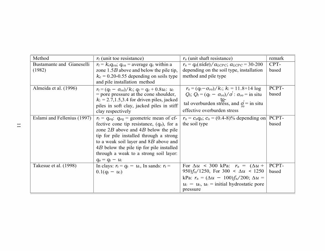
t 4 2

s

where kb = bearing capacity factor which depends on the soil type and is given in Table 2.4

and qca = average cone tip resistance computed as shown in Eq. 2.13.

qca = qca(A) + qca(B) 2

(2.13)

where qca(A), qca(B) = average cone tip resistances 3B above and below the pile tip respec-

tively [F/L2].

Table 2.4: kb values as a function of soil type

Soil type kb

Gravel 0.35 Sand 0.40 Silt 0.45 Clay 0.50

The unit shaft resistance, rs, is calculated from cone tip resistance as follows:

r = αs q Fs

≤ 120 kPa (2.14)

where Fs = an empirical factor that depends on the soil type and is given in Table 2.5, and

αs = a factor that depends on pile type. For precast concrete driven piles, αs = 1.25.

Table 2.5: Fs as a function of soil type

Soil type Fs Clay and calcareous clay 50 Silt, sandy clay, and clayey sand 60 Loose sand 100 Medium dense sand 150 Dense sand and gravel 200

2.3.6 Tumay and Fakhroo (1982)

Per (Tumay and Fakhroo, 1982) method, the unit toe resistance, rt, is computed in a similar

fashion with the Schmertmann (1978) method as follows:

r = qc1 + qc2 +

qa ≤ 15 MPa (2.15)

cs

17

L

where qc1 = average cone tip resistance below 4B below the pile tip [F/L2], qc2 = average

minimum cone tip resistance 4B below the pile tip [F/L2], and qa = average minimum cone

tip resistance 8D above the pile tip [F/L2], where B is the pile diameter [L].

The unit shaft resistance, rs, is proposed as shown below:

rs = mfca ≤ 72 kPa (2.16)

where fca = average load friction [F/L2] given in Eq. 2.17, and m = friction coefficient given

in Eq. 2.18. N

fca = i=1

LN

fi∆zi ∆zi

(2.17)

i=1

where fi = local sleeve friction at the ith soil layer [F/L2], ∆zi = depth of the ith soil layer,

and N = total number of soil layers.

m = 0.50 + 9.5 exp(−0.09fca) (2.18)

2.3.7 Prince and Wardle (1982)

According to this method, the unit toe resistance, rt, of piles was estimated from the cone

tip resistance, qc, using the following equation:

rt = kbqc ≤ 15 MPa (2.19)

where kb = an empirical factor that depends on the pile type. For driven piles, kb = 0.35

and for jacked piles, kb = 0.3.

The unit shaft resistance, rs, is computed from the local sleeve friction, fs, obtained from

a CPT test using the following relationship:

rs = ksfs ≤ 120 kPa (2.20)

where ks = an empirical factor that depends on the pile type. For driven piles, ks =0.53, for

18

jacked piles, ks = 0.62, and for bored piles ks = 0.49. 2.3.8 Bustamante and Gianeselli (1982)

This method was proposed by Bustamante and Gianeselli (1982) based on analyses of 197

pile loading tests with various bearing strata conditions. It is also known as the LCPC

(Laboratoire Central des Ponts et Chausees) method. The unit toe resistance, rt, per this

method is as follows:

rt = kcqca (2.21) where kc = bearing capacity factor given in Table 2.6, and qca = average cone tip resistance

[F/L2] determined based on the procedure outline in Figure 2.5.

Figure 2.5: Procedure for calculation of qca, after Bustamante and Gianeselli (1982)

The unit shaft resistance, rs, is estimated from the following equation:

r = qc(side) s α (2.22)

LCPC

19

Table 2.6: kc as a function of soil and pile type

Nature of soil kc

qc [MPa] Group I 1 Group II 2

Soft clay and mud 1 0.40 0.50 Moderately compacted clay 1 to 5 0.35 0.45 Silt and loose sand 5 0.40 0.50 Compacted to stiff clay and compacted silt 5 0.45 0.55 Soft chalk 5 0.20 0.30 Moderately compacted sand and gravel 5 to 12 0.40 0.50 Weathered to fragmented chalk 5 0.20 0.40 Compacted to very compact sand and gravel 12 0.30 0.40 1 plain bored piles; mud bored piles; micro piles (grouted under low pressure); cased bored

piles; hollow auger bored piles; piers; barrettes. 2 cast screwed piles; driven precast piles; prestressed tubular piles; driven cast piles; jacked

metal piles; micro piles (small diameter piles grouted under high pressure with diameter < 250 mm); driven grouted piles (low pressure grouting); driven metal piles; driven rammed piles; jacket concrete piles; high pressure grouted piles of large diameter.

where qc(side) = cone tip resistance for side layers [F/L2], and αLCP C = friction coefficient

given in Table 2.7. 2.3.9 Almeida et al. (1996)

According to this method, the unit toe resistance, rt, is obtained from:

r = qt − σv0 t k

(2.23)

2

where qt = cone tip resistance corrected for pore pressure effect [F/L2], σv0 = in situ over-

burden stress [F/L2], and k2 = a factor that depends on the pile and soil types; k2 = 2.7 for

driven piles, k2 = 1.5 for jacked piles in soft clay, and k2 = 3.4 jacked piles in stiff clay.

The unit shaft resistance, rs, is given by:

r = qt − σv0 s k

(2.24)

1

Table 2.7: αLCP C as a function of soil and pile type

Nature of soil qc

[MPa]

Category

Coefficients, αLCP C Maximum limit of rs I II I II III

Compact to stiff clay and compact silt > 5

≥ 0.2

1 plain bored piles; mud bored piles; hollow auger bored piles; micropiles (grouted under low pressure); cast screwed piles; piers; barrettes.

2 cased bored piles; driven cast piles. 3 driven precast piles; prestressed tubular piles; jacket concrete piles. 4 driven metal piles; jacked metal piles. 5 driven grouted piles; driven rammed piles. 6 high pressure grouted piles of large diameter ¿250 mm; micropiles (grouted under high pressure). * Note: maximum limit unit skin friction f: bracket values apply to careful execution and minimum disturbance of soil due to

construction

20

A 1 B 2

A 3 B 4

A B A B A 5 B 5

Soft clay and mud 5 30 90 90 30 0.015 0.015 0.015 0.015 0.035

Moderately compact clay 1 to 5 40 80 40 80 0.035 (0.08) *

0.035 (0.08)

0.035 (0.08)

0.035 0.08 ≤ 0.12

Silt and loose sand ≤ 5 60 60

150 120

60 60

120 120

0.035 0.035

0.035 0.035

0.035 0.035

0.035 0.035

0.08 0.08

-

(0.08) (0.08) (0.08) Soft chalk 5 100 120 100 12 0.035 0.035 0.035 0.035 0.08 -

Moderately compact sand and gravel 5 to 12 100 200 100 200 0.08 (0.12)

0.035 (0.08)

0.08 (0.12)

0.08 0.12 ≥ 0.2

Weathered to fragmented chalk > 5 60 80 60 80 0.12 (0.15)

0.08 (0.12)

0.12 (0.15)

0.12 0.15 ≥ 0.2

Compact to very compact sand and gravel > 12 150 300 150 200 0.12 (0.15)

0.08 (0.12)

0.12 (0.15)

0.12 0.15 ≥ 0.2

21

!

v0

t

where k1 is presented in Eq. 2.25.

k1 = 11.8 + 14 log Qt (2.25a)

Q = qt − σv0

v0

(2.25b)

where Qt = normalized cone tip resistance, σ! = in situ effective overburden stress [F/L2].

2.3.10 Eslami and Fellenius (1997) This method was proposed by (Eslami and Fellenius, 1997) based on 102 cases around the

world. The unit toe resistance, rt, is given as follows:

rt = qeq (2.26)

where qeq = the geometric mean of the effective cone resistance [F/L2], qe, for a zone 2B

above and 4B below the pile tip for a pile installed through a strong to a weak soil layer and

8B above and 4B below the pile tip for a pile installed through a weak to a strong soil layer

[F/L2]. qe is given by:

qe = qt − u2 (2.27)

where qt = corrected cone tip resistance for pore pressure effect [F/L2], and u2 = pore

pressure at the cone shoulder [F/L2].

Per (Eslami and Fellenius, 1997), the unit shaft resistance, rs, is given by:

rs = csqe (2.28)

where cs = an empirical coefficient, which is a function of soil type and is given in Table 2.8.

σ

22

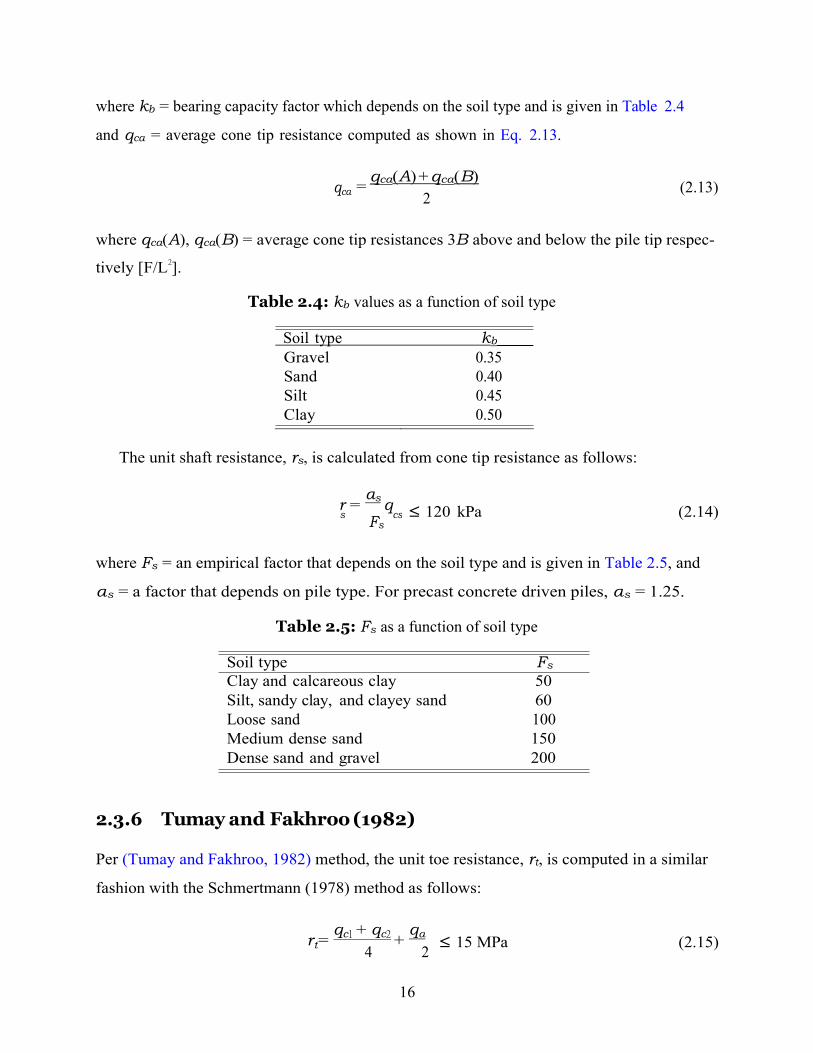
Table 2.8: cs as a function of soil types

Soil type cs(%) Soft sensitive soils 8.0 Clay 5.0 Stiff clay and mixture of clay and silt 2.5 Mixture of sand and silt 1.0 Sand 0.4

2.3.11 Takesue et al. (1998) In this method, the unit toe resistance, rt, in clay soils is similar to the Eslami and Fellenius

(1997) method. However, the unit toe resistance, rt, in sand soils is given by:

rt = 0.1qt (2.29)

where qt = corrected cone tip resistance for pore pressure effect [F/L2].

The unit shaft resistance, rs, is given as function of the measure pore pressure and local

sleeve friction during PCPT and is given according to the following equations:

rs = ∆u + 950

1250 fs (2.30a)

r = ∆u − 100 f s 200 s (2.30b)

where ∆u = u2 − u0, u0 = hydrostatic pore pressure [kPa], and fs = local sleeve friction

[kPa]. Eq. 2.30a is for ∆u < 300 kPa, and Eq. 2.30b is applied for 300 kPa < ∆u < 1250

kPa.

2.4 High Strain Dynamic Pile Testing (HSDPT) The high strain dynamic pile testing (HSDPT, ASTM-D4945 2008) has become a popular

tool to assess the installation process and bearing capacity of piles (Likins and Rausche,

2008). The key concept behind this test is that measurements retrieved during pile instal-

lation could be used to analyze the bearing capacity of piles since the driving process will

23

induce complete failure of the soils. Several studies have demonstrated the capability of the

HSDPT method to predict ultimate bearing capacity of pile accurately by comparing it with

the static pile loading test results (e.g. Likins and Rausche, 2004). The HSDPT may offer

reliable bearing capacity with relative advantages of overall cost minimization, less required

space, and less testing time as compared to static pile loading test. However, the HSDPT

needs thorough understanding of wave propagation mechanisms for accurate interpretation

of the test results.

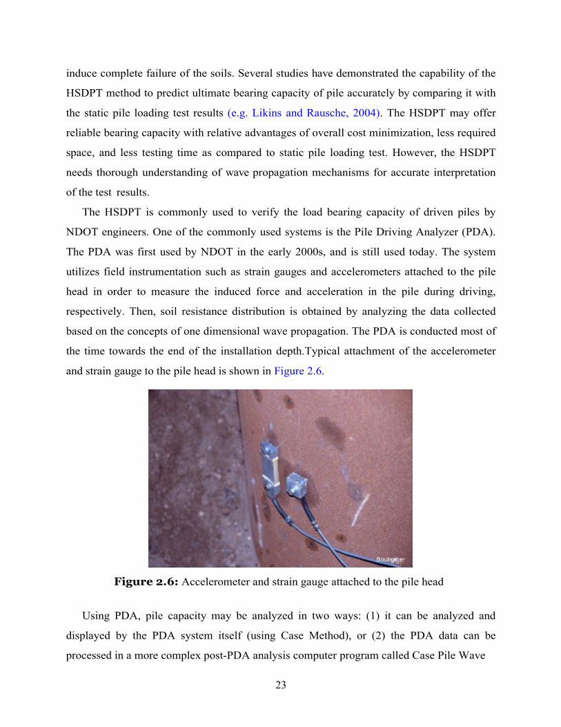
The HSDPT is commonly used to verify the load bearing capacity of driven piles by

NDOT engineers. One of the commonly used systems is the Pile Driving Analyzer (PDA).

The PDA was first used by NDOT in the early 2000s, and is still used today. The system

utilizes field instrumentation such as strain gauges and accelerometers attached to the pile

head in order to measure the induced force and acceleration in the pile during driving,

respectively. Then, soil resistance distribution is obtained by analyzing the data collected

based on the concepts of one dimensional wave propagation. The PDA is conducted most of

the time towards the end of the installation depth.Typical attachment of the accelerometer

and strain gauge to the pile head is shown in Figure 2.6.

Figure 2.6: Accelerometer and strain gauge attached to the pile head

Using PDA, pile capacity may be analyzed in two ways: (1) it can be analyzed and

displayed by the PDA system itself (using Case Method), or (2) the PDA data can be

processed in a more complex post-PDA analysis computer program called Case Pile Wave

24

2 c

Analysis Program (CAPWAP) for more accurate and reliable prediction. Both cases are

discussed in the next subsections.

2.4.1 Pile Capacity by PDA: Case Method

The total soil resistance is evaluated based on the measured force and velocity signals as well

as using information such as the pile geometry, pile material density and elastic modulus.

Typical force and velocity signals during the dynamic test is shown in Figure 2.7.

Figure 2.7: Typical force and velocity signals during dynamic test (source: Alvarez et al. 2006)

In the PDA, the Case Method (Rausche et al., 1985) is employed to compute the total

soil resistance from the measured velocity and force traces as shown in Eq. 2.31.

R(t∗) = 1

F

(t∗) + F

(t∗ +

2L

+ Z

v

(t∗) − v (

t∗ + 2L

(2.31) where R = total soil resistance [F], Fm = measured force [F], vm = measured velocity [L/T],

Z = impedance [M/T] , L = pile length [L], c = stress wave propagation speed (wave speed)

m m c 2 m m

25

I

[L/T], and t∗ = sampling time [T]. c and Z are given by the following equations:

c = E ρ

EA Z =

c

(2.32a) (2.32b)

where ρ = density of the pile material [M/L3] and A = pile cross-sectional area [L2]. Soil

resistance calculation using Eq. 2.31 consists of calculation of average internal forces at time

interval 2L/c apart and average acceleration for the same time interval. It could also viewed

be as an equation of motion with an average acceleration resulting from a resultant force

between the total soil resistance (external) and average internal forces within the pile. The

sampling time, t∗, is usually taken as the time at which the first major velocity peak occurs to ensure enough pile set and mobilization of the soil resistance. Moreover, due to rapid

penetration of the pile during impact driving, the total resistance depicted in Eq. 2.31 has a

dynamic part (velocity dependent) in addition to the static part (displacement dependent).

The total resistance (known quantity) is written as a summation of the static and dynamic

resistances as follows:

R = Rs + Rd (2.33) where Rs = static resistance [F], and Rd = dynamic resistance [F]. Since the total resistance

is known, the static resistance can be obtained if the dynamic resistance is determined. The

dynamic resistance is assumed to be proportional to the toe velocity as follows:

Rd = Jvb (2.34)

where vb = velocity of the pile toe [L/T], and J = viscous damping constant [FT/L]. In

this case, the damping is assumed to concentrate around the pile (Rausche et al., 1985).

By superimposing pile toe velocity in a free pile and pile velocity induced because of soil

resistance, and using Eq. 2.31 , the following equation, which represents the static resistance

26

c L

is obtained.

Rs(t∗

1 ) = (1

2 − jc) Fm

(t∗) + Zvm

(t∗)

1

+ (1 + 2

jc) Fm

(t∗ +

2L

− Zv (

t∗ + 2L

(2.35)

where Jc = (1/Z)J . Rausche et al. (1985) listed typical values of Jc by comparing a static

pile loading test and PDA results as shown in Table 2.9.

Table 2.9: Suggested values of Jc (after Rausche et al. 1985)

Soil type in bearing strata Suggested range, Jc Sand 0.05-0.20 Silty sand or sandy silt 0.15-0.30 Silt 0.20-0.45 Silty clay and clayey silt 0.40-0.70 Clay 0.60-1.10

The computed static resistance of soils based on the closed form solution shown in Eq.

2.35 assumes a rigid-plastic soil behavior and damping is concentrated around the pile tip.

The calculated soil resistance from Eq. 2.35 depends on the selection of Jc, and sampling

time, t∗. Moreover, to be consistent with the assumption of rigid-plastic soil behavior, this

method requires sufficient impact energy to be applied on the pile so that the induced pile set

is enough to mobilize all the available soil resistance. Thus, in a condition where the hammer

energy is small relative to the soil capacity, PDA may underpredict the pile capacity. Because

of all the aforementioned reasons, the Case Method is usually considered less reliable and

rather taken as a good first indicator of pile capacity (Likins and Rausche, 2008; Rausche

et al., 2017). 2.4.2 Pile Capacity by CAPWAP

A more realistic and reliable pile bearing capacity is computed by using CAPWAP (Case

Pile Wave Analysis Program) (Likins and Rausche, 2008). Unlike PDA, CAPWAP has

additional capabilities to model soil resistance distribution along the pile shaft and at the

toe, pile damping, splices, non-uniformity, and multiple shaft materials. It relies on signal

matching analysis (SMA) between the measured wave-up signal (obtained from the measured

m

27

L

velocity and force signals) with an artificially generated signal by varying the distribution of

soil resistance and other soil parameters along the pile shaft and at the pile toe.

The force, F (t), signal measured at the pile head (sensor location) can be split to down-

ward (wave-down) an upward (wave-up) moving components Rausche et al. (2010):

W (t) = 1

F (t) + Zv (t)]

(2.36a) d 2 m

W (t) = 1

F u 2 m

m

(t) − Zvm (t)]

(2.36b)

where Wd = wave-down [F ], and Wu = wave-up [F ]. The wave-down curve primarily repre-

sents the input from the hammer system, and the wave-up curve represent reflections from

soil resistance and pile non-uniformity. Assuming a uniform pile, the wave-up component

measured at the pile head is assumed to represent the soil resistance (Rausche et al., 1985):

n

Fm(t) − Zvm(t) = Ri(t) (2.37) i=1

where Ri = soil resistance at ith location out of n number of soil resistance concentrations

along the pile shaft [F]. This concept is illustrated in Figure 2.8, where the offset between

the Zv and F signals is the result of soil resistance. As previously noted, the soil resistance

is comprised of the static and dynamic components.

The wave-up SMA proceeds by first assuming the resistance distribution along with soil

parameters that define the static (quake) and dynamic (damping) resistances, and then

by taking the Zvm signal as a boundary condition, a complementary artificial force signal

is sought until a quality match is obtained with the measured complementary force, Fm,

signal. This SMA process may be performed interactively or automatically but, in general,

this process could be time consuming as the analysis evolves several unknown parameters

(including soil resistance, quake and damping) that need to be varied for the best match

(GRL engineers, 2018).

A numerical modeling technique that is either based on the lumped mass finite differ-

ence approach (Smith, 1962) or the method of characteristics (de Jong, 1956) is commonly

adopted to simulate the soil-structure interaction and perform the SMA. The CAPWAP

28

Figure 2.8: A miss-match between F and vmZ signals due to soil resistance (Source: Massarsch 2005)

signal mathcing analysis is typically based on the method of characteristics, where the pile

is divided into segments of 1 m length with elastic properties and optional pile damping

(GRL engineers, 2018). The static and dynamic behavior of the soil is modeled based on

the greatly expanded rheological model of Smith (1962), which incorporates elastoplastic

soil behavior (represented by spring and slider for the static component), and viscous and

radiation damping (represented by dashpot for the dynamic component). These soil resis-

tances are lumped at a certain interval along the pile shaft. A simplified traditional Smith

(1962) soil model is shown in Figure 2.9, which constitutes the spring and slider (static) and

dashpot (dynamic) systems.

The total soil resistance, which is lumped at a certain pile node, may be expressed as a

summation of the static and dynamic resistances, similar to the definition presented in Eq.

2.33 as follows:

R(t) = fglRs(t) + Rd(t) (2.38)

where fgl = gain/loss factor. The gain/loss factor is associated with soil set-up and

relaxation after pile driving. This factor is determined by performing a restrike test and by

comparing the static resistances during driving and after the restrike test (Rausche et al.,

29

Figure 2.9: Traditional soil resistance model (after Smith 1962)

2010). Generally, fgl is less than unity for the toe resistance while it is greater than unity

for the shaft resistance (Rausche et al., 2010).

The static resistance, Rs, versus pile displacement, u, relationship is modeled by a piece-

wise linear line, which is defined by soil parameters like gap and quake. The gap defines the

displacement upto which no static resistance develops, and quake defines the displacement

in excess of a gap in which the elastic response occurs or the relationship between Rs and

u is linear. Any pile displacement in excess of the gap plus quake is regarded as permanent

displacement and will mobilize the ultimate soil resistance. Separate values of quake are

assigned for the toe and shaft resistances, whereas gap is only assigned to the toe resistance

and taken as zero for the shaft resistance.

The dynamic resistance, Rd, is defined based on the basic (Smith, 1962) approach as

follows:

Rd(t) = jsRs(t)vp(t) (2.39)

where js = smith damping factor [T/L], and vp(t) = pile velocity [L/T]. Separate values of

smith damping, js, are assigned to the toe and shaft resistances. Then, the total resistance,

Rt could be rewritten as follows (assuming fgl = 1):

R(t) = Rs(t) (1 + jsvp(t)

] (2.40)

30

Therefore, in CAPWAP SMA, the following main variables are used: (1) assumed static

resistance distribution (toe and shaft resistances), (2) toe and shaft quake, and (3) toe and

shaft smith damping factors. Typical recommendations for the limits of CAPWAP soil

resistance parameters are provided in Table 2.10.

Table 2.10: Recommended values for limits of soil resistance parameters for CAPWAP SMA(after Rausche et al. 2010)

Parameter Shaft,min Shaft,max Toe,min Toe,max quake 1 mm 7.5 mm 1 mm umax − gap

js 0.04 s/m 1.4 s/m 0.04 s/m 1.4 s/m Match Quality in CAPWAP

The quality of signal matching between the measured and computed wave-up curves is a

very important aspect of CAPWAP that determines the accuracy of estimated pile bearing

capacity. In this regard, the strength of matching between the two curves is indicated by the

quantity, MQ, which stands for Match Quality in the CAPWAP user interface window. This

value is obtained by summing the absolute values of the difference between the measured

and computed wave-up curves. Since this difference has a unit of force, the result is further

divided by the maximum measured force to normalize it and make MQ a dimensionless

number (Rausche et al., 2010). There is no definite upper or lower bounds of MQ for an

acceptable CAPWAP result. In general, by generating the lowest possible MQ value, a

good correlation between dynamic and static test results could be achieved (e.g. Likins and

Rausche, 2004). Typical range of MQ is from 2 to 4, with values less than 0.5 being nearly

impossible and values greater than 6 producing unreliable capacity prediction (Rausche et al.,

2010).

Uniqueness of CAPWAP

Due to the large number of variables that need to be specified during the stress wave match-

ing process, the uniqueness of the solution obtained from CAPWAP has been regraded as

doubtful (e.g. Danziger et al., 1996; Buckley et al., 2017). Several studies outlined that

the particular soil resistance distribution obtained from CAPWAP is highly subjective and

31

can vary from one user to another. The question of uniqueness mainly emanates from the

discrepancy between the number of unknown variables and the number of available equa-

tions in the problem. The total number of primary unknowns that could significantly affect

the magnitude of mobilized soil resistance are 3N + 3, where N is the number of nodes on

the shaft. Shaft resistance, shaft quake, and shaft damping are unknowns per each node

on the shaft. The remaining three unknowns came from toe resistance, toe quake, and toe

damping. Although there are other unknowns in the problem, their affect on the predicted

soil resistance is negligible and they are only used for cosmetic improvement of the signal

matching (Buckley et al., 2017). In contrast, the available equations are equal to the number

of shaft and toe resistances (i.e. N + 1), as noted in Eq. 2.37. Since the number of unknowns

surpass the number of equations, it implies that parameter values in the problem have to be

iteratively changed until a good match is obtained. Different users may end up with different

sets of best fit soil parameter values leading to non-unique soil resistance distributions.

To investigate the uniqueness of CAPWAP results, Buckley et al. (2017) did signal match-

ing analysis using three independent users/operators on the same PDA result. Based on the

study conducted by Buckley et al. (2017), it was found that the CAPWAP soil resistance

distribution varied from user to user although the match quality fell within 1.7 to 1.9 for

all users. Particularly, a significant difference in the split between shaft and toe resistances

were obtained. However, the total resistance was found to vary within a ±10% from the mean among different users.

2.4.3 Pile Setup and Relaxation

Based on extensive field investigations, it is recognized that pile capacity may increase with

time. This time dependent increase in pile capacity is known as pile setup or freeze. This

phenomenon is almost common in all types of driven piles (although more significant in

displacement piles) embedded in saturated clay, loose to medium silt, sandy silt, silty sand,

and fine sand (Komurka et al., 2003). The opposite of pile setup may occur in piles embedded

in dense silts, weathered shale (Rausche et al., 2010), and heavily overconsolidated clays

(Jardine and Bond, 1989), where the pile capacity decreases with time. This phenomenon is

termed as pile relaxation or negative pile setup.

32

The complete mechanism of pile setup is not fully understood. However, the majority of

the pile setup is attributed to the dissipation of pore pressure at the end of driving (EOD)

and subsequent increase in effective stress, which in turn causes an increase in soil resistance.

Based on this mechanism, a long-term setup is expected in cohesive (e.g. clay) and mixed

soils (e.g. clayey fine sand, clayey silt) and, whereas a short-term pile setup is expected

in sand soils and gravels. It is reported, however, that a long-term pile setup may occur

in fine grained sand soils and silts owing partly due to the breakdown of a driving-induced

arching effect on the pile shaft and partly due to aging (effect of creep) (Axelsson, 2002).

Moreover, several research findings have indicated that pile setup primarily influences the

shaft resistance due to the substantial lateral displacement and eventual stiffening of the

adjacent soils during pile installation (Fellenius et al., 2000).

On the other hand, negative pile setup (pile relaxation) could be possible in dilatant

soils (e.g. dense to very dense silts and fine sands and heavily overconsolidated soils) where

effective stress temporarily increases during pile installation due to the development of a

negative excess pore pressure and thereafter, decreases as the negative excess pore pressure

is dissipated (Jardine and Bond, 1989; Komurka et al., 2003). In addition to this, weathered

shale and weak laminated rocks (Hannigan et al., 1997; Rausche et al., 2010) may experience

pile relaxation. As opposed to pile setup, pile relaxation is thought to have more influence

on toe resistance than shaft resistance (Komurka et al., 2003; Rausche et al., 2010).

Incorporating the effect of pile setup/relaxation in the design of piles can provide an

economical design by either reducing the length or the number of piles required in the

design. However, the availability of reliable and feasible methods to obtain the magnitude

of pile setup/relaxation is seldom (Ng et al., 2012). In current practice, measurement of pile

setup/relaxation may be possible based on static or dynamic tests (restrike test) conducted at

different times after EOD. However, when using these tests, the cost saving by accounting pile

setup/relaxation into the pile design often needs to be justified with the cost of performing

the tests for an extended period. Apart from direct measurement using instrumented field

tests, empirical correlations has been proposed in the literature (e.g. Skov and Denver, 1988)

to predict pile setup in particular. These equations are site specific and may need calibration

using restrike tests to determine some of the constants in the equations; plus, they are not

33

extensively validated for practical application (Ng et al., 2012). 2.5 Conclusions

The general form of the CPT/PCPT-based methods reviewed is similar. However, each

method proposed different values for the empirical coefficients depending on the type of pile

and soil conditions they were derived in. Since the methods are site specific, their application

to a different site condition should be preceded by proper evaluations and calibrations of the

methods using reliable pile capacities determined from either static or dynamic loading tests

(HSDPT).

Several studies have shown the validity of the HSDPT to be a reliable approach to predict

pile capacity through comparative studies with static load test results. Besides its reliability,

the HSDPT is advantageous because it provides cost savings, and requires less space as well

as less testing time. One of the widely-used HSDPT system is the PDA. The PDA may

provide pile capacity in two ways: one is within the PDA system itself and the other is using

a post analysis tool called CAPWAP. Due to a more detailed modeling of the soil-structure

interaction in CAPWAP, it is regarded as a more reliable and accurate tool to obtain pile

capacity as compared to the results obtained from the built-in logic within the PDA. Due

to the involvement of several unknown parameters in CAPWAP analysis, the uniqueness of

the soil resistance distribution obtained by this method has been questionable. Furthermore,

the CAPWAP provides pile capacity available at the time of testing. But, multiple studies

have shown that pile capacity may vary with time due the effect of pile setup/relaxation.

The pile setup/relaxation phenomenon is primarily a function of soil type and pile geometry.

Moreover, pile setup is usually more pronounced on the shaft resistance, and pile relaxation

is prominent on the toe resistance. To account for these effects, usually a restrike test is

conducted after a certain period of elapsed time from EOD.

34

Chapter 3 METHODOLOGY 3.1 Introduction

The primary objective of this research was to evaluate different CPT/PCPT-based pile

prediction models and propose a modified method that is applicable for Nebraska soil con-

ditions. To achieve this goal, data were collected from NDOT for bridge site locations that

had the following records: (1) driven pile records, (2) dynamic load test data, (3) boring

information, and (4) PCPT records. These data were used to evaluate the in-place capacity

of the piles (considered as measured pile capacity) installed at the bridge sites. On the other

hand, the CPT/PCPT-based methods discussed in the previous chapter were used to predict

pile capacities. The measured and predicted pile capacities were compared and evaluated

to distinguish the best performing method(s) using the rank index (RI). Furthermore, the

same PCPT data excluding the pore pressure measurements was used in the CPT-based

methods.

3.2 Test Sites The test sites were selected in order to obtain representative soil conditions for the majority

of the existing bridge site locations as well as potential future bridge foundation work. Two

factors primary influenced the selection of the test sites. First, not all soil conditions in

Nebraska are favorable for PCPT investigations; second, the availability of the load test

data (PDA).

Sites with significant layers of dense sand and gravel that offer high bearing resistance

at relatively shallower depths are difficult to be penetrated by the pushed CPT equipment.

This is certainly one of the limitations of the CPT (Robertson and Cabal, 2010). Thus,

most of the sites selected are composed of softer, and fine-grained materials. In fact, as pile

35

foundations are normally required in such soil conditions, it is logical to restrict the site

selection tending towards these types of materials. Although sites with relatively thin layers

of granular (coarse grained) soil conditions were included in the bearing capacity evaluations,

those sites with thick layers (more than 15 m) of dense sand and gravel (highly angular),

which are typically abundant in the western Nebraska, were disregarded.

In NDOT practice, the PDA is mainly used as a verification to ensure whether the design

capacity is met and to monitor pile drivability to help construction engineers decide project-

specific pile driving adjustments. Considering this, PDA is usually conducted on piles that

support structures of high importance and with high load capacity. In other scenarios, the

PDA is implemented on structures selected based on cost/benefit analysis, and the variability

of the soil condition. Thus, bridge structures that had complete PCPT logs as well as PDA

results were compiled and used for further analyses. Figure 3.1 shows the location of sites

selected in this study.

Figure 3.1: Locations of sites selected in this study

The site selection process resulted in a total of 14 projects which are comprised of 16

bridges structures. Each bridge structure was further comprised of substructures (i.e. Abut-

ments and Piers). For each substructure, their corresponding PCPT and PDA results were

organized. In some cases, common PCPT data was shared for two substructures which are

adjacent to each other. In other cases where quality PDA results exist but PCPT data is

absent, NDOT staff conducted new PCPT to have a complete data set of PDAs as well as

36

PCPT. 3.3 Piles

The pile data base consisted of steel H-piles, closed end pipe piles and precast prestressed

concrete (PPC) piles. H-piles most commonly used by NDOT are HP10x42, HP12x53, and

HP14x89 sizes. Steel pipe piles are almost all 12.75” O. D. with 3/8 in. wall thickness and

welded plate bottoms. A prestressed concrete pile used by the state can be square, circular,

or hexagonal with 28-day strength ranging from 4000-5000 psi. In this study H-piles, pipe

piles, and square precast prestressed concrete piles (PPC) were evaluated. 45 H-piles, 41

pipe piles, and 6 PPC cases were analyzed.

3.4 PCPT Data

PCPT data was acquired from the logging software in [*.csv] format. The log information

consisted of depth, tip resistance (qc), local sleeve friction (fs), and pore pressure at the

cone shoulder (u2) data that was measured as the cone penetrated through the ground. The

PCPT data also provided soil classification based on the Robertson et al. (1986) soil behavior

type (SBT ) chart. 3.5 Soil classification

Soil classification was necessary in order to determine the appropriate values of empirical

coefficients, which are dependent on the type of soils in the CPT/PCPT-based methods. To

alleviate the need for soil sampling and subsequent laboratory testing to classify the soils,

the PCPT data itself was used to identify the type of soils based on previously established

CPT-based soil classification methods. Several CPT-based soil classification charts had been

proposed in the past (Douglas and Olson, 1981; Robertson et al., 1986; Robertson, 1990).

Among these methods, the Robertson et al. (1986) soil classification results at 2 cm interval

were directly available along with qc, fs, and u2 data.

37

The Douglas and Olson (1981) soil classification method was regarded as the most com-

prehensive. However, it is too complicated for practical application (Bloomquist et al., 2007).

After that, Robertson et al. (1986) came up with a soil behavior type (SBT ) classification

chart that was easier to apply. Despite its simplicity, it had one major shortcoming in that

the effect of the depth of penetration on the cone tip resistance values was not incorporated

in the soil classification scheme (Bloomquist et al., 2007). For this reason, it is believed that

some error could be introduced eventually when this chart is used to classify soils below

30 m (100 ft). However, since most on-shore pile foundations are within this range, this

shortcoming may not pose a significant problem. Later on, by properly accounting for the

effect of depth, Robertson (1990) proposed an updated normalized soil behavior type chart

(SBTn) where, the cone tip resistance was normalized with the overburden stress to address

the influence of depth.

To this end, the CPT-based soil classification chart proposed by Robertson et al. (1986)

was used in this study considering that: (1) the pile foundations in NDOT’s bridge con-

struction practice may not extend beyond 30 m, (2) the Robertson et al. (1986) soil classi-

fication output was readily available within the PCPT data acquired from NDOT, and (3)

the method was easier to apply and implement in program coding. The Robertson et al.

(1986)classification chart is shown in Figure 3.2 below.

Figure 3.2: Soil Behavior Type (SBT ) chart, after Robertson et al. (1986)

38

3.6 Dynamic Load Test Data The CAPWAP processed PDA signals are used to yield the reference pile capacities. For the

purpose of this study, PDA results over the entire installation length of the pile were used

because this could maximize the utilization of a single PCPT data for several CPT-PDA

correlations at different depths. The match quality, MQ, was kept as low as possible to

ensure accurate pile capacity predictions.

Owing to the uncertainty about the uniqueness of CAPWAP soil resistance distribution,

which may result in an unreliable split between shaft and toe resistances, this study used

the gross soil resistance as a reference pile capacity. Thus, the gross pile capacity predicted

via CAPWAP is evaluated against the summation of toe and shaft resistances predicted via

CPT/PCPT-based methods.

Moreover, the effect of pile setup/relaxation effects needs to be addressed. From the

general soil condition of Nebraska, it is possible that driven piles, especially in eastern Ne-

braska, may pass through cohesive soils, fine grained granular soils, and overconsolidated

glacial tills. Therefore, it is expected that both short-term as well as long-term pile setup

may be possible. On top of this, the presence of overconsolidated soils and shale also present

the possibility of pile relaxation. Thus, appropriate evaluation needs to account for both

pile setup and relaxation in the pile capacity evaluation. The current dynamic test results

(PDA) available in this study corresponds to EOD condition and unfortunately, due to the

lack of restrike pile capacity data set along with the EOD data set, the quantification of

pile setup/relaxation for a reasonably accurate pile capacity evaluation was not performed

in this study. The use of empirical equations was not favored as they are mainly proposed to

predict pile capacity increment (setup), and they may result in unnecessarily overestimating

the pile capacity because the effect of relaxation may prevail as well. Based on engineering

judgment, the effect of pile setup/relaxation was disregarded in this study. The increase in

shaft resistance (setup) may be counterbalanced by the decrease in the toe resistance (re-

laxation) and disregarding the effect of pile setup/relaxation may be justified in this regard.

However, the authors suggest collecting and analyzing future EOD and restrike dynamic test

results for the assimilation of Nebraska-specific pile setup/relaxation factors in the future.

39

3.7 In Place Pile Capacity from Pile Driving Records Driving records were also used to predict the pile capacity using the current NDOT LRFD

(load resistance factor design) approach based on the EN (Engineering News) formula as

shown in Eq. 3.1. This equation represents an official and well-verified bearing capacity

estimation method for driving piles in Nebraska.

4E φQu = s + 0.5 (3.1)

where Qu = ultimate (nominal) pile capacity [F], E = hammer energy defined by E = WH,

where W = ram weight of the hammer [kips], H = fall height of the ram [ft.], and s = pile

set [in/blow], and φ = resistance factor = 0.7. The proposed CPT/PCPT-based method

was compared with pile capacities estimated based on Eq. 3.1.

3.8 Evaluation Methodology Performance evaluation of the CPT/PCPT-based methods was performed using statistical

analyses as well as non-statistical analyses. Several researchers adopted the same technique

to assess the prediction capability of CPT/PCPT based methods in the past (e.g. Briaud

and Tucker, 1988; Long and Wysockey, 1999; Abu-Farsakh and Titi, 2004; Cai et al., 2009;

Nguyen et al., 2016). Relying entirely on statistical analyses may lead to misleading con-

clusions regarding the performance of the methods (Briaud and Tucker, 1988). Thus, it is

usually recommended to inspect the predicted versus measured pile capacity plots before

passing judgment on the prediction capability of a method.

Henceforth in this report, the measured pile capacity, which was obtained from CAPWAP,

is designed by Qm and sometimes also referred to as QP DA in this report; the predicted pile

capacity, which was obtained based on the CPT/PCPT methods, is designated by Qp and

sometimes will be designated as QCP T . The ratio Qp/Qm has an optimum value of 1 for

a perfect prediction ,and away from this optimum scenario, it may be less than unity or

40

L

greater than unity for underprediction and overprediciton, respectively. The least possible

Qp/Qm is 0 and the highest is positive infinity (+∞).

Before carrying out the evaluation of the CPT/PCPT-based methods, piles were catego-

rized as displacement and non-displacement piles as the mechanism of load support is differ-

ent in these types of piles. In this regard, H-piles were categorized under non-displacement

piles, where toe resistance is assumed to be the predominant source of total pile capacity. On

the other hand, pipe piles and PPC were categorized as displacement piles in which major

load resistance comes from shaft resistance.

Thereafter, different statistical and plot-based evaluation schemes were applied to the

ratio Qp/Qm in order to assess the relative accuracy and precision of the CPT/PCPT-based

methods. The accuracy and precision of prediction is mainly depicted by the central tendency

or the mean and the standard deviation of Qp/Qm, respectively(Briaud and Tucker, 1988).

The particular method is accurate if the mean is closer to 1 ,and precise when the standard

deviation is closer to zero. Based on previous works, statistical criteria incorporating the

above measures as well as other non-statistical measures that showed the quality of Qp vs

Qm plots were used in the evaluation process (Briaud and Tucker, 1988; Long and Wysockey,

1999; Abu-Farsakh and Titi, 2004; Eslami et al., 2011). The evaluation scheme adopted the

following four criteria: 1. The slope of√the best fit line between Qp and Qm and the square root of residual sum

of squares ( RSS) between perfect prediction (Qp,best) and Qp.

2. The coefficient of variation (COV ) of Qp/Qm.

3. The 50% (P50) and 90% (P90)cumulative probabilities.

4. The ±20% accuracy from histogram and lognormal distribution of Qp/Qm.

A rank (Ri) was used to indicate the performance of a given CPT/PCPT-based method

for the ith criterion. Finally, a rank index (RI) was used to determine the overall performance

by simply summing each Ri from each criterion, as shown in Eq. 3.2. The method with the

lowest RI was considered as the best performing method.

4

RI = Ri (3.2) i=1

41

L

Details of the each criterion is described in the following subsection. 3.8.1 Criterion 1

The first criterion is comprised of two sub-criterion. The first sub-criterion compares the

magnitude of the slope of the best-fit line passing through the origin for the Qp vs Qm plot. It

reveals the tendency of a given CPT/PCPT method to either overestimate or underestimate

the measured pile capacity, Qp. The best method is considered to be the one with a slope

closer to 1.

The second sub-criterion was the square root of the residual sum of squares (√

RSS)

between an ideal (perfect) prediction (Qp,ideal) and actual prediction (Qp). This sub-criterion

shows the accumulated deviation of a given CPT/PCPT method from the ideal scenario.

The higher the √

RSS is, the lower the performance of the method, and vice versa. The

two criteria are shown in Figure 3.3. For instance, the slope of the best-fit line in Figure 3.3

shows underprediction. Based on Figure 3.3, the square root of the residual sum of squares

was computed as:

RSS =

N

i=1

(Qp,i − Qm,i)2 (3.3)

where Qp,i = predicted pile capacity by the CPT/PCPT method [F], and Qm,i = measured

pile capacity using CAPWAP [F]. The rank for criterion 1 was obtained by summing the

sub-ranks obtained from corresponding sub-criteria.

3.8.2 Criterion 2

The second criterion was the coefficient of variation (COV ). COV is obtained by normal-

izing the standard deviation by the mean for the Qp/Qm data set as shown in Eq. 3.4.

This statistical measure shows the extent of data scattering relative to the mean and it is

considered to be indicative of the precision of the CPT/PCPT-based methods. Generally,

the lower the COV , the better the performance of the method.

σ COV =

µ

(3.4)

√

42

Figure 3.3: Slope of the best-fit line and residuals

where σ = standard deviation of Qp/Qm, and µ = mean of Qp/Qm.

3.8.3 Criterion 3

The third criterion was based on the 50% (P50) and 90% (P90) cumulative probabilities.

These statistical measures were computed by arranging the Qp/Qm ratio in ascending order

and then using the following equation (Long and Wysockey, 1999):

i P =

n + 1

(3.5)

where i = order number, and n = total number of Qp/Qm ratios.

This criteria was comprised of two sub-criteria. The first sub-criterion was the magnitude

of P50. P50 shows the particular Qp/Qm value halfway through the data and depicts the

tendency of the method to either underestimate or overestimate pile capacity. This measure

is more advantageous than simply computing the mean because the mean could be biased by

the largest and smallest Qp/Qm values. The closer P50 is to 1, the better the performance of

the method. The second sub-criterion was the difference between P90 and P50. The smaller

this difference is, the better the performance of the method because it shows reduced scatter

43

f (x) = √2πσ

exp x

− 2

of Qp/Qm values above the P50 value. The rank for criteria three was obtained by summing

the sub-ranks corresponding to each sub-criterion.

3.8.4 Criterion 4

The fourth criterion evaluated the ±20% accuracy level based on the histogram and log-

normal distribution. As the name implies, these measures depict what probability of the

predicted pile capacity will be within 0.8Qm ≤ Qp ≤ 1.2Qm range. Rather than using a

single mean value as a measure of accuracy, the ±20% accuracy level is advantageous given

that little room for variation of Qp/Qm is allowed.

Due to the possible variation of Qp/Qm from 0 to +∞ with an optimum value of 1, the

distribution of Qp/Qm is unsymmetrical about the mean (Briaud and Tucker, 1988) and thus

the log-normal distribution is recommended to mimic the probability distribution of Qp/Qm.

There were two sub-criteria in this category. In the first sub-criterion, the ±20% accuracy

level was obtained based on the histogram plot. In the second sub-criterion, it was obtained

based on log-normal distribution assumption. Although both sub-criteria reveal the same

measure, one is based on measured values, and the other is based on assumed probability

distribution using the mean and standard deviation of the measured values (forecast the gen-

eral trend). The histogram was drawn by considering the frequency Qp/Qm in a certain bin

size, while the log-normal distribution was obtained by using a probability density function,

f (x), shown in Eq. 3.6 following (Abu-Farsakh and Titi, 2004).

1 1 (

ln(x) − µln 2

where x = Qp/Qm , µln = mean of ln(Qp/Qm), and σln = standard deviation of ln(Qp/Qm).

The rank for criterion 4 was obtained by summing the sub-ranks corresponding to each sub-

criterion.

ln ln σ (3.6)

44

N

3.9 Calibration Methodology After carrying out the evaluation of all the CPT/PCPT-based methods, it was found that

some methods show better performance in terms of precision and weak performance in terms

of accuracy. As discussed in the previous chapter, the methods are empirical and site specific.

To improve the prediction accuracy of those methods, a calibration was performed. The

calibration process mainly followed a procedure of minimizing the squared residual between

the measured and predicted pile capacities aiming to enhance the accuracy of the methods.

Separate calibration factors were assigned to the predicted toe and shaft resistances from

the CPT/PCPT methods for displacement (HP piles) and non-displacement (PP and PPC

piles). The following basic logic was employed to calibrate the CPT/PCPT-based methods:

Minimize ⇒ RSS =

L

i=1

Qm,i − (

ηQt,i + θQs,i

2 (3.7)

where Qt = predicted toe capacity [F], Qs = predicted shaft capacity [F], and η, θ = calibra-

tion factors corresponding to toe and shaft resistance, respectively. η and θ are different for

H-piles, pipe piles, and PPC piles. The MS-Excel application was used to perform the above

calibration process. After the calibration of each method, re-evaluation was performed using

the criteria discussed in Section 3.8.

45

2 1

Chapter 4 RESULTS AND DISCUS-

SIONS 4.1 Introduction

The performance of the CPT/PCPT-based pile design methods was evaluated based on

the criteria discussed in the previous chapter, and results are presented in this chapter.

The CAPWAP database was subdivided to a category of H-piles, pipe piles, and PPC piles

and results of the evaluation are presented for each category separately. The chapter is

organized in a way that first, an evaluation on the original CPT/PCPT-based methods is

presented, and then an evaluation of the calibrated methods is presented. A comparison of

the improvements on the performance of the methods was performed and discussed. Finally,

the best performing methods were identified and compared with the NDOT LRFD- based

pile driving formula results. The risk of Qp being greater than Qm was also compared between

the best performing methods and the NDOT LRFD-based pile driving formula following a

simple probabilistic analysis (Briaud and Tucker, 1988).

4.2 Initial Evaluation 4.2.1 H-Piles

Criterion 1

The first sub-criterion in this category was the slope of the best-fit line between Qp and Qm.

Table 4.1 shows the summary of the sub-ranks for this sub-criterion, and Figure 4.1 shows

the best-fit line for Qp vs Qm plots of the first top four best performers. In Table 4.1, R1∗ and

R∗ denote the sub-ranks for the slope of the best-fit line and √

RSS criteria. R denotes the

46

p m

overall rank for criterion 1. The Bustamante and Gianeselli (1982) method underestimated

pile capacity and the other methods generally overestimated it.

The second sub-criterion, which was the square root of the residual sum of squares, showed

that Price and Wardle (1982); Bustamante and Gianeselli (1982); Aoki and de Alencar (1975)

performed well and obtained rank from 1st to 3rd, respectively.

Table 4.1: The slope of the best-fit line between Q and Q and √

RSS for H-piles

CPT/PCPT-based method Qp vs Qm

√RSS R∗ R∗ R∗ + R∗ R

slope 1 2 1 2 1

Aoki and de Alencar (1975) 1.019 2672.36 1 3 4 2 Clisby et al. (1978) 0.574 3375.01 8 5 13 6 Schmertmann (1978) 1.309 4038.94 5 6 11 5 De Ruiter and Beringen (1979) 1.574 5200.99 9 9 18 9 Philipponnat (1980) 1.392 4400.78 7 7 14 7 Tumay and Fakhroo (1982) 1.268 3254.91 4 4 8 4 Price and Wardle (1982) 1.050 2358.93 2 1 3 1 Bustamante and Gianeselli (1982) 0.882 2494.17 3 2 5 3 Almeida et al. (1996) 1.381 4442.87 6 8 14 7 Eslami and Fellenius (1997) 1.977 8535.83 10 10 20 10 Takesue et al. (1998) 2.728 20414.43 11 11 22 11

Criterion 2 Based on this criterion, the precision of the CPT/PCPT-based methods was evaluated. Table

4.2 summarizes the results for this criterion. The De Ruiter and Beringen (1979) method

showed the best precision. The Price and Wardle (1982) and Philipponnat (1980) followed

second and third, respectively. The De Ruiter and Beringen (1979) method was found to

perform relatively the worst in the previous criterion with a rank of 9. This clearly shows

that the accuracy of the De Ruiter and Beringen (1979) method is poor whereas its precision

is relatively excellent. As a justification for its poor accuracy, Table 4.6 shows the mean value

of Qp/Qm is substantially high, which means it overestimated pile capacity substantially.

Criterion 3 The 50% (P50) and 90% (P90) cumulative probabilities were compared and ranks were ob-

tained form this criterion. Table 4.3 summarizes the results of this criterion. The Aoki and

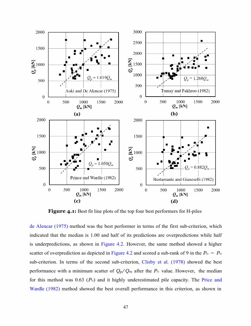
47

(a) (b)

(c) (d)

Figure 4.1: Best fit line plots of the top four best performers for H-piles de Alencar (1975) method was the best performer in terms of the first sub-criterion, which

indicated that the median is 1.00 and half of its predictions are overpredictions while half

is underpredictions, as shown in Figure 4.2. However, the same method showed a higher

scatter of overprediction as depicted in Figure 4.2 and scored a sub-rank of 9 in the P90 − P50

sub-criterion. In terms of the second sub-criterion, Clisby et al. (1978) showed the best

performance with a minimum scatter of Qp/Qm after the P50 value. However, the median

for this method was 0.63 (P50) and it highly underestimated pile capacity. The Price and

Wardle (1982) method showed the best overall performance in this criterion, as shown in

48

Table 4.2: COV in the ratio Qp/Qm for H-piles

CPT/PCPT-based method σ µ COV R2 Aoki and de Alencar (1975) 0.56 1.24 0.455 9 Clisby et al. (1978) 0.23 0.66 0.351 5 Schmertmann (1978) 0.70 1.55 0.450 8 De Ruiter and Beringen (1979) 0.61 1.86 0.326 1 Philipponnat (1980) 0.57 1.65 0.347 3 Tumay and Fakhroo (1982) 0.53 1.50 0.350 4 Price and Wardle (1982) 0.40 1.20 0.339 2 Bustamante and Gianeselli (1982) 0.52 1.09 0.473 10 Almeida et al. (1996) 0.58 1.65 0.353 6 Eslami and Fellenius (1997) 0.88 2.37 0.370 7 Takesue et al. (1998) 2.62 3.12 0.841 11

Table 4.3.

Table 4.3: 50% and 90% cumulative probabilities in the ratio Qp/Qm for H-piles

CPT/PCPT-based method P50 P90−P50 R1∗ R2

∗ R1∗ + R2

∗ R3

Criterion 4

The relative accuracy of the CPT/PCPT-based methods over a range of ±20% overpredic-

tion/underprediction was evaluated with this criterion. Table 4.4 and Figure 4.3 show the

results from this evaluation. The sub-criteria in this category were similar except one was

based on histogram and the other was based on log-normal distribution obtained from the

mean and standard deviation of ln(Qp/Qm). The Price and Wardle (1982) showed the best

performance with an accuracy of ~ 58%. Then, the method of Aoki and de Alencar (1975)

Aoki and de Alencar (1975) 1.00 1.08 1 9 10 5 Clisby et al. (1978) 0.63 0.37 6 1 7 2 Schmertmann (1978) 1.35 0.85 5 4 9 3 De Ruiter and Beringen (1979) 1.77 0.75 9 3 12 7 Philipponnat (1980) 1.55 0.96 8 6 14 8 Tumay and Fakhroo (1982) 1.32 0.85 4 5 9 3 Price and Wardle (1982) 1.18 0.54 3 2 5 1 Bustamante and Gianeselli (1982) 0.89 1.07 2 8 10 5 Almeida et al. (1996) 1.46 1.11 7 10 17 9 Eslami and Fellenius (1997) 2.23 1.06 11 7 18 10 Takesue et al. (1998) 2.23 4.26 10 11 21 11

49

(a) (b)

Figure 4.2: Cumulative probabilities of the ratio Qp/Qm values for H-piles

and Bustamante and Gianeselli (1982) showed the best second and third performances, re-

spectively.

Table 4.4: ±20% accuracy level based on histogram and log-normal distribution for H-piles

CPT/PCPT-based method Histogram Log- R∗ R∗ R∗ + R∗ R normal 1

2

1

2 4

Aoki and de Alencar (1975) 61.36 % 53.14 % 1 3 4 2 Clisby et al. (1978) 40.91 % 33.51 % 5 6 11 6 Schmertmann (1978) 45.45 % 36.65 % 4 5 9 4 De Ruiter and Beringen (1979) 13.64 % 15.60 % 10 10 20 10 Philipponnat (1980) 27.27 % 29.01 % 7 8 15 7 Tumay and Fakhroo (1982) 40.91 % 37.17 % 5 4 9 4 Price and Wardle (1982) 59.09 % 57.68 % 2 1 3 1 Bustamante and Gianeselli (1982) 54.55 % 55.93 % 3 2 5 3 Almeida et al. (1996) 22.73 % 30.10 % 8 7 15 7 Eslami and Fellenius (1997) 6.82 % 6.76 % 11 11 22 11 Takesue et al. (1998) 20.45 % 18.17 % 9 9 18 9

Rank Index, RI

The overall rank of all CPT/PCPT based methods was computed by comparing the RI,

which is simply the sum of all the ranks from each criterion (1 ~ 4). Table 4.5 shows the

summary of the RI and the overall ranks for H-piles. Based on this table, the Price and

50

(a) (b)

(c) (d)

Figure 4.3: Histogram and log-normal distribution plots of the top four best performers for H-piles

Wardle (1982) method stood first and thus considered the best performing method. The

Tumay and Fakhroo (1982) and Aoki and de Alencar (1975) methods were the second and

third best performers with a RI of 15 and 18, respectively. However, as per the RI value, it

is clear that these methods were significantly outperformed by the Price and Wardle (1982)

method.

51

Table 4.5: Rank index (RI) and overall ranks of each CPT/PCPT-based methods for H-piles

CPT/PCPT-based method Cr. 1 Cr. 2 Cr. 3 Cr. 4 RI Rank Aoki and de Alencar (1975) 2 9 5 2 18 3 Clisby et al. (1978) 6 5 2 6 19 4 Schmertmann (1978) 5 8 3 4 20 5 De Ruiter and Beringen (1979) 9 1 7 10 27 8 Philipponnat (1980) 7 3 8 7 25 7 Tumay and Fakhroo (1982) 4 4 3 4 15 2 Price and Wardle (1982) 1 2 1 1 5 1 Bustamante and Gianeselli (1982) 3 10 5 3 21 6 Almeida et al. (1996) 7 6 9 7 29 9 Eslami and Fellenius (1997) 10 7 10 11 38 10 Takesue et al. (1998) 11 11 11 9 42 11

4.2.2 Pipe and PPC Piles

Criterion 1

For pipe and PPC piles, the Price and Wardle (1982) and Bustamante and Gianeselli (1982)

were equally the best performance, as shown in Table 4.6 and Figure 4.4. Both methods

seem to very slightly overpredict pile capacity (by ~ 1%). Aoki and de Alencar (1975) was

the third best performing method in this criterion. In terms of the √

RSS sub-criterion, both

the Price and Wardle (1982) and the Bustamante and Gianeselli (1982) methods nearly had

the same square root of residual sum of squares and clearly outperformed the other methods.

Criterion 2 In this category, the Tumay and Fakhroo (1982) method performed excellent as shown in

Table 4.2. The Eslami and Fellenius (1997)and De Ruiter and Beringen (1979) methods

followed second and third, respectively. Similar to the previous case, the Tumay and Fakhroo

(1982) method had the best precision for pipe and PPC piles. However, its accuracy was

poor and therefore its performance in criterion 1 was ultimately poor. In support of this, the

mean value of this method showed that it overpredicted pile capacity on average by about

60%.

52

p m Table 4.6: The slope of the best-fit line between Q and Q and √

RSS for pipe and PPC piles

CPT/PCPT-based method Qp vs Qm √

RSS R∗ R∗ R∗ + R∗ R1 1 2 1 2

Aoki and de Alencar (1975) 1.034 3069.78 3 3 6 3 Clisby et al. (1978) 0.555 3635.93 8 5 13 6 Schmertmann (1978) 1.235 4078.80 5 6 11 5 De Ruiter and Beringen (1979) 1.477 4841.62 9 7 16 8 Philipponnat (1980) 1.385 4969.71 6 8 14 7 Tumay and Fakhroo (1982) 1.224 3469.95 4 4 8 4 Price and Wardle (1982) 1.010 2915.20 1 2 3 1 Bustamante and Gianeselli (1982) 1.011 2896.55 2 1 3 1 Almeida et al. (1996) 1.414 4980.01 7 9 16 8 Eslami and Fellenius (1997) 1.833 7911.30 11 11 22 11 Takesue et al. (1998) 1.503 6806.36 10 10 20 10

Table 4.7: COV in the ratio Qp/Qm for pipe and PPC piles

CPT/PCPT based method σ µ COV R2 Aoki and de Alencar (1975) 0.56 1.23 0.466 7 Clisby et al. (1978) 0.35 0.75 0.463 8 Schmertmann (1978) 0.73 1.55 0.475 10 De Ruiter and Beringen (1979) 0.74 1.84 0.403 3 Philipponnat (1980) 0.75 1.76 0.424 5 Tumay and Fakhroo (1982) 0.62 1.60 0.385 1 Price and Wardle (1982) 0.58 1.23 0.472 9 Bustamante and Gianeselli (1982) 0.50 1.16 0.435 6 Almeida et al. (1996) 0.72 1.74 0.411 4 Eslami and Fellenius (1997) 0.98 2.42 0.403 2 Takesue et al. (1998) 0.94 1.75 0.536 11

Criterion 3

For pipe and PPC piles, the Bustamante and Gianeselli (1982) method showed an excellent

overall performance in this criterion, as shown in Table 4.8. Although the Price and Wardle

(1982) showed better performance in terms of the 50% cumulative probability, its scatter

after the median value is higher than the Bustamante and Gianeselli (1982) method. The P50

value of the Bustamante and Gianeselli (1982) method showed that more than 50% of the

Qp/Qm ratios are greater than 1, which means that it generally overpredicted pile capacity.

The methods of Clisby et al. (1978) and Aoki and de Alencar (1975) were the second and

53

(a) (b)

(c) (d)

Figure 4.4: Best fit line plots of the top four best performers for pipe and PPC piles

third best performers, respectively. The cummulative probability trends shown in Figure

4.5 depicted the better performance of the Bustamante and Gianeselli (1982) and the Price

and Wardle (1982) methods as compared to other methods, although the Bustamante and

Gianeselli (1982) slightly outperformed the Price and Wardle (1982) method.

Criterion 4 In this pile type category, the Bustamante and Gianeselli (1982) performed excellent in

terms of its ±20% accuracy, as shown Table 4.9 and Figure 4.6. Both the histogram and

54

Table 4.8: 50% and 90% cumulative probabilities in the ratio Qp/Qm for pipe and PPC piles

CPT/PCPT-based method P50 P90−P50 R1∗ R2

∗ R1∗ + R2

∗ R3

Aoki and de Alencar (1975) 1.14 0.97 3 4 7 3 Clisby et al. (1978) 0.73 0.44 4 1 5 2 Schmertmann (1978) 1.36 1.55 5 10 15 7 De Ruiter and Beringen (1979) 1.71 1.28 10 8 18 10 Philipponnat (1980) 1.63 1.18 9 7 16 8 Tumay and Fakhroo (1982) 1.45 0.96 7 3 10 5 Price and Wardle (1982) 1.05 1.11 1 6 7 3 Bustamante and Gianeselli (1982) 1.10 0.77 2 2 4 1 Almeida et al. (1996) 1.54 1.52 8 9 17 9 Eslami and Fellenius (1997) 2.00 1.97 11 11 22 11 Takesue et al. (1998) 1.42 1.02 6 5 11 6

(a) (b)

Figure 4.5: Cumulative probabilities of the ratio Qp/Qm values for pipe and PPC piles

log-normal distribution accuracy levels depicted that the Bustamante and Gianeselli (1982)

was the best performer out of all other methods; the accuracy level was about 54%. The

Price and Wardle (1982) and Clisby et al. (1978) methods were the second and third best

performers, respectively.

Rank Index RI Table 4.10 presents the overall ranks of all methods for pipe and PPC piles. Per this table,

the Bustamante and Gianeselli (1982), Price and Wardle (1982), and Aoki and de Alencar

55

± Table 4.9: 20% accuracy level based on histogram and log-normal distribution for pipe and PPC piles

CPT/PCPT-based method Histogram Log- R∗ R∗ R∗ + R∗ R normal 1

2

1

2 4

Aoki and de Alencar (1975) 40.43 % 49.70 % 6 3 9 5 Clisby et al. (1978) 42.55 % 41.85 % 4 4 8 3 Schmertmann (1978) 46.81 % 37.91 % 3 5 8 3 De Ruiter and Beringen (1979) 23.40 % 21.74 % 10 10 20 10 Philipponnat (1980) 31.91 % 27.98 % 7 8 15 7 Tumay and Fakhroo (1982) 42.55 % 33.03 % 4 6 10 6 Price and Wardle (1982) 53.19 % 51.41 % 1 2 3 2 Bustamante and Gianeselli (1982) 53.19 % 53.45 % 1 1 2 1 Almeida et al. (1996) 29.79 % 27.88 % 8 9 17 9 Eslami and Fellenius (1997) 6.38 % 7.40 % 11 11 22 11 Takesue et al. (1998) 29.79 % 30.97 % 8 7 15 7

(1975) stood first, second, and third with a RI of 9, 15, and 16, respectively. The Busta-

mante and Gianeselli (1982) method, however, had outperformed the other two competitors

substantially and was considered the best method for pipe and PPC piles. Moreover, it is

worth noting that from Table 4.10, the Tumay and Fakhroo (1982) method showed the best

precision in criterion 2. However, its accuracy was poor due to its substantial tendency to

overestimate pile capacity.

Table 4.10: Rank index (RI) and overall ranks of each CPT/PCPT-based methods for pipe and PPC piles

CPT/PCPT-based method Cr. 1 Cr. 2 Cr. 3 Cr. 4 RI Rank Aoki and de Alencar (1975) 3 7 3 5 18 4 Clisby et al. (1978) 6 8 2 3 19 5 Schmertmann (1978) 5 10 7 3 25 6 De Ruiter and Beringen (1979) 8 3 10 10 31 9 Philipponnat (1980) 7 5 8 7 27 7 Tumay and Fakhroo (1982) 4 1 5 6 16 3 Price and Wardle (1982) 1 9 3 2 15 2 Bustamante and Gianeselli (1982) 1 6 1 1 9 1 Almeida et al. (1996) 8 4 9 9 30 8 Eslami and Fellenius (1997) 11 2 11 11 35 11 Takesue et al. (1998) 10 11 6 7 34 10

56

(a) (b)

(c) (d) Figure 4.6: Histogram and log-normal distribution plots of the top four best performers for pipe and PPC piles

4.2.3 Concluding Remarks

From the initial evaluation result, it was noted that, for example, the De Ruiter and Beringen

(1979) and Tumay and Fakhroo (1982) methods showed the best performance in terms of

their precision (under criterion 2), but their accuracy was generally poor. The major source

of their overall poor performance was attributed to the significant overprediction of pile

capacity as indicated by the median as well as mean value of Qp/Qm.

Intuitively, one may reasonably propose that overprediction of pile capacity could be

57

retrofitted with the application of a calibration factor (reduction factor) that reduces the

magnitude of all the predicted pile capacities at the same time. This concept, however, may

not result in a significant change in the precision or scatter of the data points since the

calibration factor is a constant and will be applied on all predicted pile capacities equally.

However, as mentioned above, it may have a substantial impact on the accuracy of the

methods. With the promising precision levels seen in the aforementioned methods as well

as to examine any potential improvements in all methods, calibration of the methods and

subsequent re-assessment based on the criteria set was performed.

Furthermore, all the PCPT-based methods generally showed poor performance except

for the method of Eslami and Fellenius (1997) showed a good performance in terms of its

precision in pipe and PPC piles. The poor performance of the PCPT based methods may be

attributed to the substantially low or negative pore pressure measurements in overconsoli-

dated soils leading to higher cone tip resistances and overprediction of pile capacity. Hence, it

is believed that proper correction of pore pressure measurements is required before adopting

the PCPT-based methods.

4.3 Calibration Based on the calibration method described in section 3.9, all CPT/PCPT-based methods

were calibrated mainly to improve their accuracy levels. An Excel application was employed

for this optimization problem. Two separate factors corresponding to toe and shaft capacity

were computed. Table 4.11 presents the calibration factors obtained from the calibration

procedure. Using the calibration factors, re-assessment of all design methods was performed,

and results and discussions are presented in the next section.

58

Table 4.11: Calibration factors, η and θ

CPT/PCPT-based methods HP pile η θ η

PP pile θ

4.4 Final Evaluation 4.4.1 H-Piles

Criterion 1

Table 4.12 presents the performance of all methods in regard to criterion 1. After calibration,

the De Ruiter and Beringen (1979) showed the best performance among all methods with

a best fit line slope of 0.928 and √

RSS = 1932.21. Before the calibration, the Price and

Wardle (1982) method was regarded as the best performer with a best fit line slope of 1.050

and √

RSS = 2358. The Clisby et al. (1978) and De Ruiter and Beringen (1979); Price

and Wardle (1982) methods were the second and third best performers, respectively, after

calibration. Figure 4.7 shows the best fit lines for the top four best performers.

Criterion 2 The method of Tumay and Fakhroo (1982) showed the best performance in this criterion

for HP piles. This method attained a COV of 0.303, as shown in Table 4.13. Previously,

this method had a COV of 0.350 before the calibration was performed. The De Ruiter

and Beringen (1979) and Price and Wardle (1982) methods were the second and third best

performers, respectively, after calibration. During the initial evaluation, the De Ruiter and

Aoki and de Alencar (1975) 0.76 0.95 1.18 0.53 Clisby et al. (1978) 3.25 1.16 3.43 0.88 Schmertmann (1978) 0.69 0.67 1.26 0.31 De Ruiter and Beringen (1979) 0.61 0.58 0.90 0.47 Philipponnat (1980) 1.01 0.54 1.37 0.35 Tumay and Fakhroo (1982) 0.50 0.89 1.15 0.40 Price and Wardle (1982) 1.05 0.81 1.28 0.63 Bustamante and Gianeselli (1982) 0.68 1.29 1.01 0.71 Almeida et al. (1996) 0.97 0.56 1.10 0.45 Eslami and Fellenius (1997) 0.42 0.47 0.55 0.43 Takesue et al. (1998) 1.64 0.15 0.96 0.44

59

p m Table 4.12: Best fit line slope and √

RSS between Q and Q for H-piles

CPT/PCPT-based method Qp vs Qm

√RSS R∗ R∗ R∗ + R∗ R

slope 1 2 1 2 1

Aoki and de Alencar (1975) 0.885 2442.75 10 10 20 10 Clisby et al. (1978) 0.919 2047.99 2 3 5 2 Schmertmann (1978) 0.886 2427.10 9 9 18 9 De Ruiter and Beringen (1979) 0.928 1932.21 1 2 3 1 Philipponnat (1980) 0.909 2172.10 4 5 9 5 Tumay and Fakhroo (1982) 0.896 1924.10 6 1 7 3 Price and Wardle (1982) 0.916 2082.89 3 4 7 3 Bustamante and Gianeselli (1982) 0.896 2319.22 8 8 16 8 Almeida et al. (1996) 0.901 2264.61 5 6 11 6 Eslami and Fellenius (1997) 0.896 2315.90 6 7 13 7 Takesue et al. (1998) 0.756 3552.27 11 11 22 11

Beringen (1979) showed the best performance in this regard with a COV of 0.326. After

calibration, this method attained a COV of 0.331, which increased very slightly. However,

the accuracy of the same method had improved significantly by the calibration as depicted

in the previous criterion.

Table 4.13: COV in the ratio Qp/Qm for H-piles

CPT/PCPT-based method σ µ COV R2 Aoki and de Alencar (1975) 0.47 1.07 0.436 9 Clisby et al. (1978) 0.39 1.08 0.360 5 Schmertmann (1978) 0.48 1.05 0.452 10 De Ruiter and Beringen (1979) 0.36 1.10 0.331 2 Philipponnat (1980) 0.41 1.09 0.372 6 Tumay and Fakhroo (1982) 0.32 1.05 0.303 1 Price and Wardle (1982) 0.37 1.05 0.348 3 Bustamante and Gianeselli (1982) 0.44 1.10 0.401 8 Almeida et al. (1996) 0.40 1.08 0.372 7 Eslami and Fellenius (1997) 0.39 1.07 0.360 4 Takesue et al. (1998) 0.64 0.92 0.697 11

Criterion 3

In this criterion, the Clisby et al. (1978) method was found to be the best performer, as shown

in Table 4.14. The Tumay and Fakhroo (1982) and Eslami and Fellenius (1997) were the

second and third best performers, respectively. However, the Clisby et al. (1978) method just

60

(a) (b)

(c) (d)

Figure 4.7: Best-fit line plots of the top four best performers for H-piles slightly outperformed the Tumay and Fakhroo (1982) method as their P50 values were the

same but slightly differing by their P90 − P50 values. Before the calibration, the Clisby et al.

(1978) method was underpredicting pile capacity substantially. After calibration though,

its accuracy improved substantially and its P50 value became 1.01. Figure 4.8 shows that

the cummulative probability trends for all methods are closer to each other than they were

before calibration, and tend to pass through Qp/Qm =1 at 50% cumulative probability.

In the initial evaluation, the Price and Wardle (1982) method showed the best perfor-

mance in this criterion. After calibration, although its accuracy is improved significantly (i.e

61

its P50 was reduced), its precision was decreased slightly. Due to the reduced precision, its

P90 − P50 value was increased and was outperformed by other improved methods.

Table 4.14: 50% and 90% cumulative probabilities in the ratio Qp/Qm for H-piles

CPT/PCPT-based method P50 P90−P50 R1∗ R2

∗ R1∗ + R2

∗ R3

Aoki and de Alencar (1975) 0.89 0.80 10 10 20 11 Clisby et al. (1978) 1.01 0.42 2 1 3 1 Schmertmann (1978) 0.91 0.60 8 5 13 7 De Ruiter and Beringen (1979) 1.04 0.43 7 3 10 5 Philipponnat (1980) 0.97 0.62 5 6 11 6 Tumay and Fakhroo (1982) 1.01 0.43 3 2 5 2 Price and Wardle (1982) 1.00 0.64 1 8 9 4 Bustamante and Gianeselli (1982) 0.97 0.83 6 11 17 8 Almeida et al. (1996) 0.91 0.74 9 9 18 9 Eslami and Fellenius (1997) 1.03 0.46 4 4 8 3 Takesue et al. (1998) 0.85 0.64 11 7 18 9

(a) (b)

Figure 4.8: Cumulative probabilities of the ratio Qp/Qm values for H-piles Criterion 4

Table 4.15 presents the ±20% accuracy levels after calibration. The Tumay and Fakhroo

(1982) method showed an accuracy level of approximately 76%. The same method had an

accuracy level of about 39% before the calibration was performed. This clearly showed that

the accuracy of this method was substantially improved as a result of the calibration. The

62

±

second and third best performers were the De Ruiter and Beringen (1979) and Philipponnat

(1980) methods, respectively. Figure 4.9 shows the histogram and log-normal distributions

for the top four best performers. In the initial evaluation, the Price and Wardle (1982) was

the best performer showing an accuracy level of 58%. After the calibration, although its

accuracy level was slightly improved to about 61%, it was significantly outperformed by the

Tumay and Fakhroo (1982) method, as depicted in Table 4.15.

Table 4.15: 20% accuracy level based on histogram and log-normal distribution for HP piles

CPT/PCPT-based method Histogram Log- R∗ R∗ R∗ + R∗ R normal 1

2

1

2 4

Aoki and de Alencar (1975) 57.78 % 58.52 % 9 10 19 10 Clisby et al. (1978) 64.44 % 63.40 % 4 4 8 3 Schmertmann (1978) 57.78 % 60.60 % 9 7 16 9 De Ruiter and Beringen (1979) 66.67 % 67.23 % 2 2 4 2 Philipponnat (1980) 62.22 % 63.83 % 5 3 8 3 Tumay and Fakhroo (1982) 80.00 % 72.52 % 1 1 2 1 Price and Wardle (1982) 60.00 % 63.83 % 7 5 12 6 Bustamante and Gianeselli (1982) 62.22 % 59.68 % 5 9 14 8 Almeida et al. (1996) 60.00 % 61.14 % 7 6 13 7 Eslami and Fellenius (1997) 66.67 % 60.55 % 2 8 10 5 Takesue et al. (1998) 51.11 % 33.08 % 11 11 22 11

Rank Index, RI The best performer among all methods was selected based on the RI value. Table 4.16

summarizes the RI and the corresponding overall ranks based on all the criteria set. Per

this table, the Tumay and Fakhroo (1982) method was the best performer for H-piles with a

RI of 7. Previously, this method was among the worst performers due to its poor accuracy.

However, in this case, the accuracy level was significantly improved by the calibration and

became the best performer.

4.4.2 Pipe and PPC Piles Criterion 1

63

(a) (b)

(c) (d) Figure 4.9: Histogram and log-normal distribution plots of the top four best performers for H-piles

Table 4.17 shows the results of criterion 1 for pipe and PPC piles. Per this table, the

De Ruiter and Beringen (1979) and Tumay and Fakhroo (1982) methods showed the best

performance. The former method had a rank of 8 and the later method had a rank of 4

during the initial evaluation, which means that the calibration had improved their accuracy.

Moreover, the best performers in the initial evaluation showed little improvement and hence

was outperformed by the above two methods. The Philipponnat (1980) method was the

third best performer. Figure 4.10 shows the best-fit line for the top four best performers.

64

p m

Table 4.16: Rank index (RI) and overall ranks of each CPT/PCPT-based methods for H-piles after calibration

CPT/PCPT-based method Cr. 1 Cr. 2 Cr. 3 Cr. 4 RI Rank Aoki and de Alencar (1975) 10 9 11 10 40 10 Clisby et al. (1978) 2 5 1 3 11 3 Schmertmann (1978) 9 10 7 9 35 9 De Ruiter and Beringen (1979) 1 2 5 2 10 2 Philipponnat (1980) 5 6 6 3 20 6 Tumay and Fakhroo (1982) 3 1 2 1 7 1 Price and Wardle (1982) 3 3 4 6 16 4 Bustamante and Gianeselli (1982) 8 8 8 8 32 8 Almeida et al. (1996) 6 7 9 7 29 7 Eslami and Fellenius (1997) 7 4 3 5 19 5 Takesue et al. (1998) 11 11 9 11 42 11

Table 4.17: Best fit line and √

RSS between Q and Q for pipe and PPC piles

CPT/PCPT-based method Qp vs Qm

√RSS R∗ R∗ R∗ + R∗ R

slope 1 2 1 2 1

Aoki and de Alencar (1975) 0.859 2639.85 8 8 16 8 Clisby et al. (1978) 0.845 2773.09 10 10 20 10 Schmertmann (1978) 0.878 2456.33 5 5 10 5 De Ruiter and Beringen (1979) 0.898 2106.66 2 1 3 1 Philipponnat (1980) 0.883 2404.61 3 3 6 3 Tumay and Fakhroo (1982) 0.909 2126.46 1 2 3 1 Price and Wardle (1982) 0.873 2508.28 6 6 12 6 Bustamante and Gianeselli (1982) 0.862 2616.08 7 7 14 7 Almeida et al. (1996) 0.883 2409.40 4 4 8 4 Eslami and Fellenius (1997) 0.857 2663.81 9 9 18 9 Takesue et al. (1998) 0.775 3337.54 11 11 22 11

Criterion 2 The Eslami and Fellenius (1997) method was found to be the best performer in this criterion,

as shown in Table 4.18. Intially, this method had a COV of 0.403 before calibration. After

calibration, its COV became 0.399, indicating slightly improved precision. However, the

accuracy of this method is still little improved from the calibration as it can be seen from the

mean (µ) value (overpredicts pile capacity). The Tumay and Fakhroo (1982) and De Ruiter

and Beringen (1979) methods were second and third best performers, respectively. The best

performer from the initial evaluation, which was the method Tumay and Fakhroo (1982)

65

(a) (b)

(c) (d)

Figure 4.10: Best fit line plots of the top four best performers for H-piles

showed an increment of COV from 0.385 to 0.408 indicating slight reduction in precision

while its accuracy is improved as revealed in criterion 1.

Criterion 3

Similar to H-piles, the Clisby et al. (1978) was found to be the best performer in this criterion,

as shown in Table 4.19. As a result of the calibration, the P50 value raised from 0.73 to 0.98,

which indicated an improved accuracy was achieved. However, its P90 − P50 value increased

from 0.44 to 0.69 indicating a reduced precision. Moreover, the Bustamante and Gianeselli

66

Table 4.18: COV in the ratio Qp/Qm for pipe and PPC piles

CPT/PCPT-based method σ µ COV R2 Aoki and de Alencar (1975) 0.45 0.96 0.464 7 Clisby et al. (1978) 0.50 1.05 0.479 9 Schmertmann (1978) 0.48 0.97 0.494 10 De Ruiter and Beringen (1979) 0.43 1.05 0.411 3 Philipponnat (1980) 0.44 1.00 0.435 5 Tumay and Fakhroo (1982) 0.44 1.07 0.408 2 Price and Wardle (1982) 0.46 0.98 0.470 8 Bustamante and Gianeselli (1982) 0.42 0.95 0.441 6 Almeida et al. (1996) 0.42 1.00 0.424 4 Eslami and Fellenius (1997) 0.44 1.11 0.399 1 Takesue et al. (1998) 0.51 0.93 0.553 11

(1982) method was the second best performer while the De Ruiter and Beringen (1979)

and Philipponnat (1980) methods were equally the third best performers. The cumulative

probability trend in Figure 4.11 showed that all methods tend to pass the P50 = 1 point

suggesting improvement in the accuracy of pile capacity prediction.

In the initial evaluation, the Bustamante and Gianeselli (1982) showed the best perfor-

mance in this criterion with P50 and P90 − P50 values of 1.10 and 0.77 respectively. After

calibration however, the P50 and P90 − P50 values became 0.89 and 0.65, respectively, indi-

cating reduced accuracy and improved precision. Therefore, the calibration process did not

achieve the intended target in this method, and it was eventually outperformed by other

methods. Criterion 4

The Tumay and Fakhroo (1982) method was found to be the best performer in terms of the

±20% accuracy level as shown in Table 4.20, with an accuracy level of about 60%. Before

calibration, this method had an accuracy level of about 37%. Thus, the calibration of the

method has increased its accuracy level significantly. It was also noted that the De Ruiter

and Beringen (1979) and Clisby et al. (1978) methods performed equally as second best, close

to the Tumay and Fakhroo (1982) method with an accuracy level of about 58% and 59%,

respectively. Figure 4.12 shows the histogram and log-normal distributions for the top four

best performers. During the initial evaluation, Bustamante and Gianeselli (1982) method

67

Table 4.19: 50% and 90% cumulative probabilities in the ratio Qp/Qm for pipe and PPC piles

CPT/PCP-based method P50 P90−P50 R1∗ R2

∗ R1∗ + R2

∗ R3

Aoki and de Alencar (1975) 0.89 0.79 7 6 13 7 Clisby et al. (1978) 0.98 0.69 1 3 4 1 Schmertmann (1978) 0.87 1.00 10 11 21 11 De Ruiter and Beringen (1979) 0.94 0.78 2 7 9 3 Philipponnat (1980) 0.92 0.75 4 5 9 3 Tumay and Fakhroo (1982) 0.91 0.84 5 8 13 7 Price and Wardle (1982) 0.88 0.98 8 10 18 10 Bustamante and Gianeselli (1982) 0.89 0.65 6 2 8 2 Almeida et al. (1996) 0.88 0.71 9 4 13 7 Eslami and Fellenius (1997) 0.93 0.91 3 9 12 5 Takesue et al. (1998) 0.77 0.57 11 1 12 5

(a) (b)

Figure 4.11: Cumulative probabilities of the ratio Qp/Qm values for pipe and PPC piles

showed the best performance with an accuracy level of 53%. There was no improvement of

this accuracy level after calibration.

Rank Index RI After the calibration was performed, the method originally proposed by De Ruiter and

Beringen (1979) was found to be the top performer with an overall RI of 9. Table 4.21

summarizes the RI and the overall ranks of each method. The De Ruiter and Beringen

(1979) method was among the worst performers in the initial evaluation. However, the

68

± Table 4.20: 20% accuracy level based on histogram and log-normal distribution for pipe and PPC piles

CPT/PCPT-based method Histogram Log- R∗ R∗ R∗ + R∗ R normal 1

2

1

2 4

Aoki and de Alencar (1975) 48.94 % 50.84 % 9 10 19 11 Clisby et al. (1978) 63.83 % 55.77 % 1 5 6 2 Schmertmann (1978) 51.06 % 52.66 % 8 9 17 8 De Ruiter and Beringen (1979) 55.32% 60.76 % 4 2 6 2 Philipponnat (1980) 53.19 % 54.95 % 6 6 12 6 Tumay and Fakhroo (1982) 59.57 % 61.17 % 2 1 3 1 Price and Wardle (1982) 46.81 % 53.07 % 11 7 18 10 Bustamante and Gianeselli (1982) 48.94 % 53.01 % 9 8 17 8 Almeida et al. (1996) 53.19 % 56.51 % 6 4 10 5 Eslami and Fellenius (1997) 55.32 % 57.86% 4 3 7 4 Takesue et al. (1998) 57.45 % 45.07 % 3 11 14 7

calibration of the method improved it accuracy, which was its weaker side.

Table 4.21: Rank index (RI) and overall ranks of each CPT/PCPT-based methods for pipe and PPC piles after calibration

CPT/PCPT-based method Cr. 1 Cr. 2 Cr. 3 Cr. 4 RI Rank Aoki and de Alencar (1975) 8 7 7 11 33 8 Clisby et al. (1978) 10 9 1 2 22 6 Schmertmann (1978) 5 10 11 8 34 9 De Ruiter and Beringen (1979) 1 3 3 2 9 1 Philipponnat (1980) 3 5 3 6 17 3 Tumay and Fakhroo (1982) 1 2 7 1 11 2 Price and Wardle (1982) 6 8 10 10 34 9 Bustamante and Gianeselli (1982) 7 6 2 8 23 7 Almeida et al. (1996) 4 4 7 5 20 5 Eslami and Fellenius (1997) 9 1 7 4 19 4 Takesue et al. (1998) 11 11 5 7 34 9

4.5 Proposed CPT-Based Design Methods In most of the design methods, the calibration process has improved their overall perfor-

mance. Typically, those methods which performed worst in the initial evaluation due to

their tendency of overpredicting pile capacity, became the best performers after the cali-

bration. The best performer for H-piles was the modified (calibrated) Tumay and Fakhroo

69

(a) (b)

(c) (d)

Figure 4.12: Histogram and log-normal distribution plots of the top four best performers for pipe and PPC piles

(1982) method. Whereas for pipe and PPC piles, the modified De Ruiter and Beringen

(1979) method, which is also known as the European Method , was the best performer. The

proposed CPT-based design methods are summarized in the following sections.

4.5.1 H-Piles Employing the η and θ values obtained by the calibration method utilized in this study, a

modified CPT-based method was proposed for HP piles. The η and θ values for the modified

70

L

t 4 2

Tumay and Fakhroo (1982) method were computed as 0.5 and 0.89 (here taken as ~ 0.90), respectively. For H-piles, the proposed unit toe resistance, rt, equation is given by:

r = 0.5 qc1 + qc2 +

qa

≤ 15 MPa, (4.1)

where qc1 = average cone tip resistance below 4B below the pile tip [F/L2], qc2 = average

minimum cone tip resistance 4B below the pile tip [F/L2], and qa = average minimum cone

tip resistance 8D above the pile tip [F/L2]. B is the pile diameter [L].

And the unit shaft resistance, rs, was proposed as shown below:

rs = m∗fca ≤ 72 kPa (4.2)

where fsa = average load friction [F/L2] given in Eq. 4.3, and m∗ = modified friction

coefficient given in Eq. 4.4. N

fca = i=1

LN

fi∆zi ∆zi

(4.3)

i=1

where fi = local sleeve friction at the ith soil layer [F/L2], ∆zi = depth of the ith soil

layer, and N = total number of soil layers.

m∗ = 0.45 + 8.55 exp(−0.09fca) (4.4)

4.5.2 Pipe and PPC Piles

The modified De Ruiter and Beringen (1979) method was regarded as the best performer for

pipe and PPC piles. The calibration factors η and θ were found to be 0.90 and 0.47 (taken

as ~ 0.50), respectively. The unit toe and shaft resistances in clay and sand soils are given

separately. The unit toe resistance, rt, in clay soils is given as:

rt = 0.90N qca

c N

(4.5) k

71

where Nc = bearing capacity factor = 9, Nk = cone factor = 15 in this study, qca = average

cone tip resistance around the pile tip given as follows:

qca = qc1 + qc2

2

(4.6)

where qc1 = average cone tip resistance 0.7D to 4D below the pile tip [F/L2], and qc2 =

average cone tip resistance 8D above the pile tip [F/L2]. The unit resistance in sandy soils

is obtained from:

rt = 0.90qca (4.7)

where qca = average cone tip resistance around the pile tip [F/L2] given by Eq. 4.6.

The unit shaft resistance, rs, in clay soils is given by the following equation:

r = 0.5αqca

s N

(4.8) k

where α = adhesion factor = 0.5, qca = average cone tip resistance around the pile tip [F/L2]

given by Eq. 4.6, and Nk = cone factor = 15. The unit shaft resistance, rs, in sand soils is

proposed as:

rs = 0.5min fs, qc/300, 120 kpa

] (4.9)

where min[ ] = minimum of [ ], fs = local sleeve friction [kPa], qc = cone tip resistance [kPa]. 4.6 Proposed Methods Versus Driving Formula

Using driving records collected from the NDOT database, the LRFD based locally calibrated

EN driving formula, which is currently adopted by NDOT and shown in Eq. 3.1, was

implemented and compared with the proposed CPT-based design methods. The required

data such as hammer type, rammer weight, drop height, and pile set were all included within

the collected data. The aim of the comparison was mainly to assess the feasibility of the

CPT-based methods to replace the exiting LRFD based driving equation for the prediction

of pile capacity. The comparison was performed in two ways: (1) based on plots of the

measured pile capacity (Qm), which is based on PDA (CAPWAP) versus the predicted pile

72

capacity (Qp) by CPT-based method and LRFD’s driving formula, and (2) based on risk

analysis (Briaud and Tucker, 1988). The risk from the LRFD driving formula was used as a

reference, and the risks of the CPT-based methods were compared with the reference value.

4.6.1 Measured vs Predicted Pile Capacity

Figure 4.13a shows the measured pile capacity via PDA versus predicted pile capacity based

on the proposed CPT-based method and the LRFD driving formula for H-piles. Both the

CPT-based method and the driving equation seem to underpredict the actual pile capacity.

In general, the driving formula slightly underpredicts pile capacity based on the slope of

the best-fit line. In fact, the LRFD approach already imposes some resistance factor on the

ultimate pile capacity predicted by the driving formula; the slight underprediction of pile

capacity may be attributed to this.

On the other hand, Figure 4.13b shows the measured pile capacity versus the predicted

pile capacity by the proposed CPT based method and the LRFD driving formula for pipe

and PPC piles. The CPT based approach showed more scatter compared to the LRFD

driving formula predictions. In terms of the slope of the best fit line, the CPT-based method

showed slight undeprediction than the driving formula even though resistance factors were

not applied to the CPT-based-predicted ultimate pile capacity.

(a) (b)

Figure 4.13: Measured vs predicted pile capacity: (a) H-piles, (b) pipe and PPC piles

73

FS m

4.6.2 Risk Analysis Another important comparison was performed by considering the Qp/Qm ratios and employ-

ing a risk analysis following the method proposed by Briaud and Tucker (1988). Based on

this approach, the risk of the predicted pile capacity being greater than the measured pile

capacity was studied for both the CPT-based methods and the LRFD driving formula. This

approach is defined by Eq. 4.10 as follows:

R = P (

Qp

> Q

(4.10)

where R = risk [%], Qp = predicted pile capacity either by the proposed CPT based

method or the Nebraska-specific LRFD driving formula [F], Qm = measured pile capacity

by a dynamic load test (CAPWAP) [F], and FS = factor of safety. For a FS of 1, the risk

of Qp being greater than Qm is compared for both methods. Details of how the plot relating

the risk versus FS is described in Briaud and Tucker (1988).

Figure 4.14a shows the risk(%) versus FS for H-piles. Qp was obtained by the proposed

CPT-based method and currently adopted LRFD driving formula by NDOT. Per this figure,

the risk of predicted capacity being greater than the measured pile capacity associated with

the proposed CPT-based method is 54% and that of the LRFD driving equation is 23%.

Making the risk level of the LRFD driving equation as a reference case, it showed that

the proposed CPT-based method is risky by about 31%. Moreover, a FS of about 1.20 is

required on the proposed CPT-based method to make the risk equivalent with the LRFD

driving formula.

Figure 4.14b shows the risk(%) versus FS for pipe and PPC piles. In this case, the

predicted pile capacity is based on the proposed CPT-based method for pipe and PPC piles

and currently used the LRFD driving formula by NDOT. From this figure, the risk level

associated with the proposed CPT-based method is found to be 41%. On the other hand,

the LRFD driving formula has a risk of about 47%. If one takes the risk level of the LRFD

driving formula to be the reference risk, then the proposed CPT-based method indicated to

be less risky than the LRFD driving formula. This result seems to be surprising considering

that the proposed CPT-based method was not factored yet. Strict conclusion about the

74

proposed CPT-based method being less risky may not be appropriate when taking into

account that the analysis was done on a limited number of data sets.

(a) (b)

Figure 4.14: Risk vs factor of safety: (a) H-piles, (b) pipe and PPC piles 4.6.3 Concluding Remarks

Based on the comparison performed above, it was noted that the CPT-based performance

was in line with expected results except for pipe and PPC piles category, in which especially,

the risk associated with the proposed CPT-based method was less than the LRFD driving

formula. Moreover, the risk analysis between proposed CPT-based methods and the LRFD

driving formula results clearly showed the necessity of computing resistance factors corre-

sponding to the proposed CPT-based methods. In fact, according to the results for pipe

and PPC piles, resistance factors are not required as the risk of the unfactored CPT-based

method was less than the LRFD driving formula. However, since the data set used for the

comparison was limited, conclusions about the non-requirement of resistance factors cannot

be forwarded. Overall, from the comparison of the two pile capacity prediction approaches,

it can be concluded that the proposed CPT-based methods are in good agreement with the

EN driving formula.

75

4.7 LRFD Resistance Factors The design of pile foundation for bridge structures is a function of the loads and the soil re-

sistances. The loads and soil resistances have various levels of uncertainty. In the traditional

allowable (working) stress design (ASD) method, these uncertainties are incorporated in a

single factor of safety (FS) whereas in the load-resistance factor design (LRFD) approach

these uncertainties are quantified using probability-based methods (using probability density

functions defined by their mean and standard deviation) (Paikowsky, 2004), and separate

partial safety factors (load and resistance factors) are applied to satisfy a certain level of

consistent reliability. The load and resistance factors are tied together through a reliability

index (β), which is the quantification of the probability of failure (Pf ), or simply the prob-

ability of the load effect exceeding the soil resistance. For example, β = 2.33 corresponds

to Pf = 1%. (Paikowsky, 2004) recommended a β value of 2.33 for redundant piles (piles

in a pile group) and 3.00 (Pf = 0.1%) for non-redundant piles. Therefore, in the LRFD

approach, the FS concept is replaced by load factors, resistance factors, and a reliability

index.

4.7.1 LRFD Bridge Design Specification

The general LRFD specification explained in Eq. 4.11, requires that the summation of

factored loads is kept equal to or less than the summation of factored geotechnical resistances

for all applicable geotechnical limit states (Abu-Hejleh et al., 2011). In this case, the strength

limit state is applied, and the geotechnical resistance is considered as the pile capacity

obtained from shear strength criterion.

L ηiγiQi ≤

L φiRni (4.11)

where Qi = load on the foundation (e.g dead load), γi = load factor (e.g. dead load factor),

Rni = nominal geotechnical resistance (shaft or toe resistance), φi = resistance factor, and

ηi = load factor related to ductility, redundancy, and operational importance. The load

factors are usually greater than 1.0 and mainly account for the variability of loads, the lack

76

of accuracy in analysis, and the probability of different loads occurring at the same time.

The resistance factors are applied to the nominal resistances and are generally less than 1.0.

The resistance factors account for the variability of soil properties, structural dimensions,

and uncertainty in the prediction of nominal resistance.

The Federal Highway Administration (FHWA) mandated the use of LRFD approach for

all bridges after 2007. Although the FHWA madated the adoption of LRFD-based bridge

design, not all DOT’s have started using this approach (AbdelSalam et al., 2010), which

may be due to the inherent conservatism of the method and subsequent increase in the cost

of foundation work. (Paikowsky, 2004) attributed the conservatism of the LRFD when there

is a wide variability in the determination of pile capacity (geotechnical aspect). To reduce

the conservatism associated with the LRFD approach, local calibration of LRFD resistance

factors is usually advised.

4.7.2 Locally Calibrated LRFD Resistance Factors

Locally calibrated LRFD resistance factors corresponding to each of the proposed CPT-based

methods were obtained following a reliability based analysis. In this analysis, three main

steps are included: (1) compilation of all available load test data, (2) statistical analysis,

and (3) reliability analysis. In step 1, measured nominal strength and predicted nominal

strength from the geotechnical design method to be calibrated were obtained. Measured

nominal strength was obtained from dynamic load test data (PDA) and the predicted nom-

inal strength was obtained from the proposed CPT-based methods. For each CPT-based

method, a resistance bias, λ, was computed by dividing the measured pile capacity to the

predicted pile capacity. In the statistical analysis stage, the mean bias, λR and coefficient

of variation, COV , were computed. λR and COV account for variability in the predicted

resistance with respect to the dynamic load test data. In the final stage, a reliability anal-

ysis was employed to compute the calibrated resistance factors. Three reliability analyses

are commonly used (Abu-Hejleh et al., 2011). They are: (1) First Order Second Moment

(FOSM), (2) First Order Reliability Method (FORM), and (3) Monte Carlo method. The

first method is the simplest one and is already incorporated in AASHTO (American As-

sociation of State Highway and Transportation Officials) specifications. The second and

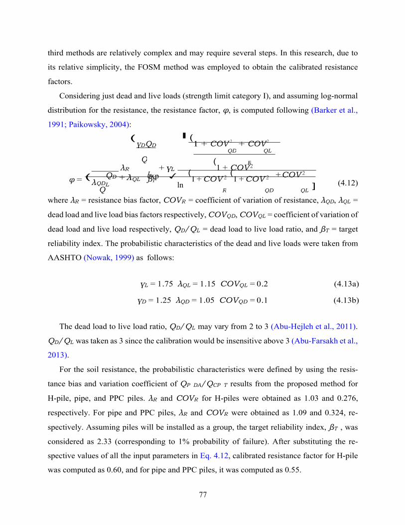
77

R QD QL

(λ

third methods are relatively complex and may require several steps. In this research, due to

its relative simplicity, the FOSM method was employed to obtain the calibrated resistance

factors.

Considering just dead and live loads (strength limit category I), and assuming log-normal

distribution for the resistance, the resistance factor, φ, is computed following (Barker et al.,

1991; Paikowsky, 2004):

(γDQD

I (1 + COV 2 + COV 2

λR + γL L

(1 + COV 2

φ = QD Q

QD QL L

exp βT ✓ ln

(1 + COV 2

(1 + COV 2

+ COV 2

(4.12) ]

where λR = resistance bias factor, COVR = coefficient of variation of resistance, λQD, λQL =

dead load and live load bias factors respectively, COVQD, COVQL = coefficient of variation of

dead load and live load respectively, QD/QL = dead load to live load ratio, and βT = target

reliability index. The probabilistic characteristics of the dead and live loads were taken from

AASHTO (Nowak, 1999) as follows:

γL = 1.75 λQL = 1.15 COVQL = 0.2 (4.13a)

γD = 1.25 λQD = 1.05 COVQD = 0.1 (4.13b)

The dead load to live load ratio, QD/QL may vary from 2 to 3 (Abu-Hejleh et al., 2011).

QD/QL was taken as 3 since the calibration would be insensitive above 3 (Abu-Farsakh et al.,

2013).

For the soil resistance, the probabilistic characteristics were defined by using the resis-

tance bias and variation coefficient of QP DA/QCP T results from the proposed method for

H-pile, pipe, and PPC piles. λR and COVR for H-piles were obtained as 1.03 and 0.276,

respectively. For pipe and PPC piles, λR and COVR were obtained as 1.09 and 0.324, re-

spectively. Assuming piles will be installed as a group, the target reliability index, βT , was

considered as 2.33 (corresponding to 1% probability of failure). After substituting the re-

spective values of all the input parameters in Eq. 4.12, calibrated resistance factor for H-pile

was computed as 0.60, and for pipe and PPC piles, it was computed as 0.55.

Q R

QD QL

+ λ

78

Chapter 5 COMPUTER PROGRAM:

CPILE 5.1 Introduction

CPT-based pile design involves a long computational process. To facilitate the estimation

of pile capacity based on CPT results, a computer program called CPILE was developed.

CPILE has its own user-friendly graphical user interface or GUI. CPILE was developed

using VB.NET programming language, which is an object-oriented programming language

developed by Microsoft beginning 2002. The software is operational on Microsoft Windows

operating system. It follows an easy installation procedure.

5.2 Project Information The first window that appear when CPILE is run is the project information dialogbox.

Figure 5.1 shows the project information window. In this window, information such as

project name, project number, structure number, substructure number, ground elevation,

and ground-water elevation are entered. The project information could be left blank initially

and then updated later.

5.3 Main Window After clicking the Ok button on the project information window, the main window shown in

Figure 5.2 will be loaded. There are eight panels in this window. The first panel, which is

shown in Figure 5.3 is “Input Data Column Locations”. It specifies the input data column

locations corresponding to the depth, cone tip resistance, local sleeve friction, pore pressure,

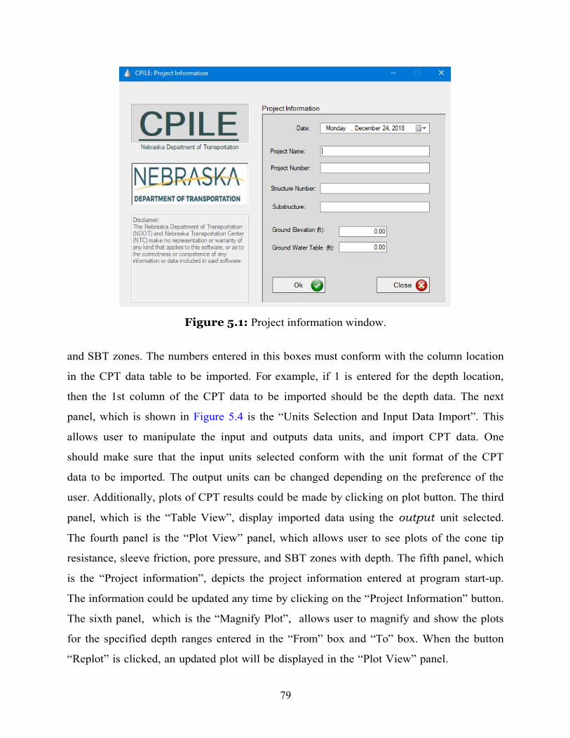
79

Figure 5.1: Project information window.

and SBT zones. The numbers entered in this boxes must conform with the column location

in the CPT data table to be imported. For example, if 1 is entered for the depth location,

then the 1st column of the CPT data to be imported should be the depth data. The next

panel, which is shown in Figure 5.4 is the “Units Selection and Input Data Import”. This

allows user to manipulate the input and outputs data units, and import CPT data. One

should make sure that the input units selected conform with the unit format of the CPT

data to be imported. The output units can be changed depending on the preference of the

user. Additionally, plots of CPT results could be made by clicking on plot button. The third

panel, which is the “Table View”, display imported data using the output unit selected.

The fourth panel is the “Plot View” panel, which allows user to see plots of the cone tip

resistance, sleeve friction, pore pressure, and SBT zones with depth. The fifth panel, which

is the “Project information”, depicts the project information entered at program start-up.

The information could be updated any time by clicking on the “Project Information” button.

The sixth panel, which is the “Magnify Plot”, allows user to magnify and show the plots

for the specified depth ranges entered in the “From” box and “To” box. When the button

“Replot” is clicked, an updated plot will be displayed in the “Plot View” panel.

Figure 5.2: Main window.

80

Figure 5.3: Input data column locations panel.

Figure 5.4: Units selection and data import panel.

The seventh panel is the “Save” panel, which can be used to save the data displayed in

the “Table View” and “Plot View” panels. The table including project information is saved

in *.txt file format while the plots are saved in *.png format. The last panel, which is “Go

To Pile Capacity Analysis”, allows user to select the specific type of CPT-based pile design

desired, that is either H-pile (“H-pile”) or pipe and PPC piles (“P-PPC”).

5.4 H-Pile Window When “H-pile” button, which is found on the “Go To Pile Capacity Analysis” panel within

the main window, is clicked, the “H-pile” window shown in Figure 5.5 will be loaded. In this

window, pile capacity analysis for H-piles is performed. There are six panels in this window.

The first, and the second panels mainly are used to enter the required input parameters such

as pile geometry information and other parameters specifically required for the modified

Tumay and Fakhroo (1982) method. These parameters are summarized in Table 5.1. The

third panel, which is shown in Figure 5.6 is “Pile Capacity Analysis”.

81

Figure 5.5: H-pile window.

82

83

Figure 5.6: Pile capacity analysis panel for H-piles.

In this panel, by clicking the “Compute Pile Capacity” button, pile capacity computation

is performed and computed pile capacity at the specified depth from the ground surface

is displayed. Plots of the variation of toe-capacity, shaft-capacity and total factored pile

capacity can be obtained by clicking on the “Plot Analysis Result” button. The other two

panels are the “Plot View” and “Table” view panels. In these panels, output results are

displayed in plot and tabular format, respectively. Finally, the outputs displayed in the

“Plot View” and “Table View” can be saved by clicking the “Save Data” and “Save Plots”

button found in the “Save” panel.

Table 5.1: Parameters for H-Pile analysis

Input Description Dimensions

Pile width(B) Flange width Unit of length Pile depth(D) Pile cross-sectional depth Unit of length Pile length(L) Pile length Unit of length Influence zone below pile tip (IB)

Influence zone above pile tip (IA)

Influence zone below the pile tip with respect to the pile width, i.e. IB*width(B). Default: IB = 4. Influence zone above the pile tip with respect to the pile width, i.e. IA*width(B). Default: IA = 8.

Dimensionless

Dimensionless

LRFD resistance factor Load resistance factor applied on the nominal pile capacity estimated from CPT results.

Dimensionless

84

5.5 Pipe and PPC piles Window Similar to the H-pile analysis, when the “P-PPC” button found on the “Go To Pile Analysis”

panel in clicked, the “Pipe and PPC piles” window will be displayed, which is shown in

Figure 5.7. There are six panels within this window. The first, and the second panels

mainly are used to enter the required input parameters such as pile geometry information

and other parameters specifically required for the modified De Ruiter and Beringen (1979)

method. These parameters are summarized in Table 5.2. The third panel is the “Pile

Capacity Analysis” panel, which is the same as the one shown in Figure 5.6. In this panel,

by clicking the “Compute Pile Capacity” button, pile capacity computation is performed and

computed pile capacity at the specified depth from the ground surface is displayed. Plots of

the variation of toe-capacity, shaft-capacity and total factored pile capacity can be obtained

by clicking on the “Plot Analysis Result” button. The other two panels are the “Plot View”

and “Table” view panels. In these panels, output results are displayed in plot and tabular

format, respectively. Finally, the outputs displayed in the “Plot View” and “Table View”

can be saved by clicking the “Save Data” and “Save Plots” button found in the “Save” panel.

Figure 5.7: Pipe and PPC pile window.

85

86

Table 5.2: Parameters for Pipe and PPC pile analysis

Input Description Dimensions Pile Diameter (width) (B) Diameter for pipe piles and width for

square PPC piles Pile depth(D) Cross-sectional depth for square PPC

piles. This parameter has no influence on pipe piles

Unit of length

Unit of length

Pile length(L) Pile length Unit of length Influence zone below pile tip (IB) Influence zone below the pile tip with

respect to the pile width, i.e. IB*width(B). Default: IB = 4.

Influence zone above pile tip (IA) Influence zone above the pile tip with respect to the pile width, i.e. IA*width(B). Default: IA = 8.

Cone factor (Nk) A factor that relates the cone tip resistance with undrained shear strength. It is set at a value of 15 by default.

Bearing capacity factor (Nc) A factor that relates the pile unit tip resistance with undrained shear strength. It is set at a value of 9 by default.

Adhesion factor A factor that relates the unit shaft resistance with local sleeve friction from CPT. It is set at a value of 0.5 by default.

LRFD resistance factor Load resistance factor applied on the nominal pile capacity estimated from CPT results.

Dimensionless

Dimensionless

Dimensionless

Dimensionless

Dimensionless

Dimensionless

87

Chapter 6 CONCLUSIONS

This research report looked into the possibility of applying CPT or PCPT-based pile design

methods in the analysis of pile foundations in Nebraska. To get the utmost performances

of the CPT/PCPT-based methods, the calibration of the methods with respect to a more

reliable and accurate pile capacity prediction method is very important. The high strain

dynamic loading test (based on PDA) was sought as a viable option and subsequently used

as a reference pile capacity. Proper adoption of statistical and non-statistical quantitative

evaluation criteria is essential to assess the relative performances in terms of accuracy and

precision of the calibrated CPT/PCPT-based design methods and pick the best performer(s).

After calibration, the modified Tumay and Fakhroo (1982) method showed the best per-

formance for H-piles while the modified De Ruiter and Beringen (1979) method showed the

best performance pipe and PPC piles. The geotechnical uncertainties related to variations

of soil properties, uncertainty in design method predictions, and other construction-related

measurements need to be incorporated in a suitable resistance factor (safety factor) to reach

at a proper design pile capacity. In this case, the LRFD reliability based analysis was con-

ducted to find the appropriate values of resistance factors for each CPT-based design methods

proposed in this study. CPT-based pile design involves a long computational process. To

facilitate the estimation of pile capacity based on CPT results, a computer program called

CPILE was developed. CPILE has its own user friendly graphical user interface (GUI).

88

PART B

CPT-BASED SETTLEMENT

PREDICTION

89

Chapter 1 CPT-BASED SETTLEMENT

PREDICTION

1.1 Introduction

Settlement analysis often plays an important role in the design of bridges, buildings,

plants, etc. For instance, excessive settlement and/or differential movement can cause distor-

tion and crack in the superstructure of bridges. Thus, the potential settlement of foundation

piles must be estimated with great care for such a high-cost structure. The prediction of

pile settlements can be achieved as a sum of the pile settlement and the elastic deformation

of a pile. The soil transitions from the initial stress state (i.e., overburden weight) to a new

one under the additional applied load during the settlement. A major factor that greatly

complicates the foundation design and the settlement prediction is that soil parameters need

to be obtained from the actual construction site. In addition, current methods of the pile

settlement prediction are either too simple (e.g., analytical or semi-analytical) or too com-

plex (e.g., FEM simulation), which adds to the reliability issue of the settlement prediction.

In this research, the team focused on employing the t − z method, which is widely used by FHWA and many state transportation agencies, for the prediction of pile settlement. The

t − z method is a commonly used static analysis for investigating pile load-settlement rela-

tions. This method considers side friction and end bearing at the pile-soil interface as well

as the elastic compression of the pile.

Moreover, the t − z method accounts for different mobilization of side frictions at the

pile-soil interface along the length of the pile, which yields a more reliable estimate given

that the soil behavior is nonlinear and soil profiles are most likely stratified. In this research,

CPT testing data is combined with the t-z method to add confidence in the settlement

prediction.The CPT-based settlement prediction can be categorized as either an analytical

90

approach or numerical approach Figure 1.1.

Figure 1.1: Flowcharts for CPT-based settlement prediction.

1.2 Analytical Approach

The t − z method involves modeling the pile as a series of elements supported by discrete

nonlinear springs, which represent the resistance of the soil in the skin friction (t-z springs),

and a nonlinear spring at the pile tip representing the end-bearing (q −z) spring (Figure 1.2).

The soil springs are nonlinear representations of the soil reaction, t (or q for the pile tip),

versus displacement (z). Assuming the t − z and q − z curves are available, the axial load-

settlement response can be obtained with the aid of a computer program such as TZPILE

and FB-Pier. The site-specific t − z (and q − z) curve may be derived from onsite static load

tests.

In the analytical approach, a given load-transfer t-z function, which defines the relations

between the shaft friction and the relative displacements as well as between the bearing

stress and the pile displacement at the base, is solved to derive a closed-form solution to

predict the pile settlement. During this derivation, CPT test results are used as input data.

The settlement at the top of the pile, ut, can be estimated depending on whether the pile-soil

interface is in the elastic state, elastoplastic state, or plastic state (Misra and Chen,

2004; Haldar and Babu, 2008):

1. elastic state (ξ0 ≥ 1):

ut =

PLp Km

cosh(λ) + ψλ sinh(λ)

λ sinh(λ) + ψλ cosh(λ)

] (1.1)

91

I

t 0 K m 0

K P P λ2ψ

t

2. elastoplastic state (0 ≤ ξ0 ≥ 1):

u = 0.5 (1 − ξ 2

− Lp(q0Lp − p)(

1 − ξ + u

(1.2)

3. plastic state (ξ0 ≤ 0):

u =

PuLp

0.5 + (

P

− 1

+ (

P

− 1 1

(1.3)

where P = applied load at the pile head, Lp = pile length, and q0 = yield strength of the pile-

soil interface that can be obtained as the product of the pile perimeter and the ultimate shear

strength of the pile-soil interface. Axial stiffness of a pile, Km, can be determined from:

Km = EA (1.4) where E = Young’s modulus and A = cross-sectional area of the pile. The scaling factor, λ,

is obtained by: KLp

2 λ =

Km (1.5)

where K = shear modulus of the pile-soil interface.

k1sus K = 2(1 + ν)

(1.6)

where k1 = constant, sus = undrained shear near the pile shaft, and ν = Poisson’s ratio of

the soil. At the pile tip, soil stiffness, Kt,is calculated from:

K = 0.3πDpEt

1 − ν2

(1.7)

where Dp = diameter of pile. Another elastic modulus of soil near the toe, Et, is obtained

from:

Et = k2sub (1.8) where k2 = constant, and sub = average undrained shear strength near the pile tip. Haldar

m

0

t u u

92

(σ

v0

0 λ Q u cosh(λξ0) cosh(λξ0) + ψλ sinh(λ)

and Babu (2008) stated the constants k1and k2 are statistical parameters that follow a log-

normal distribution by analyzing 13 representative pile loading tests. The estimated means

and standard deviations are 1,437 and 437 for k1, and 317 and 144 for k2, respectively. A

non-dimensional factor, ψ, can be determined from:

Kt ψ = KLp

(1.9)

And the interface displacement at yield, u0, can be obtained by:

u = q0

0 K

(1.10)

pu is the ultimate shaft capacity of the pile:

Pu = πDpLpτu (1.11)

where τu = ultimate pile-soil interface shear strength, which can be calculated from:

τs = αsus (1.12)

where α = pile-soil adhesion factor obtained from:

α = 0.5

!

v0

sus

0.45 (1.13)

where σ! = average vertical effective stress over the pile length. Lastly, the value of ξ0 needs

to be calculated by solving the following equations:

(ξ − 1

− tanh(λξ0) + Qt − 1 ψ

(1.14)

In summary, these equations can be embedded into any mathematical software to predict

a potential value of pile settlement with the given inputs. The average undrained shear

strength near the pile shaft, sus, and pile tip, sub, rt above and rb below the pile tip where:

rt =Dp exp (π tan φ) and rb = Dp exp (φ tan φ cos φ), the friction angle of soil φ, and the

93

v0 average vertical effective stress over the pile length σ! are obtained by analyzing CPT data.

1.3 Numerical Approaches In the numerical approach, CPT test results are directly used to derive a proper t-z function

that reflects the shear behavior at the pile-soil interface. There are three widely adopted

models with which the t-z function can be derived: (1) hyperbolic load-transfer curves, (2)

exponential functions, and (3) linear elastic-perfectly-plastic models.

1.3.1 Basic Algorithm

The basic algorithm is briefly described herein: a pile is discretized into N elements (element

length is L0 = Lp/N ) and (N +1) interfaces. The axial load applied on the pile top is Q1 = Qt.

The position of the ith-element is defined by the relative displacement of its upper interface

δi and its lower interface δi+1 (refer Figure 1.2). Axial displacement of a pile depends on the

interaction of the pile with the surrounding soil and its stress state. The shaft resistance Si

is calculated from the unit side friction si and the dimension of the ith-element. The shaft

resistance and axial forces should satisfy force equilibrium.

1.3.2 Load-Displacement (t − z) Functions

Hyperbolic Load-Transfer Curves

Hirayama (1990) suggested the relationships between skin friction f and pile-shaft displace-

ment z, as well as end resistance q and tip displacement ze , based on the Kondner-type

hyperbolic curves: z

f = af + bf z

(1.15)

ze q =

ae + beze

(1.16)

where the constants are bf = 1/fult, be = 1/qult, af = zref,f /fult, and ae = 0.25De/qult (De:

base diameter) in which zref,f is the displacement required to mobilize half of fult (generally

94

(

(a) Overview of pile and t − z function

(b) Numerical simulation algorithm

Figure 1.2: Numerical approach of the CPT-based settlement prediction zref,f ≈ 0.0025Ds; Ds = shaft diameter). Here, fult is the ultimate skin resistance, and qult

is the ultimate tip resistance. Exponential Functions

Gwizdala and Steczniewski (2007) suggested the t − z function for the shaft of pile based on

the power function:

t = qsui z α

for z < zv (1.17) v

where qsui = ultimate soil resistance along the pile within the ith-layer, t = shaft resistance,

z = shaft displacement, and zv = critical shaft displacement, which is defined as 3% of pile

z

95

−

−

diameter. The exponent, α, can be determined using the following formula for a pile that is

installed in cohesive soils:

α = 0.654 0.809 Rsu

Ru

for Rsu

Ru

< 5 (1.18a)

α = 0.25 for Rsu

Ru

> 5 (1.18b)

where Rsu = ultimate soil resistance along the pile shaft and Ru is the ultimate bearing

capacity. For the base of pile, the following power function is used:

( z

β

where qbu = ultimate base resistance, q = base resistance, z = base displacement, and zf =

critical base displacement. The displacement zf of the pile base is assumed as corresponding

to 10% of base diameter: zf = 0.1De. The exponent, β, can be determined using the

following formula:

β = 0.671 0.104 Ru

RB

for Ru

RB < 5 (1.20a)

β = 0.15 for Ru

RB ≥ 5 (1.20b)

where RB = 1.0 MN.

Linear-Elastic-Perfectly-Plastic Model

Pasten and Santamarina (2014) is one of many examples that used a linear-elastic-perfectly-

plastic model as the t − z function to investigate the possible settlement of pile (Figure

1.3).

The side friction Si for the ith-element is defined as: −sult, if

δi + δi+1

≤ −δs

∗

δ + δ

2

i

z f

i − s

q = qbu for z < zf (1.19)

96

i

s

2

i

δ + δ si(δi, δi+1) = ki

i+1 , if δ∗ < i

2 2

δ + δ

i+1

< δs∗

(1.21)

sult, if δ∗ ≤

i+1

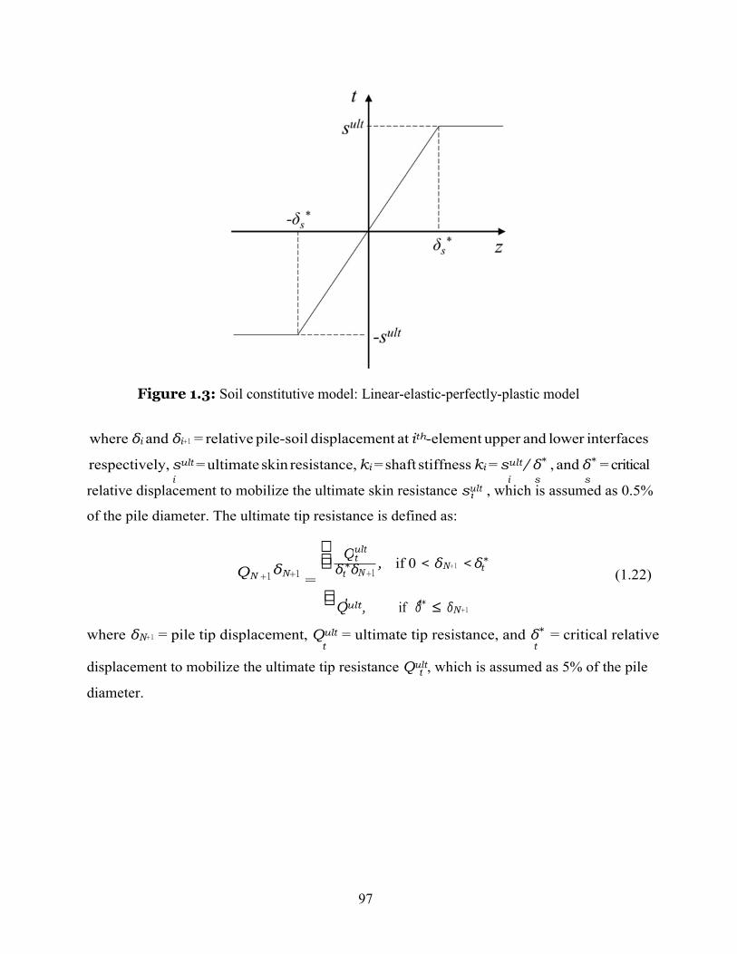
97

i

t

Figure 1.3: Soil constitutive model: Linear-elastic-perfectly-plastic model

where δi and δi+1 = relative pile-soil displacement at ith-element upper and lower interfaces

respectively, sult = ultimate skin resistance, ki = shaft stiffness ki = sult/δ∗ , and δ∗ = critical i i s s

relative displacement to mobilize the ultimate skin resistance sult , which is assumed as 0.5%

of the pile diameter. The ultimate tip resistance is defined as:

QN +1

δN +1 =

ult t

δt∗δN +1

, if 0 < δN+1 < δt∗

(1.22)

Qult, if δ∗ ≤ δN+1

where δN+1 = pile tip displacement, Qult = ultimate tip resistance, and δ∗ = critical relative t t

displacement to mobilize the ultimate tip resistance Qult, which is assumed as 5% of the pile

diameter.

t t

Q

98

1.4 Application 1.4.1 Evaluation Site

We selected SMC1 site for which CPT data is provided by the NDOT. In order to predict

the pile settlement, either through analytical or numerical approaches, ultimate skin and tip

resistances are needed. Soils within the depth of 13.00 m are divided into four layers based

on the CPT data of the evaluation site, using the SBT chart (Robertson et al. (1986); Figure

3.2). The soil layer is shown in Table 1.1. Note that the CPT penetration was conducted

up to the depth of 13.64 m at the evaluation site.

From PART A of this report, it was found that Tumay and Fakhroo (1982) and (De Ruiter

and Beringen, 1979) (European method) are best for calculating the ultimate skin and tip

resistances for the H-pile and the pipe-pile, respectively, with given Nebraska soil conditions.

Details about the the above two CPT-based pile design methods is provided in PART A,

chapter two of this report.

Table 1.1: Soil layers of the evaluation site

5 Clayey silt to silty clay 6 Sandy silt to clayey silt

1.4.2 Pile Types

One type of H-pile and pipe-pile were chosen to evaluate the CPT-based settlement predic-

tion. Properties and dimensions of selected piles are shown in Table 1.2.

Soil layer Depth(m) SBT Zone Soil behavior type 1 0 1.80 7 Silty sand to sandy silt

3 Clay

2 1.80 8.22 4 Silty clay to clay 5 Clayey silt to silty clay

6 Sandy silt to clayey silt

3 8.22 8.34 7 Silty sand to sandy silt 8 Sand to silty sand

3 Clay

4 8.34 13.00 4 Silty clay to clay

99

v0

Table 1.2: Pile type and properties

Pile Type Young’s Modulus (GPa)

Flange width (m)

Diameter (m) Length (m)

H-pile 10x42 200 0.26 0.30 11 Pipe-pile 12.75”

200

-

(equivalent) 0.32

11

1.5 Results 1.5.1 H-Pile

Analytical Approach

For the evaluation site, constants k1 and k2 are chosen as 1,437 and 317, respectively. Other

parameters are as follows: average friction angle of soil within the pile length φ=330 (from

CPT data), pile head force P = 291 kN, Poisson’s ratio ν= 0.35, cross-sectional area of pile

A = 0.0645 m2, diameter of pile Dp = 0.3 m, cross-sectional perimeter of pile S = 1.016 m,

and Young’s modulus of pile E = 200 GPa. The average undrained shear strength near the

pile shaft is sus = 108 kPa, and near the pile tip is Sub = 170 kPa, respectively, based on the

CPT data. The average vertical effective stress over the pile length is σ! =60 kPa. Through

Equation 1.1 to Equation 1.14, pertinent parameters are calculated, and ξ0 is computed as

1.46 ¿ 1. Thus, the pile-soil interface is in the elastic state, and the settlement at the top of

the H-pile is estimated as: ut = 0.53 mm in response to the applied load of 291 kN.

Numerical Approach

Hyperbolic Curve

The pile is divided into 550 elements for the numerical approach. The height of each element

is 0.02 m, which is equal to the cone penetration depth. The ultimate tip resistance qult and

ultimate skin resistance fult of each element are determined by using hyperbolic functions

along with the Tumay and Fakhroo (1982) equation. After that, based on the pile diameter

De, tip resistance qult, and ultimate skin resistance fult, parameters ae, be, af , and bf can be

determined. Then, the force equilibrium is applied to each element with the load-transfer

100

numerical algorithm. Finally, the force on the top of the pile Q1 is calculated. The pile head

force Qhead was preselected as 291 kN. When the calculation error |Q1 − Qhead| ≤ E, where E

is a tolerance value (selected as 5 kN herein), the forward-successive calculation stops. The

distribution of axial forces, skin frictions and displacements of each sub-element along the

pile length are shown in Figure 1.4. The settlement at the top of the pile is estimated as

0.50 mm in response to the applied load of 291 kN.

Figure 1.4: Results of numerical approach to predict the pile settlement using hyperbolic curves for the load-transfer t-z function: H-pile

Exponential Function

Similarly, the ultimate soil resistance, Rsu, ultimate base resistance, qbu, ultimate bearing

capacity Ru, α and β are determined using exponential functions along with the Tumay

and Fakhroo (1982) equation. Based on the equivalent pile diameter De, zv and zf are

determined. The remaining procedures are the same as above, for using a hyperbolic curve

101

for the t − z function. The settlement at the top of the pile is estimated as 0.22 mm. The detailed results are shown in Figure 1.5.

Figure 1.5: Results of numerical approach to predict pile settlement using exponential functions for the load-transfer t − z function: H-pile.

Linear-Elastic-Perfectly-Plastic Model

Again, the ultimate skin resistance, sult, and ultimate tip resistance, Qult, are computed using

i t

the Tumay and Fakhroo (1982) method. Critical displacement thresholds at the pile shaft and

tip, δs∗ and δt

∗, are then determined based on the equivalent pile diameter De. Remaining

procedures are the same as above. The settlement at the top of the pile is estimated as 0.62

mm. The detailed results are shown in Figure 1.6.

102

Figure 1.6: Results of numerical approach to predict pile settlement using linear-elastic- perfectly-plastic models for the load-transfer t − z function: H-pile.

1.5.2 Pipe Pile

Analytical Approach

All the known parameters are the same as with those used for the calculation of H-pile,

except that the applied force at the pile head is changed to P = 214 kN, the cross-sectional

area of a pile is A = 0.0824 m2, the diameter of a pile is Dp = 0.32 m, and the cross-sectional

perimeter of a pile is S = 1.0173 m. Again, pertinent parameters are determined using

Equation 1.1 to Equation 1.14, and the resultant ξ0 is 1.82¿1. Similar to the case of the

H-pile, the pile-soil interface is in the elastic state, and the settlement at the top of the pile

is estimated as ut =0.38 mm in response to the applied load of 214 kN.

103

Numerical Approach

Hyperbolic Curve

The pile-pile is again divided into 550 elements for the numerical analysis. The ultimate

tip resistanceqult and ultimate skin resistance fult of each element are determined using the

De Ruiter and Beringen (1979) method. Other parameters bf , be, af , and ae are calculated

based on the pile diameter De. After that, the force equilibrium is applied to each element

with the load-transfer numerical algorithm. In the end, the force on the top of the pile Q1 is

computed. The pile head force Qhead is 214 kN. When the calculation error |Q1 − Qhead| ≤ E, where E is a tolerance value (selected as 5 kN), the forward-successive calculation stops. The

settlement at the top of the pile is estimated as 0.61 mm in response to the applied load of

214 kN. Detailed results are shown in Figure 1.7.

Figure 1.7: Results of numerical approach to predict pile settlement using hyperbolic curves for the load-transfer t − z function: pipe-pile.

104

Exponential Function Similar to the previous procedures, the ultimate soil resistance, Rsu, ultimate base

resistance, qbu, ultimate bearing capacity Ru, α and β are determined using De Ruiter and

Beringen (1979) (i.e., European Method). And parameters zv and zf are calculated based on

the pile diameter. The remaining procedures are the same as above. The settlement at the

top of the pile is estimated as 0.29 mm. Detailed results are shown in Figure 1.8.

Figure 1.8: Results of numerical approach to predict pile settlement using exponential functions for the load-transfer t − z function: pipe-pile.

Linear-Elastic-Perfectly-Plastic Model

Lastly, the ultimate skin resistance, sult, and ultimate tip resistance, Qult, are obtained using

i t

De Ruiter and Beringen (1979) (i.e., European Method). Critical displacement thresholds

at the pile shaft and tip, δ∗ and δt∗, are then decided based on the pile diameter. Remaining

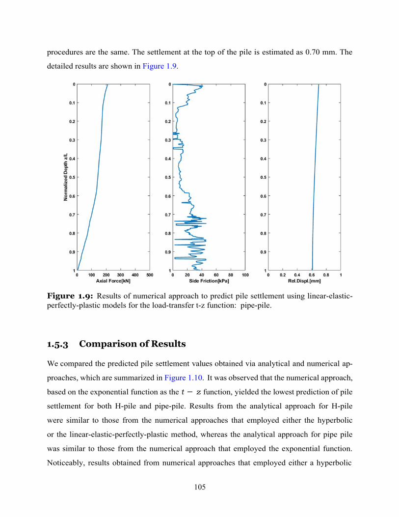
105

procedures are the same. The settlement at the top of the pile is estimated as 0.70 mm. The

detailed results are shown in Figure 1.9.

Figure 1.9: Results of numerical approach to predict pile settlement using linear-elastic- perfectly-plastic models for the load-transfer t-z function: pipe-pile.

1.5.3 Comparison of Results

We compared the predicted pile settlement values obtained via analytical and numerical ap-

proaches, which are summarized in Figure 1.10. It was observed that the numerical approach,

based on the exponential function as the t − z function, yielded the lowest prediction of pile

settlement for both H-pile and pipe-pile. Results from the analytical approach for H-pile

were similar to those from the numerical approaches that employed either the hyperbolic

or the linear-elastic-perfectly-plastic method, whereas the analytical approach for pipe pile

was similar to those from the numerical approach that employed the exponential function.

Noticeably, results obtained from numerical approaches that employed either a hyperbolic

106

curve or a linear-elastic-perfectly-plastic model as the t − z function were almost twice as those of the lowest predictions. Since we only applied these approaches to one investigation

site, applications to more sites in Nebraska and actual field tests would help confirm the

reliability of the suggested CPT-based pile settlement prediction method.

Figure 1.10: Summary of the pile settlement prediction from different approaches.

1.6 Development – Numerical Computation Code MATLAB-based computation code and its graphical user interface (GUI) have been devel-

oped for the prediction of pile settlements that employ different t-z functions of this study.

GUI is convenient for users to import CPT data, and to choose the calculation method and

pile type for the settlement prediction. In order to run the code, input excel file needs to be

prepared by a user. An example of the input excel file is shown in Figure 1.11. The first and

second columns of the input file are the cone tip resistance, qt, and shaft friction, ft, from

the CPT test. The third column of the input file is the zone of soils in the SBT chart. The

fourth column of the input file is the overconsolidation ratio, OCR.

Once the excel-type-of input file is prepared and imported into the GUI (“select file”

button in the GUI; Figure 1.12), settlement prediction can be quickly obtained. Screen shot

of the code GUI is shown in Figure 1.12. First, the pile type needs to be selected between the

107

H-pile and pipe-pile. Then, parameters, such as pile’s diameter, length, Young’s modulus,

and the collection interval of the CPT data need to be filled in (left side of the GUI). Lastly,

a user can select the type of t-z function between the hyperbolic, exponential, and linear-

elastic-perfectly-plastic functions (right side of the GUI). Once the function is hit, the code

will show the settlement prediction (green color in the GUI) as well as the profiles of axial

force, side friction, and relative displacement of the pile along the penetration depth (in

terms of the normalized depth, z/L; Figure 1.12).

Figure 1.11: An example of input excel file to run the code for the settlement prediction of a pile

1.7 Conclusion

CPT-based analytical and numerical computation approaches are proposed and tested for

making a settlement prediction of H-piles and pipe piles in Nebraska. Through the com-

parison of settlement results for these pile types at the investigation site, it was observed

that employing either hyperbolic or linear-elastic-perfectly-plastic models as the t-z function

yields a similar settlement prediction for both pile types. Using an exponential curve as

the t-z function resulted in the lowest settlement prediction among all tested approaches.

108

Figure 1.12: GUI of the code for the settlement prediction of a pile.

Outcomes from the analytical approach lie between those results obtained via the numerical

computation approaches. Since only one investigation site was applied for these approaches,

applications to more sites in Nebraska and actual field tests would help to confirm the relia-

bility of the suggested CPT-based pile settlement prediction method. Finally, a MATLAB-

based computation code that has a graphical user interface (GUI) was developed for the

settlement prediction that will provide a convenient tool for users.

109

Appendices

Table 3: Measured and predicted pile capacities for different methods

SN SS Pile Type CW [kN] EN [kN] M-1 M-2 M-3 M-4 M-5 C05501305P A1 HP12x53 725 552 995.4 366.4 1481 1487.1 1179.7 S034 31644 A1 HP12x53 712 686 606.5 257.26 689.7 1073.6 906 S034 31644 A1 HP12x53 761 782 646 282.35 738.2 1104.2 970.9 S034 31644 A1 HP12x53 818 871 693.8 385 797.9 991.4 1074.3 S034 31644 A2 HP12x53 334 283 696.8 347.7 791.2 930.7 942.1 S034 31644 A2 HP12x53 440 358 798 426.5 905.5 1106.1 1106.8 S034 31644 A2 HP12x53 676 583 821.4 418.13 979.1 1401.1 1201.1 S034 31644 A2 HP12x53 663 577 880.8 516.2 1016.5 1346.8 1298.4 S034 31752 A1 HP12x53 1116 990 843 230.21 871.5 1015.7 844.9 S034 31752 A2 HP12x53 503 483 1770.5 624.6 2481 2078.7 1739.1 S034 31752 B1 HP12x53 1392 1150 1091.8 305.1 1513.4 1553.5 1069.7 S034 31752 B2 HP12x53 1036 765 1761.8 621 2457 2075.6 1735.3 S080 41341 A1 HP12x53 1712 1319 1541.3 571.1 1759.7 1948.7 1247.6 S080 41341 A1 HP12x53 1784 1787 1780.7 688.2 2115.7 2092.3 1632.5 S080 41341 A2 HP12x53 792 1002 1004.3 412.3 1727 1876 1272.9 S159 01373 N3 (P3) HP14x89 1601 1765 1214 542.2 1915.5 2404 1964.6 S159 01373 N2 (P2) HP14x89 2669 2340 1073.3 433.8 2110.3 2421.4 1901.4 C006602905 A2 HP10x42 467 380 995.6 239.8 1024.3 1318.5 916.8 C006602905 A2 HP10x42 512 334 1082.5 261.04 1037.7 1331.4 981.5 C006602905 A2 HP10x42 592 405 1229 315.21 1074.6 1388.6 1170.7 S080 43555 A1 HP12x53 681 394 754.8 599.6 1010.7 1714.1 1174.4 S080 43555 A1 HP12x53 792 560 791.1 639.3 1071.1 1855.7 1264 S080 43555 A1 HP12x53 916 646 891.3 714.5 1224.9 2055.1 1396.7 S080 43555 A1 HP12x53 992 715 1005.8 699.6 1346.8 2437.1 1542 S080 43555 A2 HP12x53 827 766 698.1 615.5 995.4 1592.3 1143.1 S080 43555 A2 HP12x53 912 867 913.6 748.6 1130.5 1843.8 1410.1 S080 43555 A2 HP12x53 1228 953 1137.9 776.2 1330.7 2263.3 1651.5 S080 43555 A2 HP12x53 1379 1013 1130.9 912 1520 2320.8 1758.7 S080 43555 A2 HP12x53 1726 1245 1268 1008.5 1642.5 2555.7 1997.9

109

SN SS Pile Type CW [kN] EN [kN] M-1 M-2 M-3 M-4 M-5 S080 43555 P1 HP12x53 1428 1227 1040.1 802.2 1387.1 2277.7 1613.6 S080 43555 P1 HP12x53 1739 1456 1040.1 802.2 1387.1 2277.7 1613.6 S080 44207 P4 HP12x53 756 785 1427.9 756.31 1747.5 1793.5 1931.6 S080 44207 P4 HP12x53 916 968 1356.8 787.08 1633.8 1623.8 1990.9 S080 44207 P4 HP12x53 1050 1058 1490.5 852.34 1921.7 1843.7 2202.3 S080 44207 P4 HP12x53 1223 1139 1588.3 910.73 2101.7 1960.7 2372.2 S080 44207 P4 HP12x53 1397 1066 1663.9 952.59 2165.9 1975.9 2502 S080 44207 P4 HP12x53 752 727 1336.3 795.7 1655.1 1467.7 1831.4 S080 44207 P4 HP12x53 756 722 1421.1 778.23 1617.1 1633.1 1979.4 S080 44207 P4 HP12x53 956 905 1431.4 821.57 1848.9 1807.9 2106.4 S080 44207 P4 HP12x53 1477 1168 1560.5 897.05 2076.8 1948.8 2332.7 S080 41856 A1 HP12x53 761 542 574.54 502.8 852.62 1074.85 1010.57 S080 41856 A1 HP12x53 712 763 582.17 516.38 874.52 1118.95 1036.51 S080 41856 A1 HP12x53 881 933 662.1 558.58 920.8 1180.51 1120.5 S080 41856 A2 HP12x53 1228 835 1191.2 761.5 1549.9 1623.9 1773.6 S080 41856 A2 HP12x53 1343 1029 1238.8 802.1 1553.7 1665.8 1886.4 S080 41856 A2 HP12x53 1521 1191 1293.7 760.95 1649.4 1923.4 1993.6 S077 09368 A1 pipe 1993 1749 1150.3 618.1 1644.8 2234.9 1644 S077 09368 A2 pipe 1908 1530 1990.2 884.5 2097.7 2854 2241 S077 09368 A2 pipe 2002 1765 2065 930 2219 2924 2488 S077 09368 B1 pipe 2002 1751 1327.3 667.6 2044.6 2610 1937.5 S077 09368 B2 pipe 1913 1698 1873.3 789.3 2009.6 2788 2073.3 S080 08295L A1 pipe 2010 1326 1653.8 657.6 1976.6 1679.2 1859.3 S081 08578 A1 pipe 725 769 598.3 403.03 624.2 1252.23 947.7 S081 08578 A1 pipe 378 644 475.2 327.78 582.6 1145.1 791.24 S081 08578 A1 pipe 436 727 596 356.84 613.7 1303 934.7 S081 08578 A1 pipe 756 821 606.3 369.09 671.3 1360.7 957.1 S081 08578 B2 pipe 609 404 1264.3 890.1 1645.4 1817.4 1708.6 S081 08578 B2 pipe 627 393 1454.1 980.9 1688.7 1828.8 1969.5 S081 08578 B2 pipe 516 440 1389.2 959.2 1755.5 1884.3 1924.9

110

SN SS Pile Type CW [kN] EN [kN] M-1 M-2 M-3 M-4 M-5 S081 08578 B2 pipe 534 445 1317.2 931.5 1794.6 1918.9 1870.6 S080 40436 A1 pipe 854 556 792.01 530.04 962.1 1058.11 1288.31 S080 40436 A1 pipe 729 606 962.8 641.39 1127.4 1291.5 1515.4 S080 40436 A1 pipe 592 640 1078.7 696.16 1361.2 1704.2 1606 S085 0042 P1 pipe 249 316 240.75 223.45 414.5 514.75 405.9 S085 0042 P1 pipe 276 412 262.29 243.28 444.1 567.98 444.41 S085 0042 P1 pipe 316 462 279.65 257.47 474.3 606.94 470.54 S085 0042 P2 pipe 605 739 348.3 298.77 594 808.8 533.58 S085 0042 P2 pipe 614 654 405.7 371.38 714 876.3 652.2 S085 0042 P3 pipe 307 420 351 246.61 893.4 1118.7 665.1 S080 42094 A1 pipe 801 819 937.9 452.59 806.9 895 1284 S080 42094 A1 pipe 734 773 1001.6 479.09 870.4 960.3 1372.2 S080 42094 A1 pipe 676 658 1026.2 505.49 1067 1204.6 1457.9 S080 42094 A1 pipe 983 911 1402.1 773.7 1334.5 1158.3 1904.6 S080 42094 A1 pipe 885 854 1575.9 709.8 1721.6 1654.6 2028.5 S080 42094 A2 pipe 1121 1025 1460.8 630.7 1819.1 2156 1714.2 S080 42094 A2 pipe 1134 980 1575.1 664.8 1285.9 1639 1855.6 S080 42094 A2 pipe 1201 1057 1164.8 593.12 970.3 1329.4 1688.4 S080 42094 A2 pipe 1254 1138 1119.2 602.46 1124.9 1524.4 1703.1 S015 13411 A1 pipe 823 635 534.3 437.43 827.1 1088.9 801.8 S015 13411 A1 pipe 1032 736 592.3 482.9 913.1 1229.7 906.1 S015 13411 A1 pipe 1108 811 650.7 528.7 988.3 1363.4 1007 S015 13411 B1 pipe 876 1066 513.2 421.99 803.5 1048.1 765.5 S015 13411 B1 pipe 907 1325 572.1 467.69 890.7 1186.9 860.9 S015 13411 B1 pipe 992 1092 650.7 528.7 988.3 1363.4 1007 S015 13411 B2 pipe 823 897 994.8 698.5 1321.7 1618.3 1491.3 S015 13411 B2 pipe 894 944 1039.5 735.3 1388.6 1703.3 1581 S015 13411 B2 pipe 965 961 1039.5 735.3 1388.6 1703.3 1581 S080 40436 P1 Type I 738 638 984.5 666.73 1420.2 1339.33 1593.39 S080 42094 P1 Type I 778 765 1196.2 570.8 1215.3 1160.1 1623.4

111

SN SS Pile Type CW [kN] EN [kN] M-1 M-2 M-3 M-4 M-5 S080 42094 P1 Type I 836 917 1081.3 640.1 1110.2 1015.3 1639.4 S080 42094 P1 Type I 863 1104 1598.8 722.2 1666.9 1472.9 2088.6 S080 42094 P1 Type I 707 851 1817.8 818.7 2272.8 1946.8 2314.6 S080 42094 P1 Type I 890 1077 1880.2 884.4 2812 2314 2502.7

Table 4: Measured and predicted pile capacities for different methods

SN SS Pile Type CW [kN] EN [kN] M-6 M-7 M-8 M-9 M-10 M-11 C05501305P A1 HP12x53 725 552 1430.9 929.8 960.4 1141.4 1380.3 908.4 S034 31644 A1 HP12x53 712 686 933.3 467.4 596.6 933.9 1380.3 661 S034 31644 A1 HP12x53 761 782 944.7 526.2 663.3 1019.4 1466.9 872.34 S034 31644 A1 HP12x53 818 871 973.5 581.4 677.3 1109.1 1567.1 1825.5 S034 31644 A2 HP12x53 334 283 880 631.1 656 1012.1 1234.7 2045 S034 31644 A2 HP12x53 440 358 956.2 731.9 729.5 1149.4 1397.3 3860.7 S034 31644 A2 HP12x53 676 583 1007.5 821 700.1 1267 1478.3 5962.87 S034 31644 A2 HP12x53 663 577 1081.2 868.8 745.5 1345.7 1601.8 7286.9 S034 31752 A1 HP12x53 1116 990 1361 487 748.3 733.8 1094.7 257.2 S034 31752 A2 HP12x53 503 483 1777.1 1212.2 1478.3 1499 3056 1397.7 S034 31752 B1 HP12x53 1392 1150 1654.5 788.6 1030.6 1049.5 1540.6 452.4 S034 31752 B2 HP12x53 1036 765 1773.8 1206.4 1473.5 1493.4 3043 1373.7 S080 41341 A1 HP12x53 1712 1319 1858.4 1744.6 1524.4 1756.5 1364.1 1070.2 S080 41341 A1 HP12x53 1784 1787 1912.9 1334.4 1780.1 1317.5 2349 1275.2 S080 41341 A2 HP12x53 792 1002 1911.9 1329.7 1079.8 1413 1151.5 827.1 S159 01373 N3 (P3) HP14x89 1601 1765 2586 1081.3 1323.4 1980.9 2542.1 859.8 S159 01373 N2 (P2) HP14x89 2669 2340 2806 1523.7 1241.3 2086 2289.4 965.7 C006602905 A2 HP10x42 467 380 1073.3 624.31 1020.8 1037 1480.5 339.5 C006602905 A2 HP10x42 512 334 1080.1 659.2 1091.3 1081.9 1549.3 363.6 C006602905 A2 HP10x42 592 405 1104.8 740.2 1248.8 1208.4 1950.3 424.2 S080 43555 A1 HP12x53 681 394 990.8 876 721.4 1099.4 1918 1450.6 S080 43555 A1 HP12x53 792 560 1079.2 931.1 705.8 1156.3 2093.2 1447.7

112

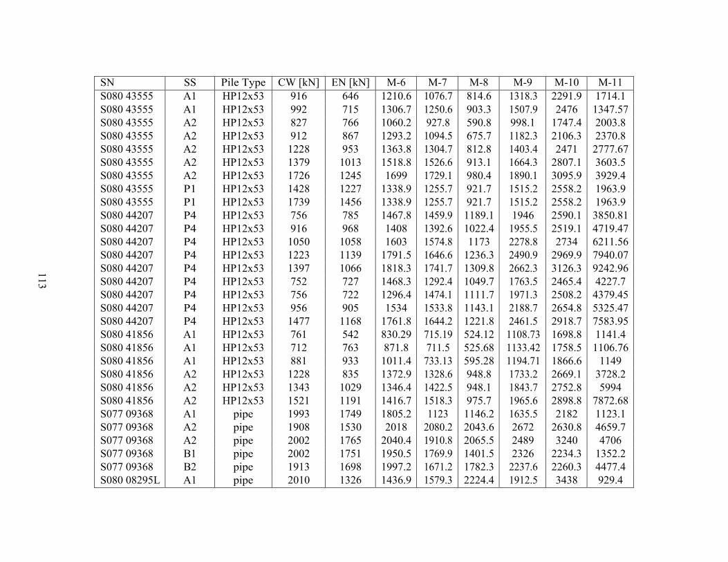
SN SS Pile Type CW [kN] EN [kN] M-6 M-7 M-8 M-9 M-10 M-11 S080 43555 A1 HP12x53 916 646 1210.6 1076.7 814.6 1318.3 2291.9 1714.1 S080 43555 A1 HP12x53 992 715 1306.7 1250.6 903.3 1507.9 2476 1347.57 S080 43555 A2 HP12x53 827 766 1060.2 927.8 590.8 998.1 1747.4 2003.8 S080 43555 A2 HP12x53 912 867 1293.2 1094.5 675.7 1182.3 2106.3 2370.8 S080 43555 A2 HP12x53 1228 953 1363.8 1304.7 812.8 1403.4 2471 2777.67 S080 43555 A2 HP12x53 1379 1013 1518.8 1526.6 913.1 1664.3 2807.1 3603.5 S080 43555 A2 HP12x53 1726 1245 1699 1729.1 980.4 1890.1 3095.9 3929.4 S080 43555 P1 HP12x53 1428 1227 1338.9 1255.7 921.7 1515.2 2558.2 1963.9 S080 43555 P1 HP12x53 1739 1456 1338.9 1255.7 921.7 1515.2 2558.2 1963.9 S080 44207 P4 HP12x53 756 785 1467.8 1459.9 1189.1 1946 2590.1 3850.81 S080 44207 P4 HP12x53 916 968 1408 1392.6 1022.4 1955.5 2519.1 4719.47 S080 44207 P4 HP12x53 1050 1058 1603 1574.8 1173 2278.8 2734 6211.56 S080 44207 P4 HP12x53 1223 1139 1791.5 1646.6 1236.3 2490.9 2969.9 7940.07 S080 44207 P4 HP12x53 1397 1066 1818.3 1741.7 1309.8 2662.3 3126.3 9242.96 S080 44207 P4 HP12x53 752 727 1468.3 1292.4 1049.7 1763.5 2465.4 4227.7 S080 44207 P4 HP12x53 756 722 1296.4 1474.1 1111.7 1971.3 2508.2 4379.45 S080 44207 P4 HP12x53 956 905 1534 1533.8 1143.1 2188.7 2654.8 5325.47 S080 44207 P4 HP12x53 1477 1168 1761.8 1644.2 1221.8 2461.5 2918.7 7583.95 S080 41856 A1 HP12x53 761 542 830.29 715.19 524.12 1108.73 1698.8 1141.4 S080 41856 A1 HP12x53 712 763 871.8 711.5 525.68 1133.42 1758.5 1106.76 S080 41856 A1 HP12x53 881 933 1011.4 733.13 595.28 1194.71 1866.6 1149 S080 41856 A2 HP12x53 1228 835 1372.9 1328.6 948.8 1733.2 2669.1 3728.2 S080 41856 A2 HP12x53 1343 1029 1346.4 1422.5 948.1 1843.7 2752.8 5994 S080 41856 A2 HP12x53 1521 1191 1416.7 1518.3 975.7 1965.6 2898.8 7872.68 S077 09368 A1 pipe 1993 1749 1805.2 1123 1146.2 1635.5 2182 1123.1 S077 09368 A2 pipe 1908 1530 2018 2080.2 2043.6 2672 2630.8 4659.7 S077 09368 A2 pipe 2002 1765 2040.4 1910.8 2065.5 2489 3240 4706 S077 09368 B1 pipe 2002 1751 1950.5 1769.9 1401.5 2326 2234.3 1352.2 S077 09368 B2 pipe 1913 1698 1997.2 1671.2 1782.3 2237.6 2260.3 4477.4 S080 08295L A1 pipe 2010 1326 1436.9 1579.3 2224.4 1912.5 3438 929.4

113

SN SS Pile Type CW [kN] EN [kN] M-6 M-7 M-8 M-9 M-10 M-11 S081 08578 A1 pipe 725 769 924.3 544.1 561 937.8 1446.4 906.7 S081 08578 A1 pipe 378 644 887.2 427.23 467.5 795.23 1293.5 684.6 S081 08578 A1 pipe 436 727 922.8 663 552.3 1060.7 1433.1 618.4 S081 08578 A1 pipe 756 821 993.3 580.6 580 980.3 1501.6 614.49 S081 08578 B2 pipe 609 404 1450.8 1284.6 1041.9 1418.9 2459.3 2046.9 S081 08578 B2 pipe 627 393 1385.7 1474.8 1090.1 1618.1 2607.2 2426.5 S081 08578 B2 pipe 516 440 1422.8 1449.6 998.2 1589.8 2652.9 2403.4 S081 08578 B2 pipe 534 445 1448 1510.1 966.6 1648.9 2684 2610.8 S080 40436 A1 pipe 854 556 997.6 849.61 675.2 1312.85 1525.6 1268.3 S080 40436 A1 pipe 729 606 1170.9 940.55 834.3 1544.26 1833 1477.3 S080 40436 A1 pipe 592 640 1426.2 1102.2 961 1810.4 2147.7 1434.22 S085 0042 P1 pipe 249 316 559.9 264.67 288.31 365.21 774.63 477.35 S085 0042 P1 pipe 276 412 600.4 279.39 302.15 397.01 836.18 477.35 S085 0042 P1 pipe 316 462 634.6 292.95 312.31 421.54 869.92 592.01 S085 0042 P2 pipe 605 739 683.4 496.2 387.3 640 1082.7 552.65 S085 0042 P2 pipe 614 654 777.9 447.29 391.4 580 1195.8 806.3 S085 0042 P3 pipe 307 420 1094.7 578.3 392.5 715.1 929.2 568.98 S080 42094 A1 pipe 801 819 1141.9 799.4 788.1 1298.7 1503.5 840.54 S080 42094 A1 pipe 734 773 937.1 998.3 1067.7 1576.8 1454.8 926.3 S080 42094 A1 pipe 676 658 1307.9 708.6 854.2 1344.89 1654.4 882.5 S080 42094 A1 pipe 983 911 1424.4 865.7 1110.9 1507.96 1904.2 1372.9 S080 42094 A1 pipe 885 854 1558.7 1276 1368.5 1957.8 2471 1395.8 S080 42094 A2 pipe 1121 1025 1988.4 1201.2 1252.5 1603.8 2102 1164.1 S080 42094 A2 pipe 1134 980 1414 1295.4 1438.5 1777.8 2593 1225.3 S080 42094 A2 pipe 1201 1057 1094.6 1023.2 991.2 1610.2 1746.4 1199.62 S080 42094 A2 pipe 1254 1138 1265.9 984.7 1001.1 1649.1 1933.9 1222.54 S015 13411 A1 pipe 823 635 972.9 569.5 513.3 809.3 1397.5 1019.3 S015 13411 A1 pipe 1032 736 1061.5 658.5 550.6 906.5 1600.3 1164.4 S015 13411 A1 pipe 1108 811 1115.4 749.3 606.5 1010.7 1747.4 1315.7 S015 13411 B1 pipe 876 1066 950.5 546.2 504.4 786.8 1342.3 989.4

114

SN SS Pile Type CW [kN] EN [kN] M-6 M-7 M-8 M-9 M-10 M-11 S015 13411 B1 pipe 907 1325 1036.4 629.4 554.7 873 1532.6 1116.3 S015 13411 B1 pipe 992 1092 1115.4 749.3 606.5 1010.7 1747.4 1315.7 S015 13411 B2 pipe 823 897 1283.4 1148.4 852.1 1497.3 2431.1 1893.5 S015 13411 B2 pipe 894 944 1329.3 1234.2 888 1609 2592.8 2014.5 S015 13411 B2 pipe 965 961 1329.3 1234.2 888 1609 2592.8 2014.5 S080 40436 P1 Type I 738 638 1248.4 1021.4 990.96 1640.17 1909.4 1600.3 S080 42094 P1 Type I 778 765 1133.7 1093.4 1453.6 1760.8 1733.4 1073.3 S080 42094 P1 Type I 836 917 1319 773.34 1120.7 1512.26 1674.5 1185.8 S080 42094 P1 Type I 863 1104 1360 1289.3 1726.1 2075.7 2095.1 1365.1 S080 42094 P1 Type I 707 851 1785.3 1802.9 2049.1 2626.5 2809 1693.7 S080 42094 P1 Type I 890 1077 2146 1918.8 2024.2 2829.1 2995 1885.6

Abbreviations SN : Structure Number SS: Substructure CW: CAPWAP EN: LRFD Driving Equation M-1: Aoki and de Alencar (1975) M-2: Clisby et al. (1978) M-3: Schmertmann (1978) M-4: De Ruiter and Beringen (1979) M-5: Philipponnat (1980) M-6: Tumay and Fakhroo (1982) M-7: Prince and Wardle (1982) M-8: Bustamante and Gianeselli (1982) M-9: Almeida et al. (1996) M-10: Eslami and Fellenius (1997) M-11: Takesue et al. (1998)

115

116

References AbdelSalam, S. S., Sritharan, S., and Suleiman, M. T. (2010). “Current design and con-

struction practices of bridge pile foundations with emphasis on implementation of load resistance factor design.” Journal of Bridge Engineering, 15(6), 749–758.

Abu-Farsakh, M. Y., Chen, Q., Haque, N., et al. (2013). “Calibration of resistance factors for drilled shafts for the new fhwa design method..” Report no., Louisiana Transportation Research Center.

Abu-Farsakh, M. Y. and Titi, H. H. (2004). “Assessment of direct cone penetration test methods for predicting the ultimate capacity of friction driven piles.” Journal of Geotech- nical and Geoenvironmental Engineering, 130(9), 935–944.

Abu-Hejleh, N., DiMaggio, J., and Kramer, W. (2011). “Implementation of lrfd geotechnical design for bridge foundations.” Report No. FHWA NHI-10-039, FHWA Resource Center.

Almeida, M. S., Danziger, F. A., and Lunne, T. (1996). “Use of the piezocone test to predict the axial capacity of driven and jacked piles in clay.” Canadian Geotechnical Journal, 33(1), 23–41.

Alvarez, C., Zuckerman, B., and Lemke, J. (2006). “Dynamic pile analysis using capwap and multiple sensors.” GeoCongress 2006: Geotechnical Engineering in the Information Technology Age, 1–5.

Aoki, N. and de Alencar, D. (1975). “An approximate method to estimate the bearing capacity of piles.” Proc., 5th Pan-American Conf. of Soil Mechanics and Foundation En- gineering, Vol. 1, International Society of Soil Mechanics and Geotechnical Engineering Buenos Aires, 367–376.

ASTM-D4945 (2008). “Standard test method for high-strain dynamic testing of deep foun- dations.” D4945.

Axelsson, G. (2002). “A conceptual model of pile set-up for driven piles in non-cohesive soil.” Deep Foundations 2002: An International Perspective on Theory, Design, Construction, and Performance, 64–79.

Bandini, P. and Salgado, R. (1998). “Methods of pile design based on cpt and spt results.” Proceedings of the 1st International Conference on Site Characterization, 967–976.

Barker, R. M., Duncan, J., Rojiani, K., Ooi, P., Tan, C., and Kim, S. (1991). Manuals for the design of bridge foundations: Shallow foundations, driven piles, retaining walls and abut- ments, drilled shafts, estimating tolerable movements, and load factor design specifications and commentary. Number 343.

117

Basu, D., Salgado, R., and Prezzi, M. (2008). “Analysis of laterally loaded piles in multilay- ered soil deposits.

Bloomquist, D., McVay, M. C., and Hu, Z. (2007). “Updating florida department of trans- portation’s (fdot) pile/shaft design procedures based on cpt & dpt data.” Report no., Florida Department of Transportation.

Briaud, J.-L. and Tucker, L. M. (1988). “Measured and predicted axial response of 98 piles.” Journal of Geotechnical Engineering, 114(9), 984–1001.

Buckley, R., Kontoe, S., Jardine, R., Maron, M., Schroeder, F., and Barbosa, P. (2017). “Common pitfalls of pile driving resistance analysis–a case study of the wikinger offshore windfarm.” Offshore Site Investigation Geotechnics 8th International Conference Proceed- ing, Vol. 1246, Society for Underwater Technology, 1246–1253.

Bustamante, M. and Gianeselli, L. (1982). “Pile bearing capacity prediction by means of static penetrometer cpt.” Proceedings of the 2-nd European symposium on penetration testing, 493–500.

Cai, G., Liu, S., Tong, L., and Du, G. (2009). “Assessment of direct cpt and cptu methods for predicting the ultimate bearing capacity of single piles.” Engineering Geology, 104(3-4), 211–222.

Clisby, M., Scholtes, R., Corey, M., Cole, H., Teng, P., and Webb, J. (1978). “An evaluation of pile bearing capacities.” Volume I, Final Report, Mississippi State Highway Department.

Danziger, B., Lopes, F., Costa, A., and Pacheco, M. (1996). “A discussion on the unique- ness of capwap-type analysis.” Proceedings of the Fifth International Conference on the Application of Stress-Wave Theory to Piles, 394–408.

de Jong, G. D. J. (1956). “Wat gebeurt er in de grond tijdens het heien.” De Ingenieur, 68(25), 77–88.

De Ruiter, J. and Beringen, F. (1979). “Pile foundations for large north sea structures.” Marine Georesources & Geotechnology, 3(3), 267–314.

Douglas, B. and Olson, R. (1981). “Soil classification using electronic cone penetrometer.” Symposium on Cone Penetration Testing and Experience, ASCE, New York, 209–227.

Eslami, A., Aflaki, E., and Hosseini, B. (2011). “Evaluating cpt and cptu based pile bearing capacity estimation methods using urmiyeh lake causeway piling records.” Scientia Iranica, 18(5), 1009–1019.

Eslami, A. and Fellenius, B. H. (1997). “Pile capacity by direct cpt and cptu methods applied to 102 case histories.” Canadian Geotechnical Journal, 34(6), 886–904.

Eslami, A. A. and Gholami, A. M. (2006). “Analytical model for the ultimate bearing capacity of foundations from cone resistance.

118

Fellenius, B. H., Brusey, W. G., and Pepe, F. (2000). “Soil set-up, variable concrete modulus, and residual load for tapered instrumented piles in sand.” Performance Confirmation of Constructed Geotechnical Facilities, 98–114.

GRL engineers, I. (2018). “Capwap signal matching software. Accessed: 2018-22-10.

Gwizdala, K. and Steczniewski, M. (2007). “Determination of the bearing capacity of pile foundations based on cpt test results.” Studia Geotechnica et Mechanica, 29(1-2), 55–67.

Haldar, S. and Babu, G. S. (2008). “Reliability measures for pile foundations based on cone penetration test data.” Canadian Geotechnical Journal, 45(12), 1699–1714.

Hannigan, P. J., Goble, G. G., Thendean, G., Likins, G. E., and Rausche, F. (1997). “Design and construction of driven pile foundations-volume i.” Report no.

Hirayama, H. (1990). “Load-settlement analysis for bored piles using hyperbolic transfer functions.” Soils and Foundations, 30(1), 55–64.

Jardine, R. and Bond, A. (1989). “Behaviour of displacement piles in a heavily overconsoli- dated clay.” 12th Int. Conf. Soil Mechanics and Foundation Engineering, 1147–1151.

Komurka, V. E., Wagner, A. B., and Edil, T. B. (2003). “A review of pile set-up.” Proc., 51st Annual Geotechnical Engineering Conference.

Likins, G. and Rausche, F. (2008). “What constitutes a good pda test?.” Proceedings of the Eighth International Conference on the Application of Stress Wave Theory to Piles, 403–407.

Likins, G. E. and Rausche, F. (2004). “Correlation of capwap with static load tests.” Pro- ceedings of the Seventh International Conference on the Application of Stresswave Theory to Piles, Citeseer, 153–165.

Long, J. H. and Wysockey, M. H. (1999). “Accuracy of methods for predicting axial capacity of deep foundations.” Analysis, Design, Construction, and Testing of Deep Foundations, ASCE, 180–195.

Massarsch, K. (2005). “Ground vibrations caused by impact pile driving.” Proc., Envi- ronmental Vibrations: Prediction, Monitoring, Mitigation and Evaluation (ISEV 2005), Taylor & Francis, London, 369–379.

Misra, A. and Chen, C.-H. (2004). “Analytical solution for micropile design under tension and compression.” Geotechnical & Geological Engineering, 22(2), 199–225.

Ng, K. W., Roling, M., AbdelSalam, S. S., Suleiman, M. T., and Sritharan, S. (2012). “Pile setup in cohesive soil. i: experimental investigation.” Journal of Geotechnical and Geoenvironmental Engineering, 139(2), 199–209.

Nguyen, T. D., Lee, J.-H., Kim, S.-R., et al. (2016). “Applicability of cpt-based methods in predicting toe bearing capacities of driven piles in sand.” Acta Geotechnica, 11(2), 359–372.

119

Nowak, A. S. (1999). “Calibration of lrfd bridge design code.” Report no.

Paikowsky, S. G. (2004). Load and Resistance Factor Design (LRFD) for Deep Foundations, Vol. 507. Transportation Research Board.

Pasten, C. and Santamarina, J. C. (2014). “Thermally induced long-term displacement of thermoactive piles.” Journal of Geotechnical and Geoenvironmental Engineering, 140(5), 06014003.

Philipponnat, G. (1980). “Methode pratique de calcul d’un pieu isole, a l’aide du penetrometre statique.” Revue Francaise de Geotechnique, (10), 55–64.

Price, G. and Wardle, I. (1982). “A comparison between cone penetration test results and the performance of small diameter instrumented piles in stiff clay.” Proceedings of the 2nd European Symposium on Penetration Testing, Amsterdam, the Netherlands, Vol. 2, 775–780.

Rausche, F., Alvarez, C., and Likins, G. (2017). “Dynamic loading tests: a state of the art of prevention and detection of deep foundation failures.” 3rd Bolivian International Conference on Deep Foundations, 177–197.

Rausche, F., Goble, G. G., and Likins Jr, G. E. (1985). “Dynamic determination of pile capacity.” Journal of Geotechnical Engineering, 111(3), 367–383.

Rausche, F., Likins, G., Liang, L., and Hussein, M. (2010). “Static and dynamic models for capwap signal matching.” Art of foundation engineering practice, 534–553.

Robertson, P. (1990). “Soil classification using the cone penetration test.” Canadian Geotech- nical Journal, 27(1), 151–158.

Robertson, P. K. and Cabal, K. (2010). “Guide to cone penetration testing for geotechnical engineering.” Gregg Drilling & Testing.

Robertson, P. K., Campanella, R., Gillespie, D., and Greig, J. (1986). “Use of piezometer cone data.” Use of in situ tests in geotechnical engineering, ASCE, 1263–1280.

Schmertmann, J. H. (1978). “Guidelines for cone penetration test: performance and design.” Report no., United States. Federal Highway Administration.

Skov, R. and Denver, H. (1988). “Time-dependence of bearing capacity of piles.” Proc. Third International Conference on the Application of Stress-Wave Theory to Piles. Ottawa, 25– 27.

Smith, E. A. (1962). “Pile-driving analysis by the wave equation.” American Society of Civil Engineers Transactions.

Takesue, K., Sasao, H., and Matsumoto, T. (1998). “Correlation between ultimate pile skin friction and cpt data.” Geotechnical Site Characterization, 2, 1177–1182.

120

Tumay, M. and Fakhroo, M. (1982). “Friction pile capacity prediction in cohesive soils using electric quasi-static penetration tests.” Interim Research Rep, 1.

Wardhana, K. and Hadipriono, F. C. (2003). “Analysis of recent bridge failures in the united states.” Journal of performance of constructed facilities, 17(3), 144–150.